Center for Turbulence ResearchAnnual Research Briefs 2011

49

Wall-modeled large eddy simulation ofshock/turbulent boundary-layer interaction in a

duct

By I. Bermejo-Moreno, J. Larsson, L. Campo, J. Bodart, R. Vicquelin, D.Helmer AND J. Eaton

1. Motivation and objectives

The canonical problem of the interaction of an oblique shock wave impinging uponand reflecting from a turbulent boundary layer (see Fig. 1 for a schematic diagram) hasbeen the focus of extensive research in the fluid dynamics community owing to its rel-evance in aeronautical engineering applications, ranging from efficient inlet design forair-breathing supersonic engines to fluid-structure interaction and noise reduction inhigh-speed aircraft. Experiments (see Dolling 2001; Dupont et al. 2006, 2008; Humbleet al. 2009; Souverein et al. 2010, and references therein) and numerical simulations,both DNS (Wu & Martin 2008; Pirozzoli & Grasso 2006) and LES (Garnier et al. 2002;Touber & Sandham 2009) have greatly increased our understanding of this interactionover the last several decades, but open fundamental questions still remain, such as theorigin of large-scale low-frequency motions (Pirozzoli et al. 2010) and the effects of three-dimensionality in the flow features (Hadjadj et al. 2010), when side walls are present.Numerical simulations are often performed with periodic transverse boundary conditionsthat simplify the simulation by eliminating two side walls but do not allow a characteri-zation of such 3D effects. Recent experiments performed by Helmer & Eaton (2011) weredesigned specifically to address this latter issue.

One of the difficulties that arises when comparing experimental results with numericalsimulations is that the large Reynolds numbers achieved in the experiments are notreproducible in the simulations because of the prohibitive computational cost that wouldbe required to resolve all the scales present in the flow. Direct numerical simulations(DNS) that resolve all scales are therefore limited to relatively low Reynolds numbers. Inlarge-eddy simulations (LES), a compromise is made to reach higher Reynolds numbersby utilizing a sub-grid scale model for the smaller scales of turbulence motion. But eventhen, resolving the boundary layer structures that result from the presence of the wall isstill too expensive for most flow conditions of practical interest. A further step involvesthe use of a wall-model, that greatly reduces the computational cost and allows presentsimulations to reach comparable Reynolds numbers as those found experimentally.

The objective of this study is to perform a wall-modeled large-eddy simulation (WM-LES) of the interaction of an oblique shock and a turbulent boundary layer in a low-aspect-ratio duct that replicates the experimental conditions of Helmer & Eaton (2011),focusing on the effects of three-dimensionality in the flow structure, while evaluating theadequacy of a simple equilibrium wall-model to reproduce the main features observedexperimentally. This would allow further exploration of the flow features that may notbe retrievable through currently available experimental measurement techniques.

This brief is structured as follows. Section 2 describes the flow conditions and the

50 I. Bermejo-Moreno et al.

incident shock

refle

cted

shoc

k

turbulent BL

φ

β

SC

sonic line

relaxation

expansion

fan

com

pre

ssio

nw

aves

shea

rlaye

r

separation bubble

M , Re

Figure 1. Schematic diagram of the shock-turbulent-boundary-layer interaction (adapted fromTouber & Sandham 2009). M and Re are the Mach and Reynolds numbers of the incomingflow, respectively; β is the incident shock angle; φ is the deflection angle experienced by the flowwhen traversing the incident shock; SC is the shock-crossing point, defined as the intersectionbetween the incident and reflected shocks. The presence of a separation bubble is dependent onthe strengths of the adverse pressure gradient resulting from the interaction and the incomingturbulent boundary layer (TBL).

computational setup utilized to replicate the experiment, as well as the description of thenumerical method used to solve the governing equations, with particular emphasis on thewall-model and turbulent inflow. Results of the simulation are presented in section 3 andcompared with those obtained in the experiment, emphasizing the three-dimensionalitythat characterizes this flow. In this regard, the presence of corner flows in the LES ishighlighted. Conclusions and future plans are presented in section 4.

2. Flow conditions and computational setup

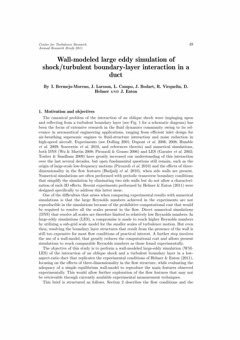
The computational domain (see Fig. 2) consists of a 118 mm-long rectangular constant-area section of 45.2 mm × 47.5 mm, followed by a contraction produced by a 20◦, 3 mm-long wedge that spans the top wall and is responsible for generating the oblique shockthat will impinge and reflect at the bottom wall. Another constant-area section with thenew height resulting from the wedge contraction extends 104 mm farther downstreamafter the wedge.

This domain matches part of the test section of the continuously operated Mach 2.05wind tunnel used in the experiment (see Helmer & Eaton 2011, for details), which fedfrom a 2D converging/diverging nozzle and had a longer development section upstreamof the wedge and also extended farther downstream before exhausting into a plenum. Theturbulent incoming boundary layers had an average thickness of δ0 = 5.4 mm, measured21 mm upstream of the foot of the wedge on the top wall. The Reynolds number based onthe momentum thickness of the incoming boundary layers at that measurement locationwas Reθ ≈ 6, 500. The velocity at the center line was measured to be 525 m/s.

The numerical code named CharLES, developed at the Center for Turbulence Re-search, Stanford University, is employed to perform the numerical simulation of this flow.It is a control-volume-based, finite-volume solver of the spatially filtered, compressibleNavier-Stokes equations on unstructured grids. It uses a third-order Runge-Kutta timediscretization and a grid-based blend of non-dissipative central and dissipative upwindfluxes (see Khalighi et al. 2011, for further details on the numerics). It includes Vreman’ssub-grid scale model (Vreman 2004) and an ENO shock-capturing scheme, active only inregions marked by a shock sensor based on local dilatation and enstrophy (Ducros et al.

Wall-modeled LES of STBLI in a duct 51

x

y

z

wedge

ISW RSW

TBL

TBL

45m

m47

.5mm

43.9

1m

m

118mm 104mm3mm

φw = 20◦

βM = 2.05

Figure 2. Computational setup and main flow features: M, Mach number; TBL, turbulentboundary layers (only top and bottom drawn, for clarity); ISW, incident shock wave; RSW,reflected shock waves; φw, wedge angle; β incident shock angle.

2000). In addition, an equilibrium wall model (Kawai & Larsson 2012) is used, which isdescribed in some detail in subsection 2.1.

The mesh used for this simulation has nearly 30 million control volumes. The gridspacing is uniform in the stream-wise direction, with ∆x = 0.34 mm ≈ δ0/16. In thewall-normal directions (η = y, z), the grid is stretched over a length of 2δ0 from eachwall, with a geometric factor of seven and the grid spacing ranging from ∆η = 0.05 mm≈ δ0/108 at the walls to an isotropic grid (i.e., ∆x = ∆y = ∆z) in the central core. Inviscous units: (∆x+,∆y+,∆z+) ≈ (150, 22 → 150 → 22, 22 → 150 → 22). The resultingnumber of points per direction (x, y, z) is (350+10+308)×(67+70+67)×(74+70+74).

2.1. Wall-modelOwing to the relatively high Reynolds number of the flow under consideration, the gridresolution near the wall is insufficient to resolve all the scales of the boundary layer, andthe use of a wall-model is necessary. In the present simulation, the wall model proposedby Kawai & Larsson (2012) is used. It acts on a refined inner grid which is embedded inthe coarser, outer LES grid (see Fig. 3). In the inner grid, the equilibrium-boundary-layerequations are solved:

ddη

[(µ + µt)

du

dη

]= 0 (2.1)

ddη

[(µ + µt) u

du

dη+ cp

(µ

Pr+

µt

Prt

)dT

dη

]= 0 (2.2)

where η is the wall-normal coordinate, u is the velocity in the stream-wise direction, T isthe temperature, cp is the fluid-specific heat capacity at constant pressure, µ is the fluidmolecular viscosity, Pr is the Prandtl number, Prt is the turbulent Prandtl number andµt is the eddy-viscosity, which is taken from a mixing-length model as

µt = κρηuτ

[1− exp

(− η+

A+

)]2

, A+ = 17, (2.3)

where uτ ≡√

τw/ρ is the friction velocity (characteristic velocity scale in a boundarylayer with varying mean density, based on the wall shear stress, τw) and η+ is the wall-normal coordinate normalized to viscous units, η+ ≡ ρuτη/µ. The model parameters areset constant: κ = 0.41, Prt = 0.9. A matching location is specified (η = 0.05 mm, orin wall units, η+ = 22, in the present simulation), where the exchange of informationbetween both grids/simulations occurs. The inner wall-model simulation takes the LESflow variables (ρ, u, T ) at that location as its free-stream boundary condition (away from

52 I. Bermejo-Moreno et al.

Outer, LES grid

Inner, WM grid

τw, qw

ρ,u, T

matching location

Figure 3. Wall-model schematic diagram.

the wall), whereas the outer LES takes the wall-shear stress and heat-flux at the wall, τw

and qw respectively, from the wall-model inner simulation. The wall-model is applied inall four walls of the LES, considered adiabatic to account for the long period over whichthe batches of PIV image pairs are gathered in the experiment.

2.2. Turbulent inflow

To avoid excessive computational cost, the computational domain comprises only partof the experimental setup. In particular, the domain does not include the converg-ing/diverging nozzle and the initial part of the duct present in the experiment, wherethe boundary layers transition to turbulence. As a consequence, the boundary conditionimposed at the inflow of the simulation must introduce not only mean velocity profilesbut also suitable turbulence quantities that will account for the turbulent nature of theboundary layers, matching those extracted from the experiment. This is achieved by ap-plying the synthetic method of turbulence generation proposed by Xie & Castro (2008),with the modifications of Touber & Sandham (2009), which is based on a digital filteringtechnique (see Klein et al. 2003) designed to match specified single- and two-point cor-relations. In our simulation, the generation of the turbulent inflow boundary conditionis done in several steps:

(a) First, we use the 1D profiles measured in the experiment at a location 21 mmupstream of the foot of the wedge and in four xy-planes (z = 2.5, 4, 5.5 and 21 mm fromone of the side walls) to generate 2D transverse-profiles for the mean and turbulent quan-tities corresponding to that measurement station. This is achieved by using symmetries,interpolation and constant extrapolation from the available experimental data.

(b) Because not all required mean/turbulent quantities are known from the exper-imental data, the 2D reconstructed profiles are used as the inflow to an independentwall-modeled LES of a constant-area duct with a 45.2 mm × 47.5 mm cross section thatmatches the inflow geometry of the final LES. Unknown turbulence quantities are ini-tially set to zero and then let to evolve downstream until the turbulence is fully developedin the boundary layers. At that point, the complete set of 2D profiles for all requiredquantities is extracted from this additional duct-LES, time-averaged after the simulationhas reached a statistically stationary state.

(c) Finally, to provide a boundary layer thickness in the final LES equivalent to theone measured experimentally at the station 21 mm upstream of the foot of the wedge(δ0 = 5.4 mm), the 2D profiles extracted from duct-LES at a downstream location in thecomputational domain are rescaled accordingly. The resulting profiles are then used asthe inflow boundary condition to the LES simulating the experiment.

Wall-modeled LES of STBLI in a duct 53

3. Results

This section presents a comparison of the LES results and the experimental measure-ments. The LES data were time-averaged over approximately 6.5 flow-through times(based on the center-line velocity magnitude), after an initial transient period. In thiscomparison we show first contour plots at four different xy-planes of mean and variancesof the stream-wise and vertical velocity components, emphasizing the 3D effects thatdominate this flow as we move closer to the side walls. Later, we focus on the interactionregion between the incident and reflected shocks and the turbulent boundary layer ofthe bottom wall, by showing 1D mean velocity profiles (stream-wise, x, and vertical, y,components) extracted at several stream-wise locations near the shock-crossing point, inthe z = 21 mm plane, both from the LES and the experiment. The presence of cornerflows found in the LES is highlighted at the end of this section and their stream-wiseevolution is qualitatively described.

3.1. 2D stream-wise/vertical mean and RMS velocity contours

In the experiment, velocity data were acquired through high-resolution, 2D particle imagevelocimetry (PIV) at four xy planes located 2.5 mm, 4 mm, 5.5 mm and 21 mm from oneof the side walls of the tunnel. The first three approximately span the boundary layerof such side wall, while the last plane is located near the center of the tunnel. They arethus targeted at exploring how 3D effects resulting from the presence of the side walls aretranslated into changes of the flow features. Details on the PIV setup and experimentaldata post-processing can be found in Helmer & Eaton (2011).

The same set of data was extracted from the LES and a comparison between exper-imental and simulation results is shown in Figs. 4-7. These figures focus on a regioncomprising both the wedge where the incident shock is generated off the top wall andthe interaction and reflection on the turbulent boundary layer at the bottom wall.

The first observation that can be drawn from Figs. 4 and 5 is that there is a qualitativeagreement between experiment and LES of the flow features in the mean stream-wise andvertical velocities and that the same trends are shown as we move to planes closer tothe side walls. In particular, the shape of the thickened boundary layers near the wedge(x ≈ xwf ≡ wedge foot location) and at the interaction (x − xwf ≈ 45 mm) seen inthe stream-wise velocity (Fig. 4) is well captured by the simulation. Nevertheless, thethickness of the boundary layers appears smaller in the LES than in the experiment. Thisis confirmed when comparing the actual boundary layer thickness at the measurementstation located 21 mm upstream of the foot of the wedge, where the LES shows a δ0 ≈ 5.0mm, almost 10% smaller than in the experiment.

In the experiment it was found that the shock angle resulting from the small 20◦ wedgewas β ≈ 37◦, significantly lower than the 52◦ predicted by inviscid theory. In the LES,an angle of approximately 39◦ is found. A smaller incoming boundary thickness in thesimulation, as previously described, could be responsible for the higher shock angle foundin the LES, when compared with that in the experiment, because viscous effects wouldaffect a smaller region of the flow, bringing the value of that angle slightly closer to theone predicted by inviscid theory.

From the comparison of the vertical velocity contours (Fig. 5) it is observed first thatthe influence of the wedge extends slightly more upstream in the simulation than in theexperiment. At the interaction, the regions found in the experiment in the z = 21 mmplane of high and low negative vertical velocity to the left and right, respectively, of thecrossing point between incident and reflected shocks are also reproduced in the LES,

54 I. Bermejo-Moreno et al.PIV LES

y[m

m]

0

10

20

30

40

x− xwf [mm]−10 0 10 20 30 40 50 60 70 80

y[m

m]

0

10

20

30

40

x− xwf [mm]−10 0 10 20 30 40 50 60 70 80

y[m

m]

0

10

20

30

40

x− xwf [mm]−10 0 10 20 30 40 50 60 70 80

y[m

m]

0

10

20

30

40

x− xwf [mm]−10 0 10 20 30 40 50 60 70 80

y[m

m]

0

10

20

30

40

x− xwf [mm]−10 0 10 20 30 40 50 60 70 80

y[m

m]

0

10

20

30

40

x− xwf [mm]−10 0 10 20 30 40 50 60 70 80

y[m

m]

0

10

20

30

40

x− xwf [mm]−10 0 10 20 30 40 50 60 70 80

y[m

m]

0

10

20

30

40

x− xwf [mm]−10 0 10 20 30 40 50 60 70 80

U [m/s]0 100 200 300 400 500 600

Figure 4. Mean stream-wise velocity contours at span-wise-normal planes located 21, 5.5, 4and 2.5 mm (top to bottom, respectively) from one of the side walls, obtained from PIV (left)and LES (right). Experimental data in white regions on the left plots could not be collected.

although there are some differences in the shape of those regions. Notice that the highershock angle found in the LES brings the shock-crossing point and those high/low-vertical-velocity regions to a location slightly more upstream than in the experiment. Also, thepositive vertical velocity regions found in the experiment immediately downstream of theshock in the vicinity of the wedge for the z = 5.5 and 4 mm planes are also reproducedin the LES, which also shows such a region (although more confined near the wedge) for

Wall-modeled LES of STBLI in a duct 55PIV LES

y[m

m]

0

10

20

30

40

x− xwf [mm]−10 0 10 20 30 40 50 60 70 80

y[m

m]

0

10

20

30

40

x− xwf [mm]−10 0 10 20 30 40 50 60 70 80

y[m

m]

0

10

20

30

40

x− xwf [mm]−10 0 10 20 30 40 50 60 70 80

y[m

m]

0

10

20

30

40

x− xwf [mm]−10 0 10 20 30 40 50 60 70 80

y[m

m]

0

10

20

30

40

x− xwf [mm]−10 0 10 20 30 40 50 60 70 80

y[m

m]

0

10

20

30

40

x− xwf [mm]−10 0 10 20 30 40 50 60 70 80

y[m

m]

0

10

20

30

40

x− xwf [mm]−10 0 10 20 30 40 50 60 70 80

y[m

m]

0

10

20

30

40

x− xwf [mm]−10 0 10 20 30 40 50 60 70 80

V [m/s]−50 −25 0 25 50

Figure 5. Mean vertical velocity contours at span-wise-normal planes located 21, 5.5, 4 and 2.5mm (top to bottom, respectively) from one of the side walls, obtained from PIV (left) and LES(right). Experimental data in white regions on the left plots could not be collected.

the z = 2.5 mm plane, although not observable in the experimental data. The z = 5.5mm plane shows a reflected shock that is somewhat sharper in the LES than in theexperiment, also reaching higher values of the mean vertical velocity.

When examining turbulence quantities (see Figs. 6 and 7) we noted that, whereasa general agreement is observed between experiment and LES, the differences are morenoticeable than in the mean quantities. In particular, the extent near the top and bottom

56 I. Bermejo-Moreno et al.PIV LES

y[m

m]

0

10

20

30

40

x− xwf [mm]−10 0 10 20 30 40 50 60 70 80

y[m

m]

0

10

20

30

40

x− xwf [mm]−10 0 10 20 30 40 50 60 70 80

y[m

m]

0

10

20

30

40

x− xwf [mm]−10 0 10 20 30 40 50 60 70 80

y[m

m]

0

10

20

30

40

x− xwf [mm]−10 0 10 20 30 40 50 60 70 80

y[m

m]

0

10

20

30

40

x− xwf [mm]−10 0 10 20 30 40 50 60 70 80

y[m

m]

0

10

20

30

40

x− xwf [mm]−10 0 10 20 30 40 50 60 70 80

y[m

m]

0

10

20

30

40

x− xwf [mm]−10 0 10 20 30 40 50 60 70 80

y[m

m]

0

10

20

30

40

x− xwf [mm]−10 0 10 20 30 40 50 60 70 80

u′ [m/s]0 25 50 75 100

Figure 6. RMS stream-wise velocity contours at span-wise-normal planes located 21, 5.5, 4 and2.5 mm (top to bottom, respectively) from one of the side walls, obtained from PIV (left) andLES (right). Experimental data in white regions on the left plots could not be collected.

walls where turbulent intensity is significant appears smaller in the simulation than inthe experiment. This is consistent with the previous observation of a thinner boundarylayer thickness upstream of the wedge foot for the LES, but other sources of discrepancyare being investigated (for example, a different shape of the wall-normal profiles of suchRMS quantities resulting from different development of the turbulent boundary layers).Thinner boundary layers would also occur at the side walls and explain the lower values of

Wall-modeled LES of STBLI in a duct 57PIV LES

y[m

m]

0

10

20

30

40

x− xwf [mm]−10 0 10 20 30 40 50 60 70 80

y[m

m]

0

10

20

30

40

x− xwf [mm]−10 0 10 20 30 40 50 60 70 80

y[m

m]

0

10

20

30

40

x− xwf [mm]−10 0 10 20 30 40 50 60 70 80

y[m

m]

0

10

20

30

40

x− xwf [mm]−10 0 10 20 30 40 50 60 70 80

y[m

m]

0

10

20

30

40

x− xwf [mm]−10 0 10 20 30 40 50 60 70 80

y[m

m]

0

10

20

30

40

x− xwf [mm]−10 0 10 20 30 40 50 60 70 80

y[m

m]

0

10

20

30

40

x− xwf [mm]−10 0 10 20 30 40 50 60 70 80

y[m

m]

0

10

20

30

40

x− xwf [mm]−10 0 10 20 30 40 50 60 70 80

v′ [m/s]0 25 50

Figure 7. RMS vertical velocity contours at span-wise-normal planes located 21, 5.5, 4 and 2.5mm (top to bottom, respectively) from one of the side walls, obtained from PIV (left) and LES(right). Experimental data in white regions on the left plots could not be collected.

turbulent intensity found in the simulation for planes near the side wall (z = 2.5, 4 mm),when compared with that of the experiment. The lower values of RMS vertical velocityfound in the simulation for the incident and reflected shock waves may be a consequenceof the dissipative nature of the shock-capturing numerical method in use (consistent withthe theoretical prediction of Larsson 2010).

58 I. Bermejo-Moreno et al.U

/U∞

0.0

0.2

0.4

0.6

0.8

1.0

y/δ00.0 1.0 2.0 3.0

V/U∞

−0.15

−0.10

−0.05

0.00

0.05

y/δ00.0 1.0 2.0 3.0

Figure 8. Mean stream-wise (left) and vertical (right) velocity profiles in the vertical direction,y, extracted from PIV (markers) and LES (lines) on the span-wise normal plane located atz = 21 mm, for several stream-wise locations (-2, 0, 2, 8 mm), relative to the shock-crossingpoint. Wall-normal coordinate is normalized by the boundary layer thickness, δ0, at a location 21mm upstream of the foot of the wedge in the z = 21 mm plane in the experiment and simulation.Lines represent LES results (dashed: x = -2 mm, continuous: x = 0 mm, dashed-dotted: x = 2mm, dotted: x = 8 mm) and markers represent PIV results (up-triangles: x = -2 mm, circles:x = 0 mm, right-triangles: x = 2 mm, squares: x = 8 mm).

3.2. Wall-normal 1D mean velocity profiles at the interaction

We focus our attention now on the interaction region between the incident/reflectedshocks and the turbulent boundary layer at the bottom wall. Fig. 8 shows 1D profilesof the mean stream-wise and vertical velocity components in the z = 21 mm plane, atstream-wise locations x − xSC = −2, 0, 2, 8 mm, where xSC is the shock-crossing point(see Fig. 1). The wall-normal coordinate, y, in those plots has been normalized with theboundary layer thickness found at the measurement station located 21 mm upstream ofthe foot of the wedge, δ0, with corresponding values of 5.4 mm for the experiment and5.0 mm for the LES.

The mean stream-wise velocity profiles extracted from the simulation reflect qualita-tively the shapes and trends observed in the experiment. For example, the fuller profileinside the boundary layer observed for the location 2 mm upstream of the shock-crossingpoint (dashed line) followed by the deceleration at y/δ0 ≈ 1.2 and the subsequent slowincrease in speed away from the wall is well captured in the simulation. Similarly, changesin the slopes of the profiles 2 and 8 mm downstream of the shock-crossing point (dash-dotted and dotted curves, respectively) agree with the experimental results. Nevertheless,quantitatively it is seen that the simulation shows a consistent over-prediction of the ex-perimental values inside the boundary layer (y/δ0 . 1) and an under-prediction outsidethe boundary layer (y/δ0 & 1). These discrepancies might be the result of a different de-velopment of the incoming turbulent boundary layer between experiment and simulationand are presently under investigation.

For the mean vertical velocity, the stream-wise evolution of these profiles is well-captured, showing profile shapes in good agreement with the experiment. The profilesat x = xSC are almost identical. Profiles 2 mm upstream and downstream of the shock-crossing point (dashed and dash-dotted lines, respectively) also show good agreement fory > δ0, whereas inside the boundary layer, the simulation over-predicts the values ob-served in the experiment. Further downstream, the opposite holds: the agreement inside

Wall-modeled LES of STBLI in a duct 59y

[mm

]

0

1

2

3

4

5

6

z [mm]0 1 2 3 4 5 6

z [mm]0 1 2 3 4 5 6

z [mm]0 1 2 3 4 5 6

U [m/s]

100

200

300

400

500

(a) x− xwf = −21 mm (b) x− xwf = 11 mm (b) x− xwf = 28 mm

Figure 9. Downstream evolution (from LES) of corner flow in the vicinity of y = z = 0, forstream-wise locations (relative to the wedge foot): x − xwf =-21, 11 and 28 mm (from left toright). Contours of mean stream-wise velocity, U , are superimposed with arrows representingthe transverse velocity, V ey + Wez, where eα is the versor in the α-coordinate direction.

the boundary layer is good but there is an over-prediction outside. Even then, the shapeof these profiles is remarkably close to the experimental data.

3.3. Corner flowsAn important consequence of the three-dimensionality of the the flow brought in by theside walls in combination with the presence of turbulent boundary layers is the generationof secondary flows of Prandtl’s second kind, referred to in Bradshaw (1987) as “stress-induced secondary flows”, since the gradients of Reynolds stresses produce the stream-wise mean vorticity responsible for such secondary flows. Theoretical, experimental andnumerical studies (Gessner 1973; Gessner et al. 1987; Davis et al. 1986; Joung et al. 2007)have investigated these corner flows occurring in ducts, both in subsonic and supersonicturbulent flow conditions. Nevertheless, the presence of shocks and how they affect theevolution of such corner flows has received less attention and it is targeted in our presentwork. No experimental data were available from Helmer & Eaton (2011) to contrast withthe simulation results, so the following observations are lacking experimental validationand should be taken with care.

Fig. 9 shows contours of mean stream-wise velocity magnitude obtained from the nu-merical simulation in the vicinity of the y = z = 0 corner (bottom left corner, whenlooking downstream) at three different transverse planes upstream of the interaction re-gion, with the transverse velocity vector field superimposed. The first plot correspondsto a location 21 mm upstream of the foot of the wedge, thus unaffected by the incidentshock, and clearly shows that the wall-modeled LES is able to reproduce such cornerflows. Two counter-rotating vortices are noticed at this stream-wise location, which arealmost symmetrical with respect to the y = z line. A moderately strong flow is producedalong this line and directed toward the corner. Note that the vortices are inside theboundary layer (δ0 ≈ 5.0 at this stream-wise location).

As we move downstream (center plot), the downwash generated by the incident shockbreaks the symmetry of the corner flow configuration. Notice in Fig. 5 how the region ofnegative mean vertical velocity that distinguishes the incident shock spreads out near theside wall (bottom plots), compared with the z = 21 mm plane located away from the sidewalls (top plot), for which the incident shock is more sharply defined and has a minimalinfluence on the bottom boundary layer for that streamwise location of x − xwf = 11

60 I. Bermejo-Moreno et al.

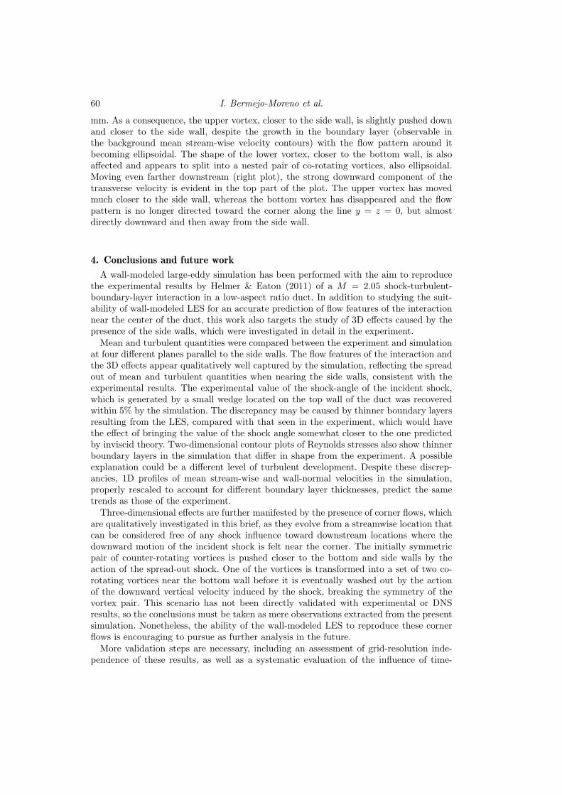
mm. As a consequence, the upper vortex, closer to the side wall, is slightly pushed downand closer to the side wall, despite the growth in the boundary layer (observable inthe background mean stream-wise velocity contours) with the flow pattern around itbecoming ellipsoidal. The shape of the lower vortex, closer to the bottom wall, is alsoaffected and appears to split into a nested pair of co-rotating vortices, also ellipsoidal.Moving even farther downstream (right plot), the strong downward component of thetransverse velocity is evident in the top part of the plot. The upper vortex has movedmuch closer to the side wall, whereas the bottom vortex has disappeared and the flowpattern is no longer directed toward the corner along the line y = z = 0, but almostdirectly downward and then away from the side wall.

4. Conclusions and future work

A wall-modeled large-eddy simulation has been performed with the aim to reproducethe experimental results by Helmer & Eaton (2011) of a M = 2.05 shock-turbulent-boundary-layer interaction in a low-aspect ratio duct. In addition to studying the suit-ability of wall-modeled LES for an accurate prediction of flow features of the interactionnear the center of the duct, this work also targets the study of 3D effects caused by thepresence of the side walls, which were investigated in detail in the experiment.

Mean and turbulent quantities were compared between the experiment and simulationat four different planes parallel to the side walls. The flow features of the interaction andthe 3D effects appear qualitatively well captured by the simulation, reflecting the spreadout of mean and turbulent quantities when nearing the side walls, consistent with theexperimental results. The experimental value of the shock-angle of the incident shock,which is generated by a small wedge located on the top wall of the duct was recoveredwithin 5% by the simulation. The discrepancy may be caused by thinner boundary layersresulting from the LES, compared with that seen in the experiment, which would havethe effect of bringing the value of the shock angle somewhat closer to the one predictedby inviscid theory. Two-dimensional contour plots of Reynolds stresses also show thinnerboundary layers in the simulation that differ in shape from the experiment. A possibleexplanation could be a different level of turbulent development. Despite these discrep-ancies, 1D profiles of mean stream-wise and wall-normal velocities in the simulation,properly rescaled to account for different boundary layer thicknesses, predict the sametrends as those of the experiment.

Three-dimensional effects are further manifested by the presence of corner flows, whichare qualitatively investigated in this brief, as they evolve from a streamwise location thatcan be considered free of any shock influence toward downstream locations where thedownward motion of the incident shock is felt near the corner. The initially symmetricpair of counter-rotating vortices is pushed closer to the bottom and side walls by theaction of the spread-out shock. One of the vortices is transformed into a set of two co-rotating vortices near the bottom wall before it is eventually washed out by the actionof the downward vertical velocity induced by the shock, breaking the symmetry of thevortex pair. This scenario has not been directly validated with experimental or DNSresults, so the conclusions must be taken as mere observations extracted from the presentsimulation. Nonetheless, the ability of the wall-modeled LES to reproduce these cornerflows is encouraging to pursue as further analysis in the future.

More validation steps are necessary, including an assessment of grid-resolution inde-pendence of these results, as well as a systematic evaluation of the influence of time-

Wall-modeled LES of STBLI in a duct 61

averaging period used to collect statistics. The effect of different matching locations uti-lized in the wall-model should also be studied, focusing particularly on how shock-free,shock-interaction and corner regions might be affected by such a parameter. Ensuringa better match with the experiment for the incoming boundary layers (both thicknessand turbulent development) is currently being addressed. Finally, new simulations areplanned with a modified geometry that includes a 3 mm-high wedge to study the case ofshock-turbulent-boundary-layer interaction with flow separation.

Acknowledgments

Financial support has been provided by the United States Department of Energy un-der the Predictive Science Academic Alliance Program (PSAAP) at Stanford University.The authors are grateful to Dr. Joseph W. Nichols for his valuable comments and re-marks on a preliminary version of this manuscript. The authors acknowledge the followingaward for providing computing resources that have contributed to the research resultsreported in this brief: “MRI-R2: Acquisition of a Hybrid CPU/GPU and VisualizationCluster for Multidisciplinary Studies in Transport Physics with Uncertainty Quantifica-tion” http://www.nsf.gov/awardsearch/showAward.do?AwardNumber=0960306. Thisaward is funded under the American Recovery and Reinvestment Act of 2009 (PublicLaw 111-5).

REFERENCES

Bradshaw, P. 1987 Turbulent secondary flows. Annu. Rev. Fluid Mech. 19, 53–74.Davis, D. O., Gessner, F. B. & Kerlick, G. D. 1986 Experimental and numerical

investigation of supersonic turbulent flow through a square duct. AIAA J. 24 (1508).Dolling, D. S. 2001 Fifty years of shock-wave/boundary-layer interaction research:

what next? AIAA J. 39, 1517.Ducros, F., Laporte, F., Souleres, T. & Guinot, V. 2000 High-order fluxes for

conservative skew-symmetric-like schemes in structures meshes: Application to com-pressible flows. J. Comput. Phys. 161, 114.

Dupont, P., Haddad, C. & Debieve, J. 2006 Space and time organization in a shock-induced separated boundary layer. J. Fluid. Mech 559, 255–277.

Dupont, P., Piponniau, S., Sidorenko, A. & Debive, J. 2008 Investigation byparticle image velocimetry measurements of oblique shock reflection with separation.AIAA J. 48 (6), 1365–1370.

Garnier, E., Sagaut, P. & Deville, M. 2002 Large eddy simulation ofshock/boundary-layer interaction. AIAA J. 40 (10).

Gessner, F. B. 1973 The origin of secondary flow in turbulent flow along a corner. J.Fluid Mech. 58, 1–25.

Gessner, F. B., Ferguson, S. D. & Lo, C. H. 1987 Experiments on supersonicturbulent flow development in a square duct. AIAA J. 25 (690).

Hadjadj, A., Larsson, J., Morgan, B. E., Nichols, J. W. & Lele, S. K. 2010Large-eddy simulation of shock/boundary-layer interaction. Annu. Res. Briefs pp.141–152.

Helmer, D. & Eaton, J. 2011 Measurements of a three-dimensional shock-boundarylayer interaction. Tech. Rep. TF-126. Flow Physics and Computational EngineeringGroup, Department of Mechanical Engineering, Stanford University.

62 I. Bermejo-Moreno et al.

Humble, R., Elsinga, G., Scarano, F. & van Oudheusden, B. 2009 Three-dimensional instantaneous structure of a shock wave/turbulent boundary layer in-teraction. J. of Fluid Mech. 622, 33–62.

Joung, Y., Choi, S. U. & Choi, J.-I. 2007 Direct numerical simulation of turbulentflow in a square duct: Analysis of secondary flows. J. Eng. Mech. 213, 213–221.

Kawai, S. & Larsson, J. 2012 Wall-modeling in large eddy simulation: length scales,grid resolution and accuracy. Phys. Fluids (to appear).

Khalighi, Y., Nichols, J. W., Lele, S., Ham, F. & Moin, P. 2011 Unstructuredlarge eddy simulations for prediction of noise issued from turbulent jets in variousconfigurations. AIAA 2886.

Klein, M., Sadiki, A. & Janicka, J. 2003 A digital filter based generation of inflowdata for spatially developing direct numerical or large eddy simulations. J. Comput.Phys. 186, 652–665.

Larsson, J. 2010 Effect of shock-capturing errors on turbulence statistics. AIAA J.48 (7), 1554–1557.

Pirozzoli, S. & Grasso, F. 2006 Direct numerical simulation of impinging shockwave/turbulent boundary layer interaction at m = 2.25. J. Comput. Phys. 18 (6),065113–1–17.

Pirozzoli, S., Larsson, J., Nichols, J. W., Bernardini, M., Morgan, B. E. &Lele, S. K. 2010 Analysis of unsteady effects in shock/boundary layer interactions.Annu. Res. Briefs pp. 153–164.

Souverein, L., Dupont, P., Debieve, J., van Dussaugen, J., Oudheusden, B.& Scarano, F. 2010 Effect of interaction strength on unsteadiness in turbulentshock-wave-induced separations. AIAA J. 48, 1480–1493.

Touber, E. & Sandham, N. 2009 Large-eddy simulation of low-frequency unsteadinessin a turbulent shock-induced separation bubble. Theor. Comput. Fluid Dyn. 23, 79–107.

Vreman, A. W. 2004 An eddy-viscosity subgrid-scale model for turbulent shear flow:Algebraic theory and applications. Phys. Fluids 16 (10), 3670–3681.

Wu, M. & Martin, M. 2008 Analysis of shockmotion in shockwave and turbulentboundary layer interaction using direct numerical simulation data. J. Fluid Mech.594, 71–83.

Xie, Z.-T. & Castro, I. P. 2008 Efficient generation of inflow conditions for large eddysimulation of street-scale flows. Flow Turbul. Combust. 81 (3), 449–470.