Cellular Automata Complexity Threshold and Classification

Cellular Automata Complexity Threshold and Classification: A Geometric Perspective

Mohamed Al-EmamCairo UniversityFaculty of Engineering, Electronics, and Communications DepartmentGiza, Cairo, [email protected]

Vitaliy KaurovWolfram Research, Inc.100 Trade Center DriveChampaign, IL 61820

This paper presents the results of mathematical experiments on the so-called !orientation vector." It looks at complexity in terms of three per-spectives: Wolfram, Langton, and Chua. Critically, we consider Chua#sgeometrical complexity index and a complexity-based classification ofelementary cellular automata. Ideas in terms of solutions for ordinarydifferential equations and complexity measurements are proposed tothe research community for discussion.

Introduction1.

During the Wolfram Science Summer School 2012, I worked on theproject !Investigation of the Relation between Nonlinear DynamicalSystems and Elementary Cellular Automata." The project dealt withChua#s [1] geometrical representation of elementary cellular automata(ECAs) and led to these thoughts about the complexity threshold andmeasurement comparisons.

From an application point of view, Wolfram [2] shows a huge di-versity for mathematical modeling of snowflakes, vegetation,seashells, and other natural forms in terms of ECAs. These mathemati-cal models are explicitly considered as discrete dynamical systems andinformation-processing systems. Dynamical systems analysis in phasespace (state space) proposes the following three behaviors [3].

$ Homogeneous dynamics (fixed point). These tend to stabilize as a sin-gle point in the phase space that is fixed over time. The initial condi-tions significantly determine the long-term behavior; similar initial con-ditions give the same phase plane trajectories.

Complex Systems, 23 % 2014 Complex Systems Publications, Inc.

$ Periodic (limit cycle). These tend to stabilize as a closed path in thephase space. The initial conditions significantly determine the long-termbehavior; similar initial conditions give the same phase planetrajectories.

$ Aperiodic (chaotic, strange attractors). These never seem to stabilize;however, the subspace in which the state path trajectory moves is re-stricted to a bounded manifold. This manifold often possesses complex,detailed structure. In general, similar initial states do not produce sim-ilar state path trajectories, making them insensitive to initialconditions [4].

One of the main questions about ECAs is if they can be used asmathematical models for ordinary differential equations (ODEs).There is more than one answer to that question. We compare the pro-posed criterion inspired by Chua#s cubical representations for ECAs[1] and the other two criteria.

Wolfram!s Classification2.

Wolfram#s classification scheme [2] is phenomenological; that is, theECA space is separated into four classes by visually inspecting space-time diagrams to evaluate their qualitative behavior and complexity(Figure 1):

$ Class I. Steady state, representing homogeneous dynamics.

$ Class II. Repetitive cycles, representing periodic dynamics.

$ Class III. Random-like behavior, representing chaotic patterns.

$ Class IV. Complex behavior, representing complex patterns with localstructures that move through space and time.

Wolfram conjectures that class IV cellular automata (CAs) are com-putationally universal.

Figure 1. Wolfram#s classification for ECAs.

356 M. Al-Emam and V. Kaurov


Langton's " Parameter 3.

In 1990, Langton [5] discussed the question, under what conditionswill physical systems support the basic operations of informationtransmission, storage, and modification constituting the capacity tosupport computation? His answer was, systems near a continuous(second-order) phase transition. These systems that are near critical-ity, between an ordered (!solid") and chaotic (!liquid") state, are espe-cially capable of computations. In other words, ECA rules represent(some part of) the physical world. The initial configuration itself con-stitutes the computer, the program, and the data. Langton translatesthe original question into, when is it possible to adopt this view to un-derstand ECA dynamics?

Lambda values range between 0 and 1 and are calculated as thefraction of ECA rules that lead to a new state with a live cell, ex-pressed as a decimal. This means that the more ECA rules that lead tolife, the larger the & value. An ECA space starting from & ' 0 is fixed(ordered, cold, and predictable). By increasing &, the system changesfrom ordered to what is called periodic (predictable but recurring),then it changes to complex (where the best life simulations comeabout), and finally, above this, the systems are chaotic (messy, unpre-dictable, and hot).

Wolfram#s classification and Langton#s & parameter (Figure 2) cor-respond as follows. CAs with very low & values are very likely to beclass I. CAs with very high & values are very likely to be class III. As &increases, we expect a transition from class I to class II to class IV toclass III. But sharp transitions are not always obtained, and some-times we might go backward. Furthermore, class IV CAs are rare.

Figure 2. Langton#s & parameters for ECA.

Chua!s Complexity Index #4.

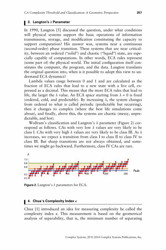
Chua [1] introduced an idea for measuring complexity he called thecomplexity index (. This measurement is based on the geometricalanalysis of separability, that is, the minimum number of separating

CA Complexity Threshold and Classification: A Geometric Perspective 357


y p y p gplanes. We have six real variables )z2, z1, z0; b1, b2, b3* and two inte-gers +1. By making substitutions, configurations are generated forthose variables assigned to the ECA space (Figure 3). We make somestatistical studies on those outputs, finding more acceptable configura-tions for )z2, z1, z0; b1, b2, b3* and two integers +1, that is, the mini-mum number of (. This leads to the complexity index of a local rule,which characterizes the geometrical structure of the correspondingBoolean cube, namely, the minimum number of parallel planes neces-sary to separate the colored vertices. Hence, all linearly separablerules have a complexity index of ( ' 1.

Figure 3. Rule 30 represented geometrically.

Vertex Projection on an Orientation Vector and Number of Transitions

4.1

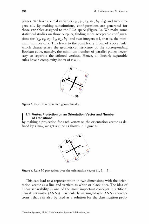
By making a projection for each vertex on the orientation vector as de-fined by Chua, we get a cube as shown in Figure 4.

Figure 4. Rule 30 projection over the orientation vector )1, 3, ,3*.

This can lead to a representation in two dimensions with the orien-tation vector as a line and vertices as white or black dots. The idea oflinear separability is one of the most important concepts in artificialneural networks (ANNs). Particularly in single-layer ANNs (percep-trons), that can also be used as a solution for the classification prob-



p

lem in machine learning. Chua [1] introduces a way to express anODE as an ECA and then make use of that in ANN applications.

The notion of linear separability assumes that there is a pattern set-. This set is divided into subsets -1, -2, . , -R, respectively. If alinear machine can classify the patterns from -i as belonging to classi, for i ' 1, 2, . , R, then the pattern sets are linearly separable.Using this property of the linear discriminant functions, the notion oflinear separability can be stated more formally. If R linear functionsof x exist such that:

gi/x0 1 gj/x0 for all x 2 Xi, i ' 1, 2, . , R;

j ' 1, 2, . , R, i 3 j,

then the pattern sets Xi are linearly separable.Geometrically, linear separability can be extended in n dimensions

to be the hyperplane separating the two sets of points. By countingthe alternations of vertex colors on the vector, that is, using the two-dimensional line to check for color alternations, we can indicatewhether a CA is linearly separable or not.

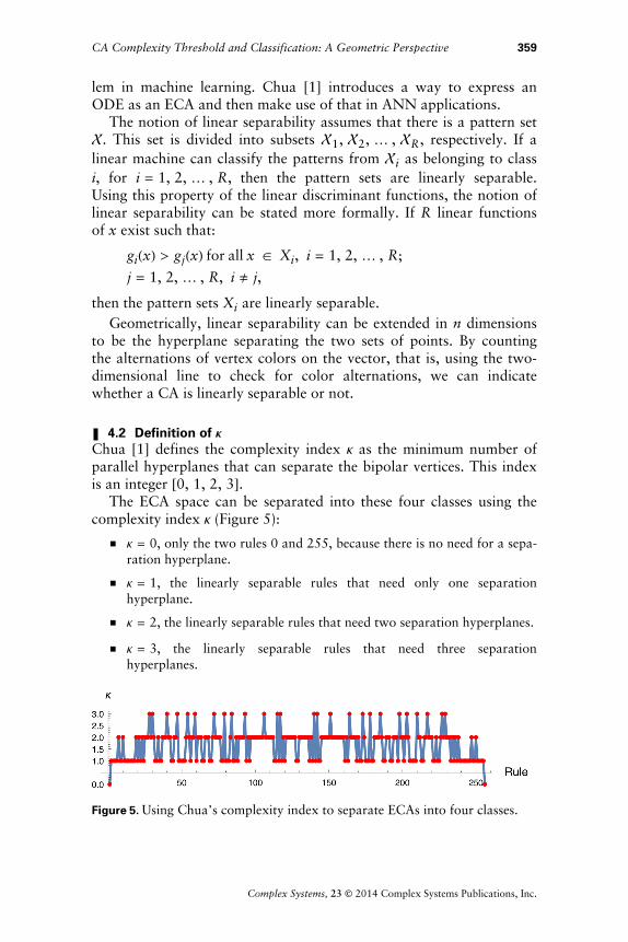
Definition of #4.2Chua [1] defines the complexity index ( as the minimum number ofparallel hyperplanes that can separate the bipolar vertices. This indexis an integer 40, 1, 2, 35.

The ECA space can be separated into these four classes using thecomplexity index ( (Figure 5):

$ ( ' 0, only the two rules 0 and 255, because there is no need for a sepa-ration hyperplane.

$ ( ' 1, the linearly separable rules that need only one separationhyperplane.

$ ( ' 2, the linearly separable rules that need two separation hyperplanes.

$ ( ' 3, the linearly separable rules that need three separationhyperplanes.

Figure 5. Using Chua#s complexity index to separate ECAs into four classes.



Parameters that Influence ! 4.3We found that ! is influenced by some parameters in the equivalentODE of an ECA. Focusing only on the influence of the orientationvector, we found some odd values for !, such as ! " 4. In otherwords, varying the orientation vector led to variations in !. We alsofound that ! is sensitive to that variation.

Part of the study was stepping from #$4, 4% with various step val-ues to generate ODE parameters and then check the correspondingECA. Additionally, the number of transitions is calculated, to indicatethe linear separability; its minimum number represents the value of !.Figure 6 shows the rules versus the number of transitions. Those tran-sitions need to be refined; that is, we need to calculate the minimumnumbers that converge to be candidate ! values.

&a' &b'

&c'

Figure 6. Configurations versus number of transitions ! for (a) secondstep " 2, (b) second step " 1, and (c) third step " 0.6.

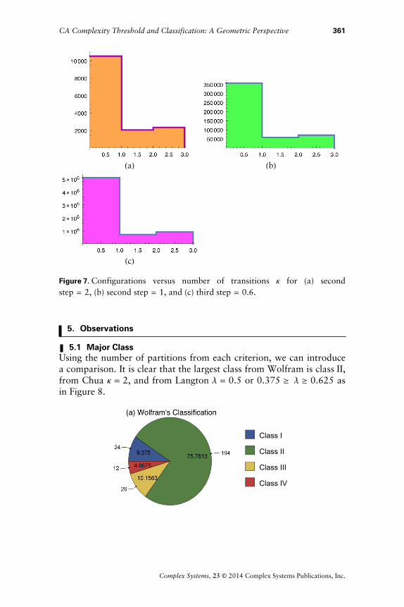
We started by eliminating the ! " 4 configuration values and thentaking the minimum values of ! in each step. We were surprised tofind typical results (Figure 7). That means we got a true ! and a largenumber of values for the orientation vector.


Complex Systems, 23 ( 2014 Complex Systems Publications, Inc.

/a0 /b0

/c0

Figure 7. Configurations versus number of transitions ( for (a) secondstep ' 2, (b) second step ' 1, and (c) third step ' 0.6.

Observations 5.

Major Class5.1Using the number of partitions from each criterion, we can introducea comparison. It is clear that the largest class from Wolfram is class II,from Chua ( ' 2, and from Langton & ' 0.5 or 0.375 6 & 6 0.625 asin Figure 8.

Class I

Class II

Class III

Class IV



!"0

!"1

!"2

!"3

#"0

#"0.125

#"0.25

#"0.375

#"0.5

#"0.625

#"0.75

#"0.875

#"1

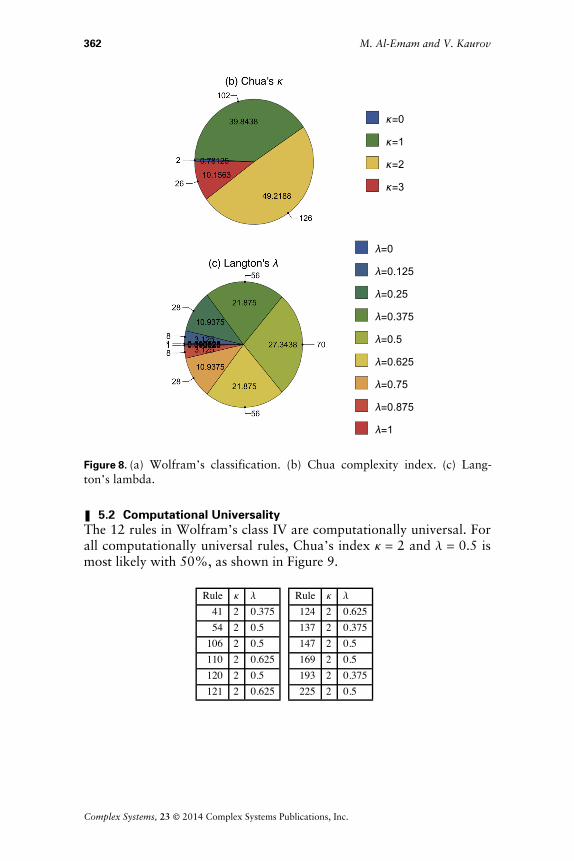
Figure 8. (a) Wolfram#s classification. (b) Chua complexity index. (c) Lang-ton#s lambda.

Computational Universality5.2The 12 rules in Wolfram#s class IV are computationally universal. Forall computationally universal rules, Chua#s index ( ' 2 and & ' 0.5 ismost likely with 50%, as shown in Figure 9.

Rule ( &41 2 0.37554 2 0.5

106 2 0.5110 2 0.625120 2 0.5121 2 0.625

Rule ( &124 2 0.625137 2 0.375147 2 0.5169 2 0.5193 2 0.375225 2 0.5



!"1

!"2

!"3

#"0.375

#"0.5

#"0.625

Figure 9. (a) Chua#s complexity index ( for universal computation. (b) Lang-ton#s & for computationally universal ECAs.

Linear Separability5.3Linear separability is a vital concept in terms of Chua#s definition ofcomplexity because it is this set of rules that needs only one line/planeto separate the bicolor projected orientation vector. There are 102 lin-early separable rules with a Chua complexity index of ( ' 1. Linearseparability is distributed over the & space with a symmetrical distribu-tion as shown in Figure 10. Wolfram#s class II gives the largest set oflinearly separable rules with about 82%; it is clear that both class-es III and IV are missing from Figure 10.

Rule Class &

1 1 0.1252 2 0.1253 2 0.254 2 0.1255 2 0.257 2 0.3758 2 0.125

10 2 0.2511 2 0.375

Rule Class &

12 2 0.2513 2 0.37514 2 0.37515 2 0.516 2 0.12517 2 0.2519 3 0.37521 2 0.37523 3 0.5

Rule Class &

31 3 0.62532 2 0.12534 2 0.2535 2 0.37542 4 0.37543 2 0.547 2 0.62548 2 0.2549 2 0.375



Rule Class &

50 2 0.37551 2 0.555 4 0.62559 2 0.62563 2 0.7564 2 0.12568 2 0.2569 2 0.37576 3 0.37577 2 0.579 2 0.62580 2 0.2581 2 0.37584 2 0.37585 2 0.587 3 0.62593 2 0.62595 2 0.75

112 2 0.375113 2 0.5115 2 0.625117 2 0.625119 2 0.75127 3 0.875128 2 0.125

Rule Class &

136 3 0.25138 4 0.375140 2 0.375142 2 0.5143 2 0.625160 2 0.25162 3 0.375168 2 0.375170 4 0.5171 2 0.625174 2 0.625175 2 0.75176 2 0.375178 2 0.5179 2 0.625186 2 0.625187 2 0.75191 2 0.875192 2 0.25196 3 0.375200 2 0.375204 2 0.5205 2 0.625206 2 0.625207 2 0.75

Rule Class &

208 2 0.375212 2 0.5213 2 0.625220 2 0.625221 2 0.75223 2 0.875224 2 0.375232 2 0.5234 2 0.625236 1 0.625238 2 0.75239 1 0.875240 1 0.5241 2 0.625242 2 0.625243 2 0.75244 2 0.625245 2 0.75247 2 0.875248 2 0.625250 1 0.75251 1 0.875252 1 0.75253 1 0.875254 1 0.875

#"0.125

#"0.25

#"0.375

#"0.5

#"0.625

#"0.75

#"0.875



Class I

Class II

Figure 10. (a) Langton#s & for linearly separable ECAs. (b) Wolfram#s classifica-tion for linearly separable ECAs.

Complexity Threshold5.4The complexity threshold is related to the chosen system and willvary over the three systems in this paper. For our purposes, the ECAis the system; that is, Wolfram#s point of view is computation, Lang-ton#s point of view is information, and Chua#s point of view is ODEor dynamical systems. The complexity threshold from Wolfram isclass III, from Langton it is the area of &, and from Chua it is ( ' 2.

Rules 0 and 255 5.5Rules 0 and 255 were the most commonly found configurations in theexperiment of stepping the orientation vector. Notice that the numberof configurations for these rules is not affected before/after the filtra-tion because no separating planes are needed. Also observe the largepercentage of rule 255 configurations (more than 63%). Whenstep ' 2, we lose some rules after the filtration process, leaving only180 rules with valid configurations.

Step Rule Configurations 72 0 593 3.79521 0 12 729 2.395190.6 0 120 874 1.605332 255 9968 63.79521 255 346 296 65.16170.6 255 4 987 262 66.236

Interesting Case Studies5.6Rule 30. All Wolfram class III rules have ( ' 2 except two cases: rule105 and rule 150, with ( = 3.



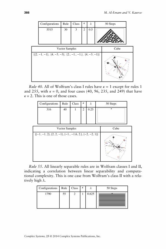
Configurations Rule Class ( & 50 Steps

5515 30 3 2 0.5

Vector Samples Cube

))2, ,1, ,1*, )4, ,3, ,3*, )2., ,1., ,1.*, )4, ,3, ,1**

Rule 40. All of Wolfram#s class I rules have ( ' 1 except for rules 1and 255, with ( ' 0, and four cases (40, 96, 235, and 249) that have( = 2. This is one of those cases.


316 40 1 2 0.25

Vector Samples Cube

)),1, ,1, 2*, )2, 2, ,1*, ),1., ,1.6, 2.*, ),2, ,2, 1**

Rule 55. All linearly separable rules are in Wolfram classes I and II,indicating a correlation between linear separability and computa-tional complexity. This is one case from Wolfram#s class II with a rela-tively high &.


1790 55 2 1 0.625



Vector Samples Cube

))1, 2, 1*, )2, 3, 1*, )2.6, 3.8, 0.2*, )1, 3, 1**

Rule 110. Wolfram#s class IV rules always have ( ' 2. Rule 110 isa clear example for this case.


3854 110 4 2 0.625

Vector Samples Cube

))1, 3, ,4*, )1, ,4, 3*, )0.2, ,1.6, 1.4*, )1, 3, ,4**

Rule 147. This is another clear example for class IV.


4091 147 4 2 0.5

Vector Samples Cube

))1, 2, 1*, )3, 4, 3*, )0.8, 1.4, 0.8*, )3, 4, 3**



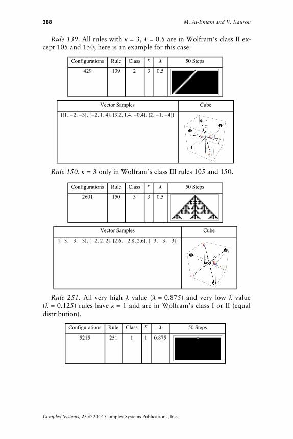
Rule 139. All rules with ( ' 3, & ' 0.5 are in Wolfram#s class II ex-cept 105 and 150; here is an example for this case.


429 139 2 3 0.5

Vector Samples Cube

))1, ,2, ,3*, ),2, 1, 4*, )3.2, 1.4, ,0.4*, )2, ,1, ,4**

Rule 150. ( ' 3 only in Wolfram#s class III rules 105 and 150.


2601 150 3 3 0.5

Vector Samples Cube

)),3, ,3, ,3*, ),2, 2, 2*, )2.6, ,2.8, 2.6*, ),3, ,3, ,3**

Rule 251. All very high & value (& ' 0.875) and very low & value(& ' 0.125) rules have ( ' 1 and are in Wolfram#s class I or II (equaldistribution).


5215 251 1 1 0.875



Vector Samples Cube

)),3, 3, ,3*, ),3, 3, ,2*, ),2.8, 2.6, ,2.8*, ),1, 2, ,1**

Conclusion6.

This paper reports a detailed survey of various complexity measure-ment approaches. It should be clear that there is no measure of com-plexity appropriate to evolution in general, but that it is desirable tobe clear about the language of representation, the type of difficulty,and the overall formulation to which each variety refers. At the veryleast, we should distinguish concepts like size, order, and variety fromcomplexity. In this way, we can be clearer about the strength and con-text of any such use for analysis and communication.

Acknowledgments

Part of this work was performed during my project !An Investigationof the Relation between Nonlinear Dynamical Systems and Elemen-tary Cellular Automata." I am grateful to T. Rowland and V. Kaurovfor mentorship and advice at the Wolfram Science Summer School2012. Valuable discussions with M. Daif and M. Attia are gratefullyacknowledged. I am indebted to T. Rowland for carefully reading anearlier version of this manuscript.



Appendix

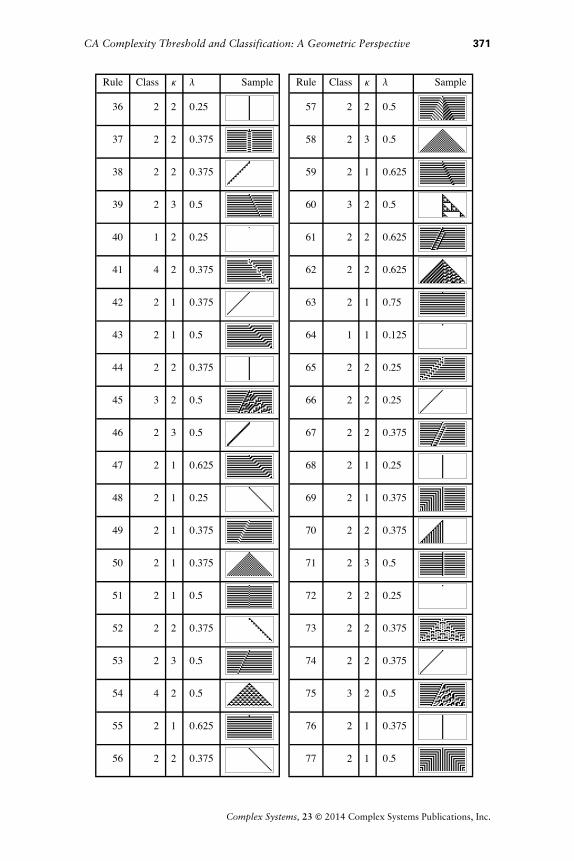
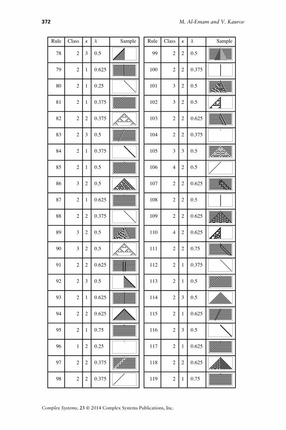
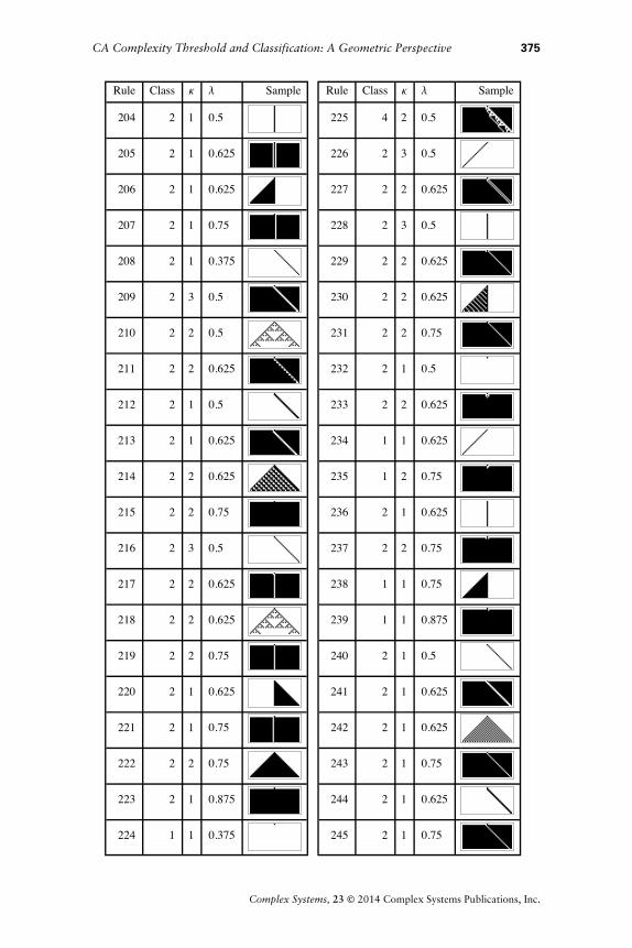
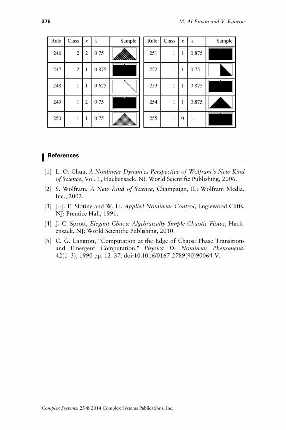
List of ClassificationsA.

Rule Class ( & Sample

0 1 0 0.

1 2 1 0.125

2 2 1 0.125

3 2 1 0.25

4 2 1 0.125

5 2 1 0.25

6 2 2 0.25

7 2 1 0.375

8 1 1 0.125

9 2 2 0.25

10 2 1 0.25

11 2 1 0.375

12 2 1 0.25

13 2 1 0.375

14 2 1 0.375

15 2 1 0.5

16 2 1 0.125

17 2 1 0.25


18 3 2 0.25

19 2 1 0.375

20 2 2 0.25

21 2 1 0.375

22 3 2 0.375

23 2 1 0.5

24 2 2 0.25

25 2 2 0.375

26 2 2 0.375

27 2 3 0.5

28 2 2 0.375

29 2 3 0.5

30 3 2 0.5

31 2 1 0.625

32 1 1 0.125

33 2 2 0.25

34 2 1 0.25

35 2 1 0.375




36 2 2 0.25

37 2 2 0.375

38 2 2 0.375

39 2 3 0.5

40 1 2 0.25

41 4 2 0.375

42 2 1 0.375

43 2 1 0.5

44 2 2 0.375

45 3 2 0.5

46 2 3 0.5

47 2 1 0.625

48 2 1 0.25

49 2 1 0.375

50 2 1 0.375

51 2 1 0.5

52 2 2 0.375

53 2 3 0.5

54 4 2 0.5

55 2 1 0.625

56 2 2 0.375


57 2 2 0.5

58 2 3 0.5

59 2 1 0.625

60 3 2 0.5

61 2 2 0.625

62 2 2 0.625

63 2 1 0.75

64 1 1 0.125

65 2 2 0.25

66 2 2 0.25

67 2 2 0.375

68 2 1 0.25

69 2 1 0.375

70 2 2 0.375

71 2 3 0.5

72 2 2 0.25

73 2 2 0.375

74 2 2 0.375

75 3 2 0.5

76 2 1 0.375

77 2 1 0.5




78 2 3 0.5

79 2 1 0.625

80 2 1 0.25

81 2 1 0.375

82 2 2 0.375

83 2 3 0.5

84 2 1 0.375

85 2 1 0.5

86 3 2 0.5

87 2 1 0.625

88 2 2 0.375

89 3 2 0.5

90 3 2 0.5

91 2 2 0.625

92 2 3 0.5

93 2 1 0.625

94 2 2 0.625

95 2 1 0.75

96 1 2 0.25

97 2 2 0.375

98 2 2 0.375


99 2 2 0.5

100 2 2 0.375

101 3 2 0.5

102 3 2 0.5

103 2 2 0.625

104 2 2 0.375

105 3 3 0.5

106 4 2 0.5

107 2 2 0.625

108 2 2 0.5

109 2 2 0.625

110 4 2 0.625

111 2 2 0.75

112 2 1 0.375

113 2 1 0.5

114 2 3 0.5

115 2 1 0.625

116 2 3 0.5

117 2 1 0.625

118 2 2 0.625

119 2 1 0.75




120 4 2 0.5

121 4 2 0.625

122 3 2 0.625

123 2 2 0.75

124 4 2 0.625

125 2 2 0.75

126 3 2 0.75

127 2 1 0.875

128 1 1 0.125

129 3 2 0.25

130 2 2 0.25

131 2 2 0.375

132 2 2 0.25

133 2 2 0.375

134 2 2 0.375

135 3 2 0.5

136 1 1 0.25

137 4 2 0.375

138 2 1 0.375

139 2 3 0.5

140 2 1 0.375


141 2 3 0.5

142 2 1 0.5

143 2 1 0.625

144 2 2 0.25

145 2 2 0.375

146 3 2 0.375

147 4 2 0.5

148 2 2 0.375

149 3 2 0.5

150 3 3 0.5

151 3 2 0.625

152 2 2 0.375

153 3 2 0.5

154 2 2 0.5

155 2 2 0.625

156 2 2 0.5

157 2 2 0.625

158 2 2 0.625

159 2 2 0.75

160 1 1 0.25

161 3 2 0.375




162 2 1 0.375

163 2 3 0.5

164 2 2 0.375

165 3 2 0.5

166 2 2 0.5

167 2 2 0.625

168 1 1 0.375

169 4 2 0.5

170 2 1 0.5

171 2 1 0.625

172 2 3 0.5

173 2 2 0.625

174 2 1 0.625

175 2 1 0.75

176 2 1 0.375

177 2 3 0.5

178 2 1 0.5

179 2 1 0.625

180 2 2 0.5

181 2 2 0.625

182 3 2 0.625


183 3 2 0.75

184 2 3 0.5

185 2 2 0.625

186 2 1 0.625

187 2 1 0.75

188 2 2 0.625

189 2 2 0.75

190 2 2 0.75

191 2 1 0.875

192 1 1 0.25

193 4 2 0.375

194 2 2 0.375

195 3 2 0.5

196 2 1 0.375

197 2 3 0.5

198 2 2 0.5

199 2 2 0.625

200 2 1 0.375

201 2 2 0.5

202 2 3 0.5

203 2 2 0.625




204 2 1 0.5

205 2 1 0.625

206 2 1 0.625

207 2 1 0.75

208 2 1 0.375

209 2 3 0.5

210 2 2 0.5

211 2 2 0.625

212 2 1 0.5

213 2 1 0.625

214 2 2 0.625

215 2 2 0.75

216 2 3 0.5

217 2 2 0.625

218 2 2 0.625

219 2 2 0.75

220 2 1 0.625

221 2 1 0.75

222 2 2 0.75

223 2 1 0.875

224 1 1 0.375


225 4 2 0.5

226 2 3 0.5

227 2 2 0.625

228 2 3 0.5

229 2 2 0.625

230 2 2 0.625

231 2 2 0.75

232 2 1 0.5

233 2 2 0.625

234 1 1 0.625

235 1 2 0.75

236 2 1 0.625

237 2 2 0.75

238 1 1 0.75

239 1 1 0.875

240 2 1 0.5

241 2 1 0.625

242 2 1 0.625

243 2 1 0.75

244 2 1 0.625

245 2 1 0.75




246 2 2 0.75

247 2 1 0.875

248 1 1 0.625

249 1 2 0.75

250 1 1 0.75


251 1 1 0.875

252 1 1 0.75

253 1 1 0.875

254 1 1 0.875

255 1 0 1.

References

[1] L. O. Chua, A Nonlinear Dynamics Perspective of Wolfram#s New Kindof Science, Vol. 1, Hackensack, NJ: World Scientific Publishing, 2006.

[2] S. Wolfram, A New Kind of Science, Champaign, IL: Wolfram Media,Inc., 2002.

[3] J.-J. E. Slotine and W. Li, Applied Nonlinear Control, Englewood Cliffs,NJ: Prentice Hall, 1991.

[4] J. C. Sprott, Elegant Chaos: Algebraically Simple Chaotic Flows, Hack-ensack, NJ: World Scientific Publishing, 2010.

[5] C. G. Langton, !Computation at the Edge of Chaos: Phase Transitionsand Emergent Computation," Physica D: Nonlinear Phenomena,42(1–3), 1990 pp. 12–37. doi:10.1016/0167-2789(90)90064-V.



Documents

Cellular Automata Complexity Threshold and Classification