CellTracerCellTracer 1.0 Quick Start Guide1.0 Quick Start Guide

Quanli Wang1,3, Lingchong You2,3 and Mike West1,3

1Department of Statistical Science, Duke University2Department of Biomedical Engineering, Duke University3Institute for Genome Sciences & Policy, Duke University

June 2008

1. Install Matlab and Matlab Image Processing Toolbox.

2. Download and unzip CellTracer package to a local directory.

Software environment:

Hardware requirements:1. A computer with faster CPU(s) is preferred due to intensive image

processing operations.

2. Not very demanding on memory usage. Most image data are stored in local drive and are dynamically loaded into memory when necessary.

Prerequisites Prerequisites

Start Start CellTracerCellTracer in in MatlabMatlab

1. Start Matlab and change current working directory to the local directory where CellTracer is installed.

2. Type CellTracer in the Matlab Command Window. You should then see the main CellTracer GUI interface as follows.

General flowchart using General flowchart using CellTracerCellTracer

1. This flowchart gives an overview on how images are processed in CellTracer in an automated way. Not all steps are required for any specific project.

2. Images are first loaded into CellTracerand preprocessed when necessary.

3. User then chooses and applies a set of segmentation tools sequentially to identify blobs such as background, cell border regions and cells.

4. User can manually correct some mistakes from automated segmentation algorithms during step 3.

5. Cell tracking algorithm is then performed when necessary and other tools are also available for data extraction and visualization.

Loading Loading image(simage(s) into ) into CellTracerCellTracer

Click File --> New Project menu to load the image or images from your local drive. You will then see the first image you picked on the left plot panel and you might be prompted to pick a ‘channel’. Just pick one and see what happens and if you are not satisfied , repeat this step to pick another channel. By then you should see something like this. (using the first 5 images from the yeast dataset).

Exploring Images Exploring Images

CellTracer provides a few tools to explore images. You can

• Use the ‘Frame Panel’ to scroll between frames;

• Use the toolbar to zoom in/out and get pixel information.

The screenshot bellow shows a zoomed in image (image 5).

Edit Images Edit Images -- Cropping/Inverting/Double Resolution Cropping/Inverting/Double Resolution

Use the Edit menu items to edit/preprocess input images before segmentation and tracking.

• Edit Crop images into current view menu allows one to focus only on regions of interest in the images.

• Edit Invert Images menu can be useful when the cells have higher than background intensity values. CellTracer usually assumes cells are darker objects in images.

• Edit Double Resolution can be useful when the cells tend to be small. CellTraceruses interpolation to double the image dimension.

• User should only perform these manipulations before segmentation and tracking.

Initial Background Screening Initial Background Screening

Background Identification is usually the first step in cell segmentation. There are a few “background methods” implemented in CellTracer. Here we use the “background—range filtering” method in this demonstration.

• Use Segmentation background—Range Filtering menu to select this method;

• Provide the parameters in the right Parameters panel (as showing in the following screen shot) and then hit the Run button to run the algorithm.

Initial Background Screening Initial Background Screening ----Continued Continued

After running the algorithm, you will see the result in the right plot panel. Backgrounds are represented in green color. And later on, you will also notice that, red color represents the cell borders and blue color represents identified cells.

• The checkboxes in the Parameters panel allow one to apply the selected algorithm on existing result, on all frames or to test the algorithm only.

• The push buttons in the Frame Panel on the bottom-left window allow one to scroll between frames to check result on all frames.

• The overlay tool in the toolbar on the top-left window allows one to overlay results on top of input images to check the result.

• The Border Region /Background and Cell mask tools in the toolbar allow one to manually select and mark regions in the input images as border/background or cells.

• The Object Select tool in the toolbar allows one to select identified regions in the right plot panel.

• One can also use the context menu by right-clicking on selected objects from Object Select tool to perform certain operations in a context-appropriate way.

• The status bar on the bottom would show some basic processing information.

Identifying Border Regions Identifying Border Regions

One can also choose from a few algorithms to identify cell border regions in images. For example:

• Use Segmentation Border—Minimum Ranking menu to select this method;

• Provide the parameters in the right Parameters panel (as showing in the screen shot bellow) and then hit the Run button to run the algorithm.

• The border regions are shown as red in the screen shot bellow.

Identifying Border RegionsIdentifying Border Regions----Continued Continued One can apply the same or different methods sequentially to achieve better results.

For example, here we apply yet another border method to refine the results from previous step.

• Choose Segmentation Border—Rank & Count Transform method;

• Provide the parameters in the right Parameters panel (as showing in the screen shot bellow) and then hit the Run button to run the algorithm.

• The border regions are shown as red in the screen shot bellow.

Identifying CellsIdentifying CellsTwo cell segmentation models and methods are provided in this version. For this

example:

• Choose Segmentation Cell—Convex Model method;

• Provide the parameters in the right Parameters panel (as showing in the screen shot bellow) and then hit the Run button to run the algorithm.

• The cells are shown as blue in the screen shot bellow.

Same plot panelsSame plot panels——different viewsdifferent views

So far, we have only worked on the “Hybrid Images View”, which shows the input grey-scale images on the left plot panel and identified binary masks of different regions on the right panel. Once we have some cell blobs identified, one can also switch to “Segmentation View” or “Tracking View” and manually inspect/correct some mistakes arising from the automated algorithms.

• In “Segmentation View”, the left plot panel shows the input grey-scale image and the right panel shows only the identified cell blobs in random colors. One can use all the available tools from the toolbar to manually add/remove objects and check the segmentation result.

• In “Tracking View”, two consecutive frames are shown in left and right panels to indicate identified cell blobs. One can use the available tools to further correct problems such as removing undesired blobs or manually link/unlink cells from two frames.

• The next two slides will show the “Segmentation View” and “tracking View”respectively.

““Segmentation ViewSegmentation View””

• View Segmentation

• Tip: One can remove the undesired objects in above window by selecting them and right-clicking to get the context menu and then selecting “Removing selected blobs”

““Tracking ViewTracking View””

• View Tracking

• Tip: One can remove the undesired objects in above window by selecting them and right-clicking to get the context menu and then selecting “Removing selected blobs”

• Tip: one can manually link/unlink cells from two frames shown by selecting them and right-clicking to get the context menu then selecting “link/unlink objects”.

Cell TrackingCell Tracking——Global Shift Correction Global Shift Correction

Once the segmentation steps are complete, one can go to next step to apply the cell tracking method. But sometimes it is helpful to do a “Global Shit Correction” before applying the cell tracking algorithm.

• In tracking view, one can apply the overlay tool from the toolbar to see if there is evidence of “global shifting” between frames.

• If one decides there is evidence of “global shifting” , one can correct this by choosing menu “Tracking Global Alignment “and provide the maximum shit parameter then run the algorithm by hitting the Run button.

• After the correction, applying the overlay tool again will show corrected overlapping result.

Cell Tracking Cell Tracking

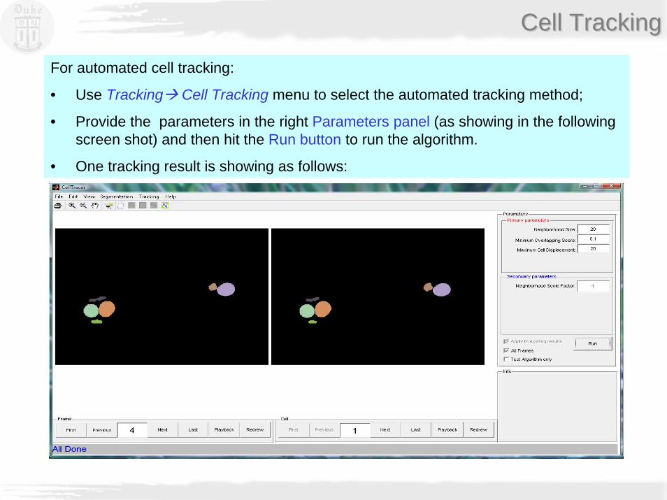
For automated cell tracking:

• Use Tracking Cell Tracking menu to select the automated tracking method;

• Provide the parameters in the right Parameters panel (as showing in the following screen shot) and then hit the Run button to run the algorithm.

• One tracking result is showing as follows:

File Menu File Menu

• Project can be saved and reloaded.

• Currently, the program can take snapshots to save partial results and restore the program from stored snapshots. A more advanced undo/redo implementation will be introduced in a later version.