Embed Size (px)
Citation preview

Brown University
Doctoral Thesis
Celestial Amplitudes Cluster Adjacency and
Symbol Alphabets
Author
Anders Oslashhrberg Schreiber
Supervisor
Prof Anastasia Volovich
A dissertaton submitted in partial fulfillment of the requirements for
the degree of Doctor of Philosophy
in the
Department of Physics at Brown University
Providence Rhode Island
February 2021
copy Copyright 2020 by Anders Oslashhrberg Schreiber
iii
This dissertation by Anders Oslashhrberg Schreiber is accepted in its present form by
the Department of Physics as satisfying the
dissertation requirement for the degree of
Doctor of Philosophy
Date
Anastasia Volovich Advisor
Recommended to the Graduate Council
Date
Antal Jevicki Reader
Date
Chung-I Tan Reader
Approved by the Graduate Council
Date
Andrew G Campbell
Dean of the Graduate School
iv
ldquoAll we have to decide is what to do with the time that is given to usrdquo
mdash JRR Tolkien The Fellowship of the Ring
v
BROWN UNIVERSITY
Abstract
Anastasia Volovich
Department of Physics at Brown University
Doctor of Philosophy
Celestial Amplitudes Cluster Adjacency and Symbol Alphabets
by Anders Oslashhrberg Schreiber
In this thesis we present studies of scattering amplitudes on the celestial sphere at null
infinity (celestial amplitudes) the cluster adjacency structure of scattering amplitudes in
planar maximally supersymmetric Yang-Mills theory (N = 4 SYM) and a method to derive
symbol letters for loop amplitudes in N = 4 SYM
First we show that n-particle celestial gluon tree amplitudes take the form of Aomoto-
Gelfand hypergeometric functions and Gelfand A-hypergeometric functions We then study
conformal properties conformal partial wave decomposition and the optical theorem of
four-particle celestial amplitudes in massless scalar φ3 theory and Yang-Mills theory Sub-
sequently we derive single- and multi-soft theorems for celestial amplitudes in Yang-Mills
theory
Second we provide computational evidence that each rational Yangian invariant inN = 4
SYM has poles that are cluster adjacent (belong to the same cluster in the Gr(4 n) cluster
algebra) through the Sklyanin bracket test We also use this bracket test to study cluster
adjacency of the symbol of one-loop NMHV amplitudes in N = 4 SYM
Finally we suggest an algorithm for computing symbol alphabets from plabic graphs
by solving matrix equations of the form C sdot Z = 0 to associate functions on Gr(mn) to
parameterizations of certain cells in Gr(kn) indexed by plabic graphs For m = 4 and n = 8
vi
we show that this association precisely reproduces the 18 algebraic symbol letters of the
two-loop NMHV eight-particle amplitude from four plabic graphs
vii
Curriculum Vitae
Anders Oslashhrberg Schreiber
Contact and Date of Birth
Date of birth 30 March 1992Country of Citizenship DenmarkAddress Physics Department Barus and Holley Building
Brown University 182 Hope Street Providence RI 02912Phone +1 401 480 3895Email anders_schreiberbrownedu
Research
Dec 2020 - Dec 2021 Postdoctoral Research Associate at University of OxfordPostdoc at the Mathematical Institute under the grant Scattering Ampli-tudes and the Galois Theory of Periods
Jun 2018 - Dec 2020 Research Assistantship at Brown UniversityResearch assistant working under Prof Anastasia Volovich on mathematicalaspects of scattering amplitudes
Education
Feb 2021 PhD in PhysicsBrown University
Aug 2016 Masterrsquos Degree in Physics at the Niels Bohr InstituteUniversity of Copenhagen
Jan 2015 Bachelorrsquos Degree in Physics at the Niels Bohr InstituteUniversity of Copenhagen
May 2014 Exchange Abroad ProgramUniversity of California Berkeley
viii
Teaching
Sep 2016 - May 2018 Teaching assistant at Brown UniversityTaught introductory labs in Physics 0070 Physics 0040 and problem solvingworkshops in Physics 0070
Sep 2014 - Jun 2016 Teaching assistant at The Niels Bohr Institute CopenhagenTaught labs in Electrodynamics 2 and Quantum Mechanics 1 and taught ex-ercise classes in Statistical Physics and Mathematics for Physicists 1 and 2
Jun 2014 - Aug 2014 Physics Teacher at Herning Gymnasium HerningTaught a high school physics B level class in the High School SupplementaryCourse program Teaching involved lectures experimental work correctingproblem sets and experimental reports and examining students an oral final
List of Publications
This thesis is based on the following publications
Jul 2020 ldquoSymbol Alphabets from Plabic Graphswith Jorge Mago Marcus Spradlin and Anastasia VolovichJHEP 10 128 (2020) [arXiv200700646]
May 2020 ldquoA Note on One-loop Cluster Adjacency in N = 4 SYMwith Jorge Mago Marcus Spradlin and Anastasia VolovichAccepted for publication in JHEP [arXiv200507177]
Jun 2019 ldquoYangian Invariants and Cluster Adjacency in N=4 Yang-Millswith Jorge Mago Marcus Spradlin and Anastasia VolovichJHEP 1910 099 (2019) [arXiv190610682]
Apr 2019 ldquoCelestial Amplitudes Conformal Partial Waves and Soft Limitswith Dhritiman Nandan Anastasia Volovich and Michael ZlotnikovJHEP 1910 018 (2019) [arXiv190410940]
Nov 2017 ldquoTree-level gluon amplitudes on the celestial spherewith Anastasia Volovich and Michael ZlotnikovPhys Lett B 781 349 (2018) [arXiv171108435]
ix
Awards Scholarships and Fellowships
May 2020 Physics Merit Fellowship from Brown University Department of Physics
May 2017 Excellence as a Graduate Teaching Assistant from Brown University Depart-ment of Physics
May 2017 Samuel Miller Research Scholarship from the Sigma Alpha Mu Foundation
Schools and Talks
Sep 2020 Conference talk at the DESY Virtual Theory Forum 2020Plabic Graphs and Symbol Alphabets in N=4 super-Yang-Mills Theory
Jan 2020 GGI Lectures on the Theory of Fundamental Interactions
Jan 2020 HET Seminar at NBICluster Adjacency in N=4 Super Yang-Mills Theory
Jul 2019 Poster at Amplitudes 2019Scattering Amplitudes on the Celestial Sphere
Jun 2019 TASI 2019
Jan 2017 Nordic Winter School on Cosmology and Particle Physics 2017
Additional Skills
Languages Danish English German
Computer Literacy MS Windows MS Office LATEX Python Matlab Mathematica
xi
Acknowledgements
The journey of my PhD has been fantastic I have faced many challenges but a lot
of people have been there to help and guide me through these Firstly I would like to
thank my advisor Anastasia Volovich who has been tremendously helpful in making me
grow as a physicist I am grateful for your patience support and guidance throughout my
graduate studies I would also like to thank the other professors in the high energy theory
group including Stephon Alexander Ji Ji Fan Herb Fried Jim Gates Antal Jevicki Savvas
Koushiappas David Lowe Marcus Spradlin and Chung-I Tan You have all stimulated
a rich and exciting research environment on the fifth floor of Barus and Holley and have
made it a pleasure to work in your group I would like to especially thank Antal Jevicki and
Chung-I Tan for being on my thesis committee Thank you also to the postdocs in the high
energy theory group over the years including Cheng Peng Giulio Salvatori David Ramirez
JJ Stankowicz and Akshay Yelleshpur Srikant I have learned a lot from my discussions
with all of you Finally I would like to thank Idalina Alarcon Barbara Cole Mary Ann
Rotondo Mary Ellen Woycik You have all made my life in the physics department infinitely
easier and I have enjoyed the many conversations we have had
I would now like to thank all the other students in the high energy theory group that I
have had the pleasure to work alongside with during my PhD Thank you all for being good
friends and supporting me on my journey Jatan Buch Atreya Chatterjee Tom Harrington
Yangrui Crystal Hu Leah Jenks Michael Toomey Shing Chau John Leung Luke Lippstreu
Sze Ning Hazel Mak Igor Prlina Lecheng Ren Robert Sims Stefan Stanojevic Kenta
Suzuki Jorge Leonardo Mago Trejo and Peter Tsang
xii
I have spent a large chunk of my free time in the Nelson Fitness Center throughout my
PhD where I have enjoyed training for powerlifting I would like to thank all my fellow
lifters in from the Nelson and in the Brown Barbell Club All of you have lifted me up to
be a better powerlifter
I am so thankful for my lovely girlfriend Nicole Ozdowski Thank you for being there for
me and supporting me every day Big thanks to my parents Per Schreiber Tina Schreiber
my brother Jesper Schreiber my grandparents Lizzie Pedersen Bodil Schreiber and Karl-
Johan Schreiber who have been my biggest supporters from day one
Finally I would like to thank all the people I have not listed here I have met so many
people at Brown over the years and you have all had a positive impact on my life and my
journey towards PhD Thank you all
xiii
Contents
Abstract v
Acknowledgements xi
1 Introduction 1
11 Celestial Amplitudes and Holography 3
111 Conformal Primary Wavefunctions 3
112 Celestial Amplitudes 4
12 Cluster Algebras in planar N = 4 super Yang-Mills Theory 6
121 Momentum Twistors and Dual Conformal Symmetry 6
122 Cluster Algebras and Cluster Adjacency 8
13 Symbols Alphabet and Plabic Graphs 10
131 Yangian Invariants and Leading Singularities 11
132 Plabic Graphs and Cluster Algebras 11
2 Tree-level Gluon Amplitudes on the Celestial Sphere 15
21 Gluon amplitudes on the celestial sphere 17
22 n-point MHV 19
221 Integrating out one ωi 19
xiv
222 Integrating out momentum conservation δ-functions 20
223 Integrating the remaining ωi 22
224 6-point MHV 24
23 n-point NMHV 25
24 n-point NkMHV 28
25 Generalized hypergeometric functions 31
3 Celestial Amplitudes Conformal Partial Waves and Soft Limits 35
31 Scalar Four-Point Amplitude 37
32 Gluon Four-Point Amplitude 42
33 Soft limits 43
34 Conformal Partial Wave Decomposition 47
35 Inner Product Integral 49
4 Yangian Invariants and Cluster Adjacency in N = 4 Yang-Mills 53
41 Cluster Coordinates and the Sklyanin Poisson Bracket 56
42 An Adjacency Test for Yangian Invariants 58
421 NMHV 60
422 N2MHV 62
423 N3MHV and Higher 63
43 Explicit Matrices for k = 2 64
5 A Note on One-loop Cluster Adjacency in N = 4 SYM 69
51 Cluster Adjacency and the Sklyanin Bracket 70
xv
52 One-loop Amplitudes 73
521 BDS- and BDS-like Subtracted Amplitudes 73
522 NMHV Amplitudes 75
53 Cluster Adjacency of One-Loop NMHV Amplitudes 76
531 The Symbol and Steinmann Cluster Adjacency 76
532 Final Entry and Yangian Invariant Cluster Adjacency 76
54 Cluster Adjacency and Weak Separation 79
55 n-point NMHV Transcendental Functions 82
6 Symbol Alphabets from Plabic Graphs 85
61 A Motivational Example 87
62 Six-Particle Cluster Variables 91
63 Towards Non-Cluster Variables 95
64 Algebraic Eight-Particle Symbol Letters 98
65 Discussion 101
66 Some Six-Particle Details 104
67 Notation for Algebraic Eight-Particle Symbol Letters 105
xvii
List of Figures
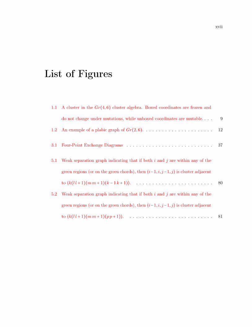
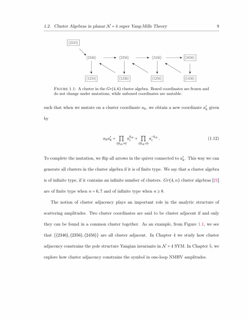
11 A cluster in the Gr(46) cluster algebra Boxed coordinates are frozen and
do not change under mutations while unboxed coordinates are mutable 9
12 An example of a plabic graph of Gr(26) 12
31 Four-Point Exchange Diagrams 37
51 Weak separation graph indicating that if both i and j are within any of the
green regions (or on the green chords) then ⟨iminus1 i jminus1 j⟩ is cluster adjacent
to ⟨k(l l + 1)(mm + 1)(k minus 1k + 1)⟩ 80
52 Weak separation graph indicating that if both i and j are within any of the
green regions (or on the green chords) then ⟨iminus1 i jminus1 j⟩ is cluster adjacent
to ⟨k(l l + 1)(mm + 1)(pp + 1)⟩ 81
xviii
61 The three types of (reduced perfectly orientable bipartite) plabic graphs
corresponding to km-dimensional cells of Gr(kn)ge0 for k = 2 m = 4 and
n = 6 are shown in (a)ndash(c) The associated input and output clusters (see
text) are shown in (d)ndash(f) and (g)ndash(i) respectively Lines connecting two
frozen nodes are usually omitted but we include in (g)ndash(i) the dotted lines
(having ldquoblack on the rightrdquo in the dual plabic graph) that encode (66) (627)
and (629) (up to signs) 93
xix
List of Tables
xxi
Dedicated to my family Tina Per Jesper Lizzie Bodil and Karl-Johan
I love you all
1
Chapter 1
Introduction
The study of elementary particles and their interactions have led to a paradigm shift in our
understanding of the laws of nature in the past 100 years From early discoveries of charged
particles in cloud chambers to deep probing of the structure of hadrons in high powered
particle accelerators we today have an incredible understanding of how the universe works
through the Standard Model of particle physics The enormous success of the Standard
Model of particle physics is hinged on our ability to calculate scattering cross sections which
we measure in particle scattering experiments like the Large Hadron Collider (LHC) The
computation of scattering cross sections in turn depend on our ability to compute scattering
amplitudes
When we are taught quantum field theory in graduate school we learn the method of
Feynman diagrams [1] to compute scattering amplitudes This method originally revolu-
tionized the way one thinks about scattering in quantum field theories as it gives a neat
way to organize computations via simple diagrams However computations of scattering
amplitudes via Feynman diagrams have rapidly scaling complexity with the number of par-
ticles involved in the scattering process For example if we consider 2-to-n gluon scattering
2 Chapter 1 Introduction
at tree level in Yang-Mills theory the following number of Feynman diagrams need to be
calculated
g + g rarr g + g 4 diagrams
g + g rarr g + g + g 25 diagrams
g + g rarr g + g + g + g 220 diagrams
However amplitudes often enjoy dramatic simplifications once all the diagrams are added
up A classic example of this is the Parke-Taylor formula [2] for maximally helicity violating
(MHV) scattering of any number of particles This reduction in complexity hints at hidden
simplicity and potentially more efficient techniques for computing amplitudes
To understand and develop new computational techniques we need to understand the
analytic structure of amplitudes We therefore study amplitudes in various bases and vari-
ables as this can highlight special properties The choice of basis states of external particles
can make various symmetry properties of amplitudes manifest Certain kinematic variables
offer simplifications like in the Parke-Taylor formula but also highlight deeper properties
of the amplitudes like dual superconformal symmetry [3] and when utilizing momentum
twistors [4] cluster algebraic structure [5] in planar maximally supersymmetric Yang-Mills
theory (N = 4 SYM) becomes apparent
In the next three sections we review the three main topics of this thesis scattering
amplitudes on the celestial sphere at null infinity of flat space cluster adjacency in scattering
amplitudes in N = 4 SYM and the determination of symbol alphabets of loop amplitudes
in N = 4 SYM via plabic graphs
11 Celestial Amplitudes and Holography 3
11 Celestial Amplitudes and Holography
In the last 23 years theoretical physics has seen a paradigm shift with the introduction of
the anti-de Sitter spaceconformal field theory (AdSCFT) holographic principle [6] Here
observables of string theories in the bulk of the AdS are dual to observables of CFTs that
live on the boundary of AdS This principle has a strongweak coupling duality where for
example observables in the bulk theory at weak coupling are dual to observables of the
boundary CFT at strong coupling This offers a powerful tool as we can use perturbation
theory at weak coupling to do computations and get results in theories at strong coupling
via the duality In flat Minkowski space a similar connection was observed in [7] as it is
possible to slice Minkowski space in four dimensions into slices of AdS3 where one can apply
the tools of AdSCFT This has recently lead to an application in scattering amplitudes in
flat space [8] where it is possible to map plane-waves to the celestial sphere at null infinity
via conformal primary wavefunctions [9]
111 Conformal Primary Wavefunctions
When we compute scattering amplitudes in flat space the initial and final states are chosen
in the basis of plane-waves eplusmniksdotX (for scalars) The plane-wave basis makes translation
symmetry manifest while other features like boosts are obscured A new basis called
conformal primary wavefunctions was introduced in [9] These wavefunctions connect plane-
wave representations of particle wavefunctions at a point in flat space Xmicro to a point on the
celestial sphere at null infinity (z z) (in stereographic coordinates) For a massless scalar
4 Chapter 1 Introduction
particle the conformal primary wavefunction takes the form of a Mellin transform
φ∆plusmn(X z z) = intinfin
0dω ω∆minus1eplusmniωqsdotX (11)
where ∆ is a free parameter that will take the role of conformal dimension By requiring φ to
form an orthonormal basis with respect to the Klein-Gordon inner product ∆ is restricted to
the principal series ∆ = 1+iλ In the above formula we have parameterized the momentum
associated with the massless scalar as
kmicro = ωqmicro(z z) = ω(1 + zz z + zminusi(z minus z)1 minus zz) (12)
where qmicro is a null vector In four dimensions Lorentz transformations act as two-dimensional
conformal transformations on the celestial sphere [10] and under Lorentz transformations
(11) transforms as
φ∆plusmn (ΛmicroνXν az + bcz + d
az + bcz + d
) = ∣cz + d∣2∆φ∆plusmn(X z z) (13)
which is exactly how scalar conformal primaries transform The formula (11) extends to
massless spinning particles of integer spin given by a Mellin transform of the associated
polarization vector and plane-wave [9]
112 Celestial Amplitudes
Given a scattering amplitudes we can change the basis to conformal primary wavefunctions
by applying a Mellin transform to each external particle involved in the scattering process
11 Celestial Amplitudes and Holography 5
This defines the celestial amplitude [9]
AJ1⋯Jn(∆j zj zj) =n
prodj=1int
infin
0dωj ω
∆jminus1j A`1⋯`n (14)
where `j is helicity of particle j and Jj is the spin of the associated conformal primary
wavefunction given by Jj = `j Note that the scattering amplitude A here includes the
overall momentum conservation delta function The celestial amplitude transforms as a
conformal correlator under SL(2C) Lorentz transformations
AJ1⋯Jn (∆j az + bcz + d
az + bcz + d
) =n
prodj=1
[(czj + d)∆j+Jj(cz + d)∆jminusJj ] AJ1⋯Jn(∆j zj zj) (15)
Due to the conformal correlator nature of celestial amplitudes it is possible that there exists
a conformal field theory on the celestial sphere that generates scattering amplitudes in the
form of celestial amplitudes In Chapter 2 we will explore how to compute n-point celestial
gluon amplitudes
In Chapter 3 we will explore conformal properties of four-point massless scalar celestial
amplitudes conformal partial wave decomposition and optical theorem For four-point
celestial gluon amplitudes we compute the conformal partial wave decomposition and study
single- and multi-soft theorems
6 Chapter 1 Introduction
12 Cluster Algebras in planar N = 4 super Yang-Mills Theory
Theories with a large amount of symmetry often see fruitful developments from studying
them in terms of different kinematic variables We will study N = 4 SYM which enjoys su-
perconformal symmetry in spacetime in addition to dual superconformal symmetry in dual
momentum space [3] When kinematics are parameterized in terms of momentum twistors
[4] n-points on P3 dual conformal symmetry enhances the kinematic space to the Grassman-
nian Gr(4 n) [5] This space has a cluster algebraic structure which strongly constrains the
analytic structure of amplitudes in the theory At tree-level amplitudes in N = 4 SYM are
rational functions depending on dual superconformally invariant combinations of momen-
tum twistors called Yangian invariants [11] At loop-level trancendental functions appear
which in the cases of our interest can be described by iterated integrals called generalized
polylogarithms These have a total differential given by a product of d logrsquos which can be
mapped to a tensor product structure called the symbol [12] The structure of both Yangian
invariants and symbols is constrained by cluster adjacency which we will describe below
Cluster adjacency has been used to perform computations of high loop amplitudes in the
cluster bootstrap program [13]
121 Momentum Twistors and Dual Conformal Symmetry
Dual conformal symmetry [3] in N = 4 SYM was discovered by studying scattering ampli-
tudes in dual momentum space We start with scattering amplitudes described by momenta
12 Cluster Algebras in planar N = 4 super Yang-Mills Theory 7
kmicroi of massless particles We define dual momenta xmicroi as
kmicroi = xmicroi minus x
microi+1 (16)
where the index i labels particles i isin 1 n in an ordered fashion Let us now define a
second set of coordinates called momentum twistors [4] We can define these through inci-
dence relations Since we are considering massless particles the definition of dual momenta
combined with the spinor-helicity formalism (see [14] for a review) allows us to write (16)
as
⟨i∣axaai = ⟨i∣axaai+1 equiv [microi∣a (17)
We can pair the momentum twistor components [microi∣a with the spinor-helicity angle bracket
to form a joint spinor that we will collectively refer to as a momentum twistor
ZIi = (∣i⟩a [microi∣a) (18)
where I = (a a) is an SU(22) index As the momentum twistor is defined from two points in
dual momentum space this definition maps any two null separated points in dual momentum
space to a point in momentum twistor space With a bit of algebra we can write point in
dual momentum in terms of the momentum twistor variables
xaai = ∣i⟩a[microiminus1∣a minus ∣i minus 1⟩a[microi∣a⟨i minus 1 i⟩ (19)
8 Chapter 1 Introduction
Due to the construction of the momentum twistor variables via (17) all coordinates in
the momentum twistor ZIi scales uniformly under little group transformations Thus for
n-particle scattering the kinematic space is n-points on P3 also known as twistor space
[15 16] Furthermore dual conformal transformations act as GL(4) transformations on
momentum twistors thus enhancing the momentum twistors from living in P3 to Gr(4 n)
Dual conformal generators act linearly on functions of momentum twistors and we can
construct a dual conformally invariant quantity from the SU(22) Levi-Civita symbol
⟨ijkl⟩ = εIJKLZIi ZJj ZKk ZLl (110)
which will be the central objects that we construct scattering amplitudes from
122 Cluster Algebras and Cluster Adjacency
Cluster algebras [17 18 19 20] can be represented by quivers with cluster coordinates (each
quiver corresponding to a single cluster) equipped with a mutation rule Starting with an
initial cluster we can mutate on individual cluster coordinates and obtain different clusters
As an example consider a cluster in the Gr(46) cluster algebra Figure 11 Here we have
frozen coordinates (in boxes) that we are not allowed to mutate and non-frozen coordinates
(unboxed) that we can mutate on The mutation rule is defined by an adjacency matrix
bij = ( arrows irarr j) minus ( arrows j rarr i) (111)
12 Cluster Algebras in planar N = 4 super Yang-Mills Theory 9
〈2345〉
〈2346〉 〈2356〉 〈2456〉 〈3456〉
〈1234〉 〈1236〉 〈1256〉 〈1456〉
Figure 11 A cluster in the Gr(46) cluster algebra Boxed coordinates are frozen anddo not change under mutations while unboxed coordinates are mutable
such that when we mutate on a cluster coordinate ak we obtain a new coordinate aprimek given
by
akaprimek = prod
i∣bikgt0
abiki + prodi∣biklt0
aminusbiki (112)
To complete the mutation we flip all arrows in the quiver connected to aprimek This way we can
generate all clusters in the cluster algebra if it is of finite type We say that a cluster algebra
is of infinite type if it contains an infinite number of clusters Gr(4 n) cluster algebras [21]
are of finite type when n = 67 and of infinite type when n ge 8
The notion of cluster adjacency plays an important role in the analytic structure of
scattering amplitudes Two cluster coordinates are said to be cluster adjacent if and only
they can be found in a common cluster together As an example from Figure 11 we see
that ⟨2346⟩ ⟨2356⟩ ⟨2456⟩ are all cluster adjacent In Chapter 4 we study how cluster
adjacency constrains the pole structure Yangian invariants in N = 4 SYM In Chapter 5 we
explore how cluster adjacency constrains the symbol in one-loop NMHV amplitudes
10 Chapter 1 Introduction
13 Symbols Alphabet and Plabic Graphs
An outstanding problem in the computation of scattering amplitudes of N = 4 SYM is
the determination of symbol alphabets of amplitudes When amplitudes are computed say
via the cluster bootstrap method the symbol alphabet is an important input but it is only
known in certain cases either via cluster algebras [5] or direct computation [22 23 24] From
cluster algebras we are limited to cases where the cluster algebra is of finite type (n = 67)
Is there an alternative way to predict the symbol alphabet of amplitudes in N = 4 SYM
One approach is using Landau analysis [25 26] but here we will discuss a separate approach
involving plabic graphs that index Grassmannian cells Formulas involving integrals over
Grassmannian spaces are commonplace in N = 4 SYM [27 28] Yangian invariants and
leading singularities are computed as integrals over Grassmannian cells indexed by plabic
graphs [29 30] These integral formulas are localized on solutions to matrix equations of the
form C sdotZ = 0 where C is a ktimesn matrix representation of the auxiliary Grassmannian space
Gr(kn) and Z is the collection of 4 times n momentum twistors As these equations together
with the integral formulas determine the structure of Yangian invariants and leading sin-
gularities it is interesting to ask if we can derive complete symbol alphabets of amplitudes
by collecting coordinates appearing in the solutions to C sdotZ = 0
13 Symbols Alphabet and Plabic Graphs 11
131 Yangian Invariants and Leading Singularities
We can represent Yangian invariants in N = 4 SYM as integrals over an auxiliary Grass-
mannian space [27 28]
Y (Z ∣η) = int4k
prodi=1
d log fi4
prodI=1
k
prodα=1
δ(n
suma=1
Cαa(Z ∣η)aI) (113)
where fi are variables parameterizing the k times n matrix C The integration is localized on
solutions to the matrix equations Cαa(Z ∣η)aI equiv C sdot Z = 0 for a = 1 n I = 1 4 and
α = 1 k Here k corresponds to the level of helicity violation of an NkMHV amplitude
For a n we can consider the finite set of all Gr(kn) cells each with an associated matrix
C such that they exactly localize the integration (113) Thus for each Gr(kn) cell there is
a corresponding Yangian invariant where variables appearing in the Yangian invariant are
dictated by the solutions to C sdotZ = 0
132 Plabic Graphs and Cluster Algebras
Cells of Gr(kn) Grassmannians can be indexed by decorated permutations [29] ie per-
mutations σ of length n with σ(a) if a lt σ(a) and σ(a)+n if σ(a) lt a Furthermore k refers
to the number of entries in a permutation with σ(a) lt a Such decorated permutations can
be represented by plabic graphs - planar bicolored graphs [29]
Example Consider the plabic graph in Figure 12 which has an associated decorated
permutation 345678 To read off the permutation we start at any external point
move through the graph turn to the first left path if we meet a white vertex while we turn
to the first right path if we meet a black vertex
12 Chapter 1 Introduction
Figure 12 An example of a plabic graph of Gr(26)
We can read off the C-matrix parameterizing the associated cell in Gr(kn) from the
plabic graph We start with a matrix that has the identity in the columns corresponding to
sources in the plabic graph Each entry in the remaining columns is given by the formula
cij = (minus1)s sump∶i↦j
prodαisinp
fα (114)
where s is the number of sources strictly between i and j the sum runs over all allowed
paths p from i to j (allowed paths must traverse each edge only in the direction of its arrow)
and the product runs over all faces α to the right of the path p denoted by p On top of
this the face variables fi over-count the degrees of freedom in a plabic graph by one and
satisfy the relation
prodi
fi = 1 (115)
With the construction (114) we will study solutions to the matrix equations C sdotZ = 0
13 Symbols Alphabet and Plabic Graphs 13
In Chapter 6 we will see how this method can be used to generate all Gr(4 n) cluster
coordinates when n = 67 (which are known to be the n = 67 symbols alphabets) but also
algebraic coordinates that are known to appear in scattering amplitudes but are not cluster
coordinates
15
Chapter 2
Tree-level Gluon Amplitudes on the
Celestial Sphere
This chapter is based on the publication [31]
The holographic description of bulk physics in terms of a theory living on the boundary
has been concretely realised by the AdSCFT correspondence for spacetimes with global
negative curvature It remains an important outstanding problem to understand suitable
formulations of holography for flat spacetime a goal that has elicited a considerable amount
of work from several complementary approaches [32]
Recently Pasterski Shao and Strominger [8] studied the scattering of particles in four-
dimensional Minkowski space and formulated a prescription that maps these amplitudes to
the celestial sphere at infinity The Lorentz symmetry of four-dimensional Minkowski space
acts as the conformal group SL(2C) on the celestial sphere It has been shown explicitly
that the near-extremal three-point amplitude in massive cubic scalar field theory has the
correct structure to be identified as a three-point correlation function of a conformal field
16 Chapter 2 Tree-level Gluon Amplitudes on the Celestial Sphere
theory living on the celestial sphere [8] The factorization singularities of more general scat-
tering amplitudes in this CFT perspective have been further studied in [33] The map uses
conformal primary wave functions which have been constructed for various fields in arbitrary
dimensions in [9] In [34] it was shown that the change of basis from plane waves to the
conformal primary wave functions is implemented by a Mellin transform which was com-
puted explicitly for three and four-point tree-level gluon amplitudes The optical theorem
in the conformal basis and scattering in three dimensions were studied in [35] One-loop
and two-loop four-point amplitudes have also been considered in [36]
In this note we use the prescription [34] to investigate the structure of CFT correlators
corresponding to arbitrary n-point gluon tree-level scattering amplitudes thus generaliz-
ing their three- and four-point MHV results Gluon amplitudes can be represented in many
different ways that exhibit different complementary aspects of their rich mathematical struc-
ture It is natural to suspect that they may also take a particularly interesting form when
written as correlators on the celestial sphere We find that Mellin transforms of n-point
MHV gluon amplitudes are given by Aomoto-Gelfand generalized hypergeometric functions
on the Grassmannian Gr(4 n) (224) For non-MHV amplitudes the analytic structure of
the resulting functions is more complicated and they are given by Gelfand A-hypergeometric
functions (233) and its generalizations It will be very interesting to explore further the
structure of these functions and possibly make connections to other representations of tree-
level amplitudes [37] which we leave for future work
21 Gluon amplitudes on the celestial sphere 17
21 Gluon amplitudes on the celestial sphere
We work with tree-level n-point scattering amplitudes of massless particlesA`1⋯`n(kmicroj ) which
are functions of external momenta kmicroj and helicities `j = plusmn1 where j = 1 n We want
to map these scattering amplitudes to the celestial sphere To that end we can parametrize
the massless external momenta kmicroj as
kmicroj = εjωjqmicroj equiv εjωj(1 + ∣zj ∣2 zj + zj minusi(zj minus zj)1 minus ∣zj ∣2) (21)
where zj zj are the usual complex cordinates on the celestial sphere εj encodes a particle
as incoming (εj = minus1) or outgoing (εj = +1) and ωj is the angular frequency associated with
the energy of the particle [34] Therefore the amplitude A`1⋯`n(ωj zj zj) is a function of
ωj zj and zj under the parametrization (21)
Usually we write any massless scattering amplitude in terms of spinor-helicity angle-
and square-brackets representing Weyl-spinors (see [14] for a review) The spinor-helicity
variables are related to external momenta kmicroj so that in turn we can express them in terms
of variables on the celestial sphere via [34]
[ij] = 2radicωiωj zij ⟨ij⟩ = minus2εiεj
radicωiωjzij (22)
where zij = zi minus zj and zij = zi minus zj
18 Chapter 2 Tree-level Gluon Amplitudes on the Celestial Sphere
In [9 34] it was proposed that any massless scattering amplitude is mapped to the
celestial sphere via a Mellin transform
AJ1⋯Jn(λj zj zj) =n
prodj=1int
infin
0dωj ω
iλjj A`1⋯`n(ωj zj zj) (23)
The Mellin transform maps a plane wave solution for a helicity `j field in momentum space
to a corresponding conformal primary wave function on the boundary with spin Jj where
helicity `j and spin Jj are mapped onto each other and the operator dimension takes values
in the principal continuous series representation ∆j = 1+iλj [9] Therefore AJ1⋯Jn(λj zj zj)
has the structure of a conformal correlator on the celestial sphere where the symmetry group
of diffeomorphisms is the conformal group SL(2C)
Explicitly under conformal transformations we have the following behavior
ωj rarr ωprimej = ∣czj + d∣2ωj zj rarr zprimej =azj + bczj + d
zj rarr zprimej =azj + bczj + d
(24)
where a b c d isin C and ad minus bc = 1 The transformation for zj zj is familiar from the
usual action of SL(2C) on the complex coordinates on a sphere Concerning ωj recall
that qmicroj transforms as qmicroj rarr ∣czj + d∣minus2Λmicroνqνj [9] where Λmicroν is a Lorentz transformation in
Minkowski space corresponding to the celestial sphere conformal transformation Thus ωj
must transform as in (24) to ensure that kmicroj transforms as a Lorentz vector kmicroj rarr Λmicroνkνj
The conformal covariance of AJ1⋯Jn(λj zj zj) on the celestial sphere demands
AJ1⋯Jn (λj azj + bczj + d
azj + bczj + d
) =n
prodj=1
[(czj + d)∆j+Jj(czj + d)∆jminusJj ] AJ1⋯Jn(λj zj zj) (25)
22 n-point MHV 19
as expected for a correlator of operators with weights ∆j and spins Jj
22 n-point MHV
The cases of 3- and 4-point gluon amplitudes have been considered in [34] Here we will
map n ge 5-point MHV gluon amplitudes to the celestial sphere
221 Integrating out one ωi
Starting from (23) we can anchor the integration to one of our variables ωi by making a
change of variables for all l ne i
ωl rarrωisiωl (26)
where si is a constant factor that cancels the conformal scaling of ωi in (24) so that the
ratio ωi
siis conformally invariant One choice which is always possible in Minkowski signature
is
si =∣ziminus1 i+1∣
∣ziminus1 i∣ ∣zi i+1∣ (27)
Since gluon scattering amplitudes scale homogeneously under uniform rescalings col-
lecting all the factors in front we have
AJ1⋯Jn(λj zj zj) = intinfin
0
dωiωi
(ωisi
)sumn
j=1 iλj
s1+iλii
⎛⎜⎝
n
proda=1anei
intinfin
0dωa ω
iλaa
⎞⎟⎠A`1⋯`n(si ωl zj zj)
(28)
20 Chapter 2 Tree-level Gluon Amplitudes on the Celestial Sphere
where we used that the scaling power of dressed gluon amplitudes is An(Λωi)rarr ΛminusnAn(ωi)
We recognize that the integral over ωi is the Mellin transform of 1 which is given by
intinfin
0
dωiωi
(ωisi
)iz
= 2πδ(z) (29)
With this we simplify the transformation prescription (23) to
AJ1⋯Jn(λj zj zj) = 2πδ⎛⎝n
sumj=1
λj⎞⎠s1+iλii
⎛⎜⎝
n
proda=1anei
intinfin
0dωa ω
iλaa
⎞⎟⎠A`1⋯`n(si ωl zj zj) (210)
222 Integrating out momentum conservation δ-functions
For simplicity we choose the anchor variable above to be ω1 and use ωnminus3 ωn to localize
the momentum conservation δ-functions in the amplitude These δ-functions can then be
equivalently rewritten as follows compensating the transformation by a Jacobian
δ4(ε1s1q1 +n
sumi=2
εiωiqi) =4
U
n
prodj=nminus3
sjδ (ωj minus ωlowastj )1gt0(ωlowastj ) (211)
where ωlowastj are solutions to the initial set of linear equations
ω⋆j = minussj (U1j
U+nminus4
sumi=2
ωisi
Uij
U) (212)
The Uij and U are minor determinants by Cramerrsquos rule
Uij = det(Mnminus3jrarrin) U = det(Mnminus3n) (213)
22 n-point MHV 21
where j rarr i means that index j is replaced by index i Mabcd denotes the 4 times 4 matrix
Mabcd = (pa pb pc pd) (214)
For the purpose of determinant calculation the column vectors pmicroi = εisiqmicroi can be written
in a manifestly conformally invariant form
pmicro1(z z) = ε1(100minus1) pmicro2(z z) = ε2(1001) pmicro3(z z) = ε3(2200)
pmicroi (z z) = εi1
∣ui∣(1 + ∣ui∣2 ui + uiminusi(ui minus ui)1 minus ∣ui∣2) for i = 45 n
(215)
in terms of conformal invariant cross-ratios
ui =z31zi2z32zi1
and ui =z31zi2z32zi1
for i = 45 n (216)
but if and only if we also specify the explicit choice
s1 =∣z32∣
∣z31∣ ∣z12∣ s2 =
∣z31∣∣z32∣ ∣z21∣
and si =∣z12∣
∣z1i∣ ∣zi2∣for i = 3 n (217)
The indicator functions prodni=nminus3 1gt0(ωlowasti ) appear due to the integration range in all ω being
along the positive real line such that the δ-functions can only be localized in this region
Furthermore in order for all the remaining integration variables ωj with j = 2 n minus 4
to be defined on the whole integration range the indicator functions prodni=nminus3 1gt0(ωlowasti ) have
to demand Uij
U lt 0 for all i = 1 n minus 4 and j = n minus 3 n so that we can write them as
prodij 1lt0(Uij
U )
22 Chapter 2 Tree-level Gluon Amplitudes on the Celestial Sphere
223 Integrating the remaining ωi
In this section we apply (210) to the usual n-point MHV Parke-Taylor amplitude [2] in
spinor-helicity formalism for n ge 5 rewritten via (327)
Aminusminus++(s1 ωj zj zj) =z3
12s1ω2δ4(ε1s1q1 +sumni=2 εiωiqi)
(minus2)nminus4z23z34zn1ω3ω4ωn (218)
Making use of the solutions (211) and performing four of the integrations in (210) we have
Aminusminus++(λi zi zi) = 2πδ(sumnj=1 λj)z3
12 siλ1+21
(minus2)nminus4Uz23z34zn1
nminus4
proda=2int
infin
0dωa ω
iλaa
ω2prodnb=nminus3 sbωlowastbiλnminus3
ω3ω4ωlowastnprodij
1lt0(Uij
U)
(219)
For convenience we transform the remaining integration variables as
ωi = siU1n
Uin
uiminus1
1 minussumnminus5j=1 uj
i = 23 n minus 4 (220)
which leads to
Aminusminus++(λi zi zi) simz3
12siλ1+21 siλ2+2
2 siλ33 siλnn
z23z34zn1U1nδ(
n
sumj=1
λj) ϕ(α x)prodij
1lt0(Uij
U) (221)
Note that the overall factor in (221) accounts for proper transformation weight of the
resulting correlator under conformal transformations (25)
22 n-point MHV 23
Here we recognize a hypergeometric function ϕ(α x) of type (n minus 4 n) as defined in
section 381 of [38] and described in appendix 25 In particular here we have
ϕ(α x) equivintu1ge0unminus5ge01minussuma uage0
n
prodj=1
Pj(u)αjdϕ dϕ = dP2
P2and and dPnminus4
Pnminus4
Pj(u) =x0j + x1ju1 + + xnminus5 junminus5 1 le j le n
(222)
The parameters in (222) corresponding to (221) read1
α1 =1 α2 = 2 + iλ2 α3 = iλ3 αnminus4 = iλnminus4 αnminus3 = iλnminus3 minus 1 αnminus1 = iλnminus1 minus 1
αn =1 + iλ1 x0 i =U1i
U1n xjminus1 i =
Uji
Ujnminus U1i
U1n x0n = minus
U
U1n xjminus1n =
U
U1n x01 = 1 xjminus1 j = minus
U
Ujn
(223)
for i = n minus 3 n minus 2 n minus 1 and j = 23 n minus 4 and all other xab = 0
These kinds of functions are also known as Aomoto-Gelfand hypergeometric functions
on the Grassmannian Gr(n minus 4 n)
Making use of eq (324) and (325) from [38] we can write down a dual representation
of the same function which yields a hypergeometric function of type (4 n)
ϕ(α x) equivc2
c1intu1ge0u3ge0
1minussuma uage0
n
prodj=1
Pj(u)αjdϕ dϕ = dPnminus3
Pnminus3and and dPnminus1
Pnminus1
Pj(u) =x0j + x1ju1 + x2ju2 + x3ju3 1 le j le n
(224)
1For n = 5 the normally different cases α2 = 2+iλ2 and αnminus3 = iλnminus3minus1 are reduced to a single α2 = 1+iλ2In this case there also are no integrations so that the result becomes a simple product of factors
24 Chapter 2 Tree-level Gluon Amplitudes on the Celestial Sphere
In this case the parameters of (224) corresponding to (221) read
α1 =1 α2 = minus2 minus iλ2 α3 = minusiλ3 αnminus4 = minusiλnminus4 αnminus3 = 1 minus iλnminus3 αnminus1 = 1 minus iλnminus1
αn = minus iλn x0j =Ujn
U1n xij =
Ujnminus4+i
U1nminus4+iminus UjnU1n
x0n = minusU
U1n xin =
U
U1n x01 = 1
x1nminus3 =minusUU1nminus3
x2nminus2 =minusUU1nminus2
x3nminus1 =minusUU1nminus1
c2
c1=
Γ(2 + iλ1)Γ(2 + iλ2)prodnminus4j=3 Γ(iλj)
Γ(1 minus iλ1)prod3i=1 Γ(1 minus iλnminusi)
(225)
for i = 123 and j = 23 n minus 4 and all other xab = 0
The hypergeometric functions ϕ(α x) form a basis of solutions to a Pfaffian form
equation which defines a Gauss-Manin connection as described in section 38 of [38] This
Pfaffian form equation can be interpreted as a generalized Knizhnik-Zamolodchikov equation
satisfied by our correlators [40 39] Similar generalized hypergeometric functions appeared
in [41] in the context of N = 4 Yang-Mills scattering amplitudes and the deformed Grass-
mannian
224 6-point MHV
In the special case of six gluons there is only one integral in (222) such that the function
reduces to the simpler case of Lauricella function ϕD
ϕD(α x) =( minusUU26
)iλ1+1
( minusUU16
)iλ2+2
(U23
U26)
iλ3minus1
(U24
U26)
iλ4minus1
(U25
U26)
iλ5minus1
times
times int1
0dt tαminus1(1 minus t)γminusαminus1
3
prodi=1
(1 minus xit)minusβi (226)
23 n-point NMHV 25
with parameters and arguments given by
α = 2 + iλ2 γ = 4 + iλ1 + iλ2 βi = 1 minus iλi+2 xi = 1 minus U1i+2U26
U16U2i+2for i = 123 (227)
Note that x0j arguments have been factored out of the integrand to achieve this form
23 n-point NMHV
In this section we will map the n-point NMHV split helicity amplitude Aminusminusminus++⋯+ to the
celestial sphere via (210) The spinor-helicity expression for Aminusminusminus++⋯+ can be found eg in
[42]
Aminusminusminus++⋯+ =1
F31
nminus1
sumj=4
⟨1∣P2jPj+12∣3⟩3
P 22jP
2j+12
⟨j + 1 j⟩[2∣P2j ∣j + 1⟩⟨j∣Pj+12∣2]
equivnminus1
sumj=4
Mj (228)
where Fij equiv ⟨i i + 1⟩⟨i + 1 i + 2⟩⋯⟨j minus 1 j⟩ and Pxy equiv sumyk=x ∣k⟩[k∣ where x lt y cyclically
We will work with M4 for the purpose of our calculations Using momentum conser-
vation and writing M4 in terms of spinor-helicity variables we find
M4 =1
⟨34⟩⟨45⟩⋯⟨n minus 1 n⟩⟨n1⟩(⟨12⟩[24]⟨43⟩ + ⟨13⟩[34]⟨43⟩)3
(⟨23⟩[23] + ⟨24⟩[24] + ⟨34⟩[34])⟨34⟩[34]times
times ⟨54⟩([23]⟨35⟩ + [24]⟨45⟩)(⟨43⟩[32]) (229)
Writing this in terms of celestial sphere variables via (327) we find
M4 =ω1ω4(ε2z12z24ω2+ε3z13z34ω3)3
2nminus4z56z67⋯znminus1nzn1z23z34prodnj=2jne4 ωj
(ε3z35z23ω3 + ε4z45z24ω4) (ε2ω2 (ε3∣z23∣2ω3 + ε4∣z24∣2ω4) + ε3ε4∣z34∣2ω3ω4) (230)
26 Chapter 2 Tree-level Gluon Amplitudes on the Celestial Sphere
The following map of the above formula to the celestial sphere will only be strictly valid for
n ge 8 We will comment on changes at 6- and 7-points in the next section We use the map
(210) anchor the calculation about ω1 make use of solutions (211) and perform a change
of variables
ωi = siuiminus1
1 minussumnminus5j=1 uj
i = 2 n minus 4 (231)
to find the resulting term in the n-point NMHV correlator
M4 sim δ⎛⎝n
sumj=1
λj⎞⎠
prodni=1 siλii
z12z23z13z45z56⋯znminus1nz4n
z12z13z45z4ns21s
24
z34zn1UF(αx)prod
ij
1lt0(Uij
U) (232)
with the function F(αx) being a Gelfand A-hypergeometric function as defined in Appendix
25 In this case it explicitly reads
F(α x) = int u1ge0unminus5ge01minusu1minus⋯minusunminus5ge0
nminus5
proda=1
duaua
nminus5
prodj=1
uiλj+1
j u23(u1u2x10 + u1u3x20 + u2u3x30)minus1
times7
prodi=1
(x0i + u1x1i +⋯ + unminus5xnminus5i)αi
(233)
where parameters are given by
α1 = 3 α2 = minus1 α3 = iλ1 + 1 α4 = iλnminus3 minus 1 α5 = iλnminus2 minus 1 α6 = iλnminus1 minus 1 α7 = iλn minus 1
(234)
23 n-point NMHV 27
and function arguments are given by
x10 = ε2ε3∣z23∣2s2s3 x20 = ε2ε4∣z24∣2s2s4 x30 = ε3ε4∣z34∣2s3s4
x11 = ε2z12z24s2 x21 = ε3z13z34s3 x22 = ε3z35z23s3 x32 = ε4z45z24s4
x03 = 1 xj3 = minus1 j = 1 n minus 5 x04 =U1nminus3
U xj4 =
Ujnminus3 minusU1nminus3
U j = 1 n minus 5
x05 =U1nminus2
U xj5 =
Ujnminus2 minusU1nminus2
U j = 1 n minus 5 (235)
x06 =U1nminus1
U xj6 =
Ujnminus1 minusU1nminus1
U j = 1 n minus 5
x07 =U1n
U xj7 =
Ujn minusU1n
U j = 1 n minus 5
Note that the first fraction in (232) accounts for the correct transformaton weight of the
correlator under conformal tranformation (25)
6- and 7-point NMHV
In the cases of 6- and 7-point the results in the previous section change somewhat due
to the presence of ω3 and ω4 in the denominator of (230) These variables are fixed by
momentum conservation δ-functions in the lower point cases such that the parameters and
function arguments of the resulting Gelfand A-hypergeometric functions change
For the 6-point case we find that the resulting correlator part M4 is proportional to
a Gelfand A-hypergeometric function as defined in Appendix 25
F(α x) = int u1ge01minusu1ge0
du1
u1uiλ2
1 (x00 + u1x10 + u21x20)minus1(1 minus u1)iλ1+1
7
prodi=2
(x0i + u1x1i)αi (236)
28 Chapter 2 Tree-level Gluon Amplitudes on the Celestial Sphere
where parameters are given by
α2 = iλ3 minus 1 α3 = iλ4 + 1 α4 = iλ5 minus 1 α5 = iλ6 minus 1 α6 = 3 α7 = minus1 (237)
and function arguments xij depend on εi zi zi and Uij Performing a partial fraction de-
composition on the quadratic denominator in (236) we can reduce the result to a sum of
two Lauricella functions
In the 7-point case we find that the resulting correlator part M4 is proportional to a
Gelfand A-hypergeometric function as defined in Appendix 25
F(α x) = int u1ge0u2ge01minusu1minusu2ge0
du1
u1
du2
u2uiλ2
1 uiλ32 (u1x10 + u2x20 + u1u2x30 + u2
1x40 + u22x50)minus1
times7
prodi=1
(x0i + u1x1i + u2x2i)αi
(238)
where parameters are given by
α1 = iλ1 + 1 α2 = iλ4 + 1 α3 = iλ5 minus 1 α4 = iλ6 minus 1 α5 = iλ7 minus 1 α6 = 3 α7 = minus1 (239)
and function arguments xij again depend on εi zi zi and Uij
24 n-point NkMHV
In this section we discuss the schematic structure of NkMHV amplitudes with higher k under
the Mellin transform (210)
24 n-point NkMHV 29
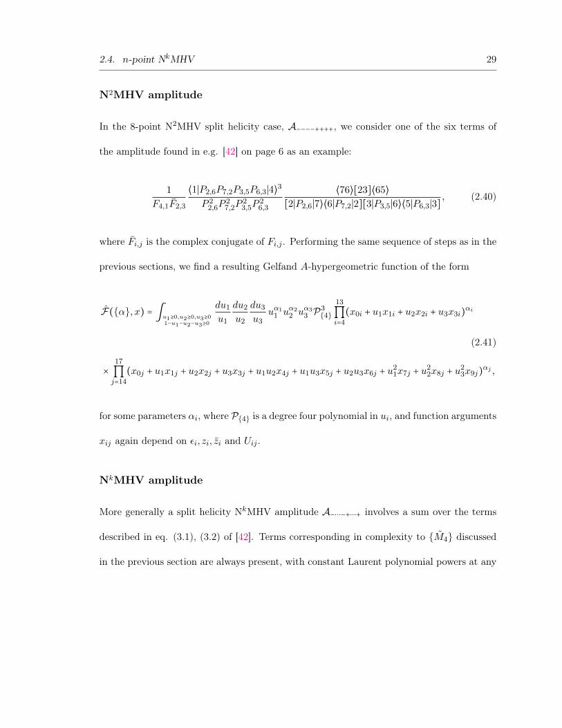
N2MHV amplitude
In the 8-point N2MHV split helicity case Aminusminusminusminus++++ we consider one of the six terms of
the amplitude found in eg [42] on page 6 as an example
1
F41F23
⟨1∣P26P72P35P63∣4⟩3
P 226P
272P
235P
263
⟨76⟩[23]⟨65⟩[2∣P26∣7⟩⟨6∣P72∣2][3∣P35∣6⟩⟨5∣P63∣3]
(240)
where Fij is the complex conjugate of Fij Performing the same sequence of steps as in the
previous sections we find a resulting Gelfand A-hypergeometric function of the form
F(α x) = intu1ge0u2ge0u3ge01minusu1minusu2minusu3ge0
du1
u1
du2
u2
du3
u3uα1
1 uα22 uα3
3 P34
13
prodi=4
(x0i + u1x1i + u2x2i + u3x3i)αi
(241)
times17
prodj=14
(x0j + u1x1j + u2x2j + u3x3j + u1u2x4j + u1u3x5j + u2u3x6j + u21x7j + u2
2x8j + u23x9j)αj
for some parameters αi where P4 is a degree four polynomial in ui and function arguments
xij again depend on εi zi zi and Uij
NkMHV amplitude
More generally a split helicity NkMHV amplitude Aminus⋯minus+⋯+ involves a sum over the terms
described in eq (31) (32) of [42] Terms corresponding in complexity to M4 discussed
in the previous section are always present with constant Laurent polynomial powers at any
30 Chapter 2 Tree-level Gluon Amplitudes on the Celestial Sphere
k However for higher k the most complicated contributing summands result in hypergeo-
metric integrals schematically given by
F(α x) =int u1unminus4ge01minusu2minus⋯minusunminus4ge0
nminus4
prodl=2
dululuαl
l
⎛⎝
1 minusnminus4
sumj=2
uj⎞⎠
α1
P32k (prod
i
(P i1)αi)
⎛⎝prodj
(Pj2)αj
⎞⎠
(242)
where αi are parameters and Pd is a degree d polynomial in ua Here we explicitly see an
increase in power of the Laurent polynomials with increasing k in NkMHV The examples
above feature the Gelfand A-hypergeometric function F The increase in Laurent polyno-
mial degree is traced back to the presence of Mandelstam invariants P 2ij for degree two
polynomials as well as the factors ⟨a∣PijPklPrt∣b⟩ for higher degree polynomials The
length of chains of the Pij depends on n and k such that multivariate Laurent polynomials
of any positive degree are present at sufficiently high n k
Similar generalized hypergeometric functions or equivalently generalized Euler integrals
are found in the case of string scattering amplitudes [43 44] It will be interesting to explore
this connection further
25 Generalized hypergeometric functions 31
25 Generalized hypergeometric functions
The Aomoto-Gelfand hypergeometric functions of type (n + 1m + 1) relevant in this work
can be defined as in section 351 of [38]
ϕ(α x) equivintu1ge0unge01minussuma uage0
m
prodj=0
Pj(u)αjdϕ (243)
dϕ =dPj1Pj1
and and dPjnPjn
0 le j1 lt lt jn lem (244)
Pj(u) =x0j + x1ju1 + + xnjun 1 le j lem (245)
where here the parameters αi collectively describe all the powers for the factors in the
integrand When all αi are zero the function reduces to the Aomoto polylogarithm
The arguments xij of the hypergeometric function of type (m+ 1 n+ 1) in (245) can be
arranged in a matrix
X =
⎛⎜⎜⎜⎜⎜⎜⎜⎜⎜⎜⎜⎜⎜⎝
x00 x0m
x10 x1m
⋮ ⋱ ⋮
xn0 xnm
⎞⎟⎟⎟⎟⎟⎟⎟⎟⎟⎟⎟⎟⎟⎠
(246)
Each column in this matrix defines a hyperplane in Cn that appears in the hypergeometric
integral as (x0j +sumni=1 xijui)αi Furthermore (n + 1) times (n + 1) minor determinants of the
matrix can be regarded as Pluumlcker coordinates on the Grassmannian Gr(n + 1m + 1) over
the space of arguments xij
32 Chapter 2 Tree-level Gluon Amplitudes on the Celestial Sphere
Sometimes it is convenient to transform the argument arrangement (246) to the following
gauge fixed form
⎛⎜⎜⎜⎜⎜⎜⎜⎜⎜⎜⎜⎜⎜⎝
1 0 0 1 1 1
0 1 0 minus1 minusx11 minusx1mminusnminus1
⋮ ⋱ minus1 ⋮ ⋮ ⋮
0 0 1 minus1 minusxn1 minusxnmminusnminus1
⎞⎟⎟⎟⎟⎟⎟⎟⎟⎟⎟⎟⎟⎟⎠
(247)
In this case the hypergeometric function can then be written in the following two equivalent
ways eq (324) of [38]
F ((αi) (βj) γx) =c1intu1ge0unge01minussuma uage0
dnun
prodi=1
uαiminus1i sdot (1 minus
n
suml=1
ul)γminussumi αiminus1mminusnminus1
prodj=1
(1 minusn
sumi=1
xijui)minusβj
c1 =Γ(γ)Γ(γ minusn
sumi=1
αi) sdotn
prodi=1
Γ(αi) (248)
and the dual representation in eq (325) of [38]
F ((αi) (βj) γx) =c2intu1ge0umminusnminus1ge01minussuma uage0
dmminusnminus1umminusnminus1
prodi=1
uβiminus1i sdot (1 minus
mminusnminus1
suml=1
ul)γminussumi βiminus1n
prodj=1
(1 minusmminusnminus1
sumi=1
xjiui)minusαj
c2 =Γ(γ)Γ(γ minusmminusnminus1
sumi=1
βi) sdotmminusnminus1
prodi=1
Γ(βi) (249)
where the parameters are assumed to satisfy the conditions
αi notin Z 1 le i le n βj notin Z 1 le j lem minus n minus 1
γ minusn
sumi=1
αi notin Z γ minusmminusnminus1
sumj=1
βj notin Z(250)
25 Generalized hypergeometric functions 33
The hypergeometric functions (243) comprise a basis of solutions to the defining set of
differential equations
(1)n
sumi=0
xijpartϕ
partxij= αjϕ 0 le j lem
(2)m
sumj=0
xijpartϕ
partxij= minus(1 + αi)ϕ 0 le i le n (251)
(3) part2ϕ
partxijpartxpq= part2ϕ
partxiqpartxpj 0 le i p le n 0 le j q lem
In cases where factors of the integrand are non-linear in the integration variables the
functions can be generalized further to Gelfand A-hypergeometric functions [45 46] defined
as
F(α x) = intu1ge0ukge01minussuma uage0
prodi
Pi(u1 uk)αiuα11 uαk
k du1duk (252)
where αi are complex parameters and Pi now are Laurent polynomials in u1 uk
35
Chapter 3
Celestial Amplitudes Conformal
Partial Waves and Soft Limits
This chapter is based on the publication [47]
Pasterski Shao and Strominger (PSS) have proposed a map between S-matrix elements
in four-dimensional Minkowski spacetime and correlation functions in two-dimensional con-
formal field theory (CFT) living on the celestial sphere [8 34] Celestial CFT is interesting
both for understanding the long elusive holographic description of flat spacetime [48] as well
as for exploring the mathematical structures of amplitudes In recent years many remarkable
properties of amplitudes have been uncovered via twistor space momentum twistor space
scattering equations etc(see [49] for review) hence it is quite plausible that exploring prop-
erties of celestial amplitudes may also lead to new insights
A key idea behind the PSS proposal was to transform the plane wave basis to a manifestly
conformally covariant basis called the conformal primary wavefunction basis This basis
was constructed explicitly by Pasterski and Shao [9] for particles of various spins in diverse
dimensions The celestial sphere is the null infinity of four-dimensional Minkowski spacetime
36 Chapter 3 Celestial Amplitudes Conformal Partial Waves and Soft Limits
The double cover of the four-dimensional Lorentz group is identified with the SL(2C)
conformal group of the celestial sphere Two-dimensional correlators on the celestial sphere
will be referred to as celestial amplitudes from here on
The celestial amplitudes of massless particles are given by Mellin transforms of the
corresponding four-dimensional amplitudes
An(zj zj) = intinfin
0
n
prodl=1
dωl ω∆lminus1l An(kl) (31)
where ∆l = 1 + iλl with λl isin R [9] are conformal dimensions taking values in the principal
continuous series in order to ensure the orthogonality and completeness of the conformal
primary wavefunction basis Further details are given below
In the spirit of recent developments in understanding scattering amplitudes from the on-
shell perspective by studying symmetries analytic properties and unitarity many recent
studies have delved into similar aspects of celestial amplitudes The structure of factorization
of singularities of celestial amplitudes was investigated in [33] three- and four-point gluon
amplitudes were computed in [34] and arbitrary tree-level ones in [31] Celestial four-point
string amplitudes have been discussed in [50] Unitarity via the manifestation of the optical
theorem on celestial amplitudes has been observed recently [36 35] and the generators of
Poincareacute and conformal groups in the celestial representation were constructed in [51]
This paper is organized as follows In section 31 we compute massless scalar four-point
celestial amplitudes and study its properties such as conformal partial wave decomposition
crossing relations and optical theorem In section 32 we derive conformal partial wave
decomposition for four-point gluon celestial amplitude and in section 33 single and double
31 Scalar Four-Point Amplitude 37
mk2
k1
k3
k4
k2
k1
k3
k4
m
k2
k1
k3
k4
m
Figure 31 Four-Point Exchange Diagrams
soft limits for all gluon celestial amplitudes The conformal partial wave decomposition
formalism is summarized in appendix 34 and details about inner product integrals required
in the main text are evaluated in appendix 35
Note added During this work we became aware of related work by Pate Raclariu and
Strominger [52] which has some overlap with section 4 of our paper
31 Scalar Four-Point Amplitude
In this section we study a tree level four-point amplitude of massless scalars mediated by
exchange of a massive scalar depicted on Figure 311
The corresponding celestial amplitude (31) is
A4(zj zj) = g2intinfin
0
4
prodj=1
dωj ω∆jminus1j δ(4) (
4
sumi=1
ki)( 1
(k1+k2)2+m2+ 1
(k1+k3)2+m2+ 1
(k1+k4)2+m2)
(32)
where zj zj are coordinates on the celestial sphere and ωj are the energies Defining εj = minus1
(+1) for incoming (outgoing) particles we can parameterize the momenta kmicroj as
kmicroj = εjωj (1 + ∣zj ∣2 zj + zj izj minus izj 1 minus ∣zj ∣2) (33)
1The same amplitude in three dimensions was studied in [35]
38 Chapter 3 Celestial Amplitudes Conformal Partial Waves and Soft Limits
Under conformal transformations by construction [9] the four-point celestial amplitude
behaves as a four-point CFT correlation function of operators with conformal weights
(hj hj) =1
2(∆j + Jj ∆j minus Jj) (34)
where Jj are spins We can split the four-point celestial amplitude into a conformally
invariant function of only the cross-ratios A4(z z) and a universal prefactor
A4(zj zj) =( z24
z14)h12 ( z14
z13)h34
zh1+h212 zh3+h4
34
( z24
z14)h12 ( z14
z13)h34
zh1+h212 zh3+h4
34
A4(z z) (35)
where we define hij = hi minus hj hij = hi minus hj and cross-ratios
z = z12z34
z13z24 z = z12z34
z13z24with zij = zi minus zj zij = zi minus zj (36)
Letrsquos fix the external points in (32) as z1 = 0 z2 = z z3 = 1 z4 = 1τ with τ rarr 0 and
compute
A4(z) equiv ∣z∣∆1+∆2 limτrarr0
τminus2∆4A4(0 z11τ) (37)
We will consider the case where particles 1 and 2 are incoming while 3 and 4 are outgoing
so ε1 = ε2 = minusε3 = minusε4 = minus1 and denote it as 12harr 34 The s-channel diagram on figure 31 is
A12harr344s (z) sim g2∣z∣∆1+∆2 lim
τrarr0τminus2∆4 int
infin
0
4
prodi=1
dωi ω∆iminus1i δ(4)
⎛⎝
4
sumj=1
kj⎞⎠
1
m2 minus 4ω1ω2∣z∣2 (38)
31 Scalar Four-Point Amplitude 39
The momentum conservation delta functions can be rewritten as
δ(4)⎛⎝
4
sumj=1
kj⎞⎠= 4τ2
ω1δ(iz minus iz)
4
prodi=2
δ(ωi minus ωlowasti ) (39)
where
ωlowast2 = ω1
z minus 1 ωlowast3 = zω1
z minus 1 ωlowast4 = zω1τ
2 (310)
The delta function only has solutions when all the ωlowasti are positive so z gt 1
Then (38) reduces to a single integral
A12harr344s (z) sim g2δ(iz minus iz)z∆1+∆2 lim
τrarr0τ2minus2∆4 int
infin
0dω1ω
∆1minus21
4
prodi=2
(ωlowasti )∆iminus1 1
m2 minus 4z2
zminus1ω21
= g2 (im2)2αminus2
sin(πα) δ(iz minus iz) z2 (z minus 1)h12minush34 (311)
Adding the s- t- and u-channel contributions we obtain our final result
A12harr344 (z) sim g2 (m2)2αminus2
sin(πα) δ(iz minus iz) z2 (z minus 1)h12minush34 (eπiα + ( z
z minus 1)α
+ zα) (312)
where
α =4
sumi=1
hi minus 2 (313)
Let us discuss some properties of this expression
40 Chapter 3 Celestial Amplitudes Conformal Partial Waves and Soft Limits
First it is straightforward to verify that the Poincareacute generators on the celestial sphere
constructed in [51]
L1i = (1 minus z2i )partzi minus 2zihi
L1i = (1 minus z2i )partzi minus 2zihi
P0i = (1 + ∣zi∣2)e(parthi+parthi)2
P2i = minusi(zi minus zi)e(parthi+parthi)2
L2i = (1 + z2i )partzi + 2zihi L3i = 2(zipartzi + hi)
L2i = (1 + z2i )partzi + 2zihi L3i = 2(zipartzi + hi)
P1i = (zi + zi)e(parthi+parthi)2
P3i = (1 minus ∣zi∣2)e(parthi+parthi)2
(314)
annihilate the celestial amplitude on the support of the delta function δ(iz minus iz)
Second we can show that A4 satisfies the crossing relations
A13harr244 (1 minus z) = (1 minus z
z)
2(h2+h3)A13harr24
4 (z) 0 lt z lt 1 (315)
as well as
A13harr244 (z) = z2(h1+h4)A12harr34
4 (1z)
= (1 minus z)2(h12minush34)A14harr234 ( z
z minus 1) 0 lt z lt 1 (316)
The relations (315) and (316) generalize similar relations in [35]
Third the conformal partial wave decomposition of s-channel celestial amplitude
(311)2 is computed in the appendix 34 35 and takes the following form
A12harr344s (z) sim g
2 (im2)2αminus2
2 sin(πα) intC
d∆
4π2
Γ (1minus∆2 minush12)Γ (∆
2 minush12)Γ (1minus∆2 minush34)Γ (∆
2 minush34)Γ(1 minus∆)Γ(∆ minus 1) Ψ∆
hi(z z)
(317)
2The other two channels can be obtained in similar manner
31 Scalar Four-Point Amplitude 41
where Ψ∆hi(z z) is given in (345) restricted to the internal scalar case with J = 0 and the
contour C runs from 1 minus iinfin to 1 + iinfin
The gamma functions in (317) unambiguously specify all pole sequences in conformal
dimensions Closing the contour to the right or left of the complex axis in ∆ we find simple
poles at ∆ and their shadows at ∆ given by
∆
2= 1 minus h12 + n
∆
2= 1 minus h34 + n
∆
2= h12 minus n
∆
2= h34 minus n (318)
with n = 0123
Finally letrsquos explicitly check the celestial optical theorem derived by Shao and Lam in
[35] which relates the imaginary part of the four-point celestial amplitude to the product
of two three-point celestial amplitudes with the appropriate integration measure Taking
imaginary part of (317) we obtain
Im [A12harr344s (z)] sim int
Cd∆micro(∆)C(h1 h2 ∆)C(h3 h4 2 minus∆)Ψ∆
hi(z z) (319)
up to some overall constants independent of hi Here C(hi hj ∆) is the coefficient of the
three-point function given by [35]
C(hi hj ∆) = g (m2)hi+hjminus2
4hi+hj
Γ (hij + ∆2)Γ (∆
2 minus hij)Γ(∆) (320)
micro(∆) is the integration measure
micro(∆) = Γ(∆)Γ(2 minus∆)4π3Γ(∆ minus 1)Γ(1 minus∆) (321)
42 Chapter 3 Celestial Amplitudes Conformal Partial Waves and Soft Limits
and Ψ∆hi(z z) is
Ψ∆hi(z z) equiv
Γ (1 minus ∆2 minus h12)Γ (∆
2 minus h34)Γ (∆
2 + h12)Γ (1 minus ∆2 + h34)
Ψ∆hi(z z) (322)
32 Gluon Four-Point Amplitude
In this section we study the massless four-point gluon celestial amplitude which has been
computed in [34] and is given by
A12harr34minusminus++ (z) sim δ(iz minus iz)∣z∣3∣1 minus z∣h12minush34minus1 z gt 1 (323)
where the conformal ratios z z are defined in (36)
Evaluating the integral in appendix 35 we find the conformal partial wave expansion is
given by the following simple result3
A12harr34minusminus++ (z) sim 2i
infinsumJ=0
prime
intC
dh
4π2Ψhh
hihi
π (1 minus 2h)(2h minus 1 minus 2J)(h34minush12) sin(π(h12minush34))
(Γ(hminush12)Γ(1+Jminush34minush)Γ(h+h12)Γ(1+J+h34minush)
+(h12 harr h34))
(324)
where sumprime means that the J = 0 term contributes with weight 12
There is no truncation of the spins J in this case so primary operators of all integer
spins contribute to the OPE expansion of the external gluon operators in contrast with the
previously considered scalar case3When considering J lt 0 take hharr h in the expansion coefficient
33 Soft limits 43
Poles ∆ and shadow poles ∆ are located at
∆ minus J2
= 1 minus h12 + n ∆ minus J
2= 1 minus h34 + n
∆ + J2
= h12 minus n ∆ + J
2= h34 minus n
(325)
with n = 0123 These poles are integer spaced as expected
33 Soft limits
Single soft limits
In this section we study the analog of soft limits for celestial amplitudes The universal
soft behavior of color-ordered gluon scattering amplitudes corresponding to ωk rarr 0 is
well-known [53] and takes the form
limωkrarr0
A`k=+1n = ⟨k minus 1k + 1⟩
⟨k minus 1k⟩⟨k k + 1⟩Anminus1
limωkrarr0
A`k=minus1n = [k minus 1k + 1]
[k minus 1k][k k + 1]Anminus1
(326)
where `k is the helicity of particle k
The spinor-helicity variables are related to the celestial sphere variables via [34]
[ij] = 2radicωiωj zij ⟨ij⟩ = minus2εiεj
radicωiωjzij (327)
44 Chapter 3 Celestial Amplitudes Conformal Partial Waves and Soft Limits
Conformal primary wavefunctions become soft (pure gauge) when ∆k rarr 1 (or λk rarr 0) [9 54]
In this limit we can utilize the delta function representation4
δ(x) = 1
2limλrarr0
iλ ∣x∣iλminus1 (328)
such that (31) becomes
limλkrarr0
An(zj zj) =1
iλk
n
prodj=1jnek
intinfin
0dωj ω
iλjj int
infin
0dωk 2 δ(ωk)ωkAn(ωj zj zj) (329)
We see that the λk rarr 0 limit localizes the integral at ωk = 0 and we obtain
limλkrarr0
AJk=+1n = 1
iλk
zkminus1k+1
zkminus1kzk k+1Anminus1 (330)
limλkrarr0
AJk=minus1n = 1
iλk
zkminus1k+1
zkminus1kzk k+1Anminus1 (331)
An alternative derivation of these relations was given in [55]
Double soft limits
For consecutive soft limits one can apply (330) or (331) multiple times and the con-
secutive soft factors are simply products of single soft factors4See httpmathworldwolframcomDeltaFunctionhtml
33 Soft limits 45
For simultaneous double soft limits energies of particles are simultaneously scaled by δ
so ωk rarr δωk and ωl rarr δωl with δ rarr 0 which for example yields [56 57]
limδrarr0An(δω1 δω2 ωj zk zk) =
1
⟨n∣1 + 2∣3] ( [13]3⟨n3⟩[12][23]s123
+ ⟨n2⟩3[n3]⟨n1⟩⟨12⟩sn12
)Anminus2(ωj zj zj)
(332)
for `1 = +1 `2 = minus1 j = 3 n and k = 1 n Here sijl = (ki + kj + kl)2 More generally
we will write
limδrarr0An(δωk δωl ωj zi zi) = DS(k`k l`l)Anminus2(ωj zj zj) (333)
where DS(k`k l`l) is the simultaneous double soft factor
For celestial amplitudes the analog of the simultaneous double soft limit is to take two
λrsquos scale them by ε λk rarr ελk and λl rarr ελl and take the ε rarr 0 limit To implement this
practically in (31) we change variables for the associated ωrsquos
ωk = r cos(θ) ωl = r sin(θ) 0 le r ltinfin 0 le θ le π2 (334)
The mapping (31) becomes
An(zj zj) =n
prodj=1jnekl
intinfin
0dωj ω
iλjj int
infin
0dr int
π2
0dθ r(iλk+iλl)εminus1
times (cos(θ))iλkε(sin(θ))iλlεr2An(ωj zj zj)
(335)
46 Chapter 3 Celestial Amplitudes Conformal Partial Waves and Soft Limits
We can use (328) to obtain a delta function in r which enforces the simultaneous double
soft limit for the scattering amplitude as in (332) The result is
limεrarr0An(λkε λlε) = DS(kJk lJl)Anminus2 (336)
where DS(kJk lJl) is the simultaneous double soft factor on the celestial sphere
DS(kJk lJl) = 1
(iλk + iλl)ε[2int
π2
0dθ (cos(θ))iλkε(sin(θ))iλlε [r2DS(k`k l`l)]
r=0]εrarr0
(337)
As an example consider the simultaneous double soft factor in (332) We can use (327) to
translate it into celestial sphere coordinates and plug into (337) to obtain
DS(1+12minus1) sim 1
2(iλ1 + iλ2)ε21
zn1z23( 1
iλ1
zn3z2n
z12z2n+ 1
iλ2
z3nz31
z12z31) (338)
Explicitly let us check (336) by considering the six-point NMHV split helicity amplitude
[42]
A+++minusminusminus = δ(4) (6
sumi=1
ki)1
4ω1⋯ω6
times⎡⎢⎢⎢⎢⎢⎣
ω21ω
24(ω3z34z13minusω2z24z12)3
(ω3ω4z34z34minusω2ω4z24z24minusω2ω3z23z23)
z23z34z56z61 (ω4z24z54 minus ω3z23z35)+
ω23ω
26(ω4z46z34+ω5z56z35)3
(ω3ω4z34z34+ω3ω5z35z35+ω4ω5z45z45)
z12z16z34z45 (ω3z23z35 + ω4z24z45)
⎤⎥⎥⎥⎥⎥⎦
(339)
34 Conformal Partial Wave Decomposition 47
and map it via (31) Taking the simultaneous double soft limit of particles 3 and 4 as
prescribed in (336) we find
limεrarr0A+++minusminusminus(λ3ε λ4ε) =
1
2(iλ3 + iλ4)ε21
z23z45( 1
iλ3
z25z41
z34z42+ 1
iλ4
z52z53
z34z53) A++minusminus (340)
where the four-point correlator is given by mapping the appropriate MHV amplitude via
(31)
A++minusminus = 4iδ(λ1 + λ2 + λ5 + λ6)z3
56 δ(izprime minus izprime)z12z2
25z216z25z61
(z15z61
z25z26)iλ2minus1
(z12z16
z25z56)iλ5+1
(z15z12
z56z26)iλ6+1
(341)
where zprime = z12z56
z25z61and zprime = z12z56
z25z61 The conformal soft factor found in (340) matches our
general result by taking the double soft factor [56 57]
1
⟨2∣3 + 4∣5] ( [35]3⟨25⟩[34][45]s345
+ ⟨24⟩3[25]⟨23⟩⟨34⟩s234
) (342)
and mapping it via (337)
It is straightforward to generalize (336) to m particles taken simultaneously soft by
introducing m-dimensional spherical coordinates as in (334) and scale m λrsquos by ε
34 Conformal Partial Wave Decomposition
In the CFT four-point function defined as (35) we can expand the conformally invariant
part A4(z z) on the basis of conformal partial waves Ψhh
hihi(z z) As can be shown along
48 Chapter 3 Celestial Amplitudes Conformal Partial Waves and Soft Limits
the lines of [58 60 59] the expansion takes the following form
A4(z z) = iinfinsumJ=0
prime
intCd∆ Ψhh
hihi(z z)(1 minus 2h)(2h minus 1)
(2π)2⟨A4(z z)Ψhh
hihi(z z)⟩ (343)
where h minus h = J h + h = ∆ = 1 + iλ The contour C runs from 1 minus iinfin to 1 + iinfin The
integration and summation is over all dimensions and spins of exchanged primary operators
in the theory sumprime means that the J = 0 summand contributes with a weight of 12 The
inner product is defined by
⟨G(z z) F (z z)⟩ equiv intdzdz
(zz)2G(z z)F (z z) (344)
The conformal partial waves Ψhh
hihi(z z) have been computed in [61 62 63] and are
given by
Ψhh
hihi(z z) =cprime1F+(z z) + cprime2Fminus(z z) (345)
with
F+(z z) =1
zh34 zh342F1 (
1 minus h + h34 h + h34
1 + h12 + h341
z) 2F1 (
1 minus h + h34 h + h34
1 + h12 + h341
z) (346)
Fminus(z z) =zh12 zh122F1 (
1 minus h minus h12 h minus h12
1 minus h12 minus h341
z) 2F1 (
1 minus h minus h12 h minus h12
1 minus h12 minus h341
z)
cprime1 =(minus1)hminush+h12minush12Γ (minush12 minus h34)
Γ (1 + h12 + h34)Γ (1 minus h + h12)Γ (h + h34)Γ (h + h12)Γ (1 minus h + h34)Γ (1 minus h minus h12)Γ (h minus h34)Γ (h minus h12)Γ (1 minus h minus h34)
cprime2 =(minus1)hminush+h34minush34Γ (h12 + h34)
Γ (1 minus h12 minus h34)
35 Inner Product Integral 49
Here we made use of hypergeometric identities discussed in [62] to rewrite the result in a
form which is suited for the region z z gt 1
Conformal partial waves are orthogonal with respect to the inner product (344)
⟨Ψhh
hihi(z z)Ψhprimehprime
hihi(z z)⟩ = (2π)2
(1 minus 2h)(2h minus 1)δJJ primeδ(λ minus λprime) (347)
The basis functions (345) span a complete basis for bosonic fields on each of the ranges
(J isin Z λ isin R+ ∣ J isin Z+ λ isin R ∣ J isin Z λ isin Rminus ∣ J isin Zminus λ isin R) (348)
We can perform the ∆ integration in (343) by collecting residues of poles located to the
left or to the right of the complex axis One can use eg the integral representation of the
conformal partial wave (345) (given by eq (7) in [63]) to make sure that the half-circle
integration at infinity vanishes
35 Inner Product Integral
In this appendix we evaluate the inner product
⟨A4(z z)Ψhh
hihi(z z)⟩ equiv int
dzdz
(zz)2δ(iz minus iz) ∣z∣2+σ ∣z minus 1∣h12minush34minusσ Ψhh
hihi(z z) (349)
for σ = 0 and σ = 1 where Ψhh
hihi(z z) is given by (345)5
5Note that in both of our examples we have hij = hij and the complex conjugation prescription hrarr 1minus hhrarr 1 minus h hij rarr minushij and zharr z
50 Chapter 3 Celestial Amplitudes Conformal Partial Waves and Soft Limits
First we change integration variables to z = x + iy z = x minus iy and localize the delta
function on y = 0 Subsequently we write the hypergeometric functions from (345) in the
following Mellin-Barnes representation
2F1(a b c z) =Γ(c)
Γ(a)Γ(b)Γ(c minus a)Γ(c minus b) intCds
2πi(1 minus z)sΓ(minuss)Γ(c minus a minus b minus s)Γ(a + s)Γ(b + s)
(350)
where (1 minus z) isin CRminus and the contour C goes from minus to plus complex infinity while
separating pole sequences in Γ(minuss)Γ(c minus a minus b minus s) from pole sequences in Γ(a + s)Γ(b + s)
The x gt 1 integral then gives a beta function which we express in terms of gamma
functions At this point similarly to section 34 in [64] the gamma function arguments in
the integrand arrange themselves exactly such that one of the Mellin-Barnes integrals (350)
can be evaluated by second Barnes lemma6 The final inverse Mellin transform integral is
then done by closing the integration contour to the left or to the right of the complex axis
Performing the sum over all residues of poles wrapped by the contour in this process we
obtain
⟨A4(z z)Ψhh
hihi(z z)⟩ = π2(minus1)hminush csc (π (h12 minus h34)) csc (π (h12 + h34))Γ(1 minus σ) (351)
⎡⎢⎢⎢⎢⎢⎣
⎛⎜⎝
Γ (1 minus σ + h12 minus h34) 4F3 ( 1minusσ1minush+h12h+h121minusσ+h12minush34
2minushminusσ+h12hminusσ+h12+1h12minush34+1 1)Γ (h12 minus h34 + 1)Γ (1 minus h + h34)Γ (h + h34)Γ (2 minus h minus σ + h12)Γ (h minus σ + h12 + 1)
minus (h12 harr h34)⎞⎟⎠
+( Γ(1minushminush12)Γ(hminush12)Γ(1minusσminush12+h34)
Γ(1minush12+h34)Γ(2minushminusσminush12)Γ(hminusσminush12+1) 4F3 ( 1minusσ1minushminush12hminush121minusσminush12+h34
2minushminusσminush12hminusσminush12+11minush12+h34 1) minus (h12 harr h34))
Γ (1 minus h + h12)Γ (h + h12)Γ (1 minus h + h34)Γ (h + h34)
⎤⎥⎥⎥⎥⎥⎥⎦
6We assume the integrals to be regulated appropriately such that these formal manipulations hold
35 Inner Product Integral 51
where we used identities such as sin(x+ πh) sin(y + πh) = sin(x+ πh) sin(y + πh) for integer
J and sin(πx) = π(Γ(x)Γ(1 minus x)) to write (351) in a shorter form
Evaluation for σ = 0
When σ = 0 one upper and one lower parameter in the 4F3 hypergeometric functions
become equal and cancel so that the functions reduce to 3F2 Interestingly an even greater
simplification occurs as
3F2 (1 a minus c + 1 a + ca minus b + 2 a + b + 1
1) =Γ(aminusb+2)Γ(a+b+1)Γ(aminusc+1)Γ(a+c) minus (a minus b + 1)(a + b)
(b minus c)(b + c minus 1) (352)
Then making use of various sine- and gamma function identities as mentioned above it
turns out that the result is proportional to
sin(2πJ)2πJ
= 1 J = 0
0 J ne 0 (353)
Therefore the only non-vanishing inner product in this case comes from the scalar conformal
partial wave Ψ∆hiequiv Ψhh
hihi∣J=0
which simplifies to
⟨A4(z z)Ψ∆hi(z z)⟩ =
Γ (1 minus ∆2 minus h12)Γ (∆
2 minus h12)Γ (1 minus ∆2 minus h34)Γ (∆
2 minus h34)Γ(2 minus∆)Γ(∆) (354)
Evaluation for σ = 1
As we take σ rarr 1 the overall factor Γ(1 minus σ) diverges However the rest of the terms
conspire to cancel this pole so that the limit σ rarr 1 is finite The simplification of the result
in all generality is quite tedious here we instead discuss a less rigorous but quick way to
52 Chapter 3 Celestial Amplitudes Conformal Partial Waves and Soft Limits
arrive at the end result
The cases for the first few values of J = 01 can be simplified directly eg in Mathe-
matica We recognize that the result is always proportional to csc(π(h12minush34))(h12minush34)
To quickly arrive at the full result start with (351) and divide out the overall factor
csc(π(h12 minus h34))(h12 minus h34) By the previous observation we see that the rest is finite
in h12 minus h34 rarr 0 Sending h34 rarr h12 under a small 1 minus σ deformation the hypergeometric
functions become equal to 1 for σ rarr 1 and the remaining terms simplify To recover the full
h12 h34 dependence it then suffices to match these terms eg to the specific example in the
case J = 1 which then for all J ge 0 leads to
⟨A4(z z)Ψhh
hihi(z z)⟩ = π csc(π(h12 minus h34))
(h34 minus h12)(Γ(h minus h12)Γ(1 minus h34 minus h)
Γ(h + h12)Γ(1 + h34 minus h)+ (h12 harr h34))
(355)
To obtain the result for J lt 0 substitute hharr h
53
Chapter 4
Yangian Invariants and Cluster
Adjacency in N = 4 Yang-Mills
This chapter is based on the publication [65]
In recent years cluster algebras have shed interesting light on the mathematical properties
of scattering amplitudes in planar N = 4 supersymmetric Yang-Mills (SYM) theory [5]
Cluster algebraic structure manifests itself in several distinct ways notably including the
appearance of certain Gr(4 n) cluster coordinates in the symbol alphabets [5 66 67 68]
cobrackets [5 69 70 71 72] and integrands [30] of n-particle amplitudes
There has been a recent revival of interest in the cluster structure of SYM amplitudes
following the observation [73] that certain amplitudes exhibit a property called cluster adja-
cency Cluster coordinates are grouped into sets called clusters with two coordinates being
called adjacent if there exists a cluster containing both The central problem of the ldquocluster
adjacencyrdquo literature is to identify (and hopefully to explain) correlations between sets of
pairs (or larger groupings) of cluster coordinates and the manner in which those pairs are
observed to appear together in various amplitudes
54 Chapter 4 Yangian Invariants and Cluster Adjacency in N = 4 Yang-Mills
For example for loop amplitudes all evidence available to date [81 22 131 75 76
77 78 80 79 82 89 83] supports the hypothesis that two cluster coordinates appear in
adjacent symbol entries only if they are cluster adjacent In [89] it was shown that this
type of cluster adjacency implies the Steinmann relations [84 85 86] For tree amplitudes a
somewhat analogous version of cluster adjacency was proposed in [81] where it was checked
in several cases and conjectured in general that every Yangian invariant in the BCFW
expansion of tree-level amplitudes in SYM theory has poles given by cluster coordinates
that are all contained in a common cluster
In this paper we provide further evidence for this and the even stronger conjecture that
cluster adjacency holds for every rational Yangian invariant in SYM theory even those that
do not appear in any representation of tree amplitudes
In Sec 2 we review the main tool of our analysis the Sklyanin Poisson bracket [87 88]
which can be used to diagnose whether two cluster coordinates on Gr(4 n) are adjacent
which we will call the bracket test [89] In Sec 3 we review the Yangian invariants of
SYM theory and explain how (in principle) to use the bracket test to provide evidence that
NkMHV Yangian invariants satisfy cluster adjacency We carry out this check for all k le 2
invariants and many k = 3 invariants
Before proceeding we make a few comments clarifying the ways in which our tests are
weaker than the analysis of [81] and the ways in which they are stronger
1 It could have happened that only certain repreresentations of tree-level amplitudes
(depending perhaps on the choice of shifts during intermediate steps of BCFW re-
cursion) satisfy cluster adjacency but as already noted our results suggest that every
Chapter 4 Yangian Invariants and Cluster Adjacency in N = 4 Yang-Mills 55
rational Yangian invariant satisfies cluster adjacency If true this suggests that the
connection between cluster adjacency and Yangian invariants admits a mathematical
explanation independent of the physics of scattering amplitudes
2 For any fixed k there are finitely many functionally independent NkMHV Yangian
invariants If it is known that these all satisfy cluster adjacency it immediately follows
that the n-particle NkMHV amplitude satisfies cluster adjacency for all n Our results
therefore extend the analysis of [81] in both k and n
3 However unlike in [81] we make no attempt to check whether each of the polynomial
factors we encounter is actually a Gr(4 n) cluster coordinate Indeed for n gt 7 there
is no known algorithm for determining in finite time whether or not a given homoge-
neous polynomial in Pluumlcker coordinates is a cluster coordinate The bracket does not
help here it is trivial to write down pairs of polynomials that pass the bracket test
but are not cluster coordinates
4 In the examples checked in [81] it was noted that each term in a BCFW expansion of an
amplitude had the property that there exists a cluster of Gr(4 n) that simultaneously
contains all of the cluster coordinates appearing in the denominator of that term
Our test is much weaker in that it can only establish pairwise cluster adjacency For
example if we encounter a term with three polynomial factors p1 p2 and p3 our test
provides evidence that there is some cluster containing p1 and p2 and also some cluster
containing p2 and p3 and also some cluster containing p1 and p3 but the bracket
cannot provide any evidence for or against the existence of a cluster simultaneously
containing all three
56 Chapter 4 Yangian Invariants and Cluster Adjacency in N = 4 Yang-Mills
41 Cluster Coordinates and the Sklyanin Poisson Bracket
The objects of study in this paper will be certain rational functions on the kinematic space of
n cyclically ordered massless particles of the type that appear in tree-level gluon scattering
amplitudes A point in this kinematic space is conveniently parameterized by a collection
of n momentum twistors [4] ZI1 ZIn each of which can be regarded as a four-component
(I isin 1 4) homogeneous coordinate on P3
In these variables dual conformal symmetry [3] is realized by SL(4C) transformations
For a given collection of nmomentum twistors the (n4) Pluumlcker coordinates are the SL(4C)-
invariant quantities
⟨i j k l⟩ equiv εIJKLZIi ZJj ZKk ZLl (41)
The Gr(4 n) Grassmannian cluster algebra whose structure has been found to underlie
at least certain amplitudes in SYM theory is a commutative algebra with generators called
cluster coordinates Every cluster coordinate is a polynomial in Pluumlckers that is homogeneous
under a projective rescaling of each momentum twistor separately for example
⟨1 2 6 7⟩⟨2 3 4 5⟩ minus ⟨1 2 4 5⟩⟨2 3 6 7⟩ (42)
Every Pluumlcker coordinate is on its own a cluster coordinate For n lt 8 the number of cluster
coordinates is finite and they can easily be enumerated but for n gt 7 the number of cluster
coordinates is infinite
The cluster coordinates of Gr(4 n) are grouped into non-disjoint sets of cardinality 4nminus15
41 Cluster Coordinates and the Sklyanin Poisson Bracket 57
called clusters Two cluster coordinates are said to be cluster adjacent if there exists a cluster
containing both The n Pluumlcker coordinates ⟨1 2 3 4⟩ ⟨2 3 4 5⟩ ⋯ ⟨n1 2 3⟩ containing four
cyclically adjacent momentum twistors play a special role these are called frozen coordinates
and are elements of every cluster Therefore each frozen coordinate is adjacent to every
cluster coordinate
Two Pluumlcker coordinates are cluster adjacent if and only if they satisfy the so-called weak
separation criterion [90] In order to address the central problem posed in the Introduction
it is desirable to have an efficient algorithm for testing whether two more general cluster
coordinates are cluster adjacent As proposed in [89] the Sklyanin Poisson bracket [87 88]
can serve because of the expectation (not yet completely proven as far as we are aware)
that two cluster coordinates a1 a2 are adjacent if and only if log a1 log a2 isin 12Z
In the next section we use the Sklyanin Poisson bracket to test the cluster adjacency prop-
erties of Yangian invariants To that end let us briefly review following [89] (see also [91])
how it can be computed First any generic 4 times n momentum twistor matrix ZIi can be
brought into the gauge-fixed form
ZIi =
⎛⎜⎜⎜⎜⎜⎜⎜⎜⎜⎜⎜⎜⎜⎝
1 0 0 0 y15 ⋯ y1
n
0 1 0 0 y25 ⋯ y2
n
0 0 1 0 y35 ⋯ y3
n
0 0 0 1 y45 ⋯ y4
n
⎞⎟⎟⎟⎟⎟⎟⎟⎟⎟⎟⎟⎟⎟⎠
(43)
58 Chapter 4 Yangian Invariants and Cluster Adjacency in N = 4 Yang-Mills
by a suitable GL(4C) transformation The Sklyanin Poisson bracket of the yrsquos is defined
as
yIa yJ b =1
2(sign(J minus I) minus sign(b minus a))yJayI b (44)
Finally the Sklyanin Poisson bracket of two arbitrary functions f g of momentum twistors
can be computed by plugging in the parameterization (43) and then using the chain rule
f(y) g(y) =n
sumab=1
4
sumIJ=1
partf
partyIa
partg
partyJ byIa yJ b (45)
42 An Adjacency Test for Yangian Invariants
The conformal [92] and dual conformal symmetry of scattering amplitudes in SYM theory
combine to generate a Yangian [11] symmetry Yangian invariants [3 93 94 96 95 28 98
30 97] are the basic building blocks in terms of which amplitudes can be constructed We
say that a Yangian invariant is rational if it is a rational function of momentum twistors
equivalently it has intersection number Γ = 1 in the terminology of [30 99] Any n-particle
tree-level amplitude in SYM theory can be written as the n-particle Parke-Taylor-Nair su-
peramplitude [2 100] times a linear combination of rational Yangian invariants (see for
example [101]) In general the linear combination is not unique since Yangian invariants
satisfy numerous linear relations
Yangian invariants are actually superfunctions an n-particle invariant is a polynomial
of uniform degree 4k in 4kn Grassmann variables χAi where k is the NkMHV degree For a
rational Yangian invariant Y the coefficient of each distinct term in its expansion in χrsquos can
42 An Adjacency Test for Yangian Invariants 59
be uniquely factored into a ratio of products of polynomials in Pluumlcker coordinates with
each polynomial having uniform weight in each momentum twistor separately Let pi
denote the union of all such polynomials that appear in the denominator of the expansion
of Y Then we say that Y passes the bracket test if
Ωij equiv log pi log pj isin1
2Z foralli j (46)
As explained in [30] n-particle Yangian invariants can be classified in terms of permuta-
tions on n elements Since the bracket test is invariant1 under the Zn cyclic group that shifts
the momentum twistors Zi rarr Zi+1 modn we only need to consider one member from each
cyclic equivalence class The number of cyclic classes of rational NkMHV Yangian invariants
with nontrivial dependence on n momentum twistors was tabulated for various k and n in
Table 3 of [30] We record these numbers here correcting typos in the (315) and (420)
entries
k
n5 6 7 8 9 10 11 12 13 14 15 16 17 18 19 20 Total
1 1 0 0 0 0 0 0 0 0 0 0 0 0 0 0 0 1
2 0 1 2 5 4 1 0 0 0 0 0 0 0 0 0 0 13
3 0 0 1 6 54 177 298 274 134 30 3 0 0 0 0 0 977
4 0 0 0 1 13 263 1988 7862 18532 28204 28377 18925 8034 2047 270 17 114533
When they appear in scattering amplitudes Yangian invariants typically have triv-
ial dependence on several of the particles For example the five-particle NMHV Yan-
gian invariant Y (1)(Z1 Z2 Z3 Z4 Z5) could appear in a nine-particle NMHV amplitude
as Y (1)(Z2 Z4 Z5 Z7 Z8) among other possibilities Fortunately because of the simple1Certainly the value of the Sklyanin Poisson bracket is not in general cyclic invariant since evaluating it
requires making a gauge choice which breaks cyclic symmetry such as in (43) but the binary statement ofwhether some pair does or does not have half-integer valued bracket is cyclic invariant
60 Chapter 4 Yangian Invariants and Cluster Adjacency in N = 4 Yang-Mills
sign(b minus a) dependence on column number in the definition (44) the bracket test is insen-
sitive to trivial dependence on additional momentum twistors2
Therefore for any fixed k but arbitrary n we can provide evidence for the cluster
adjacency of every rational n-particle NkMHV Yangian invariant by applying the bracket
test described above (46) to each one of the (finitely many) rational Yangian invariants In
the next few subsections we present the results of our analysis beginning with the trivial
but illustrative case of k = 1
421 NMHV
The unique k = 1 Yangian invariant is the well-known five-bracket [93] (originally presented
as an ldquoR-invariantrdquo in [3])
Y (1) = [12345] equiv δ(4)(⟨1 2 3 4⟩χA5 + cyclic)⟨1 2 3 4⟩⟨2 3 4 5⟩⟨3 4 5 1⟩⟨4 5 1 2⟩⟨5 1 2 3⟩ (47)
whose denominator contains the five factors
p1 p5 = ⟨1 2 3 4⟩ ⟨2 3 4 5⟩ ⟨3 4 5 1⟩ ⟨4 5 1 2⟩ ⟨5 1 2 3⟩ (48)
each of which is simply a Pluumlcker coordinate Evaluating these in the gauge (43) gives
p1 p5 = 1minusy15minusy2
5minusy35minusy4
5 (49)
2As in footnote 1 the actual value of the Sklyanin Poisson bracket will in general change if the particlerelabeling affects any of the first four gauge-fixed columns of Z
42 An Adjacency Test for Yangian Invariants 61
and evaluating the bracket (46) in this basis using (44) gives
Ω(1)ij = log pi log pj =
⎛⎜⎜⎜⎜⎜⎜⎜⎜⎜⎜⎜⎜⎜⎜⎜⎜⎜⎜⎝
0 0 0 0 0
0 0 12
12
12
0 minus12 0 1
212
0 minus12 minus1
2 0 12
0 minus12 minus1
2 minus12 0
⎞⎟⎟⎟⎟⎟⎟⎟⎟⎟⎟⎟⎟⎟⎟⎟⎟⎟⎟⎠
(410)
Since each entry is half-integer the five-bracket (47) passes the bracket test
We wrote out the steps in detail in order to illustrate the general procedure although
in this trivial case the conclusion was foregone for n = 5 each Pluumlcker coordinate in (47)
is frozen so each is automatically cluster adjacent to each of the others It is however
interesting to note that if we uplift (47) by introducing trivial dependence on additional
particles this simple argument no longer applies For example [13579] still passes the
bracket test even though it does not involve any frozen coordinates The fact that the five-
bracket [i j k lm] passes the bracket test for any choice of indices can be understood in
terms of the weak separation criterion [90] for determining when two Pluumlcker coordinates
are cluster adjacent The connection between the weak separation criterion and all Yangian
invariants with n = 5k will be explored in [102]
62 Chapter 4 Yangian Invariants and Cluster Adjacency in N = 4 Yang-Mills
422 N2MHV
The 13 rational Yangian invariants with k = 2 are listed in Table 1 of [30] (we disregard the
ninth entry in the table which is algebraic but not rational3) They are given by
Y(2)
1 = [12 (23) cap (456) (234) cap (56)6][23456]
Y(2)
2 = [12 (34) cap (567) (345) cap (67)7][34567]
Y(2)
3 = [123 (345) cap (67)7][34567]
Y(2)
4 = [123 (456) cap (78)8][45678]
Y(2)
5 = [12348][45678]
Y(2)
6 = [123 (45) cap (678)8][45678]
Y(2)
7 = [123 (45) cap (678) (456) cap (78)][45678] (411)
Y(2)
8 = [1234 (456) cap (78)][45678]
Y(2)
9 = [12349][56789]
Y(2)
10 = [1234 (567) cap (89)][56789]
Y(2)
11 = [1234 (56) cap (789)][56789]
Y(2)
12 = ϕ times [123 (45) cap (789) (46) cap (789)][(45) cap (123) (46) cap (123)789]
Y(2)
13 = [12345][678910]
3As mentioned in [81] it would be very interesting if some suitably generalized version of cluster adjacencycould be found which applies to algebraic functions of momentum twistors
42 An Adjacency Test for Yangian Invariants 63
where
(ij) cap (klm) = Zi⟨j k lm⟩ minusZj⟨i k lm⟩ (412)
denotes the point of intersection between the line (ij) and the plane (klm) in momentum
twistor space The Yangian invariant Y (2)12 has the prefactor
ϕ = ⟨4 5 (123) cap (789)⟩⟨4 6 (123) cap (789)⟩⟨1 2 3 4⟩⟨4 7 8 9⟩⟨5 6 (123) cap (789)⟩ (413)
where
(ijk) cap (lmn) = (ij)⟨k lmn⟩ + (jk)⟨i lmn⟩ + (ki)⟨j lmn⟩ (414)
denotes the line of intersection between the planes (ijk) and (lmn)
Following the same procedure outlined in the previous subsection for each Yangian
invariant Y (2)a listed in (411) we enumerate all polynomial factors its denominator contains
and then compute the associated bracket matrix Ω(2)a Explicit results for these matrices
are given in appendix 43 We find that each matrix is half-integer valued and therefore
conclude that all rational k = 2 Yangian invariants satisfy the bracket test
423 N3MHV and Higher
For k gt 2 it is too cumbersome and not particularly enlightening to write explicit formulas
for each of the 977 rational Yangian invariants We can use [99] to compute a symbolic
formula for each Yangian invariant Y in terms of the parameterization (43) Then we
64 Chapter 4 Yangian Invariants and Cluster Adjacency in N = 4 Yang-Mills
read off the list of all polynomials in the yIarsquos that appear in the denominator of Y and
compute the bracket matrix (46) We have carried out this test for all 238 rational N3MHV
invariants with n le 10 (and many invariants with n gt 10) and find that each one passes the
bracket test Although it is straightforward in principle to continue checking higher n (and
k) invariants it becomes computationally prohibitive
43 Explicit Matrices for k = 2
Using the notation given in (411) we present here for each rational N2MHV Yangian in-variant the bracket matrix of its polynomial factors
Ω(2)1
=
⎛⎜⎜⎜⎜⎜⎜⎜⎜⎜⎜⎜⎜⎜⎜⎜⎜⎜⎜⎜⎜⎜⎜⎜⎜⎜⎜⎜⎜⎜⎜⎜⎜⎜⎜⎜⎜⎜⎜⎝
0 0 1 1 0 0 0 12
minus 12
minus1
0 0 0 0 minus 12
0 minus 12
12
minus 12
minus1
minus1 0 0 minus1 minus 32
0 minus 12
minus 12
minus 12
minus1
minus1 0 1 0 minus 32
0 minus 12
0 minus1 minus1
0 12
32
32
0 12
0 12
minus 12
minus1
0 0 0 0 minus 12
0 minus 12
0 0 0
0 12
12
12
0 12
0 0 0 0
minus 12
minus 12
12
0 minus 12
0 0 0 minus 12
minus 12
12
12
12
1 12
0 0 12
0 minus 12
1 1 1 1 1 0 0 12
12
0
⎞⎟⎟⎟⎟⎟⎟⎟⎟⎟⎟⎟⎟⎟⎟⎟⎟⎟⎟⎟⎟⎟⎟⎟⎟⎟⎟⎟⎟⎟⎟⎟⎟⎟⎟⎟⎟⎟⎟⎠
Ω(2)2
=
⎛⎜⎜⎜⎜⎜⎜⎜⎜⎜⎜⎜⎜⎜⎜⎜⎜⎜⎜⎜⎜⎜⎜⎜⎜⎜⎜⎜⎜⎜⎜⎜⎜⎜⎜⎜⎜⎜⎜⎝
0 0 1 0 0 0 0 minus1 minus 12
minus 12
0 0 0 minus 12
minus 12
0 minus 12
minus 12
minus 12
minus 12
minus1 0 0 minus 32
minus 32
0 minus 12
minus 32
minus 12
minus 12
0 12
32
0 minus 12
12
0 minus1 minus 12
minus 12
0 12
32
12
0 12
0 minus1 minus 12
minus 12
0 0 0 minus 12
minus 12
0 minus 12
minus 12
0 0
0 12
12
0 0 12
0 minus 12
0 0
1 12
32
1 1 12
12
0 0 0
12
12
12
12
12
0 0 0 0 minus 12
12
12
12
12
12
0 0 0 12
0
⎞⎟⎟⎟⎟⎟⎟⎟⎟⎟⎟⎟⎟⎟⎟⎟⎟⎟⎟⎟⎟⎟⎟⎟⎟⎟⎟⎟⎟⎟⎟⎟⎟⎟⎟⎟⎟⎟⎟⎠
Ω(2)3
=
⎛⎜⎜⎜⎜⎜⎜⎜⎜⎜⎜⎜⎜⎜⎜⎜⎜⎜⎜⎜⎜⎜⎜⎜⎜⎜⎜⎜⎜⎜⎜⎜⎜⎜⎜⎜⎜⎜⎜⎝
0 0 12
0 0 0 0 minus1 0 minus 12
0 0 minus 12
minus 12
minus 12
0 minus 12
minus 12
0 minus 12
minus 12
12
0 minus1 minus1 0 minus 12
minus 32
minus 12
minus 12
0 12
1 0 minus 12
12
0 minus1 0 minus 12
0 12
1 12
0 12
0 minus1 0 minus 12
0 0 0 minus 12
minus 12
0 minus 12
minus 12
0 0
0 12
12
0 0 12
0 minus 12
0 0
1 12
32
1 1 12
12
0 0 0
0 0 12
0 0 0 0 0 0 minus 12
12
12
12
12
12
0 0 0 12
0
⎞⎟⎟⎟⎟⎟⎟⎟⎟⎟⎟⎟⎟⎟⎟⎟⎟⎟⎟⎟⎟⎟⎟⎟⎟⎟⎟⎟⎟⎟⎟⎟⎟⎟⎟⎟⎟⎟⎟⎠
Ω(2)4
=
⎛⎜⎜⎜⎜⎜⎜⎜⎜⎜⎜⎜⎜⎜⎜⎜⎜⎜⎜⎜⎜⎜⎜⎜⎜⎜⎜⎜⎜⎜⎜⎜⎜⎜⎜⎜⎜⎜⎜⎝
0 0 0 0 0 0 0 minus1 minus1 0
0 0 minus 12
minus 12
minus 12
0 minus 12
minus 12
minus 12
0
0 12
0 minus 12
minus 12
12
0 minus1 minus1 0
0 12
12
0 minus 12
12
0 minus1 minus1 0
0 12
12
12
0 12
0 minus1 minus1 0
0 0 minus 12
minus 12
minus 12
0 minus 12
minus 12
minus 12
0
0 12
0 0 0 12
0 minus 12
minus 12
0
1 12
1 1 1 12
12
0 minus 12
0
1 12
1 1 1 12
12
12
0 0
0 0 0 0 0 0 0 0 0 0
⎞⎟⎟⎟⎟⎟⎟⎟⎟⎟⎟⎟⎟⎟⎟⎟⎟⎟⎟⎟⎟⎟⎟⎟⎟⎟⎟⎟⎟⎟⎟⎟⎟⎟⎟⎟⎟⎟⎟⎠
43 Explicit Matrices for k = 2 65
Ω(2)5
=
⎛⎜⎜⎜⎜⎜⎜⎜⎜⎜⎜⎜⎜⎜⎜⎜⎜⎜⎜⎜⎜⎜⎜⎜⎜⎜⎜⎜⎜⎜⎜⎜⎜⎜⎜⎜⎜⎜⎜⎝
0 0 0 0 0 0 0 0 0 0
0 0 minus 12
minus 12
minus 12
0 minus 12
minus 12
minus 12
0
0 12
0 minus 12
minus 12
12
0 0 0 0
0 12
12
0 minus 12
12
0 0 0 0
0 12
12
12
0 12
0 0 0 0
0 0 minus 12
minus 12
minus 12
0 minus 12
minus 12
minus 12
0
0 12
0 0 0 12
0 minus 12
minus 12
0
0 12
0 0 0 12
12
0 minus 12
0
0 12
0 0 0 12
12
12
0 0
0 0 0 0 0 0 0 0 0 0
⎞⎟⎟⎟⎟⎟⎟⎟⎟⎟⎟⎟⎟⎟⎟⎟⎟⎟⎟⎟⎟⎟⎟⎟⎟⎟⎟⎟⎟⎟⎟⎟⎟⎟⎟⎟⎟⎟⎟⎠
Ω(2)6
=
⎛⎜⎜⎜⎜⎜⎜⎜⎜⎜⎜⎜⎜⎜⎜⎜⎜⎜⎜⎜⎜⎜⎜⎜⎜⎜⎜⎜⎜⎜⎜⎜⎜⎜⎜⎜⎜⎜⎜⎝
0 0 0 0 0 0 0 0 minus1 0
0 0 minus 12
minus 12
minus 12
0 minus 12
minus 12
minus 12
0
0 12
0 minus 12
minus 12
12
0 0 minus1 0
0 12
12
0 minus 12
12
0 0 minus1 0
0 12
12
12
0 12
0 0 minus1 0
0 0 minus 12
minus 12
minus 12
0 minus 12
minus 12
minus 12
0
0 12
0 0 0 12
0 minus 12
minus 12
0
0 12
0 0 0 12
12
0 minus 12
0
1 12
1 1 1 12
12
12
0 0
0 0 0 0 0 0 0 0 0 0
⎞⎟⎟⎟⎟⎟⎟⎟⎟⎟⎟⎟⎟⎟⎟⎟⎟⎟⎟⎟⎟⎟⎟⎟⎟⎟⎟⎟⎟⎟⎟⎟⎟⎟⎟⎟⎟⎟⎟⎠
Ω(2)7
=
⎛⎜⎜⎜⎜⎜⎜⎜⎜⎜⎜⎜⎜⎜⎜⎜⎜⎜⎜⎜⎜⎜⎜⎜⎜⎜⎜⎜⎜⎜⎜⎜⎜⎜⎜⎜⎜⎜⎜⎝
0 0 0 0 0 0 0 0 minus1 0
0 0 minus1 minus1 minus1 0 0 minus1 minus1 0
0 1 0 minus 12
minus 12
12
12
minus 12
minus 32
0
0 1 12
0 minus 12
12
12
minus 12
minus 32
0
0 1 12
12
0 12
12
minus 12
minus 32
0
0 0 minus 12
minus 12
minus 12
0 minus 12
minus 12
minus 12
0
0 0 minus 12
minus 12
minus 12
12
0 minus 12
minus 12
0
0 1 12
12
12
12
12
0 minus 12
0
1 1 32
32
32
12
12
12
0 0
0 0 0 0 0 0 0 0 0 0
⎞⎟⎟⎟⎟⎟⎟⎟⎟⎟⎟⎟⎟⎟⎟⎟⎟⎟⎟⎟⎟⎟⎟⎟⎟⎟⎟⎟⎟⎟⎟⎟⎟⎟⎟⎟⎟⎟⎟⎠
Ω(2)8
=
⎛⎜⎜⎜⎜⎜⎜⎜⎜⎜⎜⎜⎜⎜⎜⎜⎜⎜⎜⎜⎜⎜⎜⎜⎜⎜⎜⎜⎜⎜⎜⎜⎜⎜⎜⎜⎜⎜⎜⎝
0 0 0 0 0 0 0 0 0 0
0 0 minus1 minus1 minus1 0 0 minus1 minus1 0
0 1 0 minus 12
minus 12
12
12
minus 12
minus 12
0
0 1 12
0 minus 12
12
12
minus 12
minus 12
0
0 1 12
12
0 12
12
minus 12
minus 12
0
0 0 minus 12
minus 12
minus 12
0 minus 12
minus 12
minus 12
0
0 0 minus 12
minus 12
minus 12
12
0 minus 12
minus 12
0
0 1 12
12
12
12
12
0 minus 12
0
0 1 12
12
12
12
12
12
0 0
0 0 0 0 0 0 0 0 0 0
⎞⎟⎟⎟⎟⎟⎟⎟⎟⎟⎟⎟⎟⎟⎟⎟⎟⎟⎟⎟⎟⎟⎟⎟⎟⎟⎟⎟⎟⎟⎟⎟⎟⎟⎟⎟⎟⎟⎟⎠
Ω(2)9
=
⎛⎜⎜⎜⎜⎜⎜⎜⎜⎜⎜⎜⎜⎜⎜⎜⎜⎜⎜⎜⎜⎜⎜⎜⎜⎜⎜⎜⎜⎜⎜⎜⎜⎜⎜⎜⎜⎜⎜⎝
0 0 0 0 0 0 0 0 0 0
0 0 minus 12
minus 12
minus 12
12
0 0 0 0
0 12
0 minus 12
minus 12
12
0 0 0 0
0 12
12
0 minus 12
12
0 0 0 0
0 12
12
12
0 12
0 0 0 0
0 minus 12
minus 12
minus 12
minus 12
0 minus 12
minus 12
minus 12
minus 12
0 0 0 0 0 12
0 minus 12
minus 12
minus 12
0 0 0 0 0 12
12
0 minus 12
minus 12
0 0 0 0 0 12
12
12
0 minus 12
0 0 0 0 0 12
12
12
12
0
⎞⎟⎟⎟⎟⎟⎟⎟⎟⎟⎟⎟⎟⎟⎟⎟⎟⎟⎟⎟⎟⎟⎟⎟⎟⎟⎟⎟⎟⎟⎟⎟⎟⎟⎟⎟⎟⎟⎟⎠
Ω(2)10
=
⎛⎜⎜⎜⎜⎜⎜⎜⎜⎜⎜⎜⎜⎜⎜⎜⎜⎜⎜⎜⎜⎜⎜⎜⎜⎜⎜⎜⎜⎜⎜⎜⎜⎜⎜⎜⎜⎜⎜⎝
0 0 0 0 0 0 0 0 0 0
0 0 minus 12
minus 12
minus 12
12
12
minus 12
minus 12
minus 12
0 12
0 minus 12
minus 12
12
12
minus 12
minus 12
minus 12
0 12
12
0 minus 12
12
12
minus 12
minus 12
minus 12
0 12
12
12
0 12
12
minus 12
minus 12
minus 12
0 minus 12
minus 12
minus 12
minus 12
0 minus 12
minus 12
minus 12
minus 12
0 minus 12
minus 12
minus 12
minus 12
12
0 minus 12
minus 12
minus 12
0 12
12
12
12
12
12
0 minus 12
minus 12
0 12
12
12
12
12
12
12
0 minus 12
0 12
12
12
12
12
12
12
12
0
⎞⎟⎟⎟⎟⎟⎟⎟⎟⎟⎟⎟⎟⎟⎟⎟⎟⎟⎟⎟⎟⎟⎟⎟⎟⎟⎟⎟⎟⎟⎟⎟⎟⎟⎟⎟⎟⎟⎟⎠
Ω(2)11
=
⎛⎜⎜⎜⎜⎜⎜⎜⎜⎜⎜⎜⎜⎜⎜⎜⎜⎜⎜⎜⎜⎜⎜⎜⎜⎜⎜⎜⎜⎜⎜⎜⎜⎜⎜⎜⎜⎜⎜⎝
0 0 0 0 0 0 0 0 0 0
0 0 minus 12
minus 12
minus 12
12
12
12
minus 12
minus 12
0 12
0 minus 12
minus 12
12
12
12
minus 12
minus 12
0 12
12
0 minus 12
12
12
12
minus 12
minus 12
0 12
12
12
0 12
12
12
minus 12
minus 12
0 minus 12
minus 12
minus 12
minus 12
0 minus 12
minus 12
minus 12
minus 12
0 minus 12
minus 12
minus 12
minus 12
12
0 minus 12
minus 12
minus 12
0 minus 12
minus 12
minus 12
minus 12
12
12
0 minus 12
minus 12
0 12
12
12
12
12
12
12
0 minus 12
0 12
12
12
12
12
12
12
12
0
⎞⎟⎟⎟⎟⎟⎟⎟⎟⎟⎟⎟⎟⎟⎟⎟⎟⎟⎟⎟⎟⎟⎟⎟⎟⎟⎟⎟⎟⎟⎟⎟⎟⎟⎟⎟⎟⎟⎟⎠
66 Chapter 4 Yangian Invariants and Cluster Adjacency in N = 4 Yang-Mills
Ω(2)12
=
⎛⎜⎜⎜⎜⎜⎜⎜⎜⎜⎜⎜⎜⎜⎜⎜⎜⎜⎜⎜⎜⎜⎜⎜⎜⎜⎜⎜⎜⎜⎜⎜⎜⎜⎜⎜⎜⎜⎜⎜⎜⎜⎜⎜⎜⎜⎜⎜⎜⎜⎜⎜⎝
0 0 0 0 0 0 0 0 0 0 0 0 0
0 0 1 1 1 32
32
32
32
32
32
1 1
0 minus1 0 minus 12
minus 12
minus 32
minus 32
minus 32
minus 12
minus 12
minus 12
minus 12
minus 12
0 minus1 12
0 minus 12
minus 12
minus 12
minus 12
12
12
12
0 minus 12
0 minus1 12
12
0 minus 12
minus 12
minus 12
12
12
12
12
0
0 minus 32
32
12
12
0 minus 12
minus 12
2 2 2 12
12
0 minus 32
32
12
12
12
0 minus 12
2 2 2 12
12
0 minus 32
32
12
12
12
12
0 2 2 2 12
12
0 minus 32
12
minus 12
minus 12
minus2 minus2 minus2 0 minus 12
minus 12
minus 12
minus 12
0 minus 32
12
minus 12
minus 12
minus2 minus2 minus2 12
0 minus 12
minus 12
minus 12
0 minus 32
12
minus 12
minus 12
minus2 minus2 minus2 12
12
0 minus 12
minus 12
0 minus1 12
0 minus 12
minus 12
minus 12
minus 12
12
12
12
0 minus 12
0 minus1 12
12
0 minus 12
minus 12
minus 12
12
12
12
12
0
⎞⎟⎟⎟⎟⎟⎟⎟⎟⎟⎟⎟⎟⎟⎟⎟⎟⎟⎟⎟⎟⎟⎟⎟⎟⎟⎟⎟⎟⎟⎟⎟⎟⎟⎟⎟⎟⎟⎟⎟⎟⎟⎟⎟⎟⎟⎟⎟⎟⎟⎟⎟⎠
Ω(2)13
=
⎛⎜⎜⎜⎜⎜⎜⎜⎜⎜⎜⎜⎜⎜⎜⎜⎜⎜⎜⎜⎜⎜⎜⎜⎜⎜⎜⎜⎜⎜⎜⎜⎜⎜⎜⎜⎜⎜⎜⎝
0 0 0 0 0 0 0 0 0 0
0 0 minus 12
minus 12
minus 12
minus 12
minus 12
minus 12
minus 12
minus 12
0 12
0 minus 12
minus 12
minus 12
minus 12
minus 12
minus 12
minus 12
0 12
12
0 minus 12
minus 12
minus 12
minus 12
minus 12
minus 12
0 12
12
12
0 minus 12
minus 12
minus 12
minus 12
minus 12
0 12
12
12
12
0 minus 12
minus 12
minus 12
minus 12
0 12
12
12
12
12
0 minus 12
minus 12
minus 12
0 12
12
12
12
12
12
0 minus 12
minus 12
0 12
12
12
12
12
12
12
0 minus 12
0 12
12
12
12
12
12
12
12
0
⎞⎟⎟⎟⎟⎟⎟⎟⎟⎟⎟⎟⎟⎟⎟⎟⎟⎟⎟⎟⎟⎟⎟⎟⎟⎟⎟⎟⎟⎟⎟⎟⎟⎟⎟⎟⎟⎟⎟⎠
Each matrix Ω(2)i is written in the basis Bi of polynomials shown below
B1 =⟨12 (23) cap (456) (234) cap (56)⟩ ⟨612 (23) cap (456)⟩ ⟨(234) cap (56)612⟩
⟨(23) cap (456) (234) cap (56)61⟩ ⟨2 (23) cap (456) (234) cap (56)6⟩ ⟨2345⟩ ⟨6234⟩ ⟨5623⟩
⟨4562⟩ ⟨3456⟩
B2 =⟨12 (34) cap (567) (345) cap (67)⟩ ⟨712 (34) cap (567)⟩ ⟨(345) cap (67)712⟩ ⟨(34) cap (567)
(345) cap (67)71⟩ ⟨2 (34) cap (567) (345) cap (67)7⟩ ⟨3456⟩ ⟨7345⟩ ⟨6734⟩ ⟨5673⟩
⟨4567⟩
B3 =⟨123 (345) cap (67)⟩ ⟨7123⟩ ⟨(345) cap (67)712⟩ ⟨3 (345) cap (67)71⟩ ⟨23 (345) cap (67)7⟩
⟨3456⟩ ⟨7345⟩ ⟨6734⟩ ⟨5673⟩ ⟨4567⟩
B4 =⟨123 (456) cap (78)⟩ ⟨8123⟩ ⟨(456) cap (78)812⟩ ⟨3 (456) cap (78)81⟩ ⟨23 (456) cap (78)8⟩
⟨4567⟩ ⟨8456⟩ ⟨7845⟩ ⟨6784⟩⟨5678⟩
B5 =⟨1234⟩ ⟨8123⟩ ⟨4812⟩ ⟨3481⟩ ⟨2348⟩ ⟨4567⟩ ⟨8456⟩ ⟨7845⟩ ⟨6784⟩
⟨5678⟩
B6 =⟨123 (45) cap (678)⟩ ⟨8123⟩ ⟨(45) cap (678)812⟩ ⟨3 (45) cap (678)81⟩ ⟨23 (45) cap (678)8⟩
⟨4567⟩ ⟨8456⟩ ⟨7845⟩ ⟨6784⟩⟨5678⟩
43 Explicit Matrices for k = 2 67
B7 =⟨123 (45) cap (678)⟩ ⟨(456) cap (78)123⟩ ⟨(45) cap (678) (456) cap (78)12⟩
⟨3 (45) cap (678) (456) cap (78)1⟩ ⟨23 (45) cap (678) (456) cap (78)⟩ ⟨4567⟩ ⟨8456⟩ ⟨7845⟩
⟨6784⟩⟨5678⟩
B8 =⟨1234⟩ ⟨(456) cap (78)123⟩ ⟨4 (456) cap (78)12⟩ ⟨34 (456) cap (78)1⟩ ⟨234 (456) cap (78)⟩
⟨4567⟩ ⟨8456⟩ ⟨7845⟩ ⟨6784⟩⟨5678⟩
B9 =⟨1234⟩ ⟨9123⟩ ⟨4912⟩ ⟨3491⟩ ⟨2349⟩ ⟨5678⟩ ⟨9567⟩ ⟨8956⟩
⟨7895⟩ ⟨6789⟩
B10 =⟨1234⟩ ⟨(567) cap (89)123⟩ ⟨4 (567) cap (89)12⟩ ⟨34 (567) cap (89)1⟩ ⟨234 (567) cap (89)⟩
⟨5678⟩ ⟨9567⟩ ⟨8956⟩ ⟨7895⟩ ⟨6789⟩
B11 =⟨1234⟩ ⟨(56) cap (789)123⟩ ⟨4 (56) cap (789)12⟩ ⟨34 (56) cap (789)1⟩ ⟨234 (56) cap (789)⟩
⟨5678⟩ ⟨9567⟩ ⟨8956⟩ ⟨7895⟩ ⟨6789⟩
B12 =⟨1234⟩ ⟨4789⟩ ⟨56 (123) cap (789)⟩ ⟨123 (45) cap (789)⟩ ⟨(46) cap (789)123⟩
⟨(45) cap (789) (46) cap (789)12⟩ ⟨3 (45) cap (789) (46) cap (789)1⟩ ⟨23 (45) cap (789) (46) cap (789)⟩
⟨(45) cap (123) (46) cap (123)78⟩ ⟨9 (45) cap (123) (46) cap (123)7⟩ ⟨89 (45) cap (123) (46) cap (123)⟩
⟨789(45) cap (123)⟩ ⟨(46) cap (123)789⟩
B13 =⟨1234⟩ ⟨5123⟩ ⟨4512⟩ ⟨3451⟩ ⟨2345⟩ ⟨6789⟩ ⟨10678⟩ ⟨91067⟩
⟨89106⟩ ⟨78910⟩
69
Chapter 5
A Note on One-loop Cluster
Adjacency in N = 4 SYM
This chapter is based on the publication [103]
Cluster algebras [17 18 19] of Grassmannian type [104 21] have been found to play a
significant role in the mathematical structure of scattering amplitudes in planar maximally
supersymmetric Yang-Mills theory (N = 4 SYM) [5 69] constraining the structure of ampli-
tudes at the level of symbols and cobrackets [67 69 71 72] The recently introduced cluster
adjacency principle [73] has opened a new line of research in this topic shedding light on
even deeper connections between amplitudes and cluster algebras This principle applies
conjecturally to various aspects of the analytic structure of amplitudes in N = 4 SYM The
many guises of cluster adjacency at the level of symbols [89] Yangian invariants [65 105]
and the correlation between them [81] have also been exploited to help compute new am-
plitudes via bootstrap [82] These mathematical properties however are perhaps somewhat
obscure and although it is understood that cluster adjacency of a symbol implies the Stein-
mann relations [73] its other manifestations have less clear physical interpretations (see
70 Chapter 5 A Note on One-loop Cluster Adjacency in N = 4 SYM
however [129] which establishes interesting new connections between cluster adjacency and
Landau singularities) Even finer notions of cluster adjacency that more strictly constrain
pairs of adjacent symbol letters have recently been studied in [108 107]
In this paper we show that that the one-loop NMHV amplitudes in N = 4 SYM theory
satisfy symbol-level cluster adjacency for all n and we check that for n = 9 the amplitude can
be written in a form that exhibits adjacency between final symbol entries and R-invariants
supporting the conjectures of [73 81] The outline of this paper is as follows In Section 2 we
review the kinematics of N = 4 SYM and the bracket test used to assess cluster adjacency
In Section 3 we review formulas for the amplitudes to which we apply the bracket test In
Section 4 we present our analysis and results as well as new cluster adjacency conjectures for
Pluumlcker coordinates and cluster variables that are quadratic in Pluumlckers These conjectures
generalize the notion of weak separation [109 110]
51 Cluster Adjacency and the Sklyanin Bracket
In N = 4 SYM the kinematics of scattering of n massless particles is described by a collection
of n momentum twistors [4] ZI1 ZIn each of which is a four-component (I isin 1 4)
homogeneous coordinate on P3 Thanks to dual conformal symmetry [3] the collection of
momentum twistors have a GL(4) redundancy and thus can be taken to represent points in
51 Cluster Adjacency and the Sklyanin Bracket 71
Gr(4 n) By an appropriate choice of gauge we can take
Z =
⎛⎜⎜⎜⎜⎜⎜⎜⎜⎜⎜⎜⎜⎜⎝
Z11 ⋯ Z1
n
Z21 ⋯ Z2
n
Z31 ⋯ Z3
n
Z41 ⋯ Z4
n
⎞⎟⎟⎟⎟⎟⎟⎟⎟⎟⎟⎟⎟⎟⎠
ETHrarrGL(4)
⎛⎜⎜⎜⎜⎜⎜⎜⎜⎜⎜⎜⎜⎜⎝
1 0 0 0 y15 ⋯ y1
n
0 1 0 0 y25 ⋯ y2
n
0 0 1 0 y35 ⋯ y3
n
0 0 0 1 y45 ⋯ y4
n
⎞⎟⎟⎟⎟⎟⎟⎟⎟⎟⎟⎟⎟⎟⎠
(51)
The degrees of freedom are given by yIa = (minus1)I⟨1234 ∖ I a⟩⟨1234⟩ for a =
56 n with
⟨a b c d⟩ equiv εijklZiaZjbZ
kcZ
ld (52)
denoting Pluumlcker coordinates on Gr(4 n) Throughout this paper we will make use of the
relation between momentum twistors and dual momenta [3]
x2ij =
⟨iminus1 i jminus1 j⟩⟨iminus1 i⟩⟨jminus1 j⟩ (53)
where ⟨i j⟩ is the usual spinor helicity bracket (that completely drops out of our analysis
due to cancellations guaranteed by dual conformal symmetry)
The fact that (52) are cluster variables of the Gr(4 n) cluster algebra plays a constrain-
ing role in the analytic structure of amplitudes in N = 4 SYM through the notion of cluster
adjacency [73] and it is therefore of interest to test the cluster adjacency properties of ampli-
tudes Two cluster variables are cluster adjacent if they appear together in a common cluster
of the cluster algebra (this notion is also called ldquocluster compatibilityrdquo) To test whether two
72 Chapter 5 A Note on One-loop Cluster Adjacency in N = 4 SYM
given variables are cluster adjacent one can use the Poisson structure of the cluster algebra
[104] which is related to the Sklyanin bracket [87] We call this the bracket test and was
first applied to amplitudes in [89] In terms of the parameters of (51) the Sklyanin bracket
is given by
yIa yJ b =1
2(sign(J minus I) minus sign(b minus a))yJayI b (54)
which extends to arbitrary functions as
f(y) g(y) =n
sumab=5
4
sumIJ=1
partf
partyIa
partg
partyJ byIa yJ b (55)
The bracket test then says two cluster variables ai and aj are cluster adjacent iff
Ωij = log ai log aj isin1
2Z (56)
Note that whenever i j k l are cyclically adjacent ⟨i j k l⟩ is a frozen variable and is
therefore automatically adjacent with every cluster variable
The aim of this paper is to provide evidence for two cluster adjacency conjectures for
loop amplitudes of generalized polylogarithm type [73]
Conjecture 1 ldquoSteinmann cluster adjacencyrdquo Every pair of adjacent entries in the symbol of
an amplitude is cluster adjacent
This type of cluster adjacency implies the extended Steinmann relations at all particle
52 One-loop Amplitudes 73
multiplicities [89] In fact it appears to be equivalent to the extended Steinmann conditions
of [111] for all known integrable symbols with physical first entries (that means of the form
⟨i i + 1 j j + 1⟩)
Conjecture 2 ldquoFinal entry cluster adjacencyrdquo There exists a representation of the symbol of
an amplitude in which the final symbol entry in every term is cluster adjacent to all poles
of the Yangian invariant that term multiplies
Support for these conjectures was given for NMHV amplitudes at 6- and 7-points in
[82 81] (to all loop order at which these amplitudes are currently known) and for one- and
two-loop MHV amplitudes (to which only the first conjecture applies) at all multipliticies
in [89]
52 One-loop Amplitudes
To demonstrate the cluster adjacency of NMHV amplitudes with respect to the conjec-
tures in Section 51 we need to work with appropriate finite quantities after IR divergences
have been subtracted To this end we will be working with two types of regulators at one
loop BDS [112] and BDS-like [113] normalized amplitudes In this section we review these
regulators and the one-loop amplitudes relevant for our computations
521 BDS- and BDS-like Subtracted Amplitudes
We start by reviewing the BDS normalized amplitude which was first introduced in [112]
Consider the n-point MHV amplitudeAMHVn in planarN = 4 SYM with gauge group SU(Nc)
74 Chapter 5 A Note on One-loop Cluster Adjacency in N = 4 SYM
coupling constant gYM where the tree-level amplitude has been factored out Evaluating the
amplitude in 4minus2ε dimensions regulates the IR divegences The BDS normalization involves
dividing all amplitudes by the factor
ABDSn = exp [
infinsumL=1
g2L (f(L)(ε)
2A(1)n (Lε) +C(L))] (57)
that encapsulates all IR divergences Here where g2 = g2YMNc
16π2 is the rsquot Hooft coupling the
superscript (L) on any function denotes its O(g2L) term C(L) is a transcendental constant
and f(ε) = 12Γcusp +O(ε) where Γcusp is the cusp anomalous dimension
Γcusp = 4g2 +O(g4) (58)
The BDS-like normalization contrasts with BDS normalization by the inclusion of a
dual conformally invariant function Yn chosen such that the BDS-like normalization only
depends on two-particle Mandelstam invariants
ABDS-liken = ABDS
n exp [Γcusp
4Yn] 4 ∣ n
Yn = minusFn minus 4ABDS-like +nπ2
4
(59)
where Fn is (in our conventions) twice the function in Eq (457) of [112] (one can use an
equivalent representation from [89]) and ABDS-like is given on page 57 of [114] Since ABDS-liken
only depends on two-particle Mandelstam invariants which can be written entirely in terms
of frozen variables of the cluster algebra the BDS-like normalization has the nice feature
of not spoiling any cluster adjacency properties At the same time it means that BDS-like
52 One-loop Amplitudes 75
normalized amplitudes will satisfy Steinmann relations [84 85 86]
Discx2i+1j
[Discx2i+1i+p
(An)] = 0
Discx2i+1i+p
[Discx2i+1j+p+q
(An)] = 0
⎫⎪⎪⎪⎪⎪⎪⎬⎪⎪⎪⎪⎪⎪⎭
0 lt j minus i le p or q lt i minus j le p + q (510)
522 NMHV Amplitudes
The one-loop n-point NMHV ratio function can be written in the dual conformally invariant
form [115 116]
Pn = VtotRtot + V14nR14n +nminus2
sums=5
n
sumt=s+2
V1stR1st + cyclic (511)
The transcendental functions Vtot V14n and V1st are given explicitly in Appendix 55 The
function Rtot is given in terms of R-invariants [3]
Rtot =nminus2
sums=3
n
sumt=s+2
R1st (512)
and Rrst are the five-brackets [93] written in terms of momentum supertwistors as
Rrst = [r s minus 1 s t minus 1 t]
[a b c d e] = δ(4)(χa⟨b c d e⟩ + cyclic)⟨a b c d⟩⟨b c d e⟩⟨c d e a⟩⟨d e a b⟩⟨e a b c⟩
(513)
These are special cases of Yangian invariants [3 11] and we will henceforth refer to them as
such
76 Chapter 5 A Note on One-loop Cluster Adjacency in N = 4 SYM
53 Cluster Adjacency of One-Loop NMHV Amplitudes
In this section we will describe the method we used to test the conjectures in Section 51
and our results
531 The Symbol and Steinmann Cluster Adjacency
To compute the symbol of a transcendental function we follow [12] (see also [117]) Only
weight two polylogarithms appear at one loop so it is sufficient for us to use the symbols
S(log(R1) log(R2)) = R1 otimesR2 +R2 otimesR1 S(Li2(R1)) = minus(1 minusR1)otimesR1 (514)
Once the symbol of an amplitude is computed we expand out any cross ratios using (528)
and (53) and perform the bracket test to adjacent symbol entries It is straightforward
to compute the symbol of the expressions in Appendix 55 using (514) and we find that
the symbol of each of the transcendental functions of (511) V14n V1st and Vtot satisfy
Steinmann cluster adjacency (after dropping spurious terms that cancel when expanded
out) and hence satisfies Conjecture 1
532 Final Entry and Yangian Invariant Cluster Adjacency
To study Conjecture 2 we follow [81] and start with the BDS-like normalized amplitude
expanded as a linear combination of Yangian invariants times transcendental functions
ANMHV BDS-likenL =sum
i
Yif (2L)i (515)
53 Cluster Adjacency of One-Loop NMHV Amplitudes 77
We seek a representation of this amplitude that satisfies Conjecture 2 Using the bracket
test (56) we determine which final symbol entries are not cluster adjacent to all poles
of the Yangian invariant multiplying that term We then rewrite the non-cluster adjacent
combinations of Yangian invariants and final entries by using the identities [93]
[a b c d e] minus [a b c d f] + [a b c e f] minus [a b d e f] + [a c d e f] minus [b c d e f] = 0
(516)
until we are able to reach a form that satisfies final entry cluster adjacency Note that
rewriting in this manner makes the integrability of the symbol no longer manifest The 6-
and 7-point cases were studied in [81] We checked that this conjecture is true in the 9-point
case as well To get a flavor for our 9-point calculation consider the following term that we
encounter which does not manifestly satisfy final entry cluster adjacency
minus 1
2([12345] + [12356] + [12367] minus [12457] minus [12567]
+ [13456] + [13467] + [14567] minus [23457] minus [23567])
times (log(⟨1234⟩⟨1789⟩⟨1278⟩⟨1349⟩)otimes ⟨3478⟩)
(517)
To get rid of the non-cluster adjacent combinations of Yangian invariants and final entries
we list all identities (516) and note that there are 14 cyclic classes of Yangian invariants
at 9-points A cyclic class is generated by taking a five-bracket and shifting all indices
cyclically This collection forms a cyclic class Solving the identities (516) for 7 of the
14 cyclic classes in Mathematica (yielding (147) = 3432 different solutions) we find that at
least one solution for each final entry brings the symbol to a final entry cluster adjacent
78 Chapter 5 A Note on One-loop Cluster Adjacency in N = 4 SYM
form For the example (517) one of the combinations from these solutions that is cluster
adjacent takes the form
minus 1
2([12348] minus [12378] + [12478] minus [13478]
+ [23478] + [34567]) (log(⟨1234⟩⟨1789⟩⟨1278⟩⟨1349⟩)otimes ⟨3478⟩)
(518)
One can check that the complete set of Yangian invariants that are cluster adjacent to
⟨3478⟩ is given by
[12347] [12348] [12349] [12378] [12379] [12389]
[12478] [12479] [12489] [12789] [13478] [13479]
[13489] [13789] [14789] [23478] [23479] [23489]
[23789] [24789] [34567] [34568] [34578] [34678]
[34789] [35678] [45678]
(519)
At 10-points this method becomes much more computationally intensive as we have 26
cyclic classes If we follow the same procedure as for 9-points we would have to check
cluster adjacency of (2613) = 10400600 solutions per final entry with non cluster adjacent
Yangian invariants
54 Cluster Adjacency and Weak Separation 79
54 Cluster Adjacency and Weak Separation
In our study of one-loop NMHV amplitudes we observed some general cluster adjacency
properties of symbol entries and Yangian invariants involved in the one-loop NMHV ampli-
tude Let us denote the various types of symbol letters by
a1ij = ⟨i minus 1 i j minus 1 j⟩ (520)
a2ijk = ⟨i(j j + 1)(k k + 1)(i minus 1 i + 1)⟩
= ⟨i j j + 1 i minus 1⟩⟨i k k + 1 i + 1⟩ minus ⟨i j j + 1 i + 1⟩⟨i k k + 1 i minus 1⟩ (521)
a3ijkl = ⟨i(j j + 1)(k k + 1)(l l + 1)⟩
= ⟨i j k k + 1⟩⟨i j + 1 l l + 1⟩ minus ⟨i j + 1 k k + 1⟩⟨i j l l + 1⟩ (522)
In this section we summarize their cluster adjacency properties as determined by the bracket
test
First consider a1ij and a2klm We observe that these variables are adjacent if they
satisfy a generalized notion of weak separation [109 110] In particular we find that
⟨i minus 1 i j minus 1 j⟩ and ⟨k(l l + 1)(mm + 1)(k minus 1k + 1)⟩ are cluster adjacent iff
i j isin k + 1 l + 1 or l + 1 m + 1 or m + 1 k or
i = k j = l + 1 or i = k j =m + 1 or i = k + 1 j = l + 1 or i = k + 1 j =m + 1
(523)
This adjacency statement can be represented by drawing a circle with labeled points 1 n
appearing in cyclic order as in Figure 51 For the variables a1ij and a3klmp we observe
80 Chapter 5 A Note on One-loop Cluster Adjacency in N = 4 SYM
Figure 51 Weak separation graph indicating that if both i and j are within any ofthe green regions (or on the green chords) then ⟨i minus 1 i j minus 1 j⟩ is cluster adjacent to⟨k(l l + 1)(mm + 1)(k minus 1k + 1)⟩
⟨i minus 1 i j minus 1 j⟩ and ⟨k(l l + 1)(mm + 1)(pp + 1)⟩ are cluster adjacent iff
i j isin k + 1 l + 1 or l + 1 m + 1 or m + 1 p + 1 or p + 1 k + 1
or i = k + 1 j = l + 1 or i = l + 1 j =m + 1 or i =m + 1 j = p + 1
or i = p + 1 j = k + 1 or i = k + 1 j =m + 1 or i = l + 1 j = p + 1
(524)
This statement is represented in Figure 52
For Pluumlcker coordinate of type (520) and Yangian invariants (513) we observe
⟨i minus 1 i j minus 1 j⟩ and [a b c d e] are cluster adjacent iff
a b c d e sub (i minus 1 i j minus 1 j5
) cup (j minus 1 j i minus 1 i5
)(525)
54 Cluster Adjacency and Weak Separation 81
Figure 52 Weak separation graph indicating that if both i and j are within any ofthe green regions (or on the green chords) then ⟨i minus 1 i j minus 1 j⟩ is cluster adjacent to⟨k(l l + 1)(mm + 1)(pp + 1)⟩
Next up the variables (521) and Yangian invariants (513) are observed to have the adjacency
condition
⟨i(j j + 1)(k k + 1)(i minus 1 i + 1)⟩ and [a b c d e] are cluster adjacent iff
a b c d e sub i j j + 1 k k + 1 cup (i i + 1 j j + 15
)
cup (j j + 1 k k + 15
) cup (k k + 1 i minus 1 i5
)
(526)
Finally for variables (522) and Yangian invariants (513) we observe adjacency when
⟨i(j j + 1)(k k + 1)(l l + 1)⟩ and [a b c d e] are cluster adjacent iff
a b c d e sub (i j j + 15
) cup (i j j + 1 k k + 15
)
cup (i k k + 1 l l + 15
) cup (l l + 1 i5
)
(527)
The statements about cluster adjacency in this section hint at a generalization of the notion
82 Chapter 5 A Note on One-loop Cluster Adjacency in N = 4 SYM
of weak separation for Pluumlcker coordinates [109 110] We are only able to verify these
statements ldquoexperimentallyrdquo via the bracket test To prove such statements we look to
Theorem 16 of [110] which states that given a subset C of (1n4
) the set of Pluumlcker
coordinates pIIisinC forms a cluster in the Gr(4 n) cluster algebra iff C is a maximally
weakly separated collection Maximally weakly separated means that if C sube (1n4
) is a
collection of pairwise weakly separated sets and C is not contained in any larger set of of
pairwise weakly separated sets then the collection C is maximally weakly separated To
prove the cluster adjacency statements made in this section we would have to prove that
there exists a maximally weakly separated collection containing all the weakly separated
sets proposed in for each pair of coordinatesYangian invariants considered in this section
We leave this to future work
55 n-point NMHV Transcendental Functions
In this Appendix we present the transcendental functions contributing to the NMHV ratio
function (511) from [116] All functions are written in a dual conformally invariant form
in terms of cross ratios
uijkl =x2ikx
2jl
x2ilx
2jk
(528)
55 n-point NMHV Transcendental Functions 83
of dual momenta (53) The functions V1st are given by
V1st = Li2(1 minus u12t4) minus Li2(1 minus u12ts) +s
sumi=5
[Li2(1 minus u2i+2iminus1i) minus Li2(1 minus u12iiminus1)
minus Li2(1 minus u1i+2iminus1i) minus1
2ln(u21ii+2) ln(u1i+2iminus1i) minus
1
2ln(u12ti) ln(u1timinus1i)
minus 1
2ln(u2iminus1ti+2) ln(u12iiminus1)] for 5 le s t le n minus 1
(529)
where 5 le s le n minus 2 and s + 2 le t le n and
V1sn = Li2(1 minus u2snnminus1) + Li2(1 minus u214nminus1) + ln(u2snnminus1) ln(u21snminus1)
+s
sumi=5
[Li2(1 minus u2i+2iminus1i) minus Li2(1 minus u12iiminus1) minus Li2(1 minus u1i+2iminus1i)
minus 1
2ln(u21ii+2) ln(u1i+2iminus1i) minus
1
2ln(u12nminus1i) ln(u1nminus1iminus1i)
minus 1
2ln(u2iminus1nminus1i+2) ln(u12iiminus1)] minus
π2
6 for 4 le s le n minus 3
(530)
where the sum empty sum is understood to vanish for s = 4 The function V1nminus2n is given
by
V1nminus2n = Li2(1 minus u2nnminus3nminus2) minus Li2(1 minus u12nminus2nminus3) + Li2(1 minus u2nminus3nnminus1)
+ Li2(1 minus u214nminus1) minus ln(un1nminus3nminus2) ln( u12nminus2nminus1
u2nminus3nminus1n)
+ ln(u2nminus3nnminus1) ln(u21nminus3nminus1) +nminus3
sumi=5
[Li2(1 minus u2i+2iminus1i)
minus Li2(1 minus u12iiminus1) minus Li2(1 minus u1i+2iminus1i) minus1
2ln(u21ii+2) ln(u1i+2iminus1i)
minus 1
2ln(u12nminus1i) ln(u1nminus1iminus1i) minus
1
2ln(u2iminus1nminus1i+2) ln(u12iiminus1)] minus
π2
6
(531)
84 Chapter 5 A Note on One-loop Cluster Adjacency in N = 4 SYM
Finally Vtot is given by two different formulas one for n = 8 and one for n gt 8 For n = 8 we
have
8Vn=8tot = minusLi2(1 minus uminus1
1247) +1
2
6
sumi=4
Li2(1 minus uminus112ii+1) +
1
4ln(u8145) ln(u1256u3478
u2367) + cyclic (532)
while for n gt 8 we have
nVtot = minusLi2(1 minus uminus1124nminus1) +
1
2
nminus2
sumi=4
Li2(1 minus uminus112ii+1)
+ 1
2ln(un134) ln(u136nminus2) minus
1
2ln(un145) ln(u236nminus2u2367) + vn + cyclic
(533)
where
n odd ∶ vn =nminus1
2
sumi=4
ln(un1ii+1)iminus1
sumj=1
ln(ujj+1i+jnminusi+j) (534)
n even ∶ vn =nminus1
2
sumi=4
ln(un1ii+1)iminus1
sumj=1
ln(ujj+1i+jnminusi+j) +1
4ln(un1n
2n2+1)
nminus22
sumi=1
ln(uii+1i+n2i+n
2+1)
(535)
85
Chapter 6
Symbol Alphabets from Plabic
Graphs
This chapter is based on the publication [118]
A central problem in studying the scattering amplitudes of planar N = 4 super-Yang-
Mills (SYM) theory is to understand their analytic structure Certain amplitudes are known
or expected to be expressible in terms of generalized polylogarithm functions The branch
points of any such amplitude are encoded in its symbol alphabetmdasha finite collection of multi-
plicatively independent functions on kinematic space called symbol letters [12] In [5] it was
observed that for n = 67 the symbol alphabet of all (then-known) n-particle amplitudes is
the set of cluster variables [17 119] of the Gr(4 n) Grassmannian cluster algebra [21] The
hypothesis that this remains true to arbitrary loop order provides the bedrock underlying
a bootstrap program that has enabled the computation of these amplitudes to impressively
high loop order and remains supported by all available evidence (see [13] for a recent review)
For n gt 7 the Gr(4 n) cluster algebra has infinitely many cluster variables [119 21]
While it has long been known that the symbol alphabets of some n gt 7 amplitudes (such
86 Chapter 6 Symbol Alphabets from Plabic Graphs
as the two-loop MHV amplitudes [22]) are given by finite subsets of cluster variables there
was no candidate guess for a ldquotheoryrdquo to explain why amplitudes would select the sub-
sets that they do At the same time it was expected [25 26] that the symbol alphabets
of even MHV amplitudes for n gt 7 would generically require letters that are not cluster
variablesmdashspecifically that are algebraic functions of the Pluumlcker coordinates on Gr(4 n)
of the type that appear in the one-loop four-mass box function [120 121] (see Appendix 67)
(Throughout this paper we use the adjective ldquoalgebraicrdquo to specifically denote something that
is algebraic but not rational)
As often the case for amplitudes guesses and expectations are valuable but explicit
computations are king Recently the two-loop eight-particle NMHV amplitude in SYM
theory was computed [23] and it was found to have a 198-letter symbol alphabet that can
be taken to consist of 180 cluster variables on Gr(48) and an additional 18 algebraic letters
that involve square roots of four-mass box type (Evidence for the former was presented
in [26] based on an analysis of the Landau equations the latter are consistent with the
Landau analysis but less constrained by it) The result of [23] provided the first concrete
new data on symbol alphabets in SYM theory in over eight years We will refer to this as
ldquothe eight-particle alphabetrdquo in this paper since (turning again to hopeful speculation) it
may turn out to be the complete symbol alphabet for all eight-particle amplitudes in SYM
theory at all loop order
A few recent papers have sought to explain or postdict the eight-particle symbol alphabet
and to clarify its connection to the Gr(48) cluster algebra In [122] polytopal realizations
of certain compactifications of (the positive part of) the configuration space Conf8(P3)
of eight particles in SYM theory were constructed These naturally select certain finite
61 A Motivational Example 87
subsets of cluster variables including those in the eight-particle alphabet and the square
roots of four-mass box type make a natural appearance as well At the same time an
equivalent but dual description involving certain fans associated to the tropical totally
positive Grassmannian [123] appeared simultaneously in [124 108] Moreover [124] proposed
a construction that precisely computes the 18 algebraic letters of the eight-particle symbol
alphabet by (roughly speaking) analyzing how the simplest candidate fan is embedded within
the (infinite) Gr(48) cluster fan
In this paper we show that the algebraic letters of the eight-particle symbol alphabet are
precisely reproduced by an alternate construction that only requires solving a set of simple
polynomial equations associated to certain plabic graphs This raises the possibility that
symbol alphabets of SYM theory could be encoded more generally in certain plabic graphs
In Sec 61 we introduce our construction with a simple example and then complete the
analysis for all graphs relevant to Gr(46) in Sec 62 In Sec 63 we consider an example
where the construction yields non-cluster variables of Gr(36) and in Sec 64 we apply it
to graphs that precisely reproduce the algebraic functions on Gr(48) that appear in the
symbol of [23]
61 A Motivational Example
Motivated by [125] in this paper we consider solutions to sets of equations of the form
C sdotZ = 0 (61)
88 Chapter 6 Symbol Alphabets from Plabic Graphs
which are familiar from the study of several closely connected or essentially equivalent
amplitude-related objects (leading singularities Yangian invariants on-shell forms see for
example [27 93 94 28 30])
For the application to SYM theory that will be the focus of this paper Z is the n times 4
matrix of momentum twistors describing the kinematics of an n-particle scattering event
but it is often instructive to allow Z to be n timesm for general m
The k timesn matrix C(f0 fd) in (61) parameterizes a d-dimensional cell of the totally
non-negative Grassmannian Gr(kn)ge0 Specifically we always take it to be the boundary
measurement of a (reduced perfectly oriented) plabic graph expressed in terms of the face
weights fα of the graph (see [29 30]) One could equally well use edge weights but using
face weights allows us to further restrict our attention to bipartite graphs and to eliminate
some redundancy the only residual redundancy of face weights is that they satisfy proda fα = 1
for each graph
For an illustrative example consider
(62)
which affords us the opportunity to review the construction of the associated C-matrix
from [29] The graph is perfectly oriented because each black (white) vertex has all incident
61 A Motivational Example 89
arrows but one pointing in (out) The graph has two sources 12 and four sinks 3456
and we begin by forming a 2 times (2 + 4) matrix with the 2 times 2 identity matrix occupying the
source columns
C =⎛⎜⎜⎜⎝
1 0 c13 c14 c15 c16
0 1 c23 c24 c25 c26
⎞⎟⎟⎟⎠ (63)
The remaining entries are given by
cij = (minus1)s sump∶i↦j
prodαisinp
fα (64)
where s is the number of sources strictly between i and j the sum runs over all allowed
paths p from i to j (allowed paths must traverse each edge only in the direction of its arrow)
and the product runs over all faces α to the right of p denoted by p In this manner we find
c13 = minusf0f1f2f3f4f5f6 c23 = f0f1f2f3f4f5f6f8
c14 = minusf0f1f2f3f4(1 + f6) c24 = f0f1f2f3f4f6f8
c15 = minusf0f1f2(1 + f4 + f4f6) c25 = f0f1f2f4f6f8
c16 = minusf0(1 + f2 + f2f4 + f2f4f6) c26 = f0f2f4f6f8
(65)
90 Chapter 6 Symbol Alphabets from Plabic Graphs
Then form = 4 (61) is a system of 2times4 = 8 equations for the eight independent face weights
which has the solution
f0 = minus⟨1234⟩⟨2346⟩ f1 = minus
⟨2346⟩⟨2345⟩ f2 =
⟨2345⟩⟨1236⟩⟨1234⟩⟨2356⟩
f3 = minus⟨2356⟩⟨2346⟩ f4 =
⟨2346⟩⟨1256⟩⟨2456⟩⟨1236⟩ f5 = minus
⟨2456⟩⟨2356⟩
f6 =⟨2356⟩⟨1456⟩⟨3456⟩⟨1256⟩ f7 = minus
⟨3456⟩⟨2456⟩ f8 = minus
⟨2456⟩⟨1456⟩
(66)
where ⟨ijkl⟩ = det(ZiZjZkZl) are Pluumlcker coordinates on Gr(46)
We pause here to point out two features evident from (66) First we see that on
the solution of (61) each face weight evaluates (up to sign) to a product of powers of
Gr(46) cluster variables ie to a symbol letter of six-particle amplitudes in SYM theory [12]
Moreover the cluster variables that appear (⟨2346⟩ ⟨2356⟩ ⟨2456⟩ and the six frozen
variables) constitute a single cluster of the Gr(46) algebra
The fact that cluster variables of Gr(mn) seem to arise at least in this example raises
the possibility that the symbol alphabets of amplitudes in SYM theory might be given more
generally by the face weights of certain plabic graphs evaluated on solutions of C sdotZ = 0 A
necessary condition for this to have a chance of working is that the number of independent
face weights should equal the number of equations (both eight in the above example) oth-
erwise the equations would have no solutions or continuous families of solutions For this
reason we focus exclusively on graphs for which (61) admits isolated solutions for the face
weights as functions of generic ntimesm Z-matrices in particular this requires that d = km In
such cases the number of isolated solutions to (61) is called the intersection number of the
graph
62 Six-Particle Cluster Variables 91
The possible connection between plabic graphs and symbol alphabets is especially tanta-
lizing because it manifestly has a chance to account for both issues raised in the introduction
(1) while the number of cluster variables of Gr(4 n) is infinite for n gt 7 the number of (re-
duced) plabic graphs is certainly finite for any fixed n and (2) graphs with intersection
number greater than 1 naturally provide candidate algebraic symbol letters Our showcase
example of (2) is presented in Sec 64
62 Six-Particle Cluster Variables
The problem formulated in the previous section can be considered for any k m and n In
this section we thoroughly investigate the first case of direct relevance to the amplitudes of
SYM theory m = 4 and n = 6 Although this case is special for several reasons it allows us
to illustrate some concepts and terminology that will be used in later sections
Modulo dihedral transformations on the six external points there are a total of four
different types of plabic graph to consider We begin with the three graphs shown in Fig 61
(a)ndash(c) which have k = 2 These all correspond to the top cell of Gr(26)ge0 and are related
to each other by square moves Specifically performing a square move on f2 of graph (a)
yields graph (b) while performing a square move on f4 of graph (a) yields graph (c) This
contrasts with more general cases for example those considered in the next two sections
where we are in general interested in lower-dimensional cells
The solution for the face weights of graph (a) (the same as (62)) were already given
in (66) and those of graphs (b) and (c) are derived in (627) and (629) of Appendix 66 The
latter two can alternatively be derived from the former via the square move rule (see [29 30])
92 Chapter 6 Symbol Alphabets from Plabic Graphs
In particular for graph (b) we have
f(b)0 = f (a)0 (1 + f (a)2 )
f(b)1 = f
(a)1
1 + 1f (a)2
f(b)2 = 1
f(a)2
f(b)3 = f (a)3 (1 + f (a)2 )
f(b)4 = f
(a)4
1 + 1f (a)2
(67)
with f5 f6 f7 and f8 unchanged while for graph (c) we have
f(c)2 = f (a)2 (1 + f (a)4 )
f(c)3 = f
(a)3
1 + 1f (a)4
f(c)4 = 1
f(a)4
f(c)5 = f (a)5 (1 + f (a)4 )
f(c)6 = f
(a)6
1 + 1f (a)4
(68)
with f0 f1 f7 and f8 unchanged
To every plabic graph one can naturally associate a quiver with nodes labeled by Pluumlcker
coordinates of Gr(kn) In Fig 61 (d)ndash(f) we display these quivers for the graphs under
consideration following the source-labeling convention of [126 127] (see also [128]) Because
in this case each graph corresponds to the top cell of Gr(26)ge0 each labeled quiver is a
seed of the Gr(26) cluster algebra More generally we will have graphs corresponding to
lower-dimensional cells whose labeled quivers are seeds of subalgebras of Gr(kn)
Henceforth we refer to a labeled quiver associated to a plabic graph in this manner as
an input cluster taking the point of view that solving the equations C sdot Z = 0 associates a
collection of functions on Gr(mn) to every such input At the same time there is a natural
way to graphically organize the structure of each of (66) (627) and (629) in terms of an
output cluster as we now explain
First of all we note from (627) and (629) that like what happened for graph (a) consid-
ered in the previous section each face weight evaluates (up to sign) to a product of powers
62 Six-Particle Cluster Variables 93
(a) (b) (c)
⟨16⟩ ⟨12⟩
⟨23⟩
⟨34⟩⟨45⟩
⟨56⟩
⟨26⟩
⟨36⟩
⟨46⟩
JJ
ee
ampamppp
ff
XX
⟨16⟩ ⟨12⟩
⟨23⟩
⟨34⟩⟨45⟩
⟨56⟩
⟨26⟩
⟨36⟩
⟨35⟩
GG
dd
oo
$$
EE
gg
oo
⟨16⟩ ⟨12⟩
⟨23⟩
⟨34⟩⟨45⟩
⟨56⟩
⟨26⟩
⟨24⟩⟨46⟩ oo
FF
``~~
55
SS
))XX
(d) (e) (f)
⟨3456⟩ ⟨1456⟩
⟨1256⟩
⟨1236⟩⟨1234⟩
⟨2345⟩
⟨2456⟩
⟨2356⟩
⟨2346⟩
JJ
ee
ampamppp
ff
XX
⟨3456⟩ ⟨1456⟩
⟨1256⟩
⟨1236⟩⟨1234⟩
⟨2345⟩
⟨2456⟩
⟨2356⟩
⟨1235⟩
GG
dd
oo
$$
EE
gg
oo
⟨3456⟩ ⟨1456⟩
⟨1256⟩
⟨1236⟩⟨1234⟩
⟨2345⟩
⟨2456⟩
⟨1246⟩⟨2346⟩ oo
FF
``~~
55
SS
))XX
(g) (h) (i)
Figure 61 The three types of (reduced perfectly orientable bipartite)plabic graphs corresponding to km-dimensional cells of Gr(kn)ge0 for k = 2m = 4 and n = 6 are shown in (a)ndash(c) The associated input and output clus-ters (see text) are shown in (d)ndash(f) and (g)ndash(i) respectively Lines connectingtwo frozen nodes are usually omitted but we include in (g)ndash(i) the dottedlines (having ldquoblack on the rightrdquo in the dual plabic graph) that encode (66)
(627) and (629) (up to signs)
94 Chapter 6 Symbol Alphabets from Plabic Graphs
of Gr(46) cluster variables Second again we see that for each graph the collection of
variables that appear precisely constitutes a single cluster of Gr(46) suppressing in each
case the six frozen variables we find ⟨2346⟩ ⟨2356⟩ and ⟨2456⟩ for graph (a) ⟨1235⟩ ⟨2356⟩
and ⟨2456⟩ for graph (b) and ⟨1456⟩ ⟨2346⟩ and ⟨2456⟩ for graph (c) Finally in each case
there is a unique way to label the nodes of the quiver not with cluster variables of the ldquoinputrdquo
cluster algebra Gr(26) as we have done in Fig 61 (d)ndash(f) but with cluster variables of the
ldquooutputrdquo cluster algebra Gr(46) We show these output clusters in Fig 61 (g)ndash(i) using
the convention that the face weight (also known as the cluster X -variable) attached to node
i is prodj abjij where bji is the (signed) number of arrows from j to i
For the sake of completeness we note that there is also (modulo Z6 cyclic transforma-
tions) a single relevant graph with k = 1
for which the boundary measurement is
C = (0 1 f0f1f2f3 f0f1f2 f0f1 f0) (69)
and the solution to C sdotZ = 0 is given by
f0 =⟨2345⟩⟨3456⟩ f1 = minus
⟨2346⟩⟨2345⟩ f2 = minus
⟨2356⟩⟨2346⟩ f3 = minus
⟨2456⟩⟨2356⟩ f4 = minus
⟨3456⟩⟨2456⟩
(610)
63 Towards Non-Cluster Variables 95
Again the face weights evaluate (up to signs) to simple ratios of Gr(46) cluster variables
though in this case both the input and output quivers are trivial This graph is an example
of the general feature that one can always uplift an n-point plabic graph relevant to our
analysis to any value of nprime gt n by inserting any number of black lollipops (Graphs with
white lollipops never admit solutions to C sdotZ = 0 for generic Z) In the language of symbology
this is in accord with the expectation that the symbol alphabet of an nprime-particle amplitude
always contains the Znprime cyclic closure of the symbol alphabet of the corresponding n-particle
amplitude
In this section we have seen that solving C sdotZ = 0 induces a map from clusters of Gr(26)
(or subalgebras thereof) to clusters of Gr(46) (or subalgebras thereof) Of course these two
algebras are in any case naturally isomorphic Although we leave a more detailed exposition
for future work we have also checked for m = 2 and n le 10 that every appropriate plabic
graph of Gr(kn) maps to a cluster of Gr(2 n) (or a subalgebra thereof) and moreover that
this map is onto (every cluster of Gr(2 n) is obtainable from some plabic graph of Gr(kn))
However for m gt 2 the situation is more complicated as we see in the next section
63 Towards Non-Cluster Variables
Here we discuss some features of graphs for which the solution to C sdotZ = 0 involves quantities
that are not cluster variables of Gr(mn) A simple example for k = 2 m = 3 n = 6 is the
96 Chapter 6 Symbol Alphabets from Plabic Graphs
graph
(611)
whose boundary measurement has the form (63) with
c13 = minus0 c15 = minusf0f1(1 + f3) c23 = f0f1f2f3f4f5 c25 = f0f1f3f5
c14 = minusf0f1f2f3 c16 = minusf0(1 + f3) c24 = f0f1f2f3f5 c26 = f0f3f5
(612)
The solution to C sdotZ = 0 is given by
f0 =⟨123⟩⟨145⟩
⟨1 times 42 times 35 times 6⟩ f1 = minus⟨146⟩⟨145⟩
f2 =⟨1 times 42 times 35 times 6⟩
⟨234⟩⟨146⟩ f3 = minus⟨234⟩⟨156⟩⟨123⟩⟨456⟩
f4 = minus⟨124⟩⟨456⟩
⟨1 times 42 times 35 times 6⟩ f5 =⟨1 times 42 times 35 times 6⟩
⟨134⟩⟨156⟩
f6 = minus⟨134⟩⟨124⟩
(613)
which involves four mutable cluster variables ⟨124⟩ ⟨134⟩ ⟨145⟩ and ⟨146⟩ which comprise
a cluster of the Gr(36) algebra together with the quantity
⟨1 times 42 times 35 times 6⟩ = ⟨123⟩⟨456⟩ minus ⟨234⟩⟨156⟩ (614)
which is not a cluster variable of Gr(36)
63 Towards Non-Cluster Variables 97
We can gain some insight into the origin of (614) by considering what happens under a
square move on f3 This transforms the face weights to
f0 =⟨145⟩⟨456⟩ f1 = minus
⟨146⟩⟨145⟩ f2 = minus
⟨156⟩⟨146⟩ f3 = minus
⟨123⟩⟨456⟩⟨234⟩⟨156⟩
f4 = minus⟨124⟩⟨123⟩ f5 = minus
⟨234⟩⟨134⟩ f6 = minus
⟨134⟩⟨124⟩
(615)
leaving four mutable cluster variables ⟨124⟩ ⟨134⟩ ⟨145⟩ and ⟨146⟩ which comprise a cluster
of the Gr(36) algebra However it is not possible to associate a labeled ldquooutputrdquo quiver
to (615) in the usual way as we did for the examples in the previous section
To turn this story around had we started not with (611) but with its square-moved
partner we would have encountered (615) and then noted that performing a square move
back to (611) would necessarily introduce the multiplicative factor
1 + f3 = minus⟨1 times 42 times 35 times 6⟩
⟨234⟩⟨156⟩ (616)
into four of the face weights
The example considered in this section provides an opportunity to comment on the
connection of our work to the study of cluster adjacency for Yangian invariants In [81 65]
it was noted in several examples and conjectured to be true in general that the set of
factors appearing in the denominator of any Yangian invariant with intersection number 1
are cluster variables of Gr(4 n) that appear together in a cluster This was proven to be true
for all Yangian invariants in the m = 2 toy model of SYM theory in [105] and for all m = 4
N2MHV Yangian invariants in [129] We recall from [30 130] that the Yangian invariant
associated to a plabic graph (or to use essentially equivalent language the form associated
98 Chapter 6 Symbol Alphabets from Plabic Graphs
to an on-shell diagram) is given by d log f1and⋯andd log fd One of our motivations for studying
the conjecture that the face weights associated to any plabic graph always evaluate on the
solution of C sdotZ = 0 to products of powers of cluster variables was that it would immediately
imply cluster adjacency for Yangian invariants Although the graph (611) violates this
stronger conjecture it does not violate cluster adjacency because on-shell forms are invariant
under square moves [30] Therefore even though ⟨1 times 42 times 35 times 6⟩ appears in individual
face weights of (613) it must drop out of the associated on-shell form because it is absent
from (615)
64 Algebraic Eight-Particle Symbol Letters
One reason it is obvious that the solutions of C sdotZ = 0 cannot always be written in terms of
cluster variables of Gr(mn) is that for graphs with intersection number greater than 1 the
solutions will necessarily involve algebraic functions of Pluumlcker coordinates whereas cluster
variables are always rational
The simplest example of this phenomenon occurs for k = 2 m = 4 and n = 8 for which
there are four relevant plabic graphs in two cyclic classes Let us start with
(617)
64 Algebraic Eight-Particle Symbol Letters 99
which has boundary measurement
C =⎛⎜⎜⎜⎝
1 c12 0 c14 c15 c16 c17 c18
0 c32 1 c34 c35 c36 c37 c38
⎞⎟⎟⎟⎠
(618)
with
c12 = f0f1f2f3f4f5f6f7 c14 = minus0 c15 = minusf0f1f2f3f4 (619)
c16 = minusf0f1f2f3 c17 = minusf0f1(1 + f3) c18 = minusf0(1 + f3) (620)
c32 = 0 c34 = f0f1f2f3f4f5f6f8 c35 = f0f1f2f3f4f6f8 (621)
c36 = f0f1f2f3f6f8 c37 = f0f1f3f6f8 c38 = f0f3f6f8 (622)
The solution to C sdotZ = 0 for generic Z isin Gr(48) can be written as
f0 =iquestAacuteAacuteAgrave ⟨7(12)(34)(56)⟩ ⟨1234⟩
a5 ⟨2(34)(56)(78)⟩ ⟨3478⟩ f5 =iquestAacuteAacuteAgravea1a6a9 ⟨3(12)(56)(78)⟩ ⟨5678⟩
a4a7 ⟨6(12)(34)(78)⟩ ⟨3478⟩
f1 = minusiquestAacuteAacuteAgravea7 ⟨8(12)(34)(56)⟩
⟨7(12)(34)(56)⟩ f6 = minusiquestAacuteAacuteAgravea3 ⟨1(34)(56)(78)⟩ ⟨3478⟩
a2 ⟨4(12)(56)(78)⟩ ⟨1278⟩
f2 = minusiquestAacuteAacuteAgravea4 ⟨5(12)(34)(78)⟩ ⟨3478⟩
a8 ⟨8(12)(34)(56)⟩ ⟨3456⟩ f7 = minusiquestAacuteAacuteAgravea2 ⟨4(12)(56)(78)⟩
a1⟨3(12)(56)(78)⟩
f3 =iquestAacuteAacuteAgravea8 ⟨1278⟩ ⟨3456⟩
a9 ⟨1234⟩ ⟨5678⟩ f8 = minusiquestAacuteAacuteAgravea5 ⟨2(34)(56)(78)⟩
a3 ⟨1(34)(56)(78)⟩
f4 = minusiquestAacuteAacuteAgrave ⟨6(12)(34)(78)⟩
a6 ⟨5(12)(34)(78)⟩
(623)
where
⟨a(bc)(de)(fg)⟩ equiv ⟨abde⟩⟨acfg⟩ minus ⟨abfg⟩⟨acde⟩ (624)
100 Chapter 6 Symbol Alphabets from Plabic Graphs
and the nine ai provide a (multiplicative) basis for the algebraic letters of the eight-particle
symbol alphabet that contain the four-mass box square rootradic
∆1357 as reviewed in Ap-
pendix 67
The nine face weights shown in (623) satisfy prod fα = 1 so only eight are multiplicatively
independent It is easy to check that they remain multiplicatively independent if one sets
all of the Pluumlcker coordinates and brackets of the form (624) to one Therefore the fα
(multiplicatively) only span an eight-dimensional subspace of the full nine-dimensional space
spanned by the nine algebraic letters We could try building an eight-particle alphabet by
taking any subset of eight of the face weights as basis elements (ie letters) but we would
always be one letter short
Fortunately there is a second plabic graph relevant toradic
∆1357 the one obtained by
performing a square move on f3 of (617) As is by now familiar performing the square
move introduces one new multiplicative factor into the face weights
1 + f3 =iquestAacuteAacuteAgrave ⟨1256⟩⟨3478⟩
a9⟨1234⟩⟨5678⟩ (625)
which precisely supplies the ninth missing letter To summarize the union of the nine face
weights associated to the graph (617) and the nine associated to its square-move partner
multiplicatively span the nine-dimensional space ofradic
∆1357-containing symbol letters in the
eight-particle alphabet of [23]
The same story applies to the graphs obtained by cycling the external indices on (617)
by onemdashtheir face weights provide all nine algebraic letters involvingradic
∆2468
Of course it would be very interesting to thoroughly study the numerous plabic graphs
65 Discussion 101
relevant tom = 4 n = 8 that have intersection number 1 In particular it would be interesting
to see if they encode all 180 of the rational (ie Gr(48) cluster variable) symbol letters
of [23] and whether they generate additional cluster variables such as those obtained from
the constructions of [124 122 108]
Before concluding this section let us comment briefly on ldquokrdquo since one may be confused
why the plabic graph (617) which has k = 2 and is therefore associated to an N2MHV
leading singularity could be relevant for symbol alphabets of NMHV amplitudes The
symbol letters of an NkMHV amplitude reveal all of its singularities including multiple
discontinuities that can be accessed only after a suitable analytic continuation Physically
these are computed by cuts involving lower-loop amplitudes that can have kprime gt k Indeed
the expectation that symbol letters of lower-loop higher-k amplitudes influence those of
higher-loop lower-k amplitudes is manifest in the Q-bar equation technology [22 131 132]
underlying the computation of [23] Moreover there is indirect evidence [133] that the symbol
alphabet of the L-loop n-particle NkMHV amplitude in SYM theory is independent of both k
and L (beyond certain accidental shortenings that may occur for small k or L) This suggests
that for the purpose of applying our construction to ldquothe n-particle symbol alphabetrdquo one
should consider all relevant n-point plabic graphs regardless of k
65 Discussion
The problem of ldquoexplainingrdquo the symbol alphabets of n-particle amplitudes in SYM theory
apparently requires for n gt 7 a mechanism for identifying finite sets of functions on Gr(4 n)
that include some subset of the cluster variables of the associated cluster algebra together
102 Chapter 6 Symbol Alphabets from Plabic Graphs
with certain non-cluster variables that are algebraic functions of the Pluumlcker coordinates
In this paper we have initiated the study of one candidate mechanism that manifestly
satisfies both criteria and may be of independent mathematical interest Specifically to
every (reduced perfectly oriented) plabic graph of Gr(kn)ge0 that parameterizes a cell of
dimensionmk one can naturally associate a collection ofmk functions of Pluumlcker coordinates
on Gr(mn)
We have seen that for some graphs the output of this procedure is naturally associated
to a seed of the Gr(mn) cluster algebra for some graphs the output is a clusterrsquos worth of
cluster variables that do not correspond to a seed but rather behave ldquobadlyrdquo under mutations
(this means they transform into things which are not cluster variables under square moves
on the input plabic graph) and finally for some graphs the output involves non-cluster
variables including when the intersection number is greater than 1 algebraic functions
We leave a more thorough investigation of this problem for future work The ldquosmoking
gunrdquo that this procedure may be relevant to symbol alphabets in SYM theory is provided
by the example discussed in Sec 64 which successfully postdicts precisely the 18 multi-
plicatively independent algebraic letters that were recently found to appear in the two-loop
eight-particle NMHV amplitude [23] Our construction provides an alternative to the similar
postdiction made recently in [124]
It is interesting to note that since form = 4 n = 8 there are no other relevant plabic graphs
having intersection number gt 1 beyond those already considered Sec 64 our construction
has no room for any additional algebraic letters for eight-particle amplitudes Therefore if
it is true that the face weights of plabic graphs evaluated on the locus C sdot Z = 0 provide
symbol alphabets for general amplitudes then it necessarily follows that no eight-particle
65 Discussion 103
amplitude at any loop order can have any algebraic symbol letters beyond the 18 discovered
in [23]
At first glance this rigidity seems to stand in contrast to the constructions of [122 124
108] which each involve some amount of choicemdashhaving to do with how coarse or fine one
chooses onersquos tropical fan or equivalently how many factors to include in the Minkowski
sum when building the dual polytope But in fact our construction has a choice with a
similar smell When we say that we start with the C-matrix associated to a plabic graph
that automatically restricts us to very special clusters of Gr(kn)mdashthose that contain only
Pluumlcker coordinates Clusters containing more complicated non-Pluumlcker cluster variables
are not associated to plabic graphs One certainly could contemplate solving the C sdot Z = 0
equations for C given by a ldquonon-plabicrdquo cluster parameterization of some cell of Gr(kn)ge0
and it would be interesting to map out the landscape of possibilities
It has been a long-standing problem to understand the precise connection between the
Gr(kn) cluster structure exhibited [30] at the level of integrands in SYM theory and the
Gr(4 n) cluster structure exhibited [5] by integrated amplitudes It was pointed out in [125]
that the C sdot Z = 0 equations provide a concrete link between the two and our results shed
some initial light on this intriguing but still very mysterious problem In some sense we can
think of the ldquoinputrdquo and ldquooutputrdquo clusters defined in Sec 62 as ldquointegrandrdquo and ldquointegratedrdquo
clusters with respect to the auxiliary Grassmannian space (See the last paragraph of Sec 64
for some comments on why k ldquodisappearsrdquo upon integration) Although we have seen that
the latter are not in general clusters at all the example of Sec 64 suggests that they may
be even better exactly what is needed for the symbol alphabets of SYM theory
104 Chapter 6 Symbol Alphabets from Plabic Graphs
Note Added The preprint [134] appeared on arXiv shortly after and has significant overlap
with the result presented in this note
66 Some Six-Particle Details
Here we assemble some details of the calculation for graphs (b) and (c) of Fig 61 The
boundary measurement for graph (b) has the form (63) with
c13 = minusf0f1f2f3f4f5f6 c23 = f0f1f2f3f4f5f6f8
c14 = minusf0f1f2f3f4(1 + f6) c24 = f0f1f2f3f4f6f8
c15 = minusf0f1(1 + f4 + f2f4 + f4f6 + f2f4f6) c25 = f0f1f4f6f8(1 + f2)
c16 = minusf0(1 + f4 + f4f6) c26 = f0f4f6f8
(626)
and the solution to C sdotZ = 0 is given by
f(b)0 = minus⟨1235⟩
⟨2356⟩ f(b)1 = minus⟨1236⟩
⟨1235⟩ f(b)2 = ⟨1234⟩⟨2356⟩
⟨2345⟩⟨1236⟩
f(b)3 = minus⟨1235⟩
⟨1234⟩ f(b)4 = ⟨2345⟩⟨1256⟩
⟨1235⟩⟨2456⟩ f(b)5 = minus⟨2456⟩
⟨2356⟩
f(b)6 = ⟨2356⟩⟨1456⟩
⟨3456⟩⟨1256⟩ f(b)7 = minus⟨3456⟩
⟨2456⟩ f(b)8 = minus⟨2456⟩
⟨1456⟩
(627)
67 Notation for Algebraic Eight-Particle Symbol Letters 105
The boundary measurement for graph (c) has
c13 = minusf0f1f2f3f4f5f6 c23 = f0f1f2f3f4f5f6f8
c14 = minusf0f1f2f3(1 + f6 + f4f6) c24 = f0f1f2f3f6f8(1 + f4)
c15 = minusf0f1f2(1 + f6) c25 = f0f1f2f6f8
c16 = minusf0(1 + f2 + f2f6) c26 = f0f2f6f8
(628)
and the solution to C sdotZ = 0 is
f(c)0 = minus⟨1234⟩
⟨2346⟩ f(c)1 = minus⟨2346⟩
⟨2345⟩ f(c)2 = ⟨2345⟩⟨1246⟩
⟨1234⟩⟨2456⟩
f(c)3 = minus⟨1256⟩
⟨1246⟩ f(c)4 = ⟨2456⟩⟨1236⟩
⟨2346⟩⟨1256⟩ f(c)5 = minus⟨1246⟩
⟨1236⟩
f(c)6 = ⟨1456⟩⟨2346⟩
⟨3456⟩⟨1246⟩ f(c)7 = minus⟨3456⟩
⟨2456⟩ f(c)8 = minus⟨2456⟩
⟨1456⟩
(629)
67 Notation for Algebraic Eight-Particle Symbol Letters
Here we review some details from [23] to set the notation used in Sec 64 There are two
basic square roots of four-mass box type that appear in symbol letters of eight-particle
amplitudes These areradic
∆1357 andradic
∆2468 with
∆1357 = (⟨1256⟩⟨3478⟩ minus ⟨1278⟩⟨3456⟩ minus ⟨1234⟩⟨5678⟩)2 minus 4⟨1234⟩⟨3456⟩⟨5678⟩⟨1278⟩ (630)
and ∆2468 given by cycling every index by 1 (mod 8)
The eight-particle symbol alphabet can be written in terms of 180 Gr(48) cluster vari-
ables plus 9 letters that are rational functions of Pluumlcker coordinates andradic
∆1357 and
another 9 that are rational functions of Pluumlcker coordinates andradic
∆2468 We focus on the
106 Chapter 6 Symbol Alphabets from Plabic Graphs
first 9 as the latter is a cyclic copy of the same story
There are many different ways to write a basis for the eight-particle symbol alphabet
as the various letters one can form satisfy numerous multiplicative identities among each
other For the sake of definiteness we use the basis provided in the ancillary Mathematica
file attached to [23] The choice of basis made there starts by defining
z = 1
2(1 + u minus v +
radic(1 minus u minus v)2 minus 4uv)
z = 1
2(1 + u minus v minus
radic(1 minus u minus v)2 minus 4uv)
(631)
in terms of the familiar eight-particle cross ratios
u = ⟨1278⟩⟨3456⟩⟨1256⟩⟨3478⟩ v = ⟨1234⟩⟨5678⟩
⟨1256⟩⟨3478⟩ (632)
Note that the square root appearing in (631) is
radic(1 minus u minus v)2 minus 4uv =
radic∆1357
⟨1256⟩⟨3478⟩ (633)
Then a basis for the algebraic letters of the symbol alphabet is given by
a1 =xa minus zxa minus z
∣irarri+6
a2 =xb minus zxb minus z
∣irarri+6
a3 = minusxc minus zxc minus z
∣irarri+6
a4 = minusxd minus zxd minus z
∣irarri+4
a5 = minusxd minus zxd minus z
∣irarri+6
a6 =xe minus zxe minus z
∣irarri+4
a7 =xe minus zxe minus z
∣irarri+6
a8 =z
z a9 =
1 minus z1 minus z
(634)
where the xrsquos are defined in (13) of [23] While the overall sign of a symbol letter is irrelevant
we have taken the liberty of putting a minus sign in front of a3 a4 and a5 to ensure that
67 Notation for Algebraic Eight-Particle Symbol Letters 107
each of the nine ai indeed each individual factor appearing in (623) is positive-valued for
Z isin Gr(48)gt0
109
Bibliography
[1] R P Feynman ldquoSpace - time approach to quantum electrodynamicsrdquo Phys Rev 76
769-789 (1949) doi101103PhysRev76769
[2] S J Parke and T R Taylor ldquoAn Amplitude for n Gluon Scatteringrdquo Phys Rev Lett
56 2459 (1986) doi101103PhysRevLett562459
[3] J M Drummond J Henn G P Korchemsky and E Sokatchev ldquoDual superconformal
symmetry of scattering amplitudes in N=4 super-Yang-Mills theoryrdquo Nucl Phys B
828 317-374 (2010) doi101016jnuclphysb200911022 [arXiv08071095 [hep-th]]
[4] A Hodges ldquoEliminating spurious poles from gauge-theoretic amplitudesrdquo JHEP 1305
135 (2013) doi101007JHEP05(2013)135 [arXiv09051473 [hep-th]]
[5] J Golden A B Goncharov M Spradlin C Vergu and A Volovich ldquoMotivic Ampli-
tudes and Cluster Coordinatesrdquo JHEP 1401 091 (2014) doi101007JHEP01(2014)091
[arXiv13051617 [hep-th]]
[6] J M Maldacena ldquoThe Large N limit of superconformal field theories and supergravityrdquo
Int J Theor Phys 38 1113-1133 (1999) doi101023A1026654312961 [arXivhep-
th9711200 [hep-th]]
110 BIBLIOGRAPHY
[7] J de Boer and S N Solodukhin ldquoA Holographic reduction of Minkowski space-timerdquo
Nucl Phys B 665 545-593 (2003) doi101016S0550-3213(03)00494-2 [arXivhep-
th0303006 [hep-th]]
[8] S Pasterski S H Shao and A Strominger ldquoFlat Space Amplitudes and Conformal
Symmetry of the Celestial Sphererdquo arXiv170100049 [hep-th]
[9] S Pasterski and S H Shao ldquoA Conformal Basis for Flat Space Amplitudesrdquo
arXiv170501027 [hep-th]
[10] R Penrose ldquoThe Apparent shape of a relativistically moving sphererdquo Proc Cambridge
Phil Soc 55 137-139 (1959) doi101017S0305004100033776
[11] J M Drummond J M Henn and J Plefka ldquoYangian symmetry of scattering am-
plitudes in N=4 super Yang-Mills theoryrdquo JHEP 05 046 (2009) doi1010881126-
6708200905046 [arXiv09022987 [hep-th]]
[12] A B Goncharov M Spradlin C Vergu and A Volovich ldquoClassical Polyloga-
rithms for Amplitudes and Wilson Loopsrdquo Phys Rev Lett 105 151605 (2010)
doi101103PhysRevLett105151605 [arXiv10065703 [hep-th]]
[13] S Caron-Huot L J Dixon J M Drummond F Dulat J Foster Ouml Guumlrdoğan
M von Hippel A J McLeod and G Papathanasiou ldquoThe Steinmann Cluster Boot-
strap for N = 4 Super Yang-Mills Amplitudesrdquo PoS CORFU2019 003 (2020)
doi102232313760003 [arXiv200506735 [hep-th]]
[14] M Srednicki ldquoQuantum field theoryrdquo
BIBLIOGRAPHY 111
[15] R Penrose ldquoTwistor algebrardquo J Math Phys 8 345 (1967) doi10106311705200
[16] R Penrose and M A H MacCallum ldquoTwistor theory An Approach to the quan-
tization of fields and space-timerdquo Phys Rept 6 241-316 (1972) doi1010160370-
1573(73)90008-2
[17] S Fomin and A Zelevinsky ldquoCluster algebras I Foundationsrdquo J Am Math Soc 15
no 2 497 (2002) [arXivmath0104151]
[18] S Fomin L Williams and A Zelevinsky ldquoIntroduction to Cluster Algebras Chapters
1-3rdquo arXiv160805735 [mathCO]
[19] S Fomin L Williams and A Zelevinsky ldquoIntroduction to Cluster Algebras Chapters
4-5rdquo arXiv170707190 [mathCO]
[20] S Fomin L Williams and A Zelevinsky ldquoIntroduction to Cluster Algebras Chapter
6rdquo arXiv200809189 [mathAC]
[21] J S Scott ldquoGrassmannians and Cluster Algebrasrdquo Proc Lond Math Soc (3) 92
no 2 345 (2006) [arXivmath0311149]
[22] S Caron-Huot ldquoSuperconformal symmetry and two-loop amplitudes in planar N=4 su-
per Yang-Millsrdquo JHEP 12 066 (2011) doi101007JHEP12(2011)066 [arXiv11055606
[hep-th]]
[23] S He Z Li and C Zhang ldquoTwo-loop Octagons Algebraic Letters and Q Equa-
tionsrdquo Phys Rev D 101 no6 061701 (2020) doi101103PhysRevD101061701
[arXiv191101290 [hep-th]]
112 BIBLIOGRAPHY
[24] S He Z Li and C Zhang ldquoThe symbol and alphabet of two-loop NMHV amplitudes
from Q equationsrdquo [arXiv200911471 [hep-th]]
[25] I Prlina M Spradlin J Stankowicz S Stanojevic and A Volovich ldquoAll-
Helicity Symbol Alphabets from Unwound Amplituhedrardquo JHEP 05 159 (2018)
doi101007JHEP05(2018)159 [arXiv171111507 [hep-th]]
[26] I Prlina M Spradlin J Stankowicz and S Stanojevic ldquoBoundaries of Amplituhedra
and NMHV Symbol Alphabets at Two Loopsrdquo JHEP 04 049 (2018) [arXiv171208049
[hep-th]]
[27] N Arkani-Hamed F Cachazo C Cheung and J Kaplan ldquoA Duality For The S Matrixrdquo
JHEP 03 020 (2010) doi101007JHEP03(2010)020 [arXiv09075418 [hep-th]]
[28] J M Drummond and L Ferro ldquoThe Yangian origin of the Grassmannian integralrdquo
JHEP 12 010 (2010) doi101007JHEP12(2010)010 [arXiv10024622 [hep-th]]
[29] A Postnikov ldquoTotal Positivity Grassmannians and Networksrdquo httpmathmit
edu~apostpaperstpgrasspdf
[30] N Arkani-Hamed J L Bourjaily F Cachazo A B Goncharov A Post-
nikov and J Trnka ldquoGrassmannian Geometry of Scattering Amplitudesrdquo
doi101017CBO9781316091548 arXiv12125605 [hep-th]
[31] A Schreiber A Volovich and M Zlotnikov ldquoTree-level gluon amplitudes on the ce-
lestial sphererdquo Phys Lett B 781 349-357 (2018) doi101016jphysletb201804010
[arXiv171108435 [hep-th]]
BIBLIOGRAPHY 113
[32] J de Boer and S N Solodukhin ldquoA Holographic reduction of Minkowski space-timerdquo
Nucl Phys B 665 545 (2003) doi101016S0550-3213(03)00494-2 [hep-th0303006]
T Banks ldquoThe Super BMS Algebra Scattering and Holographyrdquo arXiv14033420
[hep-th] A Ashtekar ldquoAsymptotic Quantization Based On 1984 Naples Lec-
turesldquo Naples Italy Bibliopolis(1987) C Cheung A de la Fuente and R Sun-
drum ldquo4D scattering amplitudes and asymptotic symmetries from 2D CFTrdquo JHEP
1701 112 (2017) doi101007JHEP01(2017)112 [arXiv160900732 [hep-th]] D Kapec
P Mitra A M Raclariu and A Strominger ldquo2D Stress Tensor for 4D Gravityrdquo
Phys Rev Lett 119 no 12 121601 (2017) doi101103PhysRevLett119121601
[arXiv160900282 [hep-th]] D Kapec V Lysov S Pasterski and A Strominger
ldquoSemiclassical Virasoro symmetry of the quantum gravity S-matrixrdquo JHEP 1408
058 (2014) doi101007JHEP08(2014)058 [arXiv14063312 [hep-th]] F Cachazo and
A Strominger ldquoEvidence for a New Soft Graviton Theoremrdquo arXiv14044091 [hep-
th] A Strominger ldquoLectures on the Infrared Structure of Gravity and Gauge Theoryrdquo
arXiv170305448 [hep-th]
[33] C Cardona and Y t Huang ldquoS-matrix singularities and CFT correlation functionsrdquo
JHEP 1708 133 (2017) doi101007JHEP08(2017)133 [arXiv170203283 [hep-th]]
[34] S Pasterski S H Shao and A Strominger ldquoGluon Amplitudes as 2d Conformal Cor-
relatorsrdquo arXiv170603917 [hep-th]
[35] H T Lam and S H Shao ldquoConformal Basis Optical Theorem and the Bulk Point
Singularityrdquo arXiv171106138 [hep-th]
114 BIBLIOGRAPHY
[36] N Banerjee S Banerjee S Atul Bhatkar and S Jain ldquoConformal Structure
of Massless Scalar Amplitudes Beyond Tree levelrdquo JHEP 1804 039 (2018)
doi101007JHEP04(2018)039 [arXiv171106690 [hep-th]]
[37] F Cachazo S He and E Y Yuan ldquoScattering of Massless Particles
in Arbitrary Dimensionsrdquo Phys Rev Lett 113 no 17 171601 (2014)
doi101103PhysRevLett113171601 [arXiv13072199 [hep-th]] N Arkani-Hamed
F Cachazo C Cheung and J Kaplan ldquoA Duality For The S Matrixrdquo JHEP
1003 020 (2010) doi101007JHEP03(2010)020 [arXiv09075418 [hep-th]] R Roiban
M Spradlin and A Volovich ldquoOn the tree level S matrix of Yang-Mills theoryrdquo
Phys Rev D 70 026009 (2004) doi101103PhysRevD70026009 [hep-th0403190]
N Arkani-Hamed F Cachazo C Cheung and J Kaplan ldquoThe S-Matrix in Twistor
Spacerdquo JHEP 1003 110 (2010) doi101007JHEP03(2010)110 [arXiv09032110 [hep-
th]] N Arkani-Hamed Y Bai and T Lam ldquoPositive Geometries and Canonical Formsrdquo
JHEP 1711 039 (2017) doi101007JHEP11(2017)039 [arXiv170304541 [hep-th]]
[38] K Aomoto M Kita ldquoTheory of Hypergeometric Functionsrdquo (Springer-Verlag Tokyo
2011) DOI101007978-4-431-53938-4 ISBN 9784431539384
[39] V G Knizhnik and A B Zamolodchikov ldquoCurrent algebra and Wess-Zumino model
in two dimensions Nucl Phys B 247 1 (1984) pp 83-103 doi1010160550-
3213(84)90374-2
[40] Y Abe ldquoA note on generalized hypergeometric functions KZ solutions and gluon
amplitudesrdquo Nucl Phys B 907 107 (2016) doi101016jnuclphysb201603032
[arXiv151206476 [hep-th]]
BIBLIOGRAPHY 115
[41] L Ferro T Lukowski and M Staudacher ldquoN = 4 scattering ampli-
tudes and the deformed Grassmannianrdquo Nucl Phys B 889 192 (2014)
doi101016jnuclphysb201410012 [arXiv14076736 [hep-th]]
[42] R Britto B Feng R Roiban M Spradlin and A Volovich ldquoAll split helicity tree-level
gluon amplitudesrdquo Phys Rev D 71 105017 (2005) doi101103PhysRevD71105017
[hep-th0503198]
[43] D Oprisa and S Stieberger ldquoSix gluon open superstring disk amplitude multiple hy-
pergeometric series and Euler-Zagier sumsrdquo hep-th0509042
[44] C R Mafra O Schlotterer and S Stieberger ldquoComplete N-Point Superstring Disk
Amplitude II Amplitude and Hypergeometric Function Structurerdquo Nucl Phys B 873
461 (2013) doi101016jnuclphysb201304022 [arXiv11062646 [hep-th]]
[45] I M Gelrsquofand ldquoGeneral theory of hypergeometric functions Dokl Akad Nauk SSSR
288 (1986) no 1 14-18
[46] I M Gelrsquofand and M M Kapranov and A V Zelevinsky ldquoGeneralized Euler in-
tegrals and A-hypergeometric functions Adv Math 84 2 (1990) pp 255-271
doi1010160001-8708(90)90048-R
[47] D Nandan A Schreiber A Volovich and M Zlotnikov ldquoCelestial Ampli-
tudes Conformal Partial Waves and Soft Limitsrdquo JHEP 10 018 (2019)
doi101007JHEP10(2019)018 [arXiv190410940 [hep-th]]
116 BIBLIOGRAPHY
[48] J de Boer and S N Solodukhin ldquoA Holographic reduction of Minkowski space-
timerdquo Nucl Phys B 665 545 (2003) doi101016S0550-3213(03)00494-2 [hep-
th0303006] G Barnich and C Troessaert ldquoSymmetries of asymptotically flat 4 di-
mensional spacetimes at null infinity revisitedrdquo Phys Rev Lett 105 111103 (2010)
doi101103PhysRevLett105111103 [arXiv09092617 [gr-qc]] T Banks ldquoThe Super
BMS Algebra Scattering and Holographyrdquo arXiv14033420 [hep-th] A Ashtekar
ldquoAsymptotic Quantization Based On 1984 Naples Lecturesldquo Naples Italy Bibliopo-
lis(1987) A Strominger ldquoLectures on the Infrared Structure of Gravity and Gauge
Theoryrdquo arXiv170305448 [hep-th] C Cheung A de la Fuente and R Sundrum ldquo4D
scattering amplitudes and asymptotic symmetries from 2D CFTrdquo JHEP 1701 112
(2017) doi101007JHEP01(2017)112 [arXiv160900732 [hep-th]]
[49] H Elvang and Y t Huang ldquoScattering Amplitudesrdquo [arXiv13081697 [hep-th]]
[50] S Stieberger and T R Taylor ldquoStrings on Celestial Sphererdquo Nucl Phys B 935 388
(2018) doi101016jnuclphysb201808019 [arXiv180605688 [hep-th]]
[51] S Stieberger and T R Taylor ldquoSymmetries of Celestial Amplitudesrdquo Phys Lett B
793 141 (2019) doi101016jphysletb201903063 [arXiv181201080 [hep-th]]
[52] M Pate A M Raclariu and A Strominger ldquoConformally Soft Theorem in Gauge
Theoryrdquo arXiv190410831 [hep-th]
[53] S Weinberg ldquoInfrared photons and gravitonsrdquo Phys Rev 140 B516 (1965)
doi101103PhysRev140B516
BIBLIOGRAPHY 117
[54] L Donnay A Puhm and A Strominger ldquoConformally Soft Photons and Gravitonsrdquo
JHEP 1901 184 (2019) doi101007JHEP01(2019)184 [arXiv181005219 [hep-th]]
[55] W Fan A Fotopoulos and T R Taylor ldquoSoft Limits of Yang-Mills Amplitudes and
Conformal Correlatorsrdquo arXiv190301676 [hep-th]
[56] A Volovich C Wen and M Zlotnikov ldquoDouble Soft Theorems in Gauge and String
Theoriesrdquo JHEP 1507 095 (2015) doi101007JHEP07(2015)095 [arXiv150405559
[hep-th]]
[57] T Klose T McLoughlin D Nandan J Plefka and G Travaglini ldquoDouble-Soft Lim-
its of Gluons and Gravitonsrdquo JHEP 1507 135 (2015) doi101007JHEP07(2015)135
[arXiv150405558 [hep-th]]
[58] S Caron-Huot ldquoAnalyticity in Spin in Conformal Theoriesrdquo JHEP 1709 078 (2017)
doi101007JHEP09(2017)078 [arXiv170300278 [hep-th]]
[59] D Simmons-Duffin D Stanford and E Witten ldquoA spacetime derivation of the
Lorentzian OPE inversion formulardquo arXiv171103816 [hep-th]
[60] J Murugan D Stanford and E Witten ldquoMore on Supersymmetric and 2d
Analogs of the SYK Modelrdquo JHEP 1708 146 (2017) doi101007JHEP08(2017)146
[arXiv170605362 [hep-th]]
[61] F A Dolan and H Osborn ldquoConformal partial waves and the operator product ex-
pansionrdquo Nucl Phys B 678 491 (2004) doi101016jnuclphysb200311016 [hep-
th0309180]
118 BIBLIOGRAPHY
[62] F A Dolan and H Osborn ldquoConformal Partial Waves Further Mathematical Resultsrdquo
arXiv11086194 [hep-th]
[63] H Osborn ldquoConformal Blocks for Arbitrary Spins in Two Dimensionsrdquo Phys Lett B
718 169 (2012) doi101016jphysletb201209045 [arXiv12051941 [hep-th]]
[64] M Hogervorst and B C van Rees ldquoCrossing symmetry in alpha spacerdquo JHEP 1711
193 (2017) doi101007JHEP11(2017)193 [arXiv170208471 [hep-th]]
[65] J Mago A Schreiber M Spradlin and A Volovich ldquoYangian invariants and cluster
adjacency in N = 4 Yang-Millsrdquo JHEP 10 099 (2019) doi101007JHEP10(2019)099
[arXiv190610682 [hep-th]]
[66] J Golden and M Spradlin ldquoThe differential of all two-loop MHV amplitudes in
N = 4 Yang-Mills theoryrdquo JHEP 1309 111 (2013) doi101007JHEP09(2013)111
[arXiv13061833 [hep-th]]
[67] J Golden and M Spradlin ldquoA Cluster Bootstrap for Two-Loop MHV Amplitudesrdquo
JHEP 1502 002 (2015) doi101007JHEP02(2015)002 [arXiv14113289 [hep-th]]
[68] V Del Duca S Druc J Drummond C Duhr F Dulat R Marzucca G Pap-
athanasiou and B Verbeek ldquoMulti-Regge kinematics and the moduli space of Riemann
spheres with marked pointsrdquo JHEP 1608 152 (2016) doi101007JHEP08(2016)152
[arXiv160608807 [hep-th]]
[69] J Golden M F Paulos M Spradlin and A Volovich ldquoCluster Polylogarithms for
Scattering Amplitudesrdquo J Phys A 47 no 47 474005 (2014) doi1010881751-
81134747474005 [arXiv14016446 [hep-th]]
BIBLIOGRAPHY 119
[70] J Golden and M Spradlin ldquoAn analytic result for the two-loop seven-point MHV
amplitude in N = 4 SYMrdquo JHEP 1408 154 (2014) doi101007JHEP08(2014)154
[arXiv14062055 [hep-th]]
[71] T Harrington and M Spradlin ldquoCluster Functions and Scattering Amplitudes
for Six and Seven Pointsrdquo JHEP 1707 016 (2017) doi101007JHEP07(2017)016
[arXiv151207910 [hep-th]]
[72] J Golden and A J Mcleod ldquoCluster Algebras and the Subalgebra Con-
structibility of the Seven-Particle Remainder Functionrdquo JHEP 1901 017 (2019)
doi101007JHEP01(2019)017 [arXiv181012181 [hep-th]]
[73] J Drummond J Foster and Ouml Guumlrdoğan ldquoCluster Adjacency Properties of Scattering
Amplitudes in N = 4 Supersymmetric Yang-Mills Theoryrdquo Phys Rev Lett 120 no
16 161601 (2018) doi101103PhysRevLett120161601 [arXiv171010953 [hep-th]]
[74] S Caron-Huot and S He ldquoJumpstarting the All-Loop S-Matrix of Planar N = 4 Super
Yang-Millsrdquo JHEP 1207 174 (2012) doi101007JHEP07(2012)174 [arXiv11121060
[hep-th]]
[75] L J Dixon and M von Hippel ldquoBootstrapping an NMHV amplitude through three
loopsrdquo JHEP 1410 065 (2014) doi101007JHEP10(2014)065 [arXiv14081505 [hep-
th]]
[76] J M Drummond G Papathanasiou and M Spradlin ldquoA Symbol of Uniqueness
The Cluster Bootstrap for the 3-Loop MHV Heptagonrdquo JHEP 1503 072 (2015)
doi101007JHEP03(2015)072 [arXiv14123763 [hep-th]]
120 BIBLIOGRAPHY
[77] L J Dixon M von Hippel and A J McLeod ldquoThe four-loop six-gluon NMHV ratio
functionrdquo JHEP 1601 053 (2016) doi101007JHEP01(2016)053 [arXiv150908127
[hep-th]]
[78] S Caron-Huot L J Dixon A McLeod and M von Hippel ldquoBootstrapping a Five-Loop
Amplitude Using Steinmann Relationsrdquo Phys Rev Lett 117 no 24 241601 (2016)
doi101103PhysRevLett117241601 [arXiv160900669 [hep-th]]
[79] L J Dixon M von Hippel A J McLeod and J Trnka ldquoMulti-loop positiv-
ity of the planar N = 4 SYM six-point amplituderdquo JHEP 1702 112 (2017)
doi101007JHEP02(2017)112 [arXiv161108325 [hep-th]]
[80] L J Dixon J Drummond T Harrington A J McLeod G Papathanasiou and
M Spradlin ldquoHeptagons from the Steinmann Cluster Bootstraprdquo JHEP 1702 137
(2017) doi101007JHEP02(2017)137 [arXiv161208976 [hep-th]]
[81] J Drummond J Foster and Ouml Guumlrdoğan ldquoCluster adjacency beyond MHVrdquo JHEP
1903 086 (2019) doi101007JHEP03(2019)086 [arXiv181008149 [hep-th]]
[82] J Drummond J Foster Ouml Guumlrdoğan and G Papathanasiou ldquoCluster
adjacency and the four-loop NMHV heptagonrdquo JHEP 1903 087 (2019)
doi101007JHEP03(2019)087 [arXiv181204640 [hep-th]]
[83] S Caron-Huot L J Dixon F Dulat M von Hippel A J McLeod and G Papathana-
siou ldquoSix-Gluon Amplitudes in PlanarN = 4 Super-Yang-Mills Theory at Six and Seven
Loopsrdquo [arXiv190310890 [hep-th]]
BIBLIOGRAPHY 121
[84] O Steinmann ldquoUumlber den Zusammenhang zwischen den Wightmanfunktionen und der
retardierten Kommutatorenrdquo Helv Phys Acta 33 257 (1960)
[85] O Steinmann ldquoWightman-Funktionen und retardierten Kommutatoren IIrdquo Helv Phys
Acta 33 347 (1960)
[86] K E Cahill and H P Stapp ldquoOptical Theorems And Steinmann Relationsrdquo Annals
Phys 90 438 (1975) doi1010160003-4916(75)90006-8
[87] E K Sklyanin ldquoSome algebraic structures connected with the Yang-Baxter equa-
tionrdquo Funct Anal Appl 16 263 (1982) [Funkt Anal Pril 16N4 27 (1982)]
doi101007BF01077848
[88] M Gekhtman M Z Shapiro and A D Vainshtein ldquoCluster algebras and poisson
geometryrdquo Moscow Math J 3 899 (2003) [math0208033]
[89] J Golden A J McLeod M Spradlin and A Volovich ldquoThe Sklyanin
Bracket and Cluster Adjacency at All Multiplicityrdquo JHEP 1903 195 (2019)
doi101007JHEP03(2019)195 [arXiv190211286 [hep-th]]
[90] S Oh A Postnikov and D E Speyer ldquoWeak separation and plabic graphsrdquo Proc
Lond Math Soc 110 721 (2015) [arXiv11094434 [mathCO]]
[91] C Vergu ldquoPolylogarithm identities cluster algebras and the N = 4 supersymmetric
theoryrdquo arXiv151208113 [hep-th]
[92] M F Sohnius and P C West ldquoConformal Invariance in N = 4 Supersymmetric Yang-
Mills Theoryrdquo Phys Lett 100B 245 (1981) doi1010160370-2693(81)90326-9
122 BIBLIOGRAPHY
[93] L J Mason and D Skinner ldquoDual Superconformal Invariance Momentum Twistors
and Grassmanniansrdquo JHEP 0911 045 (2009) doi1010881126-6708200911045
[arXiv09090250 [hep-th]]
[94] N Arkani-Hamed F Cachazo and C Cheung ldquoThe Grassmannian Origin Of Dual
Superconformal Invariancerdquo JHEP 1003 036 (2010) doi101007JHEP03(2010)036
[arXiv09090483 [hep-th]]
[95] N Arkani-Hamed J Bourjaily F Cachazo and J Trnka ldquoLocal Spacetime Physics
from the Grassmannianrdquo JHEP 1101 108 (2011) doi101007JHEP01(2011)108
[arXiv09123249 [hep-th]]
[96] N Arkani-Hamed J Bourjaily F Cachazo and J Trnka ldquoUnification of Residues
and Grassmannian Dualitiesrdquo JHEP 1101 049 (2011) doi101007JHEP01(2011)049
[arXiv09124912 [hep-th]]
[97] J M Drummond and L Ferro ldquoYangians Grassmannians and T-dualityrdquo JHEP 1007
027 (2010) doi101007JHEP07(2010)027 [arXiv10013348 [hep-th]]
[98] S K Ashok and E DellrsquoAquila ldquoOn the Classification of Residues of the Grassman-
nianrdquo JHEP 1110 097 (2011) doi101007JHEP10(2011)097 [arXiv10125094 [hep-
th]]
[99] J L Bourjaily ldquoPositroids Plabic Graphs and Scattering Amplitudes in Mathematicardquo
arXiv12126974 [hep-th]
[100] V P Nair ldquoA Current Algebra for Some Gauge Theory Amplitudesrdquo Phys Lett B
214 215 (1988) doi1010160370-2693(88)91471-2
BIBLIOGRAPHY 123
[101] J M Drummond and J M Henn ldquoAll tree-level amplitudes in N = 4 SYMrdquo JHEP
0904 018 (2009) doi1010881126-6708200904018 [arXiv08082475 [hep-th]]
[102] L Lippstreu J Mago M Spradlin and A Volovich ldquoWeak Separation Positivity and
Extremal Yangian Invariantsrdquo JHEP 09 093 (2019) doi101007JHEP09(2019)093
[arXiv190611034 [hep-th]]
[103] J Mago A Schreiber M Spradlin and A Volovich ldquoA Note on One-loop Cluster
Adjacency in N = 4 SYMrdquo [arXiv200507177 [hep-th]]
[104] M Gekhtman M Z Shapiro and A D Vainshtein Mosc Math J 3 no3 899 (2003)
[arXivmath0208033 [mathQA]]
[105] T Łukowski M Parisi M Spradlin and A Volovich ldquoCluster Adjacency for
m = 2 Yangian Invariantsrdquo JHEP 10 158 (2019) doi101007JHEP10(2019)158
[arXiv190807618 [hep-th]]
[106] Ouml Guumlrdoğan and M Parisi ldquoCluster patterns in Landau and Leading Singularities
via the Amplituhedronrdquo [arXiv200507154 [hep-th]]
[107] J Drummond J Foster Ouml Guumlrdoğan and C Kalousios ldquoTropical fans scattering
equations and amplitudesrdquo [arXiv200204624 [hep-th]]
[108] N Henke and G Papathanasiou ldquoHow tropical are seven- and eight-particle ampli-
tudesrdquo [arXiv191208254 [hep-th]]
[109] B Leclerc and A Zelevinsky ldquoQuasicommuting families of quantum Pluumlcker coordi-
natesrdquo Adv Math Sci (Kirillovrsquos seminar) AMS Translations 181 85 (1998)
124 BIBLIOGRAPHY
[110] S Oh A Postnikov and D E Speyer ldquoWeak separation and plabic graphsrdquo Proc
Lond Math Soc 110 721 (2015) [arXiv11094434 [mathCO]]
[111] S Caron-Huot L J Dixon F Dulat M Von Hippel A J McLeod and G Pap-
athanasiou ldquoThe Cosmic Galois Group and Extended Steinmann Relations for Pla-
nar N = 4 SYM Amplitudesrdquo JHEP 09 061 (2019) doi101007JHEP09(2019)061
[arXiv190607116 [hep-th]]
[112] Z Bern L J Dixon and V A Smirnov ldquoIteration of planar amplitudes in maximally
supersymmetric Yang-Mills theory at three loops and beyondrdquo Phys Rev D 72 085001
(2005) doi101103PhysRevD72085001 [arXivhep-th0505205 [hep-th]]
[113] L F Alday D Gaiotto and J Maldacena ldquoThermodynamic Bubble Ansatzrdquo JHEP
09 032 (2011) doi101007JHEP09(2011)032 [arXiv09114708 [hep-th]]
[114] L F Alday J Maldacena A Sever and P Vieira ldquoY-system for Scattering
Amplitudesrdquo J Phys A 43 485401 (2010) doi1010881751-81134348485401
[arXiv10022459 [hep-th]]
[115] J Drummond J Henn G Korchemsky and E Sokatchev ldquoGeneralized
unitarity for N=4 super-amplitudesrdquo Nucl Phys B 869 452-492 (2013)
doi101016jnuclphysb201212009 [arXiv08080491 [hep-th]]
[116] H Elvang D Z Freedman and M Kiermaier ldquoDual conformal symmetry
of 1-loop NMHV amplitudes in N = 4 SYM theoryrdquo JHEP 03 075 (2010)
doi101007JHEP03(2010)075 [arXiv09054379 [hep-th]]
BIBLIOGRAPHY 125
[117] A B Goncharov ldquoGalois symmetries of fundamental groupoids and noncommutative
geometryrdquo Duke Math J 128 no2 209 (2005) [arXivmath0208144 [mathAG]]
[118] J Mago A Schreiber M Spradlin and A Volovich ldquoSymbol Alphabets from Plabic
Graphsrdquo [arXiv200700646 [hep-th]]
[119] S Fomin and A Zelevinsky ldquoCluster algebras II Finite type classificationrdquo Invent
Math 154 no 1 63 (2003) [arXivmath0208229]
[120] A Hodges Twistor Newsletter 5 1977 reprinted in Advances in twistor theory
eds LP Hugston and R S Ward (Pitman 1979)
[121] G rsquot Hooft and M J G Veltman ldquoScalar One Loop Integralsrdquo Nucl Phys B 153
365 (1979)
[122] N Arkani-Hamed T Lam and M Spradlin ldquoNon-perturbative geometries for planar
N = 4 SYM amplitudesrdquo [arXiv191208222 [hep-th]]
[123] D Speyer and L Williams ldquoThe tropical totally positive Grassmannianrdquo J Algebr
Comb 22 no 2 189 (2005) [arXivmath0312297]
[124] J Drummond J Foster Ouml Guumlrdoğan and C Kalousios ldquoAlgebraic singularities of
scattering amplitudes from tropical geometryrdquo [arXiv191208217 [hep-th]]
[125] N Arkani-Hamed ldquoPositive Geometry in Kinematic Space (I) The Amplituhedronrdquo
Spacetime and Quantum Mechanics Master Class Workshop Harvard CMSA October
30 2019 httpswwwyoutubecomwatchv=6TYKM4a9ZAUampt=3836
126 BIBLIOGRAPHY
[126] G Muller and D Speyer ldquoCluster algebras of Grassmannians are locally acyclicrdquo
Proc Am Math Soc 144 no 8 3267 (2016) [arXiv14015137 [mathCO]]
[127] K Serhiyenko M Sherman-Bennett and L Williams ldquoCombinatorics of cluster struc-
tures in Schubert varietiesrdquo arXiv181102724 [mathCO]
[128] M F Paulos and B U W Schwab ldquoCluster Algebras and the Positive Grassmannianrdquo
JHEP 10 031 (2014) [arXiv14067273 [hep-th]]
[129] Ouml Guumlrdoğan and M Parisi [arXiv200507154 [hep-th]]
[130] N Arkani-Hamed H Thomas and J Trnka ldquoUnwinding the Amplituhedron in Bi-
naryrdquo JHEP 01 016 (2018) [arXiv170405069 [hep-th]]
[131] S Caron-Huot and S He ldquoJumpstarting the All-Loop S-Matrix of Planar N = 4 Super
Yang-Millsrdquo JHEP 07 174 (2012) [arXiv11121060 [hep-th]]
[132] M Bullimore and D Skinner ldquoDescent Equations for Superamplitudesrdquo
[arXiv11121056 [hep-th]]
[133] I Prlina M Spradlin and S Stanojevic ldquoAll-loop singularities of scattering am-
plitudes in massless planar theoriesrdquo Phys Rev Lett 121 no8 081601 (2018)
[arXiv180511617 [hep-th]]
[134] S He and Z Li ldquoA Note on Letters of Yangian Invariantsrdquo [arXiv200701574 [hep-th]]

copy Copyright 2020 by Anders Oslashhrberg Schreiber
iii
This dissertation by Anders Oslashhrberg Schreiber is accepted in its present form by
the Department of Physics as satisfying the
dissertation requirement for the degree of
Doctor of Philosophy
Date
Anastasia Volovich Advisor
Recommended to the Graduate Council
Date
Antal Jevicki Reader
Date
Chung-I Tan Reader
Approved by the Graduate Council
Date
Andrew G Campbell
Dean of the Graduate School
iv
ldquoAll we have to decide is what to do with the time that is given to usrdquo
mdash JRR Tolkien The Fellowship of the Ring
v
BROWN UNIVERSITY
Abstract
Anastasia Volovich
Department of Physics at Brown University
Doctor of Philosophy
Celestial Amplitudes Cluster Adjacency and Symbol Alphabets
by Anders Oslashhrberg Schreiber
In this thesis we present studies of scattering amplitudes on the celestial sphere at null
infinity (celestial amplitudes) the cluster adjacency structure of scattering amplitudes in
planar maximally supersymmetric Yang-Mills theory (N = 4 SYM) and a method to derive
symbol letters for loop amplitudes in N = 4 SYM
First we show that n-particle celestial gluon tree amplitudes take the form of Aomoto-
Gelfand hypergeometric functions and Gelfand A-hypergeometric functions We then study
conformal properties conformal partial wave decomposition and the optical theorem of
four-particle celestial amplitudes in massless scalar φ3 theory and Yang-Mills theory Sub-
sequently we derive single- and multi-soft theorems for celestial amplitudes in Yang-Mills
theory
Second we provide computational evidence that each rational Yangian invariant inN = 4
SYM has poles that are cluster adjacent (belong to the same cluster in the Gr(4 n) cluster
algebra) through the Sklyanin bracket test We also use this bracket test to study cluster
adjacency of the symbol of one-loop NMHV amplitudes in N = 4 SYM
Finally we suggest an algorithm for computing symbol alphabets from plabic graphs
by solving matrix equations of the form C sdot Z = 0 to associate functions on Gr(mn) to
parameterizations of certain cells in Gr(kn) indexed by plabic graphs For m = 4 and n = 8
vi
we show that this association precisely reproduces the 18 algebraic symbol letters of the
two-loop NMHV eight-particle amplitude from four plabic graphs
vii
Curriculum Vitae
Anders Oslashhrberg Schreiber
Contact and Date of Birth
Date of birth 30 March 1992Country of Citizenship DenmarkAddress Physics Department Barus and Holley Building
Brown University 182 Hope Street Providence RI 02912Phone +1 401 480 3895Email anders_schreiberbrownedu
Research
Dec 2020 - Dec 2021 Postdoctoral Research Associate at University of OxfordPostdoc at the Mathematical Institute under the grant Scattering Ampli-tudes and the Galois Theory of Periods
Jun 2018 - Dec 2020 Research Assistantship at Brown UniversityResearch assistant working under Prof Anastasia Volovich on mathematicalaspects of scattering amplitudes
Education
Feb 2021 PhD in PhysicsBrown University
Aug 2016 Masterrsquos Degree in Physics at the Niels Bohr InstituteUniversity of Copenhagen
Jan 2015 Bachelorrsquos Degree in Physics at the Niels Bohr InstituteUniversity of Copenhagen
May 2014 Exchange Abroad ProgramUniversity of California Berkeley
viii
Teaching
Sep 2016 - May 2018 Teaching assistant at Brown UniversityTaught introductory labs in Physics 0070 Physics 0040 and problem solvingworkshops in Physics 0070
Sep 2014 - Jun 2016 Teaching assistant at The Niels Bohr Institute CopenhagenTaught labs in Electrodynamics 2 and Quantum Mechanics 1 and taught ex-ercise classes in Statistical Physics and Mathematics for Physicists 1 and 2
Jun 2014 - Aug 2014 Physics Teacher at Herning Gymnasium HerningTaught a high school physics B level class in the High School SupplementaryCourse program Teaching involved lectures experimental work correctingproblem sets and experimental reports and examining students an oral final
List of Publications
This thesis is based on the following publications
Jul 2020 ldquoSymbol Alphabets from Plabic Graphswith Jorge Mago Marcus Spradlin and Anastasia VolovichJHEP 10 128 (2020) [arXiv200700646]
May 2020 ldquoA Note on One-loop Cluster Adjacency in N = 4 SYMwith Jorge Mago Marcus Spradlin and Anastasia VolovichAccepted for publication in JHEP [arXiv200507177]
Jun 2019 ldquoYangian Invariants and Cluster Adjacency in N=4 Yang-Millswith Jorge Mago Marcus Spradlin and Anastasia VolovichJHEP 1910 099 (2019) [arXiv190610682]
Apr 2019 ldquoCelestial Amplitudes Conformal Partial Waves and Soft Limitswith Dhritiman Nandan Anastasia Volovich and Michael ZlotnikovJHEP 1910 018 (2019) [arXiv190410940]
Nov 2017 ldquoTree-level gluon amplitudes on the celestial spherewith Anastasia Volovich and Michael ZlotnikovPhys Lett B 781 349 (2018) [arXiv171108435]
ix
Awards Scholarships and Fellowships
May 2020 Physics Merit Fellowship from Brown University Department of Physics
May 2017 Excellence as a Graduate Teaching Assistant from Brown University Depart-ment of Physics
May 2017 Samuel Miller Research Scholarship from the Sigma Alpha Mu Foundation
Schools and Talks
Sep 2020 Conference talk at the DESY Virtual Theory Forum 2020Plabic Graphs and Symbol Alphabets in N=4 super-Yang-Mills Theory
Jan 2020 GGI Lectures on the Theory of Fundamental Interactions
Jan 2020 HET Seminar at NBICluster Adjacency in N=4 Super Yang-Mills Theory
Jul 2019 Poster at Amplitudes 2019Scattering Amplitudes on the Celestial Sphere
Jun 2019 TASI 2019
Jan 2017 Nordic Winter School on Cosmology and Particle Physics 2017
Additional Skills
Languages Danish English German
Computer Literacy MS Windows MS Office LATEX Python Matlab Mathematica
xi
Acknowledgements
The journey of my PhD has been fantastic I have faced many challenges but a lot
of people have been there to help and guide me through these Firstly I would like to
thank my advisor Anastasia Volovich who has been tremendously helpful in making me
grow as a physicist I am grateful for your patience support and guidance throughout my
graduate studies I would also like to thank the other professors in the high energy theory
group including Stephon Alexander Ji Ji Fan Herb Fried Jim Gates Antal Jevicki Savvas
Koushiappas David Lowe Marcus Spradlin and Chung-I Tan You have all stimulated
a rich and exciting research environment on the fifth floor of Barus and Holley and have
made it a pleasure to work in your group I would like to especially thank Antal Jevicki and
Chung-I Tan for being on my thesis committee Thank you also to the postdocs in the high
energy theory group over the years including Cheng Peng Giulio Salvatori David Ramirez
JJ Stankowicz and Akshay Yelleshpur Srikant I have learned a lot from my discussions
with all of you Finally I would like to thank Idalina Alarcon Barbara Cole Mary Ann
Rotondo Mary Ellen Woycik You have all made my life in the physics department infinitely
easier and I have enjoyed the many conversations we have had
I would now like to thank all the other students in the high energy theory group that I
have had the pleasure to work alongside with during my PhD Thank you all for being good
friends and supporting me on my journey Jatan Buch Atreya Chatterjee Tom Harrington
Yangrui Crystal Hu Leah Jenks Michael Toomey Shing Chau John Leung Luke Lippstreu
Sze Ning Hazel Mak Igor Prlina Lecheng Ren Robert Sims Stefan Stanojevic Kenta
Suzuki Jorge Leonardo Mago Trejo and Peter Tsang
xii
I have spent a large chunk of my free time in the Nelson Fitness Center throughout my
PhD where I have enjoyed training for powerlifting I would like to thank all my fellow
lifters in from the Nelson and in the Brown Barbell Club All of you have lifted me up to
be a better powerlifter
I am so thankful for my lovely girlfriend Nicole Ozdowski Thank you for being there for
me and supporting me every day Big thanks to my parents Per Schreiber Tina Schreiber
my brother Jesper Schreiber my grandparents Lizzie Pedersen Bodil Schreiber and Karl-
Johan Schreiber who have been my biggest supporters from day one
Finally I would like to thank all the people I have not listed here I have met so many
people at Brown over the years and you have all had a positive impact on my life and my
journey towards PhD Thank you all
xiii
Contents
Abstract v
Acknowledgements xi
1 Introduction 1
11 Celestial Amplitudes and Holography 3
111 Conformal Primary Wavefunctions 3
112 Celestial Amplitudes 4
12 Cluster Algebras in planar N = 4 super Yang-Mills Theory 6
121 Momentum Twistors and Dual Conformal Symmetry 6
122 Cluster Algebras and Cluster Adjacency 8
13 Symbols Alphabet and Plabic Graphs 10
131 Yangian Invariants and Leading Singularities 11
132 Plabic Graphs and Cluster Algebras 11
2 Tree-level Gluon Amplitudes on the Celestial Sphere 15
21 Gluon amplitudes on the celestial sphere 17
22 n-point MHV 19
221 Integrating out one ωi 19
xiv
222 Integrating out momentum conservation δ-functions 20
223 Integrating the remaining ωi 22
224 6-point MHV 24
23 n-point NMHV 25
24 n-point NkMHV 28
25 Generalized hypergeometric functions 31
3 Celestial Amplitudes Conformal Partial Waves and Soft Limits 35
31 Scalar Four-Point Amplitude 37
32 Gluon Four-Point Amplitude 42
33 Soft limits 43
34 Conformal Partial Wave Decomposition 47
35 Inner Product Integral 49
4 Yangian Invariants and Cluster Adjacency in N = 4 Yang-Mills 53
41 Cluster Coordinates and the Sklyanin Poisson Bracket 56
42 An Adjacency Test for Yangian Invariants 58
421 NMHV 60
422 N2MHV 62
423 N3MHV and Higher 63
43 Explicit Matrices for k = 2 64
5 A Note on One-loop Cluster Adjacency in N = 4 SYM 69
51 Cluster Adjacency and the Sklyanin Bracket 70
xv
52 One-loop Amplitudes 73
521 BDS- and BDS-like Subtracted Amplitudes 73
522 NMHV Amplitudes 75
53 Cluster Adjacency of One-Loop NMHV Amplitudes 76
531 The Symbol and Steinmann Cluster Adjacency 76
532 Final Entry and Yangian Invariant Cluster Adjacency 76
54 Cluster Adjacency and Weak Separation 79
55 n-point NMHV Transcendental Functions 82
6 Symbol Alphabets from Plabic Graphs 85
61 A Motivational Example 87
62 Six-Particle Cluster Variables 91
63 Towards Non-Cluster Variables 95
64 Algebraic Eight-Particle Symbol Letters 98
65 Discussion 101
66 Some Six-Particle Details 104
67 Notation for Algebraic Eight-Particle Symbol Letters 105
xvii
List of Figures
11 A cluster in the Gr(46) cluster algebra Boxed coordinates are frozen and
do not change under mutations while unboxed coordinates are mutable 9
12 An example of a plabic graph of Gr(26) 12
31 Four-Point Exchange Diagrams 37
51 Weak separation graph indicating that if both i and j are within any of the
green regions (or on the green chords) then ⟨iminus1 i jminus1 j⟩ is cluster adjacent
to ⟨k(l l + 1)(mm + 1)(k minus 1k + 1)⟩ 80
52 Weak separation graph indicating that if both i and j are within any of the
green regions (or on the green chords) then ⟨iminus1 i jminus1 j⟩ is cluster adjacent
to ⟨k(l l + 1)(mm + 1)(pp + 1)⟩ 81
xviii
61 The three types of (reduced perfectly orientable bipartite) plabic graphs
corresponding to km-dimensional cells of Gr(kn)ge0 for k = 2 m = 4 and
n = 6 are shown in (a)ndash(c) The associated input and output clusters (see
text) are shown in (d)ndash(f) and (g)ndash(i) respectively Lines connecting two
frozen nodes are usually omitted but we include in (g)ndash(i) the dotted lines
(having ldquoblack on the rightrdquo in the dual plabic graph) that encode (66) (627)
and (629) (up to signs) 93
xix
List of Tables
xxi
Dedicated to my family Tina Per Jesper Lizzie Bodil and Karl-Johan
I love you all
1
Chapter 1
Introduction
The study of elementary particles and their interactions have led to a paradigm shift in our
understanding of the laws of nature in the past 100 years From early discoveries of charged
particles in cloud chambers to deep probing of the structure of hadrons in high powered
particle accelerators we today have an incredible understanding of how the universe works
through the Standard Model of particle physics The enormous success of the Standard
Model of particle physics is hinged on our ability to calculate scattering cross sections which
we measure in particle scattering experiments like the Large Hadron Collider (LHC) The
computation of scattering cross sections in turn depend on our ability to compute scattering
amplitudes
When we are taught quantum field theory in graduate school we learn the method of
Feynman diagrams [1] to compute scattering amplitudes This method originally revolu-
tionized the way one thinks about scattering in quantum field theories as it gives a neat
way to organize computations via simple diagrams However computations of scattering
amplitudes via Feynman diagrams have rapidly scaling complexity with the number of par-
ticles involved in the scattering process For example if we consider 2-to-n gluon scattering
2 Chapter 1 Introduction
at tree level in Yang-Mills theory the following number of Feynman diagrams need to be
calculated
g + g rarr g + g 4 diagrams
g + g rarr g + g + g 25 diagrams
g + g rarr g + g + g + g 220 diagrams
However amplitudes often enjoy dramatic simplifications once all the diagrams are added
up A classic example of this is the Parke-Taylor formula [2] for maximally helicity violating
(MHV) scattering of any number of particles This reduction in complexity hints at hidden
simplicity and potentially more efficient techniques for computing amplitudes
To understand and develop new computational techniques we need to understand the
analytic structure of amplitudes We therefore study amplitudes in various bases and vari-
ables as this can highlight special properties The choice of basis states of external particles
can make various symmetry properties of amplitudes manifest Certain kinematic variables
offer simplifications like in the Parke-Taylor formula but also highlight deeper properties
of the amplitudes like dual superconformal symmetry [3] and when utilizing momentum
twistors [4] cluster algebraic structure [5] in planar maximally supersymmetric Yang-Mills
theory (N = 4 SYM) becomes apparent
In the next three sections we review the three main topics of this thesis scattering
amplitudes on the celestial sphere at null infinity of flat space cluster adjacency in scattering
amplitudes in N = 4 SYM and the determination of symbol alphabets of loop amplitudes
in N = 4 SYM via plabic graphs
11 Celestial Amplitudes and Holography 3
11 Celestial Amplitudes and Holography
In the last 23 years theoretical physics has seen a paradigm shift with the introduction of
the anti-de Sitter spaceconformal field theory (AdSCFT) holographic principle [6] Here
observables of string theories in the bulk of the AdS are dual to observables of CFTs that
live on the boundary of AdS This principle has a strongweak coupling duality where for
example observables in the bulk theory at weak coupling are dual to observables of the
boundary CFT at strong coupling This offers a powerful tool as we can use perturbation
theory at weak coupling to do computations and get results in theories at strong coupling
via the duality In flat Minkowski space a similar connection was observed in [7] as it is
possible to slice Minkowski space in four dimensions into slices of AdS3 where one can apply
the tools of AdSCFT This has recently lead to an application in scattering amplitudes in
flat space [8] where it is possible to map plane-waves to the celestial sphere at null infinity
via conformal primary wavefunctions [9]
111 Conformal Primary Wavefunctions
When we compute scattering amplitudes in flat space the initial and final states are chosen
in the basis of plane-waves eplusmniksdotX (for scalars) The plane-wave basis makes translation
symmetry manifest while other features like boosts are obscured A new basis called
conformal primary wavefunctions was introduced in [9] These wavefunctions connect plane-
wave representations of particle wavefunctions at a point in flat space Xmicro to a point on the
celestial sphere at null infinity (z z) (in stereographic coordinates) For a massless scalar
4 Chapter 1 Introduction
particle the conformal primary wavefunction takes the form of a Mellin transform
φ∆plusmn(X z z) = intinfin
0dω ω∆minus1eplusmniωqsdotX (11)
where ∆ is a free parameter that will take the role of conformal dimension By requiring φ to
form an orthonormal basis with respect to the Klein-Gordon inner product ∆ is restricted to
the principal series ∆ = 1+iλ In the above formula we have parameterized the momentum
associated with the massless scalar as
kmicro = ωqmicro(z z) = ω(1 + zz z + zminusi(z minus z)1 minus zz) (12)
where qmicro is a null vector In four dimensions Lorentz transformations act as two-dimensional
conformal transformations on the celestial sphere [10] and under Lorentz transformations
(11) transforms as
φ∆plusmn (ΛmicroνXν az + bcz + d
az + bcz + d
) = ∣cz + d∣2∆φ∆plusmn(X z z) (13)
which is exactly how scalar conformal primaries transform The formula (11) extends to
massless spinning particles of integer spin given by a Mellin transform of the associated
polarization vector and plane-wave [9]
112 Celestial Amplitudes
Given a scattering amplitudes we can change the basis to conformal primary wavefunctions
by applying a Mellin transform to each external particle involved in the scattering process
11 Celestial Amplitudes and Holography 5
This defines the celestial amplitude [9]
AJ1⋯Jn(∆j zj zj) =n
prodj=1int
infin
0dωj ω
∆jminus1j A`1⋯`n (14)
where `j is helicity of particle j and Jj is the spin of the associated conformal primary
wavefunction given by Jj = `j Note that the scattering amplitude A here includes the
overall momentum conservation delta function The celestial amplitude transforms as a
conformal correlator under SL(2C) Lorentz transformations
AJ1⋯Jn (∆j az + bcz + d
az + bcz + d
) =n
prodj=1
[(czj + d)∆j+Jj(cz + d)∆jminusJj ] AJ1⋯Jn(∆j zj zj) (15)
Due to the conformal correlator nature of celestial amplitudes it is possible that there exists
a conformal field theory on the celestial sphere that generates scattering amplitudes in the
form of celestial amplitudes In Chapter 2 we will explore how to compute n-point celestial
gluon amplitudes
In Chapter 3 we will explore conformal properties of four-point massless scalar celestial
amplitudes conformal partial wave decomposition and optical theorem For four-point
celestial gluon amplitudes we compute the conformal partial wave decomposition and study
single- and multi-soft theorems
6 Chapter 1 Introduction
12 Cluster Algebras in planar N = 4 super Yang-Mills Theory
Theories with a large amount of symmetry often see fruitful developments from studying
them in terms of different kinematic variables We will study N = 4 SYM which enjoys su-
perconformal symmetry in spacetime in addition to dual superconformal symmetry in dual
momentum space [3] When kinematics are parameterized in terms of momentum twistors
[4] n-points on P3 dual conformal symmetry enhances the kinematic space to the Grassman-
nian Gr(4 n) [5] This space has a cluster algebraic structure which strongly constrains the
analytic structure of amplitudes in the theory At tree-level amplitudes in N = 4 SYM are
rational functions depending on dual superconformally invariant combinations of momen-
tum twistors called Yangian invariants [11] At loop-level trancendental functions appear
which in the cases of our interest can be described by iterated integrals called generalized
polylogarithms These have a total differential given by a product of d logrsquos which can be
mapped to a tensor product structure called the symbol [12] The structure of both Yangian
invariants and symbols is constrained by cluster adjacency which we will describe below
Cluster adjacency has been used to perform computations of high loop amplitudes in the
cluster bootstrap program [13]
121 Momentum Twistors and Dual Conformal Symmetry
Dual conformal symmetry [3] in N = 4 SYM was discovered by studying scattering ampli-
tudes in dual momentum space We start with scattering amplitudes described by momenta
12 Cluster Algebras in planar N = 4 super Yang-Mills Theory 7
kmicroi of massless particles We define dual momenta xmicroi as
kmicroi = xmicroi minus x
microi+1 (16)
where the index i labels particles i isin 1 n in an ordered fashion Let us now define a
second set of coordinates called momentum twistors [4] We can define these through inci-
dence relations Since we are considering massless particles the definition of dual momenta
combined with the spinor-helicity formalism (see [14] for a review) allows us to write (16)
as
⟨i∣axaai = ⟨i∣axaai+1 equiv [microi∣a (17)
We can pair the momentum twistor components [microi∣a with the spinor-helicity angle bracket
to form a joint spinor that we will collectively refer to as a momentum twistor
ZIi = (∣i⟩a [microi∣a) (18)
where I = (a a) is an SU(22) index As the momentum twistor is defined from two points in
dual momentum space this definition maps any two null separated points in dual momentum
space to a point in momentum twistor space With a bit of algebra we can write point in
dual momentum in terms of the momentum twistor variables
xaai = ∣i⟩a[microiminus1∣a minus ∣i minus 1⟩a[microi∣a⟨i minus 1 i⟩ (19)
8 Chapter 1 Introduction
Due to the construction of the momentum twistor variables via (17) all coordinates in
the momentum twistor ZIi scales uniformly under little group transformations Thus for
n-particle scattering the kinematic space is n-points on P3 also known as twistor space
[15 16] Furthermore dual conformal transformations act as GL(4) transformations on
momentum twistors thus enhancing the momentum twistors from living in P3 to Gr(4 n)
Dual conformal generators act linearly on functions of momentum twistors and we can
construct a dual conformally invariant quantity from the SU(22) Levi-Civita symbol
⟨ijkl⟩ = εIJKLZIi ZJj ZKk ZLl (110)
which will be the central objects that we construct scattering amplitudes from
122 Cluster Algebras and Cluster Adjacency
Cluster algebras [17 18 19 20] can be represented by quivers with cluster coordinates (each
quiver corresponding to a single cluster) equipped with a mutation rule Starting with an
initial cluster we can mutate on individual cluster coordinates and obtain different clusters
As an example consider a cluster in the Gr(46) cluster algebra Figure 11 Here we have
frozen coordinates (in boxes) that we are not allowed to mutate and non-frozen coordinates
(unboxed) that we can mutate on The mutation rule is defined by an adjacency matrix
bij = ( arrows irarr j) minus ( arrows j rarr i) (111)
12 Cluster Algebras in planar N = 4 super Yang-Mills Theory 9
〈2345〉
〈2346〉 〈2356〉 〈2456〉 〈3456〉
〈1234〉 〈1236〉 〈1256〉 〈1456〉
Figure 11 A cluster in the Gr(46) cluster algebra Boxed coordinates are frozen anddo not change under mutations while unboxed coordinates are mutable
such that when we mutate on a cluster coordinate ak we obtain a new coordinate aprimek given
by
akaprimek = prod
i∣bikgt0
abiki + prodi∣biklt0
aminusbiki (112)
To complete the mutation we flip all arrows in the quiver connected to aprimek This way we can
generate all clusters in the cluster algebra if it is of finite type We say that a cluster algebra
is of infinite type if it contains an infinite number of clusters Gr(4 n) cluster algebras [21]
are of finite type when n = 67 and of infinite type when n ge 8
The notion of cluster adjacency plays an important role in the analytic structure of
scattering amplitudes Two cluster coordinates are said to be cluster adjacent if and only
they can be found in a common cluster together As an example from Figure 11 we see
that ⟨2346⟩ ⟨2356⟩ ⟨2456⟩ are all cluster adjacent In Chapter 4 we study how cluster
adjacency constrains the pole structure Yangian invariants in N = 4 SYM In Chapter 5 we
explore how cluster adjacency constrains the symbol in one-loop NMHV amplitudes
10 Chapter 1 Introduction
13 Symbols Alphabet and Plabic Graphs
An outstanding problem in the computation of scattering amplitudes of N = 4 SYM is
the determination of symbol alphabets of amplitudes When amplitudes are computed say
via the cluster bootstrap method the symbol alphabet is an important input but it is only
known in certain cases either via cluster algebras [5] or direct computation [22 23 24] From
cluster algebras we are limited to cases where the cluster algebra is of finite type (n = 67)
Is there an alternative way to predict the symbol alphabet of amplitudes in N = 4 SYM
One approach is using Landau analysis [25 26] but here we will discuss a separate approach
involving plabic graphs that index Grassmannian cells Formulas involving integrals over
Grassmannian spaces are commonplace in N = 4 SYM [27 28] Yangian invariants and
leading singularities are computed as integrals over Grassmannian cells indexed by plabic
graphs [29 30] These integral formulas are localized on solutions to matrix equations of the
form C sdotZ = 0 where C is a ktimesn matrix representation of the auxiliary Grassmannian space
Gr(kn) and Z is the collection of 4 times n momentum twistors As these equations together
with the integral formulas determine the structure of Yangian invariants and leading sin-
gularities it is interesting to ask if we can derive complete symbol alphabets of amplitudes
by collecting coordinates appearing in the solutions to C sdotZ = 0
13 Symbols Alphabet and Plabic Graphs 11
131 Yangian Invariants and Leading Singularities
We can represent Yangian invariants in N = 4 SYM as integrals over an auxiliary Grass-
mannian space [27 28]
Y (Z ∣η) = int4k
prodi=1
d log fi4
prodI=1
k
prodα=1
δ(n
suma=1
Cαa(Z ∣η)aI) (113)
where fi are variables parameterizing the k times n matrix C The integration is localized on
solutions to the matrix equations Cαa(Z ∣η)aI equiv C sdot Z = 0 for a = 1 n I = 1 4 and
α = 1 k Here k corresponds to the level of helicity violation of an NkMHV amplitude
For a n we can consider the finite set of all Gr(kn) cells each with an associated matrix
C such that they exactly localize the integration (113) Thus for each Gr(kn) cell there is
a corresponding Yangian invariant where variables appearing in the Yangian invariant are
dictated by the solutions to C sdotZ = 0
132 Plabic Graphs and Cluster Algebras
Cells of Gr(kn) Grassmannians can be indexed by decorated permutations [29] ie per-
mutations σ of length n with σ(a) if a lt σ(a) and σ(a)+n if σ(a) lt a Furthermore k refers
to the number of entries in a permutation with σ(a) lt a Such decorated permutations can
be represented by plabic graphs - planar bicolored graphs [29]
Example Consider the plabic graph in Figure 12 which has an associated decorated
permutation 345678 To read off the permutation we start at any external point
move through the graph turn to the first left path if we meet a white vertex while we turn
to the first right path if we meet a black vertex
12 Chapter 1 Introduction
Figure 12 An example of a plabic graph of Gr(26)
We can read off the C-matrix parameterizing the associated cell in Gr(kn) from the
plabic graph We start with a matrix that has the identity in the columns corresponding to
sources in the plabic graph Each entry in the remaining columns is given by the formula
cij = (minus1)s sump∶i↦j
prodαisinp
fα (114)
where s is the number of sources strictly between i and j the sum runs over all allowed
paths p from i to j (allowed paths must traverse each edge only in the direction of its arrow)
and the product runs over all faces α to the right of the path p denoted by p On top of
this the face variables fi over-count the degrees of freedom in a plabic graph by one and
satisfy the relation
prodi
fi = 1 (115)
With the construction (114) we will study solutions to the matrix equations C sdotZ = 0
13 Symbols Alphabet and Plabic Graphs 13
In Chapter 6 we will see how this method can be used to generate all Gr(4 n) cluster
coordinates when n = 67 (which are known to be the n = 67 symbols alphabets) but also
algebraic coordinates that are known to appear in scattering amplitudes but are not cluster
coordinates
15
Chapter 2
Tree-level Gluon Amplitudes on the
Celestial Sphere
This chapter is based on the publication [31]
The holographic description of bulk physics in terms of a theory living on the boundary
has been concretely realised by the AdSCFT correspondence for spacetimes with global
negative curvature It remains an important outstanding problem to understand suitable
formulations of holography for flat spacetime a goal that has elicited a considerable amount
of work from several complementary approaches [32]
Recently Pasterski Shao and Strominger [8] studied the scattering of particles in four-
dimensional Minkowski space and formulated a prescription that maps these amplitudes to
the celestial sphere at infinity The Lorentz symmetry of four-dimensional Minkowski space
acts as the conformal group SL(2C) on the celestial sphere It has been shown explicitly
that the near-extremal three-point amplitude in massive cubic scalar field theory has the
correct structure to be identified as a three-point correlation function of a conformal field
16 Chapter 2 Tree-level Gluon Amplitudes on the Celestial Sphere
theory living on the celestial sphere [8] The factorization singularities of more general scat-
tering amplitudes in this CFT perspective have been further studied in [33] The map uses
conformal primary wave functions which have been constructed for various fields in arbitrary
dimensions in [9] In [34] it was shown that the change of basis from plane waves to the
conformal primary wave functions is implemented by a Mellin transform which was com-
puted explicitly for three and four-point tree-level gluon amplitudes The optical theorem
in the conformal basis and scattering in three dimensions were studied in [35] One-loop
and two-loop four-point amplitudes have also been considered in [36]
In this note we use the prescription [34] to investigate the structure of CFT correlators
corresponding to arbitrary n-point gluon tree-level scattering amplitudes thus generaliz-
ing their three- and four-point MHV results Gluon amplitudes can be represented in many
different ways that exhibit different complementary aspects of their rich mathematical struc-
ture It is natural to suspect that they may also take a particularly interesting form when
written as correlators on the celestial sphere We find that Mellin transforms of n-point
MHV gluon amplitudes are given by Aomoto-Gelfand generalized hypergeometric functions
on the Grassmannian Gr(4 n) (224) For non-MHV amplitudes the analytic structure of
the resulting functions is more complicated and they are given by Gelfand A-hypergeometric
functions (233) and its generalizations It will be very interesting to explore further the
structure of these functions and possibly make connections to other representations of tree-
level amplitudes [37] which we leave for future work
21 Gluon amplitudes on the celestial sphere 17
21 Gluon amplitudes on the celestial sphere
We work with tree-level n-point scattering amplitudes of massless particlesA`1⋯`n(kmicroj ) which
are functions of external momenta kmicroj and helicities `j = plusmn1 where j = 1 n We want
to map these scattering amplitudes to the celestial sphere To that end we can parametrize
the massless external momenta kmicroj as
kmicroj = εjωjqmicroj equiv εjωj(1 + ∣zj ∣2 zj + zj minusi(zj minus zj)1 minus ∣zj ∣2) (21)
where zj zj are the usual complex cordinates on the celestial sphere εj encodes a particle
as incoming (εj = minus1) or outgoing (εj = +1) and ωj is the angular frequency associated with
the energy of the particle [34] Therefore the amplitude A`1⋯`n(ωj zj zj) is a function of
ωj zj and zj under the parametrization (21)
Usually we write any massless scattering amplitude in terms of spinor-helicity angle-
and square-brackets representing Weyl-spinors (see [14] for a review) The spinor-helicity
variables are related to external momenta kmicroj so that in turn we can express them in terms
of variables on the celestial sphere via [34]
[ij] = 2radicωiωj zij ⟨ij⟩ = minus2εiεj
radicωiωjzij (22)
where zij = zi minus zj and zij = zi minus zj
18 Chapter 2 Tree-level Gluon Amplitudes on the Celestial Sphere
In [9 34] it was proposed that any massless scattering amplitude is mapped to the
celestial sphere via a Mellin transform
AJ1⋯Jn(λj zj zj) =n
prodj=1int
infin
0dωj ω
iλjj A`1⋯`n(ωj zj zj) (23)
The Mellin transform maps a plane wave solution for a helicity `j field in momentum space
to a corresponding conformal primary wave function on the boundary with spin Jj where
helicity `j and spin Jj are mapped onto each other and the operator dimension takes values
in the principal continuous series representation ∆j = 1+iλj [9] Therefore AJ1⋯Jn(λj zj zj)
has the structure of a conformal correlator on the celestial sphere where the symmetry group
of diffeomorphisms is the conformal group SL(2C)
Explicitly under conformal transformations we have the following behavior
ωj rarr ωprimej = ∣czj + d∣2ωj zj rarr zprimej =azj + bczj + d
zj rarr zprimej =azj + bczj + d
(24)
where a b c d isin C and ad minus bc = 1 The transformation for zj zj is familiar from the
usual action of SL(2C) on the complex coordinates on a sphere Concerning ωj recall
that qmicroj transforms as qmicroj rarr ∣czj + d∣minus2Λmicroνqνj [9] where Λmicroν is a Lorentz transformation in
Minkowski space corresponding to the celestial sphere conformal transformation Thus ωj
must transform as in (24) to ensure that kmicroj transforms as a Lorentz vector kmicroj rarr Λmicroνkνj
The conformal covariance of AJ1⋯Jn(λj zj zj) on the celestial sphere demands
AJ1⋯Jn (λj azj + bczj + d
azj + bczj + d
) =n
prodj=1
[(czj + d)∆j+Jj(czj + d)∆jminusJj ] AJ1⋯Jn(λj zj zj) (25)
22 n-point MHV 19
as expected for a correlator of operators with weights ∆j and spins Jj
22 n-point MHV
The cases of 3- and 4-point gluon amplitudes have been considered in [34] Here we will
map n ge 5-point MHV gluon amplitudes to the celestial sphere
221 Integrating out one ωi
Starting from (23) we can anchor the integration to one of our variables ωi by making a
change of variables for all l ne i
ωl rarrωisiωl (26)
where si is a constant factor that cancels the conformal scaling of ωi in (24) so that the
ratio ωi
siis conformally invariant One choice which is always possible in Minkowski signature
is
si =∣ziminus1 i+1∣
∣ziminus1 i∣ ∣zi i+1∣ (27)
Since gluon scattering amplitudes scale homogeneously under uniform rescalings col-
lecting all the factors in front we have
AJ1⋯Jn(λj zj zj) = intinfin
0
dωiωi
(ωisi
)sumn
j=1 iλj
s1+iλii
⎛⎜⎝
n
proda=1anei
intinfin
0dωa ω
iλaa
⎞⎟⎠A`1⋯`n(si ωl zj zj)
(28)
20 Chapter 2 Tree-level Gluon Amplitudes on the Celestial Sphere
where we used that the scaling power of dressed gluon amplitudes is An(Λωi)rarr ΛminusnAn(ωi)
We recognize that the integral over ωi is the Mellin transform of 1 which is given by
intinfin
0
dωiωi
(ωisi
)iz
= 2πδ(z) (29)
With this we simplify the transformation prescription (23) to
AJ1⋯Jn(λj zj zj) = 2πδ⎛⎝n
sumj=1
λj⎞⎠s1+iλii
⎛⎜⎝
n
proda=1anei
intinfin
0dωa ω
iλaa
⎞⎟⎠A`1⋯`n(si ωl zj zj) (210)
222 Integrating out momentum conservation δ-functions
For simplicity we choose the anchor variable above to be ω1 and use ωnminus3 ωn to localize
the momentum conservation δ-functions in the amplitude These δ-functions can then be
equivalently rewritten as follows compensating the transformation by a Jacobian
δ4(ε1s1q1 +n
sumi=2
εiωiqi) =4
U
n
prodj=nminus3
sjδ (ωj minus ωlowastj )1gt0(ωlowastj ) (211)
where ωlowastj are solutions to the initial set of linear equations
ω⋆j = minussj (U1j
U+nminus4
sumi=2
ωisi
Uij
U) (212)
The Uij and U are minor determinants by Cramerrsquos rule
Uij = det(Mnminus3jrarrin) U = det(Mnminus3n) (213)
22 n-point MHV 21
where j rarr i means that index j is replaced by index i Mabcd denotes the 4 times 4 matrix
Mabcd = (pa pb pc pd) (214)
For the purpose of determinant calculation the column vectors pmicroi = εisiqmicroi can be written
in a manifestly conformally invariant form
pmicro1(z z) = ε1(100minus1) pmicro2(z z) = ε2(1001) pmicro3(z z) = ε3(2200)
pmicroi (z z) = εi1
∣ui∣(1 + ∣ui∣2 ui + uiminusi(ui minus ui)1 minus ∣ui∣2) for i = 45 n
(215)
in terms of conformal invariant cross-ratios
ui =z31zi2z32zi1
and ui =z31zi2z32zi1
for i = 45 n (216)
but if and only if we also specify the explicit choice
s1 =∣z32∣
∣z31∣ ∣z12∣ s2 =
∣z31∣∣z32∣ ∣z21∣
and si =∣z12∣
∣z1i∣ ∣zi2∣for i = 3 n (217)
The indicator functions prodni=nminus3 1gt0(ωlowasti ) appear due to the integration range in all ω being
along the positive real line such that the δ-functions can only be localized in this region
Furthermore in order for all the remaining integration variables ωj with j = 2 n minus 4
to be defined on the whole integration range the indicator functions prodni=nminus3 1gt0(ωlowasti ) have
to demand Uij
U lt 0 for all i = 1 n minus 4 and j = n minus 3 n so that we can write them as
prodij 1lt0(Uij
U )
22 Chapter 2 Tree-level Gluon Amplitudes on the Celestial Sphere
223 Integrating the remaining ωi
In this section we apply (210) to the usual n-point MHV Parke-Taylor amplitude [2] in
spinor-helicity formalism for n ge 5 rewritten via (327)
Aminusminus++(s1 ωj zj zj) =z3
12s1ω2δ4(ε1s1q1 +sumni=2 εiωiqi)
(minus2)nminus4z23z34zn1ω3ω4ωn (218)
Making use of the solutions (211) and performing four of the integrations in (210) we have
Aminusminus++(λi zi zi) = 2πδ(sumnj=1 λj)z3
12 siλ1+21
(minus2)nminus4Uz23z34zn1
nminus4
proda=2int
infin
0dωa ω
iλaa
ω2prodnb=nminus3 sbωlowastbiλnminus3
ω3ω4ωlowastnprodij
1lt0(Uij
U)
(219)
For convenience we transform the remaining integration variables as
ωi = siU1n
Uin
uiminus1
1 minussumnminus5j=1 uj
i = 23 n minus 4 (220)
which leads to
Aminusminus++(λi zi zi) simz3
12siλ1+21 siλ2+2
2 siλ33 siλnn
z23z34zn1U1nδ(
n
sumj=1
λj) ϕ(α x)prodij
1lt0(Uij
U) (221)
Note that the overall factor in (221) accounts for proper transformation weight of the
resulting correlator under conformal transformations (25)
22 n-point MHV 23
Here we recognize a hypergeometric function ϕ(α x) of type (n minus 4 n) as defined in
section 381 of [38] and described in appendix 25 In particular here we have
ϕ(α x) equivintu1ge0unminus5ge01minussuma uage0
n
prodj=1
Pj(u)αjdϕ dϕ = dP2
P2and and dPnminus4
Pnminus4
Pj(u) =x0j + x1ju1 + + xnminus5 junminus5 1 le j le n
(222)
The parameters in (222) corresponding to (221) read1
α1 =1 α2 = 2 + iλ2 α3 = iλ3 αnminus4 = iλnminus4 αnminus3 = iλnminus3 minus 1 αnminus1 = iλnminus1 minus 1
αn =1 + iλ1 x0 i =U1i
U1n xjminus1 i =
Uji
Ujnminus U1i
U1n x0n = minus
U
U1n xjminus1n =
U
U1n x01 = 1 xjminus1 j = minus
U
Ujn
(223)
for i = n minus 3 n minus 2 n minus 1 and j = 23 n minus 4 and all other xab = 0
These kinds of functions are also known as Aomoto-Gelfand hypergeometric functions
on the Grassmannian Gr(n minus 4 n)
Making use of eq (324) and (325) from [38] we can write down a dual representation
of the same function which yields a hypergeometric function of type (4 n)
ϕ(α x) equivc2
c1intu1ge0u3ge0
1minussuma uage0
n
prodj=1
Pj(u)αjdϕ dϕ = dPnminus3
Pnminus3and and dPnminus1
Pnminus1
Pj(u) =x0j + x1ju1 + x2ju2 + x3ju3 1 le j le n
(224)
1For n = 5 the normally different cases α2 = 2+iλ2 and αnminus3 = iλnminus3minus1 are reduced to a single α2 = 1+iλ2In this case there also are no integrations so that the result becomes a simple product of factors
24 Chapter 2 Tree-level Gluon Amplitudes on the Celestial Sphere
In this case the parameters of (224) corresponding to (221) read
α1 =1 α2 = minus2 minus iλ2 α3 = minusiλ3 αnminus4 = minusiλnminus4 αnminus3 = 1 minus iλnminus3 αnminus1 = 1 minus iλnminus1
αn = minus iλn x0j =Ujn
U1n xij =
Ujnminus4+i
U1nminus4+iminus UjnU1n
x0n = minusU
U1n xin =
U
U1n x01 = 1
x1nminus3 =minusUU1nminus3
x2nminus2 =minusUU1nminus2
x3nminus1 =minusUU1nminus1
c2
c1=
Γ(2 + iλ1)Γ(2 + iλ2)prodnminus4j=3 Γ(iλj)
Γ(1 minus iλ1)prod3i=1 Γ(1 minus iλnminusi)
(225)
for i = 123 and j = 23 n minus 4 and all other xab = 0
The hypergeometric functions ϕ(α x) form a basis of solutions to a Pfaffian form
equation which defines a Gauss-Manin connection as described in section 38 of [38] This
Pfaffian form equation can be interpreted as a generalized Knizhnik-Zamolodchikov equation
satisfied by our correlators [40 39] Similar generalized hypergeometric functions appeared
in [41] in the context of N = 4 Yang-Mills scattering amplitudes and the deformed Grass-
mannian
224 6-point MHV
In the special case of six gluons there is only one integral in (222) such that the function
reduces to the simpler case of Lauricella function ϕD
ϕD(α x) =( minusUU26
)iλ1+1
( minusUU16
)iλ2+2
(U23
U26)
iλ3minus1
(U24
U26)
iλ4minus1
(U25
U26)
iλ5minus1
times
times int1
0dt tαminus1(1 minus t)γminusαminus1
3
prodi=1
(1 minus xit)minusβi (226)
23 n-point NMHV 25
with parameters and arguments given by
α = 2 + iλ2 γ = 4 + iλ1 + iλ2 βi = 1 minus iλi+2 xi = 1 minus U1i+2U26
U16U2i+2for i = 123 (227)
Note that x0j arguments have been factored out of the integrand to achieve this form
23 n-point NMHV
In this section we will map the n-point NMHV split helicity amplitude Aminusminusminus++⋯+ to the
celestial sphere via (210) The spinor-helicity expression for Aminusminusminus++⋯+ can be found eg in
[42]
Aminusminusminus++⋯+ =1
F31
nminus1
sumj=4
⟨1∣P2jPj+12∣3⟩3
P 22jP
2j+12
⟨j + 1 j⟩[2∣P2j ∣j + 1⟩⟨j∣Pj+12∣2]
equivnminus1
sumj=4
Mj (228)
where Fij equiv ⟨i i + 1⟩⟨i + 1 i + 2⟩⋯⟨j minus 1 j⟩ and Pxy equiv sumyk=x ∣k⟩[k∣ where x lt y cyclically
We will work with M4 for the purpose of our calculations Using momentum conser-
vation and writing M4 in terms of spinor-helicity variables we find
M4 =1
⟨34⟩⟨45⟩⋯⟨n minus 1 n⟩⟨n1⟩(⟨12⟩[24]⟨43⟩ + ⟨13⟩[34]⟨43⟩)3
(⟨23⟩[23] + ⟨24⟩[24] + ⟨34⟩[34])⟨34⟩[34]times
times ⟨54⟩([23]⟨35⟩ + [24]⟨45⟩)(⟨43⟩[32]) (229)
Writing this in terms of celestial sphere variables via (327) we find
M4 =ω1ω4(ε2z12z24ω2+ε3z13z34ω3)3
2nminus4z56z67⋯znminus1nzn1z23z34prodnj=2jne4 ωj
(ε3z35z23ω3 + ε4z45z24ω4) (ε2ω2 (ε3∣z23∣2ω3 + ε4∣z24∣2ω4) + ε3ε4∣z34∣2ω3ω4) (230)
26 Chapter 2 Tree-level Gluon Amplitudes on the Celestial Sphere
The following map of the above formula to the celestial sphere will only be strictly valid for
n ge 8 We will comment on changes at 6- and 7-points in the next section We use the map
(210) anchor the calculation about ω1 make use of solutions (211) and perform a change
of variables
ωi = siuiminus1
1 minussumnminus5j=1 uj
i = 2 n minus 4 (231)
to find the resulting term in the n-point NMHV correlator
M4 sim δ⎛⎝n
sumj=1
λj⎞⎠
prodni=1 siλii
z12z23z13z45z56⋯znminus1nz4n
z12z13z45z4ns21s
24
z34zn1UF(αx)prod
ij
1lt0(Uij
U) (232)
with the function F(αx) being a Gelfand A-hypergeometric function as defined in Appendix
25 In this case it explicitly reads
F(α x) = int u1ge0unminus5ge01minusu1minus⋯minusunminus5ge0
nminus5
proda=1
duaua
nminus5
prodj=1
uiλj+1
j u23(u1u2x10 + u1u3x20 + u2u3x30)minus1
times7
prodi=1
(x0i + u1x1i +⋯ + unminus5xnminus5i)αi
(233)
where parameters are given by
α1 = 3 α2 = minus1 α3 = iλ1 + 1 α4 = iλnminus3 minus 1 α5 = iλnminus2 minus 1 α6 = iλnminus1 minus 1 α7 = iλn minus 1
(234)
23 n-point NMHV 27
and function arguments are given by
x10 = ε2ε3∣z23∣2s2s3 x20 = ε2ε4∣z24∣2s2s4 x30 = ε3ε4∣z34∣2s3s4
x11 = ε2z12z24s2 x21 = ε3z13z34s3 x22 = ε3z35z23s3 x32 = ε4z45z24s4
x03 = 1 xj3 = minus1 j = 1 n minus 5 x04 =U1nminus3
U xj4 =
Ujnminus3 minusU1nminus3
U j = 1 n minus 5
x05 =U1nminus2
U xj5 =
Ujnminus2 minusU1nminus2
U j = 1 n minus 5 (235)
x06 =U1nminus1
U xj6 =
Ujnminus1 minusU1nminus1
U j = 1 n minus 5
x07 =U1n
U xj7 =
Ujn minusU1n
U j = 1 n minus 5
Note that the first fraction in (232) accounts for the correct transformaton weight of the
correlator under conformal tranformation (25)
6- and 7-point NMHV
In the cases of 6- and 7-point the results in the previous section change somewhat due
to the presence of ω3 and ω4 in the denominator of (230) These variables are fixed by
momentum conservation δ-functions in the lower point cases such that the parameters and
function arguments of the resulting Gelfand A-hypergeometric functions change
For the 6-point case we find that the resulting correlator part M4 is proportional to
a Gelfand A-hypergeometric function as defined in Appendix 25
F(α x) = int u1ge01minusu1ge0
du1
u1uiλ2
1 (x00 + u1x10 + u21x20)minus1(1 minus u1)iλ1+1
7
prodi=2
(x0i + u1x1i)αi (236)
28 Chapter 2 Tree-level Gluon Amplitudes on the Celestial Sphere
where parameters are given by
α2 = iλ3 minus 1 α3 = iλ4 + 1 α4 = iλ5 minus 1 α5 = iλ6 minus 1 α6 = 3 α7 = minus1 (237)
and function arguments xij depend on εi zi zi and Uij Performing a partial fraction de-
composition on the quadratic denominator in (236) we can reduce the result to a sum of
two Lauricella functions
In the 7-point case we find that the resulting correlator part M4 is proportional to a
Gelfand A-hypergeometric function as defined in Appendix 25
F(α x) = int u1ge0u2ge01minusu1minusu2ge0
du1
u1
du2
u2uiλ2
1 uiλ32 (u1x10 + u2x20 + u1u2x30 + u2
1x40 + u22x50)minus1
times7
prodi=1
(x0i + u1x1i + u2x2i)αi
(238)
where parameters are given by
α1 = iλ1 + 1 α2 = iλ4 + 1 α3 = iλ5 minus 1 α4 = iλ6 minus 1 α5 = iλ7 minus 1 α6 = 3 α7 = minus1 (239)
and function arguments xij again depend on εi zi zi and Uij
24 n-point NkMHV
In this section we discuss the schematic structure of NkMHV amplitudes with higher k under
the Mellin transform (210)
24 n-point NkMHV 29
N2MHV amplitude
In the 8-point N2MHV split helicity case Aminusminusminusminus++++ we consider one of the six terms of
the amplitude found in eg [42] on page 6 as an example
1
F41F23
⟨1∣P26P72P35P63∣4⟩3
P 226P
272P
235P
263
⟨76⟩[23]⟨65⟩[2∣P26∣7⟩⟨6∣P72∣2][3∣P35∣6⟩⟨5∣P63∣3]
(240)
where Fij is the complex conjugate of Fij Performing the same sequence of steps as in the
previous sections we find a resulting Gelfand A-hypergeometric function of the form
F(α x) = intu1ge0u2ge0u3ge01minusu1minusu2minusu3ge0
du1
u1
du2
u2
du3
u3uα1
1 uα22 uα3
3 P34
13
prodi=4
(x0i + u1x1i + u2x2i + u3x3i)αi
(241)
times17
prodj=14
(x0j + u1x1j + u2x2j + u3x3j + u1u2x4j + u1u3x5j + u2u3x6j + u21x7j + u2
2x8j + u23x9j)αj
for some parameters αi where P4 is a degree four polynomial in ui and function arguments
xij again depend on εi zi zi and Uij
NkMHV amplitude
More generally a split helicity NkMHV amplitude Aminus⋯minus+⋯+ involves a sum over the terms
described in eq (31) (32) of [42] Terms corresponding in complexity to M4 discussed
in the previous section are always present with constant Laurent polynomial powers at any
30 Chapter 2 Tree-level Gluon Amplitudes on the Celestial Sphere
k However for higher k the most complicated contributing summands result in hypergeo-
metric integrals schematically given by
F(α x) =int u1unminus4ge01minusu2minus⋯minusunminus4ge0
nminus4
prodl=2
dululuαl
l
⎛⎝
1 minusnminus4
sumj=2
uj⎞⎠
α1
P32k (prod
i
(P i1)αi)
⎛⎝prodj
(Pj2)αj
⎞⎠
(242)
where αi are parameters and Pd is a degree d polynomial in ua Here we explicitly see an
increase in power of the Laurent polynomials with increasing k in NkMHV The examples
above feature the Gelfand A-hypergeometric function F The increase in Laurent polyno-
mial degree is traced back to the presence of Mandelstam invariants P 2ij for degree two
polynomials as well as the factors ⟨a∣PijPklPrt∣b⟩ for higher degree polynomials The
length of chains of the Pij depends on n and k such that multivariate Laurent polynomials
of any positive degree are present at sufficiently high n k
Similar generalized hypergeometric functions or equivalently generalized Euler integrals
are found in the case of string scattering amplitudes [43 44] It will be interesting to explore
this connection further
25 Generalized hypergeometric functions 31
25 Generalized hypergeometric functions
The Aomoto-Gelfand hypergeometric functions of type (n + 1m + 1) relevant in this work
can be defined as in section 351 of [38]
ϕ(α x) equivintu1ge0unge01minussuma uage0
m
prodj=0
Pj(u)αjdϕ (243)
dϕ =dPj1Pj1
and and dPjnPjn
0 le j1 lt lt jn lem (244)
Pj(u) =x0j + x1ju1 + + xnjun 1 le j lem (245)
where here the parameters αi collectively describe all the powers for the factors in the
integrand When all αi are zero the function reduces to the Aomoto polylogarithm
The arguments xij of the hypergeometric function of type (m+ 1 n+ 1) in (245) can be
arranged in a matrix
X =
⎛⎜⎜⎜⎜⎜⎜⎜⎜⎜⎜⎜⎜⎜⎝
x00 x0m
x10 x1m
⋮ ⋱ ⋮
xn0 xnm
⎞⎟⎟⎟⎟⎟⎟⎟⎟⎟⎟⎟⎟⎟⎠
(246)
Each column in this matrix defines a hyperplane in Cn that appears in the hypergeometric
integral as (x0j +sumni=1 xijui)αi Furthermore (n + 1) times (n + 1) minor determinants of the
matrix can be regarded as Pluumlcker coordinates on the Grassmannian Gr(n + 1m + 1) over
the space of arguments xij
32 Chapter 2 Tree-level Gluon Amplitudes on the Celestial Sphere
Sometimes it is convenient to transform the argument arrangement (246) to the following
gauge fixed form
⎛⎜⎜⎜⎜⎜⎜⎜⎜⎜⎜⎜⎜⎜⎝
1 0 0 1 1 1
0 1 0 minus1 minusx11 minusx1mminusnminus1
⋮ ⋱ minus1 ⋮ ⋮ ⋮
0 0 1 minus1 minusxn1 minusxnmminusnminus1
⎞⎟⎟⎟⎟⎟⎟⎟⎟⎟⎟⎟⎟⎟⎠
(247)
In this case the hypergeometric function can then be written in the following two equivalent
ways eq (324) of [38]
F ((αi) (βj) γx) =c1intu1ge0unge01minussuma uage0
dnun
prodi=1
uαiminus1i sdot (1 minus
n
suml=1
ul)γminussumi αiminus1mminusnminus1
prodj=1
(1 minusn
sumi=1
xijui)minusβj
c1 =Γ(γ)Γ(γ minusn
sumi=1
αi) sdotn
prodi=1
Γ(αi) (248)
and the dual representation in eq (325) of [38]
F ((αi) (βj) γx) =c2intu1ge0umminusnminus1ge01minussuma uage0
dmminusnminus1umminusnminus1
prodi=1
uβiminus1i sdot (1 minus
mminusnminus1
suml=1
ul)γminussumi βiminus1n
prodj=1
(1 minusmminusnminus1
sumi=1
xjiui)minusαj
c2 =Γ(γ)Γ(γ minusmminusnminus1
sumi=1
βi) sdotmminusnminus1
prodi=1
Γ(βi) (249)
where the parameters are assumed to satisfy the conditions
αi notin Z 1 le i le n βj notin Z 1 le j lem minus n minus 1
γ minusn
sumi=1
αi notin Z γ minusmminusnminus1
sumj=1
βj notin Z(250)
25 Generalized hypergeometric functions 33
The hypergeometric functions (243) comprise a basis of solutions to the defining set of
differential equations
(1)n
sumi=0
xijpartϕ
partxij= αjϕ 0 le j lem
(2)m
sumj=0
xijpartϕ
partxij= minus(1 + αi)ϕ 0 le i le n (251)
(3) part2ϕ
partxijpartxpq= part2ϕ
partxiqpartxpj 0 le i p le n 0 le j q lem
In cases where factors of the integrand are non-linear in the integration variables the
functions can be generalized further to Gelfand A-hypergeometric functions [45 46] defined
as
F(α x) = intu1ge0ukge01minussuma uage0
prodi
Pi(u1 uk)αiuα11 uαk
k du1duk (252)
where αi are complex parameters and Pi now are Laurent polynomials in u1 uk
35
Chapter 3
Celestial Amplitudes Conformal
Partial Waves and Soft Limits
This chapter is based on the publication [47]
Pasterski Shao and Strominger (PSS) have proposed a map between S-matrix elements
in four-dimensional Minkowski spacetime and correlation functions in two-dimensional con-
formal field theory (CFT) living on the celestial sphere [8 34] Celestial CFT is interesting
both for understanding the long elusive holographic description of flat spacetime [48] as well
as for exploring the mathematical structures of amplitudes In recent years many remarkable
properties of amplitudes have been uncovered via twistor space momentum twistor space
scattering equations etc(see [49] for review) hence it is quite plausible that exploring prop-
erties of celestial amplitudes may also lead to new insights
A key idea behind the PSS proposal was to transform the plane wave basis to a manifestly
conformally covariant basis called the conformal primary wavefunction basis This basis
was constructed explicitly by Pasterski and Shao [9] for particles of various spins in diverse
dimensions The celestial sphere is the null infinity of four-dimensional Minkowski spacetime
36 Chapter 3 Celestial Amplitudes Conformal Partial Waves and Soft Limits
The double cover of the four-dimensional Lorentz group is identified with the SL(2C)
conformal group of the celestial sphere Two-dimensional correlators on the celestial sphere
will be referred to as celestial amplitudes from here on
The celestial amplitudes of massless particles are given by Mellin transforms of the
corresponding four-dimensional amplitudes
An(zj zj) = intinfin
0
n
prodl=1
dωl ω∆lminus1l An(kl) (31)
where ∆l = 1 + iλl with λl isin R [9] are conformal dimensions taking values in the principal
continuous series in order to ensure the orthogonality and completeness of the conformal
primary wavefunction basis Further details are given below
In the spirit of recent developments in understanding scattering amplitudes from the on-
shell perspective by studying symmetries analytic properties and unitarity many recent
studies have delved into similar aspects of celestial amplitudes The structure of factorization
of singularities of celestial amplitudes was investigated in [33] three- and four-point gluon
amplitudes were computed in [34] and arbitrary tree-level ones in [31] Celestial four-point
string amplitudes have been discussed in [50] Unitarity via the manifestation of the optical
theorem on celestial amplitudes has been observed recently [36 35] and the generators of
Poincareacute and conformal groups in the celestial representation were constructed in [51]
This paper is organized as follows In section 31 we compute massless scalar four-point
celestial amplitudes and study its properties such as conformal partial wave decomposition
crossing relations and optical theorem In section 32 we derive conformal partial wave
decomposition for four-point gluon celestial amplitude and in section 33 single and double
31 Scalar Four-Point Amplitude 37
mk2
k1
k3
k4
k2
k1
k3
k4
m
k2
k1
k3
k4
m
Figure 31 Four-Point Exchange Diagrams
soft limits for all gluon celestial amplitudes The conformal partial wave decomposition
formalism is summarized in appendix 34 and details about inner product integrals required
in the main text are evaluated in appendix 35
Note added During this work we became aware of related work by Pate Raclariu and
Strominger [52] which has some overlap with section 4 of our paper
31 Scalar Four-Point Amplitude
In this section we study a tree level four-point amplitude of massless scalars mediated by
exchange of a massive scalar depicted on Figure 311
The corresponding celestial amplitude (31) is
A4(zj zj) = g2intinfin
0
4
prodj=1
dωj ω∆jminus1j δ(4) (
4
sumi=1
ki)( 1
(k1+k2)2+m2+ 1
(k1+k3)2+m2+ 1
(k1+k4)2+m2)
(32)
where zj zj are coordinates on the celestial sphere and ωj are the energies Defining εj = minus1
(+1) for incoming (outgoing) particles we can parameterize the momenta kmicroj as
kmicroj = εjωj (1 + ∣zj ∣2 zj + zj izj minus izj 1 minus ∣zj ∣2) (33)
1The same amplitude in three dimensions was studied in [35]
38 Chapter 3 Celestial Amplitudes Conformal Partial Waves and Soft Limits
Under conformal transformations by construction [9] the four-point celestial amplitude
behaves as a four-point CFT correlation function of operators with conformal weights
(hj hj) =1
2(∆j + Jj ∆j minus Jj) (34)
where Jj are spins We can split the four-point celestial amplitude into a conformally
invariant function of only the cross-ratios A4(z z) and a universal prefactor
A4(zj zj) =( z24
z14)h12 ( z14
z13)h34
zh1+h212 zh3+h4
34
( z24
z14)h12 ( z14
z13)h34
zh1+h212 zh3+h4
34
A4(z z) (35)
where we define hij = hi minus hj hij = hi minus hj and cross-ratios
z = z12z34
z13z24 z = z12z34
z13z24with zij = zi minus zj zij = zi minus zj (36)
Letrsquos fix the external points in (32) as z1 = 0 z2 = z z3 = 1 z4 = 1τ with τ rarr 0 and
compute
A4(z) equiv ∣z∣∆1+∆2 limτrarr0
τminus2∆4A4(0 z11τ) (37)
We will consider the case where particles 1 and 2 are incoming while 3 and 4 are outgoing
so ε1 = ε2 = minusε3 = minusε4 = minus1 and denote it as 12harr 34 The s-channel diagram on figure 31 is
A12harr344s (z) sim g2∣z∣∆1+∆2 lim
τrarr0τminus2∆4 int
infin
0
4
prodi=1
dωi ω∆iminus1i δ(4)
⎛⎝
4
sumj=1
kj⎞⎠
1
m2 minus 4ω1ω2∣z∣2 (38)
31 Scalar Four-Point Amplitude 39
The momentum conservation delta functions can be rewritten as
δ(4)⎛⎝
4
sumj=1
kj⎞⎠= 4τ2
ω1δ(iz minus iz)
4
prodi=2
δ(ωi minus ωlowasti ) (39)
where
ωlowast2 = ω1
z minus 1 ωlowast3 = zω1
z minus 1 ωlowast4 = zω1τ
2 (310)
The delta function only has solutions when all the ωlowasti are positive so z gt 1
Then (38) reduces to a single integral
A12harr344s (z) sim g2δ(iz minus iz)z∆1+∆2 lim
τrarr0τ2minus2∆4 int
infin
0dω1ω
∆1minus21
4
prodi=2
(ωlowasti )∆iminus1 1
m2 minus 4z2
zminus1ω21
= g2 (im2)2αminus2
sin(πα) δ(iz minus iz) z2 (z minus 1)h12minush34 (311)
Adding the s- t- and u-channel contributions we obtain our final result
A12harr344 (z) sim g2 (m2)2αminus2
sin(πα) δ(iz minus iz) z2 (z minus 1)h12minush34 (eπiα + ( z
z minus 1)α
+ zα) (312)
where
α =4
sumi=1
hi minus 2 (313)
Let us discuss some properties of this expression
40 Chapter 3 Celestial Amplitudes Conformal Partial Waves and Soft Limits
First it is straightforward to verify that the Poincareacute generators on the celestial sphere
constructed in [51]
L1i = (1 minus z2i )partzi minus 2zihi
L1i = (1 minus z2i )partzi minus 2zihi
P0i = (1 + ∣zi∣2)e(parthi+parthi)2
P2i = minusi(zi minus zi)e(parthi+parthi)2
L2i = (1 + z2i )partzi + 2zihi L3i = 2(zipartzi + hi)
L2i = (1 + z2i )partzi + 2zihi L3i = 2(zipartzi + hi)
P1i = (zi + zi)e(parthi+parthi)2
P3i = (1 minus ∣zi∣2)e(parthi+parthi)2
(314)
annihilate the celestial amplitude on the support of the delta function δ(iz minus iz)
Second we can show that A4 satisfies the crossing relations
A13harr244 (1 minus z) = (1 minus z
z)
2(h2+h3)A13harr24
4 (z) 0 lt z lt 1 (315)
as well as
A13harr244 (z) = z2(h1+h4)A12harr34
4 (1z)
= (1 minus z)2(h12minush34)A14harr234 ( z
z minus 1) 0 lt z lt 1 (316)
The relations (315) and (316) generalize similar relations in [35]
Third the conformal partial wave decomposition of s-channel celestial amplitude
(311)2 is computed in the appendix 34 35 and takes the following form
A12harr344s (z) sim g
2 (im2)2αminus2
2 sin(πα) intC
d∆
4π2
Γ (1minus∆2 minush12)Γ (∆
2 minush12)Γ (1minus∆2 minush34)Γ (∆
2 minush34)Γ(1 minus∆)Γ(∆ minus 1) Ψ∆
hi(z z)
(317)
2The other two channels can be obtained in similar manner
31 Scalar Four-Point Amplitude 41
where Ψ∆hi(z z) is given in (345) restricted to the internal scalar case with J = 0 and the
contour C runs from 1 minus iinfin to 1 + iinfin
The gamma functions in (317) unambiguously specify all pole sequences in conformal
dimensions Closing the contour to the right or left of the complex axis in ∆ we find simple
poles at ∆ and their shadows at ∆ given by
∆
2= 1 minus h12 + n
∆
2= 1 minus h34 + n
∆
2= h12 minus n
∆
2= h34 minus n (318)
with n = 0123
Finally letrsquos explicitly check the celestial optical theorem derived by Shao and Lam in
[35] which relates the imaginary part of the four-point celestial amplitude to the product
of two three-point celestial amplitudes with the appropriate integration measure Taking
imaginary part of (317) we obtain
Im [A12harr344s (z)] sim int
Cd∆micro(∆)C(h1 h2 ∆)C(h3 h4 2 minus∆)Ψ∆
hi(z z) (319)
up to some overall constants independent of hi Here C(hi hj ∆) is the coefficient of the
three-point function given by [35]
C(hi hj ∆) = g (m2)hi+hjminus2
4hi+hj
Γ (hij + ∆2)Γ (∆
2 minus hij)Γ(∆) (320)
micro(∆) is the integration measure
micro(∆) = Γ(∆)Γ(2 minus∆)4π3Γ(∆ minus 1)Γ(1 minus∆) (321)
42 Chapter 3 Celestial Amplitudes Conformal Partial Waves and Soft Limits
and Ψ∆hi(z z) is
Ψ∆hi(z z) equiv
Γ (1 minus ∆2 minus h12)Γ (∆
2 minus h34)Γ (∆
2 + h12)Γ (1 minus ∆2 + h34)
Ψ∆hi(z z) (322)
32 Gluon Four-Point Amplitude
In this section we study the massless four-point gluon celestial amplitude which has been
computed in [34] and is given by
A12harr34minusminus++ (z) sim δ(iz minus iz)∣z∣3∣1 minus z∣h12minush34minus1 z gt 1 (323)
where the conformal ratios z z are defined in (36)
Evaluating the integral in appendix 35 we find the conformal partial wave expansion is
given by the following simple result3
A12harr34minusminus++ (z) sim 2i
infinsumJ=0
prime
intC
dh
4π2Ψhh
hihi
π (1 minus 2h)(2h minus 1 minus 2J)(h34minush12) sin(π(h12minush34))
(Γ(hminush12)Γ(1+Jminush34minush)Γ(h+h12)Γ(1+J+h34minush)
+(h12 harr h34))
(324)
where sumprime means that the J = 0 term contributes with weight 12
There is no truncation of the spins J in this case so primary operators of all integer
spins contribute to the OPE expansion of the external gluon operators in contrast with the
previously considered scalar case3When considering J lt 0 take hharr h in the expansion coefficient
33 Soft limits 43
Poles ∆ and shadow poles ∆ are located at
∆ minus J2
= 1 minus h12 + n ∆ minus J
2= 1 minus h34 + n
∆ + J2
= h12 minus n ∆ + J
2= h34 minus n
(325)
with n = 0123 These poles are integer spaced as expected
33 Soft limits
Single soft limits
In this section we study the analog of soft limits for celestial amplitudes The universal
soft behavior of color-ordered gluon scattering amplitudes corresponding to ωk rarr 0 is
well-known [53] and takes the form
limωkrarr0
A`k=+1n = ⟨k minus 1k + 1⟩
⟨k minus 1k⟩⟨k k + 1⟩Anminus1
limωkrarr0
A`k=minus1n = [k minus 1k + 1]
[k minus 1k][k k + 1]Anminus1
(326)
where `k is the helicity of particle k
The spinor-helicity variables are related to the celestial sphere variables via [34]
[ij] = 2radicωiωj zij ⟨ij⟩ = minus2εiεj
radicωiωjzij (327)
44 Chapter 3 Celestial Amplitudes Conformal Partial Waves and Soft Limits
Conformal primary wavefunctions become soft (pure gauge) when ∆k rarr 1 (or λk rarr 0) [9 54]
In this limit we can utilize the delta function representation4
δ(x) = 1
2limλrarr0
iλ ∣x∣iλminus1 (328)
such that (31) becomes
limλkrarr0
An(zj zj) =1
iλk
n
prodj=1jnek
intinfin
0dωj ω
iλjj int
infin
0dωk 2 δ(ωk)ωkAn(ωj zj zj) (329)
We see that the λk rarr 0 limit localizes the integral at ωk = 0 and we obtain
limλkrarr0
AJk=+1n = 1
iλk
zkminus1k+1
zkminus1kzk k+1Anminus1 (330)
limλkrarr0
AJk=minus1n = 1
iλk
zkminus1k+1
zkminus1kzk k+1Anminus1 (331)
An alternative derivation of these relations was given in [55]
Double soft limits
For consecutive soft limits one can apply (330) or (331) multiple times and the con-
secutive soft factors are simply products of single soft factors4See httpmathworldwolframcomDeltaFunctionhtml
33 Soft limits 45
For simultaneous double soft limits energies of particles are simultaneously scaled by δ
so ωk rarr δωk and ωl rarr δωl with δ rarr 0 which for example yields [56 57]
limδrarr0An(δω1 δω2 ωj zk zk) =
1
⟨n∣1 + 2∣3] ( [13]3⟨n3⟩[12][23]s123
+ ⟨n2⟩3[n3]⟨n1⟩⟨12⟩sn12
)Anminus2(ωj zj zj)
(332)
for `1 = +1 `2 = minus1 j = 3 n and k = 1 n Here sijl = (ki + kj + kl)2 More generally
we will write
limδrarr0An(δωk δωl ωj zi zi) = DS(k`k l`l)Anminus2(ωj zj zj) (333)
where DS(k`k l`l) is the simultaneous double soft factor
For celestial amplitudes the analog of the simultaneous double soft limit is to take two
λrsquos scale them by ε λk rarr ελk and λl rarr ελl and take the ε rarr 0 limit To implement this
practically in (31) we change variables for the associated ωrsquos
ωk = r cos(θ) ωl = r sin(θ) 0 le r ltinfin 0 le θ le π2 (334)
The mapping (31) becomes
An(zj zj) =n
prodj=1jnekl
intinfin
0dωj ω
iλjj int
infin
0dr int
π2
0dθ r(iλk+iλl)εminus1
times (cos(θ))iλkε(sin(θ))iλlεr2An(ωj zj zj)
(335)
46 Chapter 3 Celestial Amplitudes Conformal Partial Waves and Soft Limits
We can use (328) to obtain a delta function in r which enforces the simultaneous double
soft limit for the scattering amplitude as in (332) The result is
limεrarr0An(λkε λlε) = DS(kJk lJl)Anminus2 (336)
where DS(kJk lJl) is the simultaneous double soft factor on the celestial sphere
DS(kJk lJl) = 1
(iλk + iλl)ε[2int
π2
0dθ (cos(θ))iλkε(sin(θ))iλlε [r2DS(k`k l`l)]
r=0]εrarr0
(337)
As an example consider the simultaneous double soft factor in (332) We can use (327) to
translate it into celestial sphere coordinates and plug into (337) to obtain
DS(1+12minus1) sim 1
2(iλ1 + iλ2)ε21
zn1z23( 1
iλ1
zn3z2n
z12z2n+ 1
iλ2
z3nz31
z12z31) (338)
Explicitly let us check (336) by considering the six-point NMHV split helicity amplitude
[42]
A+++minusminusminus = δ(4) (6
sumi=1
ki)1
4ω1⋯ω6
times⎡⎢⎢⎢⎢⎢⎣
ω21ω
24(ω3z34z13minusω2z24z12)3
(ω3ω4z34z34minusω2ω4z24z24minusω2ω3z23z23)
z23z34z56z61 (ω4z24z54 minus ω3z23z35)+
ω23ω
26(ω4z46z34+ω5z56z35)3
(ω3ω4z34z34+ω3ω5z35z35+ω4ω5z45z45)
z12z16z34z45 (ω3z23z35 + ω4z24z45)
⎤⎥⎥⎥⎥⎥⎦
(339)
34 Conformal Partial Wave Decomposition 47
and map it via (31) Taking the simultaneous double soft limit of particles 3 and 4 as
prescribed in (336) we find
limεrarr0A+++minusminusminus(λ3ε λ4ε) =
1
2(iλ3 + iλ4)ε21
z23z45( 1
iλ3
z25z41
z34z42+ 1
iλ4
z52z53
z34z53) A++minusminus (340)
where the four-point correlator is given by mapping the appropriate MHV amplitude via
(31)
A++minusminus = 4iδ(λ1 + λ2 + λ5 + λ6)z3
56 δ(izprime minus izprime)z12z2
25z216z25z61
(z15z61
z25z26)iλ2minus1
(z12z16
z25z56)iλ5+1
(z15z12
z56z26)iλ6+1
(341)
where zprime = z12z56
z25z61and zprime = z12z56
z25z61 The conformal soft factor found in (340) matches our
general result by taking the double soft factor [56 57]
1
⟨2∣3 + 4∣5] ( [35]3⟨25⟩[34][45]s345
+ ⟨24⟩3[25]⟨23⟩⟨34⟩s234
) (342)
and mapping it via (337)
It is straightforward to generalize (336) to m particles taken simultaneously soft by
introducing m-dimensional spherical coordinates as in (334) and scale m λrsquos by ε
34 Conformal Partial Wave Decomposition
In the CFT four-point function defined as (35) we can expand the conformally invariant
part A4(z z) on the basis of conformal partial waves Ψhh
hihi(z z) As can be shown along
48 Chapter 3 Celestial Amplitudes Conformal Partial Waves and Soft Limits
the lines of [58 60 59] the expansion takes the following form
A4(z z) = iinfinsumJ=0
prime
intCd∆ Ψhh
hihi(z z)(1 minus 2h)(2h minus 1)
(2π)2⟨A4(z z)Ψhh
hihi(z z)⟩ (343)
where h minus h = J h + h = ∆ = 1 + iλ The contour C runs from 1 minus iinfin to 1 + iinfin The
integration and summation is over all dimensions and spins of exchanged primary operators
in the theory sumprime means that the J = 0 summand contributes with a weight of 12 The
inner product is defined by
⟨G(z z) F (z z)⟩ equiv intdzdz
(zz)2G(z z)F (z z) (344)
The conformal partial waves Ψhh
hihi(z z) have been computed in [61 62 63] and are
given by
Ψhh
hihi(z z) =cprime1F+(z z) + cprime2Fminus(z z) (345)
with
F+(z z) =1
zh34 zh342F1 (
1 minus h + h34 h + h34
1 + h12 + h341
z) 2F1 (
1 minus h + h34 h + h34
1 + h12 + h341
z) (346)
Fminus(z z) =zh12 zh122F1 (
1 minus h minus h12 h minus h12
1 minus h12 minus h341
z) 2F1 (
1 minus h minus h12 h minus h12
1 minus h12 minus h341
z)
cprime1 =(minus1)hminush+h12minush12Γ (minush12 minus h34)
Γ (1 + h12 + h34)Γ (1 minus h + h12)Γ (h + h34)Γ (h + h12)Γ (1 minus h + h34)Γ (1 minus h minus h12)Γ (h minus h34)Γ (h minus h12)Γ (1 minus h minus h34)
cprime2 =(minus1)hminush+h34minush34Γ (h12 + h34)
Γ (1 minus h12 minus h34)
35 Inner Product Integral 49
Here we made use of hypergeometric identities discussed in [62] to rewrite the result in a
form which is suited for the region z z gt 1
Conformal partial waves are orthogonal with respect to the inner product (344)
⟨Ψhh
hihi(z z)Ψhprimehprime
hihi(z z)⟩ = (2π)2
(1 minus 2h)(2h minus 1)δJJ primeδ(λ minus λprime) (347)
The basis functions (345) span a complete basis for bosonic fields on each of the ranges
(J isin Z λ isin R+ ∣ J isin Z+ λ isin R ∣ J isin Z λ isin Rminus ∣ J isin Zminus λ isin R) (348)
We can perform the ∆ integration in (343) by collecting residues of poles located to the
left or to the right of the complex axis One can use eg the integral representation of the
conformal partial wave (345) (given by eq (7) in [63]) to make sure that the half-circle
integration at infinity vanishes
35 Inner Product Integral
In this appendix we evaluate the inner product
⟨A4(z z)Ψhh
hihi(z z)⟩ equiv int
dzdz
(zz)2δ(iz minus iz) ∣z∣2+σ ∣z minus 1∣h12minush34minusσ Ψhh
hihi(z z) (349)
for σ = 0 and σ = 1 where Ψhh
hihi(z z) is given by (345)5
5Note that in both of our examples we have hij = hij and the complex conjugation prescription hrarr 1minus hhrarr 1 minus h hij rarr minushij and zharr z
50 Chapter 3 Celestial Amplitudes Conformal Partial Waves and Soft Limits
First we change integration variables to z = x + iy z = x minus iy and localize the delta
function on y = 0 Subsequently we write the hypergeometric functions from (345) in the
following Mellin-Barnes representation
2F1(a b c z) =Γ(c)
Γ(a)Γ(b)Γ(c minus a)Γ(c minus b) intCds
2πi(1 minus z)sΓ(minuss)Γ(c minus a minus b minus s)Γ(a + s)Γ(b + s)
(350)
where (1 minus z) isin CRminus and the contour C goes from minus to plus complex infinity while
separating pole sequences in Γ(minuss)Γ(c minus a minus b minus s) from pole sequences in Γ(a + s)Γ(b + s)
The x gt 1 integral then gives a beta function which we express in terms of gamma
functions At this point similarly to section 34 in [64] the gamma function arguments in
the integrand arrange themselves exactly such that one of the Mellin-Barnes integrals (350)
can be evaluated by second Barnes lemma6 The final inverse Mellin transform integral is
then done by closing the integration contour to the left or to the right of the complex axis
Performing the sum over all residues of poles wrapped by the contour in this process we
obtain
⟨A4(z z)Ψhh
hihi(z z)⟩ = π2(minus1)hminush csc (π (h12 minus h34)) csc (π (h12 + h34))Γ(1 minus σ) (351)
⎡⎢⎢⎢⎢⎢⎣
⎛⎜⎝
Γ (1 minus σ + h12 minus h34) 4F3 ( 1minusσ1minush+h12h+h121minusσ+h12minush34
2minushminusσ+h12hminusσ+h12+1h12minush34+1 1)Γ (h12 minus h34 + 1)Γ (1 minus h + h34)Γ (h + h34)Γ (2 minus h minus σ + h12)Γ (h minus σ + h12 + 1)
minus (h12 harr h34)⎞⎟⎠
+( Γ(1minushminush12)Γ(hminush12)Γ(1minusσminush12+h34)
Γ(1minush12+h34)Γ(2minushminusσminush12)Γ(hminusσminush12+1) 4F3 ( 1minusσ1minushminush12hminush121minusσminush12+h34
2minushminusσminush12hminusσminush12+11minush12+h34 1) minus (h12 harr h34))
Γ (1 minus h + h12)Γ (h + h12)Γ (1 minus h + h34)Γ (h + h34)
⎤⎥⎥⎥⎥⎥⎥⎦
6We assume the integrals to be regulated appropriately such that these formal manipulations hold
35 Inner Product Integral 51
where we used identities such as sin(x+ πh) sin(y + πh) = sin(x+ πh) sin(y + πh) for integer
J and sin(πx) = π(Γ(x)Γ(1 minus x)) to write (351) in a shorter form
Evaluation for σ = 0
When σ = 0 one upper and one lower parameter in the 4F3 hypergeometric functions
become equal and cancel so that the functions reduce to 3F2 Interestingly an even greater
simplification occurs as
3F2 (1 a minus c + 1 a + ca minus b + 2 a + b + 1
1) =Γ(aminusb+2)Γ(a+b+1)Γ(aminusc+1)Γ(a+c) minus (a minus b + 1)(a + b)
(b minus c)(b + c minus 1) (352)
Then making use of various sine- and gamma function identities as mentioned above it
turns out that the result is proportional to
sin(2πJ)2πJ
= 1 J = 0
0 J ne 0 (353)
Therefore the only non-vanishing inner product in this case comes from the scalar conformal
partial wave Ψ∆hiequiv Ψhh
hihi∣J=0
which simplifies to
⟨A4(z z)Ψ∆hi(z z)⟩ =
Γ (1 minus ∆2 minus h12)Γ (∆
2 minus h12)Γ (1 minus ∆2 minus h34)Γ (∆
2 minus h34)Γ(2 minus∆)Γ(∆) (354)
Evaluation for σ = 1
As we take σ rarr 1 the overall factor Γ(1 minus σ) diverges However the rest of the terms
conspire to cancel this pole so that the limit σ rarr 1 is finite The simplification of the result
in all generality is quite tedious here we instead discuss a less rigorous but quick way to
52 Chapter 3 Celestial Amplitudes Conformal Partial Waves and Soft Limits
arrive at the end result
The cases for the first few values of J = 01 can be simplified directly eg in Mathe-
matica We recognize that the result is always proportional to csc(π(h12minush34))(h12minush34)
To quickly arrive at the full result start with (351) and divide out the overall factor
csc(π(h12 minus h34))(h12 minus h34) By the previous observation we see that the rest is finite
in h12 minus h34 rarr 0 Sending h34 rarr h12 under a small 1 minus σ deformation the hypergeometric
functions become equal to 1 for σ rarr 1 and the remaining terms simplify To recover the full
h12 h34 dependence it then suffices to match these terms eg to the specific example in the
case J = 1 which then for all J ge 0 leads to
⟨A4(z z)Ψhh
hihi(z z)⟩ = π csc(π(h12 minus h34))
(h34 minus h12)(Γ(h minus h12)Γ(1 minus h34 minus h)
Γ(h + h12)Γ(1 + h34 minus h)+ (h12 harr h34))
(355)
To obtain the result for J lt 0 substitute hharr h
53
Chapter 4
Yangian Invariants and Cluster
Adjacency in N = 4 Yang-Mills
This chapter is based on the publication [65]
In recent years cluster algebras have shed interesting light on the mathematical properties
of scattering amplitudes in planar N = 4 supersymmetric Yang-Mills (SYM) theory [5]
Cluster algebraic structure manifests itself in several distinct ways notably including the
appearance of certain Gr(4 n) cluster coordinates in the symbol alphabets [5 66 67 68]
cobrackets [5 69 70 71 72] and integrands [30] of n-particle amplitudes
There has been a recent revival of interest in the cluster structure of SYM amplitudes
following the observation [73] that certain amplitudes exhibit a property called cluster adja-
cency Cluster coordinates are grouped into sets called clusters with two coordinates being
called adjacent if there exists a cluster containing both The central problem of the ldquocluster
adjacencyrdquo literature is to identify (and hopefully to explain) correlations between sets of
pairs (or larger groupings) of cluster coordinates and the manner in which those pairs are
observed to appear together in various amplitudes
54 Chapter 4 Yangian Invariants and Cluster Adjacency in N = 4 Yang-Mills
For example for loop amplitudes all evidence available to date [81 22 131 75 76
77 78 80 79 82 89 83] supports the hypothesis that two cluster coordinates appear in
adjacent symbol entries only if they are cluster adjacent In [89] it was shown that this
type of cluster adjacency implies the Steinmann relations [84 85 86] For tree amplitudes a
somewhat analogous version of cluster adjacency was proposed in [81] where it was checked
in several cases and conjectured in general that every Yangian invariant in the BCFW
expansion of tree-level amplitudes in SYM theory has poles given by cluster coordinates
that are all contained in a common cluster
In this paper we provide further evidence for this and the even stronger conjecture that
cluster adjacency holds for every rational Yangian invariant in SYM theory even those that
do not appear in any representation of tree amplitudes
In Sec 2 we review the main tool of our analysis the Sklyanin Poisson bracket [87 88]
which can be used to diagnose whether two cluster coordinates on Gr(4 n) are adjacent
which we will call the bracket test [89] In Sec 3 we review the Yangian invariants of
SYM theory and explain how (in principle) to use the bracket test to provide evidence that
NkMHV Yangian invariants satisfy cluster adjacency We carry out this check for all k le 2
invariants and many k = 3 invariants
Before proceeding we make a few comments clarifying the ways in which our tests are
weaker than the analysis of [81] and the ways in which they are stronger
1 It could have happened that only certain repreresentations of tree-level amplitudes
(depending perhaps on the choice of shifts during intermediate steps of BCFW re-
cursion) satisfy cluster adjacency but as already noted our results suggest that every
Chapter 4 Yangian Invariants and Cluster Adjacency in N = 4 Yang-Mills 55
rational Yangian invariant satisfies cluster adjacency If true this suggests that the
connection between cluster adjacency and Yangian invariants admits a mathematical
explanation independent of the physics of scattering amplitudes
2 For any fixed k there are finitely many functionally independent NkMHV Yangian
invariants If it is known that these all satisfy cluster adjacency it immediately follows
that the n-particle NkMHV amplitude satisfies cluster adjacency for all n Our results
therefore extend the analysis of [81] in both k and n
3 However unlike in [81] we make no attempt to check whether each of the polynomial
factors we encounter is actually a Gr(4 n) cluster coordinate Indeed for n gt 7 there
is no known algorithm for determining in finite time whether or not a given homoge-
neous polynomial in Pluumlcker coordinates is a cluster coordinate The bracket does not
help here it is trivial to write down pairs of polynomials that pass the bracket test
but are not cluster coordinates
4 In the examples checked in [81] it was noted that each term in a BCFW expansion of an
amplitude had the property that there exists a cluster of Gr(4 n) that simultaneously
contains all of the cluster coordinates appearing in the denominator of that term
Our test is much weaker in that it can only establish pairwise cluster adjacency For
example if we encounter a term with three polynomial factors p1 p2 and p3 our test
provides evidence that there is some cluster containing p1 and p2 and also some cluster
containing p2 and p3 and also some cluster containing p1 and p3 but the bracket
cannot provide any evidence for or against the existence of a cluster simultaneously
containing all three
56 Chapter 4 Yangian Invariants and Cluster Adjacency in N = 4 Yang-Mills
41 Cluster Coordinates and the Sklyanin Poisson Bracket
The objects of study in this paper will be certain rational functions on the kinematic space of
n cyclically ordered massless particles of the type that appear in tree-level gluon scattering
amplitudes A point in this kinematic space is conveniently parameterized by a collection
of n momentum twistors [4] ZI1 ZIn each of which can be regarded as a four-component
(I isin 1 4) homogeneous coordinate on P3
In these variables dual conformal symmetry [3] is realized by SL(4C) transformations
For a given collection of nmomentum twistors the (n4) Pluumlcker coordinates are the SL(4C)-
invariant quantities
⟨i j k l⟩ equiv εIJKLZIi ZJj ZKk ZLl (41)
The Gr(4 n) Grassmannian cluster algebra whose structure has been found to underlie
at least certain amplitudes in SYM theory is a commutative algebra with generators called
cluster coordinates Every cluster coordinate is a polynomial in Pluumlckers that is homogeneous
under a projective rescaling of each momentum twistor separately for example
⟨1 2 6 7⟩⟨2 3 4 5⟩ minus ⟨1 2 4 5⟩⟨2 3 6 7⟩ (42)
Every Pluumlcker coordinate is on its own a cluster coordinate For n lt 8 the number of cluster
coordinates is finite and they can easily be enumerated but for n gt 7 the number of cluster
coordinates is infinite
The cluster coordinates of Gr(4 n) are grouped into non-disjoint sets of cardinality 4nminus15
41 Cluster Coordinates and the Sklyanin Poisson Bracket 57
called clusters Two cluster coordinates are said to be cluster adjacent if there exists a cluster
containing both The n Pluumlcker coordinates ⟨1 2 3 4⟩ ⟨2 3 4 5⟩ ⋯ ⟨n1 2 3⟩ containing four
cyclically adjacent momentum twistors play a special role these are called frozen coordinates
and are elements of every cluster Therefore each frozen coordinate is adjacent to every
cluster coordinate
Two Pluumlcker coordinates are cluster adjacent if and only if they satisfy the so-called weak
separation criterion [90] In order to address the central problem posed in the Introduction
it is desirable to have an efficient algorithm for testing whether two more general cluster
coordinates are cluster adjacent As proposed in [89] the Sklyanin Poisson bracket [87 88]
can serve because of the expectation (not yet completely proven as far as we are aware)
that two cluster coordinates a1 a2 are adjacent if and only if log a1 log a2 isin 12Z
In the next section we use the Sklyanin Poisson bracket to test the cluster adjacency prop-
erties of Yangian invariants To that end let us briefly review following [89] (see also [91])
how it can be computed First any generic 4 times n momentum twistor matrix ZIi can be
brought into the gauge-fixed form
ZIi =
⎛⎜⎜⎜⎜⎜⎜⎜⎜⎜⎜⎜⎜⎜⎝
1 0 0 0 y15 ⋯ y1
n
0 1 0 0 y25 ⋯ y2
n
0 0 1 0 y35 ⋯ y3
n
0 0 0 1 y45 ⋯ y4
n
⎞⎟⎟⎟⎟⎟⎟⎟⎟⎟⎟⎟⎟⎟⎠
(43)
58 Chapter 4 Yangian Invariants and Cluster Adjacency in N = 4 Yang-Mills
by a suitable GL(4C) transformation The Sklyanin Poisson bracket of the yrsquos is defined
as
yIa yJ b =1
2(sign(J minus I) minus sign(b minus a))yJayI b (44)
Finally the Sklyanin Poisson bracket of two arbitrary functions f g of momentum twistors
can be computed by plugging in the parameterization (43) and then using the chain rule
f(y) g(y) =n
sumab=1
4
sumIJ=1
partf
partyIa
partg
partyJ byIa yJ b (45)
42 An Adjacency Test for Yangian Invariants
The conformal [92] and dual conformal symmetry of scattering amplitudes in SYM theory
combine to generate a Yangian [11] symmetry Yangian invariants [3 93 94 96 95 28 98
30 97] are the basic building blocks in terms of which amplitudes can be constructed We
say that a Yangian invariant is rational if it is a rational function of momentum twistors
equivalently it has intersection number Γ = 1 in the terminology of [30 99] Any n-particle
tree-level amplitude in SYM theory can be written as the n-particle Parke-Taylor-Nair su-
peramplitude [2 100] times a linear combination of rational Yangian invariants (see for
example [101]) In general the linear combination is not unique since Yangian invariants
satisfy numerous linear relations
Yangian invariants are actually superfunctions an n-particle invariant is a polynomial
of uniform degree 4k in 4kn Grassmann variables χAi where k is the NkMHV degree For a
rational Yangian invariant Y the coefficient of each distinct term in its expansion in χrsquos can
42 An Adjacency Test for Yangian Invariants 59
be uniquely factored into a ratio of products of polynomials in Pluumlcker coordinates with
each polynomial having uniform weight in each momentum twistor separately Let pi
denote the union of all such polynomials that appear in the denominator of the expansion
of Y Then we say that Y passes the bracket test if
Ωij equiv log pi log pj isin1
2Z foralli j (46)
As explained in [30] n-particle Yangian invariants can be classified in terms of permuta-
tions on n elements Since the bracket test is invariant1 under the Zn cyclic group that shifts
the momentum twistors Zi rarr Zi+1 modn we only need to consider one member from each
cyclic equivalence class The number of cyclic classes of rational NkMHV Yangian invariants
with nontrivial dependence on n momentum twistors was tabulated for various k and n in
Table 3 of [30] We record these numbers here correcting typos in the (315) and (420)
entries
k
n5 6 7 8 9 10 11 12 13 14 15 16 17 18 19 20 Total
1 1 0 0 0 0 0 0 0 0 0 0 0 0 0 0 0 1
2 0 1 2 5 4 1 0 0 0 0 0 0 0 0 0 0 13
3 0 0 1 6 54 177 298 274 134 30 3 0 0 0 0 0 977
4 0 0 0 1 13 263 1988 7862 18532 28204 28377 18925 8034 2047 270 17 114533
When they appear in scattering amplitudes Yangian invariants typically have triv-
ial dependence on several of the particles For example the five-particle NMHV Yan-
gian invariant Y (1)(Z1 Z2 Z3 Z4 Z5) could appear in a nine-particle NMHV amplitude
as Y (1)(Z2 Z4 Z5 Z7 Z8) among other possibilities Fortunately because of the simple1Certainly the value of the Sklyanin Poisson bracket is not in general cyclic invariant since evaluating it
requires making a gauge choice which breaks cyclic symmetry such as in (43) but the binary statement ofwhether some pair does or does not have half-integer valued bracket is cyclic invariant
60 Chapter 4 Yangian Invariants and Cluster Adjacency in N = 4 Yang-Mills
sign(b minus a) dependence on column number in the definition (44) the bracket test is insen-
sitive to trivial dependence on additional momentum twistors2
Therefore for any fixed k but arbitrary n we can provide evidence for the cluster
adjacency of every rational n-particle NkMHV Yangian invariant by applying the bracket
test described above (46) to each one of the (finitely many) rational Yangian invariants In
the next few subsections we present the results of our analysis beginning with the trivial
but illustrative case of k = 1
421 NMHV
The unique k = 1 Yangian invariant is the well-known five-bracket [93] (originally presented
as an ldquoR-invariantrdquo in [3])
Y (1) = [12345] equiv δ(4)(⟨1 2 3 4⟩χA5 + cyclic)⟨1 2 3 4⟩⟨2 3 4 5⟩⟨3 4 5 1⟩⟨4 5 1 2⟩⟨5 1 2 3⟩ (47)
whose denominator contains the five factors
p1 p5 = ⟨1 2 3 4⟩ ⟨2 3 4 5⟩ ⟨3 4 5 1⟩ ⟨4 5 1 2⟩ ⟨5 1 2 3⟩ (48)
each of which is simply a Pluumlcker coordinate Evaluating these in the gauge (43) gives
p1 p5 = 1minusy15minusy2
5minusy35minusy4
5 (49)
2As in footnote 1 the actual value of the Sklyanin Poisson bracket will in general change if the particlerelabeling affects any of the first four gauge-fixed columns of Z
42 An Adjacency Test for Yangian Invariants 61
and evaluating the bracket (46) in this basis using (44) gives
Ω(1)ij = log pi log pj =
⎛⎜⎜⎜⎜⎜⎜⎜⎜⎜⎜⎜⎜⎜⎜⎜⎜⎜⎜⎝
0 0 0 0 0
0 0 12
12
12
0 minus12 0 1
212
0 minus12 minus1
2 0 12
0 minus12 minus1
2 minus12 0
⎞⎟⎟⎟⎟⎟⎟⎟⎟⎟⎟⎟⎟⎟⎟⎟⎟⎟⎟⎠
(410)
Since each entry is half-integer the five-bracket (47) passes the bracket test
We wrote out the steps in detail in order to illustrate the general procedure although
in this trivial case the conclusion was foregone for n = 5 each Pluumlcker coordinate in (47)
is frozen so each is automatically cluster adjacent to each of the others It is however
interesting to note that if we uplift (47) by introducing trivial dependence on additional
particles this simple argument no longer applies For example [13579] still passes the
bracket test even though it does not involve any frozen coordinates The fact that the five-
bracket [i j k lm] passes the bracket test for any choice of indices can be understood in
terms of the weak separation criterion [90] for determining when two Pluumlcker coordinates
are cluster adjacent The connection between the weak separation criterion and all Yangian
invariants with n = 5k will be explored in [102]
62 Chapter 4 Yangian Invariants and Cluster Adjacency in N = 4 Yang-Mills
422 N2MHV
The 13 rational Yangian invariants with k = 2 are listed in Table 1 of [30] (we disregard the
ninth entry in the table which is algebraic but not rational3) They are given by
Y(2)
1 = [12 (23) cap (456) (234) cap (56)6][23456]
Y(2)
2 = [12 (34) cap (567) (345) cap (67)7][34567]
Y(2)
3 = [123 (345) cap (67)7][34567]
Y(2)
4 = [123 (456) cap (78)8][45678]
Y(2)
5 = [12348][45678]
Y(2)
6 = [123 (45) cap (678)8][45678]
Y(2)
7 = [123 (45) cap (678) (456) cap (78)][45678] (411)
Y(2)
8 = [1234 (456) cap (78)][45678]
Y(2)
9 = [12349][56789]
Y(2)
10 = [1234 (567) cap (89)][56789]
Y(2)
11 = [1234 (56) cap (789)][56789]
Y(2)
12 = ϕ times [123 (45) cap (789) (46) cap (789)][(45) cap (123) (46) cap (123)789]
Y(2)
13 = [12345][678910]
3As mentioned in [81] it would be very interesting if some suitably generalized version of cluster adjacencycould be found which applies to algebraic functions of momentum twistors
42 An Adjacency Test for Yangian Invariants 63
where
(ij) cap (klm) = Zi⟨j k lm⟩ minusZj⟨i k lm⟩ (412)
denotes the point of intersection between the line (ij) and the plane (klm) in momentum
twistor space The Yangian invariant Y (2)12 has the prefactor
ϕ = ⟨4 5 (123) cap (789)⟩⟨4 6 (123) cap (789)⟩⟨1 2 3 4⟩⟨4 7 8 9⟩⟨5 6 (123) cap (789)⟩ (413)
where
(ijk) cap (lmn) = (ij)⟨k lmn⟩ + (jk)⟨i lmn⟩ + (ki)⟨j lmn⟩ (414)
denotes the line of intersection between the planes (ijk) and (lmn)
Following the same procedure outlined in the previous subsection for each Yangian
invariant Y (2)a listed in (411) we enumerate all polynomial factors its denominator contains
and then compute the associated bracket matrix Ω(2)a Explicit results for these matrices
are given in appendix 43 We find that each matrix is half-integer valued and therefore
conclude that all rational k = 2 Yangian invariants satisfy the bracket test
423 N3MHV and Higher
For k gt 2 it is too cumbersome and not particularly enlightening to write explicit formulas
for each of the 977 rational Yangian invariants We can use [99] to compute a symbolic
formula for each Yangian invariant Y in terms of the parameterization (43) Then we
64 Chapter 4 Yangian Invariants and Cluster Adjacency in N = 4 Yang-Mills
read off the list of all polynomials in the yIarsquos that appear in the denominator of Y and
compute the bracket matrix (46) We have carried out this test for all 238 rational N3MHV
invariants with n le 10 (and many invariants with n gt 10) and find that each one passes the
bracket test Although it is straightforward in principle to continue checking higher n (and
k) invariants it becomes computationally prohibitive
43 Explicit Matrices for k = 2
Using the notation given in (411) we present here for each rational N2MHV Yangian in-variant the bracket matrix of its polynomial factors
Ω(2)1
=
⎛⎜⎜⎜⎜⎜⎜⎜⎜⎜⎜⎜⎜⎜⎜⎜⎜⎜⎜⎜⎜⎜⎜⎜⎜⎜⎜⎜⎜⎜⎜⎜⎜⎜⎜⎜⎜⎜⎜⎝
0 0 1 1 0 0 0 12
minus 12
minus1
0 0 0 0 minus 12
0 minus 12
12
minus 12
minus1
minus1 0 0 minus1 minus 32
0 minus 12
minus 12
minus 12
minus1
minus1 0 1 0 minus 32
0 minus 12
0 minus1 minus1
0 12
32
32
0 12
0 12
minus 12
minus1
0 0 0 0 minus 12
0 minus 12
0 0 0
0 12
12
12
0 12
0 0 0 0
minus 12
minus 12
12
0 minus 12
0 0 0 minus 12
minus 12
12
12
12
1 12
0 0 12
0 minus 12
1 1 1 1 1 0 0 12
12
0
⎞⎟⎟⎟⎟⎟⎟⎟⎟⎟⎟⎟⎟⎟⎟⎟⎟⎟⎟⎟⎟⎟⎟⎟⎟⎟⎟⎟⎟⎟⎟⎟⎟⎟⎟⎟⎟⎟⎟⎠
Ω(2)2
=
⎛⎜⎜⎜⎜⎜⎜⎜⎜⎜⎜⎜⎜⎜⎜⎜⎜⎜⎜⎜⎜⎜⎜⎜⎜⎜⎜⎜⎜⎜⎜⎜⎜⎜⎜⎜⎜⎜⎜⎝
0 0 1 0 0 0 0 minus1 minus 12
minus 12
0 0 0 minus 12
minus 12
0 minus 12
minus 12
minus 12
minus 12
minus1 0 0 minus 32
minus 32
0 minus 12
minus 32
minus 12
minus 12
0 12
32
0 minus 12
12
0 minus1 minus 12
minus 12
0 12
32
12
0 12
0 minus1 minus 12
minus 12
0 0 0 minus 12
minus 12
0 minus 12
minus 12
0 0
0 12
12
0 0 12
0 minus 12
0 0
1 12
32
1 1 12
12
0 0 0
12
12
12
12
12
0 0 0 0 minus 12
12
12
12
12
12
0 0 0 12
0
⎞⎟⎟⎟⎟⎟⎟⎟⎟⎟⎟⎟⎟⎟⎟⎟⎟⎟⎟⎟⎟⎟⎟⎟⎟⎟⎟⎟⎟⎟⎟⎟⎟⎟⎟⎟⎟⎟⎟⎠
Ω(2)3
=
⎛⎜⎜⎜⎜⎜⎜⎜⎜⎜⎜⎜⎜⎜⎜⎜⎜⎜⎜⎜⎜⎜⎜⎜⎜⎜⎜⎜⎜⎜⎜⎜⎜⎜⎜⎜⎜⎜⎜⎝
0 0 12
0 0 0 0 minus1 0 minus 12
0 0 minus 12
minus 12
minus 12
0 minus 12
minus 12
0 minus 12
minus 12
12
0 minus1 minus1 0 minus 12
minus 32
minus 12
minus 12
0 12
1 0 minus 12
12
0 minus1 0 minus 12
0 12
1 12
0 12
0 minus1 0 minus 12
0 0 0 minus 12
minus 12
0 minus 12
minus 12
0 0
0 12
12
0 0 12
0 minus 12
0 0
1 12
32
1 1 12
12
0 0 0
0 0 12
0 0 0 0 0 0 minus 12
12
12
12
12
12
0 0 0 12
0
⎞⎟⎟⎟⎟⎟⎟⎟⎟⎟⎟⎟⎟⎟⎟⎟⎟⎟⎟⎟⎟⎟⎟⎟⎟⎟⎟⎟⎟⎟⎟⎟⎟⎟⎟⎟⎟⎟⎟⎠
Ω(2)4
=
⎛⎜⎜⎜⎜⎜⎜⎜⎜⎜⎜⎜⎜⎜⎜⎜⎜⎜⎜⎜⎜⎜⎜⎜⎜⎜⎜⎜⎜⎜⎜⎜⎜⎜⎜⎜⎜⎜⎜⎝
0 0 0 0 0 0 0 minus1 minus1 0
0 0 minus 12
minus 12
minus 12
0 minus 12
minus 12
minus 12
0
0 12
0 minus 12
minus 12
12
0 minus1 minus1 0
0 12
12
0 minus 12
12
0 minus1 minus1 0
0 12
12
12
0 12
0 minus1 minus1 0
0 0 minus 12
minus 12
minus 12
0 minus 12
minus 12
minus 12
0
0 12
0 0 0 12
0 minus 12
minus 12
0
1 12
1 1 1 12
12
0 minus 12
0
1 12
1 1 1 12
12
12
0 0
0 0 0 0 0 0 0 0 0 0
⎞⎟⎟⎟⎟⎟⎟⎟⎟⎟⎟⎟⎟⎟⎟⎟⎟⎟⎟⎟⎟⎟⎟⎟⎟⎟⎟⎟⎟⎟⎟⎟⎟⎟⎟⎟⎟⎟⎟⎠
43 Explicit Matrices for k = 2 65
Ω(2)5
=
⎛⎜⎜⎜⎜⎜⎜⎜⎜⎜⎜⎜⎜⎜⎜⎜⎜⎜⎜⎜⎜⎜⎜⎜⎜⎜⎜⎜⎜⎜⎜⎜⎜⎜⎜⎜⎜⎜⎜⎝
0 0 0 0 0 0 0 0 0 0
0 0 minus 12
minus 12
minus 12
0 minus 12
minus 12
minus 12
0
0 12
0 minus 12
minus 12
12
0 0 0 0
0 12
12
0 minus 12
12
0 0 0 0
0 12
12
12
0 12
0 0 0 0
0 0 minus 12
minus 12
minus 12
0 minus 12
minus 12
minus 12
0
0 12
0 0 0 12
0 minus 12
minus 12
0
0 12
0 0 0 12
12
0 minus 12
0
0 12
0 0 0 12
12
12
0 0
0 0 0 0 0 0 0 0 0 0
⎞⎟⎟⎟⎟⎟⎟⎟⎟⎟⎟⎟⎟⎟⎟⎟⎟⎟⎟⎟⎟⎟⎟⎟⎟⎟⎟⎟⎟⎟⎟⎟⎟⎟⎟⎟⎟⎟⎟⎠
Ω(2)6
=
⎛⎜⎜⎜⎜⎜⎜⎜⎜⎜⎜⎜⎜⎜⎜⎜⎜⎜⎜⎜⎜⎜⎜⎜⎜⎜⎜⎜⎜⎜⎜⎜⎜⎜⎜⎜⎜⎜⎜⎝
0 0 0 0 0 0 0 0 minus1 0
0 0 minus 12
minus 12
minus 12
0 minus 12
minus 12
minus 12
0
0 12
0 minus 12
minus 12
12
0 0 minus1 0
0 12
12
0 minus 12
12
0 0 minus1 0
0 12
12
12
0 12
0 0 minus1 0
0 0 minus 12
minus 12
minus 12
0 minus 12
minus 12
minus 12
0
0 12
0 0 0 12
0 minus 12
minus 12
0
0 12
0 0 0 12
12
0 minus 12
0
1 12
1 1 1 12
12
12
0 0
0 0 0 0 0 0 0 0 0 0
⎞⎟⎟⎟⎟⎟⎟⎟⎟⎟⎟⎟⎟⎟⎟⎟⎟⎟⎟⎟⎟⎟⎟⎟⎟⎟⎟⎟⎟⎟⎟⎟⎟⎟⎟⎟⎟⎟⎟⎠
Ω(2)7
=
⎛⎜⎜⎜⎜⎜⎜⎜⎜⎜⎜⎜⎜⎜⎜⎜⎜⎜⎜⎜⎜⎜⎜⎜⎜⎜⎜⎜⎜⎜⎜⎜⎜⎜⎜⎜⎜⎜⎜⎝
0 0 0 0 0 0 0 0 minus1 0
0 0 minus1 minus1 minus1 0 0 minus1 minus1 0
0 1 0 minus 12
minus 12
12
12
minus 12
minus 32
0
0 1 12
0 minus 12
12
12
minus 12
minus 32
0
0 1 12
12
0 12
12
minus 12
minus 32
0
0 0 minus 12
minus 12
minus 12
0 minus 12
minus 12
minus 12
0
0 0 minus 12
minus 12
minus 12
12
0 minus 12
minus 12
0
0 1 12
12
12
12
12
0 minus 12
0
1 1 32
32
32
12
12
12
0 0
0 0 0 0 0 0 0 0 0 0
⎞⎟⎟⎟⎟⎟⎟⎟⎟⎟⎟⎟⎟⎟⎟⎟⎟⎟⎟⎟⎟⎟⎟⎟⎟⎟⎟⎟⎟⎟⎟⎟⎟⎟⎟⎟⎟⎟⎟⎠
Ω(2)8
=
⎛⎜⎜⎜⎜⎜⎜⎜⎜⎜⎜⎜⎜⎜⎜⎜⎜⎜⎜⎜⎜⎜⎜⎜⎜⎜⎜⎜⎜⎜⎜⎜⎜⎜⎜⎜⎜⎜⎜⎝
0 0 0 0 0 0 0 0 0 0
0 0 minus1 minus1 minus1 0 0 minus1 minus1 0
0 1 0 minus 12
minus 12
12
12
minus 12
minus 12
0
0 1 12
0 minus 12
12
12
minus 12
minus 12
0
0 1 12
12
0 12
12
minus 12
minus 12
0
0 0 minus 12
minus 12
minus 12
0 minus 12
minus 12
minus 12
0
0 0 minus 12
minus 12
minus 12
12
0 minus 12
minus 12
0
0 1 12
12
12
12
12
0 minus 12
0
0 1 12
12
12
12
12
12
0 0
0 0 0 0 0 0 0 0 0 0
⎞⎟⎟⎟⎟⎟⎟⎟⎟⎟⎟⎟⎟⎟⎟⎟⎟⎟⎟⎟⎟⎟⎟⎟⎟⎟⎟⎟⎟⎟⎟⎟⎟⎟⎟⎟⎟⎟⎟⎠
Ω(2)9
=
⎛⎜⎜⎜⎜⎜⎜⎜⎜⎜⎜⎜⎜⎜⎜⎜⎜⎜⎜⎜⎜⎜⎜⎜⎜⎜⎜⎜⎜⎜⎜⎜⎜⎜⎜⎜⎜⎜⎜⎝
0 0 0 0 0 0 0 0 0 0
0 0 minus 12
minus 12
minus 12
12
0 0 0 0
0 12
0 minus 12
minus 12
12
0 0 0 0
0 12
12
0 minus 12
12
0 0 0 0
0 12
12
12
0 12
0 0 0 0
0 minus 12
minus 12
minus 12
minus 12
0 minus 12
minus 12
minus 12
minus 12
0 0 0 0 0 12
0 minus 12
minus 12
minus 12
0 0 0 0 0 12
12
0 minus 12
minus 12
0 0 0 0 0 12
12
12
0 minus 12
0 0 0 0 0 12
12
12
12
0
⎞⎟⎟⎟⎟⎟⎟⎟⎟⎟⎟⎟⎟⎟⎟⎟⎟⎟⎟⎟⎟⎟⎟⎟⎟⎟⎟⎟⎟⎟⎟⎟⎟⎟⎟⎟⎟⎟⎟⎠
Ω(2)10
=
⎛⎜⎜⎜⎜⎜⎜⎜⎜⎜⎜⎜⎜⎜⎜⎜⎜⎜⎜⎜⎜⎜⎜⎜⎜⎜⎜⎜⎜⎜⎜⎜⎜⎜⎜⎜⎜⎜⎜⎝
0 0 0 0 0 0 0 0 0 0
0 0 minus 12
minus 12
minus 12
12
12
minus 12
minus 12
minus 12
0 12
0 minus 12
minus 12
12
12
minus 12
minus 12
minus 12
0 12
12
0 minus 12
12
12
minus 12
minus 12
minus 12
0 12
12
12
0 12
12
minus 12
minus 12
minus 12
0 minus 12
minus 12
minus 12
minus 12
0 minus 12
minus 12
minus 12
minus 12
0 minus 12
minus 12
minus 12
minus 12
12
0 minus 12
minus 12
minus 12
0 12
12
12
12
12
12
0 minus 12
minus 12
0 12
12
12
12
12
12
12
0 minus 12
0 12
12
12
12
12
12
12
12
0
⎞⎟⎟⎟⎟⎟⎟⎟⎟⎟⎟⎟⎟⎟⎟⎟⎟⎟⎟⎟⎟⎟⎟⎟⎟⎟⎟⎟⎟⎟⎟⎟⎟⎟⎟⎟⎟⎟⎟⎠
Ω(2)11
=
⎛⎜⎜⎜⎜⎜⎜⎜⎜⎜⎜⎜⎜⎜⎜⎜⎜⎜⎜⎜⎜⎜⎜⎜⎜⎜⎜⎜⎜⎜⎜⎜⎜⎜⎜⎜⎜⎜⎜⎝
0 0 0 0 0 0 0 0 0 0
0 0 minus 12
minus 12
minus 12
12
12
12
minus 12
minus 12
0 12
0 minus 12
minus 12
12
12
12
minus 12
minus 12
0 12
12
0 minus 12
12
12
12
minus 12
minus 12
0 12
12
12
0 12
12
12
minus 12
minus 12
0 minus 12
minus 12
minus 12
minus 12
0 minus 12
minus 12
minus 12
minus 12
0 minus 12
minus 12
minus 12
minus 12
12
0 minus 12
minus 12
minus 12
0 minus 12
minus 12
minus 12
minus 12
12
12
0 minus 12
minus 12
0 12
12
12
12
12
12
12
0 minus 12
0 12
12
12
12
12
12
12
12
0
⎞⎟⎟⎟⎟⎟⎟⎟⎟⎟⎟⎟⎟⎟⎟⎟⎟⎟⎟⎟⎟⎟⎟⎟⎟⎟⎟⎟⎟⎟⎟⎟⎟⎟⎟⎟⎟⎟⎟⎠
66 Chapter 4 Yangian Invariants and Cluster Adjacency in N = 4 Yang-Mills
Ω(2)12
=
⎛⎜⎜⎜⎜⎜⎜⎜⎜⎜⎜⎜⎜⎜⎜⎜⎜⎜⎜⎜⎜⎜⎜⎜⎜⎜⎜⎜⎜⎜⎜⎜⎜⎜⎜⎜⎜⎜⎜⎜⎜⎜⎜⎜⎜⎜⎜⎜⎜⎜⎜⎜⎝
0 0 0 0 0 0 0 0 0 0 0 0 0
0 0 1 1 1 32
32
32
32
32
32
1 1
0 minus1 0 minus 12
minus 12
minus 32
minus 32
minus 32
minus 12
minus 12
minus 12
minus 12
minus 12
0 minus1 12
0 minus 12
minus 12
minus 12
minus 12
12
12
12
0 minus 12
0 minus1 12
12
0 minus 12
minus 12
minus 12
12
12
12
12
0
0 minus 32
32
12
12
0 minus 12
minus 12
2 2 2 12
12
0 minus 32
32
12
12
12
0 minus 12
2 2 2 12
12
0 minus 32
32
12
12
12
12
0 2 2 2 12
12
0 minus 32
12
minus 12
minus 12
minus2 minus2 minus2 0 minus 12
minus 12
minus 12
minus 12
0 minus 32
12
minus 12
minus 12
minus2 minus2 minus2 12
0 minus 12
minus 12
minus 12
0 minus 32
12
minus 12
minus 12
minus2 minus2 minus2 12
12
0 minus 12
minus 12
0 minus1 12
0 minus 12
minus 12
minus 12
minus 12
12
12
12
0 minus 12
0 minus1 12
12
0 minus 12
minus 12
minus 12
12
12
12
12
0
⎞⎟⎟⎟⎟⎟⎟⎟⎟⎟⎟⎟⎟⎟⎟⎟⎟⎟⎟⎟⎟⎟⎟⎟⎟⎟⎟⎟⎟⎟⎟⎟⎟⎟⎟⎟⎟⎟⎟⎟⎟⎟⎟⎟⎟⎟⎟⎟⎟⎟⎟⎟⎠
Ω(2)13
=
⎛⎜⎜⎜⎜⎜⎜⎜⎜⎜⎜⎜⎜⎜⎜⎜⎜⎜⎜⎜⎜⎜⎜⎜⎜⎜⎜⎜⎜⎜⎜⎜⎜⎜⎜⎜⎜⎜⎜⎝
0 0 0 0 0 0 0 0 0 0
0 0 minus 12
minus 12
minus 12
minus 12
minus 12
minus 12
minus 12
minus 12
0 12
0 minus 12
minus 12
minus 12
minus 12
minus 12
minus 12
minus 12
0 12
12
0 minus 12
minus 12
minus 12
minus 12
minus 12
minus 12
0 12
12
12
0 minus 12
minus 12
minus 12
minus 12
minus 12
0 12
12
12
12
0 minus 12
minus 12
minus 12
minus 12
0 12
12
12
12
12
0 minus 12
minus 12
minus 12
0 12
12
12
12
12
12
0 minus 12
minus 12
0 12
12
12
12
12
12
12
0 minus 12
0 12
12
12
12
12
12
12
12
0
⎞⎟⎟⎟⎟⎟⎟⎟⎟⎟⎟⎟⎟⎟⎟⎟⎟⎟⎟⎟⎟⎟⎟⎟⎟⎟⎟⎟⎟⎟⎟⎟⎟⎟⎟⎟⎟⎟⎟⎠
Each matrix Ω(2)i is written in the basis Bi of polynomials shown below
B1 =⟨12 (23) cap (456) (234) cap (56)⟩ ⟨612 (23) cap (456)⟩ ⟨(234) cap (56)612⟩
⟨(23) cap (456) (234) cap (56)61⟩ ⟨2 (23) cap (456) (234) cap (56)6⟩ ⟨2345⟩ ⟨6234⟩ ⟨5623⟩
⟨4562⟩ ⟨3456⟩
B2 =⟨12 (34) cap (567) (345) cap (67)⟩ ⟨712 (34) cap (567)⟩ ⟨(345) cap (67)712⟩ ⟨(34) cap (567)
(345) cap (67)71⟩ ⟨2 (34) cap (567) (345) cap (67)7⟩ ⟨3456⟩ ⟨7345⟩ ⟨6734⟩ ⟨5673⟩
⟨4567⟩
B3 =⟨123 (345) cap (67)⟩ ⟨7123⟩ ⟨(345) cap (67)712⟩ ⟨3 (345) cap (67)71⟩ ⟨23 (345) cap (67)7⟩
⟨3456⟩ ⟨7345⟩ ⟨6734⟩ ⟨5673⟩ ⟨4567⟩
B4 =⟨123 (456) cap (78)⟩ ⟨8123⟩ ⟨(456) cap (78)812⟩ ⟨3 (456) cap (78)81⟩ ⟨23 (456) cap (78)8⟩
⟨4567⟩ ⟨8456⟩ ⟨7845⟩ ⟨6784⟩⟨5678⟩
B5 =⟨1234⟩ ⟨8123⟩ ⟨4812⟩ ⟨3481⟩ ⟨2348⟩ ⟨4567⟩ ⟨8456⟩ ⟨7845⟩ ⟨6784⟩
⟨5678⟩
B6 =⟨123 (45) cap (678)⟩ ⟨8123⟩ ⟨(45) cap (678)812⟩ ⟨3 (45) cap (678)81⟩ ⟨23 (45) cap (678)8⟩
⟨4567⟩ ⟨8456⟩ ⟨7845⟩ ⟨6784⟩⟨5678⟩
43 Explicit Matrices for k = 2 67
B7 =⟨123 (45) cap (678)⟩ ⟨(456) cap (78)123⟩ ⟨(45) cap (678) (456) cap (78)12⟩
⟨3 (45) cap (678) (456) cap (78)1⟩ ⟨23 (45) cap (678) (456) cap (78)⟩ ⟨4567⟩ ⟨8456⟩ ⟨7845⟩
⟨6784⟩⟨5678⟩
B8 =⟨1234⟩ ⟨(456) cap (78)123⟩ ⟨4 (456) cap (78)12⟩ ⟨34 (456) cap (78)1⟩ ⟨234 (456) cap (78)⟩
⟨4567⟩ ⟨8456⟩ ⟨7845⟩ ⟨6784⟩⟨5678⟩
B9 =⟨1234⟩ ⟨9123⟩ ⟨4912⟩ ⟨3491⟩ ⟨2349⟩ ⟨5678⟩ ⟨9567⟩ ⟨8956⟩
⟨7895⟩ ⟨6789⟩
B10 =⟨1234⟩ ⟨(567) cap (89)123⟩ ⟨4 (567) cap (89)12⟩ ⟨34 (567) cap (89)1⟩ ⟨234 (567) cap (89)⟩
⟨5678⟩ ⟨9567⟩ ⟨8956⟩ ⟨7895⟩ ⟨6789⟩
B11 =⟨1234⟩ ⟨(56) cap (789)123⟩ ⟨4 (56) cap (789)12⟩ ⟨34 (56) cap (789)1⟩ ⟨234 (56) cap (789)⟩
⟨5678⟩ ⟨9567⟩ ⟨8956⟩ ⟨7895⟩ ⟨6789⟩
B12 =⟨1234⟩ ⟨4789⟩ ⟨56 (123) cap (789)⟩ ⟨123 (45) cap (789)⟩ ⟨(46) cap (789)123⟩
⟨(45) cap (789) (46) cap (789)12⟩ ⟨3 (45) cap (789) (46) cap (789)1⟩ ⟨23 (45) cap (789) (46) cap (789)⟩
⟨(45) cap (123) (46) cap (123)78⟩ ⟨9 (45) cap (123) (46) cap (123)7⟩ ⟨89 (45) cap (123) (46) cap (123)⟩
⟨789(45) cap (123)⟩ ⟨(46) cap (123)789⟩
B13 =⟨1234⟩ ⟨5123⟩ ⟨4512⟩ ⟨3451⟩ ⟨2345⟩ ⟨6789⟩ ⟨10678⟩ ⟨91067⟩
⟨89106⟩ ⟨78910⟩
69
Chapter 5
A Note on One-loop Cluster
Adjacency in N = 4 SYM
This chapter is based on the publication [103]
Cluster algebras [17 18 19] of Grassmannian type [104 21] have been found to play a
significant role in the mathematical structure of scattering amplitudes in planar maximally
supersymmetric Yang-Mills theory (N = 4 SYM) [5 69] constraining the structure of ampli-
tudes at the level of symbols and cobrackets [67 69 71 72] The recently introduced cluster
adjacency principle [73] has opened a new line of research in this topic shedding light on
even deeper connections between amplitudes and cluster algebras This principle applies
conjecturally to various aspects of the analytic structure of amplitudes in N = 4 SYM The
many guises of cluster adjacency at the level of symbols [89] Yangian invariants [65 105]
and the correlation between them [81] have also been exploited to help compute new am-
plitudes via bootstrap [82] These mathematical properties however are perhaps somewhat
obscure and although it is understood that cluster adjacency of a symbol implies the Stein-
mann relations [73] its other manifestations have less clear physical interpretations (see
70 Chapter 5 A Note on One-loop Cluster Adjacency in N = 4 SYM
however [129] which establishes interesting new connections between cluster adjacency and
Landau singularities) Even finer notions of cluster adjacency that more strictly constrain
pairs of adjacent symbol letters have recently been studied in [108 107]
In this paper we show that that the one-loop NMHV amplitudes in N = 4 SYM theory
satisfy symbol-level cluster adjacency for all n and we check that for n = 9 the amplitude can
be written in a form that exhibits adjacency between final symbol entries and R-invariants
supporting the conjectures of [73 81] The outline of this paper is as follows In Section 2 we
review the kinematics of N = 4 SYM and the bracket test used to assess cluster adjacency
In Section 3 we review formulas for the amplitudes to which we apply the bracket test In
Section 4 we present our analysis and results as well as new cluster adjacency conjectures for
Pluumlcker coordinates and cluster variables that are quadratic in Pluumlckers These conjectures
generalize the notion of weak separation [109 110]
51 Cluster Adjacency and the Sklyanin Bracket
In N = 4 SYM the kinematics of scattering of n massless particles is described by a collection
of n momentum twistors [4] ZI1 ZIn each of which is a four-component (I isin 1 4)
homogeneous coordinate on P3 Thanks to dual conformal symmetry [3] the collection of
momentum twistors have a GL(4) redundancy and thus can be taken to represent points in
51 Cluster Adjacency and the Sklyanin Bracket 71
Gr(4 n) By an appropriate choice of gauge we can take
Z =
⎛⎜⎜⎜⎜⎜⎜⎜⎜⎜⎜⎜⎜⎜⎝
Z11 ⋯ Z1
n
Z21 ⋯ Z2
n
Z31 ⋯ Z3
n
Z41 ⋯ Z4
n
⎞⎟⎟⎟⎟⎟⎟⎟⎟⎟⎟⎟⎟⎟⎠
ETHrarrGL(4)
⎛⎜⎜⎜⎜⎜⎜⎜⎜⎜⎜⎜⎜⎜⎝
1 0 0 0 y15 ⋯ y1
n
0 1 0 0 y25 ⋯ y2
n
0 0 1 0 y35 ⋯ y3
n
0 0 0 1 y45 ⋯ y4
n
⎞⎟⎟⎟⎟⎟⎟⎟⎟⎟⎟⎟⎟⎟⎠
(51)
The degrees of freedom are given by yIa = (minus1)I⟨1234 ∖ I a⟩⟨1234⟩ for a =
56 n with
⟨a b c d⟩ equiv εijklZiaZjbZ
kcZ
ld (52)
denoting Pluumlcker coordinates on Gr(4 n) Throughout this paper we will make use of the
relation between momentum twistors and dual momenta [3]
x2ij =
⟨iminus1 i jminus1 j⟩⟨iminus1 i⟩⟨jminus1 j⟩ (53)
where ⟨i j⟩ is the usual spinor helicity bracket (that completely drops out of our analysis
due to cancellations guaranteed by dual conformal symmetry)
The fact that (52) are cluster variables of the Gr(4 n) cluster algebra plays a constrain-
ing role in the analytic structure of amplitudes in N = 4 SYM through the notion of cluster
adjacency [73] and it is therefore of interest to test the cluster adjacency properties of ampli-
tudes Two cluster variables are cluster adjacent if they appear together in a common cluster
of the cluster algebra (this notion is also called ldquocluster compatibilityrdquo) To test whether two
72 Chapter 5 A Note on One-loop Cluster Adjacency in N = 4 SYM
given variables are cluster adjacent one can use the Poisson structure of the cluster algebra
[104] which is related to the Sklyanin bracket [87] We call this the bracket test and was
first applied to amplitudes in [89] In terms of the parameters of (51) the Sklyanin bracket
is given by
yIa yJ b =1
2(sign(J minus I) minus sign(b minus a))yJayI b (54)
which extends to arbitrary functions as
f(y) g(y) =n
sumab=5
4
sumIJ=1
partf
partyIa
partg
partyJ byIa yJ b (55)
The bracket test then says two cluster variables ai and aj are cluster adjacent iff
Ωij = log ai log aj isin1
2Z (56)
Note that whenever i j k l are cyclically adjacent ⟨i j k l⟩ is a frozen variable and is
therefore automatically adjacent with every cluster variable
The aim of this paper is to provide evidence for two cluster adjacency conjectures for
loop amplitudes of generalized polylogarithm type [73]
Conjecture 1 ldquoSteinmann cluster adjacencyrdquo Every pair of adjacent entries in the symbol of
an amplitude is cluster adjacent
This type of cluster adjacency implies the extended Steinmann relations at all particle
52 One-loop Amplitudes 73
multiplicities [89] In fact it appears to be equivalent to the extended Steinmann conditions
of [111] for all known integrable symbols with physical first entries (that means of the form
⟨i i + 1 j j + 1⟩)
Conjecture 2 ldquoFinal entry cluster adjacencyrdquo There exists a representation of the symbol of
an amplitude in which the final symbol entry in every term is cluster adjacent to all poles
of the Yangian invariant that term multiplies
Support for these conjectures was given for NMHV amplitudes at 6- and 7-points in
[82 81] (to all loop order at which these amplitudes are currently known) and for one- and
two-loop MHV amplitudes (to which only the first conjecture applies) at all multipliticies
in [89]
52 One-loop Amplitudes
To demonstrate the cluster adjacency of NMHV amplitudes with respect to the conjec-
tures in Section 51 we need to work with appropriate finite quantities after IR divergences
have been subtracted To this end we will be working with two types of regulators at one
loop BDS [112] and BDS-like [113] normalized amplitudes In this section we review these
regulators and the one-loop amplitudes relevant for our computations
521 BDS- and BDS-like Subtracted Amplitudes
We start by reviewing the BDS normalized amplitude which was first introduced in [112]
Consider the n-point MHV amplitudeAMHVn in planarN = 4 SYM with gauge group SU(Nc)
74 Chapter 5 A Note on One-loop Cluster Adjacency in N = 4 SYM
coupling constant gYM where the tree-level amplitude has been factored out Evaluating the
amplitude in 4minus2ε dimensions regulates the IR divegences The BDS normalization involves
dividing all amplitudes by the factor
ABDSn = exp [
infinsumL=1
g2L (f(L)(ε)
2A(1)n (Lε) +C(L))] (57)
that encapsulates all IR divergences Here where g2 = g2YMNc
16π2 is the rsquot Hooft coupling the
superscript (L) on any function denotes its O(g2L) term C(L) is a transcendental constant
and f(ε) = 12Γcusp +O(ε) where Γcusp is the cusp anomalous dimension
Γcusp = 4g2 +O(g4) (58)
The BDS-like normalization contrasts with BDS normalization by the inclusion of a
dual conformally invariant function Yn chosen such that the BDS-like normalization only
depends on two-particle Mandelstam invariants
ABDS-liken = ABDS
n exp [Γcusp
4Yn] 4 ∣ n
Yn = minusFn minus 4ABDS-like +nπ2
4
(59)
where Fn is (in our conventions) twice the function in Eq (457) of [112] (one can use an
equivalent representation from [89]) and ABDS-like is given on page 57 of [114] Since ABDS-liken
only depends on two-particle Mandelstam invariants which can be written entirely in terms
of frozen variables of the cluster algebra the BDS-like normalization has the nice feature
of not spoiling any cluster adjacency properties At the same time it means that BDS-like
52 One-loop Amplitudes 75
normalized amplitudes will satisfy Steinmann relations [84 85 86]
Discx2i+1j
[Discx2i+1i+p
(An)] = 0
Discx2i+1i+p
[Discx2i+1j+p+q
(An)] = 0
⎫⎪⎪⎪⎪⎪⎪⎬⎪⎪⎪⎪⎪⎪⎭
0 lt j minus i le p or q lt i minus j le p + q (510)
522 NMHV Amplitudes
The one-loop n-point NMHV ratio function can be written in the dual conformally invariant
form [115 116]
Pn = VtotRtot + V14nR14n +nminus2
sums=5
n
sumt=s+2
V1stR1st + cyclic (511)
The transcendental functions Vtot V14n and V1st are given explicitly in Appendix 55 The
function Rtot is given in terms of R-invariants [3]
Rtot =nminus2
sums=3
n
sumt=s+2
R1st (512)
and Rrst are the five-brackets [93] written in terms of momentum supertwistors as
Rrst = [r s minus 1 s t minus 1 t]
[a b c d e] = δ(4)(χa⟨b c d e⟩ + cyclic)⟨a b c d⟩⟨b c d e⟩⟨c d e a⟩⟨d e a b⟩⟨e a b c⟩
(513)
These are special cases of Yangian invariants [3 11] and we will henceforth refer to them as
such
76 Chapter 5 A Note on One-loop Cluster Adjacency in N = 4 SYM
53 Cluster Adjacency of One-Loop NMHV Amplitudes
In this section we will describe the method we used to test the conjectures in Section 51
and our results
531 The Symbol and Steinmann Cluster Adjacency
To compute the symbol of a transcendental function we follow [12] (see also [117]) Only
weight two polylogarithms appear at one loop so it is sufficient for us to use the symbols
S(log(R1) log(R2)) = R1 otimesR2 +R2 otimesR1 S(Li2(R1)) = minus(1 minusR1)otimesR1 (514)
Once the symbol of an amplitude is computed we expand out any cross ratios using (528)
and (53) and perform the bracket test to adjacent symbol entries It is straightforward
to compute the symbol of the expressions in Appendix 55 using (514) and we find that
the symbol of each of the transcendental functions of (511) V14n V1st and Vtot satisfy
Steinmann cluster adjacency (after dropping spurious terms that cancel when expanded
out) and hence satisfies Conjecture 1
532 Final Entry and Yangian Invariant Cluster Adjacency
To study Conjecture 2 we follow [81] and start with the BDS-like normalized amplitude
expanded as a linear combination of Yangian invariants times transcendental functions
ANMHV BDS-likenL =sum
i
Yif (2L)i (515)
53 Cluster Adjacency of One-Loop NMHV Amplitudes 77
We seek a representation of this amplitude that satisfies Conjecture 2 Using the bracket
test (56) we determine which final symbol entries are not cluster adjacent to all poles
of the Yangian invariant multiplying that term We then rewrite the non-cluster adjacent
combinations of Yangian invariants and final entries by using the identities [93]
[a b c d e] minus [a b c d f] + [a b c e f] minus [a b d e f] + [a c d e f] minus [b c d e f] = 0
(516)
until we are able to reach a form that satisfies final entry cluster adjacency Note that
rewriting in this manner makes the integrability of the symbol no longer manifest The 6-
and 7-point cases were studied in [81] We checked that this conjecture is true in the 9-point
case as well To get a flavor for our 9-point calculation consider the following term that we
encounter which does not manifestly satisfy final entry cluster adjacency
minus 1
2([12345] + [12356] + [12367] minus [12457] minus [12567]
+ [13456] + [13467] + [14567] minus [23457] minus [23567])
times (log(⟨1234⟩⟨1789⟩⟨1278⟩⟨1349⟩)otimes ⟨3478⟩)
(517)
To get rid of the non-cluster adjacent combinations of Yangian invariants and final entries
we list all identities (516) and note that there are 14 cyclic classes of Yangian invariants
at 9-points A cyclic class is generated by taking a five-bracket and shifting all indices
cyclically This collection forms a cyclic class Solving the identities (516) for 7 of the
14 cyclic classes in Mathematica (yielding (147) = 3432 different solutions) we find that at
least one solution for each final entry brings the symbol to a final entry cluster adjacent
78 Chapter 5 A Note on One-loop Cluster Adjacency in N = 4 SYM
form For the example (517) one of the combinations from these solutions that is cluster
adjacent takes the form
minus 1
2([12348] minus [12378] + [12478] minus [13478]
+ [23478] + [34567]) (log(⟨1234⟩⟨1789⟩⟨1278⟩⟨1349⟩)otimes ⟨3478⟩)
(518)
One can check that the complete set of Yangian invariants that are cluster adjacent to
⟨3478⟩ is given by
[12347] [12348] [12349] [12378] [12379] [12389]
[12478] [12479] [12489] [12789] [13478] [13479]
[13489] [13789] [14789] [23478] [23479] [23489]
[23789] [24789] [34567] [34568] [34578] [34678]
[34789] [35678] [45678]
(519)
At 10-points this method becomes much more computationally intensive as we have 26
cyclic classes If we follow the same procedure as for 9-points we would have to check
cluster adjacency of (2613) = 10400600 solutions per final entry with non cluster adjacent
Yangian invariants
54 Cluster Adjacency and Weak Separation 79
54 Cluster Adjacency and Weak Separation
In our study of one-loop NMHV amplitudes we observed some general cluster adjacency
properties of symbol entries and Yangian invariants involved in the one-loop NMHV ampli-
tude Let us denote the various types of symbol letters by
a1ij = ⟨i minus 1 i j minus 1 j⟩ (520)
a2ijk = ⟨i(j j + 1)(k k + 1)(i minus 1 i + 1)⟩
= ⟨i j j + 1 i minus 1⟩⟨i k k + 1 i + 1⟩ minus ⟨i j j + 1 i + 1⟩⟨i k k + 1 i minus 1⟩ (521)
a3ijkl = ⟨i(j j + 1)(k k + 1)(l l + 1)⟩
= ⟨i j k k + 1⟩⟨i j + 1 l l + 1⟩ minus ⟨i j + 1 k k + 1⟩⟨i j l l + 1⟩ (522)
In this section we summarize their cluster adjacency properties as determined by the bracket
test
First consider a1ij and a2klm We observe that these variables are adjacent if they
satisfy a generalized notion of weak separation [109 110] In particular we find that
⟨i minus 1 i j minus 1 j⟩ and ⟨k(l l + 1)(mm + 1)(k minus 1k + 1)⟩ are cluster adjacent iff
i j isin k + 1 l + 1 or l + 1 m + 1 or m + 1 k or
i = k j = l + 1 or i = k j =m + 1 or i = k + 1 j = l + 1 or i = k + 1 j =m + 1
(523)
This adjacency statement can be represented by drawing a circle with labeled points 1 n
appearing in cyclic order as in Figure 51 For the variables a1ij and a3klmp we observe
80 Chapter 5 A Note on One-loop Cluster Adjacency in N = 4 SYM
Figure 51 Weak separation graph indicating that if both i and j are within any ofthe green regions (or on the green chords) then ⟨i minus 1 i j minus 1 j⟩ is cluster adjacent to⟨k(l l + 1)(mm + 1)(k minus 1k + 1)⟩
⟨i minus 1 i j minus 1 j⟩ and ⟨k(l l + 1)(mm + 1)(pp + 1)⟩ are cluster adjacent iff
i j isin k + 1 l + 1 or l + 1 m + 1 or m + 1 p + 1 or p + 1 k + 1
or i = k + 1 j = l + 1 or i = l + 1 j =m + 1 or i =m + 1 j = p + 1
or i = p + 1 j = k + 1 or i = k + 1 j =m + 1 or i = l + 1 j = p + 1
(524)
This statement is represented in Figure 52
For Pluumlcker coordinate of type (520) and Yangian invariants (513) we observe
⟨i minus 1 i j minus 1 j⟩ and [a b c d e] are cluster adjacent iff
a b c d e sub (i minus 1 i j minus 1 j5
) cup (j minus 1 j i minus 1 i5
)(525)
54 Cluster Adjacency and Weak Separation 81
Figure 52 Weak separation graph indicating that if both i and j are within any ofthe green regions (or on the green chords) then ⟨i minus 1 i j minus 1 j⟩ is cluster adjacent to⟨k(l l + 1)(mm + 1)(pp + 1)⟩
Next up the variables (521) and Yangian invariants (513) are observed to have the adjacency
condition
⟨i(j j + 1)(k k + 1)(i minus 1 i + 1)⟩ and [a b c d e] are cluster adjacent iff
a b c d e sub i j j + 1 k k + 1 cup (i i + 1 j j + 15
)
cup (j j + 1 k k + 15
) cup (k k + 1 i minus 1 i5
)
(526)
Finally for variables (522) and Yangian invariants (513) we observe adjacency when
⟨i(j j + 1)(k k + 1)(l l + 1)⟩ and [a b c d e] are cluster adjacent iff
a b c d e sub (i j j + 15
) cup (i j j + 1 k k + 15
)
cup (i k k + 1 l l + 15
) cup (l l + 1 i5
)
(527)
The statements about cluster adjacency in this section hint at a generalization of the notion
82 Chapter 5 A Note on One-loop Cluster Adjacency in N = 4 SYM
of weak separation for Pluumlcker coordinates [109 110] We are only able to verify these
statements ldquoexperimentallyrdquo via the bracket test To prove such statements we look to
Theorem 16 of [110] which states that given a subset C of (1n4
) the set of Pluumlcker
coordinates pIIisinC forms a cluster in the Gr(4 n) cluster algebra iff C is a maximally
weakly separated collection Maximally weakly separated means that if C sube (1n4
) is a
collection of pairwise weakly separated sets and C is not contained in any larger set of of
pairwise weakly separated sets then the collection C is maximally weakly separated To
prove the cluster adjacency statements made in this section we would have to prove that
there exists a maximally weakly separated collection containing all the weakly separated
sets proposed in for each pair of coordinatesYangian invariants considered in this section
We leave this to future work
55 n-point NMHV Transcendental Functions
In this Appendix we present the transcendental functions contributing to the NMHV ratio
function (511) from [116] All functions are written in a dual conformally invariant form
in terms of cross ratios
uijkl =x2ikx
2jl
x2ilx
2jk
(528)
55 n-point NMHV Transcendental Functions 83
of dual momenta (53) The functions V1st are given by
V1st = Li2(1 minus u12t4) minus Li2(1 minus u12ts) +s
sumi=5
[Li2(1 minus u2i+2iminus1i) minus Li2(1 minus u12iiminus1)
minus Li2(1 minus u1i+2iminus1i) minus1
2ln(u21ii+2) ln(u1i+2iminus1i) minus
1
2ln(u12ti) ln(u1timinus1i)
minus 1
2ln(u2iminus1ti+2) ln(u12iiminus1)] for 5 le s t le n minus 1
(529)
where 5 le s le n minus 2 and s + 2 le t le n and
V1sn = Li2(1 minus u2snnminus1) + Li2(1 minus u214nminus1) + ln(u2snnminus1) ln(u21snminus1)
+s
sumi=5
[Li2(1 minus u2i+2iminus1i) minus Li2(1 minus u12iiminus1) minus Li2(1 minus u1i+2iminus1i)
minus 1
2ln(u21ii+2) ln(u1i+2iminus1i) minus
1
2ln(u12nminus1i) ln(u1nminus1iminus1i)
minus 1
2ln(u2iminus1nminus1i+2) ln(u12iiminus1)] minus
π2
6 for 4 le s le n minus 3
(530)
where the sum empty sum is understood to vanish for s = 4 The function V1nminus2n is given
by
V1nminus2n = Li2(1 minus u2nnminus3nminus2) minus Li2(1 minus u12nminus2nminus3) + Li2(1 minus u2nminus3nnminus1)
+ Li2(1 minus u214nminus1) minus ln(un1nminus3nminus2) ln( u12nminus2nminus1
u2nminus3nminus1n)
+ ln(u2nminus3nnminus1) ln(u21nminus3nminus1) +nminus3
sumi=5
[Li2(1 minus u2i+2iminus1i)
minus Li2(1 minus u12iiminus1) minus Li2(1 minus u1i+2iminus1i) minus1
2ln(u21ii+2) ln(u1i+2iminus1i)
minus 1
2ln(u12nminus1i) ln(u1nminus1iminus1i) minus
1
2ln(u2iminus1nminus1i+2) ln(u12iiminus1)] minus
π2
6
(531)
84 Chapter 5 A Note on One-loop Cluster Adjacency in N = 4 SYM
Finally Vtot is given by two different formulas one for n = 8 and one for n gt 8 For n = 8 we
have
8Vn=8tot = minusLi2(1 minus uminus1
1247) +1
2
6
sumi=4
Li2(1 minus uminus112ii+1) +
1
4ln(u8145) ln(u1256u3478
u2367) + cyclic (532)
while for n gt 8 we have
nVtot = minusLi2(1 minus uminus1124nminus1) +
1
2
nminus2
sumi=4
Li2(1 minus uminus112ii+1)
+ 1
2ln(un134) ln(u136nminus2) minus
1
2ln(un145) ln(u236nminus2u2367) + vn + cyclic
(533)
where
n odd ∶ vn =nminus1
2
sumi=4
ln(un1ii+1)iminus1
sumj=1
ln(ujj+1i+jnminusi+j) (534)
n even ∶ vn =nminus1
2
sumi=4
ln(un1ii+1)iminus1
sumj=1
ln(ujj+1i+jnminusi+j) +1
4ln(un1n
2n2+1)
nminus22
sumi=1
ln(uii+1i+n2i+n
2+1)
(535)
85
Chapter 6
Symbol Alphabets from Plabic
Graphs
This chapter is based on the publication [118]
A central problem in studying the scattering amplitudes of planar N = 4 super-Yang-
Mills (SYM) theory is to understand their analytic structure Certain amplitudes are known
or expected to be expressible in terms of generalized polylogarithm functions The branch
points of any such amplitude are encoded in its symbol alphabetmdasha finite collection of multi-
plicatively independent functions on kinematic space called symbol letters [12] In [5] it was
observed that for n = 67 the symbol alphabet of all (then-known) n-particle amplitudes is
the set of cluster variables [17 119] of the Gr(4 n) Grassmannian cluster algebra [21] The
hypothesis that this remains true to arbitrary loop order provides the bedrock underlying
a bootstrap program that has enabled the computation of these amplitudes to impressively
high loop order and remains supported by all available evidence (see [13] for a recent review)
For n gt 7 the Gr(4 n) cluster algebra has infinitely many cluster variables [119 21]
While it has long been known that the symbol alphabets of some n gt 7 amplitudes (such
86 Chapter 6 Symbol Alphabets from Plabic Graphs
as the two-loop MHV amplitudes [22]) are given by finite subsets of cluster variables there
was no candidate guess for a ldquotheoryrdquo to explain why amplitudes would select the sub-
sets that they do At the same time it was expected [25 26] that the symbol alphabets
of even MHV amplitudes for n gt 7 would generically require letters that are not cluster
variablesmdashspecifically that are algebraic functions of the Pluumlcker coordinates on Gr(4 n)
of the type that appear in the one-loop four-mass box function [120 121] (see Appendix 67)
(Throughout this paper we use the adjective ldquoalgebraicrdquo to specifically denote something that
is algebraic but not rational)
As often the case for amplitudes guesses and expectations are valuable but explicit
computations are king Recently the two-loop eight-particle NMHV amplitude in SYM
theory was computed [23] and it was found to have a 198-letter symbol alphabet that can
be taken to consist of 180 cluster variables on Gr(48) and an additional 18 algebraic letters
that involve square roots of four-mass box type (Evidence for the former was presented
in [26] based on an analysis of the Landau equations the latter are consistent with the
Landau analysis but less constrained by it) The result of [23] provided the first concrete
new data on symbol alphabets in SYM theory in over eight years We will refer to this as
ldquothe eight-particle alphabetrdquo in this paper since (turning again to hopeful speculation) it
may turn out to be the complete symbol alphabet for all eight-particle amplitudes in SYM
theory at all loop order
A few recent papers have sought to explain or postdict the eight-particle symbol alphabet
and to clarify its connection to the Gr(48) cluster algebra In [122] polytopal realizations
of certain compactifications of (the positive part of) the configuration space Conf8(P3)
of eight particles in SYM theory were constructed These naturally select certain finite
61 A Motivational Example 87
subsets of cluster variables including those in the eight-particle alphabet and the square
roots of four-mass box type make a natural appearance as well At the same time an
equivalent but dual description involving certain fans associated to the tropical totally
positive Grassmannian [123] appeared simultaneously in [124 108] Moreover [124] proposed
a construction that precisely computes the 18 algebraic letters of the eight-particle symbol
alphabet by (roughly speaking) analyzing how the simplest candidate fan is embedded within
the (infinite) Gr(48) cluster fan
In this paper we show that the algebraic letters of the eight-particle symbol alphabet are
precisely reproduced by an alternate construction that only requires solving a set of simple
polynomial equations associated to certain plabic graphs This raises the possibility that
symbol alphabets of SYM theory could be encoded more generally in certain plabic graphs
In Sec 61 we introduce our construction with a simple example and then complete the
analysis for all graphs relevant to Gr(46) in Sec 62 In Sec 63 we consider an example
where the construction yields non-cluster variables of Gr(36) and in Sec 64 we apply it
to graphs that precisely reproduce the algebraic functions on Gr(48) that appear in the
symbol of [23]
61 A Motivational Example
Motivated by [125] in this paper we consider solutions to sets of equations of the form
C sdotZ = 0 (61)
88 Chapter 6 Symbol Alphabets from Plabic Graphs
which are familiar from the study of several closely connected or essentially equivalent
amplitude-related objects (leading singularities Yangian invariants on-shell forms see for
example [27 93 94 28 30])
For the application to SYM theory that will be the focus of this paper Z is the n times 4
matrix of momentum twistors describing the kinematics of an n-particle scattering event
but it is often instructive to allow Z to be n timesm for general m
The k timesn matrix C(f0 fd) in (61) parameterizes a d-dimensional cell of the totally
non-negative Grassmannian Gr(kn)ge0 Specifically we always take it to be the boundary
measurement of a (reduced perfectly oriented) plabic graph expressed in terms of the face
weights fα of the graph (see [29 30]) One could equally well use edge weights but using
face weights allows us to further restrict our attention to bipartite graphs and to eliminate
some redundancy the only residual redundancy of face weights is that they satisfy proda fα = 1
for each graph
For an illustrative example consider
(62)
which affords us the opportunity to review the construction of the associated C-matrix
from [29] The graph is perfectly oriented because each black (white) vertex has all incident
61 A Motivational Example 89
arrows but one pointing in (out) The graph has two sources 12 and four sinks 3456
and we begin by forming a 2 times (2 + 4) matrix with the 2 times 2 identity matrix occupying the
source columns
C =⎛⎜⎜⎜⎝
1 0 c13 c14 c15 c16
0 1 c23 c24 c25 c26
⎞⎟⎟⎟⎠ (63)
The remaining entries are given by
cij = (minus1)s sump∶i↦j
prodαisinp
fα (64)
where s is the number of sources strictly between i and j the sum runs over all allowed
paths p from i to j (allowed paths must traverse each edge only in the direction of its arrow)
and the product runs over all faces α to the right of p denoted by p In this manner we find
c13 = minusf0f1f2f3f4f5f6 c23 = f0f1f2f3f4f5f6f8
c14 = minusf0f1f2f3f4(1 + f6) c24 = f0f1f2f3f4f6f8
c15 = minusf0f1f2(1 + f4 + f4f6) c25 = f0f1f2f4f6f8
c16 = minusf0(1 + f2 + f2f4 + f2f4f6) c26 = f0f2f4f6f8
(65)
90 Chapter 6 Symbol Alphabets from Plabic Graphs
Then form = 4 (61) is a system of 2times4 = 8 equations for the eight independent face weights
which has the solution
f0 = minus⟨1234⟩⟨2346⟩ f1 = minus
⟨2346⟩⟨2345⟩ f2 =
⟨2345⟩⟨1236⟩⟨1234⟩⟨2356⟩
f3 = minus⟨2356⟩⟨2346⟩ f4 =
⟨2346⟩⟨1256⟩⟨2456⟩⟨1236⟩ f5 = minus
⟨2456⟩⟨2356⟩
f6 =⟨2356⟩⟨1456⟩⟨3456⟩⟨1256⟩ f7 = minus
⟨3456⟩⟨2456⟩ f8 = minus
⟨2456⟩⟨1456⟩
(66)
where ⟨ijkl⟩ = det(ZiZjZkZl) are Pluumlcker coordinates on Gr(46)
We pause here to point out two features evident from (66) First we see that on
the solution of (61) each face weight evaluates (up to sign) to a product of powers of
Gr(46) cluster variables ie to a symbol letter of six-particle amplitudes in SYM theory [12]
Moreover the cluster variables that appear (⟨2346⟩ ⟨2356⟩ ⟨2456⟩ and the six frozen
variables) constitute a single cluster of the Gr(46) algebra
The fact that cluster variables of Gr(mn) seem to arise at least in this example raises
the possibility that the symbol alphabets of amplitudes in SYM theory might be given more
generally by the face weights of certain plabic graphs evaluated on solutions of C sdotZ = 0 A
necessary condition for this to have a chance of working is that the number of independent
face weights should equal the number of equations (both eight in the above example) oth-
erwise the equations would have no solutions or continuous families of solutions For this
reason we focus exclusively on graphs for which (61) admits isolated solutions for the face
weights as functions of generic ntimesm Z-matrices in particular this requires that d = km In
such cases the number of isolated solutions to (61) is called the intersection number of the
graph
62 Six-Particle Cluster Variables 91
The possible connection between plabic graphs and symbol alphabets is especially tanta-
lizing because it manifestly has a chance to account for both issues raised in the introduction
(1) while the number of cluster variables of Gr(4 n) is infinite for n gt 7 the number of (re-
duced) plabic graphs is certainly finite for any fixed n and (2) graphs with intersection
number greater than 1 naturally provide candidate algebraic symbol letters Our showcase
example of (2) is presented in Sec 64
62 Six-Particle Cluster Variables
The problem formulated in the previous section can be considered for any k m and n In
this section we thoroughly investigate the first case of direct relevance to the amplitudes of
SYM theory m = 4 and n = 6 Although this case is special for several reasons it allows us
to illustrate some concepts and terminology that will be used in later sections
Modulo dihedral transformations on the six external points there are a total of four
different types of plabic graph to consider We begin with the three graphs shown in Fig 61
(a)ndash(c) which have k = 2 These all correspond to the top cell of Gr(26)ge0 and are related
to each other by square moves Specifically performing a square move on f2 of graph (a)
yields graph (b) while performing a square move on f4 of graph (a) yields graph (c) This
contrasts with more general cases for example those considered in the next two sections
where we are in general interested in lower-dimensional cells
The solution for the face weights of graph (a) (the same as (62)) were already given
in (66) and those of graphs (b) and (c) are derived in (627) and (629) of Appendix 66 The
latter two can alternatively be derived from the former via the square move rule (see [29 30])
92 Chapter 6 Symbol Alphabets from Plabic Graphs
In particular for graph (b) we have
f(b)0 = f (a)0 (1 + f (a)2 )
f(b)1 = f
(a)1
1 + 1f (a)2
f(b)2 = 1
f(a)2
f(b)3 = f (a)3 (1 + f (a)2 )
f(b)4 = f
(a)4
1 + 1f (a)2
(67)
with f5 f6 f7 and f8 unchanged while for graph (c) we have
f(c)2 = f (a)2 (1 + f (a)4 )
f(c)3 = f
(a)3
1 + 1f (a)4
f(c)4 = 1
f(a)4
f(c)5 = f (a)5 (1 + f (a)4 )
f(c)6 = f
(a)6
1 + 1f (a)4
(68)
with f0 f1 f7 and f8 unchanged
To every plabic graph one can naturally associate a quiver with nodes labeled by Pluumlcker
coordinates of Gr(kn) In Fig 61 (d)ndash(f) we display these quivers for the graphs under
consideration following the source-labeling convention of [126 127] (see also [128]) Because
in this case each graph corresponds to the top cell of Gr(26)ge0 each labeled quiver is a
seed of the Gr(26) cluster algebra More generally we will have graphs corresponding to
lower-dimensional cells whose labeled quivers are seeds of subalgebras of Gr(kn)
Henceforth we refer to a labeled quiver associated to a plabic graph in this manner as
an input cluster taking the point of view that solving the equations C sdot Z = 0 associates a
collection of functions on Gr(mn) to every such input At the same time there is a natural
way to graphically organize the structure of each of (66) (627) and (629) in terms of an
output cluster as we now explain
First of all we note from (627) and (629) that like what happened for graph (a) consid-
ered in the previous section each face weight evaluates (up to sign) to a product of powers
62 Six-Particle Cluster Variables 93
(a) (b) (c)
⟨16⟩ ⟨12⟩
⟨23⟩
⟨34⟩⟨45⟩
⟨56⟩
⟨26⟩
⟨36⟩
⟨46⟩
JJ
ee
ampamppp
ff
XX
⟨16⟩ ⟨12⟩
⟨23⟩
⟨34⟩⟨45⟩
⟨56⟩
⟨26⟩
⟨36⟩
⟨35⟩
GG
dd
oo
$$
EE
gg
oo
⟨16⟩ ⟨12⟩
⟨23⟩
⟨34⟩⟨45⟩
⟨56⟩
⟨26⟩
⟨24⟩⟨46⟩ oo
FF
``~~
55
SS
))XX
(d) (e) (f)
⟨3456⟩ ⟨1456⟩
⟨1256⟩
⟨1236⟩⟨1234⟩
⟨2345⟩
⟨2456⟩
⟨2356⟩
⟨2346⟩
JJ
ee
ampamppp
ff
XX
⟨3456⟩ ⟨1456⟩
⟨1256⟩
⟨1236⟩⟨1234⟩
⟨2345⟩
⟨2456⟩
⟨2356⟩
⟨1235⟩
GG
dd
oo
$$
EE
gg
oo
⟨3456⟩ ⟨1456⟩
⟨1256⟩
⟨1236⟩⟨1234⟩
⟨2345⟩
⟨2456⟩
⟨1246⟩⟨2346⟩ oo
FF
``~~
55
SS
))XX
(g) (h) (i)
Figure 61 The three types of (reduced perfectly orientable bipartite)plabic graphs corresponding to km-dimensional cells of Gr(kn)ge0 for k = 2m = 4 and n = 6 are shown in (a)ndash(c) The associated input and output clus-ters (see text) are shown in (d)ndash(f) and (g)ndash(i) respectively Lines connectingtwo frozen nodes are usually omitted but we include in (g)ndash(i) the dottedlines (having ldquoblack on the rightrdquo in the dual plabic graph) that encode (66)
(627) and (629) (up to signs)
94 Chapter 6 Symbol Alphabets from Plabic Graphs
of Gr(46) cluster variables Second again we see that for each graph the collection of
variables that appear precisely constitutes a single cluster of Gr(46) suppressing in each
case the six frozen variables we find ⟨2346⟩ ⟨2356⟩ and ⟨2456⟩ for graph (a) ⟨1235⟩ ⟨2356⟩
and ⟨2456⟩ for graph (b) and ⟨1456⟩ ⟨2346⟩ and ⟨2456⟩ for graph (c) Finally in each case
there is a unique way to label the nodes of the quiver not with cluster variables of the ldquoinputrdquo
cluster algebra Gr(26) as we have done in Fig 61 (d)ndash(f) but with cluster variables of the
ldquooutputrdquo cluster algebra Gr(46) We show these output clusters in Fig 61 (g)ndash(i) using
the convention that the face weight (also known as the cluster X -variable) attached to node
i is prodj abjij where bji is the (signed) number of arrows from j to i
For the sake of completeness we note that there is also (modulo Z6 cyclic transforma-
tions) a single relevant graph with k = 1
for which the boundary measurement is
C = (0 1 f0f1f2f3 f0f1f2 f0f1 f0) (69)
and the solution to C sdotZ = 0 is given by
f0 =⟨2345⟩⟨3456⟩ f1 = minus
⟨2346⟩⟨2345⟩ f2 = minus
⟨2356⟩⟨2346⟩ f3 = minus
⟨2456⟩⟨2356⟩ f4 = minus
⟨3456⟩⟨2456⟩
(610)
63 Towards Non-Cluster Variables 95
Again the face weights evaluate (up to signs) to simple ratios of Gr(46) cluster variables
though in this case both the input and output quivers are trivial This graph is an example
of the general feature that one can always uplift an n-point plabic graph relevant to our
analysis to any value of nprime gt n by inserting any number of black lollipops (Graphs with
white lollipops never admit solutions to C sdotZ = 0 for generic Z) In the language of symbology
this is in accord with the expectation that the symbol alphabet of an nprime-particle amplitude
always contains the Znprime cyclic closure of the symbol alphabet of the corresponding n-particle
amplitude
In this section we have seen that solving C sdotZ = 0 induces a map from clusters of Gr(26)
(or subalgebras thereof) to clusters of Gr(46) (or subalgebras thereof) Of course these two
algebras are in any case naturally isomorphic Although we leave a more detailed exposition
for future work we have also checked for m = 2 and n le 10 that every appropriate plabic
graph of Gr(kn) maps to a cluster of Gr(2 n) (or a subalgebra thereof) and moreover that
this map is onto (every cluster of Gr(2 n) is obtainable from some plabic graph of Gr(kn))
However for m gt 2 the situation is more complicated as we see in the next section
63 Towards Non-Cluster Variables
Here we discuss some features of graphs for which the solution to C sdotZ = 0 involves quantities
that are not cluster variables of Gr(mn) A simple example for k = 2 m = 3 n = 6 is the
96 Chapter 6 Symbol Alphabets from Plabic Graphs
graph
(611)
whose boundary measurement has the form (63) with
c13 = minus0 c15 = minusf0f1(1 + f3) c23 = f0f1f2f3f4f5 c25 = f0f1f3f5
c14 = minusf0f1f2f3 c16 = minusf0(1 + f3) c24 = f0f1f2f3f5 c26 = f0f3f5
(612)
The solution to C sdotZ = 0 is given by
f0 =⟨123⟩⟨145⟩
⟨1 times 42 times 35 times 6⟩ f1 = minus⟨146⟩⟨145⟩
f2 =⟨1 times 42 times 35 times 6⟩
⟨234⟩⟨146⟩ f3 = minus⟨234⟩⟨156⟩⟨123⟩⟨456⟩
f4 = minus⟨124⟩⟨456⟩
⟨1 times 42 times 35 times 6⟩ f5 =⟨1 times 42 times 35 times 6⟩
⟨134⟩⟨156⟩
f6 = minus⟨134⟩⟨124⟩
(613)
which involves four mutable cluster variables ⟨124⟩ ⟨134⟩ ⟨145⟩ and ⟨146⟩ which comprise
a cluster of the Gr(36) algebra together with the quantity
⟨1 times 42 times 35 times 6⟩ = ⟨123⟩⟨456⟩ minus ⟨234⟩⟨156⟩ (614)
which is not a cluster variable of Gr(36)
63 Towards Non-Cluster Variables 97
We can gain some insight into the origin of (614) by considering what happens under a
square move on f3 This transforms the face weights to
f0 =⟨145⟩⟨456⟩ f1 = minus
⟨146⟩⟨145⟩ f2 = minus
⟨156⟩⟨146⟩ f3 = minus
⟨123⟩⟨456⟩⟨234⟩⟨156⟩
f4 = minus⟨124⟩⟨123⟩ f5 = minus
⟨234⟩⟨134⟩ f6 = minus
⟨134⟩⟨124⟩
(615)
leaving four mutable cluster variables ⟨124⟩ ⟨134⟩ ⟨145⟩ and ⟨146⟩ which comprise a cluster
of the Gr(36) algebra However it is not possible to associate a labeled ldquooutputrdquo quiver
to (615) in the usual way as we did for the examples in the previous section
To turn this story around had we started not with (611) but with its square-moved
partner we would have encountered (615) and then noted that performing a square move
back to (611) would necessarily introduce the multiplicative factor
1 + f3 = minus⟨1 times 42 times 35 times 6⟩
⟨234⟩⟨156⟩ (616)
into four of the face weights
The example considered in this section provides an opportunity to comment on the
connection of our work to the study of cluster adjacency for Yangian invariants In [81 65]
it was noted in several examples and conjectured to be true in general that the set of
factors appearing in the denominator of any Yangian invariant with intersection number 1
are cluster variables of Gr(4 n) that appear together in a cluster This was proven to be true
for all Yangian invariants in the m = 2 toy model of SYM theory in [105] and for all m = 4
N2MHV Yangian invariants in [129] We recall from [30 130] that the Yangian invariant
associated to a plabic graph (or to use essentially equivalent language the form associated
98 Chapter 6 Symbol Alphabets from Plabic Graphs
to an on-shell diagram) is given by d log f1and⋯andd log fd One of our motivations for studying
the conjecture that the face weights associated to any plabic graph always evaluate on the
solution of C sdotZ = 0 to products of powers of cluster variables was that it would immediately
imply cluster adjacency for Yangian invariants Although the graph (611) violates this
stronger conjecture it does not violate cluster adjacency because on-shell forms are invariant
under square moves [30] Therefore even though ⟨1 times 42 times 35 times 6⟩ appears in individual
face weights of (613) it must drop out of the associated on-shell form because it is absent
from (615)
64 Algebraic Eight-Particle Symbol Letters
One reason it is obvious that the solutions of C sdotZ = 0 cannot always be written in terms of
cluster variables of Gr(mn) is that for graphs with intersection number greater than 1 the
solutions will necessarily involve algebraic functions of Pluumlcker coordinates whereas cluster
variables are always rational
The simplest example of this phenomenon occurs for k = 2 m = 4 and n = 8 for which
there are four relevant plabic graphs in two cyclic classes Let us start with
(617)
64 Algebraic Eight-Particle Symbol Letters 99
which has boundary measurement
C =⎛⎜⎜⎜⎝
1 c12 0 c14 c15 c16 c17 c18
0 c32 1 c34 c35 c36 c37 c38
⎞⎟⎟⎟⎠
(618)
with
c12 = f0f1f2f3f4f5f6f7 c14 = minus0 c15 = minusf0f1f2f3f4 (619)
c16 = minusf0f1f2f3 c17 = minusf0f1(1 + f3) c18 = minusf0(1 + f3) (620)
c32 = 0 c34 = f0f1f2f3f4f5f6f8 c35 = f0f1f2f3f4f6f8 (621)
c36 = f0f1f2f3f6f8 c37 = f0f1f3f6f8 c38 = f0f3f6f8 (622)
The solution to C sdotZ = 0 for generic Z isin Gr(48) can be written as
f0 =iquestAacuteAacuteAgrave ⟨7(12)(34)(56)⟩ ⟨1234⟩
a5 ⟨2(34)(56)(78)⟩ ⟨3478⟩ f5 =iquestAacuteAacuteAgravea1a6a9 ⟨3(12)(56)(78)⟩ ⟨5678⟩
a4a7 ⟨6(12)(34)(78)⟩ ⟨3478⟩
f1 = minusiquestAacuteAacuteAgravea7 ⟨8(12)(34)(56)⟩
⟨7(12)(34)(56)⟩ f6 = minusiquestAacuteAacuteAgravea3 ⟨1(34)(56)(78)⟩ ⟨3478⟩
a2 ⟨4(12)(56)(78)⟩ ⟨1278⟩
f2 = minusiquestAacuteAacuteAgravea4 ⟨5(12)(34)(78)⟩ ⟨3478⟩
a8 ⟨8(12)(34)(56)⟩ ⟨3456⟩ f7 = minusiquestAacuteAacuteAgravea2 ⟨4(12)(56)(78)⟩
a1⟨3(12)(56)(78)⟩
f3 =iquestAacuteAacuteAgravea8 ⟨1278⟩ ⟨3456⟩
a9 ⟨1234⟩ ⟨5678⟩ f8 = minusiquestAacuteAacuteAgravea5 ⟨2(34)(56)(78)⟩
a3 ⟨1(34)(56)(78)⟩
f4 = minusiquestAacuteAacuteAgrave ⟨6(12)(34)(78)⟩
a6 ⟨5(12)(34)(78)⟩
(623)
where
⟨a(bc)(de)(fg)⟩ equiv ⟨abde⟩⟨acfg⟩ minus ⟨abfg⟩⟨acde⟩ (624)
100 Chapter 6 Symbol Alphabets from Plabic Graphs
and the nine ai provide a (multiplicative) basis for the algebraic letters of the eight-particle
symbol alphabet that contain the four-mass box square rootradic
∆1357 as reviewed in Ap-
pendix 67
The nine face weights shown in (623) satisfy prod fα = 1 so only eight are multiplicatively
independent It is easy to check that they remain multiplicatively independent if one sets
all of the Pluumlcker coordinates and brackets of the form (624) to one Therefore the fα
(multiplicatively) only span an eight-dimensional subspace of the full nine-dimensional space
spanned by the nine algebraic letters We could try building an eight-particle alphabet by
taking any subset of eight of the face weights as basis elements (ie letters) but we would
always be one letter short
Fortunately there is a second plabic graph relevant toradic
∆1357 the one obtained by
performing a square move on f3 of (617) As is by now familiar performing the square
move introduces one new multiplicative factor into the face weights
1 + f3 =iquestAacuteAacuteAgrave ⟨1256⟩⟨3478⟩
a9⟨1234⟩⟨5678⟩ (625)
which precisely supplies the ninth missing letter To summarize the union of the nine face
weights associated to the graph (617) and the nine associated to its square-move partner
multiplicatively span the nine-dimensional space ofradic
∆1357-containing symbol letters in the
eight-particle alphabet of [23]
The same story applies to the graphs obtained by cycling the external indices on (617)
by onemdashtheir face weights provide all nine algebraic letters involvingradic
∆2468
Of course it would be very interesting to thoroughly study the numerous plabic graphs
65 Discussion 101
relevant tom = 4 n = 8 that have intersection number 1 In particular it would be interesting
to see if they encode all 180 of the rational (ie Gr(48) cluster variable) symbol letters
of [23] and whether they generate additional cluster variables such as those obtained from
the constructions of [124 122 108]
Before concluding this section let us comment briefly on ldquokrdquo since one may be confused
why the plabic graph (617) which has k = 2 and is therefore associated to an N2MHV
leading singularity could be relevant for symbol alphabets of NMHV amplitudes The
symbol letters of an NkMHV amplitude reveal all of its singularities including multiple
discontinuities that can be accessed only after a suitable analytic continuation Physically
these are computed by cuts involving lower-loop amplitudes that can have kprime gt k Indeed
the expectation that symbol letters of lower-loop higher-k amplitudes influence those of
higher-loop lower-k amplitudes is manifest in the Q-bar equation technology [22 131 132]
underlying the computation of [23] Moreover there is indirect evidence [133] that the symbol
alphabet of the L-loop n-particle NkMHV amplitude in SYM theory is independent of both k
and L (beyond certain accidental shortenings that may occur for small k or L) This suggests
that for the purpose of applying our construction to ldquothe n-particle symbol alphabetrdquo one
should consider all relevant n-point plabic graphs regardless of k
65 Discussion
The problem of ldquoexplainingrdquo the symbol alphabets of n-particle amplitudes in SYM theory
apparently requires for n gt 7 a mechanism for identifying finite sets of functions on Gr(4 n)
that include some subset of the cluster variables of the associated cluster algebra together
102 Chapter 6 Symbol Alphabets from Plabic Graphs
with certain non-cluster variables that are algebraic functions of the Pluumlcker coordinates
In this paper we have initiated the study of one candidate mechanism that manifestly
satisfies both criteria and may be of independent mathematical interest Specifically to
every (reduced perfectly oriented) plabic graph of Gr(kn)ge0 that parameterizes a cell of
dimensionmk one can naturally associate a collection ofmk functions of Pluumlcker coordinates
on Gr(mn)
We have seen that for some graphs the output of this procedure is naturally associated
to a seed of the Gr(mn) cluster algebra for some graphs the output is a clusterrsquos worth of
cluster variables that do not correspond to a seed but rather behave ldquobadlyrdquo under mutations
(this means they transform into things which are not cluster variables under square moves
on the input plabic graph) and finally for some graphs the output involves non-cluster
variables including when the intersection number is greater than 1 algebraic functions
We leave a more thorough investigation of this problem for future work The ldquosmoking
gunrdquo that this procedure may be relevant to symbol alphabets in SYM theory is provided
by the example discussed in Sec 64 which successfully postdicts precisely the 18 multi-
plicatively independent algebraic letters that were recently found to appear in the two-loop
eight-particle NMHV amplitude [23] Our construction provides an alternative to the similar
postdiction made recently in [124]
It is interesting to note that since form = 4 n = 8 there are no other relevant plabic graphs
having intersection number gt 1 beyond those already considered Sec 64 our construction
has no room for any additional algebraic letters for eight-particle amplitudes Therefore if
it is true that the face weights of plabic graphs evaluated on the locus C sdot Z = 0 provide
symbol alphabets for general amplitudes then it necessarily follows that no eight-particle
65 Discussion 103
amplitude at any loop order can have any algebraic symbol letters beyond the 18 discovered
in [23]
At first glance this rigidity seems to stand in contrast to the constructions of [122 124
108] which each involve some amount of choicemdashhaving to do with how coarse or fine one
chooses onersquos tropical fan or equivalently how many factors to include in the Minkowski
sum when building the dual polytope But in fact our construction has a choice with a
similar smell When we say that we start with the C-matrix associated to a plabic graph
that automatically restricts us to very special clusters of Gr(kn)mdashthose that contain only
Pluumlcker coordinates Clusters containing more complicated non-Pluumlcker cluster variables
are not associated to plabic graphs One certainly could contemplate solving the C sdot Z = 0
equations for C given by a ldquonon-plabicrdquo cluster parameterization of some cell of Gr(kn)ge0
and it would be interesting to map out the landscape of possibilities
It has been a long-standing problem to understand the precise connection between the
Gr(kn) cluster structure exhibited [30] at the level of integrands in SYM theory and the
Gr(4 n) cluster structure exhibited [5] by integrated amplitudes It was pointed out in [125]
that the C sdot Z = 0 equations provide a concrete link between the two and our results shed
some initial light on this intriguing but still very mysterious problem In some sense we can
think of the ldquoinputrdquo and ldquooutputrdquo clusters defined in Sec 62 as ldquointegrandrdquo and ldquointegratedrdquo
clusters with respect to the auxiliary Grassmannian space (See the last paragraph of Sec 64
for some comments on why k ldquodisappearsrdquo upon integration) Although we have seen that
the latter are not in general clusters at all the example of Sec 64 suggests that they may
be even better exactly what is needed for the symbol alphabets of SYM theory
104 Chapter 6 Symbol Alphabets from Plabic Graphs
Note Added The preprint [134] appeared on arXiv shortly after and has significant overlap
with the result presented in this note
66 Some Six-Particle Details
Here we assemble some details of the calculation for graphs (b) and (c) of Fig 61 The
boundary measurement for graph (b) has the form (63) with
c13 = minusf0f1f2f3f4f5f6 c23 = f0f1f2f3f4f5f6f8
c14 = minusf0f1f2f3f4(1 + f6) c24 = f0f1f2f3f4f6f8
c15 = minusf0f1(1 + f4 + f2f4 + f4f6 + f2f4f6) c25 = f0f1f4f6f8(1 + f2)
c16 = minusf0(1 + f4 + f4f6) c26 = f0f4f6f8
(626)
and the solution to C sdotZ = 0 is given by
f(b)0 = minus⟨1235⟩
⟨2356⟩ f(b)1 = minus⟨1236⟩
⟨1235⟩ f(b)2 = ⟨1234⟩⟨2356⟩
⟨2345⟩⟨1236⟩
f(b)3 = minus⟨1235⟩
⟨1234⟩ f(b)4 = ⟨2345⟩⟨1256⟩
⟨1235⟩⟨2456⟩ f(b)5 = minus⟨2456⟩
⟨2356⟩
f(b)6 = ⟨2356⟩⟨1456⟩
⟨3456⟩⟨1256⟩ f(b)7 = minus⟨3456⟩
⟨2456⟩ f(b)8 = minus⟨2456⟩
⟨1456⟩
(627)
67 Notation for Algebraic Eight-Particle Symbol Letters 105
The boundary measurement for graph (c) has
c13 = minusf0f1f2f3f4f5f6 c23 = f0f1f2f3f4f5f6f8
c14 = minusf0f1f2f3(1 + f6 + f4f6) c24 = f0f1f2f3f6f8(1 + f4)
c15 = minusf0f1f2(1 + f6) c25 = f0f1f2f6f8
c16 = minusf0(1 + f2 + f2f6) c26 = f0f2f6f8
(628)
and the solution to C sdotZ = 0 is
f(c)0 = minus⟨1234⟩
⟨2346⟩ f(c)1 = minus⟨2346⟩
⟨2345⟩ f(c)2 = ⟨2345⟩⟨1246⟩
⟨1234⟩⟨2456⟩
f(c)3 = minus⟨1256⟩
⟨1246⟩ f(c)4 = ⟨2456⟩⟨1236⟩
⟨2346⟩⟨1256⟩ f(c)5 = minus⟨1246⟩
⟨1236⟩
f(c)6 = ⟨1456⟩⟨2346⟩
⟨3456⟩⟨1246⟩ f(c)7 = minus⟨3456⟩
⟨2456⟩ f(c)8 = minus⟨2456⟩
⟨1456⟩
(629)
67 Notation for Algebraic Eight-Particle Symbol Letters
Here we review some details from [23] to set the notation used in Sec 64 There are two
basic square roots of four-mass box type that appear in symbol letters of eight-particle
amplitudes These areradic
∆1357 andradic
∆2468 with
∆1357 = (⟨1256⟩⟨3478⟩ minus ⟨1278⟩⟨3456⟩ minus ⟨1234⟩⟨5678⟩)2 minus 4⟨1234⟩⟨3456⟩⟨5678⟩⟨1278⟩ (630)
and ∆2468 given by cycling every index by 1 (mod 8)
The eight-particle symbol alphabet can be written in terms of 180 Gr(48) cluster vari-
ables plus 9 letters that are rational functions of Pluumlcker coordinates andradic
∆1357 and
another 9 that are rational functions of Pluumlcker coordinates andradic
∆2468 We focus on the
106 Chapter 6 Symbol Alphabets from Plabic Graphs
first 9 as the latter is a cyclic copy of the same story
There are many different ways to write a basis for the eight-particle symbol alphabet
as the various letters one can form satisfy numerous multiplicative identities among each
other For the sake of definiteness we use the basis provided in the ancillary Mathematica
file attached to [23] The choice of basis made there starts by defining
z = 1
2(1 + u minus v +
radic(1 minus u minus v)2 minus 4uv)
z = 1
2(1 + u minus v minus
radic(1 minus u minus v)2 minus 4uv)
(631)
in terms of the familiar eight-particle cross ratios
u = ⟨1278⟩⟨3456⟩⟨1256⟩⟨3478⟩ v = ⟨1234⟩⟨5678⟩
⟨1256⟩⟨3478⟩ (632)
Note that the square root appearing in (631) is
radic(1 minus u minus v)2 minus 4uv =
radic∆1357
⟨1256⟩⟨3478⟩ (633)
Then a basis for the algebraic letters of the symbol alphabet is given by
a1 =xa minus zxa minus z
∣irarri+6
a2 =xb minus zxb minus z
∣irarri+6
a3 = minusxc minus zxc minus z
∣irarri+6
a4 = minusxd minus zxd minus z
∣irarri+4
a5 = minusxd minus zxd minus z
∣irarri+6
a6 =xe minus zxe minus z
∣irarri+4
a7 =xe minus zxe minus z
∣irarri+6
a8 =z
z a9 =
1 minus z1 minus z
(634)
where the xrsquos are defined in (13) of [23] While the overall sign of a symbol letter is irrelevant
we have taken the liberty of putting a minus sign in front of a3 a4 and a5 to ensure that
67 Notation for Algebraic Eight-Particle Symbol Letters 107
each of the nine ai indeed each individual factor appearing in (623) is positive-valued for
Z isin Gr(48)gt0
109
Bibliography
[1] R P Feynman ldquoSpace - time approach to quantum electrodynamicsrdquo Phys Rev 76
769-789 (1949) doi101103PhysRev76769
[2] S J Parke and T R Taylor ldquoAn Amplitude for n Gluon Scatteringrdquo Phys Rev Lett
56 2459 (1986) doi101103PhysRevLett562459
[3] J M Drummond J Henn G P Korchemsky and E Sokatchev ldquoDual superconformal
symmetry of scattering amplitudes in N=4 super-Yang-Mills theoryrdquo Nucl Phys B
828 317-374 (2010) doi101016jnuclphysb200911022 [arXiv08071095 [hep-th]]
[4] A Hodges ldquoEliminating spurious poles from gauge-theoretic amplitudesrdquo JHEP 1305
135 (2013) doi101007JHEP05(2013)135 [arXiv09051473 [hep-th]]
[5] J Golden A B Goncharov M Spradlin C Vergu and A Volovich ldquoMotivic Ampli-
tudes and Cluster Coordinatesrdquo JHEP 1401 091 (2014) doi101007JHEP01(2014)091
[arXiv13051617 [hep-th]]
[6] J M Maldacena ldquoThe Large N limit of superconformal field theories and supergravityrdquo
Int J Theor Phys 38 1113-1133 (1999) doi101023A1026654312961 [arXivhep-
th9711200 [hep-th]]
110 BIBLIOGRAPHY
[7] J de Boer and S N Solodukhin ldquoA Holographic reduction of Minkowski space-timerdquo
Nucl Phys B 665 545-593 (2003) doi101016S0550-3213(03)00494-2 [arXivhep-
th0303006 [hep-th]]
[8] S Pasterski S H Shao and A Strominger ldquoFlat Space Amplitudes and Conformal
Symmetry of the Celestial Sphererdquo arXiv170100049 [hep-th]
[9] S Pasterski and S H Shao ldquoA Conformal Basis for Flat Space Amplitudesrdquo
arXiv170501027 [hep-th]
[10] R Penrose ldquoThe Apparent shape of a relativistically moving sphererdquo Proc Cambridge
Phil Soc 55 137-139 (1959) doi101017S0305004100033776
[11] J M Drummond J M Henn and J Plefka ldquoYangian symmetry of scattering am-
plitudes in N=4 super Yang-Mills theoryrdquo JHEP 05 046 (2009) doi1010881126-
6708200905046 [arXiv09022987 [hep-th]]
[12] A B Goncharov M Spradlin C Vergu and A Volovich ldquoClassical Polyloga-
rithms for Amplitudes and Wilson Loopsrdquo Phys Rev Lett 105 151605 (2010)
doi101103PhysRevLett105151605 [arXiv10065703 [hep-th]]
[13] S Caron-Huot L J Dixon J M Drummond F Dulat J Foster Ouml Guumlrdoğan
M von Hippel A J McLeod and G Papathanasiou ldquoThe Steinmann Cluster Boot-
strap for N = 4 Super Yang-Mills Amplitudesrdquo PoS CORFU2019 003 (2020)
doi102232313760003 [arXiv200506735 [hep-th]]
[14] M Srednicki ldquoQuantum field theoryrdquo
BIBLIOGRAPHY 111
[15] R Penrose ldquoTwistor algebrardquo J Math Phys 8 345 (1967) doi10106311705200
[16] R Penrose and M A H MacCallum ldquoTwistor theory An Approach to the quan-
tization of fields and space-timerdquo Phys Rept 6 241-316 (1972) doi1010160370-
1573(73)90008-2
[17] S Fomin and A Zelevinsky ldquoCluster algebras I Foundationsrdquo J Am Math Soc 15
no 2 497 (2002) [arXivmath0104151]
[18] S Fomin L Williams and A Zelevinsky ldquoIntroduction to Cluster Algebras Chapters
1-3rdquo arXiv160805735 [mathCO]
[19] S Fomin L Williams and A Zelevinsky ldquoIntroduction to Cluster Algebras Chapters
4-5rdquo arXiv170707190 [mathCO]
[20] S Fomin L Williams and A Zelevinsky ldquoIntroduction to Cluster Algebras Chapter
6rdquo arXiv200809189 [mathAC]
[21] J S Scott ldquoGrassmannians and Cluster Algebrasrdquo Proc Lond Math Soc (3) 92
no 2 345 (2006) [arXivmath0311149]
[22] S Caron-Huot ldquoSuperconformal symmetry and two-loop amplitudes in planar N=4 su-
per Yang-Millsrdquo JHEP 12 066 (2011) doi101007JHEP12(2011)066 [arXiv11055606
[hep-th]]
[23] S He Z Li and C Zhang ldquoTwo-loop Octagons Algebraic Letters and Q Equa-
tionsrdquo Phys Rev D 101 no6 061701 (2020) doi101103PhysRevD101061701
[arXiv191101290 [hep-th]]
112 BIBLIOGRAPHY
[24] S He Z Li and C Zhang ldquoThe symbol and alphabet of two-loop NMHV amplitudes
from Q equationsrdquo [arXiv200911471 [hep-th]]
[25] I Prlina M Spradlin J Stankowicz S Stanojevic and A Volovich ldquoAll-
Helicity Symbol Alphabets from Unwound Amplituhedrardquo JHEP 05 159 (2018)
doi101007JHEP05(2018)159 [arXiv171111507 [hep-th]]
[26] I Prlina M Spradlin J Stankowicz and S Stanojevic ldquoBoundaries of Amplituhedra
and NMHV Symbol Alphabets at Two Loopsrdquo JHEP 04 049 (2018) [arXiv171208049
[hep-th]]
[27] N Arkani-Hamed F Cachazo C Cheung and J Kaplan ldquoA Duality For The S Matrixrdquo
JHEP 03 020 (2010) doi101007JHEP03(2010)020 [arXiv09075418 [hep-th]]
[28] J M Drummond and L Ferro ldquoThe Yangian origin of the Grassmannian integralrdquo
JHEP 12 010 (2010) doi101007JHEP12(2010)010 [arXiv10024622 [hep-th]]
[29] A Postnikov ldquoTotal Positivity Grassmannians and Networksrdquo httpmathmit
edu~apostpaperstpgrasspdf
[30] N Arkani-Hamed J L Bourjaily F Cachazo A B Goncharov A Post-
nikov and J Trnka ldquoGrassmannian Geometry of Scattering Amplitudesrdquo
doi101017CBO9781316091548 arXiv12125605 [hep-th]
[31] A Schreiber A Volovich and M Zlotnikov ldquoTree-level gluon amplitudes on the ce-
lestial sphererdquo Phys Lett B 781 349-357 (2018) doi101016jphysletb201804010
[arXiv171108435 [hep-th]]
BIBLIOGRAPHY 113
[32] J de Boer and S N Solodukhin ldquoA Holographic reduction of Minkowski space-timerdquo
Nucl Phys B 665 545 (2003) doi101016S0550-3213(03)00494-2 [hep-th0303006]
T Banks ldquoThe Super BMS Algebra Scattering and Holographyrdquo arXiv14033420
[hep-th] A Ashtekar ldquoAsymptotic Quantization Based On 1984 Naples Lec-
turesldquo Naples Italy Bibliopolis(1987) C Cheung A de la Fuente and R Sun-
drum ldquo4D scattering amplitudes and asymptotic symmetries from 2D CFTrdquo JHEP
1701 112 (2017) doi101007JHEP01(2017)112 [arXiv160900732 [hep-th]] D Kapec
P Mitra A M Raclariu and A Strominger ldquo2D Stress Tensor for 4D Gravityrdquo
Phys Rev Lett 119 no 12 121601 (2017) doi101103PhysRevLett119121601
[arXiv160900282 [hep-th]] D Kapec V Lysov S Pasterski and A Strominger
ldquoSemiclassical Virasoro symmetry of the quantum gravity S-matrixrdquo JHEP 1408
058 (2014) doi101007JHEP08(2014)058 [arXiv14063312 [hep-th]] F Cachazo and
A Strominger ldquoEvidence for a New Soft Graviton Theoremrdquo arXiv14044091 [hep-
th] A Strominger ldquoLectures on the Infrared Structure of Gravity and Gauge Theoryrdquo
arXiv170305448 [hep-th]
[33] C Cardona and Y t Huang ldquoS-matrix singularities and CFT correlation functionsrdquo
JHEP 1708 133 (2017) doi101007JHEP08(2017)133 [arXiv170203283 [hep-th]]
[34] S Pasterski S H Shao and A Strominger ldquoGluon Amplitudes as 2d Conformal Cor-
relatorsrdquo arXiv170603917 [hep-th]
[35] H T Lam and S H Shao ldquoConformal Basis Optical Theorem and the Bulk Point
Singularityrdquo arXiv171106138 [hep-th]
114 BIBLIOGRAPHY
[36] N Banerjee S Banerjee S Atul Bhatkar and S Jain ldquoConformal Structure
of Massless Scalar Amplitudes Beyond Tree levelrdquo JHEP 1804 039 (2018)
doi101007JHEP04(2018)039 [arXiv171106690 [hep-th]]
[37] F Cachazo S He and E Y Yuan ldquoScattering of Massless Particles
in Arbitrary Dimensionsrdquo Phys Rev Lett 113 no 17 171601 (2014)
doi101103PhysRevLett113171601 [arXiv13072199 [hep-th]] N Arkani-Hamed
F Cachazo C Cheung and J Kaplan ldquoA Duality For The S Matrixrdquo JHEP
1003 020 (2010) doi101007JHEP03(2010)020 [arXiv09075418 [hep-th]] R Roiban
M Spradlin and A Volovich ldquoOn the tree level S matrix of Yang-Mills theoryrdquo
Phys Rev D 70 026009 (2004) doi101103PhysRevD70026009 [hep-th0403190]
N Arkani-Hamed F Cachazo C Cheung and J Kaplan ldquoThe S-Matrix in Twistor
Spacerdquo JHEP 1003 110 (2010) doi101007JHEP03(2010)110 [arXiv09032110 [hep-
th]] N Arkani-Hamed Y Bai and T Lam ldquoPositive Geometries and Canonical Formsrdquo
JHEP 1711 039 (2017) doi101007JHEP11(2017)039 [arXiv170304541 [hep-th]]
[38] K Aomoto M Kita ldquoTheory of Hypergeometric Functionsrdquo (Springer-Verlag Tokyo
2011) DOI101007978-4-431-53938-4 ISBN 9784431539384
[39] V G Knizhnik and A B Zamolodchikov ldquoCurrent algebra and Wess-Zumino model
in two dimensions Nucl Phys B 247 1 (1984) pp 83-103 doi1010160550-
3213(84)90374-2
[40] Y Abe ldquoA note on generalized hypergeometric functions KZ solutions and gluon
amplitudesrdquo Nucl Phys B 907 107 (2016) doi101016jnuclphysb201603032
[arXiv151206476 [hep-th]]
BIBLIOGRAPHY 115
[41] L Ferro T Lukowski and M Staudacher ldquoN = 4 scattering ampli-
tudes and the deformed Grassmannianrdquo Nucl Phys B 889 192 (2014)
doi101016jnuclphysb201410012 [arXiv14076736 [hep-th]]
[42] R Britto B Feng R Roiban M Spradlin and A Volovich ldquoAll split helicity tree-level
gluon amplitudesrdquo Phys Rev D 71 105017 (2005) doi101103PhysRevD71105017
[hep-th0503198]
[43] D Oprisa and S Stieberger ldquoSix gluon open superstring disk amplitude multiple hy-
pergeometric series and Euler-Zagier sumsrdquo hep-th0509042
[44] C R Mafra O Schlotterer and S Stieberger ldquoComplete N-Point Superstring Disk
Amplitude II Amplitude and Hypergeometric Function Structurerdquo Nucl Phys B 873
461 (2013) doi101016jnuclphysb201304022 [arXiv11062646 [hep-th]]
[45] I M Gelrsquofand ldquoGeneral theory of hypergeometric functions Dokl Akad Nauk SSSR
288 (1986) no 1 14-18
[46] I M Gelrsquofand and M M Kapranov and A V Zelevinsky ldquoGeneralized Euler in-
tegrals and A-hypergeometric functions Adv Math 84 2 (1990) pp 255-271
doi1010160001-8708(90)90048-R
[47] D Nandan A Schreiber A Volovich and M Zlotnikov ldquoCelestial Ampli-
tudes Conformal Partial Waves and Soft Limitsrdquo JHEP 10 018 (2019)
doi101007JHEP10(2019)018 [arXiv190410940 [hep-th]]
116 BIBLIOGRAPHY
[48] J de Boer and S N Solodukhin ldquoA Holographic reduction of Minkowski space-
timerdquo Nucl Phys B 665 545 (2003) doi101016S0550-3213(03)00494-2 [hep-
th0303006] G Barnich and C Troessaert ldquoSymmetries of asymptotically flat 4 di-
mensional spacetimes at null infinity revisitedrdquo Phys Rev Lett 105 111103 (2010)
doi101103PhysRevLett105111103 [arXiv09092617 [gr-qc]] T Banks ldquoThe Super
BMS Algebra Scattering and Holographyrdquo arXiv14033420 [hep-th] A Ashtekar
ldquoAsymptotic Quantization Based On 1984 Naples Lecturesldquo Naples Italy Bibliopo-
lis(1987) A Strominger ldquoLectures on the Infrared Structure of Gravity and Gauge
Theoryrdquo arXiv170305448 [hep-th] C Cheung A de la Fuente and R Sundrum ldquo4D
scattering amplitudes and asymptotic symmetries from 2D CFTrdquo JHEP 1701 112
(2017) doi101007JHEP01(2017)112 [arXiv160900732 [hep-th]]
[49] H Elvang and Y t Huang ldquoScattering Amplitudesrdquo [arXiv13081697 [hep-th]]
[50] S Stieberger and T R Taylor ldquoStrings on Celestial Sphererdquo Nucl Phys B 935 388
(2018) doi101016jnuclphysb201808019 [arXiv180605688 [hep-th]]
[51] S Stieberger and T R Taylor ldquoSymmetries of Celestial Amplitudesrdquo Phys Lett B
793 141 (2019) doi101016jphysletb201903063 [arXiv181201080 [hep-th]]
[52] M Pate A M Raclariu and A Strominger ldquoConformally Soft Theorem in Gauge
Theoryrdquo arXiv190410831 [hep-th]
[53] S Weinberg ldquoInfrared photons and gravitonsrdquo Phys Rev 140 B516 (1965)
doi101103PhysRev140B516
BIBLIOGRAPHY 117
[54] L Donnay A Puhm and A Strominger ldquoConformally Soft Photons and Gravitonsrdquo
JHEP 1901 184 (2019) doi101007JHEP01(2019)184 [arXiv181005219 [hep-th]]
[55] W Fan A Fotopoulos and T R Taylor ldquoSoft Limits of Yang-Mills Amplitudes and
Conformal Correlatorsrdquo arXiv190301676 [hep-th]
[56] A Volovich C Wen and M Zlotnikov ldquoDouble Soft Theorems in Gauge and String
Theoriesrdquo JHEP 1507 095 (2015) doi101007JHEP07(2015)095 [arXiv150405559
[hep-th]]
[57] T Klose T McLoughlin D Nandan J Plefka and G Travaglini ldquoDouble-Soft Lim-
its of Gluons and Gravitonsrdquo JHEP 1507 135 (2015) doi101007JHEP07(2015)135
[arXiv150405558 [hep-th]]
[58] S Caron-Huot ldquoAnalyticity in Spin in Conformal Theoriesrdquo JHEP 1709 078 (2017)
doi101007JHEP09(2017)078 [arXiv170300278 [hep-th]]
[59] D Simmons-Duffin D Stanford and E Witten ldquoA spacetime derivation of the
Lorentzian OPE inversion formulardquo arXiv171103816 [hep-th]
[60] J Murugan D Stanford and E Witten ldquoMore on Supersymmetric and 2d
Analogs of the SYK Modelrdquo JHEP 1708 146 (2017) doi101007JHEP08(2017)146
[arXiv170605362 [hep-th]]
[61] F A Dolan and H Osborn ldquoConformal partial waves and the operator product ex-
pansionrdquo Nucl Phys B 678 491 (2004) doi101016jnuclphysb200311016 [hep-
th0309180]
118 BIBLIOGRAPHY
[62] F A Dolan and H Osborn ldquoConformal Partial Waves Further Mathematical Resultsrdquo
arXiv11086194 [hep-th]
[63] H Osborn ldquoConformal Blocks for Arbitrary Spins in Two Dimensionsrdquo Phys Lett B
718 169 (2012) doi101016jphysletb201209045 [arXiv12051941 [hep-th]]
[64] M Hogervorst and B C van Rees ldquoCrossing symmetry in alpha spacerdquo JHEP 1711
193 (2017) doi101007JHEP11(2017)193 [arXiv170208471 [hep-th]]
[65] J Mago A Schreiber M Spradlin and A Volovich ldquoYangian invariants and cluster
adjacency in N = 4 Yang-Millsrdquo JHEP 10 099 (2019) doi101007JHEP10(2019)099
[arXiv190610682 [hep-th]]
[66] J Golden and M Spradlin ldquoThe differential of all two-loop MHV amplitudes in
N = 4 Yang-Mills theoryrdquo JHEP 1309 111 (2013) doi101007JHEP09(2013)111
[arXiv13061833 [hep-th]]
[67] J Golden and M Spradlin ldquoA Cluster Bootstrap for Two-Loop MHV Amplitudesrdquo
JHEP 1502 002 (2015) doi101007JHEP02(2015)002 [arXiv14113289 [hep-th]]
[68] V Del Duca S Druc J Drummond C Duhr F Dulat R Marzucca G Pap-
athanasiou and B Verbeek ldquoMulti-Regge kinematics and the moduli space of Riemann
spheres with marked pointsrdquo JHEP 1608 152 (2016) doi101007JHEP08(2016)152
[arXiv160608807 [hep-th]]
[69] J Golden M F Paulos M Spradlin and A Volovich ldquoCluster Polylogarithms for
Scattering Amplitudesrdquo J Phys A 47 no 47 474005 (2014) doi1010881751-
81134747474005 [arXiv14016446 [hep-th]]
BIBLIOGRAPHY 119
[70] J Golden and M Spradlin ldquoAn analytic result for the two-loop seven-point MHV
amplitude in N = 4 SYMrdquo JHEP 1408 154 (2014) doi101007JHEP08(2014)154
[arXiv14062055 [hep-th]]
[71] T Harrington and M Spradlin ldquoCluster Functions and Scattering Amplitudes
for Six and Seven Pointsrdquo JHEP 1707 016 (2017) doi101007JHEP07(2017)016
[arXiv151207910 [hep-th]]
[72] J Golden and A J Mcleod ldquoCluster Algebras and the Subalgebra Con-
structibility of the Seven-Particle Remainder Functionrdquo JHEP 1901 017 (2019)
doi101007JHEP01(2019)017 [arXiv181012181 [hep-th]]
[73] J Drummond J Foster and Ouml Guumlrdoğan ldquoCluster Adjacency Properties of Scattering
Amplitudes in N = 4 Supersymmetric Yang-Mills Theoryrdquo Phys Rev Lett 120 no
16 161601 (2018) doi101103PhysRevLett120161601 [arXiv171010953 [hep-th]]
[74] S Caron-Huot and S He ldquoJumpstarting the All-Loop S-Matrix of Planar N = 4 Super
Yang-Millsrdquo JHEP 1207 174 (2012) doi101007JHEP07(2012)174 [arXiv11121060
[hep-th]]
[75] L J Dixon and M von Hippel ldquoBootstrapping an NMHV amplitude through three
loopsrdquo JHEP 1410 065 (2014) doi101007JHEP10(2014)065 [arXiv14081505 [hep-
th]]
[76] J M Drummond G Papathanasiou and M Spradlin ldquoA Symbol of Uniqueness
The Cluster Bootstrap for the 3-Loop MHV Heptagonrdquo JHEP 1503 072 (2015)
doi101007JHEP03(2015)072 [arXiv14123763 [hep-th]]
120 BIBLIOGRAPHY
[77] L J Dixon M von Hippel and A J McLeod ldquoThe four-loop six-gluon NMHV ratio
functionrdquo JHEP 1601 053 (2016) doi101007JHEP01(2016)053 [arXiv150908127
[hep-th]]
[78] S Caron-Huot L J Dixon A McLeod and M von Hippel ldquoBootstrapping a Five-Loop
Amplitude Using Steinmann Relationsrdquo Phys Rev Lett 117 no 24 241601 (2016)
doi101103PhysRevLett117241601 [arXiv160900669 [hep-th]]
[79] L J Dixon M von Hippel A J McLeod and J Trnka ldquoMulti-loop positiv-
ity of the planar N = 4 SYM six-point amplituderdquo JHEP 1702 112 (2017)
doi101007JHEP02(2017)112 [arXiv161108325 [hep-th]]
[80] L J Dixon J Drummond T Harrington A J McLeod G Papathanasiou and
M Spradlin ldquoHeptagons from the Steinmann Cluster Bootstraprdquo JHEP 1702 137
(2017) doi101007JHEP02(2017)137 [arXiv161208976 [hep-th]]
[81] J Drummond J Foster and Ouml Guumlrdoğan ldquoCluster adjacency beyond MHVrdquo JHEP
1903 086 (2019) doi101007JHEP03(2019)086 [arXiv181008149 [hep-th]]
[82] J Drummond J Foster Ouml Guumlrdoğan and G Papathanasiou ldquoCluster
adjacency and the four-loop NMHV heptagonrdquo JHEP 1903 087 (2019)
doi101007JHEP03(2019)087 [arXiv181204640 [hep-th]]
[83] S Caron-Huot L J Dixon F Dulat M von Hippel A J McLeod and G Papathana-
siou ldquoSix-Gluon Amplitudes in PlanarN = 4 Super-Yang-Mills Theory at Six and Seven
Loopsrdquo [arXiv190310890 [hep-th]]
BIBLIOGRAPHY 121
[84] O Steinmann ldquoUumlber den Zusammenhang zwischen den Wightmanfunktionen und der
retardierten Kommutatorenrdquo Helv Phys Acta 33 257 (1960)
[85] O Steinmann ldquoWightman-Funktionen und retardierten Kommutatoren IIrdquo Helv Phys
Acta 33 347 (1960)
[86] K E Cahill and H P Stapp ldquoOptical Theorems And Steinmann Relationsrdquo Annals
Phys 90 438 (1975) doi1010160003-4916(75)90006-8
[87] E K Sklyanin ldquoSome algebraic structures connected with the Yang-Baxter equa-
tionrdquo Funct Anal Appl 16 263 (1982) [Funkt Anal Pril 16N4 27 (1982)]
doi101007BF01077848
[88] M Gekhtman M Z Shapiro and A D Vainshtein ldquoCluster algebras and poisson
geometryrdquo Moscow Math J 3 899 (2003) [math0208033]
[89] J Golden A J McLeod M Spradlin and A Volovich ldquoThe Sklyanin
Bracket and Cluster Adjacency at All Multiplicityrdquo JHEP 1903 195 (2019)
doi101007JHEP03(2019)195 [arXiv190211286 [hep-th]]
[90] S Oh A Postnikov and D E Speyer ldquoWeak separation and plabic graphsrdquo Proc
Lond Math Soc 110 721 (2015) [arXiv11094434 [mathCO]]
[91] C Vergu ldquoPolylogarithm identities cluster algebras and the N = 4 supersymmetric
theoryrdquo arXiv151208113 [hep-th]
[92] M F Sohnius and P C West ldquoConformal Invariance in N = 4 Supersymmetric Yang-
Mills Theoryrdquo Phys Lett 100B 245 (1981) doi1010160370-2693(81)90326-9
122 BIBLIOGRAPHY
[93] L J Mason and D Skinner ldquoDual Superconformal Invariance Momentum Twistors
and Grassmanniansrdquo JHEP 0911 045 (2009) doi1010881126-6708200911045
[arXiv09090250 [hep-th]]
[94] N Arkani-Hamed F Cachazo and C Cheung ldquoThe Grassmannian Origin Of Dual
Superconformal Invariancerdquo JHEP 1003 036 (2010) doi101007JHEP03(2010)036
[arXiv09090483 [hep-th]]
[95] N Arkani-Hamed J Bourjaily F Cachazo and J Trnka ldquoLocal Spacetime Physics
from the Grassmannianrdquo JHEP 1101 108 (2011) doi101007JHEP01(2011)108
[arXiv09123249 [hep-th]]
[96] N Arkani-Hamed J Bourjaily F Cachazo and J Trnka ldquoUnification of Residues
and Grassmannian Dualitiesrdquo JHEP 1101 049 (2011) doi101007JHEP01(2011)049
[arXiv09124912 [hep-th]]
[97] J M Drummond and L Ferro ldquoYangians Grassmannians and T-dualityrdquo JHEP 1007
027 (2010) doi101007JHEP07(2010)027 [arXiv10013348 [hep-th]]
[98] S K Ashok and E DellrsquoAquila ldquoOn the Classification of Residues of the Grassman-
nianrdquo JHEP 1110 097 (2011) doi101007JHEP10(2011)097 [arXiv10125094 [hep-
th]]
[99] J L Bourjaily ldquoPositroids Plabic Graphs and Scattering Amplitudes in Mathematicardquo
arXiv12126974 [hep-th]
[100] V P Nair ldquoA Current Algebra for Some Gauge Theory Amplitudesrdquo Phys Lett B
214 215 (1988) doi1010160370-2693(88)91471-2
BIBLIOGRAPHY 123
[101] J M Drummond and J M Henn ldquoAll tree-level amplitudes in N = 4 SYMrdquo JHEP
0904 018 (2009) doi1010881126-6708200904018 [arXiv08082475 [hep-th]]
[102] L Lippstreu J Mago M Spradlin and A Volovich ldquoWeak Separation Positivity and
Extremal Yangian Invariantsrdquo JHEP 09 093 (2019) doi101007JHEP09(2019)093
[arXiv190611034 [hep-th]]
[103] J Mago A Schreiber M Spradlin and A Volovich ldquoA Note on One-loop Cluster
Adjacency in N = 4 SYMrdquo [arXiv200507177 [hep-th]]
[104] M Gekhtman M Z Shapiro and A D Vainshtein Mosc Math J 3 no3 899 (2003)
[arXivmath0208033 [mathQA]]
[105] T Łukowski M Parisi M Spradlin and A Volovich ldquoCluster Adjacency for
m = 2 Yangian Invariantsrdquo JHEP 10 158 (2019) doi101007JHEP10(2019)158
[arXiv190807618 [hep-th]]
[106] Ouml Guumlrdoğan and M Parisi ldquoCluster patterns in Landau and Leading Singularities
via the Amplituhedronrdquo [arXiv200507154 [hep-th]]
[107] J Drummond J Foster Ouml Guumlrdoğan and C Kalousios ldquoTropical fans scattering
equations and amplitudesrdquo [arXiv200204624 [hep-th]]
[108] N Henke and G Papathanasiou ldquoHow tropical are seven- and eight-particle ampli-
tudesrdquo [arXiv191208254 [hep-th]]
[109] B Leclerc and A Zelevinsky ldquoQuasicommuting families of quantum Pluumlcker coordi-
natesrdquo Adv Math Sci (Kirillovrsquos seminar) AMS Translations 181 85 (1998)
124 BIBLIOGRAPHY
[110] S Oh A Postnikov and D E Speyer ldquoWeak separation and plabic graphsrdquo Proc
Lond Math Soc 110 721 (2015) [arXiv11094434 [mathCO]]
[111] S Caron-Huot L J Dixon F Dulat M Von Hippel A J McLeod and G Pap-
athanasiou ldquoThe Cosmic Galois Group and Extended Steinmann Relations for Pla-
nar N = 4 SYM Amplitudesrdquo JHEP 09 061 (2019) doi101007JHEP09(2019)061
[arXiv190607116 [hep-th]]
[112] Z Bern L J Dixon and V A Smirnov ldquoIteration of planar amplitudes in maximally
supersymmetric Yang-Mills theory at three loops and beyondrdquo Phys Rev D 72 085001
(2005) doi101103PhysRevD72085001 [arXivhep-th0505205 [hep-th]]
[113] L F Alday D Gaiotto and J Maldacena ldquoThermodynamic Bubble Ansatzrdquo JHEP
09 032 (2011) doi101007JHEP09(2011)032 [arXiv09114708 [hep-th]]
[114] L F Alday J Maldacena A Sever and P Vieira ldquoY-system for Scattering
Amplitudesrdquo J Phys A 43 485401 (2010) doi1010881751-81134348485401
[arXiv10022459 [hep-th]]
[115] J Drummond J Henn G Korchemsky and E Sokatchev ldquoGeneralized
unitarity for N=4 super-amplitudesrdquo Nucl Phys B 869 452-492 (2013)
doi101016jnuclphysb201212009 [arXiv08080491 [hep-th]]
[116] H Elvang D Z Freedman and M Kiermaier ldquoDual conformal symmetry
of 1-loop NMHV amplitudes in N = 4 SYM theoryrdquo JHEP 03 075 (2010)
doi101007JHEP03(2010)075 [arXiv09054379 [hep-th]]
BIBLIOGRAPHY 125
[117] A B Goncharov ldquoGalois symmetries of fundamental groupoids and noncommutative
geometryrdquo Duke Math J 128 no2 209 (2005) [arXivmath0208144 [mathAG]]
[118] J Mago A Schreiber M Spradlin and A Volovich ldquoSymbol Alphabets from Plabic
Graphsrdquo [arXiv200700646 [hep-th]]
[119] S Fomin and A Zelevinsky ldquoCluster algebras II Finite type classificationrdquo Invent
Math 154 no 1 63 (2003) [arXivmath0208229]
[120] A Hodges Twistor Newsletter 5 1977 reprinted in Advances in twistor theory
eds LP Hugston and R S Ward (Pitman 1979)
[121] G rsquot Hooft and M J G Veltman ldquoScalar One Loop Integralsrdquo Nucl Phys B 153
365 (1979)
[122] N Arkani-Hamed T Lam and M Spradlin ldquoNon-perturbative geometries for planar
N = 4 SYM amplitudesrdquo [arXiv191208222 [hep-th]]
[123] D Speyer and L Williams ldquoThe tropical totally positive Grassmannianrdquo J Algebr
Comb 22 no 2 189 (2005) [arXivmath0312297]
[124] J Drummond J Foster Ouml Guumlrdoğan and C Kalousios ldquoAlgebraic singularities of
scattering amplitudes from tropical geometryrdquo [arXiv191208217 [hep-th]]
[125] N Arkani-Hamed ldquoPositive Geometry in Kinematic Space (I) The Amplituhedronrdquo
Spacetime and Quantum Mechanics Master Class Workshop Harvard CMSA October
30 2019 httpswwwyoutubecomwatchv=6TYKM4a9ZAUampt=3836
126 BIBLIOGRAPHY
[126] G Muller and D Speyer ldquoCluster algebras of Grassmannians are locally acyclicrdquo
Proc Am Math Soc 144 no 8 3267 (2016) [arXiv14015137 [mathCO]]
[127] K Serhiyenko M Sherman-Bennett and L Williams ldquoCombinatorics of cluster struc-
tures in Schubert varietiesrdquo arXiv181102724 [mathCO]
[128] M F Paulos and B U W Schwab ldquoCluster Algebras and the Positive Grassmannianrdquo
JHEP 10 031 (2014) [arXiv14067273 [hep-th]]
[129] Ouml Guumlrdoğan and M Parisi [arXiv200507154 [hep-th]]
[130] N Arkani-Hamed H Thomas and J Trnka ldquoUnwinding the Amplituhedron in Bi-
naryrdquo JHEP 01 016 (2018) [arXiv170405069 [hep-th]]
[131] S Caron-Huot and S He ldquoJumpstarting the All-Loop S-Matrix of Planar N = 4 Super
Yang-Millsrdquo JHEP 07 174 (2012) [arXiv11121060 [hep-th]]
[132] M Bullimore and D Skinner ldquoDescent Equations for Superamplitudesrdquo
[arXiv11121056 [hep-th]]
[133] I Prlina M Spradlin and S Stanojevic ldquoAll-loop singularities of scattering am-
plitudes in massless planar theoriesrdquo Phys Rev Lett 121 no8 081601 (2018)
[arXiv180511617 [hep-th]]
[134] S He and Z Li ldquoA Note on Letters of Yangian Invariantsrdquo [arXiv200701574 [hep-th]]