Course : Bachelor of Applied Physical Science

IInd Year (Semester IV)

Paper no : 14

Subject : PHPT – 404 Electricity, Magnetism and

Electromagnetic Theory

Topic No. & Title : Topic – 1 Electrostatics

Lecture No : 12

Tittle : Biot - Savart Law

Introduction

Hello friends, till now in our discussion on electromagnetism we have discovered that a moving charged particle produces a magnetic field around itself. Thus a current of moving charged particles produces a magnetic field around the current. This feature of electromagnetism, which is the combined study of electric and magnetic effects, came as a surprise to the people who discovered it. Surprise or not, this feature has become enormously important in everyday life because it is the basis of countless electromagnetic devices. Our first step in this lecture is to find the magnetic field due to the current in a very small section of current-carrying wire. Then we shall find the magnetic field due to the entire wire for several different arrangements of the wire.

Calculating the Magnetic Field Due to a Current

Figure shows a wire of arbitrary shape carrying a current i. We want to find the magnetic field at a nearby point P. We first mentally divide the wire into differential elements and then define for each element a length vector that has length differential element and whose direction is the direction of the current in differential element. We can then define a differential current-length element to be

current length element=id s⃗

Here we wish to calculate the differential element of magnetic field produced at P by a typical current-length element.

From experiment we find that magnetic fields, like electric fields, can be superimposed to find a net field. Thus, we can calculate the net magnetic field at P by summing, via integration, the contributions of differential element of magnetic field from all the current-length elements. However, this summation is more challenging than the process associated with electric fields because of a complexity; whereas a charge element dq producing an electric field is a scalar, a current-length element producing a magnetic field is a vector, being the product of a scalar and a vector.

So the magnitude of the differential element of magnetic field produced at point P at distance r by a current-length element turns out to be

dB=μ0

4 πids sin θ

r2 … A

Here θ is the angle between the directions of differential element and unit vector, a unit vector that points from ds toward P. Symbol μ0 is a constant, called the permeability constant.

The direction of differential element of magnetic field shown as being into the page, is that of the cross product of differential element and unit vector. We can therefore write Eq. A in vector form as

d B⃗=μ0

4 πi d s⃗×r̂

r2 …B

This vector equation and its scalar form i.e. Eq. A, are known as the law of Biot and Savart. The law, which is experimentally deduced, is an inverse-square law. We shall use this law to calculate the net magnetic field produced at a point by various distributions of current.

Magnetic Field Due to a Current in a Long Straight Wire

We shall now prove using the law of Biot and Savart to prove that the magnitude of the magnetic field at a perpendicular distance R from a long (infinite) straight wire carrying a current i is given by

B=μ0 i

2 πR…C

The field magnitude B in Eq. C depends only on the current and the perpendicular distance R of the point from the wire.

….1

We shall show in our derivation that the field lines of magnetic field form concentric circles around the wire. The increase in the spacing of the lines with increasing distance from the wire represents the 1/ R decrease in the magnitude of magnetic field predicted by Eq. C. The lengths of the two magnetic field vectors in the figure also show the 1/ R decrease.

Plugging values into Eq. C to find the field magnitude B at a given radius is easy. What is difficult for many is finding the direction of a magnetic field vector at a given point. The field lines form circles around a long straight wire, and the field vector at any point on a circle must be tangent to the circle. That means it must be perpendicular to a radial line extending to the point from the wire.

But there are two possible directions for that perpendicular vector. One is correct for current into the figure, and the other is correct for current out of the figure. How can you tell which is which? Here is a simple right-hand rule for telling which vector is correct:

Grasp the element in your right hand with your extended thumb pointing in the direction of the current. Your fingers will then naturally curl around in the direction of the magnetic field lines due to that element.

….2

To determine the direction of the magnetic field set up at any particular point by the current, mentally wrap your right hand around the wire with your thumb in the direction of the current. Let your fingertips pass through the point; their direction is then the direction of the magnetic field at that point.

In the view of this figure 1, magnetic field at any point is tangent to a magnetic field line; in the view of Fig. 2, it is perpendicular to a dashed radial line connecting the point and the current.

Proof of Equation

This Figure here is just like the figure we used early in the lecture to find the magnetic field due to a current, except that now the wire is straight and of infinite length, illustrates the task at hand. We seek the magnetic field at point P, a perpendicular distance R from the wire. The magnitude of the differential magnetic

field produced at P by the current-length element ids located a distance r from P is given by Eq. A as:

dB=μ0

4 πids sin θ

r2 … A

The direction of differential element of magnetic field is that of the vector:

d s⃗× r̂

directly into the page.

Note that, differential element of magnetic field at point P has this same direction for all the current-length elements into which the wire can be divided. Thus, we can find the magnitude of the magnetic field produced at P by the current-length elements in the upper half of the infinitely long wire by integrating differential element of magnetic field dB in Eq. A from 0 to infinity.

Now consider a current-length element in the lower half of the wire, one that is as far below P as is above P. Then by Eq. B the magnetic field produced at P by this current-length element has the same magnitude and direction as that from element ids. Further, the magnetic field produced by the lower half of the wire is exactly the same as that produced by the upper half.

To find the magnitude of the total magnetic field at P, we need to only multiply the result of our integration by 2. And we get:

…D

The variables θ, s, and r in this equation are not independent; Fig. shows that they are related by

And

With these substitutions and solving integral, Eq. D becomes

B=μ0 i

2 πR

Magnetic Field Due to a Current in a Circular Arc of Wire

To find the magnetic field produced at a point by a current in a curved wire, we would again use Eq. A to write the magnitude of the field produced by a single current-length element, and we would again integrate to find the net field produced by all the current-length elements. That integration can be difficult, depending on the shape of the wire; it is fairly straightforward, however, when the wire is a circular arc and the point is the center of curvature.

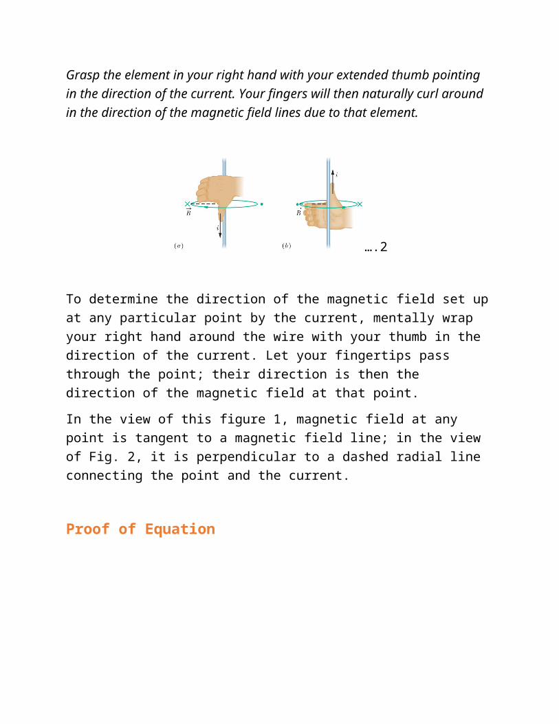
Figure a shows such an arc-shaped wire with central angleφ, radius R, and center C, carrying current i. At C, each current-length element ids of the wire produces a magnetic field of magnitude dB given by Eq. A.

Moreover, as Fig. b shows, no matter where the element is located on the wire, the angle θ between the current-length element vectors and unit vector is 90°; also, r = R. Thus, by substituting R for r and 90° for θ in Eq. A, we obtain

….E

The field at C due to each current-length element in the arc has this magnitude.

Direction of the differential Field

From the previous discussion, we now know that the vector must be perpendicular to a radial line extending through point C from the element, either into the plane or out of it.

To tell which direction is correct, we use the right-hand rule for any of the elements, as shown in Fig. c Grasping the wire with the thumb in the direction of the current and bringing the fingers into the region near C, we see that the differential field vector due to any of the differential elements is out of the plane of the figure, not into it.

To find the total field at C due to all the elements on the arc, we need to add all the differential magnetic field vectors. However, because the vectors are all in the same direction, we do not need to find components. We just sum the magnitudes of field vectors i.e. dB as given by Eq. E. Since we have a vast number of those magnitudes, we sum via integration. We want the result to indicate how the total field depends on the angle of the arc (rather than the arc length).

So, in Eq. E we switch from ds to dϕ by using the identity

ds=R dϕ.

The summation by integration is then given by this equation

Integrating, we find that

B=μ0 iϕ4 πR

Force between Two Parallel Currents

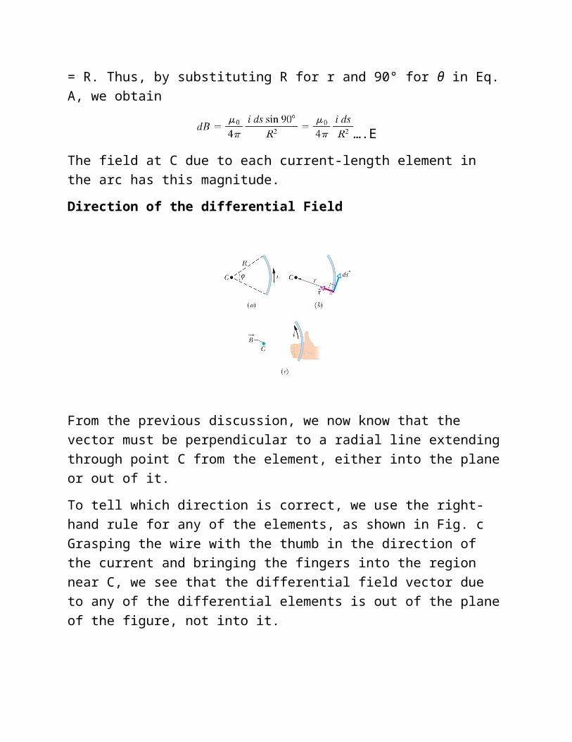
Two long parallel wires carrying currents exert forces on each other. The Figure here shows two such wires, separated by a distance d and carrying currents ia and ib.

Let us analyze the forces on these wires due to each other.

We seek first the force on wire b due to the current in wire a.

That current produces a magnetic field and it is this magnetic field that actually causes the force we seek. To find the force, then, we need the magnitude and direction of the field at the site of wire b. The magnitude of magnetic field at every point of wire b is, then,

The curled–straight right-hand rule tells us that the direction of magnetic field due to wire a at wire b is down. Now that we have the field, we can find the force it produces on wire b. The force on a length L of wire b due to the external magnetic field produced by wire a is

In Fig., vectors L and Ba are perpendicular to each other, so, we can write

The direction of force vector is the direction of the cross product of the length of wire and the magnetic field due to wire a. applying the right-hand rule for cross

products to the length of wire and the magnetic field in, we see that the force is directly toward wire a.

The general procedure for finding the force on a current-carrying wire is this:

To find the force on a current-carrying wire due to a second current-carrying wire, first find the field due to the second wire at the site of the first wire. Then find the force on the first wire due to that field.

We could now use this procedure to compute the force on wire ‘a” due to the current in wire ‘b’. We would find that the force is directly toward wire ‘b’; hence, the two wires with parallel currents attract each other. Similarly, if the two currents were antiparallel, we could show that the two wires repel each other.

So friends here we come to the end of our discussion in this lecture today and therefore we sum

The magnetic field set up by a current-carrying conductor can be found from the Biot – Savart law.

For a long straight wire carrying a current i, the Biot – Savart law gives, for the magnitude of the magnetic field at a perpendicular distance R from the wire.

Parallel wires carrying currents in the same direction attract each other, whereas parallel wires carrying currents in opposite directions repel each other.

So that is it for today. See you in the next lecture where we shall be discussing Ampere’s Law.

Thank you very much.

OBJECTIVE

The objective of this lecture is to make the students of B.Sc. Computers understand the Biot-Savart Law.

Course : Bachelor of Applied Physical Science

IInd Year (Semester IV)

Paper no : 14

Subject : PHPT – 404 Electricity, Magnetism and

Electromagnetic Theory

Topic No. & Title : Topic – 1 Electrostatics

Lecture No : 12

Tittle : Biot - Savart Law

SUMMARY

The magnetic field set up by a current-carrying conductor can be found from the Biot – Savart law.

For a long straight wire carrying a current i, the Biot – Savart law gives, for the magnitude of the magnetic field at a perpendicular distance R from the wire.

Parallel wires carrying currents in the same direction attract each other, whereas parallel wires carrying currents in opposite directions repel each other.

Course : Bachelor of Applied Physical Science

IInd Year (Semester IV)

Paper no : 14

Subject : PHPT – 404 Electricity, Magnetism and

Electromagnetic Theory

Topic No. & Title : Topic – 1 Electrostatics

Lecture No : 12

Tittle : Biot - Savart LawFAQs

Question 1: What is Biot-Savart Law ?

Ans : Biot–Savart law is an equation describing the magnetic field generated by an electric current. It relates the magnetic field to the magnitude, direction, length, and proximity of the electric current. The Biot-Savart Law is much, more accurate than Ampere's Law. The Biot--Savart law can be used in the calculation of magnetic responses even at the atomic or molecular level, e.g. chemical shielding or magnetic susceptibilities, provided that the current density can be obtained from a quantum mechanical calculation or theory.

Question 2: Compare Coulomb’s laws and Biot Savart laws.

Ans : According to coulomb’s law, the magnitude of electric field at any point P depends only on the distance of the charge element from any point P .According to Biot-Savart law, the direction of magnetic field is perpendicular to the current element as well as to the line joining the current element to the point P.

Question 3: What is the general procedure for finding the force on a current-carrying wire ?

Ans : To find the force on a current-carrying wire due to a second current-carrying wire, first find the field due to the second wire at the site of the first wire. Then find the force on the first wire due to that field.

Question 4: What is the right hand rule ?

Ans :The right-hand rule is a common mnemonic for understanding notation conventions for vectors in 3 dimensions. When choosing three vectors that must be at right angles to each other, there are two distinct solutions. This can be seen by holding your hands together, palm up, with the fingers curled. If the curl of your fingers represents a rotation from the first axis to the second, then the third axis can point either along your right thumb or your left thumb.

1. Each of the two long straight parallel wires of negligible cross section placed in vacuum at a distance of 1 meter from each other carries a current of 2 amperes. The force per unit length between the wires is:

1. 1 x 10–7 Newton

2. 2 x 10–7 Newton

3. 4 x 10–7 Newton

4. 8 x 10–7 Newton

2. An electron enters a region of uniform magnetic field with a certain velocity in the direction of the filed. It will move:

1. Along the direction of the filed with unchanged velocity

2. Along the direction on filed with decreasing velocity

3. Along the direction of filed with increasing velocity

4. In a circle with constant speed

3. The tangent galvanometer is called so because:

1. It was invented by Tangent

2. It remain tangential to earth’s surface

3. It produced a magnetic field tangential to the graduated circle

4. It works on the principle of tangent law

4. The magnetic intensity at the center of a circular coil (radius) carrying a current of 1 ampere is proportional to 

1. r

2. r−1

3. r−2

4. r+2

Course : Bachelor of Applied Physical Science

IInd Year (Semester IV)

Paper no : 14

Subject : PHPT – 404 Electricity, Magnetism and

Electromagnetic Theory

Topic No. & Title : Topic – 1 Electrostatics

Lecture No : 12

Tittle : Biot - Savart Law

Glossary

Electric field lines are drawn to represent the electric field;

Density of the lines represents the magnitude of the electric field

Ferromagnetic means having magnetic properties like those of iron

Electric field is a three-dimensional region of electrostatic influence surrounding a charged object

Magnetic field is the three-dimensional region of magnetic influence surrounding a magnet, in which other magnets are affected by magnetic forces

Assignment

Sketch the field lines around the cross-section of two parallel wires when the current in each wire flows

a) In the same direction.

b) In opposite directions.

Course : Bachelor of Applied Physical Science

IInd Year (Semester IV)

Paper no : 14

Subject : PHPT – 404 Electricity, Magnetism and

Electromagnetic Theory

Topic No. & Title : Topic – 1 Electrostatics

Lecture No : 12

Tittle : Biot - Savart Law

References1. Fundamentals of electricity and magnetism By Arthur F. Kip (McGraw-Hill, 1968)

2. Electricity and magnetism by J.H.Fewkes & John Yarwood. Vol. I (Oxford Univ. Press, 1991).

3. Introduction to Electrodynamics, 3rd edition, by David J. Griffiths, (Benjamin Cummings,1998).

4. Electricity and magnetism By Edward M. Purcell (McGraw-Hill Education, 1986)

5. Electricity and magnetism. By D C Tayal (Himalaya Publishing House,1988)

6. Electromagnetics by Joseph A.Edminister 2nd ed.(New Delhi: Tata Mc

Graw Hill, 2006).

Links

http://phun.physics.virginia.edu/topics/electrostatics.html

http://www.sciencedirect.com/science/journal/

http://web.mit.edu/8.02t/www/802TEAL3D/visualizations/electrostatics/