”Babes-Bolyai” University of Cluj-Napoca

Faculty of Mathematics and Computer Science

Summary of the PhD thesis

The Abstract Gronwall Lemma and Applications

by

Cecilia-Florina Craciun

PhD supervisor

Prof. Dr. Ioan A. Rus

2010

Contents

1 Introduction 6

2 Preliminaries 9

2.1 L-spaces . . . . . . . . . . . . . . . . . . . . . . . . . . . . . . . . . . . . . 9

2.2 Metric Fixed Point Theorems . . . . . . . . . . . . . . . . . . . . . . . . . 9

2.3 Picard and Weakly Picard Operators . . . . . . . . . . . . . . . . . . . . . 9

2.4 Abstract Gronwall Lemmas . . . . . . . . . . . . . . . . . . . . . . . . . . 9

2.5 Abstract Comparison Lemmas . . . . . . . . . . . . . . . . . . . . . . . . 10

2.6 Integral Equations and Inequalities in Banach Spaces . . . . . . . . . . . . 10

3 Consequences of the Abstract Gronwall Lemma 11

3.1 Volterra Integral Inequalities . . . . . . . . . . . . . . . . . . . . . . . . . . 11

3.1.1 The Space C([α, β] ,B) . . . . . . . . . . . . . . . . . . . . . . . . . 12

3.1.2 The Space C([α, β] ,R) . . . . . . . . . . . . . . . . . . . . . . . . . 13

3.1.3 The Space C ([α, β] ,Rp) . . . . . . . . . . . . . . . . . . . . . . . . 14

3.1.4 The Spaces C([α, β], l2(R)) and C([α, β], s(R)) . . . . . . . . . . . . 14

3.2 Fredholm Integral Inequalities . . . . . . . . . . . . . . . . . . . . . . . . . 16

3.2.1 The Space C([α, β] ,B) . . . . . . . . . . . . . . . . . . . . . . . . . 17

3.2.2 The Space C([α, β] ,R) . . . . . . . . . . . . . . . . . . . . . . . . . 18

3.2.3 The Space C([α, β] ,Rp) . . . . . . . . . . . . . . . . . . . . . . . . 18

3.2.4 The Spaces C([α, β], l2(R)) and C([α, β], s(R)) . . . . . . . . . . . . 18

3.3 Integral Inequalities with Modified Argument . . . . . . . . . . . . . . . . 20

2

3.4 Multi-dimensional Integral Inequalities . . . . . . . . . . . . . . . . . . . . 20

3.5 Volterra-Fredholm Integral Inequalities . . . . . . . . . . . . . . . . . . . . 21

4 Applications to Optimality Results 27

4.1 Optimality Results in Explicit Form . . . . . . . . . . . . . . . . . . . . . . 27

4.2 Optimality Results in Generic Form . . . . . . . . . . . . . . . . . . . . . . 31

5 Applications to the Study of Solutions and to Stability 34

5.1 Applications to the Study of Solutions to Various Inequalities . . . . . . . 34

5.1.1 Second-order Hyperbolic Inequalities . . . . . . . . . . . . . . . . . 35

5.1.2 Third-order Hyperbolic Inequalities . . . . . . . . . . . . . . . . . . 35

5.1.3 Pseudoparabolic Inequalities . . . . . . . . . . . . . . . . . . . . . . 36

5.2 Applications to Ulam Stabilities of Hyperbolic Equations . . . . . . . . . . 38

Bibliography 42

3

Abstract

In this thesis we derive optimal bounds (explicitly or in a generic form) for

the solutions to integral or differential inequalities. We re-write the equations and

inequalities in terms of integral operators. Applying the Abstract Gronwall Lemma

to these operators gives the optimal bounds. We also present some applications

of the Abstract Gronwall Lemma to pseudoparabolic and second and third-order

hyperbolic inequalities, as well as to the study of Ulam stabilities for the second-

order differential equations of hyperbolic type.

Keywords

Fixed Point Theory, Picard Operators, Abstract Gronwall Lemma, Comparison

Lemma, Integral Equations, Integral Inequalities, Volterra Integral Inequalities,

Fredholm Integral Inequalities, Triangular Operators, Hyperbolic Inequalities, Pseu-

doparabolic Inequalities, Ulam Stabilities.

4

Acknowledgements

First of all, I am deeply thankful to my PhD supervisor, Prof. Dr. Ioan A. Rus, who

has always been helpful and has offered invaluable suggestions, support and guidance. His

confidence has inspired me when I doubted myself, and he has constantly encouraged me

throughout this work.

I am also very grateful to Prof. Dr. N. Lungu and Dr. M.A. Serban for their collab-

oration in our joint articles, and the advice they have given. Their support is greatly

appreciated.

My thanks also go to all the members of the Applied Mathematics Department of

Babes-Bolyai University for all their kind assistance with this work.

I also want to thank the librarians for providing me with books and articles.

Last, but not least, I wish to express my loving thanks to my family and friends. Their

love, encouragement and understanding have helped me immeasurably.

5

Chapter 1

Introduction

Integral equations are an important part of Pure and Applied Mathematics, with appli-

cations in differential equations, mechanical vibrations, engineering, physics, numerical

computations and others (see, for instance, [66] and [99]). The beginning of the theory of

Integral Equations can be attributed to N. H. Abel who formulated an integral equation

in 1812 when studying a problem in Mechanics. Since then many other great mathemati-

cians including T. Lalescu (who wrote the first dissertation on Integral Equations in the

world in 1911, see [42]), J. Liouville, J. Hadamard, V. Volterra, I. Fredholm, E. Gour-

sat, D. Hilbert, E Picard, H. Poincare have contributed to the development of Integral

Equations.

Gronwall-type lemmas play an important role in the area of Integral (and Differential)

Equations, as technical tools used to prove existence and uniqueness of a solution and to

obtain various estimates for the solutions. They can be viewed as a type of result which

gives a priori bounds for the function which satisfies an integral or differential inequality.

In this thesis we use Gronwall-type lemmas to obtain bounds of the functions that

satisfy a certain differential or integral inequality, and express these bounds as fixed

points of the corresponding integral operators.

In a recent paper [86], I.A. Rus has formulated ten problems of interest in the theory

of Gronwall lemmas. One of them concerns finding examples of Gronwall-type lemmas in

which the upper bounds are fixed points of the corresponding operator A (Problem 5).

6

Another problem is identifying which of these Gronwall-type lemmas can be obtained as

consequences of the Abstract Gronwall Lemma (Problem 6). Abstract Gronwall Lemma

gives the lowest majorant among all possible upper bounds (see [84]). There is no general

methodology to answer these questions, so they have to be obtained on case-by-case basis.

Over the years many mathematicians have obtained such examples (see, for instance, [8],

[22], [25], [55], [57], [83], [84], [86]), and this work presents more such results.

The second chapter is dedicated to notations, definitions, lemmas and theorems, which

will be used in the subsequent chapters.

In the third chapter we study some consequences of the Abstract Gronwall Lemma in

the cases of Volterra and Fredholm integral inequalities in Banach and non-Banach spaces.

In general, it is difficult to find the exact solutions to the integral equations or bounds

for the functions which satisfy integral inequalities; therefore we need to apply results

from fixed point theory and the Picard operators technique to prove existence of solutions

and to find some bounds for these solutions. We also present some particular examples

of integral inequalities in the Banach spaces C([α, β],R) and C([α, β],Rp), and study the

case of infinite systems of integral equations in the space C([α, β], s(R)) and the Banach

space C([α, β], l2(R)), respectively. The results of this chapter have been published in [22]

and [25].

In the fourth chapter we investigate some integral inequalities studied in [8], [41],

[45], [57], for which the authors obtained bounds for the solutions using various methods.

Applying the Abstract Gronwall Lemma we are able to show that their bounds are optimal

or, when that is not the case, we obtain ourselves the optimal bounds. Furthermore, we

prove that our bounds are lowest ones among all possible upper bounds, hence they are

optimal. Some optimal bounds are expressed explicitly and others just in a generic form.

The results of this chapter have been published in [21], [22] and [25].

In the last chapter we apply the Abstract Gronwall Lemma to second and third-order

hyperbolic inequalities and pseudoparabolic inequalities. Adding boundary conditions to

hyperbolic and pseudoparabolic equations results in Darboux problems. We use the Pi-

card operators technique to prove the existence and the uniqueness of the solution to

7

these Darboux problems, and we apply the Abstract Gronwall Lemma to functions that

satisfy the corresponding inequalities. We also use the Riemann function to represent the

solutions to these Darboux problems in the case of specific pseudoparabolic inequalities.

We conclude this chapter with a study of the Ulam stabilities for the second-order differ-

ential equations of hyperbolic type. The articles [23] and [24] contain the main results of

this last chapter.

8

Chapter 2

Preliminaries

The aim of this chapter is to present some notions and results which are necessary in the

derivation of the original results of this thesis. These results can be found in the following

references: [20], [31], [55], [56], [66], [76], [79], [81], [83], [86], [91], [92], [99].

The metric fixed point theorems guarantee the existence and uniqueness of fixed points

of certain well defined operators in metric spaces, and usually provide a constructive

method to find those fixed points. The results presented in this section can be found in:

[12], [26], [37], [39], [74], [78], [81], [82], [84], [85], [91] and others.

We consider the Chebyshev and Bielecki norms, which are metrically equivalent:

‖x‖C : = maxt∈[α,β]

|x(t)| , (2.0.1)

‖x‖τ : = maxt∈[α,β]

(|x(t)| exp(−τ(t− α))), τ ∈ R∗+ (2.0.2)

With respect to these norms C ([α, β] ,B) is a Banach space.

The standard tool for proving the existence and uniqueness, data dependance and

comparison results for the solution to integral equations is the Picard operators technique.

Following [83] we present the basic notions and results from the Picard and Weakly

Picard Operators theory (see also [22], [23], [25], [33], [64], [78], [81], [82], [84], [91]).

Gronwall lemmas are the subject of this thesis, and we use them to bound a function

that satisfies a certain differential or integral inequality by the solution of the correspond-

ing differential or integral equation. The following abstract lemmas are the main tools for

9

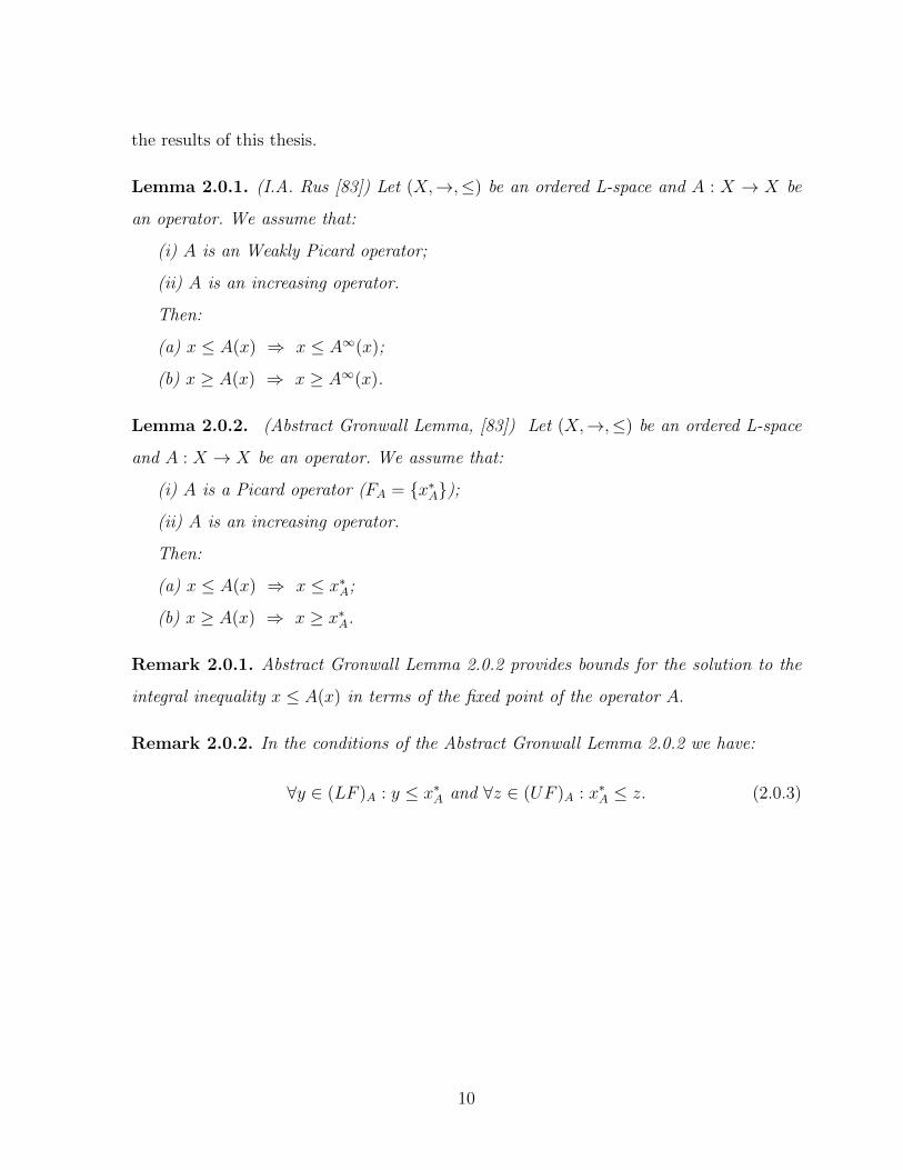
the results of this thesis.

Lemma 2.0.1. (I.A. Rus [83]) Let (X,→,≤) be an ordered L-space and A : X → X be

an operator. We assume that:

(i) A is an Weakly Picard operator;

(ii) A is an increasing operator.

Then:

(a) x ≤ A(x) ⇒ x ≤ A∞(x);

(b) x ≥ A(x) ⇒ x ≥ A∞(x).

Lemma 2.0.2. (Abstract Gronwall Lemma, [83]) Let (X,→,≤) be an ordered L-space

and A : X → X be an operator. We assume that:

(i) A is a Picard operator (FA = {x∗A});

(ii) A is an increasing operator.

Then:

(a) x ≤ A(x) ⇒ x ≤ x∗A;

(b) x ≥ A(x) ⇒ x ≥ x∗A.

Remark 2.0.1. Abstract Gronwall Lemma 2.0.2 provides bounds for the solution to the

integral inequality x ≤ A(x) in terms of the fixed point of the operator A.

Remark 2.0.2. In the conditions of the Abstract Gronwall Lemma 2.0.2 we have:

∀y ∈ (LF )A : y ≤ x∗A and ∀z ∈ (UF )A : x∗A ≤ z. (2.0.3)

10

Chapter 3

Consequences of the Abstract

Gronwall Lemma

The Picard operators and Gronwall type lemmas play a significant role in the qualitative

theory of integral equations. In this chapter we study some consequences of Abstract

Gronwall Lemma 2.0.2 in the cases of Volterra and Fredholm integral inequalities in

Banach spaces. In general it is difficult to find the exact solutions of the integral equations

and inequalities. The fixed point theory and the Picard operators technique allow us to

prove the existence and, furthermore, to find some bounds of these solutions. We also

present some particular examples of integral inequalities in C([α, β], s(R)) and in the

Banach spaces C([α, β],R), C([α, β],Rp) and C([α, β], l2(R)) respectively.

The original results of this chapter have been published in [22] and [25].

3.1 Volterra Integral Inequalities

Volterra integral equations and inequalities have been studied for many years in Applied

Mathematics using both, the classical and the fixed-point technique methods.

In this section we present a general result for Volterra operators in Banach spaces,

and then particular results for the cases of Banach spaces C([α, β],R), C([α, β],Rp) and

11

C([α, β], l2(R)), and also for triangular operators in the non-Banach space C([α, β], s(R)).

In some cases, the fixed points of the corresponding operators can be determined.

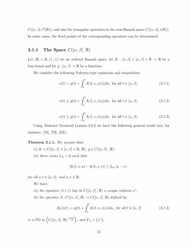
3.1.1 The Space C([α, β] ,B)

Let (B,+,R, |·| ,≤) be an ordered Banach space, let K : [α, β] × [α, β] × B → B be a

functional and let g : [α, β]→ B be a function.

We consider the following Volterra-type equations and inequalities:

x(t) = g(t) +

∫ t

α

K(t, s, x(s))ds, for all t ∈ [α, β] , (3.1.1)

x(t) ≤ g(t) +

∫ t

α

K(t, s, x(s))ds, for all t ∈ [α, β] , (3.1.2)

x(t) ≥ g(t) +

∫ t

α

K(t, s, x(s))ds, for all t ∈ [α, β] . (3.1.3)

Using Abstract Gronwall Lemma 2.0.2 we have the following general result (see, for

instance, [78], [79], [83]):

Theorem 3.1.1. We assume that:

(i) K ∈ C([α, β]× [α, β]× B, B), g ∈ C([α, β] , B);

(ii) there exists LK > 0 such that:

|K(t, s, u)−K(t, s, v)| ≤ LK |u− v| ,

for all s, t ∈ [α, β], and u, v ∈ B;

We have:

(a) the equation (3.1.1) has in C([α, β] , B) a unique solution x∗;

(b) the operator A : C([α, β] ,B)→ C([α, β] ,B) defined by:

A(x)(t) := g(t) +

∫ t

α

K(t, s, x(s))ds, for all t ∈ [α, β] (3.1.4)

is a PO in(C([α, β] ,B),

unif→), and FA = {x∗}.

12

If in addition we have the hypothesis:

(iii) K(t, s, ·) : B→ B is increasing, for all t, s ∈ [α, β],

then:

(c) if x ∈ C([α, β] , B) satisfies the inequality (3.1.2), then x(t) ≤ x∗(t), for all t ∈

[α, β];

(d) if x ∈ C([α, β] , B) satisfies the inequality (3.1.3), then x(t) ≥ x∗(t), for all t ∈

[α, β].

Remark 3.1.1. The above theorem is well known, but it is very useful for understanding

our results.

3.1.2 The Space C([α, β] ,R)

In this subsection we start by considering the particular case of Theorem 3.1.1 when

B := R. Then we apply this theorem to the case when the functional K is linear, i.e.

K(t, s, u) = k(t, s)u, for all t, s ∈ [α, β], and u ∈ R. In this case the solution x∗ is given

in terms of the resolvent kernel.

In general it is difficult to work out an explicit expression of the resolvent kernel. For

some particular cases, the integral equations can be solved and explicit forms of the kernel

can be obtained. Such examples are represented, for instance, by Gronwall’s Lemma and

Filatov’s Theorem (see [8], [22], [51] and others)

As in the linear case of the functional K, in the nonlinear one it is difficult to solve the

corresponding integral equations in order to find bounds of the solutions. There are some

specific Gronwall lemmas in which the fixed point of the corresponding operator can be

determined. In what follows we present an example of such lemma.

Theorem 3.1.2. (Bihari-type inequality)([22], see also [56], [96]) We assume that:

(i) c ∈ R, p ∈ C([α, β],R+)

(ii) V is a continuous, positive, increasing, and Lipschitz function.

We have :

13

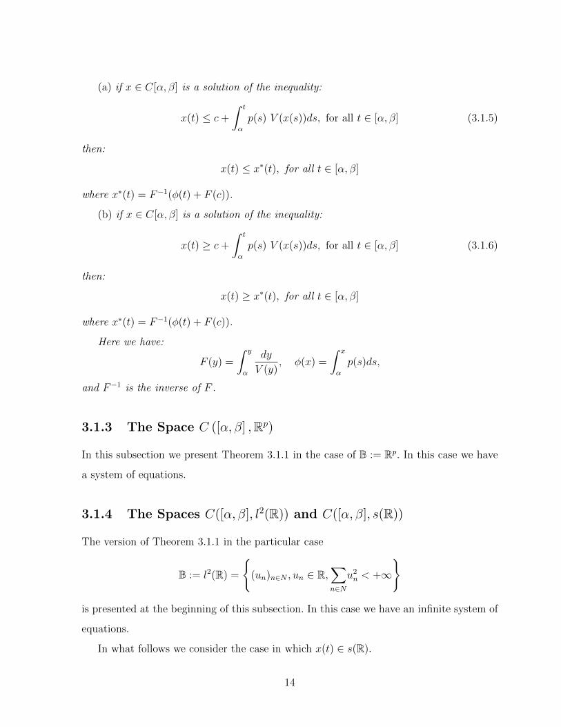
(a) if x ∈ C[α, β] is a solution of the inequality:

x(t) ≤ c+

∫ t

α

p(s) V (x(s))ds, for all t ∈ [α, β] (3.1.5)

then:

x(t) ≤ x∗(t), for all t ∈ [α, β]

where x∗(t) = F−1(φ(t) + F (c)).

(b) if x ∈ C[α, β] is a solution of the inequality:

x(t) ≥ c+

∫ t

α

p(s) V (x(s))ds, for all t ∈ [α, β] (3.1.6)

then:

x(t) ≥ x∗(t), for all t ∈ [α, β]

where x∗(t) = F−1(φ(t) + F (c)).

Here we have:

F (y) =

∫ y

α

dy

V (y), φ(x) =

∫ x

α

p(s)ds,

and F−1 is the inverse of F .

3.1.3 The Space C ([α, β] ,Rp)

In this subsection we present Theorem 3.1.1 in the case of B := Rp. In this case we have

a system of equations.

3.1.4 The Spaces C([α, β], l2(R)) and C([α, β], s(R))

The version of Theorem 3.1.1 in the particular case

B := l2(R) =

{(un)n∈N , un ∈ R,

∑n∈N

u2n < +∞

}

is presented at the beginning of this subsection. In this case we have an infinite system of

equations.

In what follows we consider the case in which x(t) ∈ s(R).

14

We obtain an infinite system of integral equations:

x0(t) = g0(t) +∫ tαK0(t, s, x0(s))ds

x1(t) = g1(t) +∫ tαK1(t, s, x0(s), x1(s))ds

......................................................

xp(t) = gp(t) +∫ tαKp(t, s, x0(s), x1(s), ..., xp(s))ds

......................................................,

(3.1.7)

for all t ∈ [α, β] , where Kn : [α, β]× [α, β]× Rn+1 → R,∀n ∈ N and g : [α, β]→ s(R).

We consider Xn := C[α, β], n ∈ N and the operators

An :n∏i=0

Xi → Xn, defined by:

A0(x0)(t) := g0(t) +∫ tαK0(t, s, x0(s))ds,

An(x0, x1, ..., xn)(t) := gn(t) +∫ tαKn(t, s, x0(s), x1(s), ..., xn(s))ds.

(3.1.8)

We denote by X :=∏i∈N

Xi and

A : X → X, A = (A0, A1, ..., Ap, ...), (3.1.9)

where A0, ..., Ap, ... are given by (3.1.8).

The existence and the uniqueness of the solution to the infinite system (3.1.7) have

been obtained by I. A. Rus and M. A. Serban in [93]. We add the monotony condition

for the functionals Kn, n ∈ N, and applying the Abstract Gronwall Lemma 2.0.2 gives us

the following theorem:

Theorem 3.1.3. We assume that:

(i) gn ∈ C[α, β], Kn ∈ C([α, β]× [α, β]× Rn+1), n ∈ N;

(ii) there exists LK0 > 0 such that:

|K0(t, s, ξ1)−K0(t, s, ξ2)| ≤ LK0 |ξ1 − ξ2| , (3.1.10)

for all t, s ∈ [α, β], ξ1, ξ2 ∈ R;

15

(iii) there exists LKn > 0 such that:

|Kn(t, s, u0, u1, ..., un−1, ξ1)−Kn(t, s, u0, u1, ..., un−1, ξ2)| ≤ LKn |ξ1 − ξ2| , (3.1.11)

for all t, s ∈ [α, β], u0, u1, ..., un−1, ξ1, ξ2 ∈ R, p ∈ N∗.

Then:

(a) the infinite system (3.1.7) has a unique solution x∗ ∈ C([α, β] , s(R));

(b) the corresponding operator A defined by (3.1.9) is a PO in (C([α, β] , s(R)),t→).

If in addition we have the hypothesis:

(iv) Kn(t, s, ·, ..., ·) : Rn+1 → R is increasing for all t, s ∈ [α, β] and ∀n ∈ N,

then:

(c) if x ∈ C([α, β] , s(R)) satisfies the corresponding inequality (3.1.2), then x(t) ≤

x∗(t), for all t ∈ [α, β];

(d) if x ∈ C([α, β] , s(R)) satisfies the corresponding inequality (3.1.3), then x(t) ≥

x∗(t), for all t ∈ [α, β].

3.2 Fredholm Integral Inequalities

Along with Volterra integral equations and inequalities, the integral inequalities of Fred-

holm type play an essential role in the nonlinear analysis. The Fredholm equations and

inequalities have been studied by many mathematicians over the years. Some monographs

on Fredholm equations have been written by D. Bainov and P. Simeonov (see [8]), C. Cor-

duneanu (see [20]), D.S. Mitrinovic, J.E. Pecaric, A.M. Fink (see [51]). See also: Sz. Andras

([1], [2]), F. Calio, E. Marcchetti and V. Muresan ([14]), C. Craciun and N. Lungu ([22]),

V. Muresan ([52]), B.G. Pachpatte ([56], [55]), I.A. Rus ([76], [78], [81], [84], [86],[85],

[83]), N. Taghizadeh and V. Khanbabai ([98]).

In this section we present a Gronwall-type lemma for Fredholm operators in Ba-

nach spaces, and then particular results for the cases of Banach spaces C([α, β],R),

C([α, β],Rp) and C([α, β], l2(R)), and also for triangular operators in the non-Banach

space C([α, β], s(R)).

16

3.2.1 The Space C([α, β] ,B)

Let (B,+,R, |·| ,≤) be an ordered Banach space, let H : [α, β] × [α, β] × B → B be a

functional, and let g : [α, β]→ B be a function.

We consider the following Fredholm-type equation and inequalities:

x(t) = g(t) +

∫ β

α

H(t, s, x(s))ds, for all t ∈ [α, β] , (3.2.1)

x(t) ≤ g(t) +

∫ β

α

H(t, s, x(s))ds, for all t ∈ [α, β] , (3.2.2)

x(t) ≥ g(t) +

∫ β

α

H(t, s, x(s))ds, for all t ∈ [α, β] . (3.2.3)

Theorem 3.2.1. We assume that:

(i) H ∈ C([α, β]× [α, β]× B, B), g ∈ C([α, β] , B);

(ii) there exists LH > 0 such that:

|H(t, s, u)−H(t, s, v)| ≤ LH |u− v| ,

for all s, t ∈ [α, β], and u, v ∈ B;

(iii) LH(β − α) < 1;

We have:

(a) the equation (3.2.1) has in C([α, β] , B) a unique solution x∗;

(b) the operator B : C([α, β] ,B)→ C([α, β] ,B), defined by:

B(x)(t) := g(t) +

∫ β

α

H(t, s, x(s))ds, for all t ∈ [α, β] (3.2.4)

is a PO in(C([α, β] ,B),

unif→), and FB = {x∗}.

If in addition we have the hypothesis:

(iv) H(t, s, ·) : B→ B is increasing for all t, s ∈ [α, β],

then:

(c) if x ∈ C([α, β] , B) satisfies the inequality (3.2.2), then:

x(t) ≤ x∗(t), for all t ∈ [α, β] ; (3.2.5)

(d) if x ∈ C([a, b] , B) satisfies the inequality (3.2.3), then:

x(t) ≥ x∗(t), for all t ∈ [α, β] . (3.2.6)

17

3.2.2 The Space C([α, β] ,R)

We start this case by considering the linear form of the functional H, i.e. H(t, s, u) :=

h(t, s)u, case for which we present a Gronwall-type result.

Remark 3.2.1. If the integral equation has a degenerate kernel, i.e. h(t, s) =

p∑i=1

ai(t)

bi(s), where a and b are continuous functions on [α, β], then the solution to the integral

equation is, in fact, the solution of an algebraic system, which can be found explicitly.

3.2.3 The Space C([α, β] ,Rp)

If B := Rp the equation (3.2.1) is, in fact, a system of equations. A Gronwall-type result

for this system is presented in this subsection.

3.2.4 The Spaces C([α, β], l2(R)) and C([α, β], s(R))

The first part of this subsection consists of a Gronwall-type result for Fredholm equation

and inequalities in the particular case of C([α, β], l2(R)).

The case of C([α, β], s(R)) follows. Here we have the following infinite system of inte-

gral equations:

x0(t) = g0(t) +∫ βαH0(t, s, x0(s))ds

x1(t) = g1(t) +∫ βαH1(t, s, x0(s), x1(s))ds

...................................................... for all t ∈ [α, β]

xp(t) = gp(t) +∫ βαHp(t, s, x0(s), x1(s), ..., xp(s))ds

......................................................,

(3.2.7)

where Hn : [α, β]× [α, β]× Rn+1 → R, ∀n ∈ N and g : [α, β]→ s(R).

For any n ∈ N we consider Xn := C[α, β] and the operators

Bn :n∏i=0

Xi → Xn, defined by:

18

B0(x0)(t) := g0(t) +∫ βαH0(t, s, x0(s))ds,

Bn(x0, x1, ..., xn)(t) := gn(t) +∫ βαHn(t, s, x0(s), x1(s), ..., xn(s))ds.

(3.2.8)

We denote by X :=∏i∈N

Xi and

B : X → X, B = (B0, B1, ..., Bp, ...), (3.2.9)

where B0, ..., Bp, ... are given by (3.2.8).

From Theorem 3.2.1 we obtain theoretical bounds for functions which satisfy the

corresponding inequalities (3.2.2) and (3.2.3) in the case of triangular operators. These

functions are dominated by the fixed point of the corresponding operator.

Theorem 3.2.2. We assume that:

(i) gn ∈ C[α, β], Hn ∈ C([α, β]× [α, β]× Rn+1), ∀n ∈ N;

(ii) there exists LH0 > 0 such that:

|H0(t, s, ξ1)−H0(t, s, ξ2)| ≤ LH0 |ξ1 − ξ2| , (3.2.10)

for all t, s ∈ [α, β], ξ1, ξ2 ∈ R;

(iii) LH0(β − α) < 1;

(iv) there exists LHn > 0 such that:

|Hn(t, s, u0, u1, ..., un−1, ξ1)−Hn(t, s, u0, u1, ..., un−1, ξ2)| ≤ LHn |ξ1 − ξ2| , (3.2.11)

for all t, s ∈ [α, β], u0, u1, ..., un−1, ξ1, ξ2 ∈ R, n ∈ N∗;

(v) LHn(β − α) < 1, ∀n ∈ N∗;

We have:

(a) the infinite system (3.2.7) has a unique solution x∗ ∈ C([α, β] , s(R));

(b) the corresponding operator B defined by (3.2.9) is a PO in (C([α, β] , s(R)),t→)

and FB = {x∗}.

If in addition we have the hypothesis:

(vi) Hn(t, s, ·, ..., ·) : Rn+1 → R is increasing for all t, s ∈ [α, β] and ∀n ∈ N,

19

then:

(c) if x ∈ C([α, β] , s(R)) satisfies the corresponding inequality (3.1.2), then x(t) ≤

x∗(t), for all t ∈ [α, β];

(d) if x ∈ C([α, β] , s(R)) satisfies the corresponding inequality (3.1.3), then x(t) ≥

x∗(t), for all t ∈ [α, β].

3.3 Integral Inequalities with Modified Argument

Integral inequalities with modified argument are used to describe many phenomena in

science, economics, population dynamics, physics, medicine etc. They have been studied

by many researchers: D. Bainov and P. Simeonov [8], T.A. Burton [13], M. Dobritoiu [27],

[28], M. Dobritoiu, I.A. Rus and M.A. Serban [29], D. Guo, V. Lakshmikantham and X.

Liu [33], N. Lungu [46], D.S. Mitrinovic, J.E. Pecaric and A.M. Fink [51], V. Muresan

[53], B.G. Pachpatte [56], R. Precup and E. Kirr [71], and others.

In this section are presented Gronwall-type results, in both cases, Volterra and

Fredholm-type equations and inequalities.

3.4 Multi-dimensional Integral Inequalities

Similar results to those presented in sections 3.1 and 3.2 can be obtained in the case of

multi-dimensional integral inequalities (see, for instance, [8], [9], [56]). These inequalities

can be used in the study of various problems in the theory of certain partial differen-

tial, integral and integro-differential equations, especially in the study of the qualitative

behaviour of the solutions.

20

3.5 Volterra-Fredholm Integral Inequalities

In this section we consider the following mixed type Volterra-Fredholm nonlinear integral

equation and inequalities:

x (t) = F

(t, x(t),

∫ t1

α1

. . .

∫ tm

αm

K(t, s, x(s))ds,

∫ β1

α1

. . .

∫ βm

αm

H(t, s, x(s))ds

), (3.5.1)

x (t) ≤ F

(t, x(t),

∫ t1

α1

. . .

∫ tm

αm

K(t, s, x(s))ds,

∫ β1

α1

. . .

∫ βm

αm

H(t, s, x(s))ds

), (3.5.2)

x (t) ≥ F

(t, x(t),

∫ t1

α1

. . .

∫ tm

αm

K(t, s, x(s))ds,

∫ β1

α1

. . .

∫ βm

αm

H(t, s, x(s))ds

), (3.5.3)

where [α1; β1]×. . .×[αm; βm] is an interval in Rm, K,H : [α1; β1]×. . .×[αm; βm]×[α1; β1]×

. . .× [αm; βm]×R→ R are continuous functions and F : [α1; β1]× . . .× [αm; βm]×R3→ R

is a functional. The mixed type Volterra-Fredholm integral equations have been studied

by many authors (see [2], [55], [63], [94], [95] and others).

We prove the existence and uniqueness for the solution of integral equation (3.5.1)

by standard techniques as in [2], [14], [22], [47], our integral equation (3.5.1) being more

general than integral equations considered in above mentioned papers. We also establish a

Gronwall-type lemma for these inequalities. The results of this section have been published

in [25].

Theorem 3.5.1. ([25]) We assume that:

(i) K, H ∈ C([α1, β1]× · · · × [αm, βm]× [α1, β1]× · · · × [αm, βm]× R);

(ii) F ∈ C([α1, β1]× · · · × [αm, βm]× R3);

(iii) there exist a, b, c nonnegative constants such that:

|F (t, u1, v1, w1)− F (t, u2, v2, w2)| ≤ a|u1 − u2|+ b|v1 − v2|+ c|w1 − w2|,

for all t ∈ [α1, β1]× · · · × [αm, βm], u1, u2, v1, v2, w1, w2 ∈ R;

21

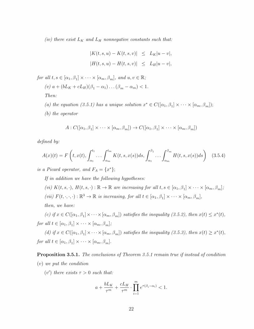
(iv) there exist LK and LH nonnegative constants such that:

|K(t, s, u)−K(t, s, v)| ≤ LK |u− v|,

|H(t, s, u)−H(t, s, v)| ≤ LH |u− v|,

for all t, s ∈ [α1, β1]× · · · × [αm, βm], and u, v ∈ R;

(v) a+ (bLK + cLH)(β1 − α1) . . . (βm − αm) < 1.

Then:

(a) the equation (3.5.1) has a unique solution x∗ ∈ C([α1, β1]× · · · × [αm, βm]);

(b) the operator

A : C([α1, β1]× · · · × [αm, βm])→ C([α1, β1]× · · · × [αm, βm])

defined by:

A(x)(t) = F

(t, x(t),

∫ t1

α1

. . .

∫ tm

αm

K(t, s, x(s))ds,

∫ β1

α1

. . .

∫ βm

αm

H(t, s, x(s))ds

)(3.5.4)

is a Picard operator, and FA = {x∗};

If in addition we have the following hypotheses:

(vi) K(t, s, ·), H(t, s, ·) : R→ R are increasing for all t, s ∈ [α1, β1]× · · · × [αm, βm];

(vii) F (t, ·, ·, ·) : R3 → R is increasing, for all t ∈ [α1, β1]× · · · × [αm, βm],

then, we have:

(c) if x ∈ C([α1, β1]×· · ·× [αm, βm]) satisfies the inequality (3.5.2), then x(t) ≤ x∗(t),

for all t ∈ [α1, β1]× · · · × [αm, βm];

(d) if x ∈ C([α1, β1]×· · ·× [αm, βm]) satisfies the inequality (3.5.3), then x(t) ≥ x∗(t),

for all t ∈ [α1, β1]× · · · × [αm, βm].

Proposition 3.5.1. The conclusions of Theorem 3.5.1 remain true if instead of condition

(v) we put the condition

(v′) there exists τ > 0 such that:

a+bLKτm

+cLHτm·m∏i=1

eτ(βi−αi) < 1.

22

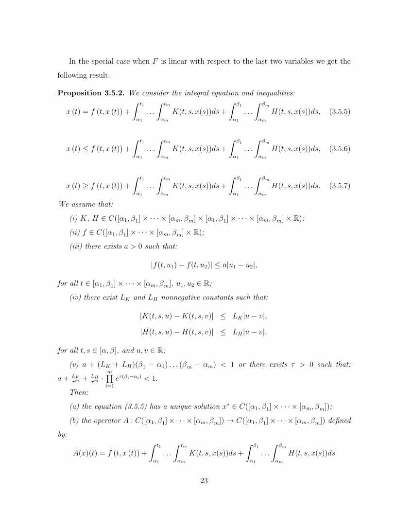
In the special case when F is linear with respect to the last two variables we get the

following result.

Proposition 3.5.2. We consider the integral equation and inequalities:

x (t) = f (t, x (t)) +

∫ t1

α1

. . .

∫ tm

αm

K(t, s, x(s))ds+

∫ β1

α1

. . .

∫ βm

αm

H(t, s, x(s))ds, (3.5.5)

x (t) ≤ f (t, x (t)) +

∫ t1

α1

. . .

∫ tm

αm

K(t, s, x(s))ds+

∫ β1

α1

. . .

∫ βm

αm

H(t, s, x(s))ds, (3.5.6)

x (t) ≥ f (t, x (t)) +

∫ t1

α1

. . .

∫ tm

αm

K(t, s, x(s))ds+

∫ β1

α1

. . .

∫ βm

αm

H(t, s, x(s))ds. (3.5.7)

We assume that:

(i) K, H ∈ C([α1, β1]× · · · × [αm, βm]× [α1, β1]× · · · × [αm, βm]× R);

(ii) f ∈ C([α1, β1]× · · · × [αm, βm]× R);

(iii) there exists a > 0 such that:

|f(t, u1)− f(t, u2)| ≤ a|u1 − u2|,

for all t ∈ [α1, β1]× · · · × [αm, βm], u1, u2 ∈ R;

(iv) there exist LK and LH nonnegative constants such that:

|K(t, s, u)−K(t, s, v)| ≤ LK |u− v|,

|H(t, s, u)−H(t, s, v)| ≤ LH |u− v|,

for all t, s ∈ [α, β], and u, v ∈ R;

(v) a + (LK + LH)(β1 − α1) . . . (βm − αm) < 1 or there exists τ > 0 such that:

a+ LKτm

+ LHτm·m∏i=1

eτ(βi−αi) < 1.

Then:

(a) the equation (3.5.5) has a unique solution x∗ ∈ C([α1, β1]× · · · × [αm, βm]);

(b) the operator A : C([α1, β1]× · · · × [αm, βm])→ C([α1, β1]× · · · × [αm, βm]) defined

by:

A(x)(t) = f (t, x (t)) +

∫ t1

α1

. . .

∫ tm

αm

K(t, s, x(s))ds+

∫ β1

α1

. . .

∫ βm

αm

H(t, s, x(s))ds

23

is a PO, and FA = {x∗}.

If in addition we have the following hypotheses:

(vi) f(t, ·) : R→ R is increasing, for all t ∈ [α1, β1]× · · · × [αm, βm];

(vii) K(t, s, ·), H(t, s, ·) : R→ R are increasing, for all t, s ∈ [α, β],

then:

(c) if x ∈ C([α1, β1]×· · ·× [αm, βm]) satisfies the inequality (3.5.6), then x(t) ≤ x∗(t),

for all t ∈ [α1, β1]× · · · × [αm, βm];

(d) if x ∈ C([α1, β1]×· · ·× [αm, βm]) satisfies the inequality (3.5.7), then x(t) ≥ x∗(t),

for all t ∈ [α1, β1]× · · · × [αm, βm];

Example 3.5.1. Let us consider the Darboux problem:∂2x∂t1∂t2

(t1, t2) = f (t1, t2, x (t1, t2)) , (t1, t2) ∈ [α1; β1]× [α2; β2]

x (t1, α2) = ϕ (t1) , t1 ∈ [α1; β1]

x (α1, t2) = ψ (t2) , t2 ∈ [α2; β2] , ϕ (α1) = ψ (α2)

(3.5.8)

under the following hypothesis:

(i) f ∈ C([α1; β1]× [α2; β2]× R), ϕ ∈ C ([α1; β1]), ψ ∈ C ([α2; β2]);

(ii) there exists Lf > 0 such that:

|f(t1, t2, u1)− f(t1, t2, u2)| ≤ Lf · |u1 − u2|,

for all (t1, t2) ∈ [α1; β1]× [α2; β2], u1, u2 ∈ R.

The function x ∈ C([α1, β1]× [α2, β2] is a solution to the Darboux problem (3.5.8) if,

and only if, it is a solution to the integral equation:

x (t1, t2) = ϕ (t1) + ψ (t2)− ϕ (α1) +

∫ t1

α1

∫ t2

α2

f (ξ1, ξ2, x (ξ1, ξ2)) dξ1dξ2. (3.5.9)

So, we apply Theorem 3.5.1 (a) and (b) in the particular case of m = 2 and

F : [α1, β1]× [α2, β2]× R3 → R, defined by:

F (t1, t2, u, v, w) = ϕ (t1) + ψ (t2)− ϕ (α1) + v.

24

In this case we have a = 0, b = 1 , c = 0, LK = Lf and LH = 0. Also, the condition (v′)

from Proposition 3.5.1 is satisfied: there exists τ > 0 such thatLfτ2< 1 (for example we

can choose τ = Lf + 1).

Then, the Darboux problem (3.5.8) has a unique solution x∗ ∈ C([α1; β1] × [α2; β2]),

and the corresponding operator A defined by the right hand side of (3.5.9) is a PO.

Remark 3.5.1. Theorem 3.5.1 remains true if we consider the mixed type Volterra-

Fredholm functional nonlinear integral equation (3.5.1) in a general Banach space B in-

stead of the Banach space R.

Next we consider an example of an infinite system of integral equations. We apply the

version of Theorem 3.5.1 in a Banach space to obtain the existence and the uniqueness of

the solution.

Example 3.5.2. We consider the following infinite system of integral equations:

xn (t) = fn (t) +

∫ t1

α1

. . .

∫ tm

αm

k(t, s)xn+1(s)ds+

∫ β1

α1

. . .

∫ βm

αm

h(t, s)xn+2(s)ds, (3.5.10)

for any n ∈ N, under the following hypotheses:

(i) fn ∈ C([α1, β1] × · · · × [αm, βm]), n ∈ N, fn (t) → 0, n → +∞, for every t ∈

[α1, β1]× · · · × [αm, βm];

(ii) k, h ∈ C([α1, β1]× · · · × [αm, βm]× [α1, β1]× · · · × [αm, βm]);

(iii) (mk +mh)(β1 − α1) . . . (βm − αm) < 1 or there exists τ > 0 such that: mkτm

+ mhτm·

m∏i=1

eτ(βi−αi) < 1, where

mk = maxt,s∈[α1,β1]×···×[αm,βm]

|k(t, s)| ,

mh = maxt,s∈[α1,β1]×···×[αm,βm]

|h(t, s)| .

Let (B, ‖·‖) be the Banach space, where

B = c0 = {u = (u0, u1, . . . , un, . . .) ∈ s (R) : un → 0}

and

‖u‖ = maxn∈N|un| .

25

Let u = (u0, u1, . . . , un, . . .) ∈ B. We denote by

f = (f0, f1, . . . , fn, . . .) ,

K = (K0, K1, . . . , Kn, . . .) ,

H = (H0, H1, . . . , Hn, . . .) ,

where

Kn (t, s,u) = k(t, s)un+1,

Hn (t, s,u) = h(t, s)un+2,

for all t, s ∈ [α1, β1]×· · ·× [αm, βm]. From (i) and (ii) we have that f ∈ C([α1, β1]×· · ·×

[αm, βm],B) and K,H ∈ C([α1, β1]× · · · × [αm, βm]× [α1, β1]× · · · × [αm, βm],B). Also,

‖K (t, s,u)−K (t, s,v)‖ ≤ mk ‖u− v‖ ,

‖H (t, s,u)−H (t, s,v)‖ ≤ mh ‖u− v‖ ,

for all t, s ∈ [α1, β1] × · · · × [αm, βm] and u,v ∈ B. Conditions (i)-(v) of Theorem 3.5.1

(the case of a Banach space) are satisfied, therefore we get that the equation (3.5.10) has

a unique solution x∗ = (x∗0, x∗1, . . . , x

∗n, . . .) ∈ C([α1, β1]× · · · × [αm, βm],B).

In this chapter we have reduced the study of various integral equations and inequalities

to fixed point problems. We have studied the existence and uniqueness of the solutions

to integral equations as fixed points of the corresponding operators. We have also derived

some general Gronwall-type results for the integral inequalities and have given examples

of such results in the particular cases of Banach and non-Banach spaces.

26

Chapter 4

Applications to Optimality Results

For some specific operators A (see [8], [41], [57]) a priori bounds y∗ of the solutions to

integral inequalities of the type x ≤ A(x) have been obtained:

x ≤ y∗.

Using fixed point theory and the Abstract Gronwall Lemma 2.0.2 we show that their

bounds are optimal (see Remark 2.0.2), or obtain ourselves the optimal ones. Hence, in

these cases the fixed point x∗A of the operator A is the optimal bound in the sense:

x ≤ x∗A and ∀y : x ≤ y ⇒ x∗A ≤ y.

The results of this chapter have been published in [21], [22] and [25].

4.1 Optimality Results in Explicit Form

In this section we consider some integral inequalities of the type

x ≤ A(x)

for which we derive explicit expressions of the optimal bound x∗A.

In [57] B.G. Pachpatte has considered the following inequality:

x(t) ≤ f(t) +

∫ t

α

g(s)x(s)ds+

∫ β

α

h(s)x(s)ds, for all t ∈ [α, β] . (4.1.1)

27

We also consider the inequality:

x(t) ≥ f(t) +

∫ t

α

g(s)x(s)ds+

∫ β

α

h(s)x(s)ds, for all t ∈ [α, β] . (4.1.2)

Remark 4.1.1. Using direct methods B. G. Pachpatte has obtained a bound for the func-

tions satisfying the inequality (4.1.1). We prove in the next theorem that the bound found

by Pachpatte is a fixed point of the corresponding operator

A : (C([α, β] ,R+),‖·‖C→ ,≤)→ (C([α, β] ,R+),

‖·‖C→ ,≤),

A(x)(t) = f(t) +

∫ t

α

g(s)x(s)ds+

∫ β

α

h(s)x(s)ds, for all t ∈ [α, β] , (4.1.3)

where ‖·‖C is the Chebyshev’s norm defined by (2.0.1), hence it is optimal. We also derive

optimal bounds for the functions satisfying the inequality (4.1.2).

Theorem 4.1.1. We assume that:

(i) f, g, h ∈ C([α, β] ,R+);

(ii) f is a continuously differentiable function on [α, β] , and f(t) ≥ 0, for all t ∈ [α, β] ;

(iii)

(β − α)(Mg +Mh) < 1,

where Mg = maxt∈[α,β]

|g(t)| and Mh = maxt∈[α,β]

|h(t)| ;

(iv) p1 =

β∫α

h(s) exp(∫ sαg(r)dr)ds < 1.

We have:

(a) if x ∈ C([α, β] ,R+) satisfies the inequality (4.1.1), then:

x(t) ≤M1 exp(

∫ t

α

g(s)ds) +

∫ t

α

f ′(s) exp(

∫ t

s

g(r)dr)ds, for all t ∈ [α, β] , (4.1.4)

where

M1 =1

1− p1

[f(α) +

∫ β

α

h(s)(

∫ s

α

f ′(τ) exp(

∫ s

τ

g(r)dr)dτ)ds

];

28

(b) if x ∈ C([α, β] ,R+) satisfies the inequality (4.1.2), then:

x(t) ≥M1 exp(

∫ t

α

g(s)ds) +

∫ t

α

f ′(s) exp(

∫ t

s

g(r)dr)ds, for all t ∈ [α, β] , (4.1.5)

where

M1 =1

1− p1

[f(α) +

∫ β

α

h(s)(

∫ s

α

f ′(τ) exp(

∫ s

τ

g(r)dr)dτ)ds

]. (4.1.6)

Next we present an optimal bound of the solutions to an inequality considered by

Chandirov (see [8]). The bound obtained by him is not a fixed point of the corresponding

operator A.

Theorem 4.1.2. We assume that:

(i) f, g, h are continuous functions on J = [α, β] ;

(ii) g(t) ≥ 0, for all t ∈ J.

We have:

(a) if x ∈ C [α, β] satisfies the inequality:

x(t) ≤ f(t) +

∫ t

α

[g(s)x(s) + h(s)] ds, for all t ∈ J, (4.1.7)

then:

x(t) ≤ f(α) exp(

∫ t

α

g(s)ds) +

∫ t

α

[f ′(r) + h(r)] exp(

∫ t

r

g(s)ds)dr; (4.1.8)

(b) if x ∈ C [α, β] satisfies the inequality:

x(t) ≥ f(t) +

∫ t

α

[g(s)x(s) + h(s)] ds, for all t ∈ J, (4.1.9)

then:

x(t) ≥ f(α) exp(

∫ t

α

g(s)ds) +

∫ t

α

[f ′(r) + h(r)] exp(

∫ t

r

g(s)ds)dr. (4.1.10)

Remark 4.1.2. Theorem 4.1.2 gives optimal bounds for x(t), as the right hand side of

the inequality (4.1.8) is the unique fixed point of the corresponding operator A.

Another example is the Bernoulli-type integral inequality. An upper bound of the

solutions of this integral inequality has been obtained by N. Lungu (see [44]). We obtain

a similar result by using the Picard operators’ technique.

29

Theorem 4.1.3. ([21]) We assume that:

(i) x ∈ C([α, β] ,R+), f, g ∈ C [α, β] :

(ii) f(t) ≥ 0, g(t) ≥ 0, for all t ∈ [α, β] ;

(iii) [(R + c)M1 + (R + c)pM2] (β − α) ≤ R, where M1,M2, R are such that:

|f(t)| ≤M1, |g(t)| ≤M2,∀t ∈ [α, β]

and

x ∈ B(c, R) ⊂ (C([α, β] ,R+), ‖·‖τ ) =⇒ x(t) ∈ R+, ∀t ∈ [α, β] ,∀p ∈ R∗\{1}.

Then:

(a) there exists a unique solution x∗ ∈ B(c,R) to the equation:

x(t) = c+

∫ t

α

[f(s)x(s) + g(s)xp(s)] ds, for all t ∈ [α, β] ; (4.1.11)

(b) if x ∈ B(c,R) satisfies the inequality:

x(t) ≤ c+

∫ t

α

[f(s)x(s) + g(s)xp(s)] ds, for all t ∈ [α, β] ; (4.1.12)

then:

x(t) ≤ exp(

∫ t

α

f(s)ds)

[c1−p + (1− p)

∫ t

α

g(s) exp

[(p− 1)

∫ s

α

f(r)dr

]ds

] 11−p

, (4.1.13)

for all t ∈ [α, β] .

(c) if x ∈ B(c,R) satisfies the inequality:

x(t) ≥ c+

∫ t

α

[f(s)x(s) + g(s)xp(s)] ds, for all t ∈ [α, β] ; (4.1.14)

then:

x(t) ≥ exp(

∫ t

α

f(s)ds)

[c1−p + (1− p)

∫ t

α

g(s) exp

[(p− 1)

∫ s

α

f(r)dr

]ds

] 11−p

, (4.1.15)

for all t ∈ [α, β] .

30

4.2 Optimality Results in Generic Form

In this section we consider an inequality of the type x ≤ A(x) for which the optimal

bound x∗A cannot be derived explicitly and will only be presented in the generic form.

In some particular cases explicit expressions for x∗A exist (see [22]), and we present their

derivation.

Theorem 4.2.1. (Wendroff-type, [41], see also [8], [46], [51], [56]) We assume that:

(i) ϕ ∈ C([0, α]× [0, β],R+), a ∈ R+;

(ii) ϕ is increasing.

If x ∈ C([0, α]× [0, β]) is a solution to the inequality:

x(t1, t2) ≤ a+

∫ t1

0

∫ t2

0

ϕ(s, t)x(s, t)dsdt, t1 ∈ [0, α], t2 ∈ [0, β], (4.2.1)

then:

x(t1, t2) ≤ a exp

(∫ t1

0

∫ t2

0

ϕ(s, t)dsdt

). (4.2.2)

We consider (X,→,≤) := C(D,‖·‖τ→ ,≤), where D = [0, α] × [0, β], and ‖ · ‖τ is the

Bielecki norm on C(D):

‖x‖τ := maxD

(|x(t1, t2)| exp(−τ(t1 + t2))), τ ∈ R∗+. (4.2.3)

The corresponding operator A : X → X is defined by:

A(x)(t1, t2) := a+

∫ t1

0

∫ t2

0

ϕ(s, t)x(s, t)dsdt, (t1, t2) ∈ D. (4.2.4)

This operator is an increasing Picard operator, but the function:

(t1, t2) 7→ a exp

(∫ t1

0

∫ t2

0

ϕ(s, t)dsdt

)(4.2.5)

is not a fixed point of the operator A. Therefore we have proved the following remark:

Remark 4.2.1. The right hand side of (4.2.2) is not a fixed point of the operator A, so

Theorem 4.2.1 is not a consequence of the Abstract Gronwall Lemma 2.0.2.

31

On the other hand, the Abstract Gronwall Lemma 2.0.2 allows us to obtain a theoret-

ical upper bound of the type of the right-hand side of (4.2.2) without finding an explicit

form of this bound.

Theorem 4.2.2. (see [22])We assume that:

(i) ϕ ∈ C([0, α]× [0, β],R+), a ∈ R+;

(ii) ϕ is increasing.

If x ∈ C([0, α]× [0, β]) is a solution to the inequality (4.2.1), then x(t1, t2) ≤ x∗A(t1, t2),

where x∗A(t1, t2) is the unique fixed point of the corresponding operator A defined by (4.2.4).

Next we present particular cases of the inequality (4.2.1), for which we derive the

optimal bounds of the solutions. One of them is the following:

Example 4.2.1. (Wendroff’s inequality (4.2.1) for ϕ(t1, t2) ≡ 1, see [22])

Let a ∈ R+ and c ∈ R be given. If x ∈ C(D,R+) is a solution to the inequality:

x(t1, t2) ≤ a+ c2∫ t1

0

∫ t2

0

x(s, t)dsdt, (4.2.6)

with conditions:

x(t1, 0) = x(0, t2) = a, t1 ∈ [0, α], t2 ∈ [0, β],

then:

x(t1, t2) ≤ a exp(c2t1t2), ∀ t1 ∈ [0, α], t2 ∈ [0, β]. (4.2.7)

In this case the corresponding operator A : X → X is given by:

A(x)(t1, t2) := α + c2∫ t1

0

∫ t2

0

x(s, t)dsdt, t1 ∈ [0, α], t2 ∈ [0, β]. (4.2.8)

This operator is an increasing Picard operator, but the function:

(t1, t2) 7→ a exp(c2t1t2)

is not a fixed point of the operator A.

Using Theorem 4.2.2 we obtain:

x(t1, t2) ≤ x∗A(t1, t2), (4.2.9)

32

where the fixed point x∗A(t1, t2) is (see [46], [49]):

x∗A(t1, t2) = a J0(2c√t1t2). (4.2.10)

Here J0(2c√t1t2) is the Bessel function.

In this chapter we used the Abstract Gronwall Lemma to improve the bounds of the

solutions to specific inequalities. For some solutions we derived the bounds explicitly and

for the solutions of Wendroff-type inequalities we found theoretical bounds only. However,

we have given some examples of Wendroff-type inequalities for which the bounds of the

solutions can be derived explicitly.

33

Chapter 5

Applications to the Study of

Solutions and to Stability

In this chapter we present some applications of the Abstract Gronwall Lemma to various

differential inequalities. We also apply a specific Gronwall-type lemma to the study of

different types of Ulam stabilities for the second-order differential equations of hyperbolic

type. The results of this chapter can be found in [23] and [24].

5.1 Applications to the Study of Solutions to Various

Inequalities

In this section we consider different types of differential equation to which we add bound-

ary conditions. This results in Darboux problems. We prove the existence and uniqueness

of the solutions to these problems. Using Abstract Gronwall Lemma we also prove that

the solutions to these Darboux problem are the optimal bounds for the functions which

satisfy the corresponding differential inequalities.

34

5.1.1 Second-order Hyperbolic Inequalities

Hyperbolic equations and inequalities represent a vast domain of Partial Differential Equa-

tions, with many practical applications. They have been studied by many authors (see

[26], [35], [46], [49], [75] and others).

In this subsection we study the qualitative behaviour of the solutions to some second-

order differential equations of hyperbolic type.

Let α > 0, β > 0, D := [0, α] × [0, β] and B be a real or complex Banach space. We

consider the following hyperbolic inequality:

∂2x

∂t1∂t2(t1, t2) ≤ f(t1, t2, x(t1, t2),

∂x

∂t1(t1, t2),

∂x

∂t2(t1, t2)), for all (t1, t2) ∈ D (5.1.1)

and the Darboux problem:

∂2x

∂t1∂t2(t1, t2) = f(t1, t2, x(t1, t2),

∂x

∂t1(t1, t2),

∂x

∂t2(t1, t2)), for all (t1, t2) ∈ D (5.1.2)

x(t1, 0) = ϕ(t1), for all t1 ∈ [0, α] ;

x(0, t2) = ψ(t2), for all t2 ∈ [0, β] ;

ϕ(0) = ψ(0),

(5.1.3)

where f : D × B3 → B, ϕ ∈ C1([0, α] ,B), ψ ∈ C1([0, β] ,B), x ∈ C1(D,B) and ∂2x∂t1∂t2

∈

C(D,B).

We prove the existence and uniqueness for the solution of the Darboux problem (5.1.2)

+ (5.1.3) by Picard operators technique, and also give a Gronwall type result for the

inequality (5.1.1). In the case of B:=R this inequality has been studied in [49], [46].... We

present the results in the general case of a Banach space B.

5.1.2 Third-order Hyperbolic Inequalities

In this subsection we generalise the results obtained in the previous section for second-

order differential equations to the case of third-order differential equations of hyperbolic

type.

35

5.1.3 Pseudoparabolic Inequalities

Pseudoparabolic equations and inequalities represent an important chapter of Partial

Differential Equations, with many practical applications in electromagnetism, heat con-

duction etc (see [43], [46], [49], [73] etc).

In this subsection we consider the following pseudoparabolic inequality:

∂3x

∂t21∂t2(t1, t2) ≤ F (t1, t2, x(t1, t2),

∂x

∂t2(t1, t2),

∂2x

∂t21(t1, t2)), (t1, t2) ∈ D, (5.1.4)

and the corresponding Darboux problem:

∂3x

∂t21∂t2(t1, t2) = F (t1, t2, x(t1, t2),

∂x

∂t2(t1, t2),

∂2x

∂t21(t1, t2)), (t1, t2) ∈ D, (5.1.5)

x(t1, 0) = h(t1), for all t1 ∈ [0, α]

x(0, t2) = g1(t2), for all t2 ∈ [0, β]

∂x∂t1

(0, t2) = g2(t2), for all t2 ∈ [0, β] ,

(5.1.6)

where D := [0, α]× [0, β] , F ∈ C(D×R3,R), h ∈ C2 [0, α] , g1, g2 ∈ C1 [0, β], x ∈ C1(D),

∂2x∂t21, ∂3x∂t21∂t2

∈ C(D), h(0) = h′(0) = g1(0) = g2(0) = 0.

We apply the Picard operators technique to prove the existence and the uniqueness of

the solution to the Darboux problem (5.1.5)+(5.1.6), and we give a Gronwall-type result

for the inequality (5.1.4). We also use the Riemann function to represent the solution to

the Darboux problem (5.1.5)+(5.1.6) for specific pseudoparabolic inequalities. The results

are presented in [23].

Throughout this subsection we assume that:

α > 0, β > 0 and D := [0, α]× [0, β] .

Theorem 5.1.1. (see [23]) We assume that:

(i) F ∈ C(D × R3,R);

(ii) there exists LF > 0 such that:

|F (t1, t2, u1, v1, w1)− F (t1, t2, u2, v2, w2)| ≤ LF max(|u1 − u2| , |v1 − v2| , |w1 − w2|),

36

for all (t1, t2) ∈ D and ui, vi, wi ∈ R, i ∈ {1, 2};

(iii) h ∈ C2 [0, α] , g1, g2 ∈ C1 [0, β] ;

(iv) F (t1, t2, ·, ·, ·) : R3 → R is increasing, for all (t1, t2) ∈ D.

Then:

(a) the Darboux problem (5.1.5)+(5.1.6) has a unique solution x∗(t1, t2);

(b) if x(t1, t2) satisfies the inequality (5.1.4) with the boundary conditions (5.1.6), then:

x(t1, t2) ≤ x∗(t1, t2).

In the remainder of this subsection we consider some particular examples of inequality

(5.1.4). By Theorem 5.1.1 any solution of such inequality is dominated by the solution of

the corresponding Darboux problem, which we solve explicitly in terms of the Riemann

function. Here we present one of them.

Example 5.1.1. Let us consider the inequality (5.1.4) in the case

F = ∂x∂t2− ∂2x

∂t21(see [23], [19], also [73]):

∂3x

∂t21∂t2(t1, t2) ≤

∂x

∂t2(t1, t2)−

∂2x

∂t21(t1, t2), (5.1.7)

and the corresponding Darboux problem:

∂3x

∂t21∂t2(t1, t2)−

∂x

∂t2(t1, t2) +

∂2x

∂t21(t1, t2) = 0, (5.1.8)

with the boundary conditions (5.1.6) .

With the notation

(Lx)(t1, t2) :=∂3x

∂t21∂t2(t1, t2)−

∂x

∂t2(t1, t2) +

∂2x

∂t21(t1, t2)

the equation (5.1.8) becomes:

Lx = 0.

From Theorem 5.1.1 it follows that the problem (5.1.8) + (5.1.6) has a unique solution

x∗(t1, t2), and if x(t1, t2) is a solution to the problem (5.1.7) + (5.1.6), then:

x(t1, t2) ≤ x∗(t1, t2). (5.1.9)

37

In this case the solution x∗(t1, t2) can be represented using the Riemann function v(t1, t2),

which is solution of the adjoint equation (see [49], [73], [46]) :

(L∗v)(t1, t2) :=∂3v

∂t21∂t2(t1, t2)−

∂v

∂t2(t1, t2)−

∂2v

∂t21(t1, t2) = 0.

The solution x∗(t1, t2) is:

x∗(t1, t2) = h(t1)−∫ t1

0

h′(s)vs(s, 0; t1, t2)ds

+

∫ t2

0

[g′2(t)vt(0, t; t1, t2)− g′1(t)vst(0, t; t1, t2)] dt

+

∫ t2

0

[g2(t)vt(0, t; t1, t2)− g′1(t)vs(0, t; t1, t2)] dt,

where v(t1, t2) is the Riemann function corresponding to L∗v = 0.

5.2 Applications to Ulam Stabilities of Hyperbolic

Equations

In this section we use the following Gronwall Lemma to give some results on Ulam-Hyers

stability and generalised Ulam-Hyers-Rassias stability of the hyperbolic partial differential

equation studied in subsection 5.1.1 of this chapter.

Lemma 5.2.1. (see [41], also [56]) We assume that:

(i) x, ϕ, g ∈ C(Rn+,R+);

(ii) for any t ≥ t0 we have:

x(t) ≤ g(t) +

∫ t

t0

ϕ(s)x(s)ds;

(iii) g(t) is positive and increasing.

Then:

x(t) ≤ g(t) exp

∫ t

s

ϕ(r)dr, for any t ≥ t0.

Results on Ulam stability for the functional equations are well known (see, for instance,

[15], [34], [38], [67], [68]).

38

We start by presenting some definitions and results on different types of Ulam stability

for a hyperbolic partial differential equation.

Throughout this section we consider

ε > 0, α, β ∈ (0,∞], ϕ ∈ C ([0, α)× [0, β) ,R+),

where (B, |·|) is a real or complex Banach space.

We consider the following hyperbolic partial differential equation:

∂2x

∂t1∂t2(t1, t2) = f(t1, t2, x(t1, t2),

∂x

∂t1(t1, t2),

∂x

∂t2(t1, t2)), (5.2.1)

for 0 ≤ t1 < α, 0 ≤ t2 < β, where f ∈ C ([0, α)× [0, β)× B3,B).

We also consider the following inequalities:∣∣∣∣ ∂2y

∂t1∂t2(t1, t2)− f(t1, t2, y(t1, t2),

∂y

∂t1(t1, t2),

∂y

∂t2(t1, t2))

∣∣∣∣ ≤ ε, (5.2.2)∣∣∣∣ ∂2y

∂t1∂t2(t1, t2)− f(t1, t2, y(t1, t2),

∂y

∂t1(t1, t2),

∂y

∂t2(t1, t2))

∣∣∣∣ ≤ ϕ(t1, t2), (5.2.3)∣∣∣∣ ∂2y

∂t1∂t2(t1, t2)− f(t1, t2, y(t1, t2),

∂y

∂t1(t1, t2),

∂y

∂t2(t1, t2))

∣∣∣∣ ≤ εϕ(t1, t2), (5.2.4)

for all t1 ∈ [0, α), t2 ∈ [0, β).

We need the following definitions and results (see [87], [90] and [89])

Definition 5.2.1. A function x is a solution to the equation (5.2.1) if x ∈

C ([0, α)× [0, β)) ∩ C1 ([0, α)× [0, β) ), ∂2x∂t1∂t2

∈ C ([0, α)× [0, β)) and x satisfies (5.2.1).

Definition 5.2.2. The equation (5.2.1) is Ulam-Hyers stable if there exists the real num-

bers C1f , C

2f and C3

f > 0 such that for any ε > 0 and for any solution y to the inequality

(5.2.2) there exists a solution x to the equation (5.2.1) with:|y(t1, t2)− x(t1, t2)| ≤ C1

fε, ∀ t1 ∈ [0, α), ∀ t2 ∈ [0, β),∣∣∣ ∂y∂t1 (t1, t2)− ∂x∂t1

(t1, t2)∣∣∣ ≤ C2

fε, ∀ t1 ∈ [0, α), ∀ t2 ∈ [0, β),∣∣∣ ∂y∂t2 (t1, t2)− ∂x∂t2

(t1, t2)∣∣∣ ≤ C3

fε, ∀ t1 ∈ [0, α), ∀ t2 ∈ [0, β).

(5.2.5)

39

Definition 5.2.3. The equation (5.2.1) is generalised Ulam-Hyers-Rassias stable if there

exists the real numbers C1f,ϕ, C

2f,ϕ and C3

f,ϕ > 0 such that for any ε > 0 and for any

solution y to the inequality (5.2.3) there exists a solution x to the equation (5.2.1) with:|y(t1, t2)− x(t1, t2)| ≤ C1

f,ϕϕ(t1, t2), ∀ t1 ∈ [0, α), ∀ t2 ∈ [0, β),∣∣∣ ∂y∂t1 (t1, t2)− ∂x∂t1

(t1, t2)∣∣∣ ≤ C2

f,ϕϕ(t1, t2), ∀ t1 ∈ [0, α), ∀ t2 ∈ [0, β),∣∣∣ ∂y∂t2 (t1, t2)− ∂x∂t2

(t1, t2)∣∣∣ ≤ C3

f,ϕϕ(t1, t2), ∀ t1 ∈ [0, α), ∀ t2 ∈ [0, β).

(5.2.6)

In the following we denote:

x1(t1, t2) =∂x

∂t1(t1, t2), x2(t1, t2) =

∂x

∂t2(t1, t2),

y1(t1, t2) =∂y

∂t1(t1, t2), y2(t1, t2) =

∂y

∂t2(t1, t2).

In what follows we give a result on the existence and uniqueness of the solution to

the equation (5.2.1), and also on Ulam-Hyers stability for the same equation in the case

α <∞ and β <∞.

Theorem 5.2.1. We assume that:

(i) α <∞, β <∞;

(ii) f ∈ C([0, α]× [0, β]× B3,B);

(iii) there exists Lf > 0 such that:

|f(t1, t2, z1, z2, z3)− f(t1, t2, t1, t2, t3)| ≤ Lf max{|zi − ti| , i = 1, 2, 3}, (5.2.7)

for all t1 ∈ [0, α], t2 ∈ [0, β] and z1, z2, z3, t1, t2, t3 ∈ B.

Then:

(a) for φ ∈ C1([0, α],B) and ψ ∈ C1([0, β],B) the equation (5.2.1) has a unique

solution, which satisfies:

x(t1, 0) = φ(t1), for all t1 ∈ [0, α], (5.2.8)

and

x(0, t2) = ψ(t2), for all t2 ∈ [0, β]; (5.2.9)

(b) the equation (5.2.1) is Ulam-Hyers stable.

40

Remark 5.2.1. If α =∞ or β =∞, then the equation (5.2.1) is not Ulam-Hyers stable.

In the following we consider the hyperbolic partial differential equation (5.2.1) and

the inequality (5.2.3) in the case α = ∞ and β = ∞, and we prove the generalised

Ulam-Hyers-Rassias stability of equation (5.2.1).

Theorem 5.2.2. We assume that:

(i) f ∈ C([0,∞)× [0,∞)× B3,B);

(ii) there exists lf ∈ C1([0,∞)× [0,∞),R+) such that:

|f(t1, t2, z1, z2, z3)− f(t1, t2, t1, t2, t3)| ≤ lf (t1, t2) max{|zi − ti| , i = 1, 2, 3}, (5.2.10)

for all t1, t2 ∈ [0,∞);

(iii) there exist λ1ϕ, λ2ϕ, λ

3ϕ > 0 such that:

∫ t10

∫ t20ϕ(s, t)dsdt ≤ λ1ϕϕ(t1, t2), for all t1, t2 ∈ [0,∞),∫ t2

0ϕ(t1, t)dt ≤ λ2ϕϕ(t1, t2), for all t1, t2 ∈ [0,∞),∫ t1

0ϕ(s, t2)ds ≤ λ3ϕϕ(t1, t2), for all t1, t2 ∈ [0,∞);

(5.2.11)

(iv) ϕ : R+ × R+ → R+ is increasing.

Then the equation (5.2.1) with α =∞ and β =∞ is generalised Ulam-Hyers-Rassias

stable.

41

Bibliography

[1] S. Andras, Fredholm-Volterra equations, P.U.M.A., 13 (2002), no. 1-2, 21-30.

[2] S. Andras, Ecuatii integrale Fredholm-Volterra, Ed. Didactica si Pedagogica, Bu-

curesti, 2005.

[3] S. Andras, Gronwall type inequalities via subconvex sequences, Seminar on Fixed

Point Theory, 3 (2002), 183-188.

[4] M. Angrisani and M. Clavelli, Synthetic approaches to problems of fixed points in

metric spaces, Ann. Mat. Pura Appl., 170 (1996), 1-12.

[5] J. Appell, A.S. Kalitvin, Existence results for integral equations: Spectral methods

vs. Fixed point theory, Fixed Point Theory, 7 (2006), no. 2, 219-234.

[6] S. Ashirov, Ya. D. Mamedov, A Volterra-type integral equation, UMJ 40, 4 (1988),

510-515.

[7] M. Ashyraliyev, Generalizations of Gronwall’s integral inequality and their discrete

analogies, CWI Netherlands, no. E0520 (2005), 1-27.

[8] D. Bainov, P. Simeonov, Integral inequalities and applications, Kluwer Academic

Publisher, Dordrecht/Boston/London, no. 57, 1992.

[9] D. Bainov, A. I. Zahariev, A. D. Myshkis, Asymptotic properties of a class of

operator-differential inequalities, Publ. RIMS Kyoto Univ. 20, 5 (1984), 903-911.

42

[10] P. R. Beesack, Comparison theorems and integral inequalities for Volterra integral

equations, Proc.Am.Math.Soc., 20 (1969), 61-66.

[11] R. Bellman, The stability of solutions of differential equations, Duke Math. Journal,

10 (1943), no. 4, 643-647.

[12] C. Bessaga, On the converse of the Banach fixed point principle, Colloq.Math., 7

(1959), 41-43.

[13] T.A. Burton, Volterra integral and differential equations, Academic Press, New York,

1983.

[14] F. Calio, E. Marcchetti, V. Muresan, On some Volterra-Fredholm integral equations,

Int. J. Pure Appl. Math., 31 (2006), no. 2, 173-184.

[15] L. Cadariu, V. Radu, The Fixed Points Method for the Stability of Some Functional

Equations, Carphatian J. Math., 23(2007), no. 1-2, 63-72.

[16] C.J. Chen, W. S. Cheung, D. Zhao, Gronwall-Bellman-type integral inequalities and

applications to BVPs, Journal of inequalities and Applications, 2009, 1-15.

[17] Y.J. Cho, S.S. Dragomir, Y.H. Kim, On some integral inequalities with iterated

integrals, J. Korean Math. Soc., 43 (2006), no. 3, 563-578.

[18] S.C. Chu, F.T. Matcalf, On Gronwall’s inequality, Proc. Am. Math. Soc., 18 (1967),

439-440.

[19] D.L. Colton, Pseudoparabolic equations in one space variable, Journal of Diff. Eq.,

12 (1972), 559-565.

[20] C. Corduneanu, Integral equations and applications, Cambridge Univ. Press, 1991.

[21] C. Craciun, On some Gronwall inequalities, Seminar on Fixed Point Theory, Cluj-

Napoca, 1 (2000), 31-34.

43

[22] C. Craciun, N. Lungu, Abstract and concrete Gronwall lemmas, Fixed Point Theory,

10 (2009), no. 2, 221-228.

[23] C. Craciun, N. Lungu, Pseudoparabolic inequalities (submitted).

[24] C. Craciun, N. Lungu, Ulam-Hyers-Rassias stability of a hyperbolic partial differen-

tial equation (submitted).

[25] C. Craciun, M.A. Serban, A nonlinear integral equation via Picard operators, Fixed

Point Theory (to appear).

[26] G.S. Deszo, Ecuatii hiperbolice cu argument modificat. Tehnica punctului fix, Presa

Univ. Clujeana, Cluj-Napoca, 2003.

[27] M. Dobritoiu, Existence and continuous dependence on data of the solution of an

integral equation, Bulletins for applied&computer mathematics, Budapest, BAM-

CVI/2005.

[28] M. Dobritoiu, Properties of the solution of an integral equation with modified argu-

ment, Carpathian Journal of Mathematics, Baia Mare, 23 (2007), no. 1-2, 77-80.

[29] M. Dobritoiu, I.A. Rus, M.A. Serban, An integral equation arising from infectious

diseases via Picard operators, Studia Univ. Babes-Bolyai, Mathematica, vol LII, 3

(2007), 81-94.

[30] S.S. Dragomir, On some Gronwall type lemmas, Studia Univ. Babes-Bolyai, Math-

ematica, XXXIII, 4 (1988), 29-36.

[31] M. Frechet, Les espaces abstraits, Gauthier-Villars, Paris, 1928.

[32] H. Gronwall, Note on the derivative with respect to a parameter of the solutions of

a system of differential equations, Ann. of Math, 20 (1919), no. 4, 292-296.

[33] D. Guo, V. Lakshmikantham, X. Liu, Nonlinear integral equations in abstract spaces,

Kluwer Academic Publishers, Dordrecht-Boston-London, 1996.

44

[34] D.H. Hyers, G. Isac and Th. M. Rassias, Stability of Functional Equations in Several

Variables, Birkhauser, Basel, 1998.

[35] D.V. Ionescu, Sur une classe d’equations functionelles, These, Paris, 1927.

[36] D.V.Ionescu, Ecuatii diferentiale si integrale, Editura Didactica si Pedagogica, Bu-

curesti, 1972.

[37] L. Janos, A converse of Banach’s contraction theorem, Proc. A.M.S., 18 (1967),

287-289.

[38] S.M. Jung, K.S. Lee, Ulam-Hyers-Rassias stability of linear differential equations of

second order, J. Comput. Math. Optim., 3 (2007), no. 3, 193-200.

[39] W.A. Kirk, B. Sims, Handbook of metrical fixed point theory, Kluwer Academic

Publishers, Dordrecht, 2001.

[40] M.A. Krasnoselskii, Topological methods in the theory of nonlinear integral equa-

tions, Pergamon Press, Oxford-London-New York-Paris, 1964.

[41] V. Lakshmikantham, S. Leela and A.A. Martynyuk, Stability analysis of nonlinear

systems, New York, 1989.

[42] T. Lalescu, Introducere in teoria ecuatiilor integrale, Ed. Acad. Bucuresti, 1956 (first

edition in 1911).

[43] K.B. Liaskos, I.G. Stratis, A.N. Yannacopoulos, Pseudoparabolic equations with ad-

ditive noise and applications, Math. Methods in the Applied Sciences, 32 (2008),

no. 8, 963-985.

[44] N. Lungu, On some Gronwall-Bihari-type inequalities, Libertas Mathematica, 20

(2000), 67-70.

[45] N. Lungu, On some Gronwall-Bihari-Wendorff-type inequalities, Seminar on Fixed

Point Theory, 3 (2002), 249-254.

45

[46] N. Lungu, Qualitative problems in the theory of hyperbolic differential equations,

Digital Data, Cluj-Napoca, 2006.

[47] N. Lungu, On some Volterra integral inequalities, Fixed Point Theory, 8 (2007), no.

1, 39-45.

[48] N. Lungu, D. Popa, On some differential inequalities, Seminar of Fixed Point The-

ory, 3 (2002), 323-327.

[49] N. Lungu, I.A. Rus, Hyperbolic differential inequalities, Libertas Mathematica, 21

(2001), 35-40.

[50] N. Lungu, I.A. Rus, Gronwall inequalities via Picard operators (to ap-

pear).

[51] D.S. Mitrinovic, J.E. Pecaric, A.M. Fink, Inequalities involving functions and their

integrals and derivatives, Kluwer Academic Publishers, Dordrecht-Boston-London,

1991.

[52] V. Muresan, A Gronwall type inequality for Fredholm Operators, Mathematica,

Tome 41(64), no. 2 (1999), 227-231.

[53] V. Muresan, Functional-Integral Equations, Media-Mira, Cluj-Napoca, 2003.

[54] J. Norbury, A.M. Stuart, Volterra integral equations and a new Gronwall inequality.

Part 1: The linear case, Proc. Royal Soc. Edinburgh, 106A (1987), 361-373.

[55] B.G. Pachpate, On the existence and uniqueness of solutions of Volterra-Fredholm

integral equations, Mathematics Seminar Notes, 10 (1982), 733-742.

[56] B.G. Pachpatte, Inequalities for differential and integral equations, Academic Press,

New York-London, 1998.

[57] B.G. Pachpatte, Explicit bounds on Gamidov type integral inequalities, Tamkang

Journal of Mathematics, 37 (2006), no. 1, 1-9.

46

[58] B.G. Pachpatte, Some basic theorems on difference-differencial equations, Electronic

Journal of Differential Equations, no.75 (2008), 1-11.

[59] B.G. Pachpatte, On certain Volterra integral and integro-differential equations,

Facta Universitas, 23 (2008), 1-12.

[60] E. De Pascale, P.P. Zabreiko, Fixed point theorems for operators in spaces of con-

tinuous functions, Fixed Point Theory, 5 (2004), no. 1, 117-129.

[61] P. Pavel, Sur un systeme d’equations aux derivees partielles, Seminar on Differential

Equations, Preprint 3 (1989), 121-138.

[62] I.G. Petrovschi, Lectii de teoria ecuatiilor integrale, Ed. Tehnica, 1947.

[63] A. Petrusel, Fredholm-Volterra integral equations and Maia’s theorem, Univ. Babes-

Bolyai, Preprint 3 (1988), 79-82.

[64] A. Petrusel, Multivalued weakly Picard operators and applications, Scientiae Math-

ematicae Japonicae, 59 (2004), 167-202.

[65] A. Petrusel, I.A. Rus, Fixed point theorems in ordered L-spaces, Proc. Am. Math.

Soc., 134 (2005), no.2, 411-418.

[66] A.D. Polyanin, A.V. Manzhirov, Handbook of integral equations, CRC Press, Lon-

don, 1998.

[67] D. Popa, Functional equations. Set-valued solutions. Stability, Technical Univ. Press,

Cluj-Napoca, 2006.

[68] D. Popa, On the Stability of the General Linear Equation, Result. Math. 53 (2009),

383-389.

[69] D. Popa, N. Lungu, On an operatorial inequality, Demonstratio Mathematica, 38

(2005), 667-674.

[70] R. Precup, Ecuatii integrale neliniare, UBB Cluj-Napoca, 1993.

47

[71] R. Precup, E. Kirr, Analysis of nonlinear integral equation modelling infection dis-

eases, Proc. of the International Conference, Univ. of West, Timisoara, 1997, 178-

195.

[72] R. Precup, Methods in nonlinear integral equations, Kluwer Academic Publishers,

Dordrecht/Boston/London, 2002.

[73] W. Rundell, M. Stecher, Remarks concerning the support solutions of pseu-

doparabolic equations, Proc. Amer. Math. Soc., 63 (1977), no.1, 77-81.

[74] I.A. Rus, Metrical fixed point theorems, Univ. of Cluj-Napoca, 1979.

[75] I.A. Rus, On the problem of Darboux-Ionescu, Babes-Bolyai Univ., Preprint no. 1,

1981.

[76] I.A. Rus, Generalized contractions, Seminar on Fixed Point Theory, 1–130, Preprint,

83-3, Univ. ”Babes-Bolyai”, Cluj-Napoca, 1983.

[77] I.A. Rus, Weakly Picard mappings, Comment. Math. Caroline, 34 (1993), no. 4,

769-773.

[78] I.A. Rus, Ecuatii diferentiale, ecuatii integrale si sisteme dinamice, Transilvania

Press, 1996.

[79] I.A. Rus, Picard operators and applications, Seminar on Fixed Point Theory, Cluj-

Napoca, preprint 3 (1996).

[80] I.A. Rus, Who authored the first integral equations book in the world?, Seminar on

Fixed Point Theory Cluj-Napoca, 1 (2000), 81-86.

[81] I.A. Rus, Generalized contractions and applications, Cluj University Press, Cluj-

Napoca, 2001.

[82] I.A. Rus, Weakly Picard operators and applications, Seminar on Fixed Point Theory

Cluj-Napoca, 2 (2001), 41-58.

48

[83] I.A. Rus, Picard operators and applications, Scientiae Mathematicae Japonicae, 58

(2003), no. 1, 191-219.

[84] I.A. Rus, Fixed points, upper and lower fixed points: abstract Gronwall lemmas,

Carpathian J. Math., 20 (2004), no. 1, 125-134.

[85] I.A. Rus, The theory of a metrical fixed point theorem: theoretical and applicative

relevance, Fixed Point Theory, 9 (2008), 541-559.

[86] I.A. Rus, Gronwall Lemmas: Ten open problems, Scientiae Mathematicae Japonicae,

70 (2009), no. 2, 221-228.

[87] I.A. Rus, Ulam stability of ordinary differential equations, Studia Univ. Babes-

Bolyai, Mathematica, 54 (2009), no. 4.

[88] I.A. Rus, Remarks on Ulam stability of the operatorial equations, Fixed Point The-

ory, 10 (2009), no. 2, 305-320.

[89] I.A. Rus, Gronwall lemma approach to the Hyers-Ulam-Rassias stability of an inte-

gral equation, Nonlinear analysis and variational problems, Springer New York, 35

(2010).

[90] I.A. Rus, N. Lungu, Ulam stability of a nonlinear hyperbolic partial differential

equation, Carphatian J. Math., 24 (2008), no. 3, 403-408.

[91] I.A. Rus, A. Petrusel, M.A. Serban, Weakly Picard operators:equivalent definitions,

applications and open problems, Fixed Point Theory, 7 (2006), No.1, 3-22.

[92] I.A. Rus, A. Petrusel, G. Petrusel, Fixed point theory, Cluj University Press, 2008.

[93] I.A. Rus, M.A. Serban, Operators on infinite dimensional cartesian product, Analele

Univ.Vest Timisoara ( to appear).

[94] A. Sıncelean, On a class of functional-integral equations, Seminar on Fixed Point

Theory, Cluj-Napoca, 1 (2000), 87-92.

49

[95] M.A. Serban, Teoria punctului fix pentru operatori definiti pe produs cartezian, Presa

Univ. Clujeana, Cluj-Napoca, 2002.

[96] V.Ya. Stetsenko, M. Shaban, On operatorial inequalities analogous to Gronwall-

Bihari ones, D. A. N. Tadj., 29 (1986), 393-398 (in Russian).

[97] N.E. Tatar, An impulsive nonlinear singular version of the Gronwall-Bihari inequal-

ity, Journal of Inequalities and Applications, 2006, 1-12.

[98] N. Taghizadeh, V. Khanbabai, On the formalization of the solution of Fredholm inte-

gral equations with degenerate kernel, International Mathematical Forum, 3 (2008),

no.14, 695-701.

[99] F.G. Tricomi, Integral equations, Dover Publications, 1985.

[100] M. Zima, The abstract Gronwall Lemma for some nonlinear operators, Demonstratio

Mathematica, XXXI (1998), no.2, 325-332.

[101] K. Young-Ho, Explicit bounds on some nonlinear integral inequalities, J. of Ineq. in

Pure and Applied Math., 7 (2006), no. 2, art 48.

50