CAWCR, ACECRC, IASOS, CSIRO University of Tasmania · PDF fileZonal changes on density ... 05 06 07 08 09 10 11 12 13 14 15 16 17 18 19 On going mission SARAL Envisat ... NASA mission

IASOS Seminar Series 1

Global changes of the hydrological cycle and ocean renewal inferred from ocean

salinity, temperature and oxygen data

Nathan Bindoff, Kieran Helm and John ChurchCAWCR, ACECRC, IASOS, CSIRO

University of Tasmania

2

IPCC AR4 Synthesis

3

Data Distributions

Database•WOCE (Red)•Profiles (Blue)•ARGO (Green)

Methods•Interpolated WOCE•Used adaptive•Blue water

4

Water Mass change

Salinity Minimum

Shallow salinity maximum

5

displacementof density surfaces

Salinity change on density surface

Zonally averaged changes

6

Apparent surface fluxes

7


P-E

Heat

Volume

8

Climate models, essential to hypothesis testing

Observations 1980-2000

Mean Model 1980-2000

9

Comparison with models

Estimated P-E

IPCC models1970-2000

+16±6% in S. Ocean+ 7±4% in N.H- 3±2% in S.T. gyres

10

Excess P-E near Antarctica?Antarctica is loosing mass• 0.14 ± 0.41 mm yr-1 SLE, 1961-2003• 0.21 ± 0.35 mm yr-1 SLE, 1991-2003• ~0.4 ± 0.35 mm yr-1 SLE,2002-2007Wahr and Velicogna 2007.

Increasing evidence of melt• Jacobs 2001, Rintoul 2006, • Aoki et al 2005

Melt of ice shelves?• <5% over 30 to get extra 50 mm.yr-1

• no sea-level rise• negligible gravity signal• consistent with ocean melt• 700 years at ~50mm.yr-1

Gravity

Altimetry

11

Is ocean renewal changing?•Decrease surf. Buoyancy•Changingstratification•Carbon cycle

12

Oxygen change from displacement of density surface

Oxygen change on density surface

Zonal oxygen changes

•Global Scale•Not heave•1970 to 1990’s

13


Oxygen flux

Heat flux

•Decrease 1.8+-0.9 μmol.l-1•Equivalent to ~1% decrease •Equivalent flux

•0.6+-0.3 1014 mol.yr-1

•0.2 to 0.7 1014 mol.yr-1 in the literature (egKeeling and Garcia 2002)

Implications:•Reduce O2 exchange with atmosphere•Reduced water mass ventilation in the subduction

14

Winds or buoyancy?

Sann =1

Tyr ρ g ∫ Bnet

h Qb

dt

15

High latitudes processes and symmetry

•High Latitudes large impact on storage changes•Zonal averages similar in both hemispheres

16

Conclusions•Changing freshwater fluxes

•Plausibly attributable climate change•Evidence of increased melt of Antarctic ice •Acceleration of hydrological cycle

•Striking global scale oxygen changes•Evidenced for reduced ocean exchange•Weakening of the global overturning circulat

17

Interpretation

18

Global Oxygen Changes•Decrease 1.8+-0.9 μmol.l-1•Equivalent to ~1% decrease •Equivalent flux

•0.6+-0.3 1014 mol.yr-1

•0.2 to 0.7 1014 mol.yr-1

In the literature (egKeeling and Garcia 2002)

19

HadCM3 1990's- 1960's

More evidence

Aoki et al, 2005

Banks and Bindoff, 2003

1960’s to 1990’s30E to 180

20

21

Climate Differences

22

Winds or buoyancy?

Sann =1

Tyr ρ g ∫ Bnet

h Qb

dt

23

Consequence of ocean acidity and renewal change

• Impacts on organisms that have calcareous shells (in particular aragonite)

• Coral reefs• Changes in upwelling

24O’Farrell + Budd, in prep

Warming of the Southern Ocean

Observations (Gille) Model

25

Rate of ice volume change:

All Antarctica: -149 km3/yr

West Antarctica: -115 km3/yr

East Antarctica: -23 km3/yr

East/West dividing line

Wahr and Velicogna, 2007

Antarctic Ice Mass Loss from GRACEAntarctic Ice Mass Loss from GRACEAntarctic Ice Mass Loss from GRACE

26

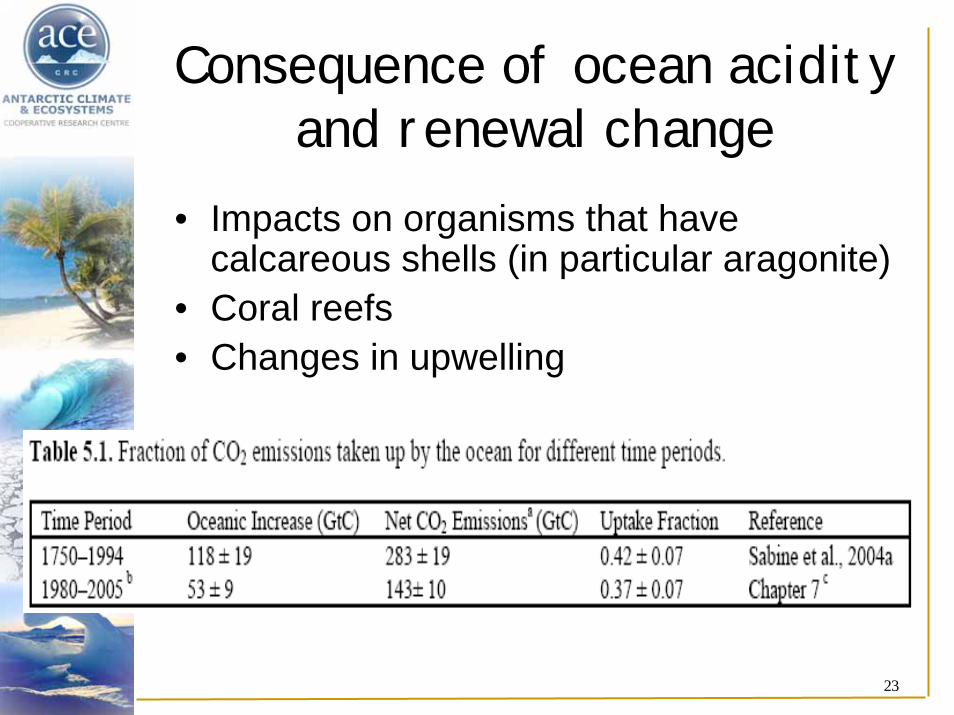
Data Distribution: profile dataOxygen

Temperatureand salinity

27

Changes on neutral surfaces

Salinity

Pot

. Tem

pera

ture

(°C

) new

ther

moc

line

old

ther

moc

line

ρ2

ρ1

Pure warming

new

ther

moc

line

old

ther

moc

line

ρ2

ρ1

Pure freshening

Salinity

Pot

. Tem

pera

ture

(°C

)

(See: Bindoff & McDougall, 1994, 2000)

28

Comparison with HADCM3

29

Comparison with CSIRO Mk3 Model

2090’s minus 1950’s

Downes et al, inprep.

30

HadCM3 1990's- 1960's

More evidence

Aoki et al, 2005

Banks and Bindoff, 2003

1960’s to 1990’s30E to 180

31

Decadal variability

31

Decadal variability

Mixed layer depths and section lines

•Bryden et al., 2003, McDonagh et al. 2005

32

1965-1987 Observed depth


1965-1987 Observed temp.


32





Observations

33

(a) (b) (c)

33

(a) (b) (c)

Zonally averaged differences on density surfaces

34

Temperature

Isopycnal depth

34

Temperature

Isopycnal depth

Time series of zonal averages at sigmat=26.7

35

Sep. 1965

Sep. 1987

35

Sep. 1965

Sep. 1987

Extremes of modelled mixed layer development

Murray et al. 2007Message: the water mass variations related Mixed layer thickness changes

36

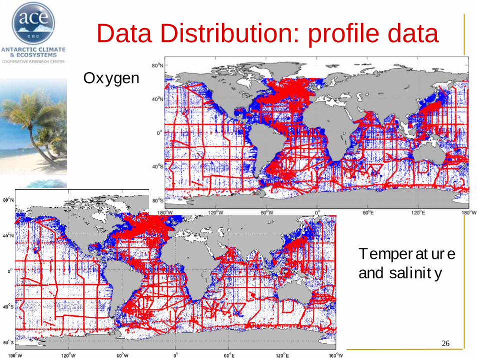
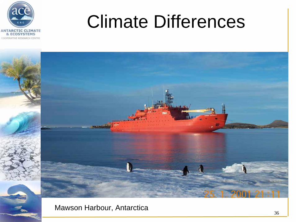
Climate Differences

Mawson Harbour, Antarctica

37

Data and method

1. Convert Hydrobase2 from pressure to density levels

2. Optimally interpolate 800,000 pre-1988 profiles to 40,000 post-1988 locations

38

Data and method

1. Convert Hydrobase2 from pressure to density levels

2. Optimally interpolate 800,000 pre-1988 profiles to 40,000 post-1988 locations

3. Directly compare 1970 with the early 1990s using a ‘snapshot’approach

Helm et al., inprep

39

Regional T-S changes

40

Salinity increases in thermocline water on isopycnals (γn=24.8)

41

Freshening of intermediate water on isopycnals (γn=27.0)

42

Zonal changes on density surfaces

Cooler/Fresher Warmer/Saltier

CDW

Mode

Salinification sub-tropics

IW

43

Deeping of isopynals in mid to high latitudes

Shoalling Deepening

CDW

Mode


IW

44

Global oxygen decreases

CDW

Mode


IW

45

Key findings 1970’s to 1990’s

• On neutral density surfaces:• Globally coherent

temperature/salinity changes• Warming/increasing salinity of upper

thermocline waters• Cooling/freshening of mode and

intermediate waters• Oxygen decrease in upper

thermocline, mode, intermediate waters and CDW

• Largest changes occurred in the

46

Summary

47

ProcessesSubduction Changes

•CSIRO Mk3 •2090’s minus 1950’s•Diagnosed using MNW•Model diagnostics

AAIW

CDW

SAMW

48

Buoyancy Changes

•CSIRO Mk3 •2090’s minus 1950’s•Diagnosed using MNW•Model diagnostics

AAIW

CDW

SAMWCW

49

Schematic of changes… CSIRO MK3 model

2090’s to 1950’s

Process that matter:

•CW Increased subduction,decreasedbuoyancy

•SAMW Decreased subduction, Decreased HF and FF

•AAIW Decreased subduction, HF and FF

•CDW Decreased entrainment, increased HF,FF

50Barnett et al. Science 2005

Parallel Climate Model

ObservationsACC Simulations

Detection

51

Implications of Climate Differences (1)

Patterns are global, coherent, consistent with earlier work.Salinity changes suggest

increased “evapouration” in sub-tropics,

increased “precipitation” at high latitudes,

and increased strength in hydrological cycle.

CDW warmed and lower in oxygenLower renewal rates, decreased ventilation (even though winds are stronger)

52

Climate Differences (Conclusions) (2)

AABW now fresher (Aoki et al, 2005)Observations are qualitatively same as climate change mode in CSIRO Mk3 model (and HadCM3)Natural variability, aliasing cannot be ignored

Heat content in 2004 and 2005

53

Thanks..

54

Comparison with HADCM3 1960-1990's

HadCM3 1990's- 1960's

55

Control HadCM3

Anthropogenicsimulation HadCM3 95%

56

Science Questions

• Global heat content of the oceans and its variations

• Global observations of oxygen change in the oceans

• Global changes in sea-level and its spatial variations

• Global observations of the cryosphere and decadal variations

57

Heat Content

Gregory et al 2004

Decadal variations

Question: why do models not simulate as much variabilityas seen in observations.

58

Oxygen Content ChangeOxygen change, WOCE- historical, 27.8 ns

Temperature change 27.8ns

Oxygen content changingon global scales- implies ocean processes are Important, is physical or Biological?

Helm et al, in prep

59

Sea-level and its spatial variations

IPCC models do not agree on spatial patterns of steric sea-level change, but do agree on SST.

Downes et al, in prep

Reasons: •Sea level is integrative•Subduction and ventilation not well simulated

Results from TAR for sea-level.

60

Cryosphere and decadal variations?

Tide-gauges

Steric Sea-level

Difference

Suggest that there is decadal variations in cryosphericcomponent to global sea-level.

Upto 78% of observed sea-level rise is from ice sheets and glaciers over the last 50 years

61

Zonal averages of ocean state

62

Shifting outcropping zones

= time1

= time2

ρ1(t1)

ρ2(t1)

ρ2(t2)

ρ1(t2)

ρ1(t1)

Shift density layer south

SOUTH NORTH

63

Global T-S profile

See Bindoff & McDougall (1994,2000)

Cooling and freshening on isopycnals may be able to be explained by ‘pure warming’

Salinity

Pot.

Tem

pera

ture

(°C

)

old

ther

moc

line

ρ2

ρ1

Pure warming

new

ther

moc

line

64

65

Revolution in ocean

observationsScientific questions:• Do we understand the heat

content record (and sea-level)?

• Do we understand the changes in ocean salinity?

• Is ocean carbon cycle changing?

• Is ocean ventilation changing?

• Can we detect the changes in the SO overturning cells.

• Assess ocean models (and GCM’s)

66

Solutions

• ACCESS evaluations– Freshening of bottom water,– Change in precipitation, carbon cycle,

heat content– Improve spatial distributions of heat,

carbon• Detection and attribution

– Natural variations or man induced?• Initialisation

67

Three underlying issues for ocean observations and models

1. Sustained observations (big risks)- operational capability (eg IMOS)- Insitu programs (ARGO, SOO, etc)

2. Timely data and model access– to ensure timely access to data so that

all may derive benefit (repository)– range of model outputs (eg ACCESS,

IPCC/PCMDI, re-analyses like BlueLINK, ECCO, SODA)

3. Need specialist Earth System Science Facility

HPC, Storage, technical support for ACCESS, and managed by/on behalf of climate scientists

68

Climate Change Initiative

• Enhanced and sustained climate measurements ($300 million over 5 years)– Ocean climate data, new ship(s),

additional support ($200 million)– Terrestrial climate networks ($100

million)

69


• An e-Research or Information Systems for Earth Systems Science ($30 million, 5 years)

• Specialist Earth Systems Science Facility (Service support and 100 Terraflops and data, ~$40million)

70


• Climate Challenge Projects ($40million)– Australia 30 year initialisation (include– Australia Re-analysis project– Australian Ocean re-analysis project

(including Southern Ocean and Antarctica)– Australian Climate Risk Managements

• New collaborative arrangements that include researchers and government

71


• Mitigation and validation service for Australian Carbon Trading Bank

72

Climate Change Initiative• Enhanced and sustained climate

measurements ($300 million over 5 years)

• e-Research or Information Systems for Earth Systems Science ($30 million, 5 years)

• Specialist Earth Systems Science Facility (Service support and 100 Terraflops and data, ~$40million, 5 years)

• Climate Challenge Projects ($30 million)• Mitigation and validation service for

Australian Carbon Trading Bank ($10 million)

• Budget ($310million)

73

91 92 93 94 95 96 97 98 99 00 01 02 03 04 05

Observational Risk – potential failures

RA/ERS-1

GFO

05 06 07 08 09 10 11 12 13 14 15 16 17 18 19

On going mission

SARALEnvisat

Approved mission GMES mission beginning development

Jason-3

Pending Jason follow-on

66°-inclination climate reference orbit

High-inclination complementary orbit

Jason-1

Sentinel 3 – 2-satellite series

Jason-2

Cryosat-2

NASA mission pending approval

SWOT

HY-2B HY-2C HY-2DHY-2A

Stan Wilson

Documents

CAWCR, ACECRC, IASOS, CSIRO University of Tasmania · PDF fileZonal changes on density ... 05 06 07 08 09 10 11 12 13 14 15 16 17 18 19 On going mission SARAL Envisat ... NASA mission