Asian Journal of Current Engineering and Maths 2: 4 July – August (2013) 260 - 266.

Contents lists available at www.innovativejournal.in

ASIAN JOURNAL OF CURRENT ENGINEERING AND MATHS

Journal homepage: http://www.innovativejournal.in/index.php/ajcem

260

CAUSALITY AND INVERTIBILITY OF AUTOREGRESSIVE INTEGRATED MOVING AVERAGE (ARIMA) MODEL

Samson Babatunde Folarin, Olaniyi Samuel Iyiola

Department of Mathematics and Statistics, King Fahd University of Petroleum and Minerals, KFUPM, Dhahran Dammam, Saudi Arabia

ARTICLE INFO

ABSTRACT

Corresponding Author Samson Babatunde Folarin Department of Mathematics and Statistics, King Fahd University of Petroleum and Minerals, KFUPM, Dhahran Dammam, Saudi Arabia Key Words: Invertibility; Causality; Stationarity; ARIMA.

In this paper, we presented causal and inverted form of Autoregressive Integrated Moving Average processes (ARIMA) of various orders, causality and invertibility conditions were established and parameters of the ARIMA (p,d,q) model were estimated using Ordinary Least Square (OLS) approach. It was deduced from the causal form of ARMA (1,q) that every is a linear combination of

and . Similarly, invertibility parameter of ARIMA

(p,d,q) is sinusoidal and . Also, converges faster to zero than .

©2013, AJCEM, All Right Reserved.

1. INTRODUCTION When fitting ARIMA model, we must check whether stationary and invertibility conditions are satisfied. All ARIMA (0, d, q) models are stationary. But we must check that they satisfy another condition, invertibility. All ARIMA (p, d, 0) models are invertible, but depending on the values of the parameters they may not be stationary. If the pure AR form of time series is of finite order, the pure MA form will be of infinite order; if the pure MA form is of finite order the pure AR is of infinite order. If both the AR and MA parts of an ARMA are of finite order, both the pure AR and the pure MA are of infinite order. Therefore while a model has various representations it makes sense to look for the simplest representations to estimate. Granger and Andersen (1978) proposed a generalized definition of invertibility and applied it to linear, non-linear and bilinear models. It was shown that some recently studied non-linear models are not invertible, but conditions for invertibility can be achieved for the other models. Anderson (1978) deduced conditions for the general Moving Average process, of order q, to be invertible or borderline non-invertible. He termed the conditions as acceptability conditions. It turned out that they depended on the magnitude of the final moving average parameter, θq. If , the process is not acceptable. Should , the conditions, for any

particular q, follow simply if use is made of the remainder theorem. When , an appeal was made to ROUCH* E'S

theorem, to establish the conditions. Analogous stationarity results immediately follow for autoregressive processes. Ojo (2009) compared subset autoregressive integrated moving average models with full autoregressive integrated moving average models. The parameters of these models were estimated and the statistical properties of the derived estimates were investigated. An algorithm was proposed to eliminate redundant parameters from the full order autoregressive integrated moving average models. In this paper, ARIMA model of various orders was presented in causal and inverted form, invertibility and causality conditions were investigated and the parameters of ARIMA were evaluated for various values of p and c at using ordinary least squares method and Crammer’s rule. 1.1 AUTOREGRESSIVE MOVING AVERAGE PROCESS The need for estimating the parameters of an ARMA (p, q) process arises in many applications both in signal processing and in automatic control. One subset of ARMA models are the so-called autoregressive, or AR models while the other is moving average or MA models. The notation ARMA (p,q) refers to the model with p autoregressive terms and q moving average terms. This model contains the AR (p) and MA (q) models

(1)

i.e (2)

The terms through are the autoregressive portion of the filter. The terms through are a

moving average of the white noise input process. 1.2 STATIONARITY OF ARMA A process is said to be strictly stationary if for any value of , the joint distribution of depends only on the interval separating the dates and not on the date (t) itself. If a

Folarin et.al/ Causality and Invertibility of Autoregressive Integrated Moving Average (ARIMA) Model

261

process is strictly stationary with finite second moments, then it must be covariance stationary (Hamilton [1994]). In short, if a time series is stationary, its mean, variance, and auto-covariance (at various lags) remain the same no matter at what point we measure them; that is, they are time invariant. ARMA process is said to be stationary if spikes decay to zero after a few lags. 1.3 SPECIFICATION OF ARMA MODELS IN TERMS OF LAG OPERATOR When the models are specified in terms of the lag operator L, the AR (p) model is given by

(3)

where

and MA (q) model is given by

(4)

where

.

ARMA (p, q) is given as

(5)

More concisely, (6)

This implies that , (7)

where

. (8)

The ARMA process is stationary if

(9)

This happens if the series converges for every Z with . Since is a rational function, the series converges for every Z with if the complex zeros of lie outside the unit circle. If we have a stationary process, then since , and the expected values of are all 0, the expected value of is also 0. An ARMA process is invertible (strictly, an invertible function of ) if there is a

(10)

with and (11)

An ARMA process is causal if there is a

(12)

with and (13)

2. ARMA Processes in Causal Form 2.1 PRESENTATION OF SOME ARMA PROCESSES IN CAUSAL FORM Here we present some ARMA process of various orders in causal form in order to provide a useful way of generating a random sequence. That is, we show a linear process as a linear combination of white noise varieties . Let . ARMA (1,1) (14)

(15)

where

(16)

ARMA (1,2) . (17)

(18)

where

Folarin et.al/ Causality and Invertibility of Autoregressive Integrated Moving Average (ARIMA) Model

262

ARMA (1,3)

(19)

(20)

where

(21)

ARMA (1,4) (22)

(23)

where

(24)

ARMA (1,q) (25)

where

(26)

This establish linear process as a linear combination of white noise variates . 2.2 INVERTIBILITY OF ARIMA MODEL OF VARIOUS ORDERS Let ARIMA (1,0,1) Recall from equation (14), that

(27)

where

(28)

ARIMA (1,1,1) (29)

(30)

where

(31)

Folarin et.al/ Causality and Invertibility of Autoregressive Integrated Moving Average (ARIMA) Model

263

This holds if . ARIMA (2,0,1) We have (32)

(33)

where

(34)

ARIMA (2,1,1) We have (35)

. (36)

where

(37)

ARMA (3,0,1) We have (38)

(39)

where

(40)

ARIMA (3, 1, 1) We have (41)

(42)

where

(43)

ARIMA (4, 0, 1) We have . (44)

Folarin et.al/ Causality and Invertibility of Autoregressive Integrated Moving Average (ARIMA) Model

264

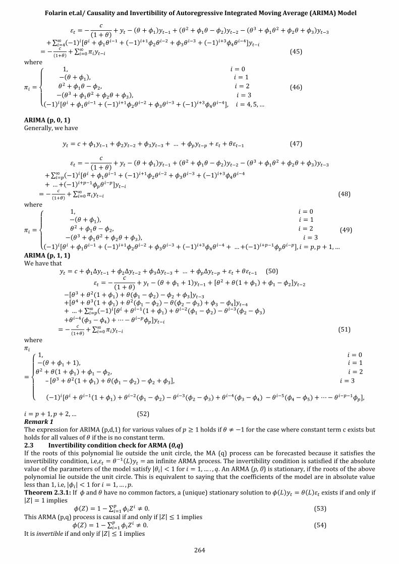
(45)

where

(46)

ARIMA (p, 0, 1) Generally, we have (47)

(48)

where

(49)

ARIMA (p, 1, 1) We have that (50)

(51)

where

(52) Remark 1 The expression for ARIMA (p,d,1) for various values of holds if for the case where constant term c exists but holds for all values of if the is no constant term. 2.3 Invertibility condition check for ARMA (0,q) If the roots of this polynomial lie outside the unit circle, the MA (q) process can be forecasted because it satisfies the invertibility condition, i.e, an infinite ARMA process. The invertibility condition is satisfied if the absolute value of the parameters of the model satisfy for . An ARMA (p, 0) is stationary, if the roots of the above polynomial lie outside the unit circle. This is equivalent to saying that the coefficients of the model are in absolute value less than 1, i.e, for . Theorem 2.3.1: If and have no common factors, a (unique) stationary solution to exists if and only if implies

(53)

This ARMA (p,q) process is causal if and only if implies

(54)

It is invertible if and only if implies

Folarin et.al/ Causality and Invertibility of Autoregressive Integrated Moving Average (ARIMA) Model

265

(55)

Theorem 2.3.2: Let be an ARMA process defined by . If for all , then there are polynomials and and a white noise sequence such that satisfies , and this is a causal, invertible ARMA process. Remark 2 Given and that ’s root is less than 1, then the process is stationary and the following also hold: 1. and have no common factors, which is not on the unit circle, so is an ARMA(1,1) process. 2. ’s root is inside the unit circle, so is not causal. 3. If the absolute value of ’s root is greater than 1(that is, outside the unit circle), so is invertible. 3 EVALUATION OF PARAMETERS OF ARIMA ( ) GIVEN THAT ARIMA (P, 0, 0) (56) Given that , we have . That is

where A is matrix and is a column matrix, that is . B is a column matrix,

. The

expression for each parameter can thus be determined using Crammer’s rule or Gauss-Schidel method.

But given that , we have , where .

ARIMA (P,1,0) (57)

When , we have . That is

When , we have

Folarin et.al/ Causality and Invertibility of Autoregressive Integrated Moving Average (ARIMA) Model

266

For the estimate of parameters in ARIMA (p,0,0) and (p,1,0), it is deduced that every term in ARIMA (p,0,0) is replaced

by in ARIMA (p,1,0). Also, is column matrix for while is ( ) column matrix for .

4 CONCLUSION In this paper, ARIMA model of various orders was presented in causal and inverted forms. Invertibility and casuality conditions were investigated. It was deduced from the causal form of ARMA (1,q), that every is a linear combination of and . Similarly for the invertibility of ARIMA (p,d,q) where and , it was deduced that is sinosidal and that . Also, converges faster to zero than as can be seen in Figure 1 below. The parameters of ARIMA were evaluated for various values of p and c at using ordinary least squares method and Crammer’s rule.

Figure1: Graph showing behaviour of for some i when and given that , , , , , , , , and . REFERENCES [1] Anderson, O.G. (1978) On the invertibility conditions for moving average processes. Statistics, vol. 9, Issue 4, 525 –

529. [2] Bobba A.G., Rudra R.P. and Diiwu J.Y. (2006) A stochastic model for identification of trends in observed hydrological

and meteorological data due to climate change in watersheds. Journal of Environmental Hydrology, Volume 14, Paper 10.

[3] Granger, C.W.J. and Andersen, A. (1978) On the invertibility of time series models. Stochastic Processes and their Applications. Volume 8, Issue 1, Pages 87-92.

[4] Gujarati, D. N. (2004) Basic Econometrics. The McGraw−Hill Companies, Fourth edition. [5] Hamilton, J. D., Time Series Analysis. Princeton University Press (1994). [6] Ion Dobre and Adriana AnaMaria Alexandru (2008) Modelling unemployment rate using Box-Jenkins Procedure.

Journal of Applied Quantitative Methods. Volume 3 No. 2 Summer. [7] Ojo J.F. (2008) Identification of optimal models in higher order of integrated autoregressive models and

autoregressive integrated moving average models in the presence of subsets. Journal of Modern Mathematics and Statistics, 2(1): 7-11.

[8] Ojo J.F. (2009) On the estimation and performance of subset autoregressive integrated moving average models. European Journal of Scientific Research. Volume 28 No 2, pp 287-293.

[9] Schwarz, G. E. (1978) Estimating the dimension of a model. Annals of Statistics 6 (2): 461–464. [10] Shittu O.I. and Yaya O.S. (2009) Measuring forecast performance of ARMA and ARFIMA; An application to US

Dollar/UK Pound foreign exchange rate. European Journal of Scientific Research, ISSN 1450-216X Volume 32 Number 2 pp. 167-176.

[11] Tuan Pham-Dinh (1978) Establishment of parameters in the ARMA, model when the characteristic polynomial of MA operator has a unit zero. Annal of Statistics, Volume 6, No. 6, 1369-1389.

[12] Umberto Triacca (2004) Feedback, causality and distance between ARMA models. Mathematics and Computers in Simulation, Volume 64, Issue 6, Pages 679-685.