Causal Dynamical Triangulation of Quantum

Gravity in Three Dimensions

J. Z. Zhang ∗

Cornell University

August 29, 2007

Abstract

The theory of causal dynamical triangulation in (2+1) dimensionsis studied through the help of Monte Carlo simulations. The basic ideasbehind this particular approach to quantum gravity are outlined in thepaper. The numerical setup and the results from the simulations arepresented and discussed. Based on the numerical results, the theory isshown to possess a non-trivial classical limit. The effective dimension ofthe emergent quantum universe is examined by means of measurementsof the fractal spectral dimension.

1 Introduction

Formulating a consistent quantum theory of gravity lies at the root of ourunderstanding of nature and still remains as one of the greatest challenges intheoretical physics today. In recent years, a particular discrete approach toquantum gravity called the causal dynamical triangulation or CDT in short,invented by Loll, Ambjorn, and Jurkiewicz, has received considerable atten-tion. The CDT approach defines quantum gravity through nonperturbativestate sums of causally triangulated geometries, and is particularly expedientfor numerical implementations. Numerical simulations in both 3 and 4 dimen-sions have yielded promising results indicating a non-trivial micro-structure ofspacetime geometry governed by quantum laws and a semi-classical behaviorof the theory in the large-scale limits [1, 2, 3]. We have developed a computer

∗jzz3@cornell.edu.

1

program to simulate the model in 3 dimensions, in hope of confirming some ofthe results obtained by Loll etc. as well as discovering other new interestinginsights for quantum gravity in 3 dimensions. In this paper, we will brieflydescribe this novel approach to quantizing gravity and discuss some of theresults we obtained in our computer simulations.

2 Quantum Gravity

Gravity in classical general relativity [4] is described by a symmetric tensorfield gµν(x) with a Lorentzian signature called the metric which determines lo-cally the values of distances and angle measurements in spacetime. The theoryis intrinsically geometric in the sense that the spacetime is represented by asmooth manifold M with measurable quantities (the metric, particle velocity,electromagnetic field, etc.) being tensor fields defined on the manifold. Thisproperty of general relativity is referred to as general covariance or diffeomor-phic invariance. The metric tensor gµν(x) satisfies the Einstein’s equationswith the energy and matter distribution in the spacetime serving as the sourceterm in these equations.

Quantum mechanics on the other hand describes the state of a physicalsystem mathematically as a vector in a Hilbert space (or a product of a setof Hilbert spaces in the case of quantum field theory). In Feynman’s pathintegral formulation of quantum mechanics [5], the quantum amplitude (innerproduct of two state vectors) of a process is given by a sum over all histories,or all possible configurations that connects the two states, each of which isweighted by e−iS, where S is the action of that history. Ordinary quantum fieldtheory describes the dynamics of elementary particles and their interactionson a fixed spacetime background, usually that of the flat Minkowski space ofspecial relativity.

Both theories work extraordinarily well at the scales for which they arevalid. However, the task of unifying the two theories under one theoreticalframework is a notoriously difficult one. The difficulties of finding a consistenttheory of quantum gravity are on the one hand due to the lack of experimentaltests and further complicated by the fact that the two theories make drasticallydifferent assumptions on how nature works. General relativity is a nonlineartheory and is thus intrinsically more complicated than linear field theories suchas electrodynamics. Moreover, the theory is nonrenormalizable so applying theusual perturbative quantum field theoretic methods fails to produce a sensibletheory of quantum gravity. General relativity is a theory of that describesthe dynamics of the geometry of spacetime, which at the same time, serves

2

as a playground for other matter fields. Therefore, quantizing gravity meansquantizing spacetime itself.

3 Causal Dynamical Triangulation

In this section, we attempt to give a rough summary of the theory of CDT.For a more thorough introduction, the read is referred to [6].

The approach of CDT follows a minimalist spirit in the sense that it isbased on a minimal set of well-known physical principles and tools such asquantum superposition, triangulation of geometry, and etc. The theory is bothbackground independent and nonperturbative, by which we mean that thetheory does not simply describe the dynamics of gravity as linear perturbationaround some preferred background metric.

To simplify the problem, we will from now on assume that we can breakup the spatial and temporal parts of our spacetime, i.e., the spacetime underconsideration has the topology [0, 1]×Σ, where Σ represents a compact spatialhypersurface. In other words, we can choose a global time function t such thateach surface of constant t is a spatial Cauchy surface.

Gravitational Path Integral

In CDT, quantization is carried out through the path integral:

G(g0,g1; t0, t1) =

∫Dg eiSEH[g] , (1)

where

SEH[g] =1

16πG

∫dnx√−g(R− 2Λ) (2)

is the usual Einstein-Hilbert action for gravitation, the variational equations ofwhich are the Einstein’s equations. Here g denotes the spacetime metric thatinterpolates between the two spatial metrics g0 and g1. General relativity istaken to be an ordinary field theory with the metric gµν representing its fielddegrees of freedom which are to be integrated over in the path integral toproduce a quantum theory.

Let us discuss briefly what it means by a gravitational path integral andaddress some related issues. Analogous to the usual interpretation of the pathintegral, the propagator G here is given by a superposition of all virtual space-times, each of which is weighted by the classical action. In contrast to the usualpath integral formulation of quantum mechanics and quantum field theory, the

3

gravitational path integral is more intricate due to the diffeomorphism invari-ance of the theory and due to the absence of a preferred background metric.Due to the diffeomorphism invariance, the path integral (1) should be takenover the space of all geometries rather than the space of all metrics becauseany two metrics are equivalent if they can be mapped onto each other by acoordinate transformation, in other words, the functional measure Dg must bedefined in a covariant way. Because there is no obvious way to parametrize ge-ometries, one may suggest that we introduce covariant metric tensor as a fieldvariable to evaluate the integral. However, this leads to the complication thatgauge fixing the metric tensor using techniques such as the Faddeev-Popovdeterminants requires exceedingly difficult nonperturbative evaluation.

The path integral as it stands is not mathematically well-defined. In or-dinary quantum field theory, to actually evaluate the integral one usuallyperforms a Wick rotation by analytically continuing the time variable t tothe imaginary axis, i.e., t 7→ it. The Wick rotation converts a problem inLorentzian spacetime MLor to one in Euclidean space MEuc. It is not obvioushow the Wick rotation needs to be carried out in the gravitational setting.The ad hoc substitution iSLor → −SEuc that is used widely in field theories isin fact the basis for the predecessor of CDT, the Euclidean dynamical trian-gulation [7]. As will be discussed shortly, CDT is based on a different programfor carrying out the Wick rotation, one that specifically preserves the causalityof spacetime, setting it apart from the old Euclidean approach.

Regge Calculus

To perform the calculation nonperturbatively, we use a lattice method similarto those used in lattice gauge theories. In the field theoretic context, the latticespacing a will naturally serve as a cutoff of the theory. The continuum limit isextracted by taking the lattice spacing a to zero and hoping that the resultingtheory is independent of the cutoff. This suggests that we need some specificscheme for discretization of spacetime geometries. The idea of approximatinga spacetime manifold by a piecewise flat spacetime was first developed byRegge [8] and is called the Regge calculus which has been successfully appliedin numerical general relativity and quantum gravity before CDT [9].

Instead of considering spaces with smooth curvature, Regge looked atspaces where the curvature is restricted to subspaces of codimension two, basedon the division of the manifold into elementary building blocks which are usu-ally taken to be simplices, i.e., higher dimensional analogs of triangles, withconsistent edge length assignments li. For example, a simplex in two dimen-sions is a flat triangle and in three dimensions a tetrahedron, and so on. A

4

simplicial manifold or equivalently a triangulation of a smooth manifold is ob-tained by gluing together these simplicial building blocks in an appropriatemanner. The Einstein-Hilbert action can then be written as a functional ofthe edge lengths only, by making the following substitutions [10]:∫

dnx√−gR → 2

∑j∈T

εj , (3)

∫dnx√−g →

∑j∈T

Vj , (4)

where j is an index labeling the hinges, i.e., the elements of codimension two(points in 2D, edges in 3D, triangular faces in 4D, and etc.) where curvatureresides in a particular triangulation T . εj is the so-called deficit angle andVj the dual volume of the hinge j. In terms of these geometric variables, theaction (2) is written as

SRegge({l2i }) =∑j∈T

(k εj − Vj λ) , (5)

where k ≡ 1/8πG is the inverse Newton’s constant and λ ≡ kΛ/2 is theredefined cosmological constant.

Dynamical Triangulation

Since in Regge calculus each triangulation T is completely characterized bythe set of all squared edge lengths {l2i }, we can in principle carry out thepath integral by integrating over all possible edge lengths, i.e.,

∫Dg →

∫Dl,

with each configuration {l2i } weighted by the corresponding Regge action (5).However, a problem with this approach is that certain triangulations may beover counted due to the gauge freedom in the edge lengths since each edgelength is varied continuously. Moreover, one would still like to introduce asuitable cut-off scale for the edge length. Instead, a more restricted version ofRegge calculus called dynamical triangulation is employed in CDT.

In dynamical triangulation, one again uses simplicial manifolds and theRegge form of the action, but a different space of triangulated geometries inthe path integral. Instead of integrating over all possible edge lengths for afixed simplicial manifold, one fixed the lengths of the basic simplicial buildingblocks, and sums over all distinct triangulations of M . It is to be noted thatfixing the edge lengths is not a restriction on the metric degrees of freedomsince one can still achieve all kinds of deficit angles by appropriate gluing of the

5

t

x

t1

t0

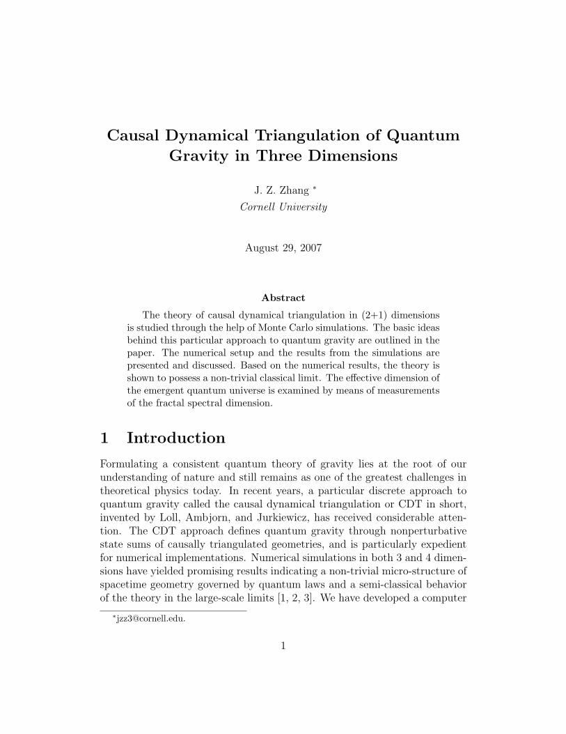
(3,1) (2,2) (1,3)

Figure 1: The three types of basic building blocks in three dimensions.

simplicial building blocks. The continuum path integral can thus be writtenas a discrete sum over inequivalent dynamical triangulations:∫

Dg eiSEH[g] →∑T∈T

1

C(T )eiSRegge(T ) , (6)

where 1/C(T ) is the measure on the space of triangulations, with C(T ) beingthe order of the automorphism group of the triangulation T . From a numericalpoint of view, this is extremely convenient since information about the geom-etry is reduced to combinatorics, in other words, geometric quantities suchas volume and curvature can be obtained by simple counting of the simplicialelements (points, edges, faces, etc.). In addition, an approximation of the pathintegral can be obtained numerically by sampling the configuration space ofall dynamical triangulations (discrete metrics) T . This is exactly what we doin our computer simulations which will be described in detail in section 4.

Role of Causality

Now we are left with the question of how to perform a Wick rotation and ex-plicitly compute the sum in (6). In the old Euclidean dynamical triangulationapproach, one makes the substitution iSLor → −SEuc and sum over the Eu-clidean counterparts of the dynamically triangulated Lorentzian geometries,i.e., discrete geometries made up of Euclidean simplicial building blocks. Theproblem with the Euclidean approach is that the Euclidean geometries thatconstitute the path integral know nothing about causality, namely the light-cone structure of the spacetime and there is no a priori prescription of how to

6

t

x

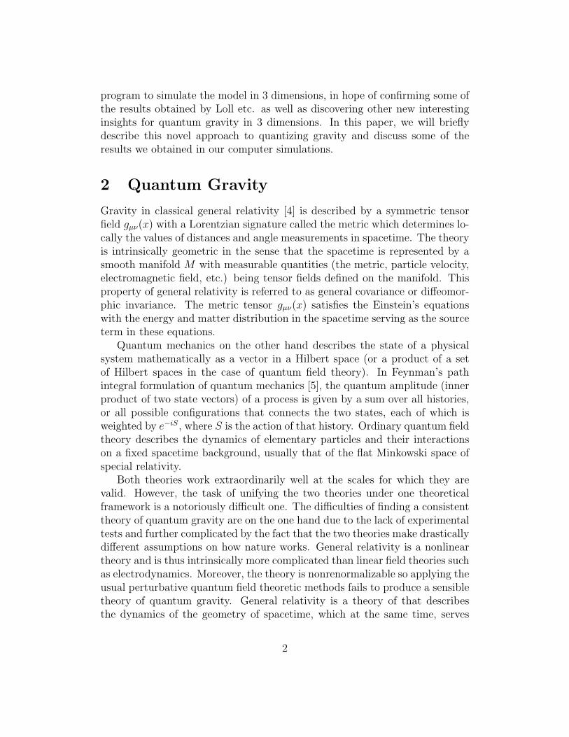
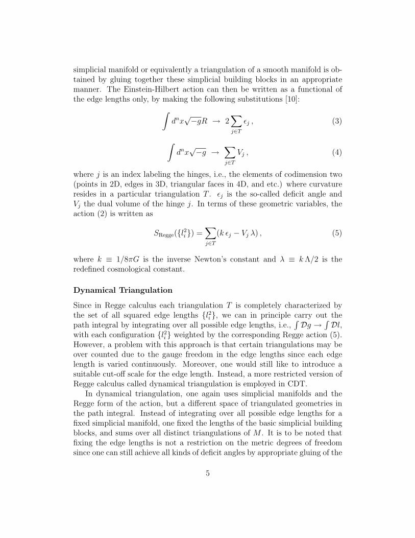
Figure 2: A local subset of a causal dynamical triangulation in three dimensions.Note that each building block tetrahedron has the inherent light-cone structure ofa Minkowski space

perform an inverse Wick rotation to recover causality in the full quantum the-ory. Furthermore, due to the absence of time a large class of highly degenerategeometries contributes to the path integral, causing a well-defined continuumtheory fails to exist.

On the contrary, in CDT the causal structure is built into the discretegeometries from the outset. The geometries that are summed over are takento be the same homeomorphism class, i.e., we do not allow different spacetimetopologies to contribute to the path integral. As mentioned before, we will onlyconsider globally hyperbolic simplicial manifolds with a time-foliated structure,where the (n − 1)-dimensional spatial slices (each labeled by the global timet, not a gauge choice) have a fixed topology (usually taken to be Sn−1). Inother words, topology changes of the spatial slices are not allowed becausespatial topology changes are often associated with causality violation. Eachsimplicial building block in CDT is taken to be a subset of the Minkowskispace together with its inherent light-cone structure. Again, a triangulatedgeometry along with its global causal structure is obtained by suitable gluingof these simplicial building blocks, each of which has its own local causality,whose spacelike edges all have the same length squared a2 and whose timelikeedges all have the same length squared −αa2, where α denotes an asymmetryfactor between the spacelike and timelike geodesic distances. This leaves us

7

with n types of simplicial building blocks in n dimensions. The three typesof building blocks in 3 dimensions are shown in Figure 1. An example of howthey are glued together to form a local subset of a 3-dimensional simplicialspacetime is shown in Figure 2.

Wick Rotation and the Euclidean Action

In CDT, Wick rotation is defined by analytical continuation of all timelikeedges of each simplicial building block respectively to the Euclidean sector, i.e.,by making the substitution −αa2 → αa2 for the length square of the timelikeedges. This takes a discrete Lorentzian geometry TLor to its correspondingEuclidean geometry TEuc. As a result, the Lorentzian action is replaced by thecorresponding Euclidean action1, i.e.,

iSLor ≡ iSRegge(TLor) → −SEuc ≡ iSRegge(TEuc) (7)

The Wick rotation in effect converts a path integral (a quantum mechan-ical problem) to a partition function (a statistical mechanical problem). Theconfiguration space of dynamically triangulated spacetimes T after the Wickrotation can be viewed as a statistical ensemble with the partition function

Z =∑T∈T

e−SE(T ) , (8)

where SE(T ) is the Euclidean Regge action of the triangulation T . Here wehave taken the measure factor 1/C(T ) to be 1 simply because that based onthe general observation in the theory of critical phenomena we do not expectthe detailed choice of the measure to affect the continuum limit of the theory.This assumption is further supported by the analytical solution to the CDTmodel in two dimensions [12]. After rewriting the problem in the languageof statistical mechanics, we can readily employ the Monte Carlo method totackle the problem with computer simulations.

4 Numerical Implementation in 3D

In this section and the rest of the paper, we will only consider the CDT modelin three dimensions. Gravity in three dimensions often provides a simplersetting for quantization [13]. For instance, classical 3D gravity is devoid ofpropagating degrees of freedom. The lower-dimensional theory can serve asan interesting toy model for the study of quantum gravity. In this section, wedescribe the numerical setup of our simulation.

1The derivation of this can be found in [11]

8

Partition Function

It can be shown that in three dimensions and for the special case α = −1 (sym-metric timelike and spacelike discrete geodesic lengths) the discrete Euclideanaction is expressible in terms of the total number of vertices and tetrahedra,N0 and N3, in the triangulation T , and takes the form [1]

SE(T ) = −k0N0 + k3N3 , (9)

where

k0 =a

4G

k3 =a3Λ

48√

2πG+

a

4G

(3

πarccos

1

3− 1

).

(10)

The dimensionless coupling constants k0 and k3 will simply be referred toas the inverse Newton’s constant and the cosmological constant, respectively.The partition function (8) can thus be written as

Z(k0, k3) =∑T∈T

ek0N0−k3N3 . (11)

One can show that, for finite volume, the model described above is well-definedin the sense of being a statistical system whose transfer matrix is bounded andpositive [11].

Data Structure

The particular time-foliated structure of the simplicial manifolds under consid-eration allows a discretization of the global proper time t. In our simulations,the total number of time intervals is taken to be 8, 16, 32, and 80. For exam-ple, in a triangulation with 16 time intervals, each spatial slice is labeled by anintegral number between 0 and 16. On the other hand, since each 3-simplex(tetrahedron) sits between two spatial slices, it is labeled with a half-integer.

As already mentioned in the previous section, there are only three types ofbasic building blocks in three dimensions (Figure 1). We denote each of thesebuilding blocks by the number of points it has in the adjacent spatial slices.For instance, the (1,3) simplex has 1 vertex point at t and 3 vertex points att + 1, and so on. The number of (1,3) simplices in the time interval [t, t + 1]will be denoted by N13(t), and likewise for the (2,2) and (3,1) simplices. Thefollowing list summarizes the notation we will adopt throughout the remainingpaper.

9

N0 - number of 0-simplices (points)N1 - number of 1-simplices (edges)N2 - number of 2-simplices (triangles)N3 - number of 3-simplices (tetrahedra)N13 - number of (1,3) simplicesN22 - number of (2,2) simplicesN31 - number of (3,1) simplices

Since each triangulated spacetime consists of a set of tetrahedra glued toeach other in a specific manner, the data structure we need to deal with inour computer program is not particularly complicated. We use a hash tableto store the current configuration during the simulation. Each point in theconfiguration is labeled by a natural number. In addition, every tetrahedronis assigned an id number which points to a particular entry in the hash table.Each entry in the hash table is a list of numbers that represents the propertiesof the corresponding tetrahedron. Each list has the structure

(y, t, p1, p2, p3, p4, n1, n2, n3, n4) , (12)

where y represents the type of the tetrahedron and takes the values 1, 2 or3 for (1,3), (2,2), or (3,1) simplices, respectively, t is the time at which thetetrahedron resides and assumes half-integer values, the numbers p1 through p4

are the labels of the four vertex points, and n1 through n4 are the id numbersof the four neighboring tetrahedra that are glued to this tetrahedron (sharingexactly three points). We order the vertex points in the way such that pointsat the earlier time are placed before the points at the latter time. In addition,the neighboring tetrahedron ni is glued to the face that does not contain thepoint pi. For example, the list (3, 1

2, 1, 2, 3, 4, 10, 11, 12, 13) represents a (3,1)

simplex at t = 1/2 having the vertex points 1, 2, 3, and 4 and are connectedto the tetrahedra with id numbers 10, 11, 12, and 13. It can also be inferredfrom the list that the points 1, 2, and 3 are anchored at t = 0 while the point4 at t = 1 as well as the fact that the neighboring tetrahedron 10 shares thetriangle 234, and so on.

Monte Carlo Moves

Starting from any initial configuration, the Monte Carlo method generatesrandom configurations by a random walk through the configuration space (inour case, T ). Using the technique of detailed balance, we will be able tocalculate the expectation value of any observable. Each step in the random

10

walk is usually referred to as a Monte Carlo move. The computer simulationrandomly generates successive Monte Carlo moves and modifies the hash tableaccording to the rules associated with each of the moves.

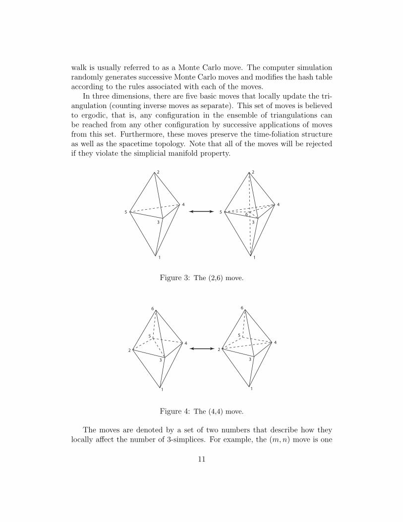
In three dimensions, there are five basic moves that locally update the tri-angulation (counting inverse moves as separate). This set of moves is believedto ergodic, that is, any configuration in the ensemble of triangulations canbe reached from any other configuration by successive applications of movesfrom this set. Furthermore, these moves preserve the time-foliation structureas well as the spacetime topology. Note that all of the moves will be rejectedif they violate the simplicial manifold property.

2

5

1

4

3

2

5

1

4

3

6

Figure 3: The (2,6) move.

6

2

5

4

3

1

6

2

5

4

3

1

Figure 4: The (4,4) move.

The moves are denoted by a set of two numbers that describe how theylocally affect the number of 3-simplices. For example, the (m,n) move is one

11

4 2

1

3

5

4 2

1

3

5

Figure 5: The (2,3) move.

that operates on a local subset ofm tetrahedra and replaces it by one consistingof n tetrahedra. These moves are illustrated in Figure 3, 4, and 5 where we havealso shown the labels of the vertices of the initial and resulting simplices. Forinstance, the (2,3) move acts on a subset that consists of a (3,1) simplex and a(2,2) simplex sharing one triangular face and turn it into a subset consisting ofa (3,1) simplex together with the two other (2,2) simplices. The correspondinginverse move, the (3,2) move, does the exact opposite. Note that the time-reversed version of the above move is also valid. To illustrate explicitly how themoves change the hash table where the information about the triangulation isstored, we show how the lists of a local subset of tetrahedra (with id numbers1 and 2) are modified by the (2,3) move for the case illustrated in Figure 5:

1 : (3,1

2, 1, 3, 5, 4, 2, 0, 0, 0)

2 : (2,1

2, 3, 5, 4, 2, 0, 0, 0, 1)

⇓

3 : (3,1

2, 1, 3, 5, 2, 0, 5, 2, 0)

4 : (2,1

2, 1, 3, 4, 2, 0, 5, 3, 0)

5 : (2,1

2, 1, 5, 2, 4, 0, 4, 0, 3)

(13)

Here 0 simply indicates that the tetrahedron is not connected to any other atthat face. A more detailed description of these moves can be found in [11].

Metropolis Algorithm

In order to get sensible, accurate results when simulating statistical systemswith a rapidly varying Boltzmann weight (e−SE in our case), it is vital to use theidea of importance sampling in Monte Carlo integration. The ideal situation is

12

to sample configurations with a probability given by their Boltzmann weight.Then the Monte Carlo average of N measurements of an observable A wouldjust be

〈A〉 ≡∑

T∈T A(T )e−SE(T )

Z≈ 1

N

N∑i

A(Ci) , (14)

where Ci is the so-called Markov chain of configurations sampled during thesimulation. To set up the Markov chain we need to introduce a fictitiousdynamics by adjusting the probability of making a transition from one config-uration to another based on the change in the Boltzmann weight.

Let P (Ci) be the probability of being in configuration Ci and W (Ci, Ci+1)be the transition probability of going from Ci to Ci+1. The so-called detailedbalance condition assures that the random walk reaches an equilibrium prob-ability distribution and is expressed as

W (Ci, Ci+1)P (Ci) = W (Ci+1, Ci)P (Ci+1) . (15)

In terms of the current problem of the statistics of triangulated geometries,the condition is written as

W (T1, T2)

W (T2, T1)=P (T2)

P (T1)=e−SE(T2)

e−SE(T1)= e−∆SE . (16)

The simplest choice of W that satisfies the detailed balance condition is givenby

W (T1, T2) =

{e−∆SE if ∆SE > 0

1 if ∆SE ≤ 0. (17)

This dynamic method of generating an arbitrary probability distribution isusually referred to as the Metropolis algorithm [14]. According to this condi-tion, each Monte Carlo move is accepted or rejected based on the change inthe Euclidean action.

Technical Details of Simulation

In all of our simulations, the spacetime topology is fixed to be S1× S2, wherethe periodic identification in the time direction has been chosen purely forpractical convenience2. The strategy for the simulation is the usual one fromdynamical triangulations. We first need to fine-tune the bare cosmological

2We have in fact run our simulation with other boundary conditions. The results haveshown be to largely independent of the boundary condition specified.

13

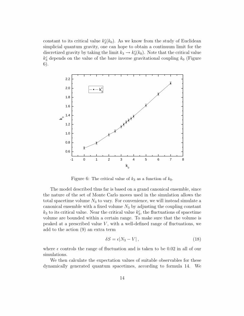
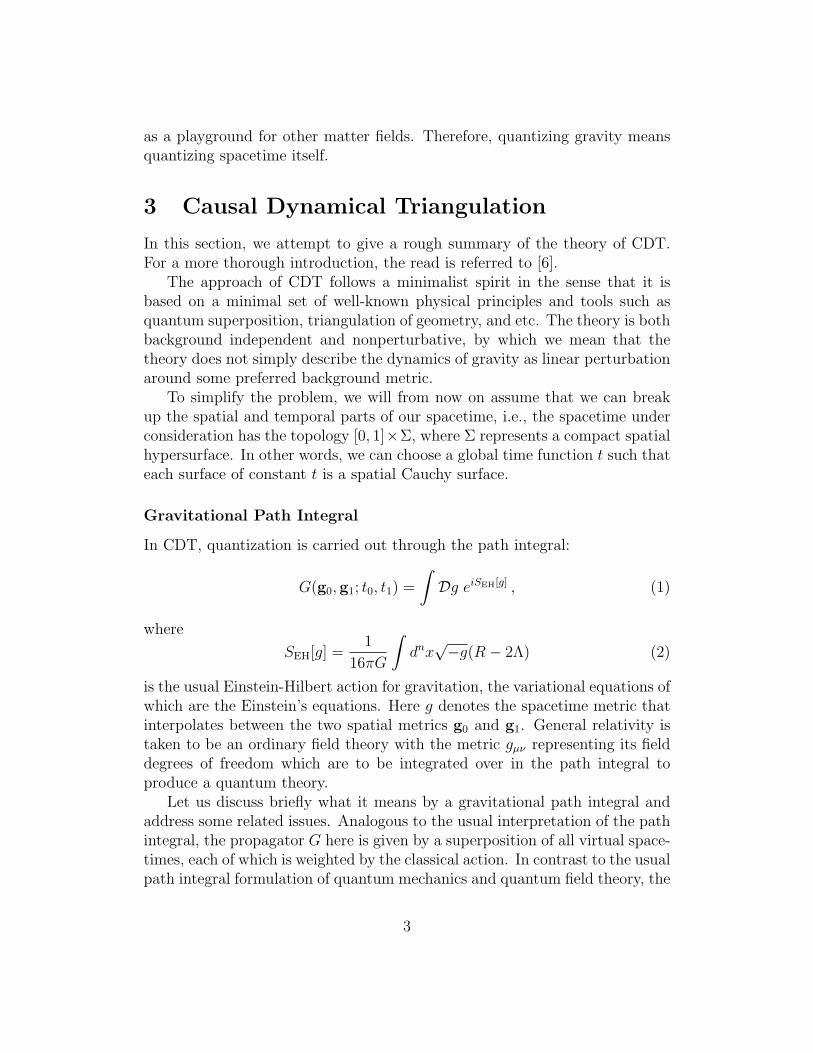
constant to its critical value kc3(k0). As we know from the study of Euclideansimplicial quantum gravity, one can hope to obtain a continuum limit for thediscretized gravity by taking the limit k3 → kc3(k0). Note that the critical valuekc3 depends on the value of the bare inverse gravitational coupling k0 (Figure6).

- 1 0 1 2 3 4 5 6 7 80 . 6

0 . 8

1 . 0

1 . 2

1 . 4

1 . 6

1 . 8

2 . 0

2 . 2

k 3

k 0

k c3

Figure 6: The critical value of k3 as a function of k0.

The model described thus far is based on a grand canonical ensemble, sincethe nature of the set of Monte Carlo moves used in the simulation allows thetotal spacetime volume N3 to vary. For convenience, we will instead simulate acanonical ensemble with a fixed volume N3 by adjusting the coupling constantk3 to its critical value. Near the critical value kc3, the fluctuations of spacetimevolume are bounded within a certain range. To make sure that the volume ispeaked at a prescribed value V , with a well-defined range of fluctuations, weadd to the action (9) an extra term

δS = ε|N3 − V | , (18)

where ε controls the range of fluctuation and is taken to be 0.02 in all of oursimulations.

We then calculate the expectation values of suitable observables for thesedynamically generated quantum spacetimes, according to formula 14. We

14

1 2 3 4 5 6- 0 . 0 5

0 . 0 0

0 . 0 5

0 . 1 0

0 . 1 5

0 . 2 0

0 . 2 5

0 . 3 0

0 . 3 5

0 . 4 0 T = 8 V = 8 k T = 3 2 V = 3 2 k

<N22

/N 3>

k 0

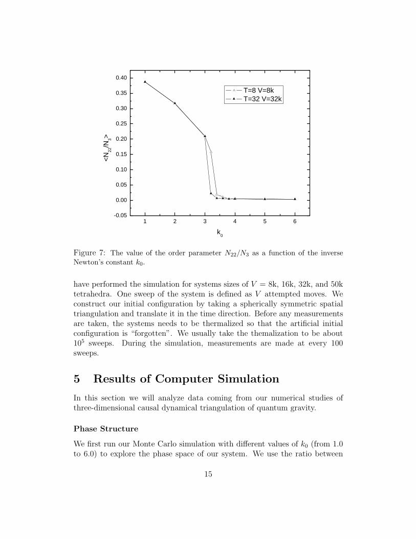
Figure 7: The value of the order parameter N22/N3 as a function of the inverseNewton’s constant k0.

have performed the simulation for systems sizes of V = 8k, 16k, 32k, and 50ktetrahedra. One sweep of the system is defined as V attempted moves. Weconstruct our initial configuration by taking a spherically symmetric spatialtriangulation and translate it in the time direction. Before any measurementsare taken, the systems needs to be thermalized so that the artificial initialconfiguration is “forgotten”. We usually take the themalization to be about105 sweeps. During the simulation, measurements are made at every 100sweeps.

5 Results of Computer Simulation

In this section we will analyze data coming from our numerical studies ofthree-dimensional causal dynamical triangulation of quantum gravity.

Phase Structure

We first run our Monte Carlo simulation with different values of k0 (from 1.0to 6.0) to explore the phase space of our system. We use the ratio between

15

the total number of (2,2) simplices N22 and the total spacetime volume N3 asan order parameter. Figure 7 shows the expectation value of the ratio N22/N3

as a function of the coupling constant k0 for two different types of spacetimeconfiguration. We observe a phase transition at the critical value kc

0 of about3.3.

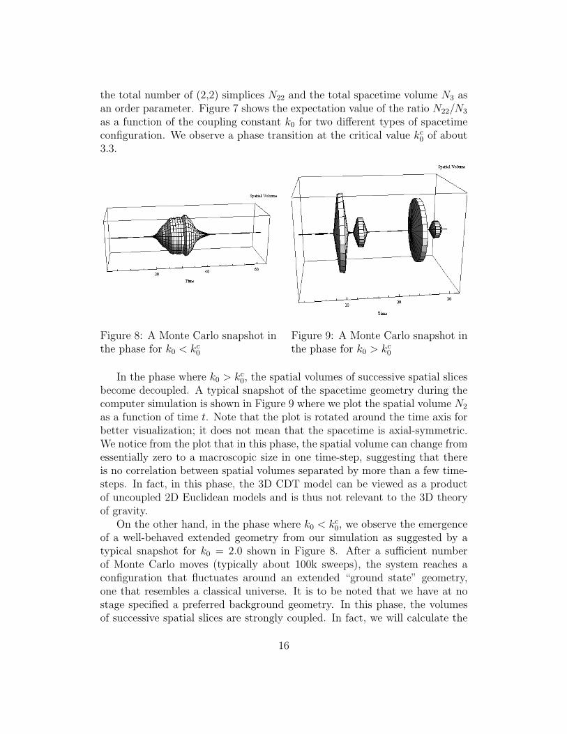
Figure 8: A Monte Carlo snapshot inthe phase for k0 < kc0

Figure 9: A Monte Carlo snapshot inthe phase for k0 > kc0

In the phase where k0 > kc0, the spatial volumes of successive spatial slices

become decoupled. A typical snapshot of the spacetime geometry during thecomputer simulation is shown in Figure 9 where we plot the spatial volume N2

as a function of time t. Note that the plot is rotated around the time axis forbetter visualization; it does not mean that the spacetime is axial-symmetric.We notice from the plot that in this phase, the spatial volume can change fromessentially zero to a macroscopic size in one time-step, suggesting that thereis no correlation between spatial volumes separated by more than a few time-steps. In fact, in this phase, the 3D CDT model can be viewed as a productof uncoupled 2D Euclidean models and is thus not relevant to the 3D theoryof gravity.

On the other hand, in the phase where k0 < kc0, we observe the emergence

of a well-behaved extended geometry from our simulation as suggested by atypical snapshot for k0 = 2.0 shown in Figure 8. After a sufficient numberof Monte Carlo moves (typically about 100k sweeps), the system reaches aconfiguration that fluctuates around an extended “ground state” geometry,one that resembles a classical universe. It is to be noted that we have at nostage specified a preferred background geometry. In this phase, the volumesof successive spatial slices are strongly coupled. In fact, we will calculate the

16

Ra

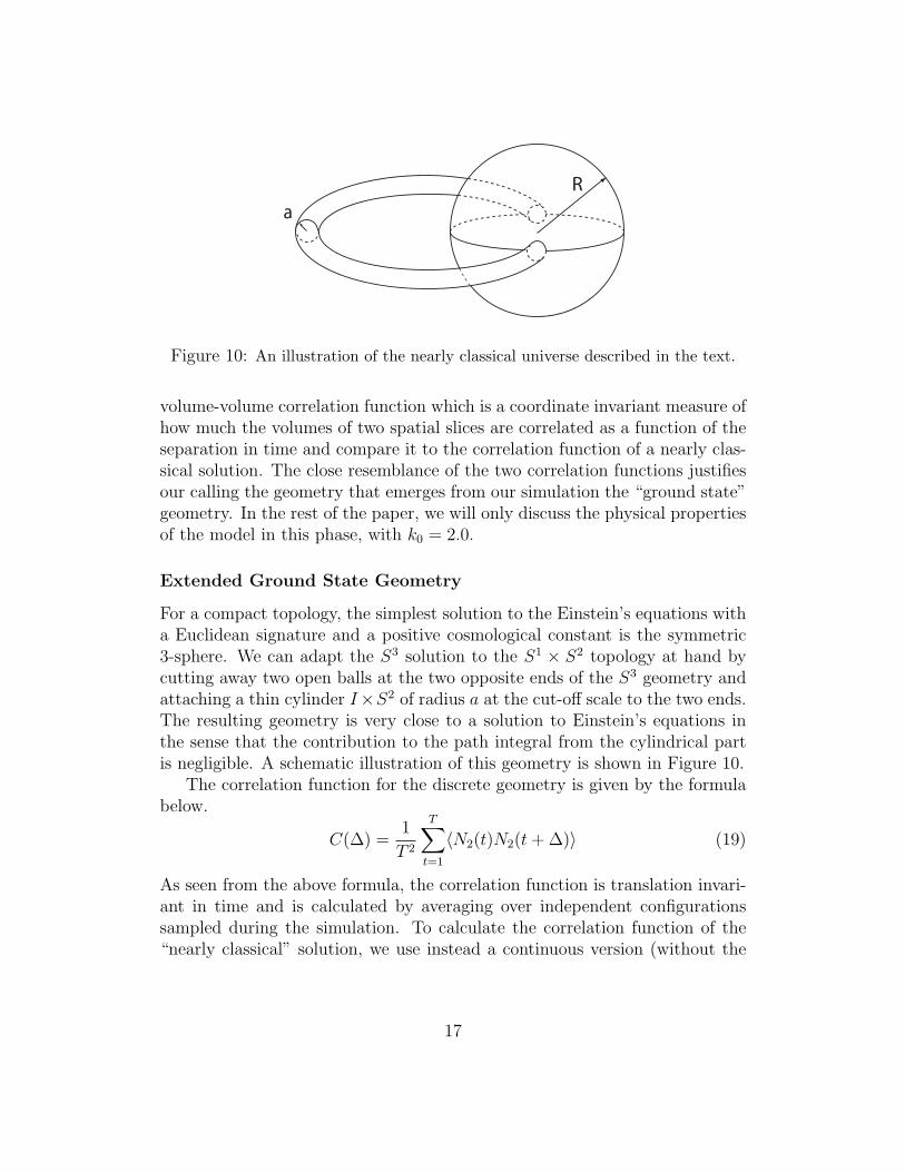
Figure 10: An illustration of the nearly classical universe described in the text.

volume-volume correlation function which is a coordinate invariant measure ofhow much the volumes of two spatial slices are correlated as a function of theseparation in time and compare it to the correlation function of a nearly clas-sical solution. The close resemblance of the two correlation functions justifiesour calling the geometry that emerges from our simulation the “ground state”geometry. In the rest of the paper, we will only discuss the physical propertiesof the model in this phase, with k0 = 2.0.

Extended Ground State Geometry

For a compact topology, the simplest solution to the Einstein’s equations witha Euclidean signature and a positive cosmological constant is the symmetric3-sphere. We can adapt the S3 solution to the S1 × S2 topology at hand bycutting away two open balls at the two opposite ends of the S3 geometry andattaching a thin cylinder I×S2 of radius a at the cut-off scale to the two ends.The resulting geometry is very close to a solution to Einstein’s equations inthe sense that the contribution to the path integral from the cylindrical partis negligible. A schematic illustration of this geometry is shown in Figure 10.

The correlation function for the discrete geometry is given by the formulabelow.

C(∆) =1

T 2

T∑t=1

〈N2(t)N2(t+ ∆)〉 (19)

As seen from the above formula, the correlation function is translation invari-ant in time and is calculated by averaging over independent configurationssampled during the simulation. To calculate the correlation function of the“nearly classical” solution, we use instead a continuous version (without the

17

- 4 0 - 2 0 0 2 0 4 0

0 . 0

0 . 5

1 . 0

1 . 5

2 . 0

2 . 5

T = 8 0 V = 5 0 k " C l a s s i c a l U n i v e r s e "

C(∆)

∆

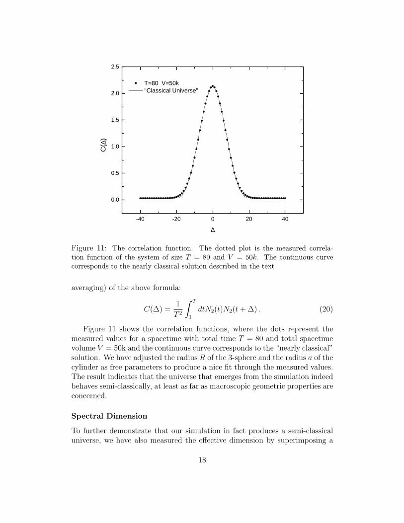
Figure 11: The correlation function. The dotted plot is the measured correla-tion function of the system of size T = 80 and V = 50k. The continuous curvecorresponds to the nearly classical solution described in the text

averaging) of the above formula:

C(∆) =1

T 2

∫ T

1

dtN2(t)N2(t+ ∆) . (20)

Figure 11 shows the correlation functions, where the dots represent themeasured values for a spacetime with total time T = 80 and total spacetimevolume V = 50k and the continuous curve corresponds to the “nearly classical”solution. We have adjusted the radius R of the 3-sphere and the radius a of thecylinder as free parameters to produce a nice fit through the measured values.The result indicates that the universe that emerges from the simulation indeedbehaves semi-classically, at least as far as macroscopic geometric properties areconcerned.

Spectral Dimension

To further demonstrate that our simulation in fact produces a semi-classicaluniverse, we have also measured the effective dimension by superimposing a

18

diffusion process on the discretized geometric ensemble. The method is de-scribed in detail in [15]. The basic idea is to perform a random walk in agiven spacetime configuration after the Monte Carlo simulation has thermal-ized. Starting from any tetrahedron, a random path is generated by randomlywalking to one of the four neighboring tetrahedra at each successive step.From a large number of random paths of σ steps, one can extrapolate thereturn probability P (σ), namely the probability of a random walk that startsand ends at the same tetrahedron in σ steps. Since we are interested in theregion of spacetime with extended spatial volume, we will only start the ran-dom walks on the spatial slice with the maximal spatial volume. Moreover,we average over the return probabilities obtained with different starting tetra-hedra and on independent spacetime configurations generated in the MonteCarlo simulation.

The return probability for diffusion on fractal geometry is well-studied andis given by the formula

P (σ) ≈ σ−D/2 , (21)

when the diffusion time is considerably smaller than N2/D3 . Here D is the

so-called spectral dimension, which is not necessarily an integer. The spec-tral dimension can be extracted from the return probability by taking thelogarithmic derivative if the finite-size correction is neglected, i.e.,

D(σ) = −2d logP (σ)

d log σ+ finite-size correction. (22)

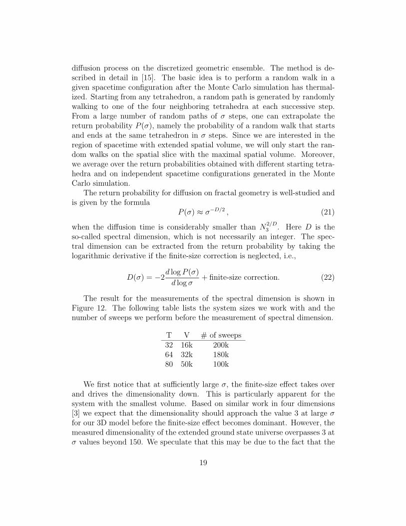
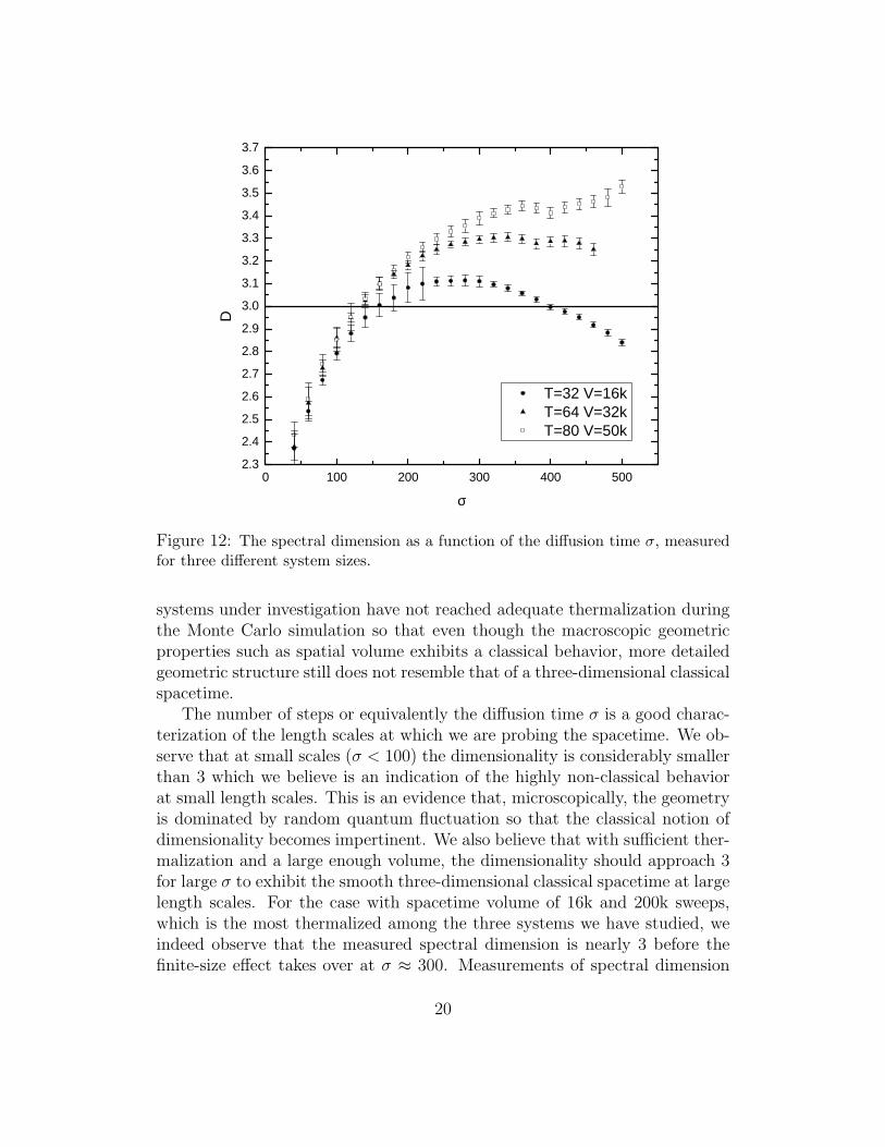
The result for the measurements of the spectral dimension is shown inFigure 12. The following table lists the system sizes we work with and thenumber of sweeps we perform before the measurement of spectral dimension.

T V # of sweeps32 16k 200k64 32k 180k80 50k 100k

We first notice that at sufficiently large σ, the finite-size effect takes overand drives the dimensionality down. This is particularly apparent for thesystem with the smallest volume. Based on similar work in four dimensions[3] we expect that the dimensionality should approach the value 3 at large σfor our 3D model before the finite-size effect becomes dominant. However, themeasured dimensionality of the extended ground state universe overpasses 3 atσ values beyond 150. We speculate that this may be due to the fact that the

19

0 1 0 0 2 0 0 3 0 0 4 0 0 5 0 02 . 32 . 42 . 52 . 62 . 72 . 82 . 93 . 03 . 13 . 23 . 33 . 43 . 53 . 63 . 7

T = 3 2 V = 1 6 k T = 6 4 V = 3 2 k T = 8 0 V = 5 0 k

D

σ

Figure 12: The spectral dimension as a function of the diffusion time σ, measuredfor three different system sizes.

systems under investigation have not reached adequate thermalization duringthe Monte Carlo simulation so that even though the macroscopic geometricproperties such as spatial volume exhibits a classical behavior, more detailedgeometric structure still does not resemble that of a three-dimensional classicalspacetime.

The number of steps or equivalently the diffusion time σ is a good charac-terization of the length scales at which we are probing the spacetime. We ob-serve that at small scales (σ < 100) the dimensionality is considerably smallerthan 3 which we believe is an indication of the highly non-classical behaviorat small length scales. This is an evidence that, microscopically, the geometryis dominated by random quantum fluctuation so that the classical notion ofdimensionality becomes impertinent. We also believe that with sufficient ther-malization and a large enough volume, the dimensionality should approach 3for large σ to exhibit the smooth three-dimensional classical spacetime at largelength scales. For the case with spacetime volume of 16k and 200k sweeps,which is the most thermalized among the three systems we have studied, weindeed observe that the measured spectral dimension is nearly 3 before thefinite-size effect takes over at σ ≈ 300. Measurements of spectral dimension

20

on more thermalized systems are currently in progress. There is hope that amore accurate measurement will yield the result that the dimensionality ap-proaches the value 3 asymptotically for increasing σ and will also allow us toextrapolate the behavior of the dimensionality in the limit as σ → 0.

6 Conclusion

In sum, our numerical simulation of the three-dimensional CDT model hasproduced results in agreement with the results obtained by Loll, and etc.A well-behaved extended ground state universe emerges dynamically in theMonte Carlo simulation. For the first time, measurements of the spectraldimension of the emergent universe are conducted on a 3D CDT model. Ascale dependence of the spectral dimension is also observed. A more precisemeasurement of the spectral dimension will hopefully yield more persuasiveresults for the behavior of the dimensionality in the limit of large and smalllength scales.

This project provides a basis for further work on CDT in three dimensions.There are a number of generalizations to the model that are interesting tostudy. In our simulations, we have restricted the spatial topology to be thatof S2. In the future, we can adapt the model to spaces of torus topologyand compare the results to analytical solutions based on other approaches toquantum gravity. We can also examine the effects of matter fields (ex. a scalarboson φ) coupled to gravity.

7 Acknowledgments

The author would like to thank his collaborator Rajesh Kommu and his advisorProfessor Steve Carlip, both of physics department at UC Davis, for helpfulguidance on this project. The work is supported by the NSF REU programat UC Davis.

References

[1] J. Ambjørn, J. Jurkiewicz and R. Loll, Non-perturbative 3d Lorentzianquantum gravity, Phys. Rev. D 64 044011, (2001), [arXiv:hep-th/0105267].

21

[2] J. Ambjørn, J. Jurkiewicz and R. Loll, Emergence of a 4D world fromcausal quantum gravity, Phys. Rev. Lett. 93 (2004) 131301 [arXiv:hep-th/0404156].

[3] J. Ambjørn, J. Jurkiewicz and R. Loll, Spectral dimension of the universe,Phys. Rev. Lett. 95 (2005) 171301 [arXiv:hep-th/0505113].

[4] R. M. Wald, General Relativity, (The University of Chicago Press, 1984).

[5] R. P. Feynman and A. R. Hibbs, Quantum Physics and Path Integrals,(McGraw-Hill, 1965).

[6] J. Ambjørn, J. Jurkiewicz and R. Loll, The universe from scratch, Con-temp. Phys. 47 (2006) 103-117 [arXiv:hep-th/0509010].

[7] J. Ambjørn and J. Jurkiewicz, Four-dimensional simplicial quantum grav-ity, Physics Letters B 278 42-50, (1992).

[8] T. Regge, General relativity without coordinates, Nuovo Cim. 19: 558-571,(1961).

[9] R. M. Williams and P. A. Tuckey, Regge calculus: a brief review andbibliography, Class. Quant. Grav. 9: 1409-1422, (1992).

[10] C. W. Misner, K. S. Thorne, J. A. Wheeler, Gravitation, (W. H. Freeman,1973).

[11] J. Ambjørn, J. Jurkiewicz and R. Loll, Dynamically triangulatingLorentzian quantum gravity, Nucl. Phys. B 610 347-382, (2001),[arXiv:hep-th/0105267].

[12] J. Ambjørn and R. Loll, Non-perturbative Lorentzian quantum grav-ity, causality and topology change, Nucl. Phys. B 536 407-434, (1998),[arXiv:hep-th/9805108].

[13] S. Carlip, Quantum Gravity in 2+1 Dimensions, (Cambridge UniversityPress, 1998).

[14] N. Metropolis, A.W. Rosenbluth, M.N. Rosenbluth, A.H. Teller, andE. Teller. Equations of State Calculations by Fast Computing Machines.Journal of Chemical Physics, 21(6): 1087-1092, (1953).

[15] J. Ambjørn, J. Jurkiewicz and R. Loll, Reconstructing the universe, Phys.Rev. D 72 (2005) 064014 [arXiv:hep-th/0505154].

22