Identi�cation and Wavelet Estimation of LATE in a Class of

Switching Regime Models�

Heng Chen and Yanqin FanDepartment of EconomicsVanderbilt UniversityVU Station B #3518192301 Vanderbilt Place

Nashville, TN 37235-1819

This version: April 2011

Abstract

This paper makes two main contributions to the econometrics literature on program evalua-tion. First, we show that under very mild conditions, a policy parameter, LATE, is identi�ed ina class of switching regime models. The identi�cation is achieved through a discontinuity or akink in the incentive assignment mechanism depending on which the agent selects treatment ac-cording to a threshold-crossing model. In contrast to Lee (2008) and Card, Lee, and Pei (2009),we allow for not only (possibly) endogenous observable covariate but also (possibly) endogenousunobservable covariate to a�ect program participation. Second, we introduce several waveletestimators of LATE for both discontinuous and kink incentive assignment mechanisms and es-tablish their asymptotic properties. The �nite sample performances of our wavelet estimatorsare examined through a simulation study.Keywords: Incentive assignment mechanism; Regression discontinuity design; Regression

kink design; Selection-on-unobservables; Wavelet transform

JEL codes: C13; C14; C35; C51

�We thank participants at the Triangle Econometrics seminar and Montreal Econometrics seminar for helpfulcomments.

1 Introduction

As described in Heckman (2008), \incorporating choice into the analysis of treatment e�ects is

an essential and distinctive ingredient of the econometric approach to the evaluation of social

programs," and \under a more comprehensive de�nition of treatment, agents are assigned incentives

like taxes, subsidies, endowments and eligibility that a�ect their choices, but the agent chooses the

treatment selected."

This paper studies a class of switching regime models to explicitly account for the role of an

incentive assignment mechanism in an agent's selection of a binary treatment. Let V 2 V � R be

a continuous random variable denoting the agent's observable covariate based on which incentives

are assigned to the agent according to the incentive assignment mechanism b : V 7! R. Based onthe incentive received b (V ) and her characteristic U , the agent chooses the treatment D = 1 or

D = 0 with potential outcomes Y1 (with treatment) or Y0 (without treatment) respectively. Let

Y1 = g1 (V;W ) , Y0 = g0 (V;W ) , (1)

D = Ifb(V )� U � 0g, (2)

where U is the individual's unobservable covariate a�ecting selection, W is a vector of individual's

unobservable covariates a�ecting potential outcomes, and g1, g0 are unknown real-valued mea-

surable functions.1 The agent's observable covariate V a�ects both the potential outcomes and

selection (through the incentive assignment mechanism b). The incentive assignment mechanism b

is assumed to be either discontinuous at a known cut-o� v0 or di�erentiable with a discontinuous

derivative at v0. We refer to the latter class of incentive assignment mechanisms as kink incen-

tive assignment mechanisms. Many incentive assignment mechanisms fall into one of these two

categories. A well known example in the �rst category is b (V ) = I fV � v0g, which includes theallocation of merit awards, see Thistlethwaite and Campbell (1960), and many threshold rules often

used by educational institutions to estimate the e�ect of �nancial aid and class size, respectively,

on educational outcomes, see e.g., Van der Klaauw (2002) and Angrist and Lavy (1999). Lee and

Lemieux (2009) provides many other such examples. Unemployment bene�ts assignment and the

income tax system in most countries belong to the second category, see Card, Lee, and Pei (2009)

for more examples.

The above switching regime model can be rewritten as a nonseparable simultaneous equations

model using the individual's realized outcome: Y � DY1 + (1�D)Y0. The econometrician ob-serves (V; Y;D). Let Y = y(D;V;W ), where y(�; �; �) is a real-valued measurable function. Theng1 (V;W ) = y(1; V;W ) and g0 (V;W ) = y(0; V;W ). In terms of the realized outcome Y , the poten-

1This set-up allows for the potential outcomes Y1; Y0 to depend on di�erent components of W . Agent selectstreatment based on the threshold-crossing model (2). As shown in Vytlacil (2006), there is a larger class of latentindex models that will have a representation of this form.

1

tial outcomes model (1) and (2) can be written as

Y = y(D;V;W ); D = Ifb(V )� U � 0g. (3)

(3) is a nonseparable structural model with an endogenous dummy variable D and a possibly

endogenous continuous variable V . The endogeneity of D arises from the possible endogeneity of V

and the dependence between the unobservable errors W and U . It is well known that in a general

nonseparable structural model like (3) with possibly endogenous covariates V and D, it is di�cult

to identify the structural parameters in the model including g1; g0, and the conditional distribution

of (W;U) given V . Often instruments and other conditions are required, see e.g., Chesher (2003,

2005) and Matzkin (2007) and references therein. However, as noted by Marschak (1953), I quote

this from Heckman (2008) who refers to it as Marschak's Maxim: \For many speci�c questions of

policy analysis, it is not necessary to identify fully speci�ed models that are invariant to classes of

policy modi�cations. All that may be required for any policy analysis are combinations of subsets

of the structural parameters, corresponding to the parameters required to forecast particular policy

modi�cations, which are often much easier to identify (i.e., require fewer and weaker assumptions)."

Examples of important work following Marschak's Maxim include Heckman and Vytlacil (2005),

Lee (2008), Florens, et al. (2008), Imbens and Newey (2009), Vytlacil and Yildiz (2007), Card,

Lee, and Pei (2009), Chernozhukov and Hansen (2005), among others.

All the above-cited work except Lee (2008) and Card, Lee, and Pei (2009) make use of instru-

ments or control variables to identify policy parameters of interest. The model in Lee (2008) is a

special case of (1) and (2) in which D = b (V ) = I fV � v0g. Thus, the treatment selection mecha-nism is the same as the incentive assignment mechanism in Lee (2008) excluding the possibility of

agent choosing the treatment. By allowing agent's selection of treatment to depend on her unob-

servable covariate U in (2), our general model is consistent with the observation that often agents

assigned the same incentive choose di�erent treatments. Card, Lee, and Pei (2009) considers the

case of a known kink incentive assignment mechanism b and a continuous treatment D = b (V ), so

the treatment assignment mechanism is the same as the known kink incentive assignment mecha-

nism, again excluding self-selection of the agent.

The �rst contribution of this paper is to show that under mild conditions, a policy parameter:

local average treatment e�ect (LATE), is identi�ed in (3), where the source of identi�cation is either

the presence of a discontinuity or kink in the incentive assignment mechanism b. For discontinuous

incentive assignment mechanisms, this result generalizes a similar result in Lee (2008) established

for the case: D = b (V ) = I fV � v0g, by allowing for general incentive assignment mechanismsb and more importantly, for heterogenous choices among agents assigned the same incentive. For

kink incentive assignment mechanisms, our result is similar to a result in Card, Lee, and Pei (2009)

with several important di�erences: First and most important, Card, Lee, and Pei (2009) assumes

2

that D = b (V ), thus excluding heterogenous choices among agents assigned the same incentive;

Second, they assume the incentive assignment mechanism b is known; Third, they consider a contin-

uous treatment instead of a binary treatment. Our identi�cation result for discontinuous incentive

assignment mechanisms is related to a similar result for regression discontinuity design (RDD) in

Hahn, Todd, and van der Klaauw (2001) and our identi�cation result for kink incentive assignment

mechanisms is related to a similar result for regression kink design (RKD) in Dong (2010). Hahn,

Todd, and van der Klaauw (2001) imposes smoothness conditions directly on the regression func-

tions E (Y1jV = v) and E (Y0jV = v) and exploits certain local independence conditions to identify

LATE, while Dong (2010) adopts a similar set-up. Instead, we impose smoothness conditions on

the structural parameters in (3) and by exploiting the speci�c structure in (2), we are able to

dispense with the local independence conditions.

The second contribution of this paper is to propose several nonparametric estimators of LATE

using wavelets. First, we establish auxiliary regressions linking the policy parameter, LATE, to

jump sizes � and � in (4) and (5) for discontinuous incentive assignment mechanisms, or kink sizes

�K and �K in (6) and (7) for kink incentive assignment mechanisms. In particular, the policy

parameter LATE in (3) is given by �=� for discontinuous incentive assignment mechanisms and

�K=�K for kink incentive assignment mechanisms. Thus, estimating the policy parameter LATE

in (3) with discontinuous/kink incentive assignment mechanisms is equivalent to estimating the

jump/kink sizes of two auxiliary regressions. For discontinuous incentive assignment mechanisms,

work in the recent econometrics literature on estimating LATE for RDD are applicable. These

include estimators based on Nadaraya-Watson (NW) kernel regression (local constant regression)

or local polynomial regression estimators of the jump sizes � and � in which � (�) is estimated by

the di�erence between two kernel regression estimators or between two local polynomial regression

estimators using respectively the observations to the right and to the left of the cut-o� v0, see Hahn,

Todd, and van der Klaauw (2001), Porter (2003), Imbens and Kalyanaramang (2009), Ludwig and

Miller (2007), and Sun (2007). Porter (2003) also proposes a partial linear estimator of LATE based

on Robinson's (1998) partial linear estimators of � and � and established asymptotic properties

of all three estimators under general conditions allowing for conditionally heteroscedastic errors

and the presence of jump discontinuities in the derivatives of the auxiliary regression functions.

For kink incentive assignment mechanisms, Dong (2010) proposes to extend existing work on local

linear (polynomial) estimators for RDD to RKD without establishing the corresponding asymptotic

theory.

Existing work in the econometrics literature suggest that the local polynomial regression esti-

mator appears to have the smallest asymptotic bias order among the alternative estimators and

achieves the optimal rate established in Porter (2003), providing theoretical justi�cation for the

popularity of local polynomial, especially local linear estimators in applied research. In addition,

3

for compactly supported kernels, Imbens and Kalyanaraman (2009) derive the optimal bandwidth

for local linear estimators of LATE. However, it is known in the statistics literature that local

polynomial estimators su�er from a serious drawback that for compactly supported kernels, the

unconditional variance of a local polynomial estimator is in�nite, and hence the asymptotic MSE

and the asymptotic MSE optimal bandwidth are not de�ned, see Seifert and Gasser (1996). The

afore-mentioned work on local polynomial estimators of LATE are based on asymptotic expansions

of the conditional variance and conditional MSE of the local polynomial estimators. The in�nite

unconditional variance of local polynomial estimators may lead to their poor �nite sample perfor-

mance, see Seifert and Gasser (1996). Modi�cations have been proposed to rectify this problem,

including local polynomial ridge regression (see Seifert and Gasser (1996, 2000)); local polynomial

estimator using asymmetric kernels (see Chen (2002) and Cheng (2007)); and binning and trans-

forming random design to regularly spaced �xed design (see Hall, Park, and Turlach (1998)). Hall,

Park and Turlach (1998) demonstrates that in general their idea of bining and transforming the

data is superior to other approaches especially when there are jumps in the regression function.

This paper proposes several wavelet estimators of jump and kink sizes or equivalently LATE in

our model by combining the idea of binning and transformation in Hall, Park and Turlach (1998)

and the method of wavelets. It is well known that wavelet transform coe�cients of a function

at a given location characterize its degree of local regularity (smoothness), so that large wavelet

transform coe�cients at large scales correspond to low regularity of the function at that point, see

e.g., Daubechies (1992). Because of this special feature, wavelet transform coe�cients have been

used to detect the location of a jump point, see Wang (1995) and Antoniadis and Gijbels (1997) and

more generally the location of any order of a cusp point,2 see Abramovich and Samarov (2000), Li

and Xie (2000), Raimondo (1998), and Park and Kim (2006) for random samples and Wang and Cai

(2010) for long memory time series. In addition to detecting the location of a jump or cusp, Li and

Xie (2000), Park and Kim (2006), and Wang and Cai (2010) present a simple estimator (� in our

notation, see Section 3) of the jump size and establish its asymptotic distribution under conditions

2A cusp in a function g with domain [0; 1] is de�ned as follows. Consider a class of functions on [0; 1] with eithera single jump point � = 0 or a single cusp point � > 0:(a) F0 is a class of functions g on [0; 1] such that,(i) pointwise Lipschitz irregularity at � : lim infh!0 jg(� + h)� g(� � h)j > 0 for a unique � 2 (0; 1);(ii) uniformly Lipschitz regularity except at � : sup0<x<y<� jg(x) � g(y)j=jx � yj�

0< 1 and sup�<x<y<1 jg(x) �

g(y)j=jx� yj�0 <1 for some �0, 0 < �0 � 1.(b) F� (0 < � < 1) is a class of functions g on [0; 1] such that,(i) lim infh!0 jg(� + h)� g(� � h)j =jhj� > 0 for a unique � 2 (0; 1);(ii) g is di�erentiable on (0; 1) except at � .(c) F� (� � 1) is a class of functions g on [0; 1] such that,(i) g is N times di�erentiable on (0; 1), where N is the largest integer part of �;(ii) g(N) 2 F��N :In sum, for g 2 F� (� � 0), a single jump point or a single cusp point � satisfy:lim infh!0

��g(N)(� + h)� g(N)(� � h)�� =jhj��N > 0.For � = 0, � is a jump point of g; for 0 < � < 1; � is a cusp of g; for � = 1, � corresponds to our de�nition of a

kink point in g; for a general, interger �, � is a jump point in the �-th derivative of g.

4

including homoscedastic errors and undersmoothing. To the best of the authors' knowledge, the

method of wavelets has not been used to estimate kink size.3 Given the close connection between

the estimation of LATE in (3) and of jump/kink sizes in the corresponding auxiliary regressions,

it seems natural to exploit this special feature of wavelets to estimate LATE. The second part of

this paper accomplishes this objective.

For discontinuous incentive assignment mechanisms, the �rst wavelet estimator of LATE we

propose makes use of wavelet estimators of the jump sizes � and � similar to that of Park and

Kim (2006). We motivate our estimator using the representation of the auxiliary regressions in the

wavelet domain. In addition, we establish the asymptotic distribution of our estimator under more

general conditions than Park and Kim (2006). First, we allow for conditionally heteroscedastic

errors in the auxiliary regressions, and second we allow for the presence of jump discontinuities

in the derivatives of the auxiliary regression functions at the known cut-o� point v0. Like the

estimator of Park and Kim (2006), our �rst estimator makes use of only one wavelet transform

coe�cient corresponding to the location v0 and a given scale. The representation of each auxiliary

regression in the wavelet domain corresponding to di�erent locations and scales suggests that the

wavelet transform coe�cients at locations close to v0 and relatively large scales may also contain

information on the jump size which motivate our subsequent wavelet estimators of the jump sizes

and of the LATE parameter. Speci�cally, we propose three new wavelet estimators of the jump

sizes � and � using wavelet coe�cients at locations close to v0 and/or more than one scale: the

single scale estimator making use of wavelet transform coe�cients at a single scale and more than

one location; the single location estimator making use of wavelet coe�cients at one location v0

and more than one scale; and the multiple scale and multiple location estimator. We call our

new wavelet estimators wavelet OLS estimators. We establish their asymptotic properties and

the asymptotic properties of estimators of the LATE parameter based on them. The asymptotic

results con�rm that indeed our wavelet OLS estimators using more than one wavelet coe�cients

have better asymptotic properties than the single coe�cient wavelet estimator currently available

in the literature. In particular, our wavelet OLS estimator using more than one location reduces the

order of the asymptotic bias and the estimator using more than one scale reduces the asymptotic

bias proportionally. A simulation study investigates the �nite sample performance of the proposed

wavelet estimators and con�rms our theoretical �ndings. It reveals the best overall performance by

the wavelet OLS estimator based on more than one scale and more than one location.

All the wavelet estimators of LATE proposed for discontinuous incentive assignment mechanisms

have analogues for kink incentive assignment mechanisms and share similar properties. For space

considerations, we only provide asymptotic properties of the wavelet estimator based on one wavelet

coe�cient only and the wavelet OLS estimator based on single scale and many locations.

3Zhou, et al. (2010) provide an estimator of the cusp size for 0 < � < 1.

5

The rest of this paper is organized as follows. In section 2, we establish conditions under

which LATE is identi�ed in (3) and conditions under which the auxiliary regressions hold for both

discontinuous and kink assignment mechanisms. Section 3 presents our �rst wavelet estimators

of LATE for both discontinuous and kink incentive assignment mechanisms. Under regularity

conditions, we establish their asymptotic distributions allowing for conditional heteroscedasticity

and for the presence of jump discontinuity in the derivatives of auxiliary regression functions at v0 for

discontinuous assignment incentive mechanisms and in the higher derivatives of auxiliary regression

functions for kink incentive assignment mechanisms. Motivated by the wavelet representations of

the auxiliary regressions, we propose three additional wavelet estimators of LATE for discontinuous

assignment mechanisms and establish their asymptotic distributions in Section 4. For kink incentive

assignment mechanisms, we propose and establish the asymptotic distribution of the single scale

wavelet OLS estimator. Section 5 presents results from a Monte Carlo simulation study investigating

the �nite sample performance of our wavelet estimators. The �nal section concludes the paper and

outlines some future research. Technical proofs are relegated to Appendices A, B, and C.

We close this section by brie y reviewing some work in the statistics literature on jump/kink

detection and their size estimation. While nonparametric estimation of LATE in RDD or RKD

is a relatively new topic in econometrics, nonparametric detection and estimation of the location

and size of a jump/kink of a regression function has a long history in statistics. In fact, all three

approaches (NW, partial linear and local polynomial estimators) in existing work on estimating

LATE in RDD have been used to detect/estimate jump/kink locations and sizes in early work in

statistics. One important di�erence is that most work in statistics focus on �xed, equally spaced

design and homoscedastic errors (some on normal errors). We mention a few papers here and

refer the interested reader to references therein. First, work using di�erences between two kernel

estimators include Muller (1992) in which he constructs estimators of both jump and kink sizes

and established their asymptotic distributions for random samples.4 In fact, Muller (1992) employs

boundary kernels to overcome the well-known boundary problem associated with standard kernel

estimators. Second, Eubank and Whitney (1989) proposes a partial spline estimator of the kink

size and establishes the lower bound for its rate of convergence. Similar partial spline idea can be

found in Koo (1997) for detecting change point. Eubank and Speckman (1994) proposes a partial

linear (kernel) estimator5 of the kink size and established its asymptotic distribution, and Cline, et

al. (1995) extends the partial linear (kernel) estimator to a more general framework including the

presence of discontinuity in any order of derivatives of the regression function. Third, for the use of

di�erence between two local polynomial estimators, we refer the reader to Loader (1996), Qiu and

4Delgado and Hidalgo (2000) extends estimators of Muller (1992) to time series model.5Shiaua and Wahba (1988) and Eubank and Speckman (1994) contrast the partial spline and partial linear (kernel)

methods under various smoothness conditions on the Fourier transform of the nonparametric function in a partiallinear model.

6

Yandell (1998), and Bowman, et al. (2006) for detecting the jump point; Gijbels and Goderniauxa

(2005) for detecting the kink point; and Gao, et al. (1998), Spokoiny (1998), Gijbels, et al. (1999,

2007), and Desmet and Gijbels (2009) for adaptively estimating the regression curve with a jump

point.

2 Identi�cation and Auxiliary Regressions

There are two parts in this section for discontinuous and kink incentive assignment mechanisms

respectively. In each part, we �rst provide conditions under which LATE is identi�ed in (3) and

then establish auxiliary regressions that will be used to estimate the identi�ed LATE in Sections 3

and 4.

Let (;F ; P ) denote a probability space. To simplify technical arguments, we assume the ran-dom variables V 2 V � R, U 2 U � R, andW 2 W � Rd are continuous random variables/vectors

de�ned on (;F ; P ) and that the distributions ofW , V , U are absolutely continuous with respect tothe Lebesgue measure with pdfs fW (w), w 2 W, fV (v), v 2 V, fU (u), u 2 U . Throughout the restof this paper, we adopt the following notation:

R�du =

RU �du,

R�dw =

RW �dw, and

R�dv =

RV �dv.

In addition, FAjB (ajb) and fAjB (ajb) denote respectively the conditional distribution function andconditional density function of A given B = b; all the limits are taken as the sample size n goes to

1 unless stated otherwise.

2.1 Discontinuous Incentive Assignment Mechanism

2.1.1 Identi�cation

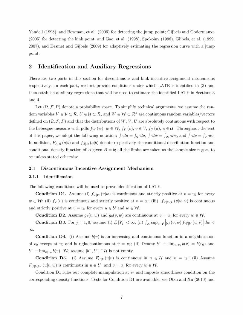
The following conditions will be used to prove identi�cation of LATE.

Condition D1. Assume (i) fV jW (vjw) is continuous and strictly positive at v = v0 for every

w 2 W; (ii) fV (v) is continuous and strictly positive at v = v0; (iii) fV jW;U (vjw; u) is continuousand strictly positive at v = v0 for every u 2 U and w 2 W.

Condition D2. Assume g1(v; w) and g0(v; w) are continuous at v = v0 for every w 2 W.Condition D3. For j = 1; 0, assume (i) E jYj j <1; (ii)

RW supv2V

���gj (v; w) fW jV (wjv)��� dw <

1.Condition D4. (i) Assume b(v) is an increasing and continuous function in a neighborhood

of v0 except at v0 and is right continuous at v = v0; (ii) Denote b+ � limv#v0 b(v) = b(v0) and

b� � limv"v0 b(v). We assume [b�; b+] \ U is not empty.

Condition D5. (i) Assume FU jV (ujv) is continuous in u 2 U and v = v0; (ii) Assume

FU jV;W (ujv; w) is continuous in u 2 U and v = v0 for every w 2 W.Condition D1 rules out complete manipulation at v0 and imposes smoothness condition on the

corresponding density functions. Tests for Condition D1 are available, see Otsu and Xu (2010) and

7

the references therein. Condition D2 imposes continuity at v0 of the potential outcome functions.

Condition D3 is a regularity condition. Let D (v) = I fb (v)� U � 0g for v 2 V. Then D = D (V )

and the propensity score is given by

P (v) � Pr (D = 1jV = v) = FU jV (b (v) jv) :

Condition D4 imposes conditions on the incentive assignment mechanism b. Without loss of gener-

ality, we assume in Condition D4 (i) that b(v) is increasing and right continuous at v = v0. Further

we assume in Condition D4 (ii) that [b�; b+] and the support of U are not mutually exclusive;

otherwise, the propensity score P (v) would be continuous at v = v0 taking values 0 or 1. Obviously

the incentive assignment mechanism b (v) = I fv � v0g satis�es Condition D4 as long as [0; 1]\U isnot empty. Condition D5 imposes smoothness conditions on the conditional distribution functions

of U . Under Conditions D4 and D5 (i), the propensity score is discontinuous at v0:

limv#v0

P (v) = FU jV (limv#v0

b (v) jv0) = FU jV (b+jv0) = FU jV (b(v0)jv0);

limv"v0

P (v) = FU jV (b�jv0):

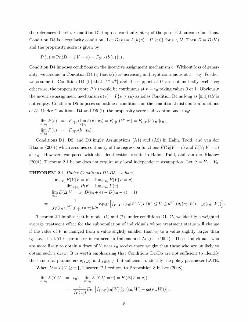
Conditions D1, D2, and D3 imply Assumptions (A1) and (A2) in Hahn, Todd, and van der

Klaauw (2001) which assumes continuity of the regression functions E(Y0jV = v) and E(Y1jV = v)

at v0. However, compared with the identi�cation results in Hahn, Todd, and van der Klaauw

(2001), Theorem 2.1 below does not require any local independence assumption. Let � = Y1 � Y0.

THEOREM 2.1 Under Conditions D1-D5, we have

limv#v0 E(Y jV = v)� limv"v0 E(Y jV = v)

limv#v0 P (v)� limv"v0 P (v)

= lime#0

E(�jV = v0; D(v0 + e)�D(v0 � e) = 1)

=1

fV (v0)R b+b� fU jV (ujv0)du

EW;UhfV jW;U (v0jW;U)I

�b� � U � b+

(g1(v0;W )� g0(v0;W ))

i:

Theorem 2.1 implies that in model (1) and (2), under conditions D1-D5, we identify a weighted

average treatment e�ect for the subpopulation of individuals whose treatment status will change

if the value of V is changed from a value slightly smaller than v0 to a value slightly larger than

v0, i.e., the LATE parameter introduced in Imbens and Angrist (1994). Those individuals who

are more likely to obtain a draw of V near v0 receive more weight than those who are unlikely to

obtain such a draw. It is worth emphasizing that Conditions D1-D5 are not su�cient to identify

the structural parameters g1, g0, and fW;U jV , but su�cient to identify the policy parameter LATE.

When D = I fV � v0g, Theorem 2.1 reduces to Proposition 3 in Lee (2008):

limv#v0

E(Y jV = v0)� limv"v0

E(Y jV = v) = E (�jV = v0)

=1

fV (v0)EW

hfV jW (v0jW ) (g1(v0;W )� g0(v0;W ))

i:

8

In this case, we identify a weighted average treatment e�ect for the entire population and this

weighted average treatment e�ect is identical to � = E (�jV = v0).

Proof of Theorem 2.1. Take v+ 2 V and v� 2 V such that v+ > v0 > v�. We will look at

E(Y jV = v+) and E(Y jV = v�) separately. Under condition D4 (i), b(v+) � b(v�).

First, we have

E(Y jV = v+)

= E(Y jV = v+; D(v+) = 1; D(v�) = 0)Pr(D(v+) = 1; D(v�) = 0jV = v+)

+E(Y jV = v+; D(v+) = 1; D(v�) = 1)Pr(D(v+) = 1; D(v�) = 1jV = v+)

+E(Y jV = v+; D(v+) = 0; D(v�) = 0)Pr(D(v+) = 0; D(v�) = 0jV = v+)

+E(Y jV = v+; D(v+) = 0; D(v�) = 1)Pr(D(v+) = 0; D(v�) = 1jV = v+)

= E(Y1jV = v+; D(v+) = 1; D(v�) = 0)Pr(D(v+) = 1; D(v�) = 0jV = v+)

+E(Y1jV = v+; D(v+) = 1; D(v�) = 1)Pr(D(v+) = 1; D(v�) = 1jV = v+)

+E(Y0jV = v+; D(v+) = 0; D(v�) = 0)Pr(D(v+) = 0; D(v�) = 0jV = v+)

+E(Y0jV = v+; D(v+) = 0; D(v�) = 1)Pr(D(v+) = 0; D(v�) = 1jV = v+):

Now from Condition D5 (i), we obtain:

limv+;v�!v0

Pr(Di(v+) = 1; Di(v�) = 0jVi = v+)

= limv+;v�!v0

Pr (b (v�) < Ui � b (v+) jVi = v+)

= Pr�b� < Ui � b+jVi = v0

�:

Similarly, we obtain:

limv+;v�!v0

Pr(D(v+) = 1; D(v�) = 1jV = v+) = Pr�U � b�jV = v0

�;

limv+;v�!v0

Pr(D(v+) = 0; D(v�) = 0jV = v+) = Pr�U > b+jV = v0

�;

limv+;v�!v0

Pr(D(v+) = 0; D(v�) = 1jV = v+) = Pr�b+ < U � b�jV = v0

�= 0:

As a result,

limv+!v0

E(Y jV = v+)

=

�lim

v+;v�!v0E(Y1jV = v+; b (v�) < U � b (v+))

�Pr�b� < U � b+jV = v0

�+

�lim

v+;v�!v0E(Y1jV = v+; U � b (v�))

�Pr�U � b�jV = v0

�+

�lim

v+;v�!v0E(Y0jV = v+; U > b

�v+�)

�Pr�U > b+jV = v0

�:

9

Similarly, we can show:

limv�!v0

E(Y jV = v�)

=

�lim

v+;v�!v0E(Y0jV = v�; b (v�) < U � b (v+))

�Pr�b� < U � b+jV = v0

�+

�lim

v+;v�!v0E(Y1jV = v�; U � b (v�))

�Pr�U � b�jV = v0

�+

�lim

v+;v�!v0E(Y0jV = v�; U > b

�v+�)

�Pr�U > b+jV = v0

�:

Lemma A.2 implies that for j = 1; 0:

limv+;v�!v0

E(Yj jV = v+; b (v�) < U � b (v+)) = limv+;v�!v0

E(Yj jV = v�; b (v�) < U � b (v+))

= E(Yj jV = v0; b� < U � b+);

limv+;v�!v0

E(Yj jV = v+; U � b (v�)) = limv+;v�!v0

E(Yj jV = v�; U � b (v�))

= E(Yj jV = v0; U � b�);

and

limv+;v�!v0

E(Yj jV = v+; U > b (v+)) = limv+;v�!v0

E(Yj jV = v�; U > b (v+))

= E(Yj jV = v0; U > b+):

Thus,

limv+!v0 E(Y jV = v+)� limv�!v0 E(Y jV = v�)

limv#v0 P (v)� limv"v0 P (v)

= E(Y1jV = v0; b� < U � b+)� E(Y0jV = v0; b

� < U � b+)

= limv+;v�!v0

E(�jV = v0; D(v+)�D(v�) = 1):

Finally let A = fb� < Ui � b+g. It follows from Lemma A.1 that for j = 1; 0,

E(Yj jV = v0; b� < U � b+)

=

Zgj(v0; w)fW jV;U (wjv0; A)dw

=

Zgj(v0; w)

R b+b� fV jW;U (v0jw; u)fW;U (w; u)dufV (v0)

R b+b� fU jV (ujv0) du

dw

= EW;U

24 fV jW;U (vjW;U)fV (v0)

R b+b� fU jV (ujv0) du

I�b� � U � b+

gj(v0;W )

35 :Q.E.D.

10

2.1.2 Auxiliary Regressions

In this subsection, we present conditions on the structural parameters in (1) and (2) to justify the

auxiliary regressions below:

Y = g(V ) + �IfV � v0g+ "; (4)

D = h(V ) + �IfV � v0g+ �; (5)

where E ("jV ) = 0, E (�jV ) = 0, and

� = limv#v0

E(Y jV = v)� limv"v0

E(Y jV = v); � = limv#v0

P (v)� limv"v0

P (v):

Unlike Porter (2003) and Imbens and Kalyanaramang (2009) who directly assume continuity of g

and h, we impose su�cient conditions on the structural parameters in (1) and (2) to ensure that g

and h are continuous on the support of V .

Condition D1(A). Assume (i) fV jW (vjw) is continuous and strictly positive on V for everyw 2 W; (ii) fV (v) is continuous and strictly positive on V; (iii) fV jW;U (vjw; u) is continuous andstrictly positive on V for u 2 U and w 2 W.

Condition D2(A). Assume g1(v; w) and g0(v; w) are continuous on V for every w 2 W.Condition D4(A). b(v) is continuous in v 2 V except at v0.Condition D5(A). (i) Assume FU jV (ujv) is continuous in u 2 U and v 2 V; (ii) Assume

FU jV;W (ujv; w) is continuous in u 2 U and v 2 V for every w 2 W.

Proposition 2.2 Under Conditions D1(A), D2(A), D3, D4, D4(A), and D5(A), the functions g(�)and h(�) are continuous on the support of V .

Remark 2.1. It is clear from the proof of Proposition 2.2 that under Conditions D1-D5, the

functions g(�) and h(�) are continuous at v0. For the jump wavelet estimator introduced in Section3, it is su�cient that g(�) and h(�) are continuous at v0.

2.2 Kink Incentive Assignment Mechanism

2.2.1 Identi�cation

Many policy assignment mechanisms including allocation of unemployment bene�ts and income

tax systems violate Condition D4. Instead they satisfy Condition K4 below.

Condition K1. Assume (i) fV jW (vjw) is continuously di�erentiable in a neighborhood of v0and fV jW (v0jw) > 0 for every w 2 W; (ii) fV (v) is continuously di�erentiable in a neighborhood ofv0 and fV (v0) > 0; (iii) fV jW;U (vjw; u) is continuously di�erentiable in a neighborhood of v0 andfV jW;U (v0jw; u) > 0 for u 2 U and w 2 W.

Condition K2. Assume g1(v; w) and g0(v; w) are continuously di�erentiable in a neighborhood

of v0 for every w 2 W.

11

Condition K3. For j = 1; 0, assume (i) E jYj j <1;(ii) For all u 2 U , supv j

@fUjV (ujv)@v j <1 and

Rsupv j

@fUjV (ujv)@v jdu <1;

(iii) For all w 2 W,Rsupv j

@fW;UjV (w;ujv)@v jdu <1 and

R Rsupv j

@fW;UjV (w;ujv)@v jdudw <1.

Condition K4. (i) Assume b(v) is increasing and continuously di�erentiable in a neighborhood

of v0 except at v0, where its derivative is right continuous at v = v0; (ii) b(v0) 2 U .Condition K5. (i) Assume FU jV (ujv) is continuously di�erentiable in u 2 U , and continu-

ously di�erentiable in a neighborhood of v0 as well; (ii) Assume FU jV;W (ujv; w) is continuouslydi�erentiable in u 2 U and continuously di�erentiable in a neighborhood of v0 for every w 2 W.

We note that Condition K4 is also used in Card, Lee, and Pei (2009) which assumes D = b (V )

implying a continuous treatment D under Condition K4. Instead we focus on a binary treatment

D and allow for the unobserved covariate U to a�ect the agent's selection of treatment status.

Denote b0+ � limv#v0 b0(v) = b0(v0) <1 and b0� � limv"v0 b

0(v) <1. Condition K4 (i) implies:b0� 6= b0+. Under Conditions K4 and K5 (i), the propensity score is discontinuous in its �rst

derivative at v0. To see this, we note that

P 0 (v) = fU jV (b(v)jv)b0(v) +@FU jV (b (v) jv)

@v:

So under conditions K4 and K5, we obtain:

limv#v0

P 0(v) = fU jV (b(v0)jv0)b0+ +Z b(v0)

�1

@fU jV (ujv0)@v

du;

limv"v0

P 0(v) = fU jV (b(v0)jv0)b0� +Z b(v0)

�1

@fU jV (ujv0)@v

du;

and

limv#v0

P 0(v)� limv"v0

P 0(v) = fU jV (b(v0)jv0)�b0+ � b0�

�6= 0:

THEOREM 2.3 Under Conditions K1-K5, we have

limv#v0 dE(Y jV = v)=dv � limv"v0 dE(Y jV = v)=dv

limv#v0 P0(v)� limv"v0 P

0(v)

= lime#0

E(�jV = v0; D(v0 + e)�D(v0 � e) = 1)

= EW

"[g1(v0;W )� g0(v0;W )]

fW jU;V (W jb(v0); v0)fW (W )

#:

2.2.2 Auxiliary Regressions

For kink incentive assignment mechanisms, we establish the following auxiliary regressions:

Y = gK(V ) + �K(V � v0)IfV � v0g+ "K ; (6)

D = hK(V ) + �K(V � v0)IfV � v0g+ �K : (7)

12

where E("K jV ) = 0, E(�K jV ) = 0, and

�K = limv#v0

dE(Y jV = v)=dv � limv"v0

dE(Y jV = v)=dv;

�K = limv#v0

P 0(v)� limv"v0

P 0(v):

Condition K1(A). Assume (i) fV jW (vjw) is continuously di�erentiable on V for every w 2 W;(ii) fV (v) is continuously di�erentiable on V; (iii) fV jW;U (vjw; u) is continuously di�erentiable onV for u 2 U and w 2 W.

Condition K2(A). Assume g1(v; w) and g0(v; w) are continuously di�erentiable on V for everyw 2 W.

Condition K4(A). b(v) is continuously di�erentiable for v 2 V except at v0, where it is onlycontinuous.

Condition K5(A). (i) Assume FU jV (ujv) is continuously di�erentiable in both u 2 U and

v 2 V; (ii) Assume FU jV;W (ujv; w) is continuously di�erentiable in both u 2 U and v 2 V for

every w 2 W.

Proposition 2.4 Under Conditions K1(A), K2(A), K3, K4, K4(A), and K5(A), the functions

gK(�) and hK(�) are continuously di�erentiable on V.

3 The First Wavelet Estimator

Let � denote the identi�ed LATE parameter. In this and the next sections, we propose wavelet

estimators of LATE for both discontinuous and kink incentive assignment mechanisms. Throughout

this and the next sections, we assume the conditions of Propositions 2.2 and 2.4 hold respectively

for discontinuous and kink incentive assignment mechanisms and a random sample (Vi; Yi; Di),

i = 1; :::; n, is available.

3.1 Discontinuous Incentive Assignment Mechanism

Under discontinuous incentive assignment mechanism, LATE is identi�ed as � = �=�, where � and

� are respectively the parameters in the auxiliary regressions (4) and (5). Since the idea underlying

the estimation of � and � is the same, we focus on the estimation of �.

The wavelet estimator of � we propose in this section is closely related to the estimator of the

jump size of the regression function E (YijVi = v) studied in Park and Kim (2006). Let FV (�) denotethe distribution function of Vi and � � FV (v0). Let V1:n � � � � � Vn:n denote the order statistics

of fVigni=1 andnY[i:n]

oni=1

the concomitants of fVi:ngni=1 or induced order statistics. Further letti = i=n for 1 � i � n.

13

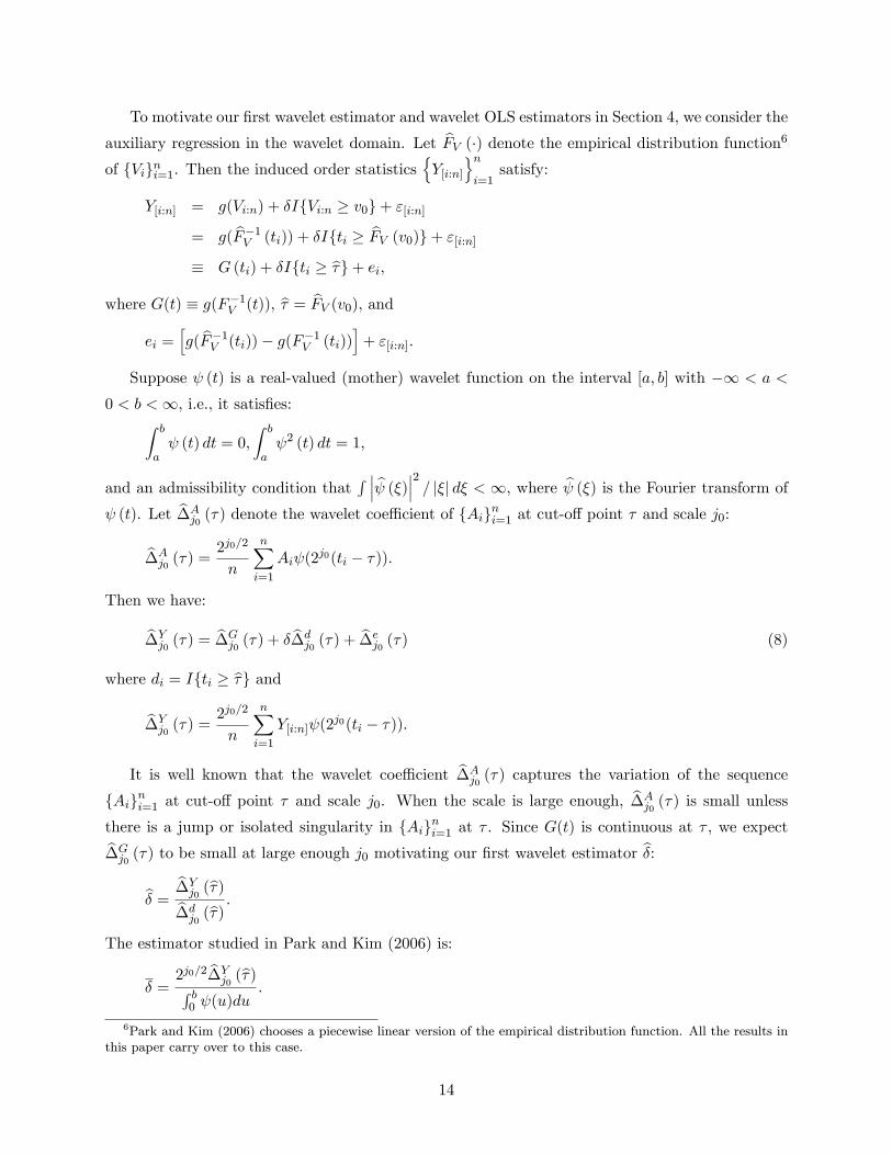
To motivate our �rst wavelet estimator and wavelet OLS estimators in Section 4, we consider the

auxiliary regression in the wavelet domain. Let bFV (�) denote the empirical distribution function6of fVigni=1. Then the induced order statistics

nY[i:n]

oni=1

satisfy:

Y[i:n] = g(Vi:n) + �IfVi:n � v0g+ "[i:n]= g( bF�1V (ti)) + �Ifti � bFV (v0)g+ "[i:n]� G (ti) + �Ifti � b�g+ ei;

where G(t) � g(F�1V (t)), b� = bFV (v0), andei =

hg( bF�1V (ti))� g(F�1V (ti))

i+ "[i:n]:

Suppose (t) is a real-valued (mother) wavelet function on the interval [a; b] with �1 < a <

0 < b <1, i.e., it satis�es:Z b

a (t) dt = 0;

Z b

a 2 (t) dt = 1;

and an admissibility condition thatR ��� b (�)���2 = j�j d� < 1, where b (�) is the Fourier transform of

(t). Let b�Aj0(�) denote the wavelet coe�cient of fAigni=1 at cut-o� point � and scale j0:

b�Aj0 (�) =

2j0=2

n

nXi=1

Ai (2j0(ti � �)):

Then we have:

b�Yj0 (�) =

b�Gj0 (�) + �

b�dj0 (�) +

b�ej0 (�) (8)

where di = Ifti � b�g andb�Yj0 (�) =

2j0=2

n

nXi=1

Y[i:n] (2j0(ti � �)):

It is well known that the wavelet coe�cient b�Aj0(�) captures the variation of the sequence

fAigni=1 at cut-o� point � and scale j0. When the scale is large enough, b�Aj0(�) is small unless

there is a jump or isolated singularity in fAigni=1 at � . Since G(t) is continuous at � , we expectb�Gj0(�) to be small at large enough j0 motivating our �rst wavelet estimator b�:b� = b�Y

j0(b�)b�d

j0(b�) :

The estimator studied in Park and Kim (2006) is:

� =2j0=2 b�Y

j0(b�)R b

0 (u)du:

6Park and Kim (2006) chooses a piecewise linear version of the empirical distribution function. All the results inthis paper carry over to this case.

14

To establish asymptotic properties of b�, we adopt the following assumptions. We note that the function needs to satisfy assumption A4 only. All wavelet functions satisfy A4, but functions

satisfying A4 may not be wavelet functions. For the ease of exposition, we will refer to any

function satisfying A4 as a `wavelet' function, the corresponding transform coe�cients as `wavelet'

coe�cients, and our estimators as wavelet estimators.

Assumption A1. A random sample (Vi; Yi; Di), i = 1; :::; n, is available.

Assumption A2.

(G). Let G(t) � g(F�1V (t)). (a) G(t) is lG times continuously di�erentiable for t 2 (0; 1)nf�g,and G(�) is continuous at � with �nite right and left-hand derivatives to order lG � m + 1; (b)

Right and left hand derivatives of G(t) up to order lG � m+ 1 are equal at � , where m is de�ned

in Assumption A4.

(H). Let H(t) � h(F�1V (t)). (a) H (t) is lH times continuously di�erentiable for t 2 (0; 1)nf�g,and H (�) is continuous at � with �nite right and left-hand derivatives to order lH � m + 1; (b)

Right and left hand derivatives of H (t) to order lH � m+ 1 are equal at � , where m is de�ned in

Assumption A4.

Assumption A3. (G). (a) �2"(v) � E("2jV = v) is continuous at v 6= v0 and its right and

left-hand limits at v0 exist; (b) For some � > 0, E[j"j2+� jv] is uniformly bounded on the support ofV .

(H). (a) �2� (v) � E(�2jV = v) is continuous at v 6= v0 and its right and left-hand limits at v0

exist; (b) For some � > 0, E[j�j2+� jv] is uniformly bounded on the support of V .(GH). �"� (v) � E("i�ijVi = v) is continuous at v 6= v0 and its right and left-hand limits at v0

exist.

Assumption A4. (a) The function (�) is continuous with compact support [a; b], wherea < 0 < b andm vanishing moments, i.e.,

R ba u

j (u) du = 0 for j = 0; 1; :::;m�1; (b)R b0 (u)du 6= 0,R b

a um (u) du 6= 0, and

R ba jum (u)j du <1; (c) has a bounded derivative.

Assumption A5. (a) As n!1, j0 !1, 2j0n ! 0, and 12j0

qn2j0! Ca <1; (b) As n!1,

j0 !1, 2j0n ! 0, and ( 12j0)mq

n2j0! Cb <1.

Assumption A1 may be relaxed to allow for non i.i.d. data by using the extension of Theorem

1 in Yang (1981) presented in Chu and Jacho-Chavez (2010). Assumption A2(G) (a) allows for

jumps in the derivatives of G at � up to order lG. Work in the statistics literature on detection of

jumps such as Wang (1995) and Park and Kim (2006) assume away the presence of jumps in the

derivatives of G at � so that Assumption A2(G) (b) holds. Assumption A3(G) imposes conditions

on the conditional variance function and E[j"j2+� jv]. Park and Kim (2006) assumes a constant

conditional variance function. Assumption A4 speci�es the class of functions . In contrast to a

kernel function which integrates to one, the function integrates to zero and shares the properties

of an m-th order kernel otherwise. Examples of include wavelet functions such as the class of

15

Daubechies' compactly supported wavelet functions D(L) and the class of least asymmetric wavelet

functions LA(L), where m = L and [a; b] = [� (L� 1) ; L]. In addition, the second derivativefunctions of kernel functions constructed in Cheng and Raimondo (2008) for which [a; b] = [�1; 1]and m = s � 1 and the di�erences between the two kernel functions used in Wu and Chu (1993)also satisfy Assumption A47. Assumption A5 imposes conditions on the scale j0.

THEOREM 3.1 Suppose A1, A3(G), and A4 hold.

(i) When A2(G) (a) and A5 (a) hold, we obtain:q

n2j0(b� � �) and

qn2j0(� � �) have the same

asymptotic distribution andrn

2j0(b� � �) d! N (CaBa; V ) ;

where

Ba =

hG(1)+ (�)�G

(1)� (�)

i R b0 (u)uduR b

0 (u)du;

V =�2"+(v0)

R b0

2(u)du+ �2"�(v0)R 0a

2(u)du�R b0 (u)du

�2 :

(ii) When A2(G) (b) and A5 (b) hold, we obtain:q

n2j0(b� � �) and

qn2j0(� � �) have the same

asymptotic distribution andrn

2j0(b� � �) d! N (CbBb; V ) ;

where

Bb =G(m)(�)

R ba u

m (u)duR b0 (u)du

:

When �2" (v) is a constant, the asymptotic distribution of � given in Theorem 3.1 (ii) reduces

to that in Park and Kim (2006). Theorem 3.1 (i) reveals a similar asymptotic behavior of b� tothe Nadaraya-Watson kernel estimator in Porter (2003) under A2(G) (a). However, as revealed in

Theorem 3.1 (ii), although A2(G) (b) does not a�ect the asymptotic distribution of the Nadaraya-

Watson kernel estimator in Porter (2003), it does a�ect the asymptotic distribution of our wavelet

estimator b�. In particular, it reduces the order of the asymptotic bias of b� from 2�j0 to 2�mj0 .

Thus, in terms of asymptotic bias, b� behaves more like the partial linear estimator of Porter (2003).This is not surprising, given that we transformed our covariates fVigni=1 to equally spaced designftigni=1 and the observation in Eubank and Speckman (1994) that for equally spaced design, theirpartial linear estimator of the jump size is asymptotically equivalent to an estimator similar to �

with a speci�c function. In general, transforming a random design to an equally spaced �xed

7See Assumption C1;s in Cheng and Raimondo (2008).

16

design before applying nonparametric method leads to better �nite sample performance, see Hall,

et al. (1998). In our context, this also leads to estimators that are design-adaptive: the asymptotic

bias and variance of our estimators do not depend on the density fV (v). In addition, the discrete

version of our estimator can be computed by applying the Cascades Algorithm by Mallat (2009).

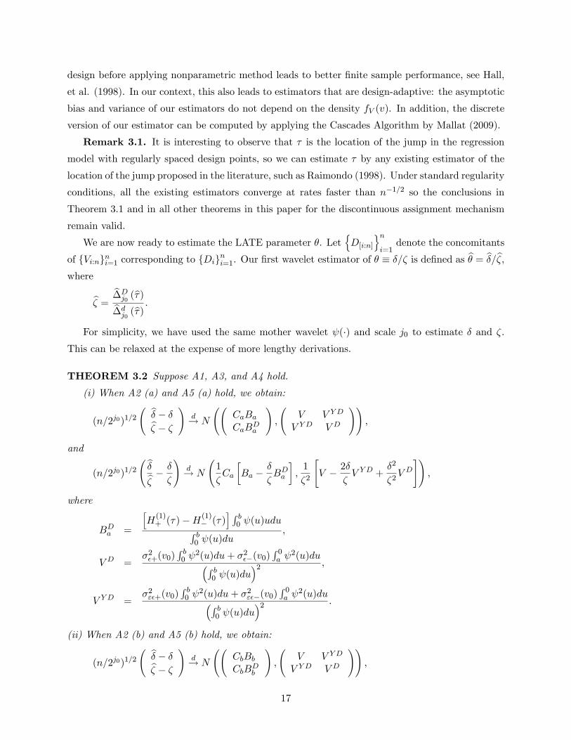
Remark 3.1. It is interesting to observe that � is the location of the jump in the regression

model with regularly spaced design points, so we can estimate � by any existing estimator of the

location of the jump proposed in the literature, such as Raimondo (1998). Under standard regularity

conditions, all the existing estimators converge at rates faster than n�1=2 so the conclusions in

Theorem 3.1 and in all other theorems in this paper for the discontinuous assignment mechanism

remain valid.

We are now ready to estimate the LATE parameter �. LetnD[i:n]

oni=1

denote the concomitants

of fVi:ngni=1 corresponding to fDigni=1. Our �rst wavelet estimator of � � �=� is de�ned as b� = b�=b�,where

b� = b�Dj0(b�)b�d

j0(b�) :

For simplicity, we have used the same mother wavelet (�) and scale j0 to estimate � and �.This can be relaxed at the expense of more lengthy derivations.

THEOREM 3.2 Suppose A1, A3, and A4 hold.

(i) When A2 (a) and A5 (a) hold, we obtain:

(n=2j0)1=2 b� � �b� � �

!d! N

CaBaCaB

Da

!;

V V Y D

V Y D V D

!!;

and

(n=2j0)1=2 b�b� � �

�

!d! N

1

�Ca

�Ba �

�

�BDa

�;1

�2

"V � 2�

�V Y D +

�2

�2V D

#!;

where

BDa =

hH(1)+ (�)�H(1)

� (�)i R b0 (u)uduR b

0 (u)du;

V D =�2�+(v0)

R b0

2(u)du+ �2��(v0)R 0a

2(u)du�R b0 (u)du

�2 ;

V Y D =�2"�+(v0)

R b0

2(u)du+ �2"��(v0)R 0a

2(u)du�R b0 (u)du

�2 :

(ii) When A2 (b) and A5 (b) hold, we obtain:

(n=2j0)1=2 b� � �b� � �

!d! N

CbBbCbB

Db

!;

V V Y D

V Y D V D

!!;

17

and

(n=2j0)1=2 b�b� � �

�

!d! N

1

�Cb

�Bb �

�

�BDb

�;1

�2

"V � 2�

�V Y D +

�2

�2V D

#!;

where

BDb =

H(m)(�)R ba u

m (u)duR b0 (u)du

:

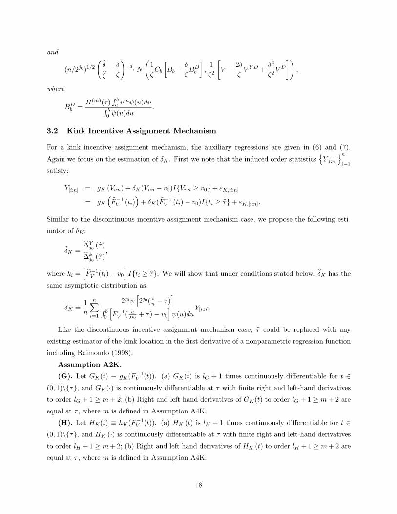
3.2 Kink Incentive Assignment Mechanism

For a kink incentive assignment mechanism, the auxiliary regressions are given in (6) and (7).

Again we focus on the estimation of �K . First we note that the induced order statisticsnY[i:n]

oni=1

satisfy:

Y[i:n] = gK (Vi:n) + �K(Vi:n � v0)IfVi:n � v0g+ "K;[i:n]= gK

� bF�1V (ti)�+ �K( bF�1V (ti)� v0)Ifti � b�g+ "K;[i:n]:

Similar to the discontinuous incentive assignment mechanism case, we propose the following esti-

mator of �K :

b�K = b�Yj0(b�)b�k

j0(b�) ;

where ki =h bF�1V (ti)� v0

iIfti � b�g. We will show that under conditions stated below, b�K has the

same asymptotic distribution as

�K =1

n

nXi=1

2j0 h2j0( in � �)

iR b0

hF�1V ( u

2j0+ �)� v0

i (u)du

Y[i:n]:

Like the discontinuous incentive assignment mechanism case, b� could be replaced with anyexisting estimator of the kink location in the �rst derivative of a nonparametric regression function

including Raimondo (1998).

Assumption A2K.

(G). Let GK(t) � gK(F�1V (t)). (a) GK(t) is lG + 1 times continuously di�erentiable for t 2

(0; 1)nf�g, and GK(�) is continuously di�erentiable at � with �nite right and left-hand derivativesto order lG + 1 � m+ 2; (b) Right and left hand derivatives of GK(t) to order lG + 1 � m+ 2 are

equal at � , where m is de�ned in Assumption A4K.

(H). Let HK(t) � hK(F�1V (t)). (a) HK (t) is lH + 1 times continuously di�erentiable for t 2

(0; 1)nf�g, and HK (�) is continuously di�erentiable at � with �nite right and left-hand derivativesto order lH + 1 � m+ 2; (b) Right and left hand derivatives of HK (t) to order lH + 1 � m+ 2 are

equal at � , where m is de�ned in Assumption A4K.

18

Assumption A4K. (a) The function (�) is continuous with compact support [a; b], wherea < 0 < b and m+1 vanishing moments, i.e.,

R ba u

j (u) du = 0 for j = 0; 1; :::;m; (b)R b0 u (u)du 6=

0,R ba u

m+1 (u) du 6= 0, andR ba

��um+1 (u)�� du <1; (c) has a bounded derivative.Assumption A5K. (a) As n ! 1, j0 ! 1, 23j0n ! 0, and 1

2j0

qn23j0

! CKa < 1; (b) As

n!1, j0 !1, 23j0n ! 0, and ( 12j0)mq

n23j0

! CKb <1.Assumption A6K. (a) F�1V (v) is continuously di�erentiable on the support of V ; (b) F�1V (v)

is m times continuously di�erentiable on the support of V .

THEOREM 3.3 Suppose A1, A3(G) for "K , and A4K hold.

(i) When A2K(G) (a), A5K (a) and A6K (a) hold, we obtain:q

n23j0

(b�K��K) and q n23j0

(�K��K) have the same asymptotic distribution andr

n

23j0(b�K � �K) d! N (CKaBKa; VK) ;

where

BKa =

hG(2)K+(�)�G

(2)K�(�)

i R b0 u

2 (u)du

2R b0 u (u)du

fV (v0);

VK =f2V (v0)

h�2"+(v0)

R b0

2(u)du+ �2"�(v0)R 0a

2(u)dui

�R b0 u (u)du

�2 :

(ii) When A2K(G) (b), A5K (b) and A6K (b) hold, we obtain:q

n23j0

(b�K��K) and q n23j0

(�K��K)have the same asymptotic distribution andr

n

23j0(b�K � �K) d! N (CKbBKb; VK) ;

where

BKb =G(m+1)K (�)

R ba u

m+1 (u)du

(m+ 1)!R b0 u (u)du

fV (v0):

Comparing Theorems 3.1 and 3.3, we observe the same qualitative behavior of b� and b�K in

terms of the order of their asymptotic bias: the order of the asymptotic bias of b�K depends on

whether there are jump discontinuities in the second and higher order derivatives of GK .

Finally our �rst LATE estimator for kink incentive assignment mechanisms is de�ned as b�K=b�K ,where b�K = b�D

j0(b�) = b�k

j0(b�).

THEOREM 3.4 Suppose A1, A3 for "K and �K , and A4K hold.

(i) When A2K (a), A5K (a) and A6K(a) hold, we obtain:rn

23j0

b�Kb�K � �K�K

!d! N

1

�CKa

�BKa �

�

�BDKa

�;1

�2

"VK �

2�

�V Y DK +

�2

�2V DK

#!;

19

where

BDKa =

hH(2)K+(�)�H

(2)K�(�)

i R b0 u

2 (u)du

2R b0 u (u)du

fV (v0);

V DK =

f2V (v0)h�2�+(v0)

R b0

2(u)du+ �2��(v0)R 0a

2(u)dui

�R b0 u (u)du

�2 ;

V Y DK =

f2V (v0)h�2"�+(v0)

R b0

2(u)du+ �2"��(v0)R 0a

2(u)dui

�R b0 u (u)du

�2 :

(ii) When A2K (b), A5K (b) and A6K(b) hold, we obtain:rn

23j0

b�Kb�K � �K�K

!d! N

1

�CKb

�BKb �

�

�BDKb

�;1

�2

"VK �

2�

�V Y DK +

�2

�2V DK

#!;

where

BDKb =

H(m+1)K (�)

R ba u

m+1 (u)du

(m+ 1)!R b0 u (u)du

fV (v0):

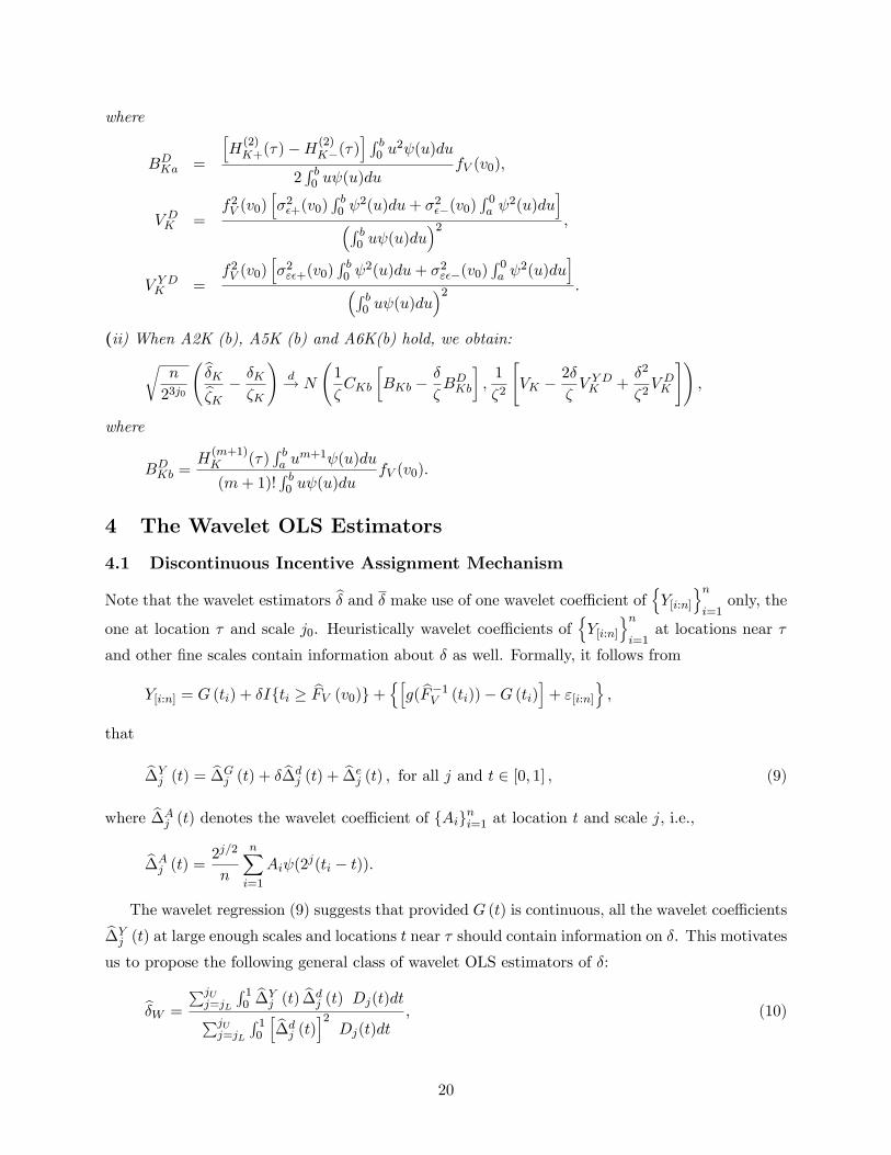
4 The Wavelet OLS Estimators

4.1 Discontinuous Incentive Assignment Mechanism

Note that the wavelet estimators b� and � make use of one wavelet coe�cient of nY[i:n]oni=1

only, the

one at location � and scale j0. Heuristically wavelet coe�cients ofnY[i:n]

oni=1

at locations near �

and other �ne scales contain information about � as well. Formally, it follows from

Y[i:n] = G (ti) + �Ifti � bFV (v0)g+ nhg( bF�1V (ti))�G (ti)i+ "[i:n]

o;

that

b�Yj (t) =

b�Gj (t) + �

b�dj (t) +

b�ej (t) ; for all j and t 2 [0; 1] ; (9)

where b�Aj (t) denotes the wavelet coe�cient of fAig

ni=1 at location t and scale j, i.e.,

b�Aj (t) =

2j=2

n

nXi=1

Ai (2j(ti � t)):

The wavelet regression (9) suggests that provided G (t) is continuous, all the wavelet coe�cientsb�Yj (t) at large enough scales and locations t near � should contain information on �. This motivates

us to propose the following general class of wavelet OLS estimators of �:

b�W =

PjUj=jL

R 10b�Yj (t)

b�dj (t) Dj(t)dtPjU

j=jL

R 10

h b�dj (t)

i2Dj(t)dt

; (10)

20

where Dj(t) � Ifa � 2j(b� � t) � bg is the `cone of in uence', see p. 215 in Mallet (2009), jL � jU ,

and jL � jLn !1 as n!1.The class of estimators in (10) include estimators using wavelet coe�cients at a single scale and

multiple locations, at multiscale and a single location, and at multiscale and multiple locations.

We'll establish the asymptotic properties of these estimators in the rest of this section and then

extend them to the corresponding results for estimators of LATE.

4.1.1 One scale with many locations

In this part, we consider the asymptotic properties of a subclass of wavelet OLS estimators for

which only one scale is used. The �xed scale j0 wavelet OLS estimator of � is de�ned as:

b�W1 =

R 10b�Yj0(t) b�d

j0(t)Dj0(t)dtR 1

0

h b�dj0(t)i2Dj0(t)dt

:

Assumption A5. (b)' As n!1, j0 !1, 2j0n ! 0, and�12j0

�2m�1qn2j0! CbW1 <1.

THEOREM 4.1 Suppose A1, A3(G), and A4 hold. In addition,R 0a�bM(v)dv 6= 0, where M (�)

is de�ned below.

(i) When A2(G) (a) and A5 (a) hold, we obtain:rn

2j0(b�W1 � �) d! N (CaB

aW1; VW1) ;

where

BaW1 =

hG(1)+ (�)�G

(1)� (�)

i R ba

R ba L(t) (s)(s� t)Ifs� t � 0gdsdtR 0a�bM(v)dv

;

VW1 =�2+(v0)

R b�a0 M2(v)dv + �2�(v0)

R 0a�bM

2(v)dvhR 0a�bM(v)dv

i2 ;

in which

L(t) =

Z b

aIfw � tg (w)dw and M(v) =

Z b

a

Z b

aIfw � t+ vg (w) (t)dtdw:

(ii) When A2(G) (b) with lG � 2m and A5 (b)' hold, we obtainrn

2j0(b�W1 � �) d! N

�CbW1B

bW1; VW1

�;

where

BbW1 =

G(2m�1)(�)R ba (s)s

mdsR ba L(t)(�t)m�1dt

m!(m� 1)!R 0a�bM(v)dv

:

21

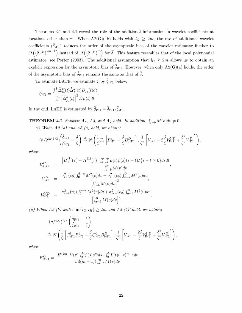
Theorems 3.1 and 4.1 reveal the role of the additional information in wavelet coe�cients at

locations other than � . When A2(G)( b) holds with lG � 2m, the use of additional wavelet

coe�cients (b�W1) reduces the order of the asymptotic bias of the wavelet estimator further to

O��2�j0

�2m�1�instead of O

��2�j0

�m�for b�. This feature resembles that of the local polynomial

estimator, see Porter (2003). The additional assumption that lG � 2m allows us to obtain an

explicit expression for the asymptotic bias of b�W1. However, when only A2(G)(a) holds, the order

of the asymptotic bias of b�W1 remains the same as that of b�.To estimate LATE, we estimate � by b�W1 below:

b�W1 =

R 10b�Dj0(t) b�d

j0(t)Dj0(t)dtR 1

0

h b�dj0(t)i2Dj0(t)dt

:

In the end, LATE is estimated by b�W1 = b�W1=b�W1.

THEOREM 4.2 Suppose A1, A3, and A4 hold. In addition,R 0a�bM(v)dv 6= 0.

(i) When A2 (a) and A5 (a) hold, we obtain:

(n=2j0)1=2 b�W1b�W1

� �

�

!d! N

1

�Ca

�BaW1 �

�

�BDaW1

�;1

�2

"VW1 � 2

�

�V Y DW1 +

�2

�2V DW1

#!;

where

BDaW1 =

hH(1)+ (�)�H(1)

� (�)i R b

a

R ba L(t) (s)(s� t)Ifs� t � 0gdsdtR 0a�bM(v)dv

;

V DW1 =

�2�+(v0)R b�a0 M2(v)dv + �2��(v0)

R 0a�bM

2(v)dvhR 0a�bM(v)dv

i2 ;

V Y DW1 =

�2"�+(v0)R b�a0 M2(v)dv + �2"��(v0)

R 0a�bM

2(v)dvhR 0a�bM(v)dv

i2 :

(ii) When A2 (b) with min flG; lHg � 2m and A5 (b)' hold, we obtain:

(n=2j0)1=2 b�W1b�W1

� �

�

!d! N

1

�

�CbW1B

bW1 �

�

�CbW1B

DbW1

�;1

�2

"VW1 �

2�

�V Y DW1 +

�2

�2V DW1

#!;

where

BDbW1 =

H(2m�1)(�)R ba (s)s

mds �R ba L(t)(�t)m�1dt

m!(m� 1)!R 0a�bM(v)dv

:

22

4.1.2 Multiscale with a single location

We now investigate the role of using more than one scale in estimating the LATE parameter.8 First

we consider the estimator of �:

b�W2 =

PjUj=jL

b�Yj (b�) b�d

j (b�)PjUj=jL

h b�dj (b�)i2 ;

where jL < jU . Let (jU � jL) = Kn.

THEOREM 4.3 Suppose A1, A3(G), and A4 hold. In addition, suppose �2"+(v0) = �2"�(v0).9

(i) When A2(G) (a) and A5 (a) hold for jL and jU , we obtain:

if limn!1Kn <1, thenrn

2jL(b�W2 � �) d! N

0@CaBaW2;

V

2h1� (12)limKn+1

i1A ;

where

BaW2 =

�1 + (

1

2)limKn+1

�2Ba3;

if limn!1Kn =1, thenrn

2jL(b�W2 � �) d! N

�2

3CaBa;

V

2

�;

(ii) When A2(G) (b) and A5 (b) hold for jL and jU , we obtain:

if limn!1Kn <1, thenrn

2jL(b�W2 � �) d! N

0@CbBbW2;

V

2h1� (12)limKn+1

i1A ;

where

BbW2 =

h1� (12)

(m+1)(limKn+1)i

2h1� (12)limKn+1

i h1� (12)m+1

iBb;if limn!1Kn =1, thenr

n

2jL(b�W2 � �) d! N

0@Cb 1

2h1� (12)m+1

iBb; V2

1A :8This has the avor of Kotlyarova and Zinde-Walsh (2006, 2008) which average kernel density estimators using

di�erent bandwidths.9For notational compactness, we only report results when �2"+(v0) = �2"�(v0) in the main text. General results

without this assumption can be found in the proof of this theorem in Appendix C.

23

Theorems 3.1, 4.1, and 4.3 reveal the interesting e�ects of using additional information in wavelet

coe�cients at multiple scales and multiple locations. First, the multiple locations estimator b�W1

reduces the order of the asymptotic bias of b� under A2(G)( b); Second, the multiple scales estimatorb�W2 reduces the asymptotic bias and variance of the wavelet estimator b� only proportionally, butunder both A2(G)(a) and A2(G)(b).

To estimate the LATE parameter, we let

b�W2 =

PjUj=jL

b�Dj (�)

b�dj (�)PjU

j=jL

h b�dj (�)

i2 :

THEOREM 4.4 Suppose A1, A3, and A4 hold. In addition, suppose �2"+(v0) = �2"�(v0),

�2�+(v0) = �2��(v0), and �2"�+(v0) = �2"��(v0).

(a) When A2 (a) and A5 (a) hold for jL and jU , we obtain:

if limn!1Kn <1, then

(n=2jL)1=2 b�W2b�W2

� �

�

!

d! N

0@1�Ca

�BaW2 �

�

�BDaW2

�;V � 2�

� VY D + �2

�2V D

2h1� (12)limKn+1

i�2

1A ;where

BDaW2 =

�1 + (

1

2)limKn+1

�2BD

a

3;

if limn!1Kn =1, then

(n=2jL)1=2 b�W2b�W2

� �

�

!d! N

0@ 2

3�Ca

�Ba �

�

�BDa

�;V � 2�

� VY D + �2

�2V D

2�2

1A :(b) When A2 (b) and A5 (b) hold for jL and jU , we obtain:

if limn!1Kn <1, then

(n=2jL)1=2 b�W2b�W2

� �

�

!

d! N

0@1�Cb

�BbW2 �

�

�BDbW2

�;V � 2�

� VY D + �2

�2V D

2h1� (12)limKn+1

i�2

1A ;where

BDbW2 =

h1� (12)

(m+1)(limKn+1)i

2h1� (12)limKn+1

i h1� (12)m+1

iBDb ;

24

if limn!1Kn =1, then

(n=2jL)1=2 b�W2b�W2

� �

�

!

d! N

0@Cb 1

2�h1� (12)m+1

i �Bb � �

�BDb

�;V � 2�

� VY D + �2

�2V D

2�2

1A :4.1.3 Multiscale with many locations

We now establish the asymptotic distribution of the general estimator b�W in (10):

b�W =

PjUj=jL

R 10b�Yj (t)

b�dj (t)Dj(t)dtPjU

j=jL

R 10

h b�dj (t)

i2Dj(t)dt

:

Again for notational compactness, we only establish the asymptotic distribution of b�W under the

condition that �2"+(v0) = �2"�(v0).

THEOREM 4.5 Suppose A1, A3, and A4 hold. In addition, suppose �2"+(v0) = �2"�(v0).

(i) When A2(G) (a) and A5(a) hold for jL and jU , we obtain:

if limn!1Kn <1, thenrn

2jL(b�W � �) d! N (CaB

aW ; VW ) ;

where

BaW =

6

7

h1� (18)

limKn+1i

h1� (14)limKn+1

iBaW1;

VW =9

14

1� (18)limKn+1h

1� (14)limKn+1i2 VW1;

if limn!1Kn =1, thenrn

2jL(b�W � �) d! N (CaB

a�W ; V

�W ) ;

where

Ba�W =

6

7BaW1; V

�W =

9

14VW1:

(ii) When A2(G) (b) with lG � 2m and (A5) (b)' hold for jL and jU , we obtain:

if limn!1Kn <1, thenrn

2jL(b�W � �) d! N

�CbW1B

bW ; VW

�;

where

BbW =

3

4h1� (12)2m+1

i 1� (12)(2m+1)(limKn+1)

1� (14)limKn+1

G(2m�1)(�)R ba (s)s

mdsR ba L(t)(�t)m�1dt

m!(m� 1)!R 0a�bM(v)dv

;

25

if limn!1Kn =1, thenrn

2jL(b�W � �) d! N

�CbW1B

b�W ; V

�W

�;

where

Bb�W =

3

4h1� (12)2m+1

iG(2m�1)(�) R ba (s)smds R ba L(t)(�t)m�1dtm!(m� 1)!

R 0a�bM(v)dv

:

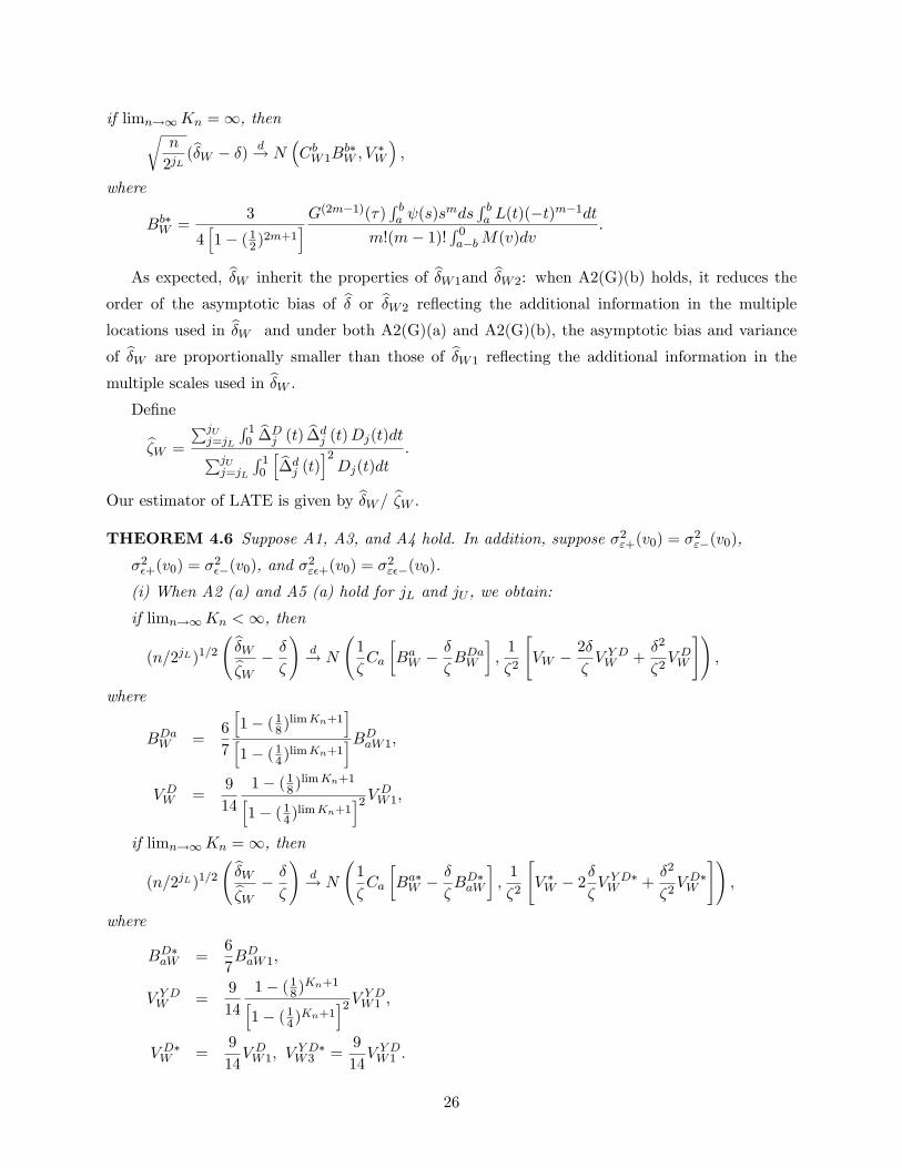
As expected, b�W inherit the properties of b�W1and b�W2: when A2(G)(b) holds, it reduces the

order of the asymptotic bias of b� or b�W2 re ecting the additional information in the multiple

locations used in b�W and under both A2(G)(a) and A2(G)(b), the asymptotic bias and variance

of b�W are proportionally smaller than those of b�W1 re ecting the additional information in the

multiple scales used in b�W .De�ne

b�W =

PjUj=jL

R 10b�Dj (t)

b�dj (t)Dj(t)dtPjU

j=jL

R 10

h b�dj (t)

i2Dj(t)dt

:

Our estimator of LATE is given by b�W = b�W .THEOREM 4.6 Suppose A1, A3, and A4 hold. In addition, suppose �2"+(v0) = �2"�(v0),

�2�+(v0) = �2��(v0), and �2"�+(v0) = �2"��(v0).

(i) When A2 (a) and A5 (a) hold for jL and jU , we obtain:

if limn!1Kn <1, then

(n=2jL)1=2 b�Wb�W � �

�

!d! N

1

�Ca

�BaW � �

�BDaW

�;1

�2

"VW � 2�

�V Y DW +

�2

�2V DW

#!;

where

BDaW =

6

7

h1� (18)

limKn+1i

h1� (14)limKn+1

iBDaW1;

V DW =

9

14

1� (18)limKn+1h

1� (14)limKn+1i2V D

W1;

if limn!1Kn =1, then

(n=2jL)1=2 b�Wb�W � �

�

!d! N

1

�Ca

�Ba�W � �

�BD�aW

�;1

�2

"V �W � 2�

�V Y D�W +

�2

�2V D�W

#!;

where

BD�aW =

6

7BDaW1;

V Y DW =

9

14

1� (18)Kn+1h

1� (14)Kn+1i2V Y D

W1 ;

V D�W =

9

14V DW1; V

Y D�W3 =

9

14V Y DW1 :

26

(ii) When A2 (b) with minflG; lHg � 2m and (A5)(b)' hold for jL and jU , we obtain:

if limn!1Kn <1, then

(n=2jL)1=2 b�Wb�W � �

�

!d! N

1

�Ca

�BbW � �

�BDbW

�;1

�2

"VW � 2�

�V Y DW +

�2

�2V DW

#!;

where

BDbW =

3

4h1� (12)2m+1

i 1� (12)(2m+1)(limKn+1)

1� (14)limKn+1

H(2m�1)(�)R ba (s)s

mdsR ba L(t)(�t)m�1dt

m!(m� 1)!R 0a�bM(v)dv

;

if limn!1Kn =1, then

(n=2jL)1=2 b�Wb�W � �

�

!d! N

1

�CbW1

�Bb�W � �

�BD�bW

�;1

�2

"V �W � 2�

�V Y D�W +

�2

�2V D�W

#!;

where

BD�bW =

3

4h1� (12)2m+1

iH(2m�1)(�)R ba (s)s

mdsR ba L(t)(�t)m�1dt

m!(m� 1)!R 0a�bM(v)dv

:

4.2 Kink Incentive Assignment Mechanism

All three wavelet OLS estimators for discontinuous incentive assignment mechanisms proposed in

Section 4.1 can be extended to kink incentive assignment mechanisms and they share the same

qualitative properties. To illustrate, we present a detailed analysis of the wavelet OLS estimator

based on wavelet coe�cients at a single scale and many locations and report results on the other

estimators in a separate paper.

Let

b�KW1 =

R 10b�Yj0(t) b�k

j0(t)Dj0(t)dtR 1

0

h b�kj0(t)i2Dj0(t)dt

and

�KW1 =1

n

nXi=1

JKW1(i

n)Yi:n

where

JKW1(i

n)

=

R 10

R 10 Dj0(t)

�F�1V (w)� v0

�Ifw � �g2j0

�2j0(w � t)

� h2j0( in � t)

idtdw

R 10

R 10

R 10

(Dj0(t)

�F�1V (w)� v0

�Ifw � �g

�F�1V (v)� v0

��Ifv � �g2j0

�2j0(w � t)

� �2j0(v � t)

� )dwdvdt

:

We �rst show that b�KW1 has the same asymptotic distribution as �KW1 and then establish the

asymptotic distribution of �KW1.

Assumption A5K. (b)' As n!1, j0 !1, 23j0n ! 0, and�12j0

�2m�1qn23j0

! CbK0W1 <1.Assumption A6K. (c) F�1V (v) is 2m times continuously di�erentiable on the support of V .

27

THEOREM 4.7 Suppose A1, A3(G), and A4K hold. Let M12 (s) = M1(s) +M2(s) � sM(s),

where

M(s) =

Z b

a

Z b

aIfw � t+ sg (w) (t)dtdw;

M1(s) =

Z b

a

Z b

a(�t)Ifw � t+ sg (w) (t)dtdw;

M2(s) =

Z b

a

Z b

awIfw � t+ sg (w) (t)dtdw:

AssumeR 0a�bM12 (t) dt 6= 0.

(i) When A2K(G) (a), A5K (a) and A6K(a) hold, we obtain:rn

23j0(b�KW1 � �K) d! N (CKaB

aKW1; VKW1) ;

where

BaKW1

= �

hG(2)K+(�)�G

(2)K�(�)

ifV (v0)

R ba

R ba (s� w)2 (s)Ifs� w � 0g [L1(w)� wL0(w)] dsdw

2R 0a�bM12 (t) dt

;

VKW1 =f2V (v0)

h�2"+(v0)

R 0a�bM

212 (t) dt+ �

2"�(v0)

R b�a0 M2

12 (t) dti

hR 0a�bM12 (t) dt

i2 ;

in which, for i = 0; 1; � � � ;m� 1, Li de�ned below has (m� i) vanishing moments:

Li(2j0(� � t)) =

Z b

awiIfw � 2j0(� � t)g (w)dw.

(ii) When A2K(G) (b) with lG � 2m, A5K (b)' and A6K(c) hold, we obtain:rn

23j0(b�kW1 � �k)

d! N�CbK0W1B

bKW1; VKW1

�;

where

BbKW1 = �f2V (v0)

R ba (s)s

m+1ds [�0 +Pmi=1 �i]R 0

a�bM12 (t) dt;

in which

�0 =

Z b

aL0(t)(�t)mdt

"mXi=1

[F�1V (�)](i)G(2m+1�i)K (�)

i!(m+ 1)!(m� i)!

#;

�i =1

i!

Z b

aLi(t)(�t)m�idt

"mXl=i

[F�1V (�)](l)G(2m�l+1)K (�)

(m� i)!(m+ 1)!(m� l)!

#for i � 1:

Now we provide the LATE estimator: b�KW1=b�KW1, where

b�KW1 =

R 10b�Dj0(t) b�k

j0(t)Dj0(t)dtR 1

0

h b�kj0(t)i2Dj0(t)dt

:

28

THEOREM 4.8 Suppose A1, A3, and A4K hold.

(a) When A2K (a), A5K (a) and A6K(a) hold, we obtain:rn

23j0

b�KW1b�KW1

� �K�K

!d! N

1

�CKa

�BaKW1 �

�

�BDaKW1

�;1

�2

"VKW1 �

2�

�V Y DKW1 +

�2

�2V DKW1

#!;

where

BDaKW1 = �

hH(2)K+(�)�H

(2)K�(�)

ifV (v0)

R ba

R ba (s� w)2 (s)Ifs� w � 0g [L1(w)� wL0(w)] dsdw

2R 0a�bM12 (t) dt

;

V DKW1 =

f2V (v0)h�2�+(v0)

R 0a�bM

212 (t) dt+ �

2��(v0)

R b�a0 M2

12 (t) dti

hR 0a�bM12 (t) dt

i2 ;

V Y DKW1 =

f2V (v0)h�2�"+(v0)

R 0a�bM

212 (t) dt+ �

2�"�(v0)

R b�a0 M2

12 (t) dti

hR 0a�bM12 (t) dt

i2 :

(b) When A2K (b) with min flG; lHg � 2m, A5K(b)' and A6K(c) hold, we obtain:rn

23j0

b�KW1b�KW1

� �K�K

!d! N

1

�CbK0W1

�BbKW1 �

�

�BDbKW1

�;1

�2

"VKW1 �

2�

�V Y DKW1 +

�2

�2V DKW1

#!;

where

BDbKW1 = �f2V (v0)

R ba (s)s

m+1ds [�0 +Pmi=1 �i]R 0

a�bM12 (t) dt,

in which

�0 =

Z b

aL0(t)(�t)mdt

"mXi=1

[F�1V (�)](i)H(2m+1�i)K (�)

i!(m+ 1)!(m� i)!

#;

�i =1

i!

Z b

aLi(t)(�t)m�idt

"mXl=i

[F�1V (�)](l)H(2m�l+1)K (�)

(m� i)!(m+ 1)!(m� l)!

#for i � 1.

5 Monte-Carlo Simulation

This section presents results from a small simulation study. We focus on the �nite sample perfor-

mances of our wavelet estimators of the jump size in two classes of models. The �rst class includes

switching regime models and the second class reduced form auxiliary regression models.

The two switching regime models are:

29

Model 1.

Y1 = 1:25 + V + V 2 +W1; Y0 = V + 2V 2 +W2;

D = IfV � 0:5g:

Model 2.

Y1 = 1 + V 7 +W1; Y0 = V 7 +W2;

D = IfV � 0:5g:

In both models, V � U [0; 1], (W1;W2) � N

"(0; 0);

0:01 00 0:01

!#, and V is independent of

(W1;W2). Lengthy algebras show that the corresponding auxiliary regression models are:

Model 1 : Y =

(V + 2V 2 +W , 0 � V < 0:5

1:25 + V + V 2 +W , 0:5 � V � 1 ;

and

Model 2 : Y =

(V 7 +W , 0 � V < 0:5

1 + V 7 +W , 0:5 � V � 1 ;

where W � N(0; 0:01). The auxiliary regression functions indicate that Model 1 satis�es A2(G)(a)

and Model 2 satis�es A2(G)(b).

We also generate data directly from the two auxiliary regression models below:

Model 3.

Y =

(V +W , 0 � V < 0:5

0:5 + 2V +W , 0:5 � V � 1 :

Model 4.

Y =

(V +W , 0 � V < 0:5

1 + V +W , 0:5 � V � 1 :

In both models, V � U [0; 1], W � N(0; 0:01), and V is independent of W . Obviously Model 3

satis�es A2(G)(a) and Model 4 satis�es A2(G)(b).

From each model, we generate random samples of sizes 500, 2; 500, 5; 000 respectively and

computed our wavelet estimates using Daub4. Daub4 has 4 vanishing moments supported on

[�3; 4]. All four estimators depend on the choice of the scale. For single scale estimators, we chosesix scale levels, 1; 2; 3; 4; 5; 6, while for many scales estimators, we chose jL = 1; 2; 3; 4; 5; 6 and

Kn = 2. We repeated this for 5; 000 times and computed the bias, standard deviation, and MSE

of each estimator. To save space, results for samples of sizes 500 and 2; 500 are reported in Tables

1-4.

Insert tables here.

30

Tables 1-4 reveal the same qualitative behavior of each estimator for all models. First, as the

sample size increases, the MSEs of all estimators decrease; Second, overall many locations estimatorb�W1 performs much better than the single location estimator b� in terms of bias, standard error, andMSE; Third, many scales estimator b�W2 performs better than the single scale estimator b�, but thereduction in MSE is not as much as that of the many locations estimator b�W1 in comparison with

the single scale and single location estimator b�; Fourth, for all estimators and all models, as thescale level increases, the MSE decreases initially and then begins to increase. It seems that for most

cases considered, the optimal scale level is either 3 or 4.10 Overall, the numerical results con�rm

our theoretical �ndings that it is advantageous to use more locations and more scales in estimating

the jump size compared with single scale and single location estimator currently available in the

literature and that our many scales and many locations estimator b�W performs the best whether

A2(G)(a) or A2(G)(b) holds.

6 Conclusion

In this paper, we have studied the identi�cation of LATE in two classes of switching regime models.

Both allow for individuals to make decision based on not only incentives assigned to them but also

their unobserved characteristics. The �rst class of switching regime models accounts for discon-

tinuous incentive assignment mechanisms and the second accounts for kink incentive assignment

mechanisms. For each class of switching regime models, we established auxiliary regressions for

estimating LATE based on which we have presented a systematic treatment of wavelet estimation

of LATE. In addition to making use of the existing wavelet estimator of the jump size or kink size,

we have developed new wavelet OLS estimators improving upon the existing wavelet estimator by

employing more wavelet transform coe�cients. The asymptotic properties of all the estimators are

established and their �nite sample properties are investigated via a simulation study.

This paper has focused on incentive assignment mechanisms depending on one forcing variable

and having a single known cut-o�. In some empirical applications, the cut-o� point may be unknown

to the econometrician and there may be more than one forcing variables. For example, Hoekstra

(2009) applied RDD to studying the e�ect of attending the agship state university on earnings.

For the university and data set he used, the admission's cut-o� depends on both SAT score and high

school GPA. Hoekstra (2009) constructed an adjusted SAT score for a given GPA and estimated a

parametric model with the adjusted SAT score as the forcing variable. Since the university didn't

keep records of the exact admission rules used, the cut-o� point is unknown and estimated. It

would be interesting to extend the wavelet OLS estimators proposed in this paper to allow for

unknown cut-o� and/or more than one forcing variables.

10We have limited results on the selection of the optimal scale. For space considerations, we will report details onthis in a separate paper.

31

This paper also suppresses other covariates X (say) in the potential outcomes equations and

the selection equation. An extension of the model (1) and (2) accounting for the presence of other

covariates is:

Y1 = g1 (X;V;W ) , Y0 = g0 (X;V;W ) , (11)

D = Ifb(V ) + g3 (X)� U � 0g, (12)

where g3 is an unknown function of X. Under appropriate conditions, the auxiliary regressions

established earlier for estimating LATE in both discontinuous and kink incentive assignment mech-

anisms still hold and our wavelet estimators still apply. Alternatively, one may take into account

the observable covariates X in estimating LATE. This may be done by making use of the alternative

auxiliary regressions:

Y = g(X;V ) + � (X) IfV � v0g+ ";

D = h (X;V ) + � (X) IfV � v0g+ �;

where E["jX;V ] = 0 and E[�jX;V ] = 0. Fr�olich (2007) proposes a local linear estimator taking

into account the covariate X and compares it with the local linear estimator without using X. The

asymptotic analysis in Fr�olich (2007) seems to suggest that using the covariate X may not always

improve the performance of the LATE estimator. It would be interesting to extend our wavelet

estimators to take into account the covariate X. We'll leave this to future research.

32

Appendix A: Technical Proofs and Lemmas Used in Section 2

Lemma A.1 For any a; b satisfying: �1 � a < b � 1 and [a; b] � U , we have:

fW jV;A(wjv;A) =R ba fV jW;U (vjw; u)fW;U (w; u)du

fV (v)R ba fU jV (ujv) du

,

where A = f a < U � bg.

Proof. By de�nition, we have

fW jV;A(wjv;A)

=1

Pr(a < U � bjV = v)

@fPr(W � wjV = v; a < U � b) Pr(a < U � bjV = v)g@w

=1

Pr(a < U � bjV = v)

@fPr(W � w; a < U � bjV = v)g@w

=1

Pr(a < U � bjV = v)

@

@w

(Z w

�1

Z b

afW;U jV (w

0; ujv)dw0du)

=1

Pr(a < U � bjV = v)

Z b

afW;U jV (w; ujv)du:

Q.E.D.

Lemma A.2 Under the conditions of Theorem 2.1, we get: for j = 0; 1,

limv+;v�!v0

E(Yj jV = v+; A (v+; v�)) = E(Yj jV = v0; A),

where fA (v+; v�) ; Ag = ffb (v�) < U � b (v+)g ; fb� < U � b+gg ; or ffU � b (v�)g ; fU � b�gg ;or ffU > b (v+)g ; fU > b+gg :

Proof. Without loss of generality, we provide the proof for j = 0 and

fA (v+; v�) ; Ag =�fb (v�) < U � b (v+)g ;

�b� < U � b+

:

By de�nition,

E(Y0jV = v+; A (v+; v�)) =Zg0(v+; w)fW jV;A(v+;v�)(wjv+; A (v+; v�))dw:

Lemma A.1 implies:

fW jV;A(v+;v�)(wjv+; A (v+; v�)) =R b(v+)b(v�)

fV jW;U (v+jw; u)fW;U (w; u)du

fV (v+)R b(v+)b(v�)

fU jV (ujv+) du:

Then

fW jV;A(v+;v�)(wjv+; A (v+; v�))

=

R b(v+)b(v�)

fU jV;W (ujv+; w)dufV;W (v+; w)

fV (v+)hFU jV (b (v+) jv+)� FU jV (b (v�) jv�)

i=

hFU jV;W (b (v+) jv+; w)� FU jV;W (b (v�) jv+; w)

ifV jW (v+jw) fW (w)

fV (v+)hFU jV (b (v+) jv+)� FU jV (b (v�) jv�)

i :

33

It follows from Conditions D1, D4 and D5 that

limv+;v�!v0

fW jV;A(v+;v�)(wjv+; A (v+; v�))

=limv+;v�!v0

nhFU jV;W (b (v+) jv+; w)� FU jV;W (b (v�) jv+; w)

ifV jW (v+jw) fW (w)

olimv+;v�!v0

nfV (v+)

hFU jV (b (v+) jv+)� FU jV (b (v�) jv�)

io=

[FU jV;W (b+jv0; w)� FU jV;W (b�jv0; w)] � fV jW (v0jw) � fW (w)h

FU jV (b+)� FU jV (b�)i� fV (v0)

=

R b+b� fV jW;U (v0jw; u)fW;U (w; u)dufV (v0)

R b+b� fU jV (ujv0) du

:

Thus by Condition D2, Condition D3, and the dominated convergence theorem, we get

limv+;v�!v0

E(Y0jV = v+; A (v+; v�))

= limv+;v�!v0

Zg0(v+; w)fW jV;A(v+;v�)(wjv+; A (v+; v�))dw

=

Zlim

v+;v�!v0g0(v+; w) lim

v+;v�!v0fW jV;A(v+;v�)(wjv+; A (v+; v�))dw

=

Zg0(v0; w)

R b+b� fV jW;U (v0jw; u)fW;U (w; u)dufV (v0)

R b+b� fU jV (ujv0) du

dw

= E(Y0jV = v0; A):

Q.E.D.

Proof of Proposition 2.2. The proofs for g and h are similar so we provide a proof for g only

and complete it in three steps:

Step 1. We prove continuity of g(�) at v0;Step 2. We prove continuity of g(v) at any v� < v0;

Step 3. We prove continuity of g(v) at any v� > v0.

Proof of Step 1. Note that

limv#v0

g(v) = limv#v0

E(Y jV = v)� � = limv"v0

E(Y jV = v) = limv"v0

g(v):

By de�nition, we have

g(v0)

= E(Y jV = v0)��limv#v0

E(Y jV = v)� limv"v0

E(Y jV = v)

�= E(Y jV = v0; b

� < U � b+) Pr(b� < U � b+jV = v0)

+E(Y jV = v0; U � b�) Pr(U � b�jV = v0)

+E(Y jV = v0; U > b+) Pr(U > b+jV = v0)

+E(Y jV = v0; b+ < U � b�) Pr(b+ < U � b�jV = v0)� (Y + � Y �)

= limv+!v0

E(Y jV = v+)��limv#v0

E(Y jV = v)� limv"v0

E(Y jV = v)

�= lim

v"v0E(Y jV = v):

34

Then g(v0) = limv#v0 g(v) = limv"v0 g(v):Proof of Step 2. For v� < v0, we know: g(v

�) = E(Y jV = v�). Then,

limv!v�

E(Y jV = v)

= limv!v�

[E(Y jV = v;D(v) = 1)Pr(D(v) = 1jV = v)]

+ limv!v�

[E(Y jV = v;D(v) = 0)Pr(D(v) = 0jV = v)]

= limv!v�

[E(Y1jV = v;D(v) = 1)Pr(D(v) = 1jV = v)]

+ limv!v�

[E(Y jV = v;D(v) = 0)Pr(D(v) = 0jV = v)]

= limv!v�

[E(Y1jV = v; U � b(v)) Pr(U � b(v)jV = v)]

+ limv!v�

[E(Y0jV = v; U > b(v)) Pr(U > b(v)jV = v)]

= limv!v�

[E(Y1jV = v; U � b(v))] Pr(U � limv!v�

b(v)jV = v�)

+ limv!v�

[E(Y0jV = v; U > b(v))] Pr(U > limv!v�

b(v)jV = v�)

= E(Y1jV = v�; U � limv!v�

b(v))] Pr(U � limv!v�

b(v)jV = v�)

+E(Y0jV = v�; U > limv!v�

b(v)) Pr(U > limv!v�

b(v)jV = v�)

= E(Y jV = v�);

where we have used:

limv!v�

[E(Y1jV = v; U � b(v))] = limv!v�

Zg1(v; w)fW jV;U�b(v)(wjv; U � b(v))dw

=

Zg1(v

�; w)

R limv!v� b(v)�1 fV jW;U (v

�jw; u)fW;U (w; u)dufV (v�)

R b(v�)�1 fU jV (ujv)du

dw;

= E(Y1jV = v�; U � limv!v�

b(v)]:

A similar argument leads to: limv!v� [E(Y0jV = v; U > b(v))] = E(Y0jV = v�; U > limv!v� b(v)).

Proof of Step 3. It is similar to that of Step 2 and thus omitted. Q.E.D.

Proof of Theorem 2.3. We complete the proof in two steps:

Step 1. We show:

lime#0

E(�jV = v0; D(v0 + e)�D(v0 � e) = 1)

= EW

"[g1(v0;W )� g0(v0;W )]

fW jU;V (W jb(v0); v0)fW (W )

#:

Step 2. We show:

limv#v0 dE(Y jV = v)=dv � limv"v0 dE(Y jV = v)=dv

limv#v0 P0(v)� limv"v0 P

0(v)

= EW

"[g1(v0;W )� g0(v0;W )]

fW jU;V (W jb(v0); v0)fW (W )

#:

Proof of Step 1. It follows from Condition K4(i):

lime#0

E(�jV = v0; D(v0 + e)�D(v0 � e) = 1)

= lime#0

E(�jV = v0; D(v0 + e) = 1; D(v0 � e) = 0):

35

The right hand side expression is:

= lime#0

E(g1(v0;W )� g0(v0;W )jV = v0; b(v0 + e) � U > b(v0 � e))

= lime#0

Z[g1(v0; w)� g0(v0; w)] fW jV;U (wjv0; b(v0 + e) � U > b(v0 � e))dw

= lime#0

Z[g1(v0; w)� g0(v0; w)]

24R b(v0+e)b(v0�e) fW;U jV (w; ujv0)duR b(v0+e)b(v0�e) fU jV (ujv0)du

35 dw=

Z[g1(v0; w)� g0(v0; w)] lim

e#0

24R b(v0+e)b(v0�e) fW;U jV (w; ujv0)duR b(v0+e)b(v0�e) fU jV (ujv0)du

35 dw=

Z[g1(v0; w)� g0(v0; w)]

fW;U jV (w; b(v0)jv0)fU jV (b(v0)jv0)

dw

=

Z[g1(v0; w)� g0(v0; w)] fW jU;V (wjb(v0); v0)dw

= EW

"[g1(v0;W )� g0(v0;W )]

fW jU;V (W jb(v0); v0)fW (W )

#;

where we have used the following result:

lime#0

24R b(v0+e)b(v0�e) fW;U jV (w; ujv0)duR b(v0+e)b(v0�e) fU jV (ujv0)du

35= lim

e#0

"e�1 fP (b(v0 + e))� P (b(v0))� (P (b(v0 � e))� P (b(v0)))ge�1 fQ(b(v0 + e))�Q(b(v0))� (Q(b(v0 � e))�Q(b(v0)))g

#

=fW;U jV (w; b(v0)jv0) [b0+(v)� b0�(v)]fU jV (b(v0)jv0) [b0+(v)� b0�(v)]

=fW;U jV (w; b(v0)jv0)fU jV (b(v0)jv0)

;

in which P (x)� P (a) =R xa fW;U jV (w; ujv0)du and Q(x)�Q(b) =

R xb fU jV (ujv0)du.

Proof of Step 2. Consider E(Y jV = v):

E(Y jV = v)

= E(Y1jV = v;D(v) = 1)Pr(D(v) = 1jV = v) + E(Y0jV = v;D(v) = 0)Pr(D(v) = 0jV = v)

=

" Rg1(v; w)fW jV;U (wjv; b(v) � u)dw

R b(v)�1 fU jV (ujv)du

+Rg0(v; w)fW jV;U (wjv; b(v) < u)dw

R1b(v) fU jV (ujv)du

#

=

Zg1(v; w)

R b(v)�1 fW;U jV (w; ujv)duR b(v)�1 fU jV (ujv)du

dw

Z b(v)

�1fU jV (ujv)du

+

Zg0(v; w)

R1b(v) fW;U jV (w; ujv)duR1

b(v) fU jV (ujv)dudw

Z 1

b(v)fU jV (ujv)du

=

Zg1(v; w)

Z b(v)

�1fW;U jV (w; ujv)dudw +

Zg0(v; w)

Z 1

b(v)fW;U jV (w; ujv)dudw:

36

Taking derivatives on both sides of the last equality above, we get:

dE(Y jV = v)

dv

=

Z@

@v

g1(v; w)

Z b(v)

�1fW;U jV (w; ujv)du

!dw +

Z@

@v

g0(v; w)

Z 1

b(v)fW;U jV (w; ujv)du

!dw

=

Zg01(v; w)

Z b(v)

�1fW;U jV (w; ujv)dudw +

Zg1(v; w)[b

0(v)fW;U jV (w; b(v)jv)

+

Zg00(v; w)

Z 1

b(v)fW;U jV (w; ujv)dudw +

Zg0(v; w)[�b0(v)fW;U jV (w; b(v)jv)

+

Z b(v)

�1

@

@v(fW;U jV (w; ujv))du]dw +

Z 1

b(v)

@

@v(fW;U jV (w; ujv))du]dw:

Now taking limits leads to

limv#v0

dE(Y jV = v)

dv

=

Zg01(v0; w)

Z b(v0)

�1fW;U jV (w; ujv0)dudw

+

Zg1(v0; w)[b

0+fW;U jV (w; b(v0)jv0) +Z b(v0)

�1

@

@v(fW;U jV (w; ujv0))du]dw

+

Zg00(v0; w)

Z 1

b(v0)fW;U jV (w; ujv0)dudw

+

Zg0(v0; w)[�b0+fW;U jV (w; b(v0)jv0) +

Z 1

b(v0)

@

@v(fW;U jV (w; ujv0))du]dw

and

limv"v0

dE(Y jV = v)

dv

=

Zg01(v0; w)

Z b(v0)

�1fW;U jV (w; ujv0)dudw

+

Zg1(v0; w)[b

0�fW;U jV (w; b(v0)jv0) +Z b(v0)

�1

@

@v(fW;U jV (w; ujv0))du]dw

+

Zg00(v0; w)

Z 1

b(v0)fW;U jV (w; ujv0)dudw

+

Zg0(v0; w)[�b0�fW;U jV (w; b(v0)jv0) +

Z 1

b(v0)

@

@v(fW;U jV (w; ujv0))du]dw:

As a result, we have:

limv#v0

dE(Y jV = v)

dv� limv"v0

dE(Y jV = v)

dv

=

Z[g1(v0; w)� g0(v0; w)] fW;U jV (w; b(v0)jv0)dw

�b0+ � b0�

�

37

and

limv#v0 dE(Y jV = v)=dv � limv"v0 dE(Y jV = v)=dv

limv#v0 P0(v)� limv"v0 P

0(v)

=

R[g1(v0; w)� g0(v0; w)] fW;U jV (w; b(v0)jv0)dw [b0+(v)� b0�(v)]

fU jV (b(v0)jv0) [b0+(v)� b0�(v)]

=

Z[g1(v0; w)� g0(v0; w)]

fW;U jV (w; b(v0)jv0)fU jV (b(v0)jv0)

dw:

Q.E.D.

Proof of Proposition 2.4. We provide a proof for gK only. This will be done in two steps:

Step 1. We show gK is continuous;

Step 2. We show gK is continuously di�erentiable.

Proof of Step 1. By de�nition, gK(V ) = E(Y jV ) � �K(V � v0)IfV � v0g. We only needto show that it is continuous at v0. Under Condition K4(A), we know: limv#v0 E(Y jV = v) �limv#v0 E(Y jV = v) = 0 = �; thus E(Y jV ) = g(v) from Proposition 2.2, which is continuous on the

support of V . Since �K(V �v0)IfV � v0g is continuous on the support of V , gK(V ) is continuous.Proof of Step 2. When v = v0,

limv#v0

dgK(v)

dv= lim

v#v0

dE(Y jV = v)

dv� �K = lim

v"v0

dE(Y jV = v)

dv

and limv"v0dgK(v)dv = limv"v0

dE(Y jV=v)dv : Thus

limv#v0

dgK(v)

dv= lim

v"v0

dgK(v)

dv= lim

v"v0

dE(Y jV = v)

dv= lim

v!v0

dg(v)

dv:

Now let us consider v� < v0. Then following the proof of Theorem 2.3 except that we are looking

at v� instead of v0, we obtain: limv#v� dE(Y jV = v)=dv � limv"v� dE(Y jV = v)=dv = 0: A similar

proof applies to v� > v0. Q.E.D.

38

Appendix B: Technical Proofs for Results in Section 3We will make extensive use of the following Taylor expansions in the proofs in Appendices B

and C. Under A2(G)(a), we have:

G(� � h) = G(�) +lG�1Xk=1

G(k)� (�)

k!(�h)k +R�G;

where G(k)� (�) denote the right and left k-th order derivatives of G(t) at � ,

jR�Gj � KjhjlG supt2(0;1)

jG(lG)� (t)j <1

with K a large positive number. Under A2(G)(b), we have:

G(� + h) = G(�) +lG�1Xk=1

G(k)(�)

k!(h)k +RG; (B.1)

where for a large positive number K, jRGj � KjhjlG supt2(0;1) jG(lG)(t)j <1:The proofs also rely heavily on Theorem 1 in Yang (1981). For completeness, we restate it in

Lemma B.1 below. Note that we need to extend Theorem 1 in Yang (1981) to allow the function J

below to depend on n as in Remark 2 in Yang (1981). Let (Xi; Yi) (i = 1; 2; :::; n) be independent

and identically distributed as (X;Y ). The rth ordered X variate is denoted by Xr:n and the Y

variate paired with it is denoted by Y[r:n]. Let

Sn = n�1nXi=1

J (i=n)Y[i:n];

where J is some bounded smooth function and may depend on n. Further, let

m(x) = E(Y jX = x); �2(x) = V ar(Y jX = x);

F�1(u) = inffxjF (x) � ug; m � F�1(u) = m(F�1(u)):

Lemma B.1 Suppose the following conditions are satis�ed: E(Y 2) <1; m(x) is a right continu-ous function of bounded variation in any �nite interval; J is bounded and continuous ae m � F�1;and the cdf of X, F (x), is a continuous function. Let

�2 =

Z +1

�1J2(F (x))�2(x)dF (x)

+

Z +1

�1

Z +1

�1[F (x ^ y)� F (x)F (y)]J(F (x))J(F (y))dm(x)dm(y):

Then limn!1 nV ar(Sn) = �2 and limn!1E(Sn) =R+1�1 m(x)J(F (x))dF (x). Furthermore, if

�2 > 0, then

Sn � E(Sn)pV ar(Sn)

d! N(0; 1):

We note that all the proposed wavelet estimators including the wavelet OLS estimators converge

at rates slower than n�1=2. Since b� converges at rate n�1=2, under regularity conditions, theasymptotic distributions of all our estimators are not a�ected by estimating � by b� . This is

universal to all nonparametric estimators constructed after a �rst step estimation of the location

39

of a jump or kink, see e.g., the work in statistics cited in Section 1 including Wang and Cai (2010).

Because of this, we will work with the infeasible versions of our estimators with b� replaced by � inAppendices B and C. With slight abuse of notation, we will use the same notations to denote the

corresponding infeasible estimators. For notational compactness, we let j [�] = 2j �2j ��in both

Appendix B and Appendix C.

Proof of Theorem 3.1. We will complete the proof in two steps:

Step 1. We show that � has the asymptotic distributions stated in the theorem;

Step 2. We show:q

n2j0(b� � �) = op (1).

Proof of Step 1: Note that we can write � as: � = 1n

Pni=1 J(

in)Y[i:n]; where

J(i

n) =

j0

hin � �

iR b0 (u)du

:

We will use Lemma B.1 to show thatq

n2j0(���) has the limiting distribution stated in Theorem 3.1.

The conditions in Lemma B.1 are satis�ed: E(Y jV = v) = g(v)+�Ifv � v0g is right continuous byProposition 2.2 and of bounded variation in any �nite interval; J( in) is bounded and continuous

by Assumption A4.

First, let us calculate limn!1E(�):Z +1

�1[g(v) + �Ifv � v0g]

j0(FV (v)� �)R b0 (u)du

dFV (v)

=

R+1�1 g(v) j0(FV (v)� �)dFV (v)R b

0 (u)du+

R+1�1 �Ifv � v0g j0(FV (v)� �)dFV (v)R b

0 (u)du

=

R ba ghF�1V ( u

2j0+ �)

i (u)duR b

0 (u)du+ �

=

( 1

2j0

hG(1)+ (�)�G(1)� (�)

i R b0 (u)uduR b

0 (u)du

+ � + s:o:, under A2(G)(a)

( 1

2j0)mG(m)(�)

R baum (u)duR b

0 (u)du

+ � + s:o, under A2(G)(b)

:

Then,

limn!1

2j0hE(�1)� �

i=

hG(1)+ (�)�G

(1)� (�)

i R b0 (u)uduR b

0 (u)du, under A2(G)(a),

limn!1

2mj0hE(�1)� �

i=

G(m)(�)R ba u

m (u)duR b0 (u)du

, under A2(G)(b).

Second, let us calculate limn!1 nV ar(�):Z +1

�1

" j0(FV (v)� �)R b

0 (u)du

#2�2(v)dFV (v)

+

Z +1

�1

Z +1

�1[FV (v1 ^ v2)� FV (v1)FV (v2)]

j0(FV (v1)� �) j0(FV (v2)� �)�R b0 (u)du

�2 dm(v1)dm(v2)

= A1 +A2;

40

where

m (v) = g(v) + �Ifv � v0g;

A1 =

Z +1

�1

" j0(FV (v)� �)R b

0 (u)du

#2�2(v)dFV (v);

A2 =

Z +1

�1

Z +1

�1[FV (v1 ^ v2)� FV (v1)FV (v2)]

j0(FV (v1)� �) j0(FV (v2)� �)�R b0 (u)du

�2 dm(v1)dm(v2):

Then

A1 =

Z +1

�1

"2j0 (u)R b0 (u)du

#2�2(F�1V (

u

2j0+ �))

1

2j0du

=2j0R+1�1 2(u)�2(F�1V ( u

2j0+ �))du�R b

0 (u)du�2

=2j0hR b0

2(u)�2(F�1V ( u2j0+ �))du+

R 0a

2(u)�2(F�1V ( u2j0+ �))du

i�R b0 (u)du

�2 :

So A1 = O(2j0) and A2 = O(1). Thus we get:

limn!1

n

2j0V ar(�) =

h�2+(v0)

R b0

2(u)du+ �2�(v0)R 0a

2(u)dui

�R b0 (u)du

�2 :

By Lemma B.1, we obtain:rn

2j0(�1 � �) d!

(N(CaBa; V ), under A2(G)(a)

N(CbBb; V ), under A2(G)(b):

Proof of Step 2: Note thatrn

2j0(b� � �)

=

rn

2j0�

R b0 (u)du� 1

n

Pnj=1 I ftj � �g j0 [tj � � ]

1n

Pnj=1 I ftj � �g j0 [tj � � ]

!;

where the �rst term satis�es:q

n2j0� = Op(

qn2j0): For large enough j0, the numerator of the second

term satis�es:

j 1n

nXj=1

I ftj � �g j0 [tj � � ]�Z b

0 (u)duj

= j 1n

nXj=1

I ftj � �g j0 [tj � � ]�Z 1

0I ft � �g j0 [tj � � ] dtj

� 1

n+ 1V 10 (f),

where the last inequality above is obtained from the Koksma{Hlawka inequality in which

f(t) = I ft � �g j0 [tj � � ]

41

and V 10 (f) is the bounded variation of f on [0; 1].

Note that for large enough j0,

V 10 (f) = V 1� ( j0 [� � � ]) = 2j0Z 1

�j2j0 (1)

h2j0(t� �)

ijdt

= 2j0Z b

0j (1) [t] jdt = O

�2j0�

sinceR b0 j (1) [t] jdt <1. Hence,rn

2j0(b� � �) =

rn

2j0�

R b0 (u)du

1n

Pnj=1 I ftj � �g j0 [tj � � ]

� 1!

= Op(

rn

2j0)Op(

2j0

n) = op(1).

Q.E.D.

Proof of Theorem 3.2. First, we derive the asymptotic covariance between b� and b�:limn!1

Covh(n=2j0)1=2(b� � �); (n=2j0)1=2(b� � �)i = lim

n!1n

2j0Cov

hb�; b�i= lim

n!1n

2j0Cov

"1

n

nXi=1

J(i

n)Y[i:n];

1

n

nXi=1

J(i

n)D[i:n]

#

=1

2j0

Z +1

�1J2(FV (x))�

2"�(x)dFV (x)

+1

2j0

Z +1

�1

Z +1

�1[FV (x ^ y)� FV (x)FV (y)]J(FV (x))J(FV (y))dm(x)dmD(y)

=

h�2"�+(v0)

R b0

2(u)du+ �2"��(v0)R 0a

2(u)dui

�R b0 (u)du

�2 ;

where mD(x) = E(DjV = x) and the second last equality follows from the proof of equation (8) in

Yang (1981).

Next, we apply the Cramer-Wold Device to establish the joint limiting distribution of

(n=2j0)1=2(b� � �) and (n=2j0)1=2(b� � �). In the end, we use Delta method to establish the

asymptotic distribution for b�=b�. Q.E.D.Proof of Theorem 3.3. First we work with the bias term for �K :Z +1

�1[gK(v) + �K(V � v0)Ifv � v0g]

j0(FV (v)� �)R b0

hF�1V ( u

2j0+ �)� v0

i (u)du

dFV (v)

=

R+1�1 gK(v) j0(FV (v)� �)dFV (v)R b0

hF�1V ( u

2j0+ �)� v0

i (u)du

+

R+1�1 �KvIfv � v0g j0(FV (v)� �)dFV (v)R b

0

hF�1V ( u

2j0+ �)� v0

i (u)du

=

R ba gK

hF�1V ( u

2j0+ �)

i (u)duR b

0

hF�1V ( u

2j0+ �)� v0

i (u)du

+ �K :

Under A2K(G)(a), we have

Z b

agK

�F�1V (

u

2j0+ �)

� (u)du =

hG(2)K+(�)�G

(2)K�(�)

i R b0 u

2 (u)du

22j0+1+ s:o:

42

Under A2K(G)(b):Z b

agK

�F�1V (

u

2j0+ �)

� (u)du =

G(m+1)K (�)

R ba u

m+1 (u)du

(m+ 1)!2(m+1)j0+ s:o:

and Z b

0

�F�1V (

u

2j0+ �)� v0

� (u)du =

R b0 u (u)du

2j0fV (v0)+ s:o:

Then,

limn!1

2j0hE(�K)� �K

i=

hG(2)K+(�)�G

(2)K�(�)

ifV (v0)

R b0 u

2 (u)du

2R b0 u (u)du

, under A2K(G)(a),

limn!1

2mj0hE(�K)� �K

i=

G(m+1)K (�)

(m+ 1)!

fV (v0)R ba u

m+1 (u)duR b0 u (u)du

, under A2K(G)(b).

Now we work on the variance term:

Z +1

�1

24 2j0 (u)R b0

hF�1V ( u

2j0+ �)� v0

i (u)du

352 �2(F�1V (u

2j0+ �))

1

2j0du

=2j0R+1�1 2(u)�2(F�1V ( u

2j0+ �))du�

12j0

1fV (v0)

R b0 u (u)udu

�2=

2j0�12j0

1fV (v0)

R b0 u (u)udu

�2"Z b

0 2(u)�2(F�1V (

u

2j0+ �))du+

Z 0

a 2(u)�2(F�1V (

u

2j0+ �))du

#:

Thus we get

limn!1

n

23j0V ar(�K) =

f2V (v0)h�2"+(v0)

R b0

2(u)du+ �2"�(v0)R 0a

2(u)dui

�R b0 u (u)du

�2 :

Finally the asymptotic normality of b�K is established by following a similar proof to that of

Theorem 3.1. Q.E.D.

43

Appendix C: Technical Proofs for Results in Section 4We recall j [�] = 2j

�2j ��and the following expressions for functions L (t) and M (v):

L(t) =

Z b

aIfw � tg (w)dw and M(v) =

Z b

a

Z b

aIfw � t+ vg (w) (t)dtdw:

Lemma C.1 Under Assumption (A4), (i) L(t) has (m� 1) vanishing moments and compact sup-port [a; b]; (ii) M(t) has compact support [a� b; b� a].

Proof of Lemma C.1. By induction. Q.E.D.

Proof of Theorem 4.1. Let

�W1 = n�1nXi=1

JW1

�i

n

�Y[i:n];

where

JW1(i

n) =

R 10

R 10 Dj0(t)Ifw � �g j0 [w � t] j0

hin � t

idtdwR 1

0

R 10

R 10 Dj0(t)Ifw � �gIfv � �g j0 [w � t] j0 [v � t] dwdvdt

:

We will complete the proof in two steps:

Step 1. We show �W1 has the asymptotic distributions stated in the theorem;

Step 2. We show:q

n2j0(b�W1 � �W1) = op (1).

Proof of Step 1: First, let us calculate limn!1E(�W1):Z 1

�1[g(v) + �Ifv � v0g]JW1(FV (v))dFV (v) =

Z 1

�1g(v)JW1(FV (v))dFV (v) + �:

For the �rst term on the right hand side of the above equation,Z 1

�1g(v)JW1(FV (v))dFV (v)

=2�j0

R1�1 g(v)

hR 10

R 10 Dj0(t)Ifw � �g j0 [w � t] j0 [FV (v)� t] dtdw

idFV (v)

2�j0R 10

R 10

R 10 Dj0(t)Ifw � �gIfv � �g j0 [w � t] j0 [v � t] dwdvdt

=TW1

TW1D;

where

TW1 = 2�j0Z 1

�1g(v)

�Z 1

0

Z 1

0Dj0(t)Ifw � �g j0 [w � t] j0 [FV (v)� t] dtdw

�dFV (v);

TW1D = 2�j0Z 1

0

Z 1

0

Z 1

0Dj0(t)Ifw � �gIfv � �g j0 [w � t] j0 [v � t] dwdvdt:

For large enough j0, we obtain:

TW1 =

Z 1

0

Z 1

0

"Z b

ag(F�1V (

s

2j0+ t)) (s)ds

#Dj0(t)Ifw � �g

h2j0(w � t)

idtdw

=

Z 1

0

Z 1

0W (t)Dj0(t)Ifw � �g

h2j0(w � t)

idtdw

=1

2j0

Z 1

0

"Z b

aIfw � 2j0(� � t)g [w] dw

#Dj0(t)W (t)dt

=1

2j0

Z 1

0L(2j0(� � t))Dj0(t)W (t)dt

= (1

2j0)2Z b

aL(t)W (� � t

2j0)dt;

44

where

W (t) �Z b

aG

�s

2j0+ t

� (s)ds:

Ignoring higher order terms, we obtain: under A2(G)(a):

W (� � t

2j0) =

Z b

aG

�� +

s� t2j0

� (s)ds

=

Z b

aG

�� +

s� t2j0

� (s)Ifs� t

2j0� 0gds+

Z b

aG

�� +

s� t2j0

� (s)Ifs� t

2j0< 0gds

=lG�1Xk=1

G(k)+ (�)

k!

Z b

a(s� t2j0

)k (s)Ifs� t2j0

� 0gds+lG�1Xk=1

G(k)� (�)

k!

Z b

a(s� t2j0

)k (s)Ifs� t2j0

< 0gds:

Then,

TW1 = (1

2j0)3hG(1)+ (�)�G

(1)� (�)

i Z b

a

Z b

aL(t) (s)(s� t)Ifs� t � 0gdsdt:

Under A2(G)(b):

W (� � t

2j0) =

lG�1Xk=1

G(k)(�)

k!

Z b

a(s� t2j0

)k (s)ds+ s:o:

Then,

TW1 = (1

2j0)2lG�1Xk=1

G(k)(�)

k!

Z b

a

Z b

aL(t) (s)(

s� t2j0

)kdsdt+ s:o:

=

(( 12j0)2m+1G

(2m�1)(�)m!(m�1)!

R ba (s)s

mdsR ba L(t)(�t)m�1dt+ s:o: if lg � 2m;

O(( 12j0)lG+2) if lg < 2m:

For large enough j0,

TW1D =

Z 1

0

Z 1

0

"Z b

aIfw � 2j0(� � t)g [w] dw

#Dj0(t)Ifv � �g

h2j0(v � t)

idtdv

=

Z 1

0

Z 1

0L(2j0(� � t))Ifa � 2j0(� � t) � bgIfv � �g

h2j0(v � t)

idtdv

=1

2j0

Z 1

0

"Z b

aL(2j0(� � v) + t) (t)dt

#Ifv � �gdv

=1

2j0

Z 1

0M(2j0(� � v))Ifv � �gdv

=1

22j0

Z 0

a�bM(v)dv:

Therefore, under A2(G)(a):

TW1

TW1D=( 12j0)hG(1)+ (�)�G

(1)� (�)

i R ba

R ba L(t) (s)(s� t)Ifs� t � 0gdsdtR 0

a�bM(v)dv+ s:o:;

45

under A2(G)(b):

TW1

TW1D=

8><>:( 1

2j0)2m�1�G(2m�1)(�)

R ba (s)smds�

R baL(t)(�t)m�1dt

m!(m�1)!R 0a�bM(v)dv

+ s:o: if lG � 2m

O(( 12j0)lG) if lG < 2m

:

Thus, under A2(G)(a), we obtain:

limn!1

2j0hE(�W1)� �

i=

hG(1)+ (�)�G

(1)� (�)

i R ba

R ba L(t) (s)(s� t)Ifs� t � 0gdsdtR 0a�bM(v)dv

;

under A2(G)(b), we obtain:

limn!1(2j0)2m�1hE(�W1)� �

i=

G(2m�1)(�)R ba (s)smds�

R baL(t)(�t)m�1dt

m!(m�1)!R 0a�bM(v)dv

, if lG � 2m;

limn!1(2j0)lGhE(�W1)� �

i= O(1), if lG < 2m:

Second, let us calculate the asymptotic variance of �W1:R1�1

hR 10

R 10 Dj0(t)Ifw � �g j0 [w � t]

�2j0(FV (v)� t)

�dtdw

i2�2(v)dFV (v)

T 2D

+

R R 8>><>>:[FV (v1 ^ v2)� FV (v1)FV (v2)]�

�hR 10

R 10 Dj0(t)Ifw � �g j0 [w � t]

�2j0(FV (v1)� t)

�dtdw

i�hR 10

R 10 Dj0(t)Ifw � �g j0 [w � t]

�2j0(FV (v2)� t)

�dtdw

i9>>=>>; dm(v1)dm(v2)

T 2D

=TW12

T 2W1D

+TW13

T 2W1D

;

where

TW12 =

Z 1

�1

�Z 1

0

Z 1

0Dj0(t)Ifw � �g j0 [w � t]

h2j0(FV (v)� t)

idtdw

�2�2(v)dFV (v);

TW13 =

Z +1

�1

Z +1

�1

8>><>>:[FV (v1 ^ v2)� FV (v1)FV (v2)]hR 1

0

R 10 Dj0(t)Ifw � �g j0 [w � t]

�2j0(FV (v1)� t)

�dtdw

ihR 10

R 10 Dj0(t)Ifw � �g j0 [w � t]

�2j0(FV (v2)� t)

�dtdw

i9>>=>>; dm(v1)dm(v2):

For the TW12 term

TW12 =

Z 1

0P 2W1 (u)�

2(F�1V (u))du;

where

PW1 (u) =

Z 1

0

Z 1

0Dj0(t)Ifw � �g j0 [w � t]

h2j0(u� t)

idtdw:

Notice that for large enough j0;

PW1 (u) =

Z 1

0

"Z b

aIfw � 2j0(� � t)g (w)dw

#Dj0(t)

h2j0(u� t)

idt

=

Z 1

0L(2j0(� � t))Dj0(t)

h2j0(u� t)

idt

=1

2j0M(2j0(� � u)):

46

Therefore,

TW12 =1

23j0

Z b�a

a�bM2(u)�2(F�1(� � u

2j0))du:

Notice that when n!1, TW12

T 2W1D= O(2j0), while TW13

T 2W1D= O(1).

In the end,

limn!1

n

2j0V ar(�W1) =

R b�aa�b M

2(u)�2(F�1(� � u2j0))duhR b�a

a�b M(v)Ifv � 0gdvi2

=�2+(v0)

R b�a0 M2(v)dv + �2�(v0)

R 0a�bM

2(v)dvhR 0a�bM(v)dv

i2 :

Proof of Step 2: Note thatrn

2j0(b�W1 � �W1) =

rn

2j0

�1

n

Pni=1 (Ai � Ci)Yi:n

B

�+

rn

2j0�W1

�D

B� 1

�;

where

Ai =

Z 1

0

1

n

nXj=1

Iftj � �g j0 [tj � t] h2j0(ti � t)

iDj0(t)dt;

B =

Z 1

0

24 1n

nXj=1

2j0=2Iftj � �g h2j0(tj � t)

i352Dj0(t)dt;

Ci =

Z 1

0

Z 1

0Dj0(t)Ifw � �g j0 [w � t]

h2j0(ti � t)

idtdw;

D =

Z 1

0

Z 1

0

Z 1

0Dj0(t)Ifw � �gIfv � �g j0 [w � t]

h2j0(v � t)

idwdvdt:

For the termq

n2j0�W1

hDB � 1

i, note that

limn!1

jB �Dj

� limn!1

Z 1

0

������ 1nnXj=1

2j0=2Iftj � �g h2j0(tj � t)

i�Z 1

02j0=2Ifw � �g

h2j0(w � t)

idw

�������

������ 1nnXj=1

2j0=2Iftj � �g h2j0(tj � t)

i+

Z 1

02j0=2Ifv � �g

h2j0(v � t)

idv

������Dj0(t)dt

� limn!1

supt2D(t)

2j0=2

������ 1nnXj=1

Iftj � �g h2j0(tj � t)

i�Z 1

0Ifw � �g

h2j0(w � t)

idw

������� supt2D(t)

2j0=2

������ 1nnXj=1

Iftj � �g h2j0(tj � t)

i+

Z 1

0Ifv � �g

h2j0(v � t)

idv

������Z 1

0Dj0(t)dt

= O(2j0=2

n) �O( 1

2j0=2) �O( 1

2j0)

= O(1

n2j0):

47

Thus,rn

2j0�W1

�D

B� 1

�= op(1):

Since D = O( 122j0

) from TW1D term, thus B = O( 122j0

). And note thatrn

2j0

"1

n

Pni=1 (Ai � Ci)Y[i:n]

B

#

�r

n

2j01

Bsupt2D(t)

����� 1n

Pnj=1 Iftj � �g j0 [tj � t]

�R 10 Ifw � �g j0 [w � t] dw

����� 1nnXi=1

Z 1

0Dj0(t)dt sup

t2D(t)

��� h2j0(ti � t)i���Y[i:n]=

rn

2j01

Bsupt2D(t)

����� 1n

Pnj=1 Iftj � �g j0 [tj � t]

�R 10 Ifw � �g j0 [w � t] dw

����� 1nnXi=1

supt2D(t)

j j0 [ti � t]jY[i:n]R 10 Dj0(t)dt

2j0

= O(

rn

2j0) �O(22j0) �O(2

j0

n) �Op(1) �O(

1

22j0)

= Op(

s2j0

n) = op(1):

In the end, we have:q

n2j0(b�W1 � �W1) = op (1) : Q.E.D.

Proof of Theorem 4.3: We begin with the simplest case where jL = j0 and jU = j0 + 1.

Then by induction we prove the general case.

When jL = j0, and jU = j0 + 1, we have:

b�W2 =b�Yj0(�) b�d

j0(�) + b�Y

j0+1(�) b�d

j0+1(�)h b�d

j0(�)i2+h b�d

j0+1(�)i2

=

1n

Pni=1

(1n

Pnl=1 Iftl � �g j0 [tl � � ] [2j0(ti � �)]

+ 2n

Pnl=1 Iftl � �g j0 [2(tl � �)] [2j0+1(ti � �)]

)Y[i:n]h

2j0=2

n

Pnl=1 Iftl � �g [2j0(ti � �)]

i2+h2(j0+1)=2

n

Pnl=1 Iftl � �g [2j0+1(ti � �)]

i2 :Let

�W2 =1

n

nXi=1

JW2(i

n)Y[i:n];

where

JW2(i

n) =

2j0n [2j0( in � �)] + [2

j0+1( in � �)]o

(1 + 12)R b0 (t)dt

:

We will complete the proof in two steps:

Step 1. We show �W2 has the asymptotic distributions stated in the theorem;

Step 2. We showq

n2j0(b�W2 � �W2) = op (1).

Proof of Step 1: FirstZ 1

�1[g(v) + �Ifv � v0g]JW2(FV (v))dFV (v) =

Z 1

�1g(v)JW2(FV (v))dFV (v) + �

=2

3

Z 1

�1g(v)

j0 [FV (v)� � ]R b0 (t)dt

dFV (v) +1

3

Z 1

�1g(v)

2 j0 [2(FV (v)� �)]R b0 (t)dt

dFV (v) + �

=2

3P1 +

1

3P2 + �;

48

where

P1 =

Z 1

�1g(v)

j0 [FV (v)� � ]R b0 (t)dt

dFV (v);

P2 =

Z 1

�1g(v)

2 j0 [2(FV (v)� �)]R b0 (t)dt

dFV (v):

From the proof of Theorem 3.1, we know: under A2(G)(a):

P1 =

12j0

hG(1)+ (�)�G

(1)� (�)

i R b0 (u)uduR b

0 (u)du+ s:o:;

P2 =

12j0+1

hG(1)+ (�)�G

(1)� (�)

i R b0 (u)uduR b

0 (u)du+ s:o:

Then,

2

3P1 +

1

3P2 =

52j0

hG(1)+ (�)�G

(1)� (�)

i R b0 (u)udu

6R b0 (u)du

+ s:o:

Again from the proof of Theorem 3.1, we know: under A2(G)(b):

P1 =( 12j0)mG(m)(�)

R ba u

m (u)duR b0 (u)du

+ s:o:;

P2 =( 12j0+1

)mG(m)(�)R ba u

m (u)duR b0 (u)du

+ s:o:

Then,

2

3P1 +

1

3P2 =

( 12j0)m(2 + 1

2m )G(m)(�)

R ba u

m (u)du

3R b0 (u)du

+ s:o:

Thus when Kn = 1,

limn!1

2j0hE(�W2)� �

i=

5hG(1)+ (�)�G

(1)� (�)

i R b0 (u)udu

6R b0 (u)du

, under A2(G)(a);

limn!1

2mj0hE(�W2)� �

i=

(2 + 12m )G

(m)(�)R ba u

m (u)du

3R b0 (u)du

, under A2(G)(b).

Second, let us calculate limn!1 nV ar(�W2) with Kn = 1:Z 1

�1

"2j0� [2j0(FV (v)� �)] + [2j0+1(FV (v)� �)]

(1 + 1

2)R b0 (t)dt

#2�2(v)dFV (v)

+

Z +1

�1

Z +1

�1

8>>>><>>>>:[FV (v1 ^ v2)� FV (v1)FV (v2)](

j0 [FV (v1)� � ]+ j0 [2(FV (v1)� �)]

)( j0 [FV (v2)� � ]

+ j0 [2(FV (v2)� �)]

)h32

R b0 (t)dt

i29>>>>=>>>>; dm(v1)dm(v2)

= AW21 +AW22;

49

where

AW21 =

Z 1

�1

"2j0� [2j0(FV (v)� �)] + [2j0+1(FV (v)� �)]

(1 + 1

2)R b0 (t)dt

#2�2(v)dFV (v);

AW22 =

Z +1

�1

Z +1

�1

8>>>><>>>>:[FV (v1 ^ v2)� FV (v1)FV (v2)](

j0 [FV (v1)� � ]+ j0 [2(FV (v1)� �)]

)( j0 [FV (v2)� � ]

+ j0 [2(FV (v2)� �)]

)h(1+ 1

2)R b0 (t)dt

i29>>>>=>>>>; dm(v1)dm(v2):

Since,

AW21 =

Z 1

�1

"2j0� [2j0(FV (v)� �)] + [2j0+1(FV (v)� �)]

(1 + 1

2)R b0 (t)dt

#2�2(v)dFV (v)

=4

9

Z 1

�1

" j0 [FV (v)� � ]R b

0 (t)dt

#2�2(v)dFV (v) +

1

9

Z 1

�1

"2 j0 [2(FV (v)� �)]R b

0 (t)dt

#2�2(v)dFV (v)

+4

9

Z 1

�1

j0 [FV (v)� � ]2j0+1 [2j0+1(FV (v)� �)]hR b0 (t)dt

i2 �2(v)dFV (v)

=2j0+1

3A1 +

4

9

Z 1

�1

2j0 [2j0(FV (v)� �)]2j0+1 [2j0+1(FV (v)� �)]hR b0 (t)dt

i2 �2(v)dFV (v) + s:o:

=2j0+1

3A1 +

8

9

2j0hR b0 (t)dt

i2 h�2+(v0)� �2�(v0)i Z b

0 (u) (2u)du+ s:o:;

when n!1, AW21 = O(2j0), while AW22 = O(1). Therefore when Kn = 1,

limn!1

n

2j0V ar(�W2) =

2

3V +

2j0+3[�2+(v0)��2�(v0)]

R b0 (u) (2u)du

9hR b0 (t)dt

i2 :

Proof of Step 2. It is similar to that of Theorem 3.1. Q.E.D.

Proof of Theorem 4.5: We begin with the simplest case with jL = j0 and jU = j0+1. Then

by induction, we prove the general case.

When jL = j0, and jU = j0 + 1, we have:

b�W3 =

PjUj=jL

R 10b�Yj (t)

b�dj (t)Dj(t)dtPjU

j=jL

R 10

h b�dj (t)

i2Dj(t)dt

=

R 10b�Yj0(t) b�d

j0(t)Dj0(t)dt+

R 10b�Yj0+1

(t) b�dj0+1

(t)Dj0+1(t)dtR 10

h b�dj0(t)i2Dj0(t)dt+

R 10

h b�dj0+1

(t)i2Dj0+1(t)dt

:

Let

�W3 =1

n

nXi=1

JW3(i

n)Y[i:n];

50

where

JW3(i

n) =

Z1W3(in) + Z

2W3(

in)

Q1 +Q2;

Z1W3(i

n) =

Z 1

0

Z 1

0Ifw � �g j0 [w � t]

�2j0(

i

n� t)

�Dj0(t)dtdw;

Z2W3(i

n) =

Z 1

0

Z 1

0Ifw � �g2 j0 [2(w � t)]

�2j0+1(

i

n� t)

�Dj0+1(t)dtdw;

Q1 =

Z 1

0

Z 1

0

Z 1

0Ifu � �gIfv � �g j0 [u� t]

h2j0(v � t)

iDj0(t)dudvdt;

Q2 =

Z 1

0

Z 1

0

Z 1

0Ifu � �gIfv � �g2 j0 [2(u� t)]

h2j0+1(v � t)

iDj0+1(t)dudvdt:

We will complete the proof in two steps:

Step 1. We show �W3 has the asymptotic distributions stated in the theorem;

Step 2. We show:q

n2j0(b�W3 � �W3) = op (1).

Proof of Step 1: First, let us calculate the limn!1E(�W3):Z 1

�1[g(v) + �Ifv � v0g]JW3(FV (v))dFV (v) =

Z 1

�1g(v)JW3(FV (v))dFV (v) + �:

From the proof of Theorem 4.1, we know

Q1 +Q2 =5R 0�1M(v)dv

22j0+2:

Under A2(G)(a):Z 1

�1g(v)

hZ1W3(FV (v)) + Z

2W3(FV (v))

idFV (v)

= 9(1

2j0+1)3hG(1)+ (�)�G

(1)� (�)

i Z b

a

Z b

aL(t) (s)(s� t)Ifs� t � 0gdsdt+ s:o::

Then when Kn = 1; ignoring higher order terms, we haveZ 1

�1g(v)JW3(FV (v))dFV (v)

=9( 12j0)hG(1)+ (�)�G

(1)� (�)

i R ba

R ba L(t) (s)(s� t)Ifs� t � 0gdsdt

10R 0a�bM(v)dv

:

Under A2(G)(b) and lg � 2m:Z 1

�1g(v)

hZ1W3(FV (v)) + Z

2W3(FV (v))

idFV (v)

= [1 + (1

2)2m+1]

( 12j0)2m+1G(2m�1)(�)

R ba (s)s

mdsR ba L(t)(�t)m�1dt

m!(m� 1)! + s:o::

Then when Kn = 1;Z 1

�1g(v)JW3(FV (v))dFV (v)

=

h4 + (12)

2m�1i( 12j0)2m�1G(2m�1)(�)

R ba (s)s

mdsR ba L(t)(�t)m�1dt

5m!(m� 1)!R 0a�bM(v)dv

+ s:o::

51

Therefore, under A2(G)(a),

limn!1

2j0hE(�W3)� �

i=

9hG(1)+ (�)�G

(1)� (�)

i R ba

R ba L(t) (s)(s� t)Ifs� t � 0gdsdt

10R 0a�bM(v)dv

;

under A2(G)(b),

limn!1

2(2m�1)j0hE(�W3)� �

i=

h4 + (12)

2m�1iG(2m�1)(�)

R ba (s)s

mdsR ba L(t)(�t)m�1dt

5m!(m� 1)!R 0a�bM(v)dv

.

Second, let us calculate limn!1 nV ar(�W3) with Kn = 1;

limn!1

n

2j0V ar(�W3)

=

R b�aa�b M

2(u)�2(F�1V (� � u2j0))du

24j0(Q1 +Q2)2+

R b�aa�b M

2(u)�2(F�1V (� � u2j0))du

23j0+3(Q1 +Q2)2

+2

(Q1 +Q2)2

Z +1

�1Z1W3(FV (v))Z

2W3(FV (v))�

2(v)dFV (v)

=18

25VW1 +

Cross1(Q1 +Q2)2

;

where

Cross1 = 2

Z +1

�1Z1W3(FV (v))Z

2W3(FV (v))�

2(v)dFV (v)

=1

23j0

Z +1

�1M(u)M(2u)�2(F�1V (� � u

2j0))du.

Therefore when Kn = 1;

limn!1

n

2j0V ar(�W3) =

18

25VW1 +

2j0+3��2+(v0)� �2�(v0)

� R b0 M(u)M(2u)du

9hR b0 (t)dt

i2 :

The proof of second step could be obtained analogous to Theorem 4.1. Q.E.D.

Proof of Theorem 4.7: We will complete the proof in two steps:

Step 1. We show �KW1 has the asymptotic distributions stated in the theorem;

Step 2. We show:q

n23j0

(b�KW1 � �KW1) = op (1).

Proof of Step 1. Note thatZ 1

�1[gK(v) + �K(V � v0)Ifv � v0g]JKW1(F V (v))dF V (v)

=

Z 1

�1gK(v)JKW1(F V (v))dF V (v) + �K ::

For the �rst term,Z 1

�1gK(v)JKW1(F V (v))dF V (v) =

TKW1

TKW1D;

52

where

TKW1 =

Z 1

�1gK(v)

" R 10

R 10 Dj0(t)

�F�1V (w)� v0

�Ifw � �g

� j0 [w � t] �2j0(FV (v)� t)

�dtdw

#dF V (v);

TKW1D =

Z 1

0

Z 1

0

Z 1

0

"Dj0(t)

�F�1V (w)� v0

�Ifw � �g

�F�1V (v)� v0

��Ifv � �g j0 [w � t]

�2j0(v � t)

� #dwdvdt:

Then for large enough j0,

TKW1

=

Z 1

0

Z 1

0

�Z 1

0gK(F

�1V (u)) j0 [u� t] du

�Dj0(t)

�F�1V (w)� v0

�Ifw � �g

h2j0(w � t)

idtdw

=

Z 1

0

Z 1

0

"Z b

agK(F

�1V (

s

2j0+ t)) (s)ds

#Dj0(t)

�F�1V (w)� v0

�Ifw � �g

h2j0(w � t)

idtdw

=

Z 1

0

Z 1

0WK(t)Dj0

(t)�F�1V (w)� v0

�Ifw � �g

h2j0(w � t)

idtdw

=

Z 1

0

�Z 1

0

�F�1V (w)� v0

�Ifw � �g

h2j0(w � t)

idw

�Dj0(t)WK(t)dt

=1

2j0

Z 1

0

"Z b

a

�F�1V (

w

2j0+ t)� v0

�Ifw � 2j0(� � t)g [w] dw

#Dj0(t)WK(t)dt;

where

WK(t) =

Z b

agK(F

�1V (

s

2j0+t)) (s)ds:

Under the conditions of part (i) and ignoring higher order terms, we have:

TKW1

=1

22j0

Z b

aL0(W )

hF�1V (�)

i(1)(� w

2j0)WK(� �

w

2j0)dw

+1

22j0

Z b

aL1(w)

�F�1V (� � w

2j0)

�(1)WK(� �

w2j0)dw

=1

25j0fV (v0)

1

2

hG(2)K+(�)�G

(2)K�(�)

i Z b

a

Z b

a(s� w)2 (s)Ifs� w � 0g [L1(w)� wL0(w)] dsdw:

Under the conditions of part (ii) and ignoring higher order terms, we obtain:

TKW1

=1

2j0

Z 1

0

"Z b

a

"2m�1Xi=0

hF�1V (t)

i(i) � w

2j0

�i 1i!� v0)

#Ifw � 2j0(� � t)g [w] dw

#Dj0(t)WK(t)dt

=1

2j0

8<:P2m�1i=0

12(i+1)j0

1i!

R ba Li(w)

hF�1V (� � w

2j0)i(i)

WK(� � w2j0)dw

� v02j0

R ba L0(w)WK(� � w

2j0)dw

9=;=

1

2j0

8<:2m�1Xp=1

A�1p +2m�1Xk=2

Ak

9=; ;

53

where

A�1p =1

2j01

p!

Z b

aL0(W )

hF�1V (�)

i(p)(� w

2j0)pWK(��

w

2j0)dw for 2m� 1 � p � 1;

Ak =1

2kj01

(k � 1)!

Z b

aLk�1(w)

�F�1V (� � w

2j0)

�(k�1)WK(��

w2j0)dw for 2m� 1 � k � 2:

Notice that

A�11 =1

2(2+2m)j0[F�1V (�)]

(1) G(2m)K (�)

(m+ 1)!(m� 1)!

Z b

aL0(t)(�t)mdt

Z b

a (s)sm+1ds+ s:o:;

A�12 =1

2!

1

2(2+2m)j0[F�1V (�)]

(2) G(2m�1)K (�)

(m+ 1)!(m� 2)!

Z b

aL0(t)(�t)mdt

Z b

a (s)sm+1ds+ s:o:;

:::

A�1m =1

m!

1

2(2+2m)j0[F�1V (�)]

(m)G(m+1)K (�)

(m+ 1)!

Z b

aL0(t)(�t)mdt

Z b

a (s)sm+1ds+ s:o:;

A�1p = o(1

2(2+2m)j0) for p > m:

Thus,

2m�1Xp=1

A�1p=1

2(2+2m)j0

Z b

aL0(t)(�t)mdt

Z b

a (s)sm+1ds

mXi=1

[F�1V (�)](i) G

(2m+1�i)K (�)

i!(m+ 1)!(m� i)!+s:o::

Ignoring higher order terms, we get: for A2 term,

A2=1

2(2+2m)j0

Z b

aL1(t)(�t)m�1dt

Z b

a (s)sm+1ds

mXi=1

[F�1V (�)](i) G

(2m+1�i)K (�)

(i� 1)!(m+ 1)!(m� i)! ;

for A3 term,

A3

=1

2!

1

2(2+2m)j0

Z b

aL2(t)(�t)m�2dt

Z b

a (s)sm+1ds

m�1Xi=1

[F�1V (�)](i+1) G

(2m�i)K (�)

(i� 1)!(m+ 1)!(m� i� 1)! :

Apply the similar procedure till Am+1 term,

Am+1 =1

m!

1

2(2+2m)j0

Z b

aLm(t)dt

Z b

a (s)sm+1ds � [F�1V (�)](m)

G(m+1)K (�)

(m+ 1)!+ s:o::

And

Aq = o(1

2(2+2m)j0) when q > m+ 1:

Therefore,

TKW1 =1

2(3+2m)j0

Z b

a (s)sm+1ds

"�0 +

mXi=1

�i

#:

54

For TKW1D term,Z 1

0

Z 1

0

Z 1

0

(Dj0(t)

�F�1V (w)� v0

�Ifw � �g

�F�1V (v)� v0

��Ifv � �g j0 [w � t]

�2j0(v � t)

� )dwdvdt

=

Z 1

0

Z 1

0

8<:nR b

a

hF�1v (t)� v0 +

P1i=1

1i! [F

�1v (t)](i)( w

2j0)iiIfw � 2j0(� � t)g (w)dw

o�Dj0(t)

�F�1V (v)� v0

�Ifv � �g

�2j0(v � t)

�9=; dtdv

= C1+C2+RE;

where

C1 =

Z 1

0

Z 1

0

hF�1v (t)� v0

iL0(2

j0(� � t))Dj0(t)�F�1V (v)� v0

�Ifv � �g

h2j0(v � t)

idtdv;

C2 =

Z 1

0

Z 1

0

�F�1v (t)

�(1)2j0

L1(2j0(� � t))Dj0

(t)�F�1V (v)� v0

�Ifv � �g

h2j0(v � t)

idtdv;

RE =1Xi=2

Z 1

0

Z 1

0

�F�1v (t)

�(i)i!2ij0

Li(2j0(� � t))Dj0

(t)�F�1V (v)� v0

�Ifv � �g

h2j0(v � t)

idtdv:

For C1 term,

C1=1

24j0f2V (v0)

Z 0

a�b

ht2M(t)� tM1(t)

idt+ s:o:;

For C2 term,

C2 =1

24j0f2V (v0)

Z 0

a�b[�tM2(t)] dt+ s:o:;

For RE term, RE = o( 124j0

). Hence,

TKW1D=1

24j0f2V (v0)

Z 0

a�b

ht2M(t)� tM1(t)� tM2(t)

idt+ s:o::

Then under the conditions of part (i):

limn!1

2j0hE(�K)� �K

i=

hG(2)K+(�)�G

(2)K�(�)

ifV (v0)

R ba

R ba (s� w)2 (s)Ifs� w � 0g [L1(w)� wL0(w)] dsdw

2R 0a�b [t

2M(t)� tM1(t)� tM2(t)] dt:

under the conditions of part (ii):

limn!1

2mj0hE(�K)� �K

i=f2V (v0)

R ba (s)s

m+1ds [�0 +Pmi=1 �i]R 0

a�b [t2M(t)� tM1(t)� tM2(t)] dt

:

For the asymptotic variance,R1�1

hR 10

R 10 Dj0(t)(F

�1V (w)� v0)Ifw � �g j0 [w � t]

�2j0(FV (v)� t)

�dtdw

i2�2(v)dFV (v)

T 2KW1D

=TKW12

T 2KW1D

;

55

where

TKW12

=

Z 1

�1

�Z 1

0

Z 1

0Dj0(t)(F

�1V (w)� v0)Ifw � �g j0 [w � t]

h2j0(FV (v)� t)

idtdw

�2�2(v)dF V (v)

=

Z 1

0P 2KW1�

2(F�1V (u))du;

in which

PKW1 =

Z 1

0

Z 1

0Dj0(t)(F

�1V (w)� v0)Ifw � �g j0 [w � t]

h2j0(u� t)

idtdw

=

Z 1

0

(Z b

a

�F�1V (t)� v0 + [F�1V (t)](1)(

w

2j0) + s:o:

�Ifw � 2j0(� � t)g (w)dw

)Dj0(t)

h2j0(u� t)

idt

=

Z 1

0

hF�1V (t)� v0

iL0h2j0(� � t)

iDj0(t)

h2j0(u� t)

idt

+1

2j0

Z 1

0

hF�1V (t)

i(1)L1h2j0(� � t)

iDj0(t)

h2j0(u� t)

idt+ s:o:

=1

2j0fV (v0)(u� �)M

h2j0(� � u)

i+

1

22j0fV (v0)M1

h2j0(� � u)

i+

1

22j0fV (v0)M2

h2j0(� � u)

i+s:o::

Thus

TKW12=1

25j0f2V (v0)

"�2"+(v0)

R 0a�b [M1(t) +M2(t)� tM(t)]2 dt

+�2"�(v0)R b�a0 [M1(t) +M2(t)� tM(t)]2 dt

#+s:o:

and

limn!1

n

23j0V ar(�KW1)

=f2V (v0)

h�2"+(v0)

R 0a�b [M1(t) +M2(t)� tM(t)]2 dt+ �2"�(v0)

R b�a0 [M1(t) +M2(t)� tM(t)]2 dt

ihR 0a�b [t

2M(t)� tM1(t)� tM2(t)] dti2 :

The proof of the second step could be obtained analogous to Theorem 4.1. Q.E.D.

References

[1] Abramovich, F. and Samarov, A. (2000), \On One-Sided Estimation Of A Sharp Cusp Using

Wavelets," Unpublished manuscript.

[2] Altonji, J.G. and R.L. Matzkin (2005), \Cross Section and Panel Data Estimators for Non-

separable Models With Endogenous Regressors," Econometrica, Vol. 73, 1053-1102.

[3] Antoniadis, A. and Gijbels, I. (1997), \Detecting Abrupt Changes by Wavelet Methods,"

Journal of Nonparametric Statistics, Vol 14, 7-29.

56

[4] Bowman, A. W., Pope, A. and Ismail, B. (2006), \Detecting discontinuities in nonparametric

regression curves and surfaces," Statistics and Computing, Vol 16, 377-390.

[5] Card, D.E., Lee, D.S. and Pei, Z. (2009) \Quasi-Experimental Identi�cation and Estimation

in the Regression Kink Design," Working paper 1206, Princeton University.

[6] Cheng, M.Y. (2007), \On Design Sparseness Problem in Local Polynomial Regression," In-

ternational Congress of Chinese Mathematicians, Vol. III, 538-545.

[7] Cheng, M.Y. and Raimondo, M. (2008), \Kernel Methods for Optimal Change-Points Estima-

tion in Derivatives," Journal of Computational and Graphical Statistics, Vol 17, 56-75.

[8] Chen, S. (2002), \Local Linear Smoothers Using Asymmetric Kernels," Annals of the Institute

of Statistical Mathematics, Vol 54, 312-323.

[9] Chesher, A. (2003), \Identi�cation in Nonseparable Models," Econometrica, Vol. 71, 1405-

1441.

[10] Chesher, A. (2005), \Nonparametric Identi�cation Under Discrete Variation," Econometrica,

Vol. 73, 1525-1550.

[11] Cline, D.B.H., Eubank, R.L. and Speckman, P.L. (1995), \Nonparametric Estimation of Re-

gression Curves with Discontinuous Derivatives," Journal of Statistical Research, 17-30.

[12] Chu, B. and D. T. Jacho-Chavez (2010), \k-Nearest Neighbor Estimation of Inverse-Density-

Weighted Expectations with Dependent Data," Working Paper.

[13] Delgado, MA. and Hidalgo, Javier (2000), \Nonparametric Inference on Structural Breaks,"

Journal of Econometrics, Vol. 96, 113-144.

[14] Desmet, L. and Gijbels, I. (2009), \Local Linear Fitting and Improved Estimation near Peaks,"

Canadian Journal of Statistics, Vol. 37, 453-475.

[15] Dong, Y. (2010), \Jumpy or Kinky? Regression Discontinuity without the Discontinuity,"

manuscript, California State University Fullerton.

[16] Eubank, R.L. and Speckman, P.L. (1994), \Nonparametric Estimation of Functions with Jump

Discontinuities," Lecture Notes-Monograph Series, Vol 23, 130-144.

[17] Eubank,R. L. and Whitney, P. (1989), \Convergence Rates for Estimation in Certain Partially

Linear Models," Journal of Statistical Planning and Inference, Vol. 23, 33-43.

[18] Florens, J.P., J.J. Heckman, C. Meghir, and E. Vytlacil (2008), \Identi�cation of Treatment

E�ects Using Control Functions in Models With Continuous, Endogenous Treatment and

Heterogeneous E�ects," Econometrica, Vol. 76, 1191-1206.

[19] Fr�olich, M. (2007), \Regression discontinuity design with covariates," IZA Discussion Papers

3024: 1-25.

[20] Gao, J., Pettitt, P. and Rodney, C.L.W. (1998), \Local Linear Kernel Estimation for Dis-

continuous Nonparametric Regression Functions," Communications in Statistics-Theory and

Methods, Vol. 27, 2871-2894.

57

[21] Gijbels, I. and Goderniauxa, A.C. (2005), \Data-Driven Discontinuity Detection in Derivatives

of a Regression Function," Communications in Statistics - Theory and Methods, Vol. 33, 851-

871.

[22] Gijbels, I., Hall, P. and Kneip, A. (1999), \On the Estimation of Jump Points in Smooth

Curves," Annals of the Institute of Statistical Mathematics, Vol. 51, 231-251.

[23] Gijbels, I., Lambert, A. and Peihua, Q. (2007), \Jump-Preserving Regression and Smoothing

using Local Linear Fitting: A Compromise," Annals of the Institute of Statistical Mathematics,

Vol. 59, 235-272.

[24] Hahn, J., P. Todd, and W. Van der Klaauw (1999), \Evaluating The E�ect of an Antidiscrim-

ination Law using a Regression{Discontinuity Design," NBER Working paper 7131: 1{40.

[25] Hahn, J., P. Todd, andW. Van der Klaauw (2001), \Identi�cation and Estimation of Treatment

E�ects with a Regression-Discontinuity Design," Econometrica, Vol. 69, 201-209.

[26] Hall, P., B.U. Park, and B.A. Turlach (1998), \A note on design transformation and binning

in nonparametric curve estimation," Biometrika, Vol. 85, 469{476.

[27] Heckman, J.J. (2008), \Econometric Causality," International Economic Review, Vol. 76, 1-27.

[28] Heckman, J.J. and E. Vytlacil (2005), \Structural Equations, Treatment E�ects, and Econo-

metric Policy Evaluation," Econometrica, Vol. 73, 669-738.

[29] Hoekstra, M. (2009), \The E�ect of Attending the Flagship State University on Earnings: A

Discontinuity-Based Approach," The Review of Economics and Statistics, Vol. 91, 717-724.

[30] Imbens, G. and K. Kalyanaramang (2009), \Optimal Bandwidth Choice for the Regression

Discontinuity Estimator," NBER Working paper 14726.

[31] Imbens, G. andW.K. Newey (2009), \Identi�cation and Estimation of Triangular Simultaneous

Equations Models Without Additivity," Econometrica, Vol. 77, 1481-1512.

[32] Jones, M.C., Davies, S.J. and Park, B.U. (1994), \Versions of Kernel-Type Regression Esti-

mators," Journal of the American Statistical Association, Vol. 89, 823-832.

[33] Koo, J. (1997), \Spline Estimation of Discontinuous Regression Functions," Journal of Com-

putational and Graphical Statistics, Vol. 6, 266-284.

[34] Kotlyarova and V. Zinde-Walsh (2006), \Non and Semiparametric Estimation in Models with

Unknown Smoothness," Economic Letters, Vol. 93, 369-386.

[35] Kotlyarova and V. Zinde-Walsh (2008), \Robust Kernel Density Estimation in Models with

Unknown Smoothness," Journal of Nonparametric Statistics, Vol. 19, 89-101.

[36] Lee, D.S. (2008), \Randomized Experiments from Non-random Selection in U.S. House Elec-

tions," Journal of Econometrics, Vol. 142, 675-697.

[37] Lee, D.S. and Card, D. (2008), "Regression Discontinuity Inference with Speci�cation Error,"

Journal of Econometrics, Vol. 142, 655-674.

58

[38] Lee, D.S. and T. Lemieux (2009), \Regression Discontinuity Design in Economics," NBER

Working Paper 14723.

[39] Li, Y. and Xie, Z.J. (2000), \The Wavelet Detection of the Jump and Cusp Points of a

Regression Function," Acta Mathematicae Applicatae Sinica, Vol. 16, 283-291.

[40] Loader, C.R. (1996), \Change Point Estimation Using Nonparametric Regression," Annals of

Statistics, Vol. 24, 1667-1678.

[41] Ludwig, J. and D. Miller (2007), \Does Head Start Improve Children's Life Chances? Evidence

from a Regression Discontinuity Design," Quarterly Journal of Economics, Vol. 122, 159-208.

[42] Mallat, Stephane (2009), A Wavelet Tour of Signal Processing, Third edition, Academic Press.

[43] Marschak, J. (1953), \Economic Measurements for Policy and Prediction," Studies in Econo-

metric Method, Eds. W. Hood & T. Koopmans, pp. 1-26. New York: Wiley.

[44] Muller, H. G. (1992), \Change-points in Nonparametric Regression Analysis," Annals of Sta-

tistics, Vol. 20, 737-761.

[45] Nason, G. P. (2008), Wavelet Methods in Statistics with R, Springer

[46] Otsu, T. and K.-L. Xu (2010), \Estimation and Inference of Discontinuity in Density," Man-

uscript.

[47] Park, C. and W. Kim (2004), \Estimation of a Regression Function with a Sharp Change

Point using Boundary Wavelets," Statistics and Probability Letters, Vol. 66, 435-448.

[48] Park, C. and W. Kim (2006), \Wavelet Estimation of a Regression Function with a Sharp

Change Point in a Random Design," Journal of Statistical Planning and Inference, Vol. 136,

2381-2394.

[49] Porter, J. (2003), \Estimation in the Regression Discontinuity Model," manuscript, Harvard

University.

[50] Qiu, P. and Yandell, B. (1998), \A Local Polynomial Jump-detection Algorithm in Nonpara-

metric Regression," Technometrics, Vol. 40, 141-152.

[51] Raimondo, M. (1998), \Minimax Estimation of Sharp Change Points," Annals of Statistics,

Vol. 26, 1379-1397.

[52] Rioul, O. (1992), \Simple Regularity Criteria for Subdivision Schemes," SIAM Journal on

Mathematical Analysis, Vol. 23, 1544-76.

[53] Seifert, B. and T. Gasser (1996), \Finite-Sample Variance of Local Polynomials: Analysis and

Solutions," Journal of the American Statistical Association, Vol. 91, 267-275.

[54] Seifert, B. and T. Gasser (2000), \Data Adaptive Ridging in Local Polynomial Regression,"

Journal of Computational and Graphical Statistics, Vol. 9, 338{360.

[55] Shiaua, J.J. and Wahba, G. (1988), \Rates of Convergence of Some Estimators for a Semi-

parametric Model," Communications in Statistics - Simulation and Computation, Vol. 17,

1117-1133.

59

[56] Spokoiny, V.G. (1998), \Estimation of a Function with Discontinuities via Local Polynomial

Fit with an Adaptive Window Choice," Annals of Statistics, Vol. 26, 1356-1378.

[57] Sun, Y. (2005), \Adaptive Estimation of the Regression Discontinuity Model," Working Paper,

UCSD.

[58] Vytlacil, E. (2006), \A Note on Additive Separability and Latent Index Models of Binary

Choice: Representation Results," Oxford Bulletin of Economics and Statistics, Vol. 68, 515-

518.

[59] Vytlacil, E. and N. Yildiz (2007), \Dummy Endogenous Variables in Weakly Separable Models,

" Econometrica, Vol. 75, 757-779

[60] Wang L.H. and Cai, H.Y. (2010), \Wavelet Change-point Estimation for Long Memory Non-

parametric Random Design Models," Journal of Time Series Analysis, Vol. 31, 86-97.

[61] Wang, Y. (1995), \Jump and Sharp Cusp Detection by Wavelets," Biometrika, Vol. 82, 385-

397.

[62] Wishart, J. (2009), \Kink Estimation with Correlated Noise," Journal of the Korean Statistical

Society, Vol. 38, 131-143.

[63] Wu, J. S. and Chu, C. K. (1993), \Kernel-Type Estimators of Jump Points and Values of a

Regression Function," Annals of Statistics, Vol. 21, 1545-1566.

[64] Yang, S.-S. (1981), \Linear Functions of Concomitants of Order Statistics With Application

to Nonparameteric Estimation of a Regression Function," Journal of the American Statistical

Association, Vol. 76, 658-662.

[65] Yang, Y. (2000), \Combining Di�erent Procedures for Adaptive Regression," Journal of Mul-

tivariate Analysis, 135-161.

[66] Zhou, Y., A.T.K. Wan, S. Xie, and X. Wang (2010), \Wavelet Analysis of Change-Points in

a Nonparametric Regression with Heteroscedastic Variance," Journal of Econometrics, forth-

coming.

60

Table 1: Model 1n = 500

Scale 1 2 3 4 5 6

Single scale with single location b�Bias 1.8899 0.51305 0.32227 0.23813 0.27612 0.21523Std 0.02045 0.17181 0.24607 0.24607 0.35501 0.52015MSE 3.5723 0.27465 0.13338 0.11725 0.20228 0.31688

Single scale with many locations b�W1

Bias 1.1810 1.14143 0.60293 0.23328 0.25288 0.25542Std 0.01060 0.02246 0.03693 0.05894 0.14328 0.14719MSE 1.3950 1.30336 0.36489 0.05789 0.08448 0.08690

Many scales with single location b�W2 (Kn = 2)Bias 1.8091 0.43207 0.29186 0.24589 0.25263 0.21355Std 0.01999 0.08601 0.12924 0.18799 0.27649 0.42293MSE 3.2735 0.19408 0.10189 0.09581 0.14027 0.22447

Many scales with many locations b�W3 (Kn = 2)Bias 1.1609 1.02915 0.52829 0.23803 0.25363 0.25503Std 0.00970 0.02070 0.03448 0.05750 0.10538 0.11776MSE 1.3479 1.05958 0.28028 0.05996 0.07543 0.07891

n = 2500Scale 1 2 3 4 5 6

Single scale with single location b�Bias 1.8256 0.52631 0.28373 0.24094 0.22803 0.25524Std 0.00947 0.04580 0.07432 0.10881 0.15872 0.21760MSE 3.3330 0.27910 0.08603 0.06989 0.07719 0.11250

Single scale with many locations b�W1

Bias 1.1813 1.16796 0.48132 0.24961 0.25284 0.25431Std 0.00495 0.00974 0.01878 0.02619 0.03831 0.05950MSE 1.3957 1.36423 0.23203 0.06299 0.06539 0.06821

Many scales with single location b�W2 (Kn = 2)Bias 1.7437 0.43296 0.26356 0.23928 0.23944 0.25369Std 0.00947 0.03819 0.05702 0.08025 0.11818 0.16321MSE 3.0406 0.18892 0.07271 0.06369 0.07129 0.09099

Many scales with many locations b�W3 (Kn = 2)Bias 1.1621 1.04032 0.43238 0.25035 0.25310 0.25411Std 0.00443 0.00923 0.01716 0.02357 0.03574 0.05456MSE 1.3505 1.08235 0.18725 0.06323 0.06533 0.06755

61

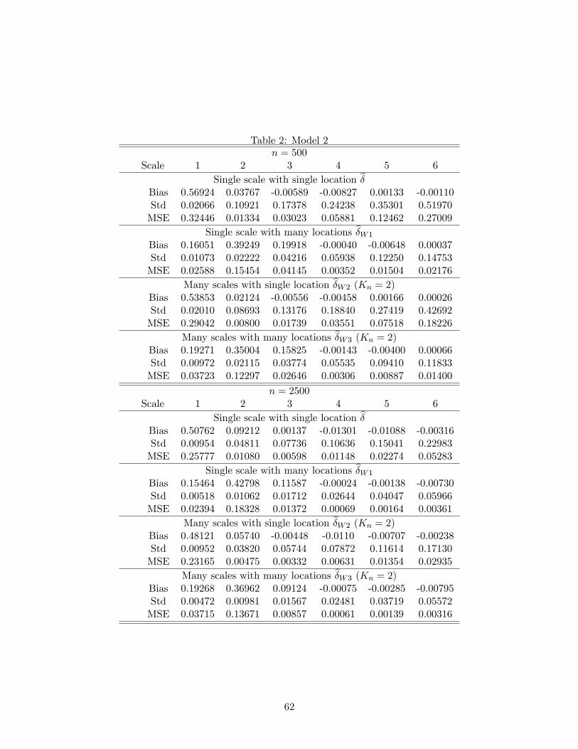
Table 2: Model 2n = 500

Scale 1 2 3 4 5 6

Single scale with single location b�Bias 0.56924 0.03767 -0.00589 -0.00827 0.00133 -0.00110Std 0.02066 0.10921 0.17378 0.24238 0.35301 0.51970MSE 0.32446 0.01334 0.03023 0.05881 0.12462 0.27009

Single scale with many locations b�W1

Bias 0.16051 0.39249 0.19918 -0.00040 -0.00648 0.00037Std 0.01073 0.02222 0.04216 0.05938 0.12250 0.14753MSE 0.02588 0.15454 0.04145 0.00352 0.01504 0.02176

Many scales with single location b�W2 (Kn = 2)Bias 0.53853 0.02124 -0.00556 -0.00458 0.00166 0.00026Std 0.02010 0.08693 0.13176 0.18840 0.27419 0.42692MSE 0.29042 0.00800 0.01739 0.03551 0.07518 0.18226

Many scales with many locations b�W3 (Kn = 2)Bias 0.19271 0.35004 0.15825 -0.00143 -0.00400 0.00066Std 0.00972 0.02115 0.03774 0.05535 0.09410 0.11833MSE 0.03723 0.12297 0.02646 0.00306 0.00887 0.01400

n = 2500Scale 1 2 3 4 5 6

Single scale with single location b�Bias 0.50762 0.09212 0.00137 -0.01301 -0.01088 -0.00316Std 0.00954 0.04811 0.07736 0.10636 0.15041 0.22983MSE 0.25777 0.01080 0.00598 0.01148 0.02274 0.05283

Single scale with many locations b�W1

Bias 0.15464 0.42798 0.11587 -0.00024 -0.00138 -0.00730Std 0.00518 0.01062 0.01712 0.02644 0.04047 0.05966MSE 0.02394 0.18328 0.01372 0.00069 0.00164 0.00361

Many scales with single location b�W2 (Kn = 2)Bias 0.48121 0.05740 -0.00448 -0.0110 -0.00707 -0.00238Std 0.00952 0.03820 0.05744 0.07872 0.11614 0.17130MSE 0.23165 0.00475 0.00332 0.00631 0.01354 0.02935

Many scales with many locations b�W3 (Kn = 2)Bias 0.19268 0.36962 0.09124 -0.00075 -0.00285 -0.00795Std 0.00472 0.00981 0.01567 0.02481 0.03719 0.05572MSE 0.03715 0.13671 0.00857 0.00061 0.00139 0.00316

62

Table 3: Model 3n = 500

Scale 1 2 3 4 5 6

Single scale with single location b�Bias 1.3147 0.40031 0.17508 0.03774 0.03576 -0.00841Std 0.02072 0.10775 0.17249 0.24849 0.34953 0.52059MSE 1.7290 0.17186 0.06040 0.06317 0.12345 0.27108

Single scale with many locations b�W1

Bias 0.72221 0.67465 0.26152 -0.01437 0.00140 0.00901Std 0.01081 0.02238 0.03728 0.06064 0.12690 0.14753MSE 0.52170 0.45565 0.06978 0.00388 0.01610 0.02184

Many scales with single location b�W2 (Kn = 2)Bias 1.2595 0.30005 0.11654 0.03105 0.01737 -0.01309Std 0.02025 0.08542 0.13085 0.18742 0.27159 0.42165MSE 1.5869 0.09732 0.03070 0.03609 0.07406 0.17796

Many scales with many locations b�W3 (Kn = 2)Bias 0.70405 0.58876 0.20586 -0.01022 0.00351 0.00749Std 0.00980 0.02070 0.03460 0.05743 0.09661 0.11894MSE 0.49579 0.34707 0.04357 0.00340 0.00934 0.01420

n = 2500Scale 1 2 3 4 5 6

Single scale with single location b�Bias 1.2660 0.40237 0.13346 0.05457 0.01173 0.01949Std 0.00919 0.04578 0.07474 0.10968 0.16162 0.21138MSE 1.6028 0.16400 0.02339 0.01500 0.02625 0.04506

Single scale with many locations b�W1

Bias 0.72128 0.69221 0.17167 -0.00142 0.00070 0.00087Std 0.00478 0.00975 0.01713 0.02711 0.03861 0.05751MSE 0.52027 0.47926 0.02976 0.00073 0.00149 0.00330

Many scales with single location b�W2 (Kn = 2)Bias 1.2097 0.29508 0.09356 0.03735 0.01369 0.01499Std 0.00893 0.03746 0.05788 0.08500 0.12059 0.16217MSE 1.4636 0.08847 0.01210 0.00862 0.01473 0.02652

Many scales with many locations b�W3 (Kn = 2)Bias 0.70351 0.59553 0.13510 -0.00097 0.00065 0.00077Std 0.00438 0.00910 0.01586 0.02480 0.03550 0.05481MSE 0.49494 0.35474 0.01850 0.0006 0.00126 0.00300

63

Table 4: Model 4n = 500

Scale 1 2 3 4 5 6

Single scale with single location b�Bias 0.76726 0.13214 0.04122 -0.00451 0.01112 -0.01362Std 0.02089 0.10759 0.17274 0.24254 0.35835 0.52279MSE 0.58913 0.02904 0.03154 0.05884 0.12853 0.27350

Single scale with many locations b�W1

Bias 0.46991 0.44709 0.17340 -0.00769 -0.00031 0.00466Std 0.01096 0.02238 0.03677 0.05917 0.11750 0.14873MSE 0.22094 0.20039 0.03142 0.00356 0.01380 0.02214

Many scales with single location b�W2 (Kn = 2)Bias 0.72995 0.09286 0.02400 -0.00127 0.00174 -0.01317Std 0.02038 0.08484 0.13091 0.18938 0.28215 0.43292MSE 0.53325 0.01582 0.01771 0.03586 0.07961 0.18759

Many scales with many locations b�W3 (Kn = 2)Bias 0.45927 0.39024 0.13675 -0.00567 0.00116 0.00395Std 0.010004 0.02078 0.03406 0.05531 0.09130 0.12020MSE 0.21103 0.15272 0.01986 0.00309 0.0083 0.01446

n = 2500Scale 1 2 3 4 5 6

Single scale with single location b�Bias 0.74038 0.13072 0.01623 0.00481 -0.00829 -0.00970Std 0.00872 0.04857 0.07493 0.09976 0.14984 0.21606MSE 0.54824 0.01944 0.00587 0.00997 0.02252 0.04677

Single scale with many locations b�W1

Bias 0.47196 0.45551 0.10940 0.00092 0.00017 -0.00286Std 0.00472 0.01058 0.01650 0.02731 0.03946 0.05732MSE 0.22277 0.20760 0.01224 0.00074 0.00155 0.00329

Many scales with single location b�W2 (Kn = 2)Bias 0.70192 0.08772 0.00947 -0.00099 -0.00900 -0.01215Std 0.00868 0.03806 0.05706 0.07918 0.11714 0.16592MSE 0.49277 0.00914 0.00334 0.00627 0.01380 0.02767

Many scales with many locations b�W3 (Kn = 2)Bias 0.46062 0.39143 0.08640 0.00062 -0.00052 -0.00235Std 0.00432 0.00970 0.01519 0.02541 0.03620 0.05276MSE 0.21219 0.15331 0.00769 0.00064 0.00131 0.00278

64