Embed Size (px)
Citation preview

This is page iPrinter: Opaque this
Categoricity
John Baldwin
January 6, 2004
This is page vPrinter: Opaque this

vi

This is page viiPrinter: Opaque this
Contents
1 Introduction 1
2 Combinatorial Geometries 3
3 Abstract Quasiminimality 5
4 Covers of the Multiplicative Group of Z 13
5 Abstract Elementary Classes 21
6 Non-definability of Well-order in Lω1,ω(Q) 27
7 Categoricity implies Completeness 317.1 Completeness . . . . . . . . . . . . . . . . . . . . . . . . . . 317.2 Arbitrarily Large Models . . . . . . . . . . . . . . . . . . . . 347.3 Few models in small cardinals . . . . . . . . . . . . . . . . . 36
8 A model in ℵ2 39
9 Galois types and Saturation 43
10 Homogeneity and Saturation 47
11 Galois Stability 53

viii Contents
12 Omitting types and Downward Categoricity 59
13 Atomic AEC 63
14 The ω1-order property 65
15 Independence in ω-stable Classes 67
16 Consequences of Excellence 75
17 Quasiminimal Sets in Excellent Classes 77
18 Two Cardinal Models and Categoricity Transfer 83
19 Demystifying Non-excellence 8719.1 The basic structure . . . . . . . . . . . . . . . . . . . . . . . 8719.2 k = 2, ℵ1-categoricity . . . . . . . . . . . . . . . . . . . . . 8919.3 k = 3, ℵ2-categoricity . . . . . . . . . . . . . . . . . . . . . 9019.4 Failure of Categoricity in 2ℵ1 . . . . . . . . . . . . . . . . . 9119.5 Failure of tameness . . . . . . . . . . . . . . . . . . . . . . 93
References 95
Index 100

This is page 1Printer: Opaque this
1Introduction
I will of course rewrite the introduction when the monograph is finished soit reflects what I ended up with not what I thought would end up with.But here are the aims now.
The following themes are interweaved.1. I want to expound Shelah’s categoricity theorem for Lω1,ω. Very
vaguely, I think of this as having two parts. a) Categoricity in enoughpowers implies excellence; b) excellence implies categoricity transfers.
Most of what is written on this line lies in part b). In order for a) +b) to yield categoricity in a small initial segment of the cardinals yieldscategoricity in all cardinals, our analysis of b) cannot assume the existenceof arbitrarily large models. We motivate the exposition by doing Zilber’sspecial case of quasiminimal excellence and connecting it with his conjec-tures on complex exponentiation. But the natural axiomatization of Zilber’sclasses are not in Lω1,ω but in Lω1,ω(Q). So we would like to have the re-sults for Lω1,ω(Q). I don’t believe this can be done with out much moresophisticated techniques, e.g. λ-frames of [36, 35, 34]; they are beyond thescope of these notes. But the basic properties of abstract elementary classesare developed so as to prepare for study of e.g. frames. An unwritten chap-ter will connect Lω1,ω(Q) with AEC’s. At the moment we only notice thatthe first two or three obvious ways to translate are wrong.
Eventually, we will do a).2. A different perspective is the conjecture that for reasonably well-
behaved classes, categoricity should be either eventually true or eventuallyfalse. Here we introduce the notion of AEC and prove the presentation the-orem and categoricity implies stability Some of the results in this general
2 1. Introduction
framework are applied in the Lω1,ω-case. For this part, the assumption ofarbitrarily large models is entirely reasonable. Again we expound some sim-pler versions of this result (using strong amalgamation hypotheses). Thistoo leads to λ-frames.
3. In the midst of this I intend to describe the taxonomy of infinitary cat-egoricity - the relations among various infinitary languages, homogeneousmodel theory, excellent classes, AEC etc.
I don’t organize around techniques (as Keisler did) but there are sev-eral techniques that eventually are expounded; combinatorial geometries,EM-models and then the introduction of splitting to get an independencerelation generalizing a combinatorial geometry.
The only quoted material is very elementary model theory (say a smallpart of Marker’s book), Morley’s omitting types theorem, and two or threetheorems from the Keisler book including Lopez-Escobar.
In addition to the fundamental papers of Shelah, this exposition dependsheavily on various works by Grossberg and Lessmann.

This is page 3Printer: Opaque this
2Combinatorial Geometries
Definition 2.1 A pregeometry is a set G together with a dependence re-lation
cl : P(G) → P(G)
satisfying the following axioms.A1. cl(X) =
⋃{cl(X ′) : X ′ ⊆fin X}A2. X ⊆ cl(X)A3. cl(cl(X)) = cl(X)A4. If a ∈ cl(Xb) and a 6∈ cl(X), then b ∈ cl(Xa).If points are closed the structure is called a geometry.
Definition 2.2 A geometry is homogeneous if for any closed X ⊆ G anda, b ∈ G−X there is a permutation of G which preserves the closure relation(i.e. an automorphism of the geometry) which fixes X pointwise and takesa to b.
Exercise 2.3 If G is a homogeneous geometry, X, Y are maximally inde-pendent subsets of G, there is an automorphism of G taking X to Y .
Definition 2.4 1. The structure M is strongly minimal strongly min-imal if every first order definable subset of any elementary extensionM ′ of M is finite or cofinite.
2. The theory T is strongly minimal if it is the theory of a stronglyminimal structure.
3. a ∈ acl(X) if there is a first order formula with finitely solutions overX which is satisfied by a.

4 2. Combinatorial Geometries
Definition 2.5 Let X,Y be subsets of a structure M . An elementary iso-morphism from X to Y is 1-1 map from X onto Y such that for every firstorder formula φ(v), M |= φ(x) if and only if M |= φ(fx).
Exercise 2.6 Find X,Y subsets of a structure M such that X and Y areisomorphic but not elementarily isomorphic.
Exercise 2.7 Let X,Y be subsets of a structure M . If f takes X to Y isan elementary isomorphism, f extends to an elementary isomorphism fromacl(X) to acl(Y ).
Exercise 2.8 Show a complete theory T is strongly minimal if and only ifit has infinite models and
1. algebraic closure induces a pregeometry on models of T ;
2. any bijection between acl-bases for models of T extends to an isomor-phism of the models.
Exercise 2.9 A strongly minimal theory is categorical in any uncountablecardinality.

This is page 5Printer: Opaque this
3Abstract Quasiminimality
Since I have and will use the term:
Definition 3.1 A structure M is κ-sequence homogeneous if for any a,b ∈M of length less than κ, if (M, a) ≡ (M,b) then for every c, there exists dsuch that (M, ac) ≡ (M,bd).
An abstract quasiminimal class is a class of structures that satisfy thefollowing five conditions, which we expound leisurely.
Assumption 3.2 (Condition I) Let K be a class of L-structures whichadmit a monotone idempotent closure operation cl taking subsets of M ∈ Kto substructures of M such that cl has finite character.
Strictly speaking, we should write clM (X) rather than cl(X) but we willomit the M where it is clear from context.
Definition 3.3 Let A be a subset of H, H ′ ∈ K. A map from X ⊂ H −Ato X ′ ⊂ H ′ − A is called a partial A-monomorphism if its union with theidentity map on A preserves quantifier free formulas.
Freqently, but not necessarily we will have A = G which is in K.
Definition 3.4 Let Ab ⊂ M and M ∈ K. The (quantifier-free) typeof b over A in M , written tpqf (b/A;M) ( tpqf (b/A; M)), is the set of(quantifier-free) first-order formulas with parameters from A true of b inM .
Exercise 3.5 Why is M a parameter in Definition 3.4?

6 3. Abstract Quasiminimality
Exercise 3.6 Let Ab ⊂ M , Ab′ ⊂ M ′ with M,M ′ ∈ bK. Show there isa partial A-monomorphism taking a′ to b′ if and only if tpqf (b/A;M) =tpqf (b′/A; M ′).
The next assumption connects the geometry with the structure on mem-bers of K.
Assumption 3.7 (Condition II) Let G ⊆ H, H ′ ∈ K with G empty orin K.
1. If f is a bijection between X and X ′ which are separately cl-independent (over G) subsets of H and H ′ then f is a partial G-monomorphism.
2. If f is a partial G-monomorphism from H to H ′ taking X ∪ {y} toX ′ ∪ {y′} then y ∈ cl(XG) iff y′ ∈ cl(X ′G).
Condition 3.7.2) has an a priori unlikely strength: quantifier free formulasdetermine the closure; in practice, the language is specifically expanded toguarantee this condition. Part 2 of Assumption 3.7 implies that each Mwith G ⊆ M ∈ K is finite sequence homogeneous over G.
Assumption 3.8 (Condition III : ℵ0-homogeneity over models)If f is a partial G-monomorphism from H to H ′ with finite domain Xthen for any y ∈ H there is y′ in an extension H ′′ ∈ K of H ′ such thatf ∪ {〈y, y′〉} extends f to a partial G-monomorphism.
If H and H ′ have finite dimension, we might need to extend H ′. Alter-native formulations would be to only make the assumption for y ∈ clH(X)or to require that H ′ have infinite dimension.
Question 3.9 Let a, b be independent over the empty set. Suppose fa, fb
map cl(a) (cl(b)) into a K-structure H. Is fa ∪ fb a monomorphism? (Weprove below that the answer is yes assuming exchange; is exchange neces-sary?
Definition 3.10 We say a closure operation satisfies the countable closurecondition if the closure of a countable set is countable.
We easily see:
Lemma 3.11 Suppose Assumptions I, II, and III are satisfied by cl on anuncountable structure M ∈ K that satisfies the countable closure condition.
1. For any finite set X ⊂ M , if a, b ∈ M − cl(X), a, b realize the sameLω1,ω type over X.
2. Every Lω1,ω definable subset of M is countable or cocountable. Thisimplies that a ∈ cl(X) iff it satisfies some φ over X, which has onlycountably many solutions.

3. Abstract Quasiminimality 7
Proof. Condition 1) follows directly from Conditions II and III (Assump-tion 3.7 and Assumption 3.8) by constructing a back and forth. To seecondition 2), suppose both φ and ¬φ had uncountably many solutions withφ defined over X. Then there are a and b satisfying φ and ¬φ respectivelyand neither is in cl(X); this contradicts 1).
The ω-homogeneity yields by an easy induction:
Lemma 3.12 Suppose Assumptions I II and III hold. Let G ∈ K be count-able and suppose G ⊂ H1,H2 ∈ K.
1. If X ⊂ H−G, X ′ ⊂ H−G are finite and f is a G-partial monomor-phism from X to X ′ then f extends to a G-partial monomorphismfrom clH(GX) to clH′(GX ′).
2. If X is independent set of cardinality at most ℵ1, and f is a G-partial monomorphism from X to X ′ then f extends to a G-partialmonomorphism from clH(GX) to clH′(GX ′).
Proof. The first statement is immediate from homogeneity. The secondfollows by induction from the first (by replacing G by cl(GX0) for X0 acountable initial segment of X). ¤3.12
For algebraic closure the cardinality restriction on X is unnecessary. Wewill have to add Assumption 3.8 to remove the restriction in excellentclasses.
Assumption 3.13 (Condition IV) cl satisfies the exchange axiom: y ∈cl(Xx)− cl(X) implies x ∈ cl(Xy).
Zilber omits exchange in the fundamental definition but it arises in thenatural contexts he considers so we make it part of quasiminimal excellence.Note however that the examples of first order theories with finite Morleyrank greater than 1 (e.g. [2]) fail exchange.
In the following definition it is essential that ⊂ be understood as propersubset.
Definition 3.14 1. For any Y , cl−(Y ) =⋃
X⊂Y cl(X).
2. We call C (the union of) an n-dimensional cl-independent system ifC = cl−(Z) and Z is an independent set of cardinality n.
To visualize a 3-dimensional independent system think of a cube with theempty set at one corner A and each of the independent elements z0, z1, z2 atthe corners connected to A. Then each of cl(zi, zj) for i < j < 3 determinesa side of the cube: cl−(Z) is the union of these three sides; cl(Z) is theentire cube.
Assumption 3.15 (Condition V) Let G ⊆ H, H ′ ∈ K with G emptyor in K. Suppose Z ⊂ H − G is an n-dimensional independent system,

8 3. Abstract Quasiminimality
C = cl−(Z), and X is a finite subset of cl(Z). Then there is a finite C0
contained in C such that: for every G-partial monomorphism f mappingX into H ′, for every G-partial monomorphism f1 mapping C into H ′, iff ∪ (f1 ¹ C0) is a G-partial monomorphism, f ∪ f1 is also a G-partialmonomorphism.
We can rephrase the conclusion as for any a ∈ cl(Z) there is a finiteCa ⊆ C such that tpqf (a/Ca;H) implies tpqf (a/C; H).
Thus Condition IV, which is the central point of excellence, asserts (fordimension 3) that the type of any element in the cube over the union of thethree given sides is determined by the type over a finite subset of the sides.The ‘thumbtack lemma’ of Chapter 4 verifies this condition in a specificalgebraic context. Here is less syntactic version of Assumption 3.8
Definition 3.16 We say M ∈ K is prime over the set X ⊂ M if everypartial monomorphism of X into N ∈ K extends to a monomorphism ofM into N .
Remark 3.17 Note that in first order logic this corresponds to ‘alge-braically prime’ rather than ‘elementarily prime’. In the first order con-text algebraically prime is a notoriously unstable (in a nontechnical sense)concept.
Lemma 3.18 Let G ⊆ H, H ′ ∈ K with G empty or in K and countable.Suppose Z ⊂ H −G is an n-dimensional independent system, C = cl−(Z),then cl(Z) ⊆ H is prime over C.
Proof. Fix an embedding f from C into H ′ containing G. We must extendf to f mapping cl(Z) into H ′. We can enumerate cl(X) as ai : i < ω. LetAn denote {ai : i < n}. Now define by induction an increasing sequenceof finite sets Bn : n < ω such that tpqf (An/Bn;H) implies tpqf (An/C; H)and
⋃n<ω Bn = C. Now, using only part of Lemma 3.12 1), construct an
increasing family of maps fn with the domain of fn = An ∪ Bn. Then theunion of these functions is the required embedding. ¤3.18
Theorem 3.19 Let K be a quasiminimal excellent class and supposeH, H ′ ∈ K satisfy the countable closure condition. Let A,A′ be cl-independent subsets of H, H ′ with cl(A) = H, cl(A′) = H ′, respectively,and ψ a bijection between A and A′. Then ψ extends to an isomorphismof H and H ′.
Suppose further, that some model of K contains an infinite cl-independent set. Then the class of K-structures which satisfy the countableclosure condition is categorical in every uncountable cardinality.
The remainder of this section is devoted to the proof of Theorem 3.19
Notation 3.20 Fix a countable subset A0 and write A as the disjointunion of A0 and a set A1; without loss of generality, we can assume ψ

3. Abstract Quasiminimality 9
is the identity on clH(A0) and work over G = clH(A0). We may writecl∗(X) to abbreviate cl(A0X).
Lemma 3.21 Suppose X, Y are subsets of A1. Suppose b ∈ cl(A0X) andc ∈ cl(A0Y ) and p(b, c,g) for some quantifier-free type q (over g ∈ G).Then there is a map π into cl(A0Y ) whose domain includes bcg, that fixescg, and such that p(bπcg) holds.
Proof. Choose finite A∗ ⊂ A0 such that g ∈ cl(A∗), b ∈ cl(A∗X), andc ∈ cl(A∗Y ). Let G0 = cl(A∗Y ). Extend the identity map on G0 to π1 withdomain G0X by mapping X−Y into A0−(A∗Y ). By Assumption 3.7 .1, π1
is a partial G0-monomorphism. By Lemma 3.12 π1 extends to a partial G0-monomorphism π from cl(A∗XY ) into cl∗(Y ). Clearly π has the requiredproperty. ¤3.21
Lemma 3.22 Suppose X,Y are subsets of A1 and that ψX and ψY areeach partial G-monomorphisms from H into H ′ with domψX = cl(A0X)and domψY = cl(A0Y ) that agree on cl(A0X) ∩ cl(A0Y ). Then ψX ∪ ψY
is a partial G-monomorphism.
Proof. By Lemma 3.12 there is a partial G-monomorphism ψXY whichextends ψX and maps cl∗(XY ) into H ′. Another partial map on cl∗(X) ∪cl∗(Y ) is given by ψX ∪ ψY . It suffices to show that for any b ∈ cl∗(X),g ∈ G and c ∈ cl∗(Y ) and any quantifier free R, H ′ |= R(ψX(b), ψXY (c),g)if and only if H ′ |= R(ψX(b), ψY (c),g). So we are finished if we apply thefollowing lemma to H ′. To apply the Lemma, note that ψXY ◦ ψ−1
Y is apartial G-monomorphism taking ψY (c) to ψXY (c).
Lemma 3.23 Let X, Y, Y ′ ⊆ A1. Let b ∈ cl(A0X), c ∈ cl(A0Y ), andc′ ∈ cl(A0Y
′). Suppose f is a partial G-monomorphism taking c to c′, thenf is a partial cl∗(X) monomorphism.
Proof. If not there exists b ∈ cl∗(X) and g ∈ G and a quantifier freeR such that R(b, c,g) ∧ ¬R(b, c′,g). Now apply Lemma 3.21, to obtaina map π into cl(A0Y Y ′) which fixes c, c′,g and such that R(bπ, c,g) ∧¬R(bπ, c′,g). This contradicts that c, c′ are partially isomorphic over G.¤3.23
¤3.22
We have by straightforward induction.
Corollary 3.24 Suppose 〈Xi : i < m〉 are subsets of A and that each ψXi
is a partial G-monomorphisms from H into H ′ with dom ψXi = cl(A0Xi)and that for any i, j, ψXi and ψXj agree whenever both are defined. ThenψX ∪ ψY is a partial G-monomorphism.
Proof of Theorem 3.19. Note that H = limX⊂A;|X|<ℵ0 cl(X). We havethe obvious directed system on {cl(X) : X ⊂ A; |X| < ℵ0}. So the theoremfollows immediately if for each finite X we can choose ψX : cl(X) → H ′ so
10 3. Abstract Quasiminimality
that X ⊂ Y implies ψX ⊂ ψY . We prove this by induction on |X|. Suppose|Y | = n + 1 and we have appropriate ψX for |X| < n + 1. We will provetwo statements by induction.
1. ψ−Y : cl−(Y ) → H ′ defined by ψ−Y =⋃
X⊂Y ψX is a monomorphism.
2. ψ−Y extends to ψY defined on cl(Y ).
The first step is done by induction using Corollary 3.24 with the X ⊂ Ywith |X| = n as the Xi. The exchange axiom is used to guarantee that themaps ψX agree where more than one is defined. The second step followsby Lemma 3.18.
We have shown that the isomorphism type of a structure in K withcountable closures is determined by the cardinality of a basis for the geom-etry. If M is an uncountable model in K that satisfies the countable closurecondition, the size of M is the same as its dimension so there is at mostone model in each uncountable cardinality which has countable closures. Itremains to show that there is at least one.
Lemma 3.25 If there is an H ∈ K which contains an infinite cl-independent set, then there are members of K of arbitrary cardinality whichsatisfy the countable chain condition.
Proof. Let L∗ be a countable fragment of Lω1,ω containing the sentenceaxiomatizing K and the formulas defining independence. Let X be a count-able independent set of H, H1 the closure of Xa where a is independentfrom X and let H0 = clH1(X). Note that H0 ≺L∗ H1 by a back andforth. Since cl is L∗-definable H0 = clH0(X). So we have a model whichis isomorphic to a proper L∗-elementary extension. As in [42] since allmembers of K with countably infinite dimension are isomorphic, one canconstruct a continuous L∗-elementary increasing chain of members of Kfor any α < ℵ1. Thus we get a model of power ℵ1. Note that each Hℵ1 hascountable closures since the closure of any countable set is contained in amodel isomorphic to Hω. Continue the same construction, to construct amodel of power ℵ2. Now we use the categoricity established above to passlimit ordinals. Since the chain is L∗-elementary, each Hα ∈ K. Now we getarbitrarily large models using the categoricity at κ to construct a model ofpower κ+. ¤3.19
Note that a sentence ψ can define a quasiminimal excellent class withoutbeing ℵ0-categorical. But we could extend ψ to ψ′ - the Scott sentence ofthe model with countably infinite cl-dimension and attain ℵ0-categoricity.
The following corollary seems to rely on the categoricity argument. Thekey is Condition II (??) and for countable G it follows from Lemma 3.12.But in general we use Theorem 3.19.
Corollary 3.26 Let K be a quasiminimal excellent class, with G ⊂ H, H ′
all in K. If a ∈ H, a′ ∈ H ′ realize the same quantifier free type over G (i.e.

3. Abstract Quasiminimality 11
there is a G-monomorphism taking a to a′) then there is a K-isomorphismfrom cl(Ga) onto cl(Ga′).
Thus (G, a, H) and (G, a′,H ′) realize the same Galois type.
Exercise 3.27 Define a notion of almost quasiminimality analogous toalmost strong minimality and prove that almost quasiminimal classes arecategorical in all powers ([44]).
Question 3.28 Zilber’s proof of Theorem 3.19 is considerably more com-plicated. I think this is because he does not assume exchange. How wouldyou modify the argument here to avoid the use of exchange?

12 3. Abstract Quasiminimality

This is page 13Printer: Opaque this
4Covers of the Multiplicative Group of Z
The first approximation to a quasiminimal axiomatization of complex ex-ponentiation considers short exact sequences of the following form.
0 → Z → H → F ∗ → 0. (4.1)
H is a torsion-free divisible abelian group (written additively), F is analgebraically closed field, and exp is the homomorphism from (H, +) to(F ∗, ·), the multiplicative group of F . We can code this sequence as astructure for a language L:
(H, +, E, S),
where E(h1, h2) iff exp(h1) = exp(h2) and we pull back sum by thedefining H |= S(h1, h2, h3) iff F |= exp(h1) + exp(h2) = exp(h3). Thus Hnow represents both the multiplicative and additive structure of F .
To guarantee Assumption 3.7.2 we expand the language further. Letexp : H 7→ F ∗. For each affine variety over Q, V (x1, . . . xn), weadd a relation symbol V interpreted by H |= V (h1, . . . , hn) iff F |=V (exp(h1), . . . , exp(hn)). This includes the definition of S mentioned above;we have some fuss to handle the pullback of relations which have 0 in theirrange.
Lemma 4.1 There is an Lω1,ω-sentence Σ such that there is a 1-1 corre-spondence between models of Σ and sequences (4.1).

14 4. Covers of the Multiplicative Group of Z
The sentence asserts first that the quotient of H by E with + corre-sponding to × and S to + is an algebraically closed field. We use Lω1,ω
to guarantee the kernel is 1-generated. This same proviso insures that therelevant closure condition has countable closures.
Definition 4.2 For X ⊂ H |= Σ,
cl(X) = exp−1(acl(exp(X))
where acl is the field algebraic closure in F .
Using this definition of closure the key result of [43] asserts:
Theorem 4.3 Σ is quasiminimal excellent with the countable closure con-dition and categorical in all uncountable powers.
Our goal is this section is to prove this result modulo one major algebraiclemma. We will frequently work directly with the sequence (1) rather thanthe coded model of Σ. Note that (1) includes the field structure on F .That is, two sequences are isomorphic if there are commuting maps H toH ′ etc. where the first two are group isomorphisms but the third is a fieldisomorphism.
It is easy to check that Conditions I and IV and countable closures aresatisfied: cl gives a combinatorial geometry such that the countable closureof countable sets is countable. We need more notation about the divisibleclosure (in the multiplicative group of the field to understand the remainingconditions.
Definition 4.4 By a divisibly closed multiplicative subgroup associatedwith a ∈ C∗, aQ, we mean a choice of a multiplicative subgroup containinga and isomorphic to the additive group Q.
Definition 4.5 We say b1m1 ∈ b
Q1 , . . . b
1m
` ∈ bQ` ⊂ C∗, determine the iso-
morphism type of bQ1 , . . . b
Q` ⊂ C∗ over the subfield k of C if given sub-
groups of the form cQ1 , . . . c
Q` ⊂ C∗ and φm such that
φm : k(b1m1 . . . b
1m
` ) → k(c1m1 . . . c
1m
` )
is a field isomorphism it extends to
φ∞ : k(bQ1 , . . . bQ` ) → k(cQ1 , . . . c
Q` ).
To see the difficulty consider the following example.
Example 4.6 Let a1 and a2 be linearly independent over Q complex num-bers such that (a1−1)2 = a2. Suppose φ, which maps Q(a1, a2) to Q(c1, c2),is a field isomorphism. φ does not extend to an isomorphism of their divis-ible hulls, we might have a1 − 1 =
√a2 but c1 − 1 = −√c2.

4. Covers of the Multiplicative Group of Z 15
As in Lecture 3, for G a subgroup of H, H ′ and H,H ′ |= Σ, a partialfunction φ on H is called a G-monomorphism if it preserves L-quantifierfree formulas with parameters from G.
Fact 4.7 Suppose b1, . . . b` ∈ H and c1, . . . c` ∈ H ′ are each linearly in-dependent sequences (from G) over Q. Let G be the subfield generatedby exp(G). If G(exp(b1)Q, . . . exp(b`)Q) ≈ G(exp(c1)Q, . . . exp(c`)Q) asfields, then mapping bi to ci is a G-monomomorphism preserving each va-riety V .
Proof. Let G ⊂ H and suppose rational qi, ri are rational numbers, hi ∈H −G, gi ∈ G. Then
H |= V (q1b1, . . . q`b`, r1g1, . . . rmgm)
iffH |= V (exp(q1b1), . . . exp(q`b`), exp(r1g1), . . . exp(rmgm))
iffG(exp(b1)Q, . . . exp(b`)Q, exp(g1)Q, . . . exp(gm)Q)
|= V (exp(q1b1), . . . exp(q`b`), exp(r1g1), . . . exp(rmgm)).
From this fact, it is straightforward to see that Condition II in the def-inition of quasiminimal excellence holds. For II.i) we need that there isonly one type of a closure-independent sequence. But Fact 4.7 implies thatfor b ∈ H to be closure independent, the associated exp(b) must be al-gebraically independent and of course there is a unique type of an alge-braically independent sequence. For II.ii) holds since added to language ofΣ predicates for the pull-back of all quantifier-free relations on the field F .(Zilber doesn’t do this.)
For Condition III and the excellence condition we need an algebraic re-sult. In the following,
√1 denotes the subgroup of roots of unity. We call
this result the thumbtack lemma based on the following visualization ofKitty Holland. The various nth roots of b1, . . . bm hang on threads from thebi. These threads can get tangled; but the theorem asserts that by stickingin a finite number of thumbtacks one can ensure that the rest of stringsfall freely. The proof involves the theory of fractional ideals of numberfields, Weil divisors, and the normalization theorem. For a1, . . . ar in C, wewrite gp(a1, . . . ar) for the multiplicative subgroup generated by a1, . . . ar.The following general version of the theorem is applied for various sets ofparameters to prove quasiminimal excellence.
In the following Lemma we write√
1 for the group of roots of unity. Ifany of the Li are defined, the reference to
√1 is redundant. We write gp(a)
for the multiplicative subgroup generated by a.
Remark 4.8 Let k be an algebraically closed subfield in C and let a ∈ C−k. A field theoretic description of the relation of a to k arises by taking the

16 4. Covers of the Multiplicative Group of Z
irreducible variety over k realized by a. a is a generic realization of varietygiven by a finite conjunction φ(x,b) of polynomials generating the idealin k[x] of those polynomials which annihilate a. From a model theoreticstandpoint we can say, choose b so that the type of a/k is the uniquenonforking extension of tp(a/b). We use the model theoretic formulationbelow. See [1], page 39.
Theorem 4.9 (thumbtack lemma) [43]Let P ⊂ C be a finitely generated extension of Q and L1, . . . Ln alge-
braically closed subfields of the algebraic closure P of P . Fix multiplicatively
divisible subgroups aQ1 , . . . a
Qr with a1, . . . ar ∈ P and b
Q1 , . . . b
Q` ⊂ C∗. If
b1 . . . b` are multiplicatively independent over gp(a1, . . . ar) ·√
1 ·L∗1 · . . . L∗nthen for some m b
1m1 ∈ b
Q1 , . . . b
1m
` ∈ bQ` ⊂ C∗, determine the isomorphism
type of bQ1 , . . . b
Q` over P (L1, . . . Ln,
√1, aQ1 , . . . a
Qr ).
Lemma 4.10 Condition III of quasiminimal excellence holds.
Proof. We must show: If G |= Σ and f is a partial G-monomorphism fromH to H ′ with finite domain X = {x1, . . . , xr} then for any y ∈ H there is y′
in some H ′′ with H ′ ≺K H ′′ such that f ∪ {〈y, y′〉} extends f to a partialG-monomorphism. Since G |= Σ, exp(G) is an algebraically closed field.For each i, let ai denote exp(xi) and similarly for x′i, a
′i. Choose a finite
sequence d ∈ exp(G) such that the sequence (a1, . . . ar) is independent (inthe forking sense) from exp(G) over d and tp(a1, . . . ar)/d) is stationary.Now we apply the thumbtack lemma. Let P0 be Q(d). Let n = 1 and L1 bethe algebraic closure of P0. We set P0(d, a1, . . . ar) as P . Take b1 as exp(y)and set ` = 1.
Now apply Lemma 4.9 to find m so that b1m1 determines the algebraic type
of (b1)Q over L1(aQ1 , . . . a
Qr ) = P0(L1, a
Q1 , . . . a
Qr ). Let f denote the map f
induces from H to H ′ over G. Choose b′11m to satisfy the quantifier free field
type of f(tp(b1m1 /L1(a
Q1 , . . . a
Qr ). Now by Lemma 4.9, f extends to field iso-
morphism between L1(aQ1 , . . . a
Qr , b
Q1 )) and L1((a′1)
Q, . . . (a′r)Q, (b′1)
Q).Since the sequence a1, . . . ar) is independent (in the forking sense) from
exp(G) over L1, we can extend this map to take exp(G)(aQ1 , . . . aQr , b
Q1 )
to exp(G)((a′1)Q, . . . (a′r)Q, (b′1)
Q) and pull back to find y′; this suffices byFact 4.7.
¤4.10
Note there is no claim that y′ ∈ H ′ and there can’t be.One of the key ideas discovered by Shelah in the investigation of non-
elementary classes is that in order for types to be well-behaved one mayhave to make restrictions on the domain. (E.g., we may be able to amal-gamate types over models but not arbitrary types.) This principle is illus-trated by the following definition and result of Zilber.

4. Covers of the Multiplicative Group of Z 17
Definition 4.11 C ⊆ F is finitary if C is the union of the divisible closure(in C∗) of a finite set and finitely many algebraically closed fields.
Now we establish Condition IV, excellence. Note that this is a strongercondition than excellence since there is no independence requirement onthe Gi.
Lemma 4.12 Let G1, . . . Gn ⊂ H all be models of Σ and suppose eachhas finite cl-dimension. If h1, . . . h` ∈ G− = cl(G1 ∪ . . . Gn) then there isfinite set A ⊂ G− such that any φ taking h1, . . . , h` into H which is anA-monomorphism is also a G−-monomorphism.
Let Li = exp(Gi) for i = 1, . . . , n; bqj = exp(qhj) for j = 1, . . . , ` and
q ∈ Q. We may assume the hi are linearly independent over the vector spacegenerated by the Gi; this implies the bi are muliplicatively independent overL∗1 ·L∗2 · . . . L∗n. Now apply the thumbtack lemma with r = 0. This gives an
m such that the field theoretic type of b1m1 , . . . , b
1m
` determines the quantifierfree type of (h1, . . . , h`) over G−. So we need only finitely many parametersfrom G− and we finish.
To prove the following result, apply the thumbtack lemma with the Li
as the fields and the ai as the finite set.
Corollary 4.13 Any almost finite n-type over a finitary set is a finite n-type.
Since we have established all the conditions for quasiminimal excellence,we have proved Theorem 4.3.
Keisler[16] proved Morley’s categoricity theorem for sentences in Lω1,ω,assuming that the categoricity model was ℵ1-homogeneous. This theoremis the origin of the study of homogeneous model theory which is well ex-pounded in e.g. [4]. We give two examples showing the homogeneity doesnot follow from categoricity. Marcus [24] showed:
Fact 4.14 There is a first order theory T with a prime model M such that
1. M has no proper elementary submodel.
2. M contains an infinite set of indiscernibles.
Exercise 4.15 Show that the Lω1,ω-sentence satisfied only by atomic mod-els of the theory T in Fact 4.14 has a unique model.
Example 4.16 Now construct an Lω1,ω-sentence ψ whose models are par-titioned into two sets; on one side is an atomic model of T , on the otheris an infinite set. Then ψ is categorical in all infinite cardinalities but nomodel is ℵ1-homogeneous because there is a countably infinite maximal in-discernible set.

18 4. Covers of the Multiplicative Group of Z
Now we see that the example of this chapter has the same inhomogeneityproperty.
Consider the basic diagram:
0 → Z → H → F ∗ → 0. (4.2)
Let a be a transcendental number in F ∗. Fix h with exp(h) = a anddefine an = exp h
n +1 for each n. Now choose hn so that exp(hn) = an. LetXr = {hi : i ≤ r}. Note that am = a
1m + 1 where we have chosen a specific
mth root.
Claim 4.17 pr = tp(h/Xr) is a principal type.
Proof. We make another application of the thumbtack Lemma 4.9 withQ(exp(span(Xr)) as P , a1, . . . ar as themselves, all Li are empty, and a asb1. By the lemma there is an m such that a
1m determines the isomorphism
type of aQ over P (aQ1 , . . . aQr ). That is if φm is the minimal polynomial of
a1m over P , (∃y)φm(y) ∧ ym = x generates tp(a/ exp(span(Xr))). Pulling
back by Lemma 4.7, we see tp(h/Xr) is principal and even complete forLω1,ω. In particular, for any m′ ≥ m, any two m′th roots of a have thesame type over exp(Xr). But for sufficiently large r, one of these m′throots is actually in Xr so tp(a/Xr) does not imply p = tp(a/X) for anyX. That is, tp(a/X) is not implied by its restriction to any finite set. Andby Lemma 4.7 this implies tpω1,ω(h/X) is not implied by its restriction toany finite set.
Now specifically to answer the question of Keisler [16], page 123, we needto show there is a sentence ψ in a countable fragment L∗ of Lω1,ω suchthat ψ is ℵ1-categorical but has a model with is not (ℵ1, L
∗)-homogeneous.Fix L∗ as a countable fragment containing the categoricity sentence for‘covers’. We have shown no formula of Lω1,ω (let alone L∗) with finitelymany parameters from X implies p. By the omitting types theorem for L∗,there is a countable model H0 of ψ which contains an L∗-equivalent copyX ′ of X and omits the associated p′. By categoricity, H0 imbeds into H.But H also omits p′. As, if h′ ∈ H, realizes p′, then exp(h′) ∈ acl(X ′) ⊆ H0
so since the kernel of exp is standard, h′ ∈ H0, contradiction. Thus thetype p′ cannot be realized so H is not homogeneous.
USED?
Definition 4.18 1. Let V be an irreducible variety over C ⊆ F . Thesequence associated with V over C is a sequence
{V 1m : m ∈ ω}

4. Covers of the Multiplicative Group of Z 19
such that V 1 = V and for any m,n ∈ ω, raising to the mth powermaps V
1nm to V
1n .
2. If V ′ ⊆ V are varieties over C, the pair
τ = (V − V ′, {V 1m : m ∈ ω})
is called an almost finite n-type over C.
3. Zilber calls a principal type given by a difference of varieties V − V ′
a finite n-type over C.
Sketch of Proof of Theorem 4.3. Another application of the thumb-tack lemma gives directly the homogeneity conditions of Condition III (As-sumption 3.8). Exchange, ( Assumption 3.13) , is immediate from the defini-tion of closure (4.2). Finitary sets are more general than the n-dimensionalindependent systems in the definition of quasiminimal excellence, since thesubsets don’t have to be independent. So if X is a sequence associated witha variety V over an n-dimensional independent system C, Corollary 4.13allows us to reduce X to a formula over a finite set yielding Excellence (As-sumption 3.15). So we finish by Theorem 3.19; the quasimimimal excellenceimplies categoricity.

20 4. Covers of the Multiplicative Group of Z

This is page 21Printer: Opaque this
5Abstract Elementary Classes
‘Non-elementary classes’ is a general term for any logic other than firstorder. Some of the most natural extensions of first order logic arise byallowing conjunctions of various infinite lengths or cardinality quantifiers.In this chapter we introduce a precise notion of ‘abstract elementary class’AEC which generalizes some of these logics. In this monograph we pursue adual track of proving certain result for general AEC and some for very spe-cific logics, especially Lω1,ω and Lω1,ω(Q). In this chapter we introduce thesemantic notion of an AEC and prove a surprising syntactic representationtheorem for such classes.
When Jonsson generalized the Fraisse construction to uncountable car-dinalities [13, 14], he did so by describing a collection of axioms, whichmight be satisfied by a class of models, that guaranteed the existence ofa homogeneous-universal model; the substructure relation was an integralpart of this description. Morley and Vaught [26] replaced substructure byelementary submodel and developed the notion of saturated model. Shelah[38, 39] generalized this approach in two ways. He moved the amalgamationproperty from a basic axiom to a constraint to be considered. (But this wasa common practice in universal algebra as well.) He made the substructurenotion a ‘free variable’ and introduced the notion of an Abstract Elemen-tary Class: a class of structures and a ‘strong’ substructure relation whichsatisfied variants on Jonsson’s axioms. To be precise
Definition 5.1 A class of L-structures, (K,≺K ), is said to be an abstractelementary class: AEC if both K and the binary relation ≺K are closedunder isomorphism and satisfy the following conditions.

22 5. Abstract Elementary Classes
• A1. If M ≺K N then M ⊆ N .
• A2. ≺K is a partial order on K.
• A3. If 〈Ai : i < δ〉 is ≺K -increasing chain:
1.⋃
i<δ Ai ∈ K;2. for each j < δ, Aj ≤
⋃i<δ Ai
3. if each Ai ≺K M ∈ K then⋃
i<δ Ai ≤ M .
• A4. If A,B, C ∈ K, A ≺K C, B ≺K C and A ⊆ B then A ≺K B.
• A5. There is a Lowenheim-Skolem number κ(K) such that if A ⊆B ∈ K there is a A′ ∈ K with A ⊆ A′ ≺K B and |A′| < κ(K).
Property A5 is sometimes called the coherence property and sometimes‘the funny axiom’. Perhaps best is the Tarski-Vaught property since it easilyseen to follow in the first order case as an application the Tarski-Vaught testfor elementary submodel. However, Shelah sometimes uses ‘Tarski-Vaught’for the union axioms.
Exercise 5.2 Show the class of well-orderings with ≺K taken as endextension satisfies the first four properities of an AEC. Does it have aLowenheim number?
Exercise 5.3 The models of a sentence of first order logic or any countablefragment of Lω1,ω with the associated notion of elementary submodel as ≺Kgives an AEC with Lowenheim number ℵ0.
The logics L(Q) and Lω1,ω(Q) are not immediately seen as AEC. Wediscuss the connections in Chapter 6.
Notation 5.4 For any class of model K, I(K, λ) denotes the number ofisomorphism types of members of K with cardinality λ.
We call the next result: the presentation theorem. It allows us to re-place the entirely semantic description of an abstract elementary class bya syntactic one. I find it extraordinary that the notion of an AEC whichis designed to give a version of the Fraisse construction and thus saturatedmodels, also turns out to allow the use of the second great model theoretictechnique of the 50’s: Ehrenfeucht-Mostowski models.
Theorem 5.5 If K is an AEC with Lowenheim number LS(K) (in a vo-cabulary τ with |τ | ≤ LS(K)), there is a vocabulary τ ′ with cardinality|LS(K)|, a first order τ ′-theory T ′ and a set of 2LS(K) types Γ such that:
K = {M ′ ¹ τ : M ′ |= T ′ and M ′ omits Γ}.Moreover, if M ′ is a τ ′′-substructure of N ′ where M ′, N ′ satisfy T ′ and
omit Γ then M ′ ¹ τ ≺K N ′ ¹ τ .

5. Abstract Elementary Classes 23
Proof. Let τ ′ contain n-ary function symbols Fni for n < ω and i <
LS(K). We take as T ′ the theory which asserts only that its models arenonempty. For any τ ′-structure M ′ and any a ∈ M , let M ′
a denote thesubset of M ′ enumerated as {Fn
i (a) : i < LS(K)} where n = lg(a); theonly requirement on this enumeration is that the first n-elements are a.The isomorphism type of ′a is determined by the quantifier free τ ′-type ofa. Note that M ′
a may not be either a τ ′ or even a τ -structure. Let Γ bethe set of quantifier free τ ′-types of finite tuples a such that M ′
a ¹ τ 6∈ Kor for some b ⊂ a, M ′
b ¹ τ 6≺K M ′a ¹ τ .
We claim T ′ and Γ suffice. That is, if K ′ = {M ′ ¹ τ : M ′ |=T ′ and M ′ omits Γ} then K = K ′. Let the τ ′-structure M ′ omit Γ; inparticular, each M ′
a is a τ -structure. Write M ′ as a direct limit of thefinitely generated τ -structures M ′
a. (These may not be closed under theoperations of τ ′.) By the choice of Γ, each M ′
a ¹ τ ∈ K and if a ⊆ a′,M ′
a ¹ τ ≺K M ′a′ ¹ τ , and so by the unions of chains axioms M ′ ¹ τ ∈ K.
Conversely, if M ∈ K we define by induction on |a|, structures Ma foreach finite subset a of M . Let M∅ be any ≺K -substructure of M withcardinality LS(K) and let the {F 0
i : i < LS(K)} be constants enumeratingthe universe of M∅. Given a sequence b of length n+1, choose Mb ≺K Mwith cardinality LS(K) containing all the Ma for a ⊂ b of smaller car-dinality. Let {Fn+1
i (b) : i < LS(K)} enumerate the universe of Mb (andgive the function the same value on any ordering of the range of b). Noweach Ma ¹ τ ∈ K and if b ⊂ c, Mb ≺K Mc so M ′ omits Γ as required.
The moreover holds for the partial τ ′-structures M ′a directly by the
choice of Γ and extends to arbitrary structures by the union of chain axiomson an AEC. In more detail, we have M ′ is a direct limit of finite structuresM ′
a and N ′ is a ≺K -direct limit of N ′a where M ′
a = N ′a for a ∈ M be-
cause M ′ ¹ τ is a τ -substructure of N ′ ¹ τ . Each M ′a ¹ τ ≺K N ′ ¹ τ so the
direct limit M ′ ¹ τ is a strong submodel of N ′ ¹ τ . ¤5.5
We have represented K as a PCΓ class in the following sense.
Definition 5.6 A PC(T, Γ) class is the class of reducts to τ ⊂ τ ′ of modelsof a first order theory τ ′-theory which omit all types from the specifiedcollection Γ of types in finitely many variables over the empty set.
We write PCΓ to denote such a class without specifying either T orΓ. And we write K is PC(λ, µ) if K can be presented as PC(T, Γ) with|T | ≤ λ and |Γ| ≤ µ. In the simplest case, we say K is λ-presented if K isPC(λ, λ).
In this language we have shown any AEC K is 2LS(K)-representable.Keisler [16] proves a number of strong results for PCΓ-classes (more
precisely for what he calls PCδ-classes which are somewhat more special).In particular, he proves a categoricity transfer theorem between cardinalsκ and λ of certain specific forms. (See Theorem 24 of Keislerbook). But

24 5. Abstract Elementary Classes
the following example of Silver highlights the weakness of PCΓ-classes andthe need to study AEC.
Example 5.7 Let K be class of all structures (A,U) such that |A| ≤ 2|U |.Then K is actually a PC-class. But K is κ categorical if and only if κ = iα
for a limit ordinal α. (i.e. µ < κ implies 2µ < κ.) Thus there are PC-classesfor the which both the categoricity spectrum and its complement are cofinalin all cardinals.
Exercise 5.8 Show that if K is an AEC in a similarity type of cardinalityλ, K can be presented as a PCΓ(λ, 2λ)-class.
Remark 5.9 1. There is no use of amalgamation in this theorem.
2. The only penalty for increasing the size of the language or theLowenheim number is that the size of L′ and the nunber of typesomitted; thus θ must be chosen larger.
3. We can (and Shelah does) observe that the class of pairs (M, N)with M ≺K N forms a PCΓ(ℵ0, 2ℵ0) but it seems that the moreoverclause of Theorem 5.5 is a more useful version. See Theorem 11.9 andits applications. The moreover clause appears in Grossberg’s account:[7] and in Makowsky’s [23].
We will see many problems can be reduced to classes of structures of thefollowing sort.
Definition 5.10 1. A finite diagram or EC(T, Γ) class is the class ofmodels of first order theory which omit all types from a specified col-lection Γ of types in finitely many variables over the empty set.
2. EC(T, Atomic) denotes the class of atomic models of T .
The last definition abuses the EC(T, Γ) notation, since for consistency,we really should write nonatomic. But atomic is shorter and emphasizesthat we are restricting to the atomic models of T .
Some authors attach the require that K satisfy amalgamation over setsto the definition of finite diagram. We stick with the original definitionfrom [27] and reserve the more common term, homogeneous model theoryfor the classes with set amalgamation.
Exercise 5.11 The models of an EC(T, Γ) with the ordinary first ordernotion of elementary submodel as ≺K gives an AEC with Lowenheim num-ber ℵ0.
Restricting an AEC to models of bounded cardinality or even to a sin-gle cardinal provides an important tool for studying the entire class. Weintroduce here two notions of this sort. In [33], the notion of λ-frame is astrengthening of what we call here a weak AEC by introducing an abstractnotion of dependence.

5. Abstract Elementary Classes 25
Definition 5.12 1. For any AEC, K we write, e.g. K≤µ for the asso-ciated class of structures in K of cardinality at most K.
2. Note that if µ ≥ LS(K), (K<µ) and K≤µ have all properties of anAEC except the union of chain axioms apply only to chains of lengthof length ≤ µ (< µ).
3. We call such an object a weak AEC.
Exercise 5.13 If (K,≺K ) is an abstract elementary class then the re-striction of K and ≺K to models of cardinality λ gives a weak abstractelementary class.
The next two exercises are worked out in detail in [33].
Exercise 5.14 If Kλ is a weak abstract elementary class show (K,≺K )is an AEC with Lowenheim number λ if K and ≺K are all direct limitsof Kλ and ≺Kλ
respectively.
Exercise 5.15 Show that if the AEC’s K1 and K2 have Lowenheim num-ber λ and the same restriction to models of size λ they are identical aboveλ.
Jonsson’s axioms included the amalgamation property and the joint em-bedding property. Here we consider them as additional properties; estab-lishing amalgamation from hypotheses on the spectrum of K will be amajor theme.
We say K has the amalgamation property if M ≤ N1 and M ≤ N2 ∈ Kwith all three in K implies there is a common strong extension N3 com-pleting the diagram. Joint embedding means any two members of K have acommon strong extension. Crucially, we amalgamate only over members ofK; this distinguishes this context from the context of homogeneous struc-tures.
Lemma 5.16 If K<κ has the amalgamation property, then K<κ is par-titioned into a family of weak-AEC’s that each have the joint embeddingproperty.
Proof. Define M ' N if they have a common strong extension. SinceK<κ has the amalgamation property, ' is an equivalence relation. It isnot hard to check that each class is closed under short unions and so is aweak-AEC. ¤5.16

26 5. Abstract Elementary Classes

This is page 27Printer: Opaque this
6Non-definability of Well-order inLω1,ω(Q)
In this chapter we extend the Lopez-Escobar/ Morley theorem [22, 25] onthe nondefinability of well-order from Lω1,ω to Lω1,ω(Q). This extensionseems to be well-known to cognoscenti but I was unable to find it in theliterature. We begin with some background on Lω1,ω(Q) and with attemptsto regard the models of an Lω1,ω(Q) as an AEC.
Definition 6.1 The logic L(Q) adds to first order logic the expression(Qx)φ(x) which holds if there are uncountably many solutions of φ. Theanalogous expansion of Lω1,ω is called Lω1,ω(Q).
Exercise 6.2 The models of a sentence of L(Q) with the associated notionof elementary submodel as ≺K does not give an AEC.
It is easy to verify the following statement.
Definition 6.3 Let ψ be a sentence in Lω1,ω(Q) and let L∗ be the smallestcountable fragment of Lω1,ω(Q) containing ψ. Define a class (K,≺K ) byletting K be the class of models of ψ in the standard interpretation. Weconsider several notions of strong submodel.
1. M ≺∗ N if
(a) M ≺L∗ N and
(b) M |= ¬(Qx)θ(x, a) then {b ∈ N : N |= θ(b,a) = {b ∈ M : N |=θ(b,a).
2. M ≺∗∗ N if
28 6. Non-definability of Well-order in Lω1,ω(Q)
(a) M ≺L∗∗ N ,
(b) M |= ¬(Qx)θ(x, a) then {b ∈ N : N |= θ(b,a) = {b ∈ M : N |=θ(b,a), and
(c) M |= (Qx)θ(x, a) implies {b ∈ N : N |= θ(b,a) properly con-tains {b ∈ M : N |= θ(b,a).
The following exercises are easy but informative.
Exercise 6.4 (K,≺∗) is an AEC.
Exercise 6.5 (K,≺∗∗) is not an AEC. (Hint: Consider the second unionaxiom in Definition 5.1 and model with a definable uncountable set.)
Remark 6.6 The Lowenhheim number of the AEC (K,≺∗) defined inDefinition 6.3 is ℵ1. We would like to translate an Lω1,ω(Q)-sentence toan AEC with Lowenhheim number ℵ0 and which has at least approximatelythe same number of models in each uncountable cardinality. This isn’t quitepossible but a suitable substitute can be found. This translation will requireseveral steps. We begin here with a fundamental result about Lω1,ω(Q); inChapter 7, we will complete the translation.
Here are the background results in Lω1,ω. They are proved as Theorem12 and Theorem 28 from [16].
Theorem 6.7 (Lopez-Escobar, Morley) Let ψ be an Lω1,ω(τ)-sentence and suppose P, < are a unary and a binary relation in τ . Supposethat for each α < ω1, there is a model Mα of ψ such that < linear ordersP (Mα) and α imbeds into (P (Mα), <). Then there is a (countable) modelM of ψ such that (P (M), <) contains a copy of the rationals.
If N is linearly ordered, N is an end extension of M if every element ofM comes before every element of N −M .
Theorem 6.8 Let L∗ be a countable fragment of Lω1,ω. If a countablemodel M has a proper L∗-elementary end extension, then it has one withcardinality ℵ1.
These two results can be combined to show that if a sentence in Lω1,ω hasa model that linearly orders a set in order type ω1 then it has a model ofcardinality ℵ1 where the order is not well-founded. We imbed that argumentin proving the same result for Lω1,ω(Q).
Theorem 6.9 Let τ be a similarity type which includes a binary relationsymbol < and a predicate symbol P . Suppose ψ is a sentence of Lω1,ω(Q),M |= ψ, and the order type of (P (M), <) imbeds ω1. There is a model Nof ψ with cardinality ℵ1 such that the order type of (P (N), <) imbeds Q.

6. Non-definability of Well-order in Lω1,ω(Q) 29
Proof. Extend the vocabulary τ to τ ′ by adding a function symbolfφ(x, y) for each formula (Qy)φ(y,x) in Lω1,ω(Q). Expand M to a τ ′-structure M ′ by interpreting fφ as follows:
1. If M |= (Qy)φ(y, a), (λy)fφ(y, a) is a partial function with domainthe solution set of φ(y, a) onto M .
2. If M |= ¬(Qy)φ(y, a), (λy)fφ(y, a) is a partial function with domainthe solution set of φ(y, a) into the first ω elements of the order.
Now let L∗ be a countable fragment of Lω1,ω which contains every subfor-mula of ψ which is in Lω1,ω and formulas expressing the properties of theSkolem functions for Lω1,ω(Q) that we have just defined. Let ψ∗ be an L∗-sentence which asserts that ‘ω is standard’ and a translation of ψ obtainedby replacing each subformula of ψ of the form (Qy)φ(y, z) (¬(Qy)φ(y, z))by the formula fφ(y, z) is onto (fφ(y, z) maps into ω). Then for any τ ′-structure N of cardinality ℵ1 which satisfies ψ∗, N ¹ τ is a model of ψ. Letthe sentence χ assert M is an end extension of P (M). For every α < ω1
there is a model Mα of ψ∗ ∧ χ with order type of (P (M), <) greater thanα. (Start with P as α and alternately take an L∗-elementary submodel andclose down under <. After ω steps we have the P for Mα.) Now by Theo-rem 6.7 there is countable structure (N0, P (N0)) such that P (N0) containsa copy of (Q,<) and N0 is an end extension of P (N0). By Theorem 6.8, N0
has an L∗-elementary extension N of cardinality ℵ1. Clearly, P (N) con-tains a copy of (Q,<) and, as observed, N |= ψ. ¤6.9
30 6. Non-definability of Well-order in Lω1,ω(Q)
This is page 31Printer: Opaque this
7Categoricity implies Completeness
The logic Lω1,ω is obtained by extending the formation rules of first orderlogic to allow countable conjunctions and disjunctions. A fragment of Lω1,ω
is a set of formulas closed under subformula and the finitary operations (i.e.finite conjunction, negation and quantification).
7.1 Completeness
Definition 7.1 A sentence ψ in Lω1,ω is called complete if for every sen-tence φ in Lω1,ω, either ψ |= φ or ψ |= ¬φ.
In first order logic, the theory of a structure is a well-defined object; heresuch a theory is not so clearly specified. An infinite conjunction of first ordersentences behaves very much like a single sentence; in particular it satisfiesboth the upward and downward Lowenheim Skolem theorems. In contrast,the conjunction of all Lω1,ω true in an uncountable model may not have acountable model. In its strongest form Morley’s theorem asserts: Let T be afirst order theory having only infinite models. If T is categorical in some un-countable cardinal then T is complete and categorical in every uncountablecardinal. This strong form does not generalize to Lω1,ω; take the disjunc-tion of a sentence which is categorical in all cardinalities with one thathas models only up to, say, i2. Since Lω1,ω fails the upwards Lowenheim-Skolem theorem, the categoricity implies completeness argument that holdsfor first order sentences fails. However, if the Lω1,ω-sentence ψ is categoricalin κ, then, applying the downwards Lowenheim-Skolem theorem, for every

32 7. Categoricity implies Completeness
sentence φ either ψ → φ or all models of φ have cardinality less than κ.So if φ and ψ are κ-categorical sentences with a common model of powerκ they are equivalent. Such a sentence in necessarily ℵ0-categorical (us-ing downward Lowenheim-Skolem). Moreover, every countable structure ischaracterized by a complete sentence – its Scott sentence. So if a modelsatisfies a complete sentence, it is L∞,ω-equivalent to a countable model.
For purposes of this chapter, one can think of τ = τ ′ in the following.The greater generality will be used a bit later.
Definition 7.2 Let τ ⊆ τ ′.
1. A τ ′-structure M is L∗-small for L∗ a countable fragment of Lω1,ω(τ)if M realizes only countably many L∗-types.
2. A τ ′-structure M is τ -small if realizes only countably many Lω1,ω(τ)-types.
Let M be the only model of power κ of an Lω1,ω-sentence ψ. We wantto find sufficient conditions so that there is a complete sentence ψ′ whichimplies ψ and is true in M . We will two such conditions: ψ has arbitrarilylarge models; ψ has few models of ℵ1. One key tool for this analysis is adifferent representation of Lω1,ω-sentences.
It is quite easy to see:
Exercise 7.3 If ψ is a complete sentence in Lω1,ω in a countable languageL then every model M of ψ realizes only countably many Lω1,ω-types.
In general, an Lω1,ω-type may contain uncountably many formulas. But,
Exercise 7.4 If the structure M realizes only countably many Lω1,ω-types,then for every tuple a in M there is a formula φ(x) ∈ Lω1,ω such M |=φ(x) → ψ(x) for each Lω1,ω-formula true of a.
But we will give the short argument for the converse: small models haveScott sentences. A Scott sentence for a countable model M is a completesentence satisfied by M ; it characterizes M up to isomorphism amongcountable models. The Scott sentence for an uncountable small model is theScott sentence for a countable L∗-submodel of M , where L∗ is the smallestfragment containing a formula for each type realized in M .
Lemma 7.5 Let M be a τ structure for some countable τ . If ψ is a sen-tence in Lω1,ω and M is a model of ψ that realizes only countably manyLω1,ω-types then there is a complete Lω1,ω-sentence ψ′ so that
1. ψ′ |= ψ;
2. M |= ψ′.

7.1 Completeness 33
Proof. Let L∗ be the smallest fragment of Lω1,ω containing ψ and theconjunction of each countable type in Lω1,ω type realized in M . Let N bea countable L∗-elementary submodel of M and let ψ′ be a Scott sentencefor N . Clearly ψ′ is complete. By the choice of L∗, ψ′ is in L∗; so M |= ψ′.¤7.5
Theorem 7.6 Let ψ be a sentence in Lω1,ω in a countable vocabulary τ .Then there is a countable vocabulary τ ′ extending τ , a first order τ ′-theoryT , and a collection of τ ′-types Γ such that reduct is a 1-1 map from themodels of T which omit Γ onto the models of ψ.
Proof. Expand τ to τ ′ by inductively adding a predicate Pφ(x) for eachL∗-formula φ. Fix a model of ψ and expand it to a τ ′-structure by in-terpreting the new predicates so that they represent each finite Booleanconnective and quantification faithfully: E.g.
P¬φ(x) ↔ ¬Pφ(x),
andP(∀x)φ(x) ↔ (∀x)Pφ(x),
and that, as far as first order logic can, the Pφ preserve the infinitaryoperations: for each i,
PVi φi(x) → Pφi(x).
Let T be the first order theory of any such model and consider the set Γof types
pVi φi(x) = {¬PV
i φi(x)} ∪ {Pφi(x) : i < ω}.Now if M is a model of T which omits all the types in Γ, M |τ |= ψ and
each model of ψ has a unique expansion to a model of T which omits thetypes in Γ (since this is an expansion by definitions in Lω1,ω). ¤7.6
Since all the new predicates in the reduction described above are Lω1,ω-definable this is a natural extension of Morley’s procedure of replacingeach first order formula φ by a predicate symbol Pφ, thus guaranteeingamalgamation over sets for first order categorical T ; the amalgamationdoes not follow in this case. In general, finite diagrams do not satisfy theupper Lowenheim-Skolem theorem.
Since there is a 1-1 correspondence between models of ψ and models ofT that omit Γ, we can reduce spectrum considerations for sentences witharbitrarily large models to the study of EC(T,Γ)-classes (Definition 5.10).In addition, we have represented the models of ψ as a PCΓ class in thefollowing sense.
Definition 7.7 A PC(T, Γ) class is the class of reducts to τ ⊂ τ ′ of modelsof a first order theory τ ′-theory which omit all types from the specifiedcollection Γ of types in finitely many variables over the empty set.

34 7. Categoricity implies Completeness
We write PCΓ to denote such a class without specifying either T orΓ. And we write K is PC(λ, µ) if K can be presented as PC(T,Γ) with|T | ≤ λ and |Γ| ≤ µ. In the simplest case, we say K is λ-presented if K isPC(λ, λ).
We have shown every complete Lω1,ω-sentence in a countable languageis ω presented.
Exercise 7.8 Show that ψ is a sentence in Lλ+,ω in a language of cardi-nality κ, ψ is µ-presented where µ is the larger of κ and λ.
Exercise 7.9 In general a PCΓ class will not be an AEC class of τ struc-tures. Why?
Now, modify the proof of Theorem 7.6 to show:
Exercise 7.10 Let ψ be a complete sentence in Lω1,ω in a countable lan-guage L. Then there is a countable language L′ extending L and a firstorder L′-theory T such that reduct is a 1-1 map from the atomic models ofT onto the models of ψ. So in particular, any complete sentence of Lω1,ω
can be replaced (for spectrum purposes) by considering the atomic modelsof a first order theory.
7.2 Arbitrarily Large Models
To show a categorical sentence with arbitrarily large models extends to acomplete sentence we need the method of Ehrenfeucht-Mostowski models.‘Morley’s method’ (Section 7.2 of [6]) is a fundamental technique in firstorder model theory. It is essential for the foundations of simplicity theoryand for the construction of indiscernibles in infinitary logic. We quote thefirst order version here; in Lemma 12.4, we prove the analog for abstractelementary classes.
Notation 7.11 1. For any linearly ordered set X ⊆ M where M is aτ ′-structure and τ ′ ⊇ τ , we write Dτ (X) (diagram) for the set ofτ -types of finite sequences (in the given order) from X. We will omitτ if it is clear from context.
2. Such a diagram of an order indiscernible set, Dτ (X) = Φ, is called‘proper for linear orders’ .
3. If X is a sequence of τ -indiscernibles with diagram Φ = Dτ (X) andany τ model of Φ has built in Skolem functions, then for any lin-ear ordering I, EM(I, Φ) denotes the τ -hull of a sequence of orderindiscernibles realizing Φ.
4. If τ0 ⊂ τ , the reduct of EM(I, Φ) to τ0 is denoted EMτ0(I,Φ).

7.2 Arbitrarily Large Models 35
Exercise 7.12 Suppose τ ‘contains Skolem functions’ and X ⊂ M is se-quence of order indiscernibles with diagram Φ. Show that for any linearlyordered set Z, EM(Z, Φ) is a model that is τ -elementarily equivalent to M .
Lemma 7.13 If (X, <) is a sufficiently long linearly ordered subset of aτ -structure M , for any τ ′ extending τ (the length needed for X dependson |τ ′|) there is a countable set Y of τ ′-indiscernibles (and hence one ofarbitrary order type) such that Dτ (Y ) ⊆ Dτ (X). This implies that the only(first order) τ -types realized in EM(X,Dτ ′(Y )) were realized in M .
We need a little background on orderings.
Definition 7.14 A linear ordering (X, <) is k-transitive if every map be-tween increasing k-tuples extends to an order automorphism of (X,<).
Exercise 7.15 Show any 2-transitive linear order is k-transitive for allfinite k.
Exercise 7.16 Show there exist 2-transitive linear orders in every cardi-nal; hint: take the order type of an ordered field.
Exercise 7.17 If Φ(Y ) is the diagram of a sequence of τ -order indis-cernibles, show any order isomorphism of Y extends to an automorphismof the τ -structure EM(Y, Φ).
Definition 7.18 For any model M and a,B contained in M , the Galois-type of a over B in M is the orbit of a under the automorphisms of Mwhich fix B.
This notion of Galois type requires an ambient model M . We will speakindiscriminately of the number of Galois types in M as an upper bound onthe number of Galois n-types over any finite n.
Exercise 7.19 If Y is a 2-transitive linear ordering and then for any τand Φ is proper for linear orders, EM(Y, Φ) has |τ | Galois types.
Exercise 7.20 For any reasonable logic L (i.e. a logic such that truth ispreserved under isomorphism) and any model M the number of Galois typesover the empty set in M is at most the number of L-types over the emptyset in M .
Now we can make our first application of the omitting types theorem.
Corollary 7.21 1. If an Lω1,ω(τ)-sentence ψ has arbitrarily large mod-els then in every infinite cardinality ψ has a model which realizes onlycountably many Lω1,ω(τ)-types over the empty set.
2. Thus, if ψ is categorical in some cardinal, ψ is implied by a consistentcomplete sentence ψ′.
36 7. Categoricity implies Completeness
Proof. By Theorem 7.6, we can extend τ to τ ′ and choose a first ordertheory T and a countable set of types Γ such mod(ψ) = PCτ (T, Γ). Sinceψ has arbitrarily large models we can apply Theorem 12.1 to find τ ′′-indiscernibles for a Skolemization of T in an extended language τ ′′. Nowtake an Ehrenfeucht-Mostowski τ ′′-model M for the Skolemization of Tover a set of indiscernibles ordered by a 2-transitive dense linear order.Then for every n, M has only countably many orbits of n-tuples and sorealizes only countably many types in any logic where truth is preserved byautomorphism – in particular in Lω1,ω. So the τ -reduct of M realizes onlycountably many Lω1,ω(τ)-types. If ψ is κ-categorical, let ψ′ be the Scottsentence of this Ehrenfeucht-Mostowski model with cardinality κ. ¤7.21
The countability of the language is crucial for this result.
7.3 Few models in small cardinals
For the second case, I(ℵ1, ψ) < 2ℵ1 , we must quote some hard results. Inparticular, we rely on the undefinability of well-order in Lω1,ω(Q), whichwe treated in Chapter 6
Theorem 7.22 If the τ Lω1,ω(Q)-sentence ψ has a model of cardinalityℵ1 which is L∗-small for every countable τ -fragment L∗ of τ -small modelof cardinality ℵ1.
Proof. Add to τ a binary relation <, interpreted as a linear order of Mwith order type ω1. Using that M realizes only countably many types in anyτ -fragment, write Lω1,ω(Q)(τ) as a continuous increasing chain of fragmentsLα such that each type in Lα realized in M is a formula in Lα+1. Extendthe similarity type to τ ′′ by adding new 2n + 1-ary predicates En(x,y, z)and n+1-ary functions fn. Let M satisfy En(α, a,b) if and only if a and brealize the same Lα-type and let fn map Mn+1 into the initial ω elementsof the order, so that En(α, a,b) implies fn(α, a) = fn(α,b). Note:
1. En(β,y, z) refines En(α,y, z) if β > α;
2. En(0, a,b) implies a and b satisfy the same quantifier free τ -formulas;
3. If β > α and En(β, a,b), then for every c1 there exists c2 such that
(a) En+1(α, c1a, c2b) and
(b) if there are uncountably many c such that En+1(α, ca, c1a) thenthere are uncountably many c such that En+1(α, cb, c2b).
4. fn witnesses that for any a ∈ M each equivalence relation En(a,y, z)has only countably many classes.

7.3 Few models in small cardinals 37
All these assertions can be expressed by an Lω1,ω(Q)(τ ′′) sentence φ. Let L∗
be the smallest τ ′′-fragment containing φ ∧ ψ. Now add a unary predicatesymbol P and a sentence χ which asserts M is an end extension of P (M).For every α < ω1 there is a model Mα of φ ∧ ψ ∧ χ with order type of(P (M), <) greater than α. (Start with P as α and alternately take an L∗-elementary submodel and close down under <. After ω steps we have theP for Mα.) Now by Theorem 6.9 there is a structure N1 of cardinalityℵ1 satisfying φ ∧ ψ ∧ χ such P (N1) is not well-founded. Fix an infinitedecreasing sequence d0 > d1 > . . . in N1. For each n, define E+
n (x,y) if forsome i, En(di,x,y). Now using i), ii) and iii) prove by induction on thequantifier rank of φ that N |= E+
n (a,b) implies N |= φ(a) if and only ifN |= φ(b) for every Lω1,ω(Q)(τ)-formula φ. For each n, En(d0,x,y) refinesE+
n (x,y) and by iv) En(d0,x,y) has only countably many classes; so N issmall. ¤7.22
Now we show that sentences of Lω1,ω(Q) that have few models can beextended to complete sentences. We rely on the following result of Keisler[Theorem 45 of [16] for Lω1,ω and Corollary 5.10 of [15].
Theorem 7.23 For any Lω1,ω(Q)-sentence ψ and any fragment L∗ con-taining ψ, if ψ has fewer than 2ℵ1 models of cardinality ℵ1 then for anyM |= ψ of cardinality ℵ1, M realizes only countably many L∗-types overthe empty set.
Theorem 7.24 If an Lω1,ω-sentence ψ has fewer than 2ℵ1 models of car-dinality ℵ1 then there is a complete Lω1,ω-sentence ψ′ that implies ψ andhas a model of cardinality ℵ1.
Proof. By Theorem 7.23 every model of ψ of cardinality ℵ1 is L∗-small forevery countable fragment L∗. By Theorem 7.22 ψ has a model of cardinalityℵ1 which is small. By Lemma 7.5, we finish. ¤7.24
So to study categoricity of Lω1,ω-sentence ψ, we have established thefollowing reduction. If ψ has arbitrarily large models, without loss of gen-erality, ψ is complete. If ψ has few models of power ℵ1, we can studya subclass of the models of ψ defined by a complete Lω1,ω-sentence ψ′.We will in fact prove sufficiently strong results about ψ′ to deduce a nicetheorem for ψ. Note that since ψ′ is complete, the models of ψ′ form anEC(T, Atomic)-class in an extended similarity type τ ′.
Now we see how to phrase this result for Lω1,ω(Q). By Theorem 7.23and Theorem 7.22 we replace any Lω1,ω(Q)-sentence with few models in ℵ1
with a ψ as in following definition.
Definition 7.25 Let ψ be a small Lω1,ω(Q)-complete sentence with vo-cabulary τ in the countable fragment L∗ of Lω1,ω(Q). Form τ ′ by addingpredicates for formulas as in Theorem 7.6 but also add for each formula(Qx)φ(x,y) a predicate R(Qx)φ(x,y) and add the axiom
(∀x)(Qx)φ(x,y) ↔ R(Qx)φ(x,y).

38 7. Categoricity implies Completeness
Let ψ′ be the conjunction of the τ ′ Lω1,ω(Q)-axioms encoding this expan-sion. By T (ψ), we mean the first order τ ′ theory containing all first orderconsequences of ψ′. Let K1 be the class of atomic models of ψ′.
Notation 7.26 1. Let ≤∗ be the relation on K1: M ≤∗ N if M ≺τ ′ Nand for each formula φ(x,y) and m ∈ M , if M |= ¬R(Qx)φ(x,m) thenRφ(x,m) has the same solutions in M and N .
2. Let ≤∗∗ be the relation on K1: M ≤∗ N if M ≺L′ N and for eachformula φ(x,y) and m ∈ M , if M |= ¬R(Qx)φ(x,m) if and only ifRφ(x,m) has the same solutions in M and N .
It is easy to check that (K1,≤∗) is an AEC. but (K1,≤∗∗) is not anAEC. It can easily happen that each of a family of models Mi ≤∗∗ M but⋃
i Mi 6≤∗∗ M . In the Chapter 8, we will explore some of the complicationsthis causes.

This is page 39Printer: Opaque this
8A model in ℵ2
A first order sentence with an infinite model has models in all cardinalities;in particular no sentence is categorical, has exactly one model. Sentences ofLω1,ω may be categorical but only in cardinality ℵ0. In the early 70’s I askedwhether a sentence of L(Q) could have exactly one model of cardinality ℵ1.Shelah [28] showed the answer was no with some additional set theoretichypotheses that he removed in [38]. In this chapter we introduce methods ofgetting structural properties on the models in an AEC that have cardinalityλ by restricting the number of models of cardinality λ+. And from theseconditions on models of cardinality λ we show the existence of a model ofpower λ+. Most strikingly, we present Shelah’s proof that if a sentence ofLω1,ω(Q) is categorical in ℵ1 then it has a model of cardinality ℵ2.
The general setting here will be an AEC. We show first that if an AECis categorical in λ and λ+ and has no ‘maximal triple’ in power λ then ithas a model in power λ+. Then we show in Lω1,ω there are no maximaltriples in ℵ0; we finish by massaging the proof to handle Lω1,ω(Q).
Definition 8.1 We say (M, N) is a proper pair in λ, witnessed by a, ifwe mean M ≺K N and a ∈ N −M and |M | = |N | = λ.
The fixed a is not used in the next Lemma but plays a central role inthe proof of Lemma 8.4.
Lemma 8.2 If an AEC K is categorical in λ and has a proper pair (M,N)in λ then there is a model in K with cardinality λ+.

40 8. A model in ℵ2
Proof. Let M0 = M . For any α, given Mα, choose Mα+1 so that (M,N) ≈(Mα, Mα+1) and take unions at limits. The union of Mα for α < λ+ is asrequired. ¤S8.2
Definition 8.3 A maximal triple is a triple (M, a,N) such that a wit-nesses that (M,N) is a proper pair and if (M ′, N ′) satisfies M ≺K M ′,N ≺K N ′ and M ′ ≺K N ′ then a ∈ M ′.
Lemma 8.4 Suppose K is categorical in λ and λ+. If there are no maximaltriples of cardinality λ and there is a proper pair of cardinality λ then thereis a proper pair of cardinality λ+.
Proof. Let a witness that (M0, N0) is a proper pair in λ. Since there areno maximal triples, we can construct proper pairs (Mi, Ni) such that Mi+1
is a proper ≺K extension of Mi and Ni+1 is a ≺K extension of Ni but noMi contains a; that is, the properness of each (Mi, Ni) is witnessed by thesame a. So (
⋃i<λ+ Mi,
⋃i<λ+ Ni) is the required proper pair. ¤8.4
So we have shown the required result if we can show there are no maximaltriples in λ. For this, we need two further definitions.
Definition 8.5 1. M ≺K N is a cut-pair if there exist models Ni fori < ω such that M ≺K Ni+1 ≺K Ni ≺K N and
⋂i<ω Ni = M .
2. A proper pair (M, N) has a first element if there is an a ∈ N suchthat for every N ′ such that M is a proper ≺K -submodel of N ′ andN ′ ≺K N , a ∈ N ′ −M .
Note that if (M, a,N) is a maximal triple then (M, N) has a first element(though not conversely).
Example 8.6 Let (K,≺K ) be the collection of dense linear orders withelementary submodel. (Q, <) be the rational order.
1. ((−∞, 1), [1,∞)) has a first element but (−∞, 1), 1, [1,∞) is not amazimal triple.
2. (−∞,√
2)(√
2,∞) is a cut-pair.
We give the idea of the following proof; the details are clear in both [38]and [9].
Lemma 8.7 Suppose K is λ-categorical. If K has a cut-pair in cardinalityλ and it has a pair with first element in λ, then I(λ+,K) = 2λ+
.
Proof. Let (M,N) be a cut-pair. For S a stationary subset of λ+, defineMS
i for i < λ+ so that (Mi,Mi+1) is isomorphic to (M,N) if i is 0 or asuccessor ordinal. But if i is a limit ordinal, let (Mi,Mi+1) be a cut-pairif i ∈ S and for some a, let (Mi, a, Mi+1) have a first element a if i 6∈ S.Then, let MS =
⋃i<λ+ MS
i . Now, if S1 − S2 is stationary, MS1 6≈ MS2 .

8. A model in ℵ2 41
If f were an isomorphism between them by intersecting S1 − S2 with thecub of i such that f maps MS1
i to MS2i , we find a δ such (MS1
δ ,MS1δ+1) is a
cut pair and (MS2δ , aδ,M
S2δ+1) has a first element. But then f cannot be an
isomorphism from MS2δ+1 onto MS2
δ+1 since there is no place for aδ to go.¤8.7
Now we need the following result, which depends heavily on our restrict-ing λ to be ℵ0 and also requiring the AEC to be a PCΓ(ℵ0,ℵ0) class. Someextensions to other cardinalities are mentioned in [38].
Lemma 8.8 If K is a ℵ0-categorical PCΓ(ℵ0,ℵ0) class which is also anAEC and that has a model of power ℵ1, then there is a cut pair in ℵ0.
Proof. Recall that K is the class of τ -reducts of models of a first ordertheory T , which omit a countable set Γ of types. Let M ∈ K be a modelwith universe ℵ1; write M as
⋃i<ℵ1
Mi. For simplicity, assume the universeof M0 is ℵ0. Expand M to a τ∗-structure M∗ by adding the order ℵ1 anda binary function g such that g(i, x) is a τ -isomorphism from M0 to Mi.Note that a unary predicate P naming M0 and a binary relation R(x, y)such that R(a, i) if and only a ∈ Mi are easily definable from g. Moreover,for each i, {x : R(x, i)} is closed under the functions of τ∗.
Let ψ be a sentence in Lω1,ω(τ∗) describing this situation. By Theo-rem 6.7 (Theorem 12 of [16]), there is a model N∗ of ψ with cardinality ℵ0
in which < is not well-founded. For any b ∈ N∗, let
Nb = {x ∈ N∗ : R(x, b)}.
Let ai for i < ω be a properly descending chain. Then if Ni = Nai , whichhas universe {x ∈ N∗ : R(x, ai)},
Ni ¹ τ ≺K N∗ ¹ τ
and because of g, each Ni is τ -isomorphic to P (N∗). Let I be the set ofb ∈ N∗ such that for some i, b < ai. Then
NI =⋃
b∈I
Nb ¹ τ ≺K N∗ ¹ τ
by the union axiom, Definition 5.1 A3.3. Our required cut-pair is (NI , N0).¤8.8
Theorem 8.9 If K is a ℵ0-categorical PCΓ(ℵ0,ℵ0) class which is also anAEC and with a unique model of power ℵ1, then there is a model of powerℵ2.
Proof. By Lemma 8.8, there is a cut-pair in ℵ0. Since ψ is ℵ1-categorical,Lemma 8.7 implies there is no pair with first element and hence no maximaltriple in ℵ0. So by Lemma 8.4 there is a proper pair in ℵ1 and then byLemma 8.2, there is a model of power ℵ2. ¤8.9

42 8. A model in ℵ2
Corollary 8.10 An ℵ1-categorical sentence ψ in Lω1,ω has a model ofpower ℵ2.
Proof. By Theorem 7.24, we may assume ψ has the form of Theorem 8.9.¤8.10
We want to extend Corollary 8.10 from Lω1,ω to Lω1,ω(Q). The difficultyis to find an appropriate AEC. By the arguments of Chapter 7, we canfind an Lω1,ω(Q)-complete sentence ψ′ which is satisfied by the model ofcardinality ℵ1.
Recall the associated classes (K1,≤∗) and (K1,≤∗∗) from Chapter 7.Note that K1 may have 2ℵ1 models of cardinality ℵ1. So we will have towork with (K1,≤∗∗) and we have to redo some of the previous arguments.The crucial difficulty is that (K1,≤∗∗) does not satisfy Definition 5.1 A3.3
We need to check a variant on Lemma 8.8.
Lemma 8.11 (K1,≤∗∗) has a cut pair in ℵ0.
Proof. The argument is identical to Lemma 8.8 except for one key point.The penultimate sentence of the proof read: Then NI =
⋃b∈I Nb ¹ τ ≺K
N∗ ¹ τ by the union axiom Definition 5.1 A3.3. This is precisely the unionaxiom that fails for ≤∗∗. But in this situation, for any i < ω we haveNI ≤∗ Ni+1 ≤∗∗ Ni so NI ≤∗∗ Ni, which is exactly what we need. ¤8.11
Corollary 8.12 An ℵ1-categorical sentence ψ in Lω1,ω(Q) has a model ofpower ℵ2.
Proof. Since Lemma 8.2 uses only A3.1 of Definition 5.1, which holds of(K1,≤∗∗), it suffices to show there is a (K1,≤∗∗) proper pair of cardinalityℵ1 that are standard models of ψ. By Lemma 8.11, there is a (K1,≤∗∗)cut-pair in ℵ0. Again, Lemma 8.7 does not depend on A3.3. So applying it,we get 2ℵ1 non-isomorphic models of K1 and since we took ≤∗∗-extensionsℵ1-times, each is actually a standard model of ψ. But this contradictsthe categoricity of ψ so there must no maximal triple in (K1,≤∗∗). ByLemma 8.4 (which again does not depend on A3.3) we have a standard(K1,≤∗∗) proper pair of cardinality ℵ1 and we finish. ¤8.12

This is page 43Printer: Opaque this
9Galois types and Saturation
We work in this section under the following strong assumption.
Assumption 9.1 K is an abstract elementary class.
1. K has arbitrarily large models.
2. K satisfies the amalgamation property and the joint embedding prop-erty.
3. The Lowenheim-number of K, LS(K), is ℵ0.
next paragraph repeats earlier definition in aec chpa.
We say K has the amalgamation property if M ≤ N1 and M ≤ N2 ∈ Kwith all three in K implies there is a common strong extension N3 com-pleting the diagram. Joint embedding means any two members of K have acommon strong extension. Crucially, we amalgamate only over members ofK; this distinguishes this context from the context of homogeneous struc-tures.
In this section we take advantage of joint embedding and amalgamationto find a monster model. We then define types in terms of orbits of stabi-lizers of submodels. This allows an identification of ‘model-homogeneous’with ‘saturated’. That is, we give an abstract account of Morley-Vaught[26].

44 9. Galois types and Saturation
Definition 9.2 M is µ-model homogenous if for every N ≺K M andevery N ′ ∈ K with |N ′| < µ and N ≺K N ′ there is a K-embedding of N ′
into M over N .
To emphasize, this differs from the homogeneous context because the Nmust be in K. It is easy to show:
Lemma 9.3 If M1 and M2 are µ-model homogeneous of cardinality µ >LS(K) then M1 ≈ M2.
Proof. If M1 and M2 have a common submodel N of cardinality < µ,this is an easy back and forth. Now suppose N1, (N2) is a small model ofM1, (M2) respectively. By the joint embedding property there is a smallcommon extension N of N1, N2 and by model homogeneity N is embeddedin both M1 and M2. ¤9.3
Note that in the absence of joint embedding to get uniqueness, we would(as in [38]) have to add to the definition of ‘M is model homogeneous’ thatall models of cardinality < µ are embedded in M .
Exercise 9.4 Suppose M is µ-model homogeneous with cardinality µ,N0, N1, N2 ∈ K with N0 ≺ N1, N2 ≺ M , and f is isomorphism betweenN1 and N2 over N0. Then f extends to an automorphism of M .
Theorem 9.5 If µ∗<µ∗ = µ∗ and µ∗ ≥ 2LS(K) then there is a model Mof cardinality µ∗ which is model homogeneous.
We call the model constructed in Theorem 9.5, the monster model. Fromnow on all, structures considered are substructures of M with cardinality< µ∗. The standard arguments for the use of a monster model in first ordermodel theory ([12, 5] apply here.
Definition 9.6 Let M ∈ K, M ≺K M and a ∈M. The Galois type of aover M (∈ M) is the orbit of a under the automorphisms of M which fixM .
We freely use the phrase, ‘Galois type of a over M ’, dropping the (∈M)since M is fixed. Note that a priori this notion depends on the embeddingof Ma into an N ∈ K and the embedding of N into M. Since we haveassumed amalgamation, our usage is justified as long as the base is anM ∈ K. In more general situations, the Galois type is an equivalenceclass of an equivalence relation on triples (M, a, N). This is an equivalencerelation on the class of M that are amalgamations for extensions in thesame cardinality. (See [40, 41].) Since we have amalgamation and havefixed M, we don’t need the extra notation. The following definition andexercise show the connection of the situation as described here with themore complicated description elsewhere. They are needed only to link withthe literature.

9. Galois types and Saturation 45
Definition 9.7 For M ≺K N1 ∈ K, M ≺K N2 ∈ K and a ∈ N1 −M ,b ∈ N2 −M , write (M, a, N1) ∼ (M, b, N2) if there exist strong embeddingsf1, f2 of N1, N2 into some N∗ which agree on M and with f1(a) = f2(b).
Exercise 9.8 If K has amalgamation, ∼ is an equivalence relation.
Exercise 9.9 Suppose K has amalgamation and joint embedding. Show(M, a, N1) ∼ (M, b, N2) if and only if there are embeddings g1 and g2 ofN1, N2 into M that agree on M and such that g1(a) and g2(b) have thesame Galois type over g1(M) in M.
Definition 9.10 The set of Galois types over M is denoted ga− S(M).
We say a Galois type p over M is realized in N with M ≺K N ≺K Mif p ∩N 6= ∅.Definition 9.11 The model M is µ-Galois saturated if for every N ≺KM with |N | < µ and every Galois type p over N , p is realized in M .
Again, a priori this notion depend on the embedding of M into M; butwith amalgamation it is well-defined.
The following model-homogeneity=saturativity theorem was announcedwith an incomplete proof in [39]. Full proofs are given in Theorem 6.7 of[9] and .26 of [36]. Here, we give a simpler argument making full use ofthe amalgamation hypothesis. In Chapter ??, we discuss what can be donewith weaker amalgamation hypotheses.
Theorem 9.12 For λ > LS(K), The model M is λ-Galois saturated ifand only if it is λ-model homogeneous.
Proof. It is obvious that λ-model homogeneous implies λ-Galois satu-rated. Let M ≺K M be λ-saturated. We want to show M is λ-modelhomogeneous. So fix M0 ≺K M and N with M ≺K N ≺K M. Say,|N | = µ < λ. We must construct an embedding of N into M . EnumerateN −M as 〈ai : i < µ〉. We will define fi for i < µ an increasing continuoussequence of maps with domain Ni and range Mi so that M0 ≺K Ni ≺K M,M0 ≺K Mi ≺K M and ai ∈ Ni+1. The restriction of
⋃i<µ fi to N is re-
quired embedding. Let N0 = M0 and f0 the identity. Suppose fi has beendefined. Choose the least j such that aj ∈ N−Ni. By the model homogene-ity ofM, fi extends to an automorphism fi ofM. Using the saturation, letbj ∈ M realize the Galois type of fi(aj) over Mi. So there is an α ∈ autMwhich fixes Mi and takes bj to fi(aj). Choose Mi+1 ≺K M with cardi-nality µ and containing Mibj . Now f−1
i ◦ α maps Mi to Ni and bj to aj .Let Ni+1 = f−1
i ◦ α(Mi+1) and define fi+1 as the restriction of α−1 ◦ fi toNi+1. Then fi+1 is as required. ¤9.12
In the remainder of this section we discuss some important ways in whichGalois types behave differently from ‘syntactic types’.

46 9. Galois types and Saturation
Note that if M ≺K N ≺K M, then p ∈ ga−S(N) extends p′ ∈ ga−S(M)if for some (any) a realizing p and some (any) b realizing p′ there is anautomorphism α fixing M and taking a to b.
Lemma 9.13 If M =⋃
i<ω Mi in an increasing chain of members of Kand {pi : i < ω} satisfies pi+1 ¹ Mi = pi, there is a pω ∈ ga − S(M) withpω ¹ Mi = pi for each i.
Proof. Let ai realize pi. By hypothesis, for each i < ω, there exists fi
which fixes Mi−1 and maps ai to ai−1. Let gi be the composition f0 ◦ f1 ◦. . . fi. Then gi maps ai to a0, fixes M0 and gi ¹ Mi−1 = gi−1 ¹ Mi−1. Let M ′
i
denote gi(Mi) and M ′ their union. Then⋃
i<ω gi is an isomorphism betweenM and M ′. So by model-homogeneity there exists an automorphism h ofM with h ¹ Mi = gi ¹ Mi for each i. Now g−1
i ◦ h fixes Mi and maps aω toai for each i. This completes the proof. ¤9.13
Now suppose we wanted to prove Lemma 9.13 for chains of length δ > ω.The difficulty can be seen at stage ω. In addition to the assumptions ofLemma 9.13, we are given {ai : i ≤ ω} and fω,i which fixes Mi and mapsaω to ai. We can construct gi as in the original proof. The difficulty is tofind gω which extends all the gi and maps aω to a0. In the argument forLemma 9.13, we found a map h and an element (which we will now calla′ω such that h takes a′ω to a0 while h extends all the gi. We would bedone if aω and a′ω realized the same galois type over M = Mω. In fact,aω and a′ω realized the same galois type over each Mi. So the followinglocality condition (for chains of length ω) would suffice for this special case.Moreover, by a further induction locality would give Lemma 9.13 for chainsof arbitrary length. Unfortunately, locality probably does not hold for allAEC with amalgamation.
Definition 9.14 K has κ-local galois types if for every continuous increas-ing chain M =
⋃i<κ Mi of members of K and for any p, q ∈ ga− S(M): if
p ¹ Mi = q ¹ Mi for every i then p = q.
We have sketched the proof of:
Lemma 9.15 Suppose K has κ-local Galois types. If M =⋃
i<κ Mi in anincreasing chain of members of K and {pi : i < κ} satisfies pi+1 ¹ Mi = pi,there is a pκ ∈ ga− S(M) with pκ ¹ Mi = pi for each i.
Locality provides a key distinction between the general AEC case andhomogenous structures. In homogeneous structures, types are syntactic ob-jects and locality is trivial. Thus, as pointed out by Shelah, Hyttinen, andBuechler-Lessmann, Lemma 9.15 applies in the homogeneous context.

This is page 47Printer: Opaque this
10Homogeneity and Saturation
Assumption 10.1 K is an abstract elementary class.
In Chapter 9, we assumed the amalgamation property and developedthe notion of Galois type. Here, we show these notions make sense withoutany amalgamation hypotheses. Of course the notions defined here yield theprevious concepts when amalgamation holds.
The goal is to derive properties on embedding models from the realiza-tion of Galois types. We want to show that if M1 realizes ‘enough’ typesover M then any small extension N of M can be embedded into M1. Theidea is first published as ‘saturation = model-homogeneity’ in 3.10 of [38](Theorem 10.8 below), where the proof is incomplete. Successive exposi-tions in [36, 9], and by Baldwin led to this version, where the key lemmawas isolated by Kolesnikov. In contrast to various of the expositions andlike Shelah, we make no amalgamation hypothesis.
Whether we really gain anything by not assuming amalgamation is un-clear. I know of no example where either λ-saturated or λ-model homoge-neous structures are proved to exist without using amalgamation, at leastin λ.
The key idea of the construction is that to embed N into M1; we con-struct a M2 ≺K M1 and a K-isomorphism f from M2 onto an N2 ≺K N3
where N ≺K N3. Then the coherence axiom tells us restricting f−1 to N ,gives the required embedding. We isolate the induction step of the con-struction in the following lemma. We will apply the lemma in two settings.In one case M has the same cardinality as M and is presented with a fil-tration Mi. Then M will be one of the Mi. In the second, M is a larger

48 10. Homogeneity and Saturation
saturated model and M will be chosen as a small model witnessing therealization of a type.
We work in the most general context with no amalgamation hypothesis.We state several definitions to indicate the exact context we are workingin. The most appropriate background in Shelah in [36], not [32]. We useour own notation but the relation to his should be clear.
Definition 10.2 1. For M ≺K N1 ∈ K, M ≺K N2 ∈ K and a ∈N1 −M , b ∈ N2 −M , write (M,a, N1) ∼At (M, b,N2) if there existstrong embeddings f1, f2 of N1, N2 into some N∗ which agree on Mand with f1(a) = f2(b).
2. Let ∼ be the transitive closure of ∼AT (as a binary relation ontriples).
3. We say the Galois type a over M in N1 is the same as the Galoistype a over M in N2 if (M,a, N1) ∼ (M, b, N2)
Exercise 10.3 If K has amalgamation, ∼AT is an equivalence relationand ∼=∼AT .
But we do not assume amalgamation.
Notation 10.4 The set of Galois types over M is denoted ga− S(M).
Definition 10.5 1. We say the Galois type of a over M in N1 isstrongly realized in N with M ≺K N if for some b ∈ N ,(M,a, N1) ∼AT (M, b,N).
2. We say the Galois type of a over M in N1 is realized in N withM ≺K N if for some b ∈ N , (M,a, N1) ∼ (M, b, N).
Now we need a crucial form of the definition of saturated from [36]
Definition 10.6 The model M is µ-Galois saturated if for every N ≺KM with |N | < µ and every Galois type p over N , p is strongly realized inM .
Under amalgamation we could define saturation using realization andwe would have an equivalent notion. Without amalgamation, the notionwe have selected is obviously more restricted. For the moment we rely onthe assertion in Definition 22 of [36] that in all ‘interesting situations’ wecan use the strong form of saturation.
We use in this construction without further comment two basic obser-vations. If f is a K-isomorphism from M onto N and N ≺K N1 thereis an M1 with M ≺K M1 and an isomorphism f1 (extending f) fromM1 onto N1. (The dual holds with extensions of M .) Secondly, wheneverf1 ◦f2 : N 7→ M and g1 ◦g2 : N 7→ M are maps in a commutative diagram,

10. Homogeneity and Saturation 49
there is no loss of generality in assuming N ≺K M and f1 ◦ f2 is theidentity.
Of course, under amalgamation of models of size |M |, we can delete thestrongly in following hypothesis.
Lemma 10.7 Suppose M ≺K M and M strongly realizes all Galois-typesover M . Let f : M 7→ N be a K-isomorphism and N a K-extension ofN . For any a ∈ N − N there is a b ∈ M such that for any M withMb ⊆ M ≺K M and |M | = |M | = λ, there is an N∗ with N ≺K N∗
and an isomorphism f extending f and mapping M onto N ≺K N∗ withf(b) = a.
Proof. Choose M with M ≺K M and extend f to an isomorphismf of M and N . Let a denote f−1(a). Choose b ∈ M to strongly realizethe Galois type of a over M in M . Fix any M with Mb ⊆ M ≺K M
and |M | = |M | = λ. By the definition of strongly realize, we can choosean extension M∗ of M and h : M 7→ M∗ with h(b) = a. Lift f to anisomorphism f∗ from M∗ to an extension N∗ of N . Then f = (f∗ ◦h) ¹ M
and N is the image of f . ¤10.7
A key point in both of the following arguments is that while the Ni
eventually exhaust N , they are not required to be submodels (or evensubsets) of N .
Here is the first application.
Theorem 10.8 Assume λ > LS(K). A model M2 is λ-Galois saturated ifand only if it is λ-model homogeneous.
Proof. It is obvious that λ-model homogeneous implies λ-Galois satu-rated. Let M2 be λ-saturated. We want to show M2 is λ-model homoge-neous. So fix M0 ≺K M2 and N with M0 ≺K N . Say, |N | = µ < λ. Weconstruct M1 as a union of strong submodels Mi of M2. At the same timewe construct N1 as the union of N ′
i which are strong extensions of N andfi mapping Mi onto Ni. Enumerate N −M0 as 〈ai : i < µ〉. Let N0 = M0,N ′
0 = N and f0 be the identity. At stage i, fi, Ni, Mi, N ′i , are defined; we
will construct N ′i+1, fi+1, Ni+1, Mi+1. Apply Lemma 10.7 with aj as a for
the least j with aj 6∈ N ′i ; take Mi for M ; Mi+1 is any submodel of M2 with
cardinality µ that witnesses the Galois type of b over Mi in M2 and playsthe role M in the lemma; N ′
i is N and Ni is N . The role of M is takenby M2 at all stages of the induction. We obtain fi+1 as f , Ni+1 as N andN ′
i+1 as N∗. Finally f is the union of the fi and N1 is the union of the N ′i .
¤10.8
Just how general is Theorem 10.8? It asserts the equivalence of ‘M is λ-model homogeneous’ with ‘M is λ-saturated’ and we claim to have provedthis without assuming amalgamation. But the existence of either kind ofmodel is near to implying amalgamation on K<λ. But it is only close. Let

50 10. Homogeneity and Saturation
ψ be a sentence of Lω1,ω which has saturated models of all cardinalities andφ be a sentence of Lω1,ω which does not have the amalgamation propertyover models. Now let K be the AEC defined by ψ∨φ (where we insist thaton each model either the τ(ψ)-relations or the τ(φ)-relations are trivial butnot both). Then K has λ-model homogeneous models of every cardinality(which are saturated) but does not have either the joint embedding or theamalgamation property (or any restriction thereof). However, with somemild restrictions we see the intuition is correct. First an easy back and forthgives us:
Lemma 10.9 If K has the joint embedding property and λ > LS(K) thenany two λ-model homogeneous models M1, M2 of power λ are isomorphic.
Proof. It suffices to find a common strong elementary submodel of M1
and M2 with cardinality < λ but this is guaranteed by joint embeddingand λ > LS(K). ¤10.9
Definition 10.10 For any AEC K, and M ∈ K let KM be the AECconsisting of all direct limits of strong substructures of M .
Lemma 10.11 Suppose M is a λ-model homogeneous member of K.
1. KM<λ has the amalgamation property.
2. If K has the joint embedding property K<λ has the amalgamationproperty.
Proof. The first statement is immediate and the second follows since thenby Lemma 10.9 we have KM
<λ = K<λ. ¤10.11
Now by Lemma 10.11 and Theorem 10.8 we have:
Corollary 10.12 If K has a λ-saturated model and has the joint embed-ding property then K<λ has the amalgamation property.
The corollary, which is Remark 30 of [36], confirms formally the intuitionthat under mild hypotheses we need amalgamation on K<λ to get satu-rated models of cardinality λ. But we rely on the basic equivalence, provedwithout amalgamation to establish this result.
Now we have a second application of the Lemma 10.7. This requires anamalgamation hypothesis. Theorem 10.14 is asserted without proof in 1.15of [33]; another exposition of the argument is in [8].
Definition 10.13 M2 is σ-universal over M1 if M1 ≺K M2 and wheneverM1 ≺K M ′
2, with |M ′2| ≺K σ, there is a (partial isomorphism) fixing M1
and taking M ′2 into M2.
This is Definition 1.12 1) from [33]. Note that it does not require thatall smaller models K imbed into M2.

10. Homogeneity and Saturation 51
Theorem 10.14 If K is λ-Galois stable and Kλ has the amalgamationproperty, then for every M ∈ Kλ there is an M1 with cardinality λ that isλ-universal over M .
Proof. Construct M1 as a continuous union for i < λ of Mi with M0 = M ,and each Mi+1 realizes all Galois types over Mi. (The existence of theMi+1 is guaranteed by the amalgamation hypothesis.) Now fix any strongextension N of M . We will construct a K-isomorphism f from M1 into anextension N1 of N with N ⊂ N ≺K N1, where N denotes the range of f .By the coherence axiom f−1 ¹ N is the required map.
To construct f , enumerate N − M as 〈ai : i < λ〉. We construct acontinuous increasing sequence of maps fi. Let f0 = 1M . Suppose we havedefined fi, Ni and N ′
i with fi taking Mi onto Ni ≺K N ′i . Now apply
Lemma 10.7 with aj as a for the least j with aj 6∈ N ′i ; take Mi for M ;
Mi+1 plays the role of both M and M in the lemma; N ′i is N and Ni is N .
We obtain fi+1 as f , Ni+1 as N and N ′i+1 as N∗. Finally f is the union of
the fi and N1 is the union of the N ′i . ¤10.14
The formulation of these results and arguments followed extensive dis-cussions with Rami Grossberg, and Monica Van Dieren. Alexei Kolesnikovsingled out Lemma 10.7.

52 10. Homogeneity and Saturation

This is page 53Printer: Opaque this
11Galois Stability
In this section we show that a λ-categorical AEC is µ-stable for µ above theLowenheim number and below λ. For convenience, we continue to assumethe amalgamation property and thus the monster model. The key idea isthat for a linear order I and model EM(I, Φ) automorphisms of I induceautomorphisms of EM(I, Φ). And, automorphisms of EM(I, Φ) preservetypes in any reasonable logic; in particular, automorphisms of EM(I,Φ)preserve Galois types. Note that a model N is (defined to be) stable if fewtypes are realized in N . So if N is a brimful model (Definition 11.2) thenthe model N is σ-stable for every σ < |N |.
Since we deal with reducts, we will consider several structures with thesame universe; it is crucial to keep the vocabulary of the structure in mind.The AEC under consideration has vocabulary τ ; it is presented as reductsof models of theory T ′ (which omit certain types) in a vocabulary τ ′. Inaddition, we have the class of linear orderings (LO) in the background.
We really have three AEC’s: (LO,⊂), K′ which is Mod(T ′) with sub-model as τ ′-closed subset, and (K,≺K ). We are describing the propertiesof the EM-functor between (LO,⊂) and K′ or K. K ′ is only a tool that weare singling out to see the steps in the argument. The following definitionshold for any of the three classes and I write ≤ for the notion of substruc-ture. In this section of the paper I am careful to use ≤ when discussing allthree cases versus ≺K for the AEC.
Definition 11.1 M2 is σ-universal over M1 in N if M1 ≤ M2 ≤ N andwhenever M1 ≤ M ′
2 ≤ N , with |M1| ≤ |M ′2| ≤ σ, there is a ≤-embedding
fixing M1 and taking M ′2 into M2.

54 11. Galois Stability
I introduce one term for shorthand. It is related to Shelah’s notion ofbrimmed in [33] but here the brimful model is bigger than the models it isuniversal over while brimmed models may have the same cardinality.
Definition 11.2 M is brimful if for every σ < |M |, and every M1 ≤ Mwith |M1| = σ, there is an M2 ≤ M with cardinality σ that is σ-universalover M1 in M .
The next notion just makes it easier to write the proof of the followingLemma.
Notation 11.3 Let I ⊂ J be linear orders. We say a and b in J realizethe same cut over I and write a ∼I b if for every j ∈ J , a < j if and onlyif b < j.
Claim 11.4 (Lemma 3.7 of [37]) The lexicographic linear order on I =λ<ω is brimful.
Proof. Let J ⊂ I have cardinality θ < λ. Since we can increase J withoutharm, we can assume J = A<ω for some A ⊂ λ. Note that σ ∼J τ if andonly if for the least n such that σ ¹ n = τ ¹ n ∈ J , σ(n) ∼A τ(n). Thusthere are only θ cuts over J realized in I. For each cut Cα, α < θ, we choosea representative σα ∈ I − J of length n such that σα ¹ n− 1 ∈ J , so a cuthas the form {σα τ : τ ∈ λ<ω, α < θ}. We can assume any J∗ extendingJ has the form J∗ = B<ω for some B ⊂ λ, say with otp(B) = γ. Thus,the intersection of J∗ with a cut in J is isomorphic to a subset of γ<ω.We finish by noting for any ordinal |γ| = θ, γ<ω can be embedded in θ<ω.Thus, the required θ-universal set over J is J ∪ {σα τ : τ ∈ θ<ω, α < θ}.
Qing Zhang has provided the following elegant argument for the lastclaim. First show by induction on γ there is a map g embedding γ in θ<ω.(E.g. if γ = limi<θ γi, and gi maps γi into θ<ω, let for β < γ, g(β) = i gi(β)where γi ≤ β < γi+1.) Then let h map γ<ω into θ<ω by, for σ ∈ γ<ω oflength n, setting h(σ) = 〈g(σ(0)), . . . , g(σ(n− 1))〉. ¤11.4
The argument for Claim 11.4 yields:
Corollary 11.5 Suppose µ < λ are cardinals. Then for any X ⊂ µ<ω andany Y withX ⊆ Y ⊂ λ<ω and |X| = |Y | < µ, there is an order embeddingof Y into µ<ω over X.
Exercise 11.6 For an ordinal γ, let γω∗ denote the functions from ω to γwith only finitely many non-zero values. Show γω∗ is a dense linear orderand so is not isomorphic to γ<ω. Vary the proof above to show γω∗ isbrimful.
Since every τ ′-substructure N of EM(I,Φ) is contained in a substructureEM(I0,Φ) for some subset I0 of I with |I0| = |N |, we have immediately:
Claim 11.7 If I is brimful as a linear order, EM(I,Φ) is brimful as anτ ′-structure.

11. Galois Stability 55
Recall, Morley’s omitting types theorem.
repeating earlier statement
Lemma 11.8 If (X, <) is a sufficiently long linearly ordered subset of aτ -structure M , for any τ ′ extending τ (the length needed for X dependson |τ ′|) there is a countable set Y of τ ′-indiscernibles (and hence one ofarbitrary order type) such that Dτ (Y ) ⊆ Dτ (X). This implies that the only(first order) τ -types realized in EM(X,Dτ ′(Y )) were realized in M .
Using this result, we can find Skolem models over sets of indiscerniblesin an AEC.
Theorem 11.9 If K is an abstract elementary class in the vocabulary τ ,which is represented as a PCΓ class witnessed by τ ′, T ′, Γ that has arbitrar-ily large models, there is a τ ′-diagram Φ such that for every linear order(I, <) there is a τ ′-structure M = EM(I,Φ) such that:
1. M |= T ′.
2. The τ ′-structure M = EM(I, Φ) is the Skolem hull of I.
3. I is a set of τ ′-indiscernibles in M .
4. M ¹ τ is in K.
5. If I ′ ⊂ I then EMτ (I ′, Φ) ≺K EMτ (I, Φ).
Proof. The first four clauses are a direct application of Lemma 12.1, Mor-ley’s theorem on omitting types. See also problem 7.2.5 of Chang-Keisler[6]. It is automatic that EM(I ′, Φ) is an L′ substructure of EM(I, Φ). Themoreover clause of Theorem 5.5 allows us to extend this to EMτ (I ′,Φ) ≺KEMτ (I,Φ). ¤11.9
Now using amalgamation and categoricity, we move to the AEC K. Thereare some subtle uses here of the ‘coherence axiom’: M ⊆ N ≺K N1 andM ≺K N1 implies M ≺K N .
Claim 11.10 If I is brimful as linear order, EMτ (I,Φ) is brimful as amember of K.
Proof. Let M = EM(I,Φ); we must show M ¹ τ is brimful as a memberof K. Suppose M1 ≺K M ¹ τ with |M1| = σ < |M |. Then there isN1 = EM(I ′, Φ) with |I ′| = σ and M1 ⊆ N1 ≤ M . By Lemma 11.9.5,N1 ¹ τ ≺K M ¹ τ . So M1 ≺K N1 ¹ τ by the coherence axiom. Let M2 havecardinality σ and M1 ≺K M2 ≺K M ¹ τ . Choose a τ ′-substructure N2 ofM with cardinality σ containing N1 and M2. Now, N2 can be embeddedby a map f into the σ-universal τ ′-structure N3 containing N1 which is
56 11. Galois Stability
guaranteed by Claim 11.7. But f(N2) ¹ τ ≺K N3 ¹ τ by the coherenceaxiom so N3 ¹ τ is the required σ-universal extension of M1. ¤11.10
Definition 11.11 1. Let N ⊂M. N is λ-Galois-stable if for every M ⊂N with cardinality λ, only λ Galois types over M are realized in N .
2. K is λ-Galois-stable if M is. That is autM(M) has only λ orbits forevery M ⊂M with cardinality λ.
Since we are usually working in an AEC, we will frequently abuse nota-tion and write stable rather than Galois-stable.
Since each Galois type over M0 realized in M is represented by an M1
with M0 ≺K M1 ≺K M , M = EM(I, φ) brimful, and |M1| = |M0|,Claim 11.10 implies immediately:
Claim 11.12 If K is λ-categorical, the model M with |M | = λ is σ-Galoisstable for every σ < λ.
Theorem 11.13 If K is categorical in λ, then K is σ-Galois-stable forevery σ < λ.
Proof. Suppose K is not σ-stable for some σ < λ. Then by Lowenheim-Skolem, there is a model N of cardinality σ+ which is not σ-stable. LetM be the σ-stable model with cardinality λ constructed in Claim 11.12.Categoricity and joint embedding imply N can be embedded in M . Theresulting contradiction proves the result. ¤11.13
Remark 11.14 Again, the assumption that K has amalgamation isn’tneeded here; instead of using Lowenheim-Skolem from the monster, onecan use amalgamation on K<λ and get joint embedding by restricting tothe equivalence class of the categoricity model.
Corollary 11.15 Suppose K is categorical in λ and λ is regular. Themodel of power λ is saturated and so model homogeneous.
Proof. Choose in Mi ≺K M using < λ-stability and Lowenheim-Skolem,for i < λ so that each Mi has cardinality < λ and Mi+1 realizes all typesover Mi. By regularity, it is easy to check that Mλ is saturated. ¤11.15
The same argument gives saturated models in smaller regular cardinals;more strongly we can demand that the saturated model be an Ehrenfreuht-Mostowski model.
Corollary 11.16 Suppose K is an AEC with vocabulary τ that is cate-gorical in λ and λ is regular. Then for every regular µ, LS(K) < µ < λthere is a model Mµ = EMτ (Iµ, Φ) which is saturated. In particular, it isµ-model homogeneous.

11. Galois Stability 57
Proof. For any ordered set J of cardinality λ, let N = EMτ (J, φ)be the model of cardinality λ. We construct an alternating chain of K-submodels of length µ. M0 ≺K M is arbitrary with cardinality µ. M2α+1
has cardinality µ and realizes all types over M2α (possible by Corol-lary 11.15). M2α+2 has cardinality µ, M2α+1 ≺K M2α+2 and M2α+2 isEMτ (Iα+1,Φ) where Iα ⊂ Iα+1 ⊂ J and all Iα have cardinality µ. ThenEMτ (Iµ,Φ) =
⋃α<µ EMτ (Iα,Φ) is saturated by regularity. ¤11.16
Now using stability we can get a still stronger result, eliminating thehypothesis that µ is regular. We show the proofs of both Corollary 11.16and Corollary 11.17 since in the first case we constructed a saturated modeldirectly and in the second a model homogeneous structure.
Corollary 11.17 Suppose K is categorical in λ and λ is regular. Thenfor every µ, LS(K) < µ < λ there is a model Mµ = EM(µ<ω, Φ) which isµ-model homogeneous.
Proof. Represent the categoricity model as M∗ = EMτ (λ<ω, Φ). Weshow Mµ = EMτ (µ<ω, Φ) is model homogenous. Suppose M1 ≺K Mµ ¹ τwith |M1| = σ < |Mµ|. Then there is N1 = EMτ (I1, Φ) with |I1| = σ,M1 ⊂ N1 and I1 ⊂ µ<ω. Let M2 have cardinality σ and M1 ≺K M2. Byamalgamation, choose N2 ∈ K which is an amalgam of N1 and M2 overM1. By the λ-model homogeneity of M∗, there is an embedding of N2 intoM∗ over N1 say with image N ′
2. Then N ′2 ⊂ EM(J,Φ) for some J with I1 ⊂
J ⊂ λ<ω and |J | = σ. Now by Corollary 11.5 and an argument like that inClaim 11.10, there is an embedding of EMτ (J,Φ) into M = EMτ (µ<ω,Φ)over N1, and a fortiori over M1 and we finish. ¤11.17
Exercise 11.18 Show Corollary 11.17 can be marginally strengthened bydropping the hypothesis that λ is regular but requiring that µ be less thanthe cofinality of λ.

58 11. Galois Stability

This is page 59Printer: Opaque this
12Omitting types and DownwardCategoricity
We begin by stating a general version of Morley’s omitting types theoremand formalizing the phrase ‘sufficiently long’ used in the last chapter. Thenwe deduce the analogous result for abstract elementary classes.
We include some results on downward categoricity that may eventually formanother chapter or disappear.
We quote without proof the combined form Morley’s omitting types the-orem and his ‘two cardinal theorem for cardinals far apart. The exact for-mulation is from VII.5.3 of [29].
Lemma 12.1 Suppose Γ is a set of τ -types, T a τ -theory, and P is aone-place τ -predicate. Suppose M is a τ -structure such that
1. |M | ≥ i(2|τ|))+)
2. |M | ≥ i(2|τ|)+(|P (M)|)For every µ ≥ |τ |, there is a model N of T such that
1. |N | = µ;
2. N omits Γ;
3. |P (N)| = |τ |.Definition 12.2 1. Let µ(κ) be the Hanf number for omitting 2κ types
for a first order theory with vocabulary of size κ.

60 12. Omitting types and Downward Categoricity
2. We write µ(τ) for µ(|τ |).We can restate the last result as follows.
Corollary 12.3 µ(κ) is i(2|τ|))+).
Now we prove ‘Morley’s method’ for Galois types.
Lemma 12.4 [II.1.5 of 394] Let K be an AEC in vocabulary of cardinalityκ. If M0 ≤ M and |M | ≥ µ(κ), we can find an EM-set Φ such that thefollowing hold.
1. The τ -reduct of the Skolem closure of the empty set is M0.
2. For every I, M0 ≤ EM(I, Φ).
3. If I is finite, EMτ (I, Φ) can be embedded in M .
4. EMτ (I, Φ) omits every galois type over N which is omitted in M .
Proof. Let τ1 be the Skolem language given by the presentation theoremand consider M as the reduct of τ1 structure M1. Add constants for M0 toform τ ′1. Now apply Lemma 12.1 to find an EM-diagram Φ (in τ ′1) with allτ -types of finite subsets of the indiscernible sequence realized in M . Now1) and 2) are immediate. 3) is easy (using clause 5) of Theorem 11.9 sincewe chose Φ so all finite subsets of the indiscernible set (and so their Skolemclosures) are realized in M .
The omission of Galois types is more tricky. Consider both M and N =EMτ (I, Φ) embedded inM. Let N1 denote the τ ′1-structure EM(I, Φ). Weneed to show that if a ∈ N , p = ga − tp(a/M0) is realized in M . Forsome e ∈ I, a is in the τ1-Skolem hull Ne of e. (Recall the notation fromthe presentation theorem.) By 3) there is an embedding α of Ne into M1
over M0. α is also an isomorphism of Ne ¹ τ into M . Now, by the modelhomogeneity, α extends to an automorphism ofM fixing M0 and α(a) ∈ Mrealizes p. ¤12.4
Now we can rephrase this result as
Corollary 12.5 The Hanf number for omitting Galois types in any AECwith a vocabulary of size κ is µ(κ).
This result has immediate applications in the direction of transferringcategoricity.
Theorem 12.6 Suppose M ∈ K omits a Galois type p over a submodelM0 with |M | ≥ µ(|M0|). Then there is no regular cardinal λ ≥ |M | inwhich K is categorical.
Proof. By Lemma 12.4, there is a model N ∈ K with cardinality λ whichomits p. But by Lemma 11.15, the unique model of power λ is saturated.¤12.6

12. Omitting types and Downward Categoricity 61
Key point for application: If |P (M)| < i(2|τ|)+ then i(2|τ|)+(|P (M)|) =i(2|τ|)+ .
(If κ < iµ, there is an α < µ with iα ≥ κ. So for every β < µ,
iβ(κ) ≤ iα+β ≤ iµ.
Soiµ(κ) = iµ.
In [32] Shelah asserts the following result:
Theorem 12.7 If K is categorical in a regular cardinal λ and λ >µ(µ(|τ |)) then K is categorical in every θ with µ(|τ |) ≤ θ ≤ λ.
Here is a sketch of the argument. We have shown that there are saturatedmodels of power θ for every θ < λ. The obstacle to deducing downwardcategoricity is that Theorem 12.4 only allows us to transfer the omission oftypes when the model omitting the type is much bigger than the domain ofthe type. The first step in remedying this problem is to show that all typesare determined by ‘relatively small’ subtypes. More precisely, we need thenotion that Grossberg and Van Dieren [8] have called χ-tame and Shelah[32] refers to has ‘having χ-character’. We add an extra parameter to becareful.
Definition 12.8 We say K is (χ, µ)-tame if for any saturated N ∈ Kwith |N | = µ < λ if p, q,∈ ga− S(N) and for every N0 ≤ N with |N0| ≤ χ,p ¹ N0 = q ¹ N0 then q = p.
Shelah asserts the following in Sections II.1 and II.2.3 of the publishedversion of [32]. The published proof is incomplete; I haven’t yet seen thecorrections. But it seems to use only Ehrenfeucht-Mostowski type methods.
Theorem 12.9 Suppose K is λ-categorical for λ ≥ µ(τ) and λ is regular.Then K is (χ, χ1)-tame for some χ < µ(τ) and any χ1 with χ < χ1 ≤ λ.
The naive argument would give χ = µ(τ) since one is omitting types.But omitting in every cardinal below µ(τ) is as good as in µ(τ) so theconclusion becomes for some χ with χ < µ(τ).

62 12. Omitting types and Downward Categoricity

This is page 63Printer: Opaque this
13Atomic AEC
In this brief section, we describe the setting of the rest of the book.The following assertion is an exercise in Lecture 4.Let ψ be a complete sentence in Lω1,ω in a countable language L. Then
there is a countable language L′ extending L and a first order L′-theory Tsuch that reduct is a 1-1 map from the atomic models of T onto the modelsof ψ. So in particular, any complete sentence of Lω1,ω can be replaced (forspectrum purposes) by considering the atomic models of a first order theory.
This section is indirectly based on [28, 30, 31], where most of the resultswere originally proved. But our exposition owes a great deal to [20, 19, 17,10].
Definition 13.1 A model M is atomic if every finite sequence in M real-izes a principal type over the empty set.
Thus if T is ℵ0-categorical every model of T is atomic.
Notation 13.2 We say an AEC, (K,≺K ) is if K is the class of atomicmodels of a first order theory and ≺K is elementary submodel.
Assumption 13.3 We work in this section entirely in the following con-text. K is the class of atomic models of a complete first order theory T .Note that with ≺K as ≺, elementary submodel, this is an abstract ele-mentary class. Moreover, K is ℵ0-categorical and every member of K isℵ0-homogeneous. We write M for the monster model of T ; in interestingcases M is not in K.

64 13. Atomic AEC
Definition 13.4 Let A be an atomic set; Sat(A) is the collection of p ∈S(A) such that if a ∈M realizes p, Aa is atomic.
If A is countable and p ∈ Sat(A) then p is realized in the unique count-able M ∈ K. But this may fail for uncountable A; indeed unless K ishomogeneous, there will be some A and p ∈ Sat(A) which is not realizedin a model ([21]).
Definition 13.5 K is λ-stable if for every M of cardinality λ, |Sat(M)| =λ.
To say K is ω-stable in this sense is strictly weaker than requiring|Sat(A)| = ℵ0 for arbitrary countable A ([21]).
Example 13.6 Consider two structures (Q, <) and (Q, +, ·, <). If K1 isclass of atomic models of the theory of dense linear order without endpoints,then K1 is not ω-stable; tp(
√2;Q) ∈ Sat(Q). If K2 is class of atomic
models of the theory of the ordered field of rationals, then K2 is ω-stable;tp(√
2;Q) 6∈ Sat(Q).
Definition 13.7 We say B is atomic over A if for every b ∈ B, there isa formula φ(x, a) such that φ(x,a) → ψ(x,a′) for every ψ(x,a′) such thatψ(b, a′).
This formulation assumes we have the diagram of A. Since A is atomic,we can further for any a′ ∈ A, if θ(w,y) generates tp(a′a/∅) then θ(w,y)∧φ(x,a) → ψ(x,y).
The following result is a standard combination of generating formulas.
Exercise 13.8 If C is atomic over B and B is atomic over A then C isatomic over A.
Definition 13.9 M is primary over A if there is a sequence M = A∪〈ei :i < λ〉 and tp(ej/AE<j) is isolated for each j.
Definition 13.10 M ∈ K is prime over A if every elementary map fromA into N ∈ K extends to an elementary map from M into N .
Now it is an easy induction to show:
Exercise 13.11 If M is primary over A, then M is atomic over A andprime over A.
Definition 13.12 M ∈ K is prime over A if every elementary map fromA into N ∈ K extends to an elementary map from M into N .

This is page 65Printer: Opaque this
14The ω1-order property
In this chapter K is atomic.
Definition 14.1 The formula φ(x,y) has the κ-order property for K ifthere exist 〈ai, bi : κ〉 such that
φ(ai,bj) if and only if i < j.
Theorem 14.2 If I(K,ℵ1) < 2ℵ1 , then no formula φ has the ℵ1-orderproperty for K.
proof to follow - 5.1-5.4 of [28]

66 14. The ω1-order property

This is page 67Printer: Opaque this
15Independence in ω-stable Classes
We work in an atomic K which is ω-stable.We want to define a notion of independence over X. In this section we will
describe the basic properties of this relation. As in Chapter II of [1], we canuse these as properties of an abstract dependence relation to demonstrateother technical conditions.
We begin with defining an appropriate rank function.
Definition 15.1 Let N ∈ K and φ(x) a formula with parameters from N .We define RN (φ) ≥ α by induction on α.
1. RN (φ) ≥ 0 if φ is realized in N .
2. For a limit ordinal δ, RN (φ) ≥ δ, if RN (φ) ≥ α for each α < δ.
3. RN (φ) ≥ α + 1 if
(a) There is an a ∈ M and a formula ψ(x,y) such that both φ(x)∧ψ(x, a) and φ(x) ∧ ¬ψ(x, a) have rank at least α;
(b) for each c ∈ M there is a formula χ(x, c) isolating a completetype over c and φ(x) ∧ χ(x, c) has rank at least α.
We write RN (φ) is −1 if φ is not realized in N . As usual the rank ofa formula is the least α such that RN (φ) 6≥ α + 1, and RN (φ) = ∞ if itis greater than or equal every ordinal. And we let the rank of type be theminimum of the ranks of ( finite conjunctions of) formulas in the type.
Note that the rank of a formula φ(x,b) in M depends only on the formulaφ(x,y) and the type of b over the empty set in the sense of M . We will

68 15. Independence in ω-stable Classes
drop the subscript N in most cases. For every type p, there is a formula φin p with R(p) = R(φ). One can easily prove by induction that if p ⊂ q,R(p) ≥ R(q) and that there is a countable ordinal α such that if R(p) > αthen R(p) = ∞.
Theorem 15.2 If K is ω-stable, then for every p, R(p) < ∞.
Proof. Suppose not; i.e. there is a type p ∈ Sat(M) with M atomic andR(p) = ∞. Then for any finite subset C of M and any c ∈ M there arefinite C ′ containing cC and p′ ∈ Sat(M) such that p ¹ C = p′ ¹ C, butp ¹ C ′ and p′ ¹ C ′ are contradictory and principal. (For this, note that ifφ(x) generates p ¹ C, R(φ) = ∞ ≥ ω1+2. Thus there is a and ψ witnessing3a) of the definition of rank so both φ(x) ∧ ψ(x, a) and φ(x) ∧ ¬ψ(x, a)have rank at least ω1 + 1. Letting C ′ = Cac and applying 3b) we find acomplete extension over C ′ with rank at least ω1.
Thus, we can choose by induction finite sets Cs and formulas φs fors ∈ 2<ω such that:
1. If s ⊂ t, Cs ⊂ Ct and φt → φs.
2. For each σ ∈ 2ω,⋃
s⊂σ Cs = M .
3. φs0(x) and φs1(x) are over Cs and each generates a complete typeover Cs.
4. φs0 and φs1 are contradictory.
In this construction the fact that we choose C ′ above to include an arbi-trary a allows us to do 2) and the φs0 and φs1 generate appropriate choicesof p ¹ Cs, p′ ¹ Cs. Now, each pσ generated by 〈φs : s ⊂ σ〉 is in Sat(M) byconditions 2) and 3) so we contradict ω-stability. ¤15.2
Definition 15.3 A complete type p over A splits over B ⊂ A if thereare b, c ∈ A which realize the same type over B and a formula φ withφ(x,b) ∈ p and ¬φ(x, c) ∈ p.
We will want to work with extensions of sets that behave much likeelementary extension.
Definition 15.4 Let A ⊂ B ⊆ M ∈ K. We say A is Tarski-Vaught in Band write A ≤TV B if for every formula φ(x,y) and any a ∈ A, b ∈ B, ifM |= φ(a,b) there is a b′ ∈ A such that M |= φ(a,b′).
Exercise 15.5 If M ∈ K and MB is atomic then M ≤TV MB.
Lemma 15.6 (Weak Extension) For any p ∈ Sat(A); if A ≤TV B, Bis atomic and p does not split over some finite subset C of A, there is anextension of p to p ∈ Sat(B) which does not split over C.

15. Independence in ω-stable Classes 69
Proof. Put φ(x,b) ∈ p if and only if there is a b′ in A which realizesthe same type as b over C and φ(x,b′) ∈ p. It is easy to check that pis well-defined, consistent, and doesn’t split over C, let alone A. Supposefor contradiction that p 6∈ Sat(B). Then for some e realizing p and someb ∈ B, Cbe is not an atomic set. Let b′ ∈ A realize tp(b/C); since erealizes p ¹ A = p ∈ Sat(A), there is θ(x,y, z) that implies tp(cb′e/∅). Bythe definition of p, θ(cb,x) ∈ p). Thus, θ(cbe) holds and Cbe is an atomicset after all. ¤15.6
Lemma 15.7 Let K be ω-stable. Suppose p ∈ Sat(M) for some countableM ∈ K. Then there is a finite C ⊂ M such that p does not split over M .
Proof. Choose finite C such that p′ = p ¹ C satisfies R(p′) = R(p).Clearly, p does not split over C. ¤15.7
Theorem 15.8 (Extension) If p ∈ Sat(M) and M ≺ N , then there isan extension of p to p ∈ Sat(N) which does not split over M .
Proof. Choose any countable M0 ≺ M . By Lemma 15.7, there is a finiteC ∈ M0 such that p0 = p ¹ M0 does not split over C. By Lemma 15.6, p0
has a unique extension to Sat(N) which does not split over B and so notover M . ¤15.8
Remark 15.9 Note that there is no difficulty in applying this theoremwhen p is not the type of a finite sequence but the type of an infinite set A,provided AM is atomic.
Definition 15.10 Let ABC be atomic. We write A ^C
B and say A is free
or independent from B over C if for any finite sequence a from A, tp(a/B)does not split over some finite subset of C.
This notion satisfies many of the same properties as non-forking on anω-stable first order theory but with certain restrictions on the domains oftypes. In some ways, the current setting is actually simpler that the firstorder setting. Every model is ‘ω-saturated’ in the sense that if A is a finitesubset of M ∈ K and p ∈ Sat(A) then p is realized in M . In particularnote that monotonicity and transitivity are immediate.
Fact 15.11
Monotonicity 1. A ^C
B implies A ^C ′
B if C ⊆ C ′ ⊆ B
2. A ^C
B implies A ^C
B′ if C ⊆ B′ ⊆ B
Transitivity If B ≤TV C ≤TV D, A ^C
D and A ^B
C implies A ^B
D.

70 15. Independence in ω-stable Classes
Definition 15.12 1. p ∈ Sat(A) is stationary if for every (some) M ∈K with A ⊂ M ,there is a unique extension p of p to Sat(M) thatdoes not split over A.
2. If p ∈ Sat(M) does not split over A and p ¹ A is stationary then wesay p is based on A.
Lemma 15.13 1. If p ∈ S(M), then
(a) p is stationary
(b) there is finite C ⊂ M such that P ¹ C is stationary.
2. If K is ω-stable, K is stable in every cardinality.
1a) is trivial; for 1b) choose a formula over a finite subset with the samerank. 2) is now obvious.
Note this does not imply for arbitrary atomic classes that p is realizedin a model.
We need a strengthening of the extension property.
Lemma 15.14 Suppose A is finite. If p ∈ Sat(A) is stationary and thenfor any B containing A, there is a unique non-splitting extension of p top ∈ Sat(B).
Proof. Fix M ∈ K containing A and q is the unique non-splitting exten-sion of p to Sat(M). Put φ(x, c) ∈ p if and only if there is a b′ in A whichrealizes the same type as b over A and φ(x,b′) ∈ q. Since M is ω-saturated,it is easy to check that p is well-defined, consistent, and doesn’t split overA. Suppose for contradiction that p 6∈ Sat(B). Then for some e realizing pand some b ∈ B, Abe is not an atomic set. Let b′ ∈ M realize tp(b/A).By definition, for any θ(x,y, z), θ(x,b,a) ∈ p if and only if θ(x,b′,a) ∈ q.But q ¹ ab′ is principal so p ¹ b, a is principal as required. ¤15.14
We have justified the following notation.
Notation 15.15 If p ∈ Sat(A) is based on a, for any B ⊇ a we denote byp|B the unique nonsplitting extension of p ¹ a to Sat(B).
Probably the most difficult result to establish is symmetry; we need anauxiliary notion.
Definition 15.16 The formula φ(x,y) has the κ order property for K ifthere exist 〈ai, bi : κ〉 such that
φ(ai,bj) if and only if i < j.
Remark 15.17 Depending on what we know about the size of models wecan derive κ-order property from the failure of symmetry for various κ.
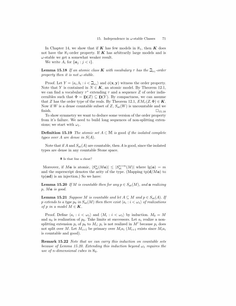
15. Independence in ω-stable Classes 71
In Chapter 14, we show that if K has few models in ℵ1, then K doesnot have the ℵ1-order property. If K has arbitrarily large models and isω-stable we get a somewhat weaker result.
We write Ai for {aj : j < i}.
Lemma 15.18 If an atomic class K with vocabulary τ has the iω1-orderproperty then it is not ω-stable.
Proof. Let Y = 〈ai, bi : i < iω1〉 and φ(x,y) witness the order property.Note that Y is contained in N ∈ K, an atomic model. By Theorem 12.1,we can find a vocabulary τ∗ extending τ and a sequence Z of order indis-cernibles such that Φ = D(Z) ⊆ D(Y ). By compactness, we can assumethat Z has the order type of the reals. By Theorem 12.1, EMτ (Z, Φ) ∈ K.Now if W is a dense countable subset of Z, Sat(W ) is uncountable and wefinish. ¤15.18
To show symmetry we want to deduce some version of the order propertyfrom it’s failure. We need to build long sequences of non-splitting exten-sions; we start with ω1.
Definition 15.19 The atomic set A ⊂M is good if the isolated completetypes over A are dense in S(A).
Note that if A and Sat(A) are countable, then A is good, since the isolatedtypes are dense in any countable Stone space.
Is that line a cheat?
Moreover, if Ma is atomic, |Snat(Ma)| ≤ |Sn+m
at (M)| where lg(a) = mand the superscript denotes the arity of the type. (Mapping tp(d/Ma) totp(ad) is an injection.) So we have:
Lemma 15.20 If M is countable then for any p ∈ Sat(M), and a realizingp, Ma is good.
Lemma 15.21 Suppose M is countable and let A ⊆ M and p ∈ Sat(A). Ifp extends to a type p0 in Sat(M) then there exist 〈ai : i < ω1〉 of realizationsof p in a model M ∈ K.
Proof. Define 〈ai : i < ω1〉 and 〈Mi : i < ω1〉 by induction. M0 = Mand a0 is realization of p0. Take limits at successors. Let ai realize a non-splitting extension pi of p0 to Mi; pi is not realized in M ′ because pi doesnot split over M . Let Mi+1 be primary over Miai (Mi+1 exists since Miai
is countable and good).
Remark 15.22 Note that we can carry this induction on countable setsbecause of Lemma 15.20. Extending this induction beyond ω1 requires theuse of n-dimensional cubes in ℵ0.

72 15. Independence in ω-stable Classes
Lemma 15.23 Suppose tp(ab/A) is based on some C ⊆ A. If a ^A
b and
b /A
a then some formula has the ℵ1-order property for K.
Proof. Suppose for contradiction that b /A
a. Then there is a formula
φ(x, z, y) and m ∈ A such that if b′^A
a and b′ ≡A b, then ¬φ(a,m, b′)
but φ(a,m, b). Now, let a = a0, b = b0; invoke Lemma 15.21 to choosefor i < ω1, bi+1 to realize the nonsplitting extension of tp(b/M) to AiBi
(guaranteed by Lemma 15.14 and then ai+1 to realize the nonsplittingextension of tp(a/M) to AiBi+1.
Case i < j: Since bj ^C
a0, by the choice of φ, we have ¬φ(a0,m, bj) and since
a0m ≡C aim, and bj ^C
Ai+1, ¬φ(ai,m, bj).
Case i ≥ j: We have φ(a0,m, b0) and a0 ≡Cmb0 ai so φ(ai,m, b0) holds. Furthertp(ai/ABj+1) does not split over A and bj ≡M b0 so φ(ai,m, bj)
Thus, φ(x,m, y) has the ω1-order property. ¤15.23
We need to write in the exact hypothesis when to order property situation isresolved.
Theorem 15.24 If a^A
b then b ^A
a.
The ‘ω-saturation’ eliminates for types over models the distinctions be-tween orthogonality and weak orthogonality that are important in the firstorder case.
Definition 15.25 Let p, q ∈ Sat(A) be stationary.
1. We say p is weakly orthogonal to q and write p ⊥w q if any realiza-tions of p and q respectively are independent over M .
2. We say p is orthogonal to q and write p ⊥ q if for any B ⊇ A withB ⊆ M ∈ K, p|B ⊥w q|B.
Note that p|B ⊥w q|B means p|B |= p|Ba, if a |= q|B.Since the nonsplitting independence relation satisfies transitivity, sym-
metry and monotonicity, we have by the same abstract argument as Corol-lary II.2.10 of [1].
Lemma 15.26 Suppose tp(a/A) and tp(b/A) are based in A. If ab ^A
B
then a^A
b iff a^B
b.
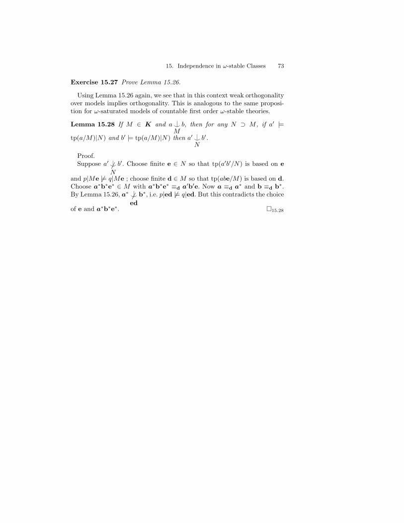
15. Independence in ω-stable Classes 73
Exercise 15.27 Prove Lemma 15.26.
Using Lemma 15.26 again, we see that in this context weak orthogonalityover models implies orthogonality. This is analogous to the same proposi-tion for ω-saturated models of countable first order ω-stable theories.
Lemma 15.28 If M ∈ K and a ^M
b, then for any N ⊃ M , if a′ |=tp(a/M)|N) and b′ |= tp(a/M)|N) then a′^
Nb′.
Proof.Suppose a′ /
N
b′. Choose finite e ∈ N so that tp(a′b′/N) is based on e
and p|Me 6|= q|Me ; choose finite d ∈ M so that tp(abe/M) is based on d.Choose a∗b∗e∗ ∈ M with a∗b∗e∗ ≡d a′b′e. Now a ≡d a∗ and b ≡d b∗.By Lemma 15.26, a∗ /
edb∗, i.e. p|ed 6|= q|ed. But this contradicts the choice
of e and a∗b∗e∗. ¤15.28

74 15. Independence in ω-stable Classes

This is page 75Printer: Opaque this
16Consequences of Excellence
Definition 16.1 The atomic aec K is excellent if
1. K is ω-stable;
2. Nonsplitting is symmetric.
3. For every n, K satisfies the (ℵ0, n)-existence property.
We need a little notation to define the (ℵ0, n)-existence property.
Notation 16.2 An independent (λ, n)-system is a family of models 〈Ms :s ⊂ n〉 such that:
1. Each Ms ∈ K has cardinality λ.
2. If s ⊆ t, Ms ≺K Mt.
3. For each s, As =⋃
t⊂s Mt is atomic.
4. For each s, Ms ^As
Bs where Bs =⋃
t 6⊂s Mt.
We follow [20] here; Shelah [31] uses (λ, n)-existence for a slightly differentproperty.
Definition 16.3 K satisfies (λ, n)-existence if there is a primary modelover
⋃t⊂n Mt for every independent (λ, n)-system.
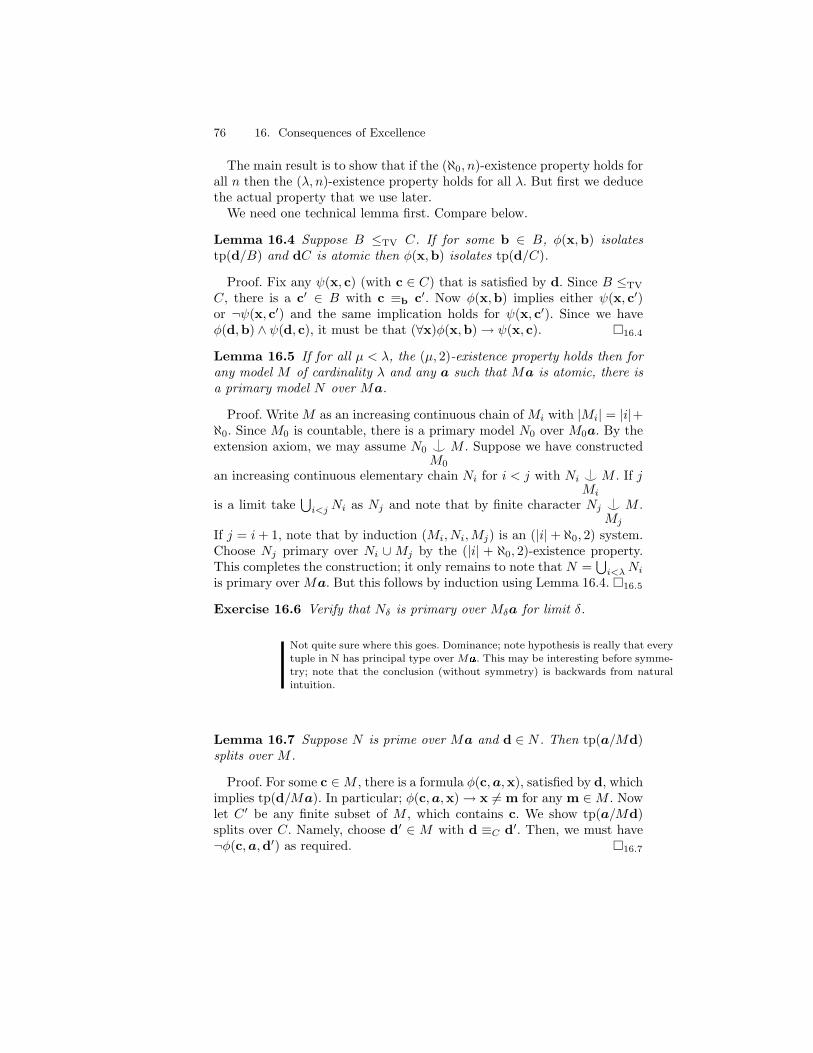
76 16. Consequences of Excellence
The main result is to show that if the (ℵ0, n)-existence property holds forall n then the (λ, n)-existence property holds for all λ. But first we deducethe actual property that we use later.
We need one technical lemma first. Compare below.
Lemma 16.4 Suppose B ≤TV C. If for some b ∈ B, φ(x,b) isolatestp(d/B) and dC is atomic then φ(x,b) isolates tp(d/C).
Proof. Fix any ψ(x, c) (with c ∈ C) that is satisfied by d. Since B ≤TV
C, there is a c′ ∈ B with c ≡b c′. Now φ(x,b) implies either ψ(x, c′)or ¬ψ(x, c′) and the same implication holds for ψ(x, c′). Since we haveφ(d,b) ∧ ψ(d, c), it must be that (∀x)φ(x,b) → ψ(x, c). ¤16.4
Lemma 16.5 If for all µ < λ, the (µ, 2)-existence property holds then forany model M of cardinality λ and any a such that Ma is atomic, there isa primary model N over Ma.
Proof. Write M as an increasing continuous chain of Mi with |Mi| = |i|+ℵ0. Since M0 is countable, there is a primary model N0 over M0a. By theextension axiom, we may assume N0 ^
M0
M . Suppose we have constructed
an increasing continuous elementary chain Ni for i < j with Ni ^Mi
M . If j
is a limit take⋃
i<j Ni as Nj and note that by finite character Nj ^Mj
M .
If j = i + 1, note that by induction (Mi, Ni,Mj) is an (|i|+ ℵ0, 2) system.Choose Nj primary over Ni ∪ Mj by the (|i| + ℵ0, 2)-existence property.This completes the construction; it only remains to note that N =
⋃i<λ Ni
is primary over Ma. But this follows by induction using Lemma 16.4. ¤16.5
Exercise 16.6 Verify that Nδ is primary over Mδa for limit δ.
Not quite sure where this goes. Dominance; note hypothesis is really that everytuple in N has principal type over Ma. This may be interesting before symme-try; note that the conclusion (without symmetry) is backwards from naturalintuition.
Lemma 16.7 Suppose N is prime over Ma and d ∈ N . Then tp(a/Md)splits over M .
Proof. For some c ∈ M , there is a formula φ(c, a,x), satisfied by d, whichimplies tp(d/Ma). In particular; φ(c, a,x) → x 6= m for any m ∈ M . Nowlet C ′ be any finite subset of M , which contains c. We show tp(a/Md)splits over C. Namely, choose d′ ∈ M with d ≡C d′. Then, we must have¬φ(c, a,d′) as required. ¤16.7

This is page 77Printer: Opaque this
17Quasiminimal Sets in Excellent Classes
In this chapter we introduce a notion of *-excellence which is intermedi-ate in strength between Shelah’s and Zilber’s notion. We will constructquasiminimal formulas in a *-excellent class and begin the definition of anindependence notion analogous to nonforking in first order logic.
This chapter is indirectly based on [28, 30, 31], where most of the resultswere originally proved. But our exposition owes a great deal to [20, 19, 17,10].
Recall that a model M is atomic if every finite sequence in M realizes aprincipal type over the empty set. Thus if T is ℵ0-categorical every modelof T is atomic.
Following Lessmann, we give another meaning to ‘excellent’:
Definition 17.1 The atomic class K is *-excellent if
1. K is ω-stable.
2. K satisfies the amalgamation property
3. Let p be a complete type over a model M ∈ K such that p ¹ C isrealized in M for each finite C ⊂ M , then there is a model N ∈ Kwith N primary over Ma such that p is realized by a in N .
Our goals are:
1. Show in ZFC that *-excellent classes satisfy Morley’s theorem.
2. Show assuming the weak continuum hypothesis that if an atomic classK is categorical up to ℵω, then it is ∗-excellent.

78 17. Quasiminimal Sets in Excellent Classes
We have verified in Chapter ?? that excellence implies Conditions 2(STILL TO DO) and 3. We now show that this implies that Galois-typesare syntactic types in this context and that K has arbitrarily large models.
delete?? Lessmann ([19] also assumes that K has arbitrarily large models butas we see below that is a actually a consequence of ∗-excellence as describedhere. That hypothesis yields ω-stability easily by Lecture 5, but ω-stability canbe gotten more cheaply (or at least at a different price) as we will see below.
Note that types over sets make syntactic sense as in first order logic, butwe have to be careful about whether they are realized. By 3) of Defini-tion 17.1, p ∈ Sat(M) if and only if p ¹ C is realized in M for each finiteC ⊂ M .
think about next two.
Exercise 17.2 If M ≺ N ∈ K, where K is *-excellent and p ∈ Sat(M)then p extends to q ∈ Sat(N).
Lemma 17.3 If K is *-excellent then Galois types over a model M arethe same as syntactic types in Sat(M).
Proof. Equality of Galois types is always finer than equality of syntactictypes. But if a, b realize the same p ∈ Sat(M), by 2) of Definition 17.1, wecan map Ma into any model containing Mb and take a to b so the Galoistypes are the same. ¤17.3
Note however, we have more resources here than in a general AEC. Thetypes in Sat(A) for A atomic play an important role; in general there is nonotion of types over all subsets of models of K.
Lemma 17.4 Let A ⊆ M and p ∈ Sat(A). TFAE:
1. There is an N with M ≺ N and c ∈ N −M realizing p; i.e. p extendsto a type in Sat(M).
2. For all M ′ with M ≺ M ′ there is an N ′, M ′ ≺ N ′ and some d ∈N ′ −M ′ realizing p.
Proof: 2) implies 1) is immediate. For the converse, assume 1) holds.Without loss of generality, by amalgamation, M ′ contains N . Let q =tp(c/M). By Theorem 15.8, there is a nonsplitting extension q of q toSat(M ′). By Assumption 17.1 3) q is realized in N ′ ∈ K. Moreover, it isnot realized in M ′ because q does not split over M . ¤17.4
For countable M ′, we will see below how to get M ′ via the omitting typestheorem. But the existence of N ′ for uncountable cardinalities requires theuse of n-dimensional cubes in ℵ0.

17. Quasiminimal Sets in Excellent Classes 79
Definition 17.5 The type p over A ⊆ M ∈ K is big if for any M ′ ⊇ Athere exists an N ′ with M ′ ≺K N ′ and with a realization of p in N ′−M ′.
By iteratively applying Lemma 17.4, we can show:
Corollary 17.6 Let A ⊆ M and p ∈ Sat(A). If there is an N with M ≺ Nand c ∈ N −M realizing p then
1. p is big and
2. K has arbitrarily large models.
Thus every nonalgebraic type over a model and every type with uncount-ably many realizations (check the hypothesis via Lowenheim-Skolem) is big.But if we consider K to contain only one model: two copies of (Z, S), wesee a type over a finite set can have infinitely many realizations withoutbeing big.
With this technology we can prove a nice result. Let’s update our notionof saturation for this context.
Definition 17.7 1. The model M ∈ K is λ-full over A ⊂ M if forevery C ⊂ M with |C| < λ, if p is based on A then p|AC is realizedin M .
2. M is λ full if for every A ⊂ M with |A| < λ and every p ∈ Sat(A)that is based in A, is realized in M .
We use clause 1) when constructing for example countable models Mwhich are full over a countable set A.
We would like to have the hypothesis be ω-stable atomic class with amalgama-tion. But we don’t know in general that ‘every p based on A can be extendedto p ∈ Sat(MA) for MA with A ⊂ MA ⊂ M ’.
Lemma 17.8 Let K be a *-excellent class.Suppose |M | = λ > ℵ0. Then M is Galois-saturated if and only if M is
λ-full.
Proof. Since ω-stability implies that if p ∈ Sat(N) then p is based onN , a full model is Galois-saturated. But since every p based on A can beextended to p ∈ Sat(MA) for MA with A ⊂ MA ⊂ M and |A| = |MA|,every Galois-saturated model is full. ¤17.8
Lemma 17.9 Let K be an ω-stable atomic class. If Mi : i < δ for δ ≤ λare λ-full with λ uncountable then M =
⋃i<δ Mi is also λ-full.
Proof. This is immediate if δ < cf(λ). Let A ⊂ M with |A| < λ andsuppose p ∈ Sat(A) is based on d ∈ A. Let r ∈ Sat(M) be the unique

80 17. Quasiminimal Sets in Excellent Classes
nonsplitting extension of p to Sat(M). Without loss of generality d ∈ M0.Let ai for i < δ enumerate all finite tuples from A. For each ai, choosea finite subset Xi of M0 such that tp(ai/M0) is based on Xi, Using theλ-fullness of M0, construct E ⊂ M0 such that E = 〈ei : i < δ + 1〉 andNi for i < λ such that: d ∈ N0, for i < δ, Xi ∈ Ni |Ni| = |Ei| + LS(K),M0Ei ⊂ Ni, tp(ei/Ni) = r|Ni. Let note |Nδ| < λ. Then A ^
NM0. Let
e = eδ. By symmetry e ^N
A and by the choice of N , e ^d
N . By transitivity
e realizes r|A = p and we finish.
Theorem 17.10 Let K be a *-excellent class. Then K has λ-full modelsof cardinality λ for all λ.
Proof. Note that by the proof of Lemma 11.15 (Note only stability wasused to get the saturated model.) we have a Galois-saturated model ofcardinality λ for every uncountable regular λ. Now for singular λ take asequence of λi saturated models for λi tending to λ and apply Lemma 17.9to get a model M which is λi-saturated for each λi. But then it is λ-saturated since the λi sup to λ. ¤17.10
Definition 17.11 The type p ∈ Sat(A) is quasiminimal if p is big and forany M containing A, p has a unique extension to a type over M which isnot realized in M .
Note that whether q(x, a) is big or quasiminimal is a property of tp(a/∅).Since every model is ω-saturated the minimal vrs strongly minimal diffi-culty does not arise.
Now almost as one constructs a minimal set in the first order context,we find a quasiminimal type; for details see [19]
Lemma 17.12 Let K be excellent. For any M ∈ K, there is a c ∈ M anda formula φ(x, c) which is quasiminimal.
Proof. It suffices to show the countable model has a quasiminimal formulaφ(x, c) (since quasiminimality of depends on the type of c over the emptyset). As in the first order case, construct a tree of formulas which arecontradictory at each stage and are big. But as in the proof of Lemma 15.7make sure the parameters in each infinite path exhaust M . Then, if we canconstruct the tree ω-stability is contradicted as in Lemma 15.7. So there isa quasiminimal formula. ¤17.12
Definition 17.13 Let c ∈ M ∈ K and suppose φ(x, c) generates a quasi-minimal type over M . For any elementary extension N of M define cl onthe set of realizations of φ(x, c) in N by a ∈ cl(A) if tp(a/Ac) is not big.
Equivalently, we could say a ∈ cl(A) if every realization of tp(a/Ac) iscontained in each M ′ ∈ K which contains Ac.

17. Quasiminimal Sets in Excellent Classes 81
Lemma 17.14 Let c ∈ M ∈ K and suppose φ(x, c) generates a quasi-minimal type over M . If the elementary extension N of M is full with|N | > |M |, then cl defines a pregeometry on the realizations of φ(x, c) inN .
Proof. Clearly for any a and A, a ∈ A implies a ∈ cl(A). To see that clhas finite character note that if tp(a/Ac) is not big, then it differs from theunique big type over Ac and this is witnessed by a formula so a is in theclosure of the parameters of that formula.
For idempotence, suppose a ∈ cl(B) and B ⊆ cl(A). Use the commentafter Definition 17.13 Every M ∈ K which contains A contains B andevery M ∈ K which contains B contains a; the result follows.
It is only to verify exchange that we need the fullness of N . Supposea, b |= φ(x, c), each realizes a big type over A ⊆ φ(N) and r = tp(b/Aac) isbig. Since r = tp(a/Ac) is big and N is full we can choose λ realizations ai
of r in N . Let M ′ ≺ N contain the ai and let b′ realize the unique big typeover M ′ containing φ(x, c). Since tp(b/Aac) is big, the uniqueness yieldsall pairs (ai, b
′) realize the same type p(x, y) ∈ S(Ac) as (a, b). But thenthe ai are uncountably many realization of tp(a/Abc) so this type is big aswell; this yields exchange by contraposition. ¤17.14
So the dimension of the quasiminimal set is well-defined. To concludecategoricity, we must show that dimension determines the isomorphismtype of the model; this is the topic of the next chapter.

82 17. Quasiminimal Sets in Excellent Classes

This is page 83Printer: Opaque this
18Two Cardinal Models and CategoricityTransfer
We work in a *-excellent atomic class K. That is, K is the class of atomicmodels of a first order theory T , which was obtained from a complete sen-tence in Lω1,ω by adding predicates for all formulas in a countable fragmentL∗ of Lω1,ω. The vocabulary for K is τ .
Definition 18.1 The type p(x) ∈ Sat(M) is definable over the finite setc if for each formula φ(x) there is a formula (dpx)φ(x,y)[y, c] with freevariable y such that (dpx)φ(x,y)[m, c] holds for exactly those m ∈ M suchthat φ(x,m) ∈ p. This is a defining schema for p.
The following lemma is taken without proof (or even mention) in theproof of Lemma 4.2 of [28]. In the proof we expand the language but in away that does no harm.
Lemma 18.2 There is an atomic class K1 in a vocabulary τ1, whose mod-els are in 1-1 correspondence with those of K such that: for each τ1-formulaφ(x,y) and countable ordinal α, there is a τ1-formula Pφ,α(y) such that inany model M in K1, Pφ,α(m) holds if and only if RM (φ(x,m)) ≥ α.
Proof. Define a sequence of classes and vocabularies τ i, Ki by adjoiningpredicates in τ i+1 which define rank for τ i-formulas. Note that reduct is a1-1 map from τω structures to τ -structures. Then τω, Kω are the requiredτ1, K1. ¤18.2
Henceforth, we assume K satisfies the conclusion of Lemma 18.2.
Lemma 18.3 Let K be ω-stable. Every type over a model is definable.

84 18. Two Cardinal Models and Categoricity Transfer
Proof. Now let N be an atomic model of T and let p ∈ Sat(N); chooseφ(x, c) so that R(p) = R(φ(x, c)) = α. Now for any ψ(x,d), ψ(x,d) ∈ pif and only if R(φ(x, c) ∧ ψ(x,d)) = α. And, the collection of such m isdefined by Pφ(x,c)∧ψ(x,y),α(y, c). ¤18.3
Note that if p doesn’t split over C with C ⊂ M ≺ N and p ∈ Sat(M) isa nonsplitting extension of p, p is defined by the same schema as p.
We abuse standard notation from e.g. [18] in our context. Note that wehave restrict our attention to big formulas. This will give us two cardinaltransfer theorems that read exactly as those for first order but actuallyhave different content because the first order versions refer arbitrary infinitedefinable sets.
Definition 18.4 1. A triple (M, N, φ) where M ≺ N ∈ K withM 6= N , φ is defined over M , φ big, and φ(M) = φ(N) is calleda Vaughtian triple.
2. We say K admits (κ, λ), witnessed by φ, if there is a model N ∈ Kwith |N | = κ and |φ(N)| = λ and φ is big.
Of course, it is easy in this context to have definable sets which arecountable in all models. But we’ll show that this is really the only sensein which excellent classes differ from stable theories as far as two cardinaltheorems are concerned.
The overall structure of the proof of the next result is based on Propo-sition 2.21 of [20]; but in the crucial type omitting step we expand theargument of Theorem IX.5.13 in [1] rather than introducing nonorthogo-nality arguments at this stage.
Lemma 18.5 Suppose K is *-excellent.
1. If K admits (κ, λ) for some κ > λ then K has a Vaughtian triple.
2. If K has a Vaughtian triple, for any (κ′, λ′) with κ′ > λ′, K admits(κ′, λ′).
Proof. Suppose N ∈ K with |N | = κ and |φ(N)| = λ. For notationalsimplicity we add the parameters of φ to the language. By Lowenheim-Skolem, we can embed φ(N) in a proper elementary submodel M and get aVaughtian triple. We may assume that M and N are countable. To see this,build within the given M,N countable increasing sequences of countablemodels Mi, Ni, fixing one element b ∈ N −M to be in N0 and choosingMi ≺ M , Ni ≺ N , Mi ≺ Ni and φ(Ni) ⊂ φ(Mi+1). Then Mω, Nω are asrequired.
Now for any κ′, we will construct a (κ′, ω) model. Say b ∈ N −M andlet q = tp(b/M). Now construct Ni for i < κ′ so that Ni+1 is primaryover the Nibi where bi realizes the non-splitting extension of q to Sat(Ni).Fix finite C contained in M so that q does not split over C. We prove by
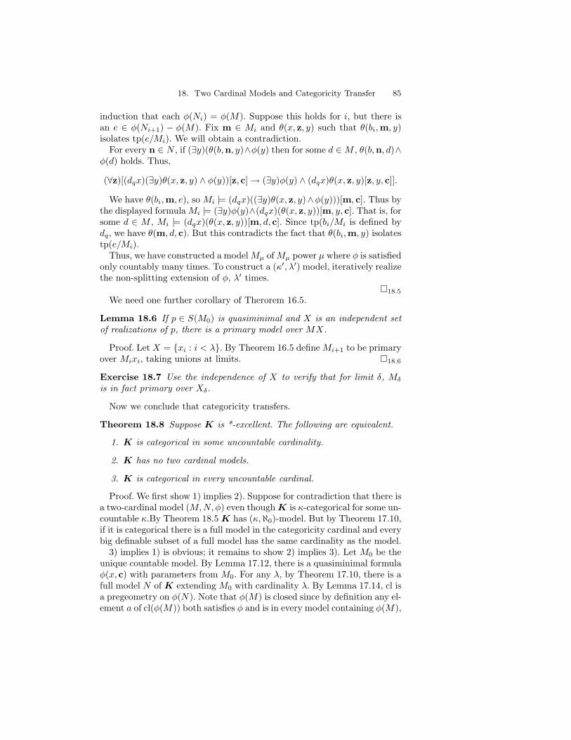
18. Two Cardinal Models and Categoricity Transfer 85
induction that each φ(Ni) = φ(M). Suppose this holds for i, but there isan e ∈ φ(Ni+1) − φ(M). Fix m ∈ Mi and θ(x, z, y) such that θ(bi,m, y)isolates tp(e/Mi). We will obtain a contradiction.
For every n ∈ N , if (∃y)(θ(b,n, y)∧φ(y) then for some d ∈ M , θ(b,n, d)∧φ(d) holds. Thus,
(∀z)[(dqx)(∃y)θ(x, z, y) ∧ φ(y))[z, c] → (∃y)φ(y) ∧ (dqx)θ(x, z, y)[z, y, c]].
We have θ(bi,m, e), so Mi |= (dqx)((∃y)θ(x, z, y)∧φ(y)))[m, c]. Thus bythe displayed formula Mi |= (∃y)φ(y)∧(dqx)(θ(x, z, y))[m, y, c]. That is, forsome d ∈ M , Mi |= (dqx)(θ(x, z, y))[m, d, c]. Since tp(bi/Mi is defined bydq, we have θ(m, d, c). But this contradicts the fact that θ(bi,m, y) isolatestp(e/Mi).
Thus, we have constructed a model Mµ of Mµ power µ where φ is satisfiedonly countably many times. To construct a (κ′, λ′) model, iteratively realizethe non-splitting extension of φ, λ′ times.
¤18.5
We need one further corollary of Therorem 16.5.
Lemma 18.6 If p ∈ S(M0) is quasiminimal and X is an independent setof realizations of p, there is a primary model over MX.
Proof. Let X = {xi : i < λ}. By Theorem 16.5 define Mi+1 to be primaryover Mixi, taking unions at limits. ¤18.6
Exercise 18.7 Use the independence of X to verify that for limit δ, Mδ
is in fact primary over Xδ.
Now we conclude that categoricity transfers.
Theorem 18.8 Suppose K is *-excellent. The following are equivalent.
1. K is categorical in some uncountable cardinality.
2. K has no two cardinal models.
3. K is categorical in every uncountable cardinal.
Proof. We first show 1) implies 2). Suppose for contradiction that there isa two-cardinal model (M, N, φ) even though K is κ-categorical for some un-countable κ.By Theorem 18.5 K has (κ,ℵ0)-model. But by Theorem 17.10,if it is categorical there is a full model in the categoricity cardinal and everybig definable subset of a full model has the same cardinality as the model.
3) implies 1) is obvious; it remains to show 2) implies 3). Let M0 be theunique countable model. By Lemma 17.12, there is a quasiminimal formulaφ(x, c) with parameters from M0. For any λ, by Theorem 17.10, there is afull model N of K extending M0 with cardinality λ. By Lemma 17.14, cl isa pregeometry on φ(N). Note that φ(M) is closed since by definition any el-ement a of cl(φ(M)) both satisfies φ and is in every model containing φ(M),

86 18. Two Cardinal Models and Categoricity Transfer
including M . Thus we can choose a basis X for φ(M). By Theorem 18.6,there is a prime model M|X| over MX. But X ⊂ φ(M|X|) ⊂ φ(M) soφ(M|X|) = φ(M); whence since we assume there are no two cardinal mod-els, M|X| = M and M is prime and minimal over MX.
Now we show categoricity in any uncountable cardinality. If M , N aremodels of power λ, they are each prime and minimal over X, a basis forφ(M) and Y , a basis for φ(N), respectively. Now any bijection between Xand Y is elementary by the moreover clause in Lemma 17.14. It extends toa map from M into N by primeness and it must be onto; otherwise thereis a two cardinal model. ¤18.8
This is page 87Printer: Opaque this
19Demystifying Non-excellence
In this chapter we expound the Hart-Shelah example of a sentence ψ inLω1,ω which is categorical in ℵ0,ℵ1 but not in 2ℵ1 . More generally for eachk the construction provides a sentence which is categorical up to ℵk but notcategorical everywhere. We outline the general construction but specializeto k = 2 for many specific arguments.
This example is a descendent of the example in [3] of an ℵ1-categoricaltheory which is not almost strongly minimal. That is, the universe is notin the algebraic closure of a strongly minimal set. Here is a simple way todescribe such a model. Let G be a strongly minimal group and let π mapX onto G. Add to the language a binary function t for the fixed-point freeaction of G on π−1(g) for each g ∈ G. This guarantees that each fiber hasthe same cardinality as G and π guarantees the number of fibers is thesame as |G|. Since there is no interaction among the fibers, categoricity inall uncountable powers is easy to check.
19.1 The basic structure
Notation 19.1 The formal language for this example contains unary pred-icates W,Z2, I,K, Ga, G∗,Ha, H∗; binary functions eG taking G×K to Z2
and eH taking H ×K to Z2; function πG mapping G∗ to W ×K, functionπH mapping H∗ to K, a 5-ary relation t on W ×K × Ga × G∗ × G∗), a4-ary relation symbol h, K ×Ga ×H∗ ×H∗), and ternary relations q` on

88 19. Demystifying Non-excellence
for ` < ω on G∗ ×G∗ ×H∗. Certain other projection functions are in thelanguage but not expressly described.
We will construct a structure M(I) from any infinite set I. The structurewill be a disjoint union of sets I, K, Z2, G
a,Ha, G∗ and H∗. All except G∗
and H∗ will be completely determined by I. For standard structures G∗
and H∗ will also be completely determined. Let K = [I]k be the set of kelement subsets of I and let G be the direct sum of K copies of Z2 so G andK have the same cardinality. We are going to put a structure on K × G.(A priori, we might as well have indexed by I! The connection with K willonly appear with the introduction of the Q` at the end of the construction.)
The basic object in the construction is a family of copies of the groupG, indexed by a set W ×K. W will be a copy of ω, which is required toprovide some coding in the non-categoricity proof; we point this out atthe appropriate time. We add constants c` for the elements of W and thesentence ψ saying they exhaust W . The basic object should be categoricalin all powers. This is achieved in two steps. We include K, Ga (naming G)and Z2 as sorts of the structure with the evaluation function: for γ ∈ G andk ∈ K, eG(γ, k) = γ(k) ∈ Z2. So in Lω1,ω we can say that the predicateGa denotes exactly the set of elements with finite support of KZ2. Now,we introduce a set G∗. We say a model is G-standard if G∗ is W ×K ×Gbut we don’t have all the projection functions which would allow us to saythat. Rather we have only the projection function πG from G∗ onto W×K.We write v ∈ G`,u when πG(v) = (`, u) and say v is in the (G)-stalk over`, u. Thus, W × K indexes a partition of G∗. The relation t(`, u, v, w, x)is the graph of the action (by addition) of Ga on each member G`,u ofthe partition indexed by W × K. That is t(`, u, v, w, x) holds where w =(`, u, w′), x = (`, u, x′), v ∈ G and v + w′ = x′. So each class is an (affine)copy of G.
This much of the structure is clearly categorical (and homogeneous). Sowe must work harder.
We consider a new group H, the direct sum of ω copies of Z2 (againexplicitly represented as a subset Ha of W Z2, with a sort for W and theevaluation function, eH). Again we add a set H∗ and a function πH takingH∗ to K. When H∗ is K ×H, we say the model is H-standard. As beforeπH(x) = u holds if x has the form (u, x′). Finally h(u, v, w, x) is the graphof the action (by addition) of Ha on each member Hu of the partition ofH∗ indexed by K.
This structure is still categorical. To see this, suppose two such modelshave been built on I and I ′ of the same cardinality. Take any bijectionbetween I and I ′. To extend the map to G∗ and H∗ fix one element in eachpartition class in each model. The natural correspondence (linking thoseselected in corresponding classes) extends to an isomorphism.
The key step is the definition of a family of relations Q` that witness thefailure of k-dimensional amalgamation. For concreteness we fix k = 2. The

19.2 k = 2, ℵ1-categoricity 89
structure is imposed by a family of 3-ary relations Q` on G∗ × G∗ × H∗,which have a local character. Q` only holds of elements with first coordinate`. Moreover, Q`((`, u1, x1), (`, u2, x2), (u3, x3)) implies that u1, u2, u3 arethe three two element subsets of a 3 element subset of I. We call u1, u2, u3
a compatible triple. (Suitable projections are in the language to expressthis.) Finally, Q`((`, u1, x1), (`, u2, x2), (u3, x3)) holds just if
x1(u3) + x2(u3) = x3(`).
This completes the description of the example.
19.2 k = 2, ℵ1-categoricity
We now show that with k = 2 the structure is ℵ1-categorical. We chooseglobal sections for the maps πG and πH .
Definition 19.2 Fix a model M . A solution for M is a selector f thatchooses one element of the fiber in G∗ above each element of W ×K andone element of the fiber in H∗ above each element of K. Formally, f isa pair of functions (f0, f1), where f0 : W (M) × K(M) → G∗(M) andf1 : K(M) → H∗(M) such that πGf0 and πHf1 are the identity and foreach ` and compatible triple u1, u2, u3,:
Q`([(`, u1), f0(`, u1)], [(`, u2), f0(`, u2)], (u3, f1(u3))).
Lemma 19.3 If M and N have the same cardinality and have solutionsfM and fN then M ∼= N .
Proof. Without loss of generality, M = M(I), N = M(I ′). Let α be anarbitrary bijection between I and I ′. Extend naturally to a map from K(M)to K(N) and from Ga(M),Ha(M) to Ga(N),Ha(N); let α(fM (`, u)) befN (`, α(u)). If x ∈ G∗(M), and M |= πG(x) = (`, u), there is a uniquea ∈ Ga(M) such that
M |= t(c`, u, a, fM (`, u), x).
Let α(x) be the unique y ∈ N such that
N |= t(c`, α(u), α(a), fN (`, u), y).
Do a similar construction for H∗ and observe that each Q` is preserved.¤19.3
Slightly more generally, we describe selectors over subsets of I(M) ratherthan all of I(M).

90 19. Demystifying Non-excellence
Definition 19.4 There is a solution for the subset A of I(M) if for each2-set u from [A]2 and each ` there are f0(`, u) ∈ G`,u and f1(u) ∈ Hu suchthat if u1, u2, u3 are a compatible triple from A2, for every `,
Q`([(`, u1), f0(`, u1)], [(`, u2), f0(`, u2)], (u3, f1(u3))).
Fact 19.5 If |M | ≤ ℵ1, M has a solution.
Proof. Note first that it suffices to show that if there is a solutionf = (f0, f1) over a countable set A ⊂ I(M) then for any b ∈ I(M) itcan be extended to a solution f ′ = (f ′0, f
′1) over A ∪ {b}. To show the
extension property, enumerate A as ai for i < ω. For each i, choose ar-bitrarily f ′1(ai, b) ∈ Hai,b. Then prove by induction on n that f0 can befurther extended to a solution f ′0 over all tuples (`, (ai, b)) for `, i ≤ n. Atthe induction step, we must define f ′0(`, (an+1, b)) compatibly with our pre-vious choices of the f ′0(`, (an+1, ai)) and f ′1((ai, b)) for i ≤ n. This abilityis guaranteed by the following fact which holds in the original structureas the conditions fix only a finite number of values of the element to bechosen. ¤19.5
Fact 19.6 If ` ∈ W , a1, . . . an+1, b are in I, xj ∈ Gc`,(an,aj) for 1 ≤ j ≤ n,and for each 1 ≤ j ≤ n, yj ∈ Hb,aj then
(∃x)∧
1≤j≤n
πG(x) = (`, (aj , b)) ∧Q`(x, xj , yj).
But we are stymied at ℵ2 since adding any new point to a set of size ℵ1
gives us ℵ1 conditions to meet.
19.3 k = 3, ℵ2-categoricity
The argument above seems to depend only on ℵ0-homogeneity and doesn’tillustrate how the categoricty is carried to higher cardinalities by increasingk. But the idea becomes clearer if we take k equal to 3.
Here is a soft argument that moves from a configuration of countablemodels to categoricity in higher cardinals. We have already seen that iffor A ⊆ B, both with cardinality ℵn, A-solutions extend to B-solutionsthen there is a solution for sets of cardinality ℵn+1. So to get a solution ofcardinality ℵ2 we need to have extension at ℵ1. Again, it suffices to extenda set of cardinality ℵ1 by one point. Writing the set as union of countablesets, it suffices to be able to amalgamate the solutions of two one pointextensions of a countable set.
We show that 3-dimensional amalgamation holds in ℵ0, when k = 3.
Lemma 19.7 Let k = 3. Let A be a countable subset of I, b0, b1 ∈ I−A. Iff = (f0, f1) and g = (g0, g1) are solutions over A0 = A∪{b0}, A1 = A∪{b1}

19.4 Failure of Categoricity in 2ℵ1 91
respectively, which agree on A, there is a solution h over A01 = A∪{b0, b1}which extends both g and f .
Proof. With k = 3, the object of interest is a compatible four tupleu0, u1, u2, u3, the four 3-element subsets of b0, b1, b2, b3. For each ` thereare two of the four arguments of Q` that have not been defined by g or f .Show the analog to Fact 2. ¤19.7
It is instructive to try to show amalgamation for countable sets withk = 2; the assymetry between the selectors for H∗ and G∗ and the diago-nalization combine to frustrate such an attempt.
For larger n, one shows n-dimensional amalgamation on ℵ0 descendsstep by step to 2-dimensional amalgamation on ℵn−2, and thus extensionon ℵn−1 and categoricity in ℵn.
19.4 Failure of Categoricity in 2ℵ1
In general φ is not 2ℵk−1 -categorical; so for the k = 2 case, we will have φis ℵ0 and ℵ1 categorical but not 2ℵ1 -categorical.
Fix the least λ with λℵ1 < 2λ. Clearly, λ is between ℵ1 and 2ℵ1 . Wewill show φ has 2λ models of power λ. It is easy to see that if K is notcategorical in some κ; it not categorical in any larger κ′. There is a modelof power κ′ which has solution, so κ′-categoricity implies the unique modelhas a solution; but then so do all its submodels, which include all modelsof power κ. Thus, κ′-categoricity implies κ-categoricity and in particular ifwe show the failure of λ-categoricity we have the failure in 2ℵ1 .
Let H1 denote ⊗ωZ2.
Notation 19.8 For any map h from K to H1/H we define a model Mh(I).The structure is identical to the standard structures defined above with oneexception: the fibers π−1
H (x) are not copies of H but are the cosets h(u).That is, we have a structure which is G-standard but not H-standard.
As structures under the ‘action language’, h(u) and H are isomorphic.But in the concrete representation the elements of H have finite supportwhile the elements of h(u) have infinite support. Our goal is to recognizethis and more precisely to recognize h(u). The Lω1,ω sentence ψ forces Ga
and Ha to be elements of finite support, but we can’t force this for thefibers in G∗ (H∗) because the projection (in the standard model) from G∗
to G (H∗ to H) is not in the language.To show the failure of categoricity we will constructed a specific family
of models, the MA. Each model is G-standard but some stalks in H∗(MA)do not have finite support. With d as an oracle we will recover h from Mh.

92 19. Demystifying Non-excellence
Definition 19.9 1. Fix a selector for G∗ by defining a function d:d((`, u)) = (`, u, e) where e is the identically 0 element of G; we calld the identity selector.
2. Let u3 = {y, z}, u1 = {x, y}, u2 = {x, z} be in K. Define the mapηd
M (u3) from K into H1/H by ηdM (u3){`} = 0 if
M |= Q`([`, u1, d(`, u1)], [`, u2, d(`, u2)], [u3, c]).
where c is an arbitrary element of Hu3 . The choice of c will varyηd
M (u3) within a coset of H1/H.
3. We may write ηM (u3) when d is the identity selector.
So if we have the identity selector d, we can compute the coset ηM (u) atevery u and the value of ηM (u) does not depend on which third point fromI we choose to construct a compatible triple.
But this procedure names |M | points; we fixed d. We will see how toproceed naming only ℵ1-constants. Since λℵ1 < 2λ this will cause no harm;we will guarantee that in the expanded language there are 2λ models ofcardinality λ.
We choose the set I in a very particular way and then the function h.Let I be X ∪ ℵ1 × ℵ1 ∪ A where |X| = ℵ0 and A is a set of λ functionsa : ℵ1 → H/H1.
We define models (Mh(I), d) but I depends on the choice of A and wewill define the h uniformly for all A so we write: (MA, d). The crucialpoint is the choice of the H-stalks over those members of K that have theform (a, 〈α, β〉). For a ∈ A and 〈α, β〉 ∈ ℵ1 × ℵ1, the map h is definedby h(a, 〈α, β〉) = a(α). That is, the fiber H(a,〈α,β〉) is the coset a(α). Toavoid interference, we set h(u) = H for all other u. Again, define d byd((`, u)) = (`, u, e) where e is the identically 0 element of G.
Computing ηdMA
, yields ηdMA
(a, 〈α, β〉) is a(α) since the coset H(a,〈α,β〉)is a(α). Now suppose d is replaced by a d′ which agrees with d on X ×(ℵ1×ℵ1) but may disagree elsewhere. (I.e. expand the language by namingℵ1 constants.)
The invariant ηd′MA
(〈α, β〉, a)) is a function h ∈ H1 = 2ω. We complete(〈α, β〉, a) to a triple by choosing an element n from X; h is computed inthe model by h(`) = 0 if and only if
M |= Q`([`, (n, 〈α, β〉), d′(`, (n, 〈α, β〉)], [`, (n, a), d′(`, (n, a))], [(a, 〈α, β〉), c])
where c is an arbitrary element of the H-stalk over (〈α, β〉, a). Since d and d′
are equal on stalks above elements of the form (n, 〈α, β〉), the value of h onthe (a, 〈α, β〉)-stalks is determined by d′(`, (n, a)){(〈α, β〉, a)}. The relevantvalues are at the (〈α, β〉, a) where d′(`, (n, a)){(〈α, β〉, a)} 6= 0. There areof course only countably many of these for any (n, a) (finitely many for

19.5 Failure of tameness 93
any (`, (n, a)). As long as there is no ` with d′(`, (n, a)){a, 〈α, β〉} 6= 0,ηz
MA(〈α, β〉, a) is the same function whether calculated with z as d or d′.
Since this happens for cocountably many β, we finish. That is h ∈ H1/H
is in the range of a just if for ℵ1 elements i of I, ηd′MA
(i, a) = h. A is a setof λ functions from ℵ1 into H1/H. The range of an element of a is a subsetof 2ℵ0 . So there are 22ℵ0 possible sets of ranges and 22ℵ0 ≥ 2λ so there are2λ nonisomorphic models MA with cardinality λ.
This completes the argument for k = 2; we leave the nontrivial extension[11] of the coding to obtain the result for larger k to the reader.
19.5 Failure of tameness
We continue the notation of the non-categoricity argument in Section 19.4and note that there is a syntactic type p over a model of cardinality λ whichsplits into several Galois types. Since over countable models Galois typesand syntactic types are the same this implies that p is not determined byits restrictions to countable submodels. Thus mod(φ) is not (ℵ1,ℵ0)-tame.Let A0 ⊂ A1 be sets of functions of cardinality λ. By ℵ1-categoricity M issaturated. Let M = MA0 . By ℵ1-categoricity M is saturated so it suffices tofind a syntactic type over M which splits into several Galois types. Supposea, a′ ∈ A1−A0 and suppose the range of a and the range of a′ are different.In particular, assume there is h ∈ H1/H which is in the range of a butnot the range of a′. Then there can be no map fixing a model containingX ∪ ℵ1 × ℵ1, in particular M , which maps a to a′. Because for any d′
which is the identity selector when restricted to M , for ℵ1 elements i of I,ηd′
MA(i, a) = h but ηd′
MA(i, a′) = h for only countably many i in I. But a
and a′ realize the same syntactic type over M , since we can map one theother by while fixing any finite subset of M .
94 19. Demystifying Non-excellence

This is page 95Printer: Opaque this
References
[1] J.T. Baldwin. Fundamentals of Stability Theory. Springer-Verlag,1988.
[2] J.T. Baldwin and K. Holland. Constructing ω-stable structures: Rank2 fields. Journal of Symbolic Logic, 65:371–391, 2000.
[3] J.T. Baldwin and A.H. Lachlan. On strongly minimal sets. Journalof Symbolic Logic, 36:79–96, 1971.
[4] S. Buechler and O. Lessmann. Simple homogeneous models. Journalof the American Mathematical Society, 16:91–121, 2003.
[5] Steven Buechler. Essential Stability Theory. Springer-Verlag, 1991.
[6] C.C. Chang and H.J Keisler. Model theory. North-Holland, 1973.
[7] R. Grossberg. A course in model theory. preprint.
[8] R. Grossberg and M. Van Dieren. Galois stability for tame abstractelementary classes. preprint.
[9] Rami Grossberg. Classification theory for non-elementary classes. InYi Zhang, editor, Logic and Algebra, pages 165–204. AMS, 2002. Con-temporary Mathematics 302.
[10] Rami Grossberg and Bradd Hart. The classification theory of excellentclasses. Journal of Symbolic Logic, 54:1359–1381, 1989).
96 References
[11] Bradd Hart and Saharon Shelah. Categoricity over P for first order t orcategoricity for φ ∈ lω1ω can stop at ℵk while holding for ℵ0, · · · ,ℵk−1.Israel Journal of Mathematics, 70:219–235, 1990.
[12] W. Hodges. Model Theory. Cambridge University Press, 1993.
[13] B. Jonsson. Universal relational systems. Mathematica Scandinavica,4:193–208, 1956.
[14] B. Jonsson. Homogeneous universal relational systems. MathematicaScandinavica, 8:137–142, 1960.
[15] H.J. Keisler. Logic with quantifier ”there exists uncountably many”.Annals of Math. Logic, 1:1–93, 1970.
[16] H.J Keisler. Model theory for Infinitary Logic. North-Holland, 1971.
[17] A. Kolesnikov. Dependence relations in nonelementary classes.preprint.
[18] D. Lascar. Stability in Model Theory. Longman, 1987. originallypublished in French as Stabilite en Theorie des Modeles (1986).
[19] Olivier Lessmann. Categoricity and U-rank in excellent classes.preprint.
[20] Olivier Lessmann. Notes on excellent classes. preprint.
[21] Olivier Lessmann. Homogeneous model theory: Existence and cate-goricity. Contemporary Mathematics 302, 2002.
[22] E. Lopez-Escobar. On definable well-orderings. Fundamenta Mathe-matica, 59:13–21, 299–300, 1966.
[23] J. A. Makowsky. Abstract embedding relations. In J. Barwise andS. Feferman, editors, Model-Theoretic Logics, pages 747–792. Springer-Verlag, 1985.
[24] L. Marcus. A minimal prime model with an infinite set of indis-cernibles. Israel Journal of Mathematics, 11:180–183, 1972.
[25] M. Morley. Omitting classes of elements. In Addison, Henkin, andTarski, editors, The Theory of Models, pages 265–273. North-Holland,Amsterdam, 1965.
[26] M. Morley and R.L. Vaught. Homogeneous universal models. Mathe-matica Scandinavica, 11:37–57, 1962.
[27] S. Shelah. Finite diagrams stable in power. Annals of MathematicalLogic, 2:69–118, 1970.
References 97
[28] S. Shelah. Categoricity in ℵ1 of sentences in Lω1,ω(Q). Israel Journalof Mathematics, 20:127–148, 1975. paper 48.
[29] S. Shelah. Classification Theory and the Number of NonisomorphicModels. North-Holland, 1978.
[30] S. Shelah. Classification theory for nonelementary classes. I. the num-ber of uncountable models of ψ ∈ Lω1ω part A. Israel Journal ofMathematics, 46:3:212–240, 1983. paper 87a.
[31] S. Shelah. Classification theory for nonelementary classes. I. the num-ber of uncountable models of ψ ∈ Lω1ω part B. Israel Journal ofMathematics, 46;3:241–271, 1983. paper 87b.
[32] S. Shelah. Categoricity for abstract classes with amalgamation. An-nals of Pure and Applied Logic, 98:261–294, 1999. paper 394.
[33] S. Shelah. Categoricity of abstract elementary classes: going up in-ductive step. preprint 600, 200?
[34] S. Shelah. On categorical a.e.c. preprint 734, 200?
[35] S. Shelah. Toward classification theory of good λ frames and abstractelementary classes. preprint 705, 200?
[36] S. Shelah. Categoricity of abstract elementary class in two successivecardinals. Israel Journal of Mathematics, 126:29–128, 2001. paper576.
[37] S. Shelah and O. Kolman. Categoricity of theories in Lκ,ω, when κ isa measurable cardinal. part 1. preprint 362.
[38] Saharon Shelah. Classification of nonelementary classes II, abstractelementary classes. In J.T. Baldwin, editor, Classification theory(Chicago, IL, 1985), pages 419–497. Springer, Berlin, 1987. paper 88:Proceedings of the USA–Israel Conference on Classification Theory,Chicago, December 1985; volume 1292 of Lecture Notes in Mathemat-ics.
[39] Saharon Shelah. Universal classes, part I. In J.T. Baldwin, editor,Classification theory (Chicago, IL, 1985), pages 264–419. Springer,Berlin, 1987. paper 300:Proceedings of the USA–Israel Conferenceon Classification Theory, Chicago, December 1985; volume 1292 ofLecture Notes in Mathematics.
[40] Saharon Shelah and Andres Villaveces. Toward categoricity for classeswith no maximal models. Annals of Pure and Applied Logic, 97:1–25,1999. revised version : www.math.rutgers.edu/~shelah.

98 References
[41] Monica VanDieren. Categoricity and stability in abstract elementaryclasses. PhD thesis, Carnegie Mellon University, 2002.
[42] R.L. Vaught. Denumerable models of countable theories. In Infinitis-tic Methods, Proc. Symp. Foundations of Math., Warsaw, 1959, pages303–321. Oanstwowe Wydawnictwo Naukowe, Warsaw, 1961.
[43] B.I. Zilber. Covers of the multiplicative group of an algebraicallyclosed field of characteristic 0. preprint, 2000.
[44] B.I. Zilber. A categoricity theorem for quasiminimal excellent classes.preprint, 2002.

References 99

This is page 100Printer: Opaque this
Index
2-transitive, 35EC(T, Atomic)-class, 37EC(T, Γ) class, 24G-standard, 88I(K, λ), 22PC(T, Γ) class, 23PCΓ class, 33λ-stable, 64k-transitive, 35
countable closure condition, 6strongly minimal, 3
abstract elementary class, 21atomic AEC, 63atomic model, 63atomic over, 64
complete sentence, 31cut-pair, 40
diagram, 34
end extension, 28excellence, 8exchange axiom, 7
finite diagram, 24first element, 40fragment, 31
homogeneity: ℵ0-over models, 6homogeneous geometry, 3homogeneous model theory, 24homogeneous, sequence, 5
independent system, 7
maximal triple, 40Morley’s categoricity theorem, 31
Non-elementary class, 21
pregeometry, 3primary, 64prime over, 8, 64proper for linear orders, 34proper pair, 39
quasiminimal class, abstract, 5quasiminimal excellence, 8
rank in atomic classes, 67

Index 101
Scott sentence, 32small, 32solution, 89
transitive linear orders, 35


![Finite categoricity and[10mm] Non-atomicity of free algebrasmathematics.ceu.edu/.../basicpage/27/etdthesis1.pdf · By Morley’s categoricity theorem, a countable, first order theory](https://img.dokumen.tips/doc/110x75/5f0d0a4e7e708231d43861a1/finite-categoricity-and10mm-non-atomicity-of-free-by-morleyas-categoricity-theorem.jpg)