Catalog Extraction in SZ Cluster Surveys: a matched ﬁlter

arX

iv:a

stro

-ph/

0602

424v

2 9

Oct

200

6Astronomy & Astrophysics manuscript no. detec˙final˙ref˙pub˙biblio September 30, 2018(DOI: will be inserted by hand later)

Catalog Extraction in SZ Cluster Surveys: a matched filter

approach

Jean–Baptiste Melin1,2 ⋆, James G. Bartlett1, and Jacques Delabrouille1

1APC, 11 pl. Marcelin Berthelot, 75231 Paris Cedex 05, FRANCE(UMR 7164 – CNRS, Universite Paris 7, CEA, Observatoire de Paris)2Department of Physics, University of California Davis, One Shields Avenue, Davis, CA , 95616 USAe-mail: [email protected], [email protected], [email protected]

Abstract. We present a method based on matched multifrequency filters for extracting cluster catalogs fromSunyaev–Zel’dovich (SZ) surveys. We evaluate its performance in terms of completeness, contamination rate andphotometric recovery for three representative types of SZ survey: a high resolution single frequency radio survey(AMI), a high resolution ground–based multiband survey (SPT), and the Planck all–sky survey. These surveys arenot purely flux limited, and they loose completeness significantly before their point–source detection thresholds.Contamination remains relatively low at < 5% (less than 30%) for a detection threshold set at S/N=5 (S/N=3).We identify photometric recovery as an important source of catalog uncertainty: dispersion in recovered fluxfrom multiband surveys is larger than the intrinsic scatter in the Y −M relation predicted from hydrodynamicalsimulations, while photometry in the single frequency survey is seriously compromised by confusion with primarycosmic microwave background anisotropy. The latter effect implies that follow–up observations in other wavebands(e.g., 90 GHz, X–ray) of single frequency surveys will be required. Cluster morphology can cause a bias in therecovered Y −M relation, but has little effect on the scatter; the bias would be removed during calibration of therelation. Point source confusion only slightly decreases multiband survey completeness; single frequency surveycompleteness could be significantly reduced by radio point source confusion, but this remains highly uncertainbecause we do not know the radio counts at the relevant flux levels.

Key words.

1. Introduction

Galaxy cluster catalogs play an important role in cosmol-ogy by furnishing unique information on the matter dis-tribution and its evolution. Cluster catalogs, for example,efficiently trace large–scale features, such as the recentlydetected baryon oscillations (Eisenstein et al. 2005,Cole et al. 2005, Angulo et al. 2005, Huetsi 2005),and provide a sensitive gauge of structure growthback to high redshifts (Oukbir & Blanchard 1992,Rosati, Borgani & Norman 2002, Voit 2004 and refer-ences therein). This motivates a number of ambitiousprojects proposing to use large, deep catalogs to constrainboth galaxy evolution models and the cosmologicalparameters, most notably the dark energy abundanceand equation–of–state (Haiman, Mohr & Holder 2000,Weller & Battye 2003, Wang et al. 2004). Among themost promising are surveys based on the Sunyaev–Zel’dovich (SZ) effect (Sunyaev & Zeldovich 1970,

Send offprint requests to: J.–B. Melin⋆ New address: CEA Saclay, DAPNIA/SPP, 91191 Gif-sur-

Yvette, FRANCE

Sunyaev & Zeldovich 1972 and see Birkinshaw 1999,Carlstrom, Holder & Reese 2002 for reviews), because itdoes not suffer from surface brightness dimming and be-cause we expect the observed SZ signal to tightly correlateto cluster mass (Bartlett 2001, Motl et al. 2005). Manyauthors have investigated the scientific potential of SZsurveys to constrain cosmology (e.g., Barbosa et al. 1996,Colafrancesco et al. 1997, Holder et al. 2000,Kneissl et al. 2001, Benson et al. 2002), emphasizingthe advantages intrinsic to observing the SZ signal.

Cosmological studies demand statistically pure cat-alogs with well understood selection criteria. As justsaid, SZ surveys are intrinsically good in this light; how-ever, many other factors – related, for example, to in-strumental properties, observing conditions, astrophysi-cal foregrounds and data reduction algorithms – influ-ence the selection criteria. This has prompted some au-thors to begin more careful scrutiny of SZ survey se-lection functions in anticipation of future observations(Bartlett 2001, Schulz & White 2003, White 2003, Vale &White 2005, Melin et al. 2005, Juin et al. 2005).

http://arxiv.org/abs/astro-ph/0602424v2

2 Melin et al.: Catalog Extraction in SZ Cluster Surveys

In Melin et al. (2005), we presented a general formal-ism for the SZ selection function together with some pre-liminary applications using a matched–filter cluster de-tection method. In this paper we give a thorough pre-sentation of our cluster detection method and evaluateits performance in terms of catalog completeness, con-tamination and photometric recovery. We focus on threetypes of SZ survey: single frequency radio surveys like theArcminute MicroKelvin Imager (AMI interferometer) sur-vey1, multi–band ground–based bolometric surveys suchas the South Pole Telescope (SPT) survey2, and the space–based Planck survey3. In each case, we quantify the selec-tion function using the formalism of Melin et al. (2005).

We draw particular attention to the oft–neglected is-sue of photometry. Even if the SZ flux–mass relation isintrinsically tight, what matters in practice is the relationbetween the observed SZ flux and the mass. Photometricerrors introduce both bias and additional scatter in the ob-served relation. Calibration of the Y −M relation will inprincipal remove the bias; calibration precision, however,depends crucially on the scatter in the observed relation.Good photometry is therefore very important. As we willsee, observational uncertainty dominates the predicted in-trinsic scatter in this relation in all cases studied.

We proceed as follows. In section 2, we discuss clusterdetection techniques and present the matched filter for-malism. We describe our detection algorithm in Section 3.Using Monte Carlo simulations of the three types of sur-vey, we discuss catalog completeness, contamination andphotometry. This is done in Section 4 under the ideal sit-uation where the filter perfectly matches the simulatedclusters and in the absence of point sources. In Section5 we examine effects caused by cluster morphology, usingN–body simulations, and then the effect of point sources.We close with a final discussion and conclusions in Section6.

2. Detecting Clusters

The detection and photometry of extended sourcespresents a complexity well appreciated in Astronomy.Many powerful algorithms, such as SExtractor

(Bertin & Arnouts 1996), have been developed toextract extended sources superimposed on an unwantedbackground. They typically estimate the local back-ground level and group pixels brighter than this level intoindividual objects. Searching for clusters at millimeterwavelengths poses a particular challenge to this approach,because the clusters are embedded in the highly vari-able background of the primary CMB anisotropies andGalactic emission. Realizing the importance of this issue,several authors have proposed specialized techniques forSZ cluster detection. Before detailing our own method,

1 http://www.mrao.cam.ac.uk/telescopes/ami/2 http://astro.uchicago.edu/spt/3 http://astro.estec.esa.nl/Planck/

we first briefly summarize some of this work in order tomotivate our own approach and place it in context.

2.1. Existing Algorithms

Diego et al. (2002) developed a method designed for thePlanck mission that is based on application of SExtractorto SZ signal maps constructed by combining different fre-quency channels. It makes no assumption about the fre-quency dependance of the different astrophysical signals,nor the cluster SZ emission profile. The method, however,requires many low–noise maps over a broad range of fre-quencies in order to construct the SZ map to be processedby SExtractor. Although they will benefit from higher res-olution, planned ground–based surveys will have fewer fre-quencies and higher noise levels, making application of thismethod difficult.

In another approach, Herranz et al. (2002a, 2002b; seealso Lopez-Caniego et al. 2005 for point–source applica-tions) developed an ingenious filter (Scale Adaptive Filter)that simultaneously extracts cluster size and flux. Definedas the optimal filter for a map containing a single cluster,it does not account for source blending. Cluster–clusterblending could be an important source of confusion infuture ground–based experiments, with as a consequencepoorly estimated source size and flux.

Hobson & McLachlan (2003) recently proposed a pow-erful Bayesian detection method using a Monte CarloMarkov Chain. The method simultaneously solves for theposition, size, flux and morphology of clusters in a givenmap. Its complexity and run–time, however, rapidly in-crease with the number of sources.

More recently, Schafer et al. (2004) generalized scaleadaptive and matched filters to the sphere for the Planckall–sky SZ survey. Pierpaoli et al. (2004) propose a methodbased on wavelet filtering, studying clusters with complexshapes. Vale & White (2005) examine cluster detectionusing different filters (matched, wavelets, mexican hat),comparing completeness and contamination levels.

Finally, Pires et al. (2005) introduced an independentcomponent analysis on simulated multi–band data to sep-arate the SZ signal, followed by non–linear wavelet filter-ing and application of SExtractor.

Our aim is here is two–fold: to present and extensivelyevaluate our own SZ cluster catalog extraction method,and to use it in a comprehensive study of SZ survey selec-tion effects. The two are in fact inseparable. First of all,selection effects are specific to a particular catalog extrac-tion method. Secondly, we require a robust, rapid algo-rithm that we can run over a large number of simulateddata sets in order to accurately quantify the selection ef-fets. This important consideration conditions the kind ofextraction algorithm that we can use. With this in mind,we have developed a fast catalog construction algorithmbased on matched filters for both single and multiple fre-quency surveys. It is based on the approach first proposedby Herranz et al., but accounts for source blending.

http://www.mrao.cam.ac.uk/telescopes/ami/

http://astro.uchicago.edu/spt/

Melin et al.: Catalog Extraction in SZ Cluster Surveys 3

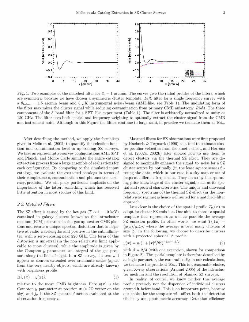
Fig. 1. Two examples of the matched filter for θc = 1 arcmin. The curves give the radial profiles of the filters, whichare symmetric because we have chosen a symmetric cluster template. Left: filter for a single frequency survey witha θfwhm = 1.5 arcmin beam and 8 µK instrumental noise/beam (AMI–like, see Table 1). The undulating form ofthe filter maximizes the cluster signal while reducing contamination from primary CMB anisotropy. Right: The threecomponents of the 3–band filter for a SPT–like experiment (Table 1). The filter is arbitrarily normalized to unity at150 GHz. The filter uses both spatial and frequency weighting to optimally extract the cluster signal from the CMBand instrument noise. Although in this Figure the filters continue to large radii, in practice we truncate them at 10θc.

After describing the method, we apply the formalismgiven in Melin et al. (2005) to quantify the selection func-tion and contamination level in up–coming SZ surveys.We take as representative survey configurations AMI, SPTand Planck, and Monte Carlo simulate the entire catalogextraction process from a large ensemble of realizations foreach configuration. By comparing to the simulated inputcatalogs, we evaluate the extracted catalogs in terms oftheir completeness, contamination and photometric accu-racy/precision. We will place particular emphasis on theimportance of the latter, something which has receivedlittle attention in most studies of this kind.

2.2. Matched Filters

The SZ effect is caused by the hot gas (T ∼ 1 − 10 keV)contained in galaxy clusters known as the intraclustermedium (ICM); electrons in this gas up–scatter CMB pho-tons and create a unique spectral distortion that is nega-tive at radio wavelengths and positive in the submillime-ter, with a zero–crossing near 220 GHz. The form of thisdistortion is universal (in the non–relativistic limit appli-cable to most clusters), while the amplitude is given bythe Compton y parameter, an integral of the gas pres-sure along the line–of–sight. In a SZ survey, clusters willappear as sources extended over arcminute scales (apartfrom the very nearby objects, which are already known)with brightness profile

∆iν(x) = y(x)jν (1)

relative to the mean CMB brightness. Here y(x) is theCompton y parameter at position x (a 2D vector on thesky) and jν is the SZ spectral function evaluated at theobservation frequency ν.

Matched filters for SZ observations were first proposedby Haehnelt & Tegmark (1996) as a tool to estimate clus-ter peculiar velocities from the kinetic effect, and Herranzet al. (2002a, 2002b) later showed how to use them todetect clusters via the thermal SZ effect. They are de-signed to maximally enhance the signal–to–noise for a SZcluster source by optimally (in the least square sense) fil-tering the data, which in our case is a sky map or set ofmaps at different frequencies. They do so by incorporat-ing prior knowledge of the cluster signal, such as its spa-tial and spectral characteristics. The unique and universalfrequency spectrum of the thermal SZ effect (in the non–relativistic regime) is hence well suited for a matched–filterapproach.

Less clear is the choice of the spatial profile Tθc(x) toadopt for cluster SZ emission. One aims to choose a spatialtemplate that represents as well as possible the averageSZ emission profile. In other words, we want Tθc(x) =〈y(x)/yo〉C , where the average is over many clusters ofsize θc. In the following, we choose to describe clusterswith a projected spherical β–profile:

y(x) = yo(1 + |x|2/θ2c)−(3β−1)/2 (2)

with β = 2/3 (with one exception, shown for comparisonin Figure 2). The spatial template is therefore described bya single parameter, the core radius θc; in our calculations,we truncate the profile at 10θc. This is a reasonable choice,given X–ray observations (Arnaud 2005) of the intraclus-ter medium and the resolution of planned SZ surveys.

In reality, of course, we know neither this averageprofile precisely nor the dispersion of individual clustersaround it beforehand. This is an important point, becauseour choice for the template will affect both the detectionefficiency and photometric accuracy. Detection efficiency


will be reduced if the template does not well represent theaverage profile and, as will become clear below, the pho-tometry will be biased. In general, the survey selection

function unavoidably suffers from uncertainty induced by

unknown source astrophysics (in addition to other sourcesof uncertainty).

In the following, we first study (Section 4) the idealcase where the filters perfectly match the cluster profiles,i.e., we use the β–model for both our simulations and asthe detection template. In a later section (5), we examinethe effects caused by non–trivial cluster morphology, aswell as by point source confusion.

Consider a cluster with core radius θc and central y–value yo positioned at an arbitrary point xo on the sky. Forgenerality, suppose that the region is covered by severalmaps Mi(x) at N different frequencies νi (i = 1, ..., N).We arrange the survey maps into a column vector M(x)whose ith component is the the map at frequency νi; thisvector reduces to a scalar map in the case of a single fre-quency survey. Our maps contain the cluster SZ signalplus noise:

M(x) = yojνTθc(x− xo) + N (x) (3)

where N is the noise vector (whose components are noisemaps at the different observation frequencies) and jν isa vector with components given by the SZ spectral func-tion jν evaluated at each frequency. Noise in this con-text refers to both instrumental noise as well as all signalsother than the cluster thermal SZ effect; it thus also com-prises astrophysical foregrounds, for example, the primaryCMB anisotropy, diffuse Galactic emission and extragalac-tic point sources.

We now build a filter Ψθc(x) (in general, a column

vector in frequency space) that returns an estimate, yo, ofyo when centered on the cluster:

yo =

∫

d2x Ψθc

t(x− xo) ·M(x) (4)

where superscript t indicates a transpose (with complexconjugation when necessary). This is just a linear com-bination of the maps, each convolved with its frequency–specific filter (Ψθc)i. We require an unbiased estimate ofthe central y value, so that 〈yo〉 = yo, where the aver-age here is over both total noise and cluster (of core ra-dius θc) ensembles. Building the filter with the known SZspectral form and adopted spatial template optimizes thesignal–to–noise of the estimate; in other words, the fil-ter is matched to the prior information. The filter is nowuniquely specified by demanding a minimum variance es-timate. The result expressed in Fourier space (the flat skyapproximation is reasonable on cluster angular scales) is(Haehnelt & Tegmark 1996, Herranz et al. 2002a, Melinet al. 2005):

Ψθc(k) = σ2

θcP−1(k) · Fθc

(k) (5)

where

Fθc(k) ≡ jνTθc(k) (6)

Fig. 2. Filter noise expressed in terms of integrated SZflux Y – σY = σθc

∫

Tθc(x) dx – as a function of templatecore radius θc for the three experiments listed in Table 1.A cluster with Y = σY would be detected at a signal–to–noise ratio q = 1. At a fixed detection threshold q (e.g.,3 or 5), the completeness of a survey rapidly increasesfrom zero to unity in the region above its correspondingcurve qσY(θc) (Melin et al. 2005). All the curves adopt ourfiducial value of β = 2/3, except the dashed–triple–dottedred curve, shown for comparison, which corresponds to theSPT case with β = 0.6; this curve is systematically higherby (2.5 to 13)%, depending on θc.

σθc ≡[∫

d2k Fθc

t(k) · P−1 · Fθc(k)

]−1/2

(7)

with P (k) being the noise power spectrum, a matrixin frequency space with components Pij defined by〈Ni(k)N∗

j (k′)〉N = Pij(k)δ(k−k′). The quantity σθc givesthe total noise variance through the filter. When we speakof the signal–to–noise of a detection, we refer to yo/σθc .

We write the noise power spectrum as a sum Pij =

P noisei δij + Bi(k)B∗

j (k)P skyij , where P noise

i represents theinstrumental noise power in band i, B(k) the observa-

tional beam and P skyij gives the foreground power (non–

SZ signal) between channels i and j. As explicitly writ-ten, we assume uncorrelated instrumental noise betweenobservation frequencies. Note that we treat the astrophysi-cal foregrounds as isotropic, stationary random fields withzero mean. The zero mode is, in any case, removed fromeach of the maps, and the model certainly applies to theprimary CMB anisotropy. It should also be a reasonablemodel for fluctuations of other foregrounds about theirmean, at least over cluster scales4.

Two examples of the matched filter for θc = 1 arcminare shown in Fig. 1, one for an AMI–like single frequencysurvey with a 1.5 arcmin beam (left–hand panel) and theother for a SPT–like 3–band filter (right–hand panel); see

4 Wemake no assumption about the Gaussianity of the fields;the estimator remains unbiased even if they are not Gaussian,although optimality must be redefined in this case.


Table 1 for the experimental characteristics. The filters arecircularly symmetric, with the figures giving their radialprofiles, because we have chosen a spherical cluster model.We clearly see the spatial weighting used by the singlefrequency filter to optimally extract the cluster from thenoise and CMB backgrounds. The multiple frequency filterΨθc

is a 3–element column vector containing filters foreach individual frequency. In this case, the filter employsboth spectral and spatial weighting to optimally extractthe cluster signal.

Figure 2 shows the filter noise as a function of tem-plate core radius θc. We plot the filter noise expressed interms of an equivalent noise σY ≡ σθc

∫

Tθc(x) dx on theintegrated SZ flux Y . The dashed–triple–dotted red curvewith β = 0.6 is shown for comparison to gauge the impactof changing this parameter, otherwise fixed at β = 2/3throughout this work. Melin et al. (2005) use the informa-tion in this figure to construct survey completeness func-tions. At fixed signal–to–noise q, the completeness of asurvey rapidly increases to unity in the region above thecurve qσY. The Figure shows that high angular resolutionground–based surveys (e.g., AMI, SPT) are not purelyflux limited, because their noise level rises significantlywith core radius. The lower resolution of the Planck sur-vey, on the other hand, results in more nearly flux limitedsample.

3. Catalog Extraction

Catalog construction proceeds in three steps, the last twoof which are repeated5:

1. Convolution of the frequency map(s) with matched fil-ters corresponding to different cluster sizes;

2. Identification of candidate clusters as objects withsignal–to–noise yo/σθc > q, where q is our fixed detec-tion threshold, followed by photometry of the bright-est remaining cluster candidate, which is then addedto the final cluster catalog;

3. Removal of this object from the set of filtered maps us-ing the photometric parameters (e.g., yo and θc) fromthe previous step.

We loop over the last two steps until there are no remain-ing candidates above the detection threshold. The follow-ing sections detail each step.

3.1. Map filtering

In the first step, we convolve the observed map(s)with matched filters covering the expected range of

5 Note that we have made some changes in the two last stepscompared to the description given in Melin et al. (2005). We nolonger sort candidates in a tree structure for de-blending; in-stead, we identify and then remove candidates one by one fromthe filtered maps. This has only a small impact on the com-pleteness of the detection algorithm, leaving the conclusionsof our previous paper intact. The changes, however, greatlyimprove photometry and lower contamination.

core radii. For AMI and SPT, for example, we varyθc from 0.1 to 3 arcmins in 0.1 steps (i.e., θc =0.1, 0.2, ..., 2.9, 3 arcmins) and add three values for thelargest clusters: 4, 5, 6 arcmins. We thus filter the map(s)nθc times (nθc = 33 for AMI and SPT) to obtain 2nθc

filtered maps, Jθc et Lθc . The nθc maps Jθc give the SZamplitude (obtained using Ψθc), while the nθc maps Lθc

give the signal–to–noise ratio: Lθc = Jθc/σθc). We set adetection threshold at fixed signal–to–noise q and identifycandidates at each filter scale θc as pixels with Lθc > q.Common values for the threshold are q = 3 and q = 5; thechoice is a tradeoff between detection and contaminationrates (see below).

3.2. Cluster parameter estimation: Photometry

We begin the second step by looking for the brightest can-didate pixel in the set of maps Lθc . The candidate clusteris assigned the spatial coordinates (x, y) of this pixel, andits core radius is defined as the filter scale of the mapcontaining the pixel: θc = θf . We then calculate the to-tal integrated flux using Y = yo

∫

Tθc(x) dx, where yo istaken from the map Jθc at the same filter scale. We referto this step as the photometric step, and the parametersyo, θc and Y as photometric parameters. Note that mea-surement error on Y comes from errors on both yo and θc(We return to this in greater detail in Section 4.4).

3.3. Catalog construction

The candidate cluster is now added to the final clustercatalog, and we proceed by removing it from the set offiltered maps Jθc and Lθc before returning to step 2. Tothis end, we construct beforehand a 2D array (library) ofun–normalized, filtered cluster templates (postage–stampmaps)

Tθc,θf (x) =

∫

d2x′ Ψθf (x′ − x)Tθc(x

′) (8)

with the cluster centered in the map. Note that θc runsover core radius and θf over filter scale. At each filter scaleθf , we place the normalized template yoTθc,θf on the clusterposition (x, y) and subtract it from the map. The libraryof filtered templates allows us to perform this step rapidly.

We then return to step 2 and repeat the process un-til there are no remaining candidate pixels. Thus, clustersare added to the catalog while being subtracted from themaps one at a time, thereby de-blending the sources. Bypulling off the brightest clusters first, we aim to mini-mize uncertainty in the catalog photometric parameters.Nevertheless, it must be emphasized that the entire pro-cedure relies heavily on the use of templates and that realclusters need not conform to the chosen profiles. We returnto the effects of cluster morphology below.

In the end, we have a cluster catalog with positions(x, y), central Compton y parameters, sizes θc and fluxesY .


Type Frequencies Res. fwhm Inst. noise Area[GHz] [arcmin] [µK/beam] [deg2]

AMI 15 1.5 8 10

SPT 150 1 10220 0.7 60 4000275 0.6 100

Planck 143 7.1 6217 5 13 41253353 5 40

Table 1. Characteristics of the three types of experimentsconsidered. We run our extraction method on 100 skypatches of 3 × 3 square degrees (for AMI and SPT) and12 × 12 square degrees (for Planck).

4. Cluster recovery

We tested our catalog construction method on simulatedobservations of the three representative types of SZ sur-vey specified in Table 1. The simulations include SZ emis-sion, primary CMB anisotropy and instrumental noise andbeam smearing. We do not include diffuse Galactic fore-grounds in this study. We begin in this section with theideal case where the filter perfectly matches the simulatedclusters (spherical β–model profiles) and in the absence ofextragalactic point sources. We return to the additionaleffects of cluster morphology and point source confusionin Section 5.

The simulated maps are generated by Monte Carlo. Wefirst create a realization of the linear matter distributionin a large box using the matter power spectrum. Clustersare then distributed according to their expected numberdensity, given by the mass function, and bias as a functionof mass and redshift. We also give each cluster a peculiarvelocity consistent with the matter distribution accord-ing to linear theory. The simulations thus featuring clus-ter spatial and velocity correlations accurate first order,which is a reasonable approximation on cluster scales. Inthis paper, we use these simulations but we do not studythe impact of the correlations on the detection method,leaving this issue to forthcoming work.

The cluster gas is modeled by a spherical isothermalβ–profile with β = 2/3 and θc/θv = 0.1, where θv is the an-gular projection of the virial radius and which varies withcluster mass and redshift following a self-similar relation-ship. We choose an M −T relation consistent with the lo-cal abundance of X–ray clusters and our value of σ8, givenbelow (Pierpaoli et al. 2004). Finally, we fix the gas massfraction at fgas = 0.12 (e.g., Mohr et al. 1999). The inputcatalog consists of clusters with total mass M > 1014M⊙,which is sufficient given the experimental characteristicslisted in Table 1. Delabrouille et al. (2002) describe thesimulation method in more detail.

We generate primary CMB anisotropies us-ing the power spectrum calculated by CMBFAST6

(Seljak & Zaldarriaga 1996) for a flat concordance model

6 http://cmbfast.org/

with ΩM = 0.3 = 1 − ΩΛ (Spergel et al. 2003), Hubbleconstant Ho = 70 km/s/Mpc (Freedman et al. 2001) anda power spectrum normalization σ8 = 0.98. As a laststep we smooth the map with a Gaussian beam and addGaussian white noise to model instrumental effects7.

We simulate maps that would be obtained from theproposed surveys listed in Table 1. The first is anAMI8–like experiment (Jones et al. 2002), a single fre-quency, high resolution interferometer; the sensitivitycorresponds to a one–month integration time per 0.1square degree (Kneissl et al. 2001). The SPT9–like exper-iment (Ruhl et al. 2004) is a high resolution, multi–bandbolometer array. We calculate the noise levels assuming anintegration time of 1 hour per square degree, and a splitof 2/3, 1/6, 1/6 of the 150, 220, 275 GHz channels for the1000 detectors in the focal plane array (Ruhl et al. 2004).Finally, we consider the space–based Planck10–like exper-iment, with a nominal sensitivity for a 14 month mission.For the AMI and SPT maps we use pixels11 of 30 arcsec,while for Planck the pixels are 2.5 arcmin.

We simulate 100 sky patches of 3 × 3 square degreesfor both AMI and SPT, and of 12 × 12 square degreesfor Planck. This is appropriate given the masses of de-tected clusters in each experiment. In practice, AMI willcover a few square degrees, similar to the simulated patch,while SPT will cover 4000 square degrees and Planck willobserve the entire sky. Thus, the surveys decrease in sen-sitivity while increasing sky coverage from top to bottomin Table 2 (see also Table 1).

deg−2 S/N > 3 S/N > 5

AMI 44 20(38) (16)

SPT 35 12(27) (11)

Planck 1.00 0.38(0.84) (0.35)

Table 2. Extracted counts/sq. deg. from simulations ofthe three types of survey. The numbers in parenthesis givethe counts predicted by our analytic cluster model; thedifference is due to cluster overlap confusion (see text).

7 The 3–year WMAP results, published after the work pre-sented here was finished, favor a significantly lower value ofσ8 (Spergel et al. 2006). This could lower the total number ofclusters in our simulations by up to a factor of ∼ 2. As weare interested here in catalog recovery, where we compare out-put to input catalogs, this change should only cause relativelyminor changes to our final results.

8 http://www.mrao.cam.ac.uk/telescopes/ami/index.html9 http://astro.uchicago.edu/spt/

10 http://www.rssd.esa.int/index.php?project=PLANCK11 Pixel sizes are at least 2 times smaller than the best channelof each experiment.

http://cmbfast.org/

http://www.mrao.cam.ac.uk/telescopes/ami/index.html

http://astro.uchicago.edu/spt/

http://www.rssd.esa.int/index.php?project=PLANCK


Fig. 3. Cluster counts N(> Y ) per square degree as afunction of true SZ flux Y for a threshold of S/N > 5. Thedash–dotted black line gives the cluster counts from themass function (Jenkins et al. 2001). The dashed blue linegives the recovered cluster counts for AMI, the red solidline for SPT and the dotted green line for Planck. Theinset shows the completeness ratio (relative to the massfunction prediction) for each survey. All the surveys aresignificantly incomplete at their point–source sensitivities(5 times the y–intercept in Figure 2).

4.1. Association criteria

An important issue for catalog evaluation is the associa-tion between a detected object (candidate cluster) with acluster from the simulation input catalog (real cluster); inother words, a candidate corresponds to which, if any, realcluster. Any association method will be imprecise, and es-timates of catalog completeness, contamination and pho-tometric accuracy will unavoidably depend on the choiceof association criteria.

We proceed as follows: for each detection, we look atall input clusters with centers positioned within a distancer =

√8 × d, where d is the pixel size (d = 30 arcsec for

AMI and SPT, d = 2.5 arcmin for Planck); this covers theneighboring 24 pixels. If there is no input cluster, then wehave a false detection; otherwise, we identify the candi-date with the cluster whose flux is closest to that of thedetection. After running through all the candidates in thisfashion, we may find that different candidates are associ-ated with the same input cluster. In this case, we onlykeep the candidate whose flux is closest to the commoninput cluster, and we flag the other candidates as falsedetections (multiple detections).

At this stage, some associations may nevertheless bechance alignments. We therefore employ a second param-eter, Ycut: a candidate associated with a real cluster offlux Y < Ycut is flagged as a false detection. We indicatethese false detections as diamonds in Figures 7, 8, 9 and11. The idea is that such clusters are too faint to havebeen detected and the association is therefore by chance.In the following, we take Ycut = 1.5 × 10−5 arcmin2 for

AMI and SPT, respectively, and Ycut = 3 × 10−4 arcmin2

for Planck. Note that these numbers are well below thepoint–source sensitivity (at S/N=5) in each case (see be-low and Figure 2).

4.2. Completeness

Figure 3 shows completeness for the three experimentsin terms of true integrated Y , while Table 2 summarizesthe counts. In Figure 4 we give the corresponding limitingmass as a function of redshift. Given our cluster model,AMI, SPT and Planck should find, respectively, about 16,11 and 0.35 clusters/deg.2 at a S/N > 5; these are thenumbers given in parentheses in Table 2. Cluster overlapconfusion accounts for the fact that the actual counts ex-tracted from the simulated surveys are higher: some clus-ters that would not otherwise pass the detection cut enterthe catalog because the filter adds in flux from close neigh-bors.

A detection threshold of S/N = 5 correspondsto a point–source sensitivity of just below Y = 5 ×10−5 arcmin2 for both AMI and SPT, as can be read offthe left–hand–side of Figure 2. The surveys approach ahigh level of completeness only at Y > 10−4 arcmin2,however, due to the rise of the selection cut with core ra-dius seen in Figure 2. For these high resolution surveys,point–source sensitivity gives a false idea of the surveycompleteness flux limit.

At the same signal–to–noise threshold, Planck is essen-tially complete above Y ∼ 10−3 arcmin2 and should detectabout 0.4 clusters per square degree. Since most clustersare unresolved by Planck, the survey reaches a high com-pleteness level near the point–source sensitivity. We alsosee this from the small slope of the Planck selection cutin Figure 2.

We emphasize that the surveys (in particular, thehigh resolution surveys) are not flux limited for anyvalue of q, because increasing q simply translates thecurve in Figure 2 along the y axis. However, one canapproach a flux–limited catalog by selecting clusters atS/N > q and then cutting the resulting catalog atYo > Ylimit ≡ QσY (θc = 0.1 arcmin), where the constantQ > q. As Q increases we tend towards a catalog for whichY ∼ Yo > Ylimit. In the case of SPT with q = 3, for ex-ample, we find that large values of Q (> 10) are requiredto approach a reasonable flux–limited catalog; this con-struction, however, throws away a very large number ofdetected clusters.

Although the AMI (single frequency) and SPT (multi-band) survey maps have comparable depth, SPT will cover∼ 4000 sq. degrees, compared to AMI’s ∼ 10 sq. degrees.Planck will only find the brightest clusters, but with fullsky coverage. Predictions for the counts suffer from clus-ter modeling uncertainties, but the comparison betweenexperiments is robust and of primary interest here.


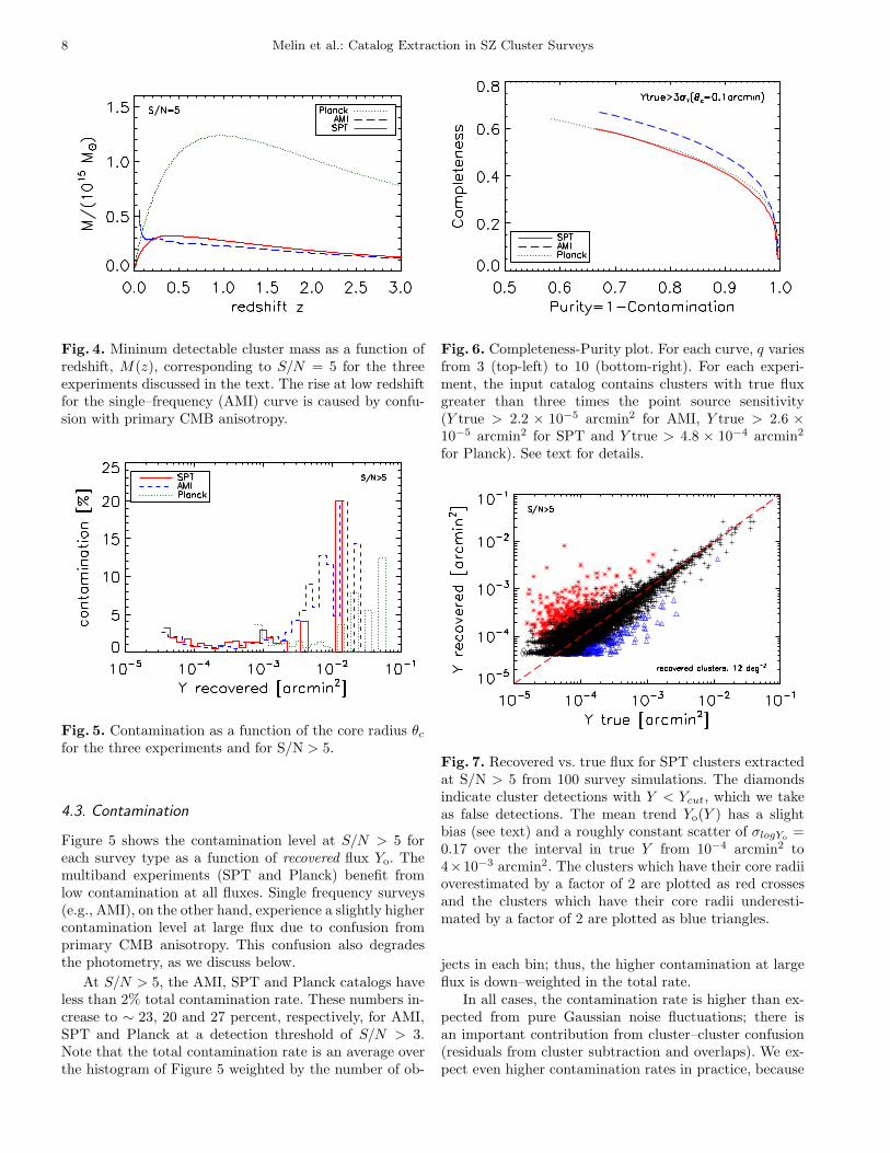
Fig. 4. Mininum detectable cluster mass as a function ofredshift, M(z), corresponding to S/N = 5 for the threeexperiments discussed in the text. The rise at low redshiftfor the single–frequency (AMI) curve is caused by confu-sion with primary CMB anisotropy.

Fig. 5. Contamination as a function of the core radius θcfor the three experiments and for S/N > 5.

4.3. Contamination

Figure 5 shows the contamination level at S/N > 5 foreach survey type as a function of recovered flux Yo. Themultiband experiments (SPT and Planck) benefit fromlow contamination at all fluxes. Single frequency surveys(e.g., AMI), on the other hand, experience a slightly highercontamination level at large flux due to confusion fromprimary CMB anisotropy. This confusion also degradesthe photometry, as we discuss below.

At S/N > 5, the AMI, SPT and Planck catalogs haveless than 2% total contamination rate. These numbers in-crease to ∼ 23, 20 and 27 percent, respectively, for AMI,SPT and Planck at a detection threshold of S/N > 3.Note that the total contamination rate is an average overthe histogram of Figure 5 weighted by the number of ob-

Fig. 6. Completeness-Purity plot. For each curve, q variesfrom 3 (top-left) to 10 (bottom-right). For each experi-ment, the input catalog contains clusters with true fluxgreater than three times the point source sensitivity(Y true > 2.2 × 10−5 arcmin2 for AMI, Y true > 2.6 ×10−5 arcmin2 for SPT and Y true > 4.8 × 10−4 arcmin2

for Planck). See text for details.

Fig. 7. Recovered vs. true flux for SPT clusters extractedat S/N > 5 from 100 survey simulations. The diamondsindicate cluster detections with Y < Ycut, which we takeas false detections. The mean trend Yo(Y ) has a slightbias (see text) and a roughly constant scatter of σlogYo

=0.17 over the interval in true Y from 10−4 arcmin2 to4×10−3 arcmin2. The clusters which have their core radiioverestimated by a factor of 2 are plotted as red crossesand the clusters which have their core radii underesti-mated by a factor of 2 are plotted as blue triangles.

jects in each bin; thus, the higher contamination at largeflux is down–weighted in the total rate.

In all cases, the contamination rate is higher than ex-pected from pure Gaussian noise fluctuations; there isan important contribution from cluster–cluster confusion(residuals from cluster subtraction and overlaps). We ex-pect even higher contamination rates in practice, because


of variations in cluster morphology around the filter tem-plates. We quantify this latter effect below.

A useful summary of these results is a completeness–purity plot, as shown in Figure 6. Proper comparison ofthe different experiments requires an appropriate choice ofinput catalog used to define the completeness in this plot.Here, we take the input catalog as all clusters with (true)flux geater than three times the point source sensitivity foreach experiment. If the clusters were point sources and thedetection method perfect (i.e. not affected by confusion),the completeness would be 1 for q = 3 in the top-left cor-ner. These curves summarize the efficiency of our clusterdetection method; however, they give no information onthe photometric capabilities of the experiments.

4.4. Photometry

We now turn to the important, but often neglected is-sue of cluster SZ photometry. The ability of a SZ sur-vey to constrain cosmology relies on application of theY − M relation. As mentioned, we expect the intrin-

sic (or true) flux to tightly correlate with cluster mass(Bartlett 2001), as indeed borne out by numerical simula-tions (da Silva et al. 2004, Motl et al. 2005, Nagai 2005).Nevertheless, unknown cluster physics could affect theexact form and normalization of the relation, pointingup the necessity of an empirical calibration (referred toas survey calibration), either with the survey data it-self (self–calibration, Hu 2003, Majumdar & Mohr 2003,Lima & Hu 2004, Lima & Hu 2005) or using externaldata, such as lensing mass estimates (Bartelmann 2001)(although the latter will be limited to relatively low red-shifts).

Photometric measurement accuracy and precision is asimportant as cluster physics in this context: what mattersin practice is the relation between recovered SZ flux Yo

and cluster mass M . Biased SZ photometry (bias in theY − Yo) relation will change the form and normalizationof the Yo −M relation and noise will increase the scatter.One potentially important source of photometric error forthe matched filter comes from cluster morphology, i.e., thefact that cluster profiles do not exactly follow the filtershape (see Section 5).

Survey calibration will help remove the bias, but withan ease that depends on the photometric scatter: largescatter will increase calibration uncertainty and/or neces-sitate a larger amount of external data. In addition, scat-ter will degrade the final cosmological constraints (e.g.,Lima & Hu 2005). Photometry should therefore be con-sidered an important evaluation criteria for cluster catalogextraction methods.

Consider, first, SPT photometry. Figure 7 shows therelation between observed (or recovered) flux Yo and trueflux Y for a detection threshold of S/N > 5. Fitting forthe average trend of Yo as a function of Y , we obtain

logYo = 0.96logY − 0.15

Fig. 8. Recovered vs. true flux for Planck clusters ex-tracted at S/N > 5 from 100 survey simulations. The di-amonds indicate cluster detections with Y < Ycut, whichwe take as false detections. The mean trend Yo(Y ) hasa slight bias (see text) and a roughly constant scat-ter of σlogYo

= 0.13 over the interval in true Y from2 × 10−3 arcmin2 to 2 × 10−2 arcmin2.The clusters whichhave their core radii overestimated by a factor of 2 areplotted as red crosses and the clusters which have theircore radii underestimated by a factor of 2 are plotted asblue triangles.

over the interval 10−4 arcmin2 < Y < 4 × 10−3 arcmin2,with Yo and Y measured in arcmin2. There is a slight biasin that the fit deviates somewhat from the equality line,but the effect is minor. Below this flux interval, the fit curlsupward in a form of Malmquist bias caused by the S/Ncut (seen as the sharp lower edge on Yo). The lack of anysignificant bias is understandable in this ideal case wherethe filter perfectly matches the cluster SZ profile. Clustermorphology, by which we mean a mismatch between thecluster SZ profile and the matched filter template), caninduce bias; we return to this issue in Section 5.

The scatter about the fit is consistent with a Gaussiandistribution with a roughly constant standard deviationof σlogYo

= 0.17 over the entire interval.The scatter is a factor of 10 larger than expected from

instrumental noise alone, which is given by the selectioncurve in Figure 2. Uncertainty in the recovered clusterposition, core radius and effects from cluster–cluster con-fusion all strongly influence the scatter. Photometry pre-cision, therefore, cannot be predicted from instrumentalnoise properties alone, but only with simulations account-ing for these other, more important effects.

Figure 8 shows the photometry for the Planck survey.Apart from some catastrophic cases (the diamonds), thephotometry is good and fit by

logYo = 0.98logY − 0.07

over the interval 2×10−3 arcmin2 < Y < 2×10−2 arcmin2

(Yo, Y measured in arcmin2). The dispersion is σlogYo=


0.13, roughly constant over the same interval. For unre-solved clusters, this scatter is ∼ 5 times larger than theexpected instrumental–induced scatter. The brightest di-amonds in the Figure correspond to real clusters with po-sitional error larger than the association criteria r. As aconsequence, the candidates are falsely associated with asmall, nearby cluster, unrelated to the actual detected ob-ject.

We emphasize that the observational scatter in theYo − Y relation for both SPT and Planck dominates theintrinsic scatter of less than 5% seen in the Y − M re-lation from numerical simulations (da Silva et al. 2004,Motl et al. 2005).

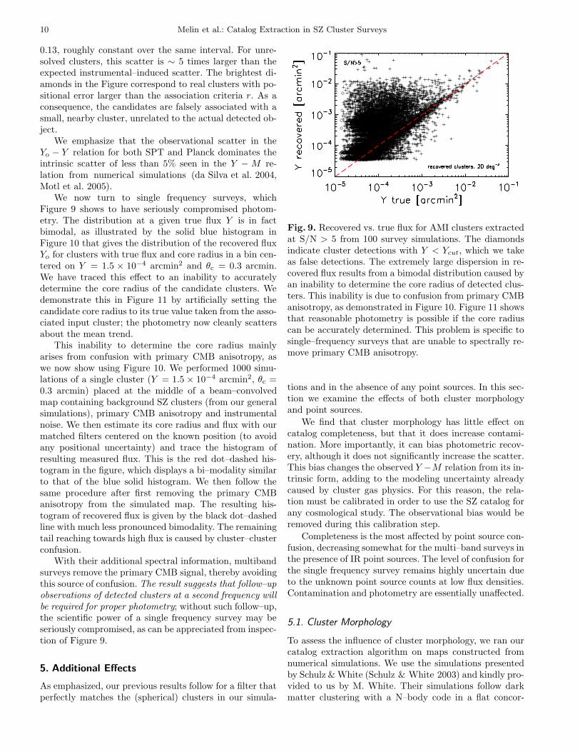
We now turn to single frequency surveys, whichFigure 9 shows to have seriously compromised photom-etry. The distribution at a given true flux Y is in factbimodal, as illustrated by the solid blue histogram inFigure 10 that gives the distribution of the recovered fluxYo for clusters with true flux and core radius in a bin cen-tered on Y = 1.5 × 10−4 arcmin2 and θc = 0.3 arcmin.We have traced this effect to an inability to accuratelydetermine the core radius of the candidate clusters. Wedemonstrate this in Figure 11 by artificially setting thecandidate core radius to its true value taken from the asso-ciated input cluster; the photometry now cleanly scattersabout the mean trend.

This inability to determine the core radius mainlyarises from confusion with primary CMB anisotropy, aswe now show using Figure 10. We performed 1000 simu-lations of a single cluster (Y = 1.5 × 10−4 arcmin2, θc =0.3 arcmin) placed at the middle of a beam–convolvedmap containing background SZ clusters (from our generalsimulations), primary CMB anisotropy and instrumentalnoise. We then estimate its core radius and flux with ourmatched filters centered on the known position (to avoidany positional uncertainty) and trace the histogram ofresulting measured flux. This is the red dot–dashed his-togram in the figure, which displays a bi–modality similarto that of the blue solid histogram. We then follow thesame procedure after first removing the primary CMBanisotropy from the simulated map. The resulting his-togram of recovered flux is given by the black dot–dashedline with much less pronounced bimodality. The remainingtail reaching towards high flux is caused by cluster–clusterconfusion.

With their additional spectral information, multibandsurveys remove the primary CMB signal, thereby avoidingthis source of confusion. The result suggests that follow–up

observations of detected clusters at a second frequency will

be required for proper photometry; without such follow–up,the scientific power of a single frequency survey may beseriously compromised, as can be appreciated from inspec-tion of Figure 9.

5. Additional Effects

As emphasized, our previous results follow for a filter thatperfectly matches the (spherical) clusters in our simula-

Fig. 9. Recovered vs. true flux for AMI clusters extractedat S/N > 5 from 100 survey simulations. The diamondsindicate cluster detections with Y < Ycut, which we takeas false detections. The extremely large dispersion in re-covered flux results from a bimodal distribution caused byan inability to determine the core radius of detected clus-ters. This inability is due to confusion from primary CMBanisotropy, as demonstrated in Figure 10. Figure 11 showsthat reasonable photometry is possible if the core radiuscan be accurately determined. This problem is specific tosingle–frequency surveys that are unable to spectrally re-move primary CMB anisotropy.

tions and in the absence of any point sources. In this sec-tion we examine the effects of both cluster morphologyand point sources.

We find that cluster morphology has little effect oncatalog completeness, but that it does increase contami-nation. More importantly, it can bias photometric recov-ery, although it does not significantly increase the scatter.This bias changes the observed Y −M relation from its in-trinsic form, adding to the modeling uncertainty alreadycaused by cluster gas physics. For this reason, the rela-tion must be calibrated in order to use the SZ catalog forany cosmological study. The observational bias would beremoved during this calibration step.

Completeness is the most affected by point source con-fusion, decreasing somewhat for the multi–band surveys inthe presence of IR point sources. The level of confusion forthe single frequency survey remains highly uncertain dueto the unknown point source counts at low flux densities.Contamination and photometry are essentially unaffected.

5.1. Cluster Morphology

To assess the influence of cluster morphology, we ran ourcatalog extraction algorithm on maps constructed fromnumerical simulations. We use the simulations presentedby Schulz & White (Schulz & White 2003) and kindly pro-vided to us by M. White. Their simulations follow darkmatter clustering with a N–body code in a flat concor-


Fig. 10. The full blue histogram gives the cluster countsfrom figure 9 in the bin (10−4 < Y < 2.10−4, 0.25 < θc <0.35). We have added the cluster counts obtained from thesize and flux estimation of a single cluster (Y = 1.5×10−4,θc = 0.3) at a known position through 1000 simulations.SZ cluster background maps and the instrumental beamand noise are included. Two cases are considered : withprimary CMB (dotted red histogram) and without pri-mary CMB (dash–dotted black line). The double bump inY recovery is visible when the primary CMB is presentand disappears when it’s removed showing that the pri-mary CMB power spectrum is the cause of the doublebump.

Fig. 11. Single–frequency photometry when we artificiallyset the core radii of detected clusters to their true valuesfrom the input catalog. The dispersion decreases dramati-cally, demonstrating that the inability to recover the coreradius is the origin of the bad photometry seen in Figure 9.

dance cosmology, and model cluster gas physics with semi–analytical techniques by distributing an isothermal gas ofmass fraction ΩB/ΩM according to the halo dark mat-ter distribution. For details, see Schulz & White. In thefollowing, we refer to these simulations as the “N–body”simulations.

Fig. 12. Photometry for the SPT catalog from the N–body simulations. Cluster morphology (mismatch betweenthe filter profile and the actual cluster SZ profile) clearlyinduces a bias between the recovered and true SZ flux.The scatter, on the other hand, is not very affected, ascan be seen in comparing with Figure 7.

We proceed by comparing catalogs extracted from theN–body map to those from a corresponding simulationmade with spherical clusters. The latter is constructed byapplying our spherical β–model gas distribution to thecluster halos taken from the N–body simulation and usingthem as input to our Monte Carlo sky maps. In the pro-cess, we renormalize our Y −M relation to the one used inthe N–body SZ maps. We thus obtain two SZ maps con-taining the same cluster halos, one with spherical clusters(referred to hereafter as the “β–model” maps) and theother with more complex cluster morphology (the N-bodymaps). Comparison of the catalogs extracted from the twodifferent types of simulated map gives us an indication ofthe sensitivity of our method to cluster morphology. Wemake this comparative study only for the SPT and Plancklike surveys.

Catalog completeness is essentially unaffected by clus-ter morphology; the integrated counts, for example, followthe same curves shown in Figure 3 with very little devi-ation, the only difference being a very small decrease inthe Planck counts at the lowest fluxes. The effect, for ex-ample, is smaller than that displayed in Figure 13 due topoint source confusion (and discussed below).

Non–trivial cluster morphology, however, does signifi-cantly increase the catalog contamination rate; for exam-ple, in the SPT survey the global contamination rises fromless than 2% to 13% at S/N = 5 for the N–body simula-tions. We trace this to residual flux left in the maps aftercluster extraction: cluster SZ signal that deviates fromthe assumed spherical β–model filter profile remains inthe map and is picked up later as new cluster candidates.Masking those regions where a cluster has been previouslyextracted (i.e., forbidding any cluster detection) drops thecontamination to 4% (SPT case), but causes a decrease


of 2.8 clusters per square degree in the recovered counts;this technique would also have important consequences forclustering studies.

From Figure 12, we clearly see that cluster morphologyinduces a bias in the photometry. This arises from the factthat the actual cluster SZ profiles differ from the templateadopted for the filter. The differences are of two types: anoverall difference in the form of radial profile and localdeviations about the average radial profile due to clustersubstructure. It is the former that is primarily responsi-ble for the bias. In our case, the N–body simulations havemuch more centrally peaked SZ emission than the filtertemplates, which causes the filter to systematically un-derestimate the total SZ flux. Cluster substructure willincrease the scatter about the mean Yo − Y relation. Thislatter effect is not large, at least for the N–body simula-tions used here, as can be seen by comparing the scatterin Figures 12 and 7.

We emphasize, however, that the quantitative effectson photometry depend on the intrinsic cluster profile, andhence are subject to modeling uncertainty. The simula-tions used here do not include gas physics and simply as-sume that the gas follows the dark matter. The real biaswill depend on unknown cluster physics, thus adding tothe modeling uncertainty in the Y −M relation. This un-certainty, due to both cluster physics and the photometricuncertainty discussed here, must be dealt with by empir-ically calibrating the relation, either with external data(lensing) and/or internally (self–calibration).

Fig. 13. Integrated cluster counts for the three types ofsurvey. The upper curve in each pair reproduces the re-sults of Figure 3, while the lower curve shows the effect ofpoint source confusion. Despite the large IR point sourcepopulation, multiband surveys efficiently eliminate confu-sion. The AMI–like survey is, on the other hand, stronglyaffected. This latter effect remains uncertain due to a lackof information on the faint end of the radio point sourcecounts (see text).

5.2. Point Sources

We next examine the effect of point sources. In a previouspaper (Bartlett & Melin 2005, hereafter BM) we studiedtheir influence on survey detection sensitivity. We extendthis work to our present study in this section.

Low frequency surveys, such as our AMI example, con-tend with an important radio source population, whilehigher frequency bolometer surveys face a large popula-tion of IR sources. Radio source counts down to the sub–mJy flux levels relevant for SZ surveys are unfortunatelypoorly known. The IR counts are somewhat better con-strained at fluxes dominating the fluctuations in the IRbackground, although at higher frequencies (850 microns)than those used in SZ surveys; an uncertain extrapolationin frequency is thus necessary.

For the present study, we use the radio counts fitby Knox et al. 2004 to a combination of data from CBI,DASI, VSA and WMAP (see also Eq. 6 in BM), and IRcounts fit to blank–field SCUBA observations at 850 mi-crons by Borys et al. 2003 (and given by Eq. 8 in BM). Wefurther assume that all radio sources brighter than 100 µJyhave been subtracted from our maps at 15 GHz (AMIcase); this is the target sensitivity of the long baseline RyleTelescope observations that will perform the source sub-traction for AMI. No such explicit point source subtrac-tion is readily available for the higher frequency bolometersurveys; they must rely solely on their frequency coverageto reduce point source confusion. We therefore include allIR sources in our simulations, and fix their effective spec-tral index α = 3 with no dispersion12. We refer the readerto BM for details of our point source model. Note thatfor this study we use the spherical cluster model for directcomparison to our fiducial results.

Figure 13 compares the integrated counts fromFigure 3 (upper curve in each case) to those extracted fromthe simulations including point sources (lower curves). Wesee that point source confusion only slightly decreases thecompleteness of the multiband surveys, but greatly affectsthe single frequency survey.

In the case of SPT, this is because point source con-fusion remains modest compared to the noise: the two arecomparable at 150 GHz, but the noise power rises morequickly with frequency than the confusion power (see BMfor details) – in other words, the noise is bluer than theconfusion. This is an important consideration when look-ing for the optimal allocation of detectors to the observa-tion bands.

For Planck, confusion power dominates at all frequen-cies, but the spectral coverage provides sufficient leverageto control it. In this light, it must be emphasized that weonly include three astrophysical signals (SZ, CMB & pointsources) in these simulations, so that three observationbands are sufficient. In reality, one will have to deal withother foregrounds, e.g., diffuse Galactic emission, whichwill require the use of additional observation bands.

12 As discussed in BM, any dispersion has only a small effecton survey sensitivity


The single frequency observations, on the other hand,are strongly affected. This is consistent with the estimatein BM (Eq. 15) placing confusion noise well above instru-mental noise for the chosen point source model and sourcesubtraction threshold. We emphasize the uncertainty inthis estimate, however: in BM we showed, for example,that a model with flattening counts has much lower sourceconfusion while remaining consistent with the observedcounts at high flux densities. The actual confusion levelremains to be determined from deeper counts at CMB fre-quencies (see Waldram et al. 2003, Waldram et al. 2004for recent deep counts at 15 GHz).

Contamination in the multiband surveys is practicallyunaffected by point source confusion. For AMI we actu-ally find a lower contamination rate, an apparent gain ex-plained by the fact that the catalog now contains only thebrighter SZ sources, due to the lowered sensitivity causedby point source confusion.

The photometry of the multiband surveys also showslittle effect from the point sources. Fits to the recoveredflux vs. true flux relation do not differ significantly fromthe no–source case, and the dispersion remains essentiallythe same. This is consistent with the idea that point sourceconfusion is either modest compared to the noise (SPT)or controlled by multiband observations (Planck).

6. Discussion and Conclusion

We have described a simple, rapid method based onmatched multi–frequency filters for extracting cluster cat-alogs from SZ surveys. We assessed its performance whenapplied to the three kinds of survey listed in Table 1. Therapidity of the method allows us to run many simulationsof each survey to accurately quantify selection effects andobservational uncertainties. We specifically examined cat-alog completeness, contamination rate and photometricprecision.

Figure 2 shows the cluster selection criteria in termsof total SZ flux and source size. It clearly demonstratesthat SZ surveys, in particular high resolution ground–bases surveys, will not be purely flux limited, somethingwhich must be correctly accounted for when interpretingcatalog statistics (Melin et al. 2005).

Figure 3 and Table 2 summarize the expected yieldfor each survey. The counts roll off at the faint end wellbefore the point–source flux limit (intercept of the curvesin Figure 2 multiplied by the S/N limit) even at the highdetection threshold of S/N=5; the surveys loose complete-ness precisely because they are not purely flux–limited.These yields depend on the underlying cluster model andare hence subject to non–negligible uncertainty. They arenonetheless indicative, and in this work we focus on thenature of observational selection effects for which the ex-act yields are of secondary importance.

At our fiducial S/N=5 detection threshold, overall cat-alog contamination remains below 5%, with some depen-dence on SZ flux for the single frequency survey (seeFigure 5). The overall contamination rises to between 20%

and 30% at S/N>3. We note that the contamination rateis always larger than expected from pure instrumentalnoise, pointing to the influence of astrophysical confusion.

We pay particular attention to photometric precision,an issue often neglected in discussions of the scientific po-tential of SZ surveys. Scatter plots for the recovered fluxfor each survey type are given in Figures 7, 8 and 9. In thetwo multiband surveys, the recovered SZ flux is slightly bi-ased, due to the flux cut, with a dispersion of σlogYo

= 0.17and σlogYo

= 0.13 for SPT and Planck, respectively. Thisobservational dispersion is significantly larger than the in-trinsic dispersion in the Y −M relation predicted by hy-drodynamical simulations. This uncertainty must be prop-erly accounted for in scientific interpretation of SZ cata-logs; specifically, it will degrade survey calibration andcosmological constraints.

Even more importantly, we found that astrophysi-cal confusion seriously compromises the photometry ofthe single frequency survey (Figure 9). The histogram inFigure 10 shows that the recovered flux has in fact a bi-modal distribution. We traced the effect to an inabilityto determine source core radii in the presence of primaryCMB anisotropy. If cluster core radius could be accuratelymeasured, e.g., with X–ray follow–up, then we would ob-tain photometric precision comparable to the multibandsurveys (see Figure 11). This confusion can also be re-moved by follow–up of detected sources at a second ra-dio frequency (e.g., 90 GHz). Photometric uncertainty willtherefore be key limiting factor in single frequency SZ sur-veys.

All these results apply to the ideal case where the filterexactly matches the (simulated) cluster profiles. We thenexamined the potential impact of cluster morphology andpoint sources on these conclusions.

Using N–body simulations, we found that cluster mor-phology has little effect on catalog completeness, but thatit does increase the contamination rate and bias the pho-tometry. The increased contamination is caused by de-viations from a smooth radial SZ profile that appear asresidual flux in the maps after source extraction. Moreimportantly, the photometry is biased by the mismatchbetween the filter template and the actual cluster profile.This observational bias adds to the modeling uncertaintyin the Y −M relation, which will have to be empiricallydetermined in order to use the catalog for cosmology stud-ies.

As shown by Figure 13, point sources decrease sur-vey completeness. The multiband surveys effectively re-duce IR point source confusion and suffer only a small de-crease. Radio source confusion, on the other hand, greatlydecreased the completeness of the single frequency sur-vey. This is consistent with the expectation that, for ouradopted radio point source model and source subtractionthreshold, point source confusion dominates instrumentalnoise. Modeling uncertainty here is, however, very large:radio source counts are not constrained at relevant fluxes(∼ 100 µJy), which requires us to extrapolate counts frommJy levels (see BM for a more detailed discussion).


Surveys based on the SZ effect will open a new win-dow onto the high redshift universe. They inherit theirstrong scientific potential from the unique characteristicsof the SZ signal. Full realization of this potential, however,requires understanding of observational selection effectsand uncertainties. Overall, multiband surveys appear ro-bust in this light, while single frequency surveys will mostlikely require additional observational effort, e.g., follow–up in other wavebands, to overcome large photometric er-rors caused by astrophysical confusion with primary CMBanisotropy.

Acknowledgements. We thank T. Crawford for useful com-ments on matched filters and information about SPT, and A.Schulz and M. White for kindly providing us with their N-body simulations. We are also grateful to the anonymous ref-eree for helpful and insightful comments. JBM wishes to thankL. Knox, the Berkeley Astrophysics group and E. Pierpaoli fordiscussions on the detection method, and D. Herranz and theSantander group for discussions on matched filters. JBM wassupported at UC Davis by the National Science Foundationunder Grant No. 0307961 and NASA under Grant No. NAG5–11098.

References

Angulo R., Baugh C.M., Frenk C.S. et al. 2005, MNRAS, 362,L25

Arnaud M., astro–ph/0508159Barbosa D., Bartlett J.G., Blanchard A., 1996, A&A, 314, 13Bartelmann M. 2001, A&A, 370, 754Birkinshaw M. 1999, Proc. 3K Cosmology, 476, American

Institute of Physics, Woodbury, p. 298Blanchard A. & Bartlett J.G. 1998, A&A 332, L49Bartlett J. G. 2001, review in ”Tracing cosmic evolution

with galaxy clusters” (Sesto Pusteria 3-6 July 2001), ASPConference Series in press, astro–ph/0111211

Bartlett J.G. & Melin, J.-B. 2005, submittedBenson, A.J., Reichardt, C., Kamionkowski, M. 2002, MNRAS,

331, 71Bertin E. & Arnouts S. 1996, A&A, 117, 393Borys C., Chapman S., Halpern M. & Scott D. 2003, MNRAS,

344, 385Carlstrom J. E., Holder G. P., Reese E. D. 2002, ARA&A, 40,

643Colafrancesco, S., Mazzotta, P., Vittorio, N. 1997, ApJ, 488,

566Cole S., Percival W.J., Peacock J.A. et al 2005, MNRAS, 362,

505Delabrouille J., Melin J.-B., Bartlett J.G. 2002, in

”AMiBA 2001: High-Z Clusters, Missing Baryons,and CMB Polarization”, ASP Conference Proceedings,astro-ph/0109186

da Silva A.C., Kay S.T., Liddle A.R. & Thomas P.A. 2004,MNRAS, 348, 1401

Diego J.M., Vielva P., Martnez-Gonzlez E., Silk J., Sanz J.L.2002, MNRAS, 336, 1351

Eisenstein D.J., Zehavi I., Hogg D.W. et al. 2005, ApJ, 633,560

Eke V.R., Cole S., Frenk C.S. & Patrick Henry P.J. 1998,MNRAS, 298 1145

Freedman W.L., Madore B.F., Gibson B.K. et al. 2001, ApJ,553, 47

Haehnelt, M. G. & Tegmark, M. 1996, MNRAS, 279, 545Haiman Z., Mohr J.J. & Holder G.P. 2000, ApJ, 553, 545Herranz D., Sanz J.L., Barreiro R.B., Martnez-Gonzlez E.

2002, ApJ, 580, 610Herranz D., Sanz J.L., Hobson M.P., Barreiro R.B., Diego J.M.,

Martnez-Gonzlez E., Lasenby A. N. 2002, MNRAS, 336,1057

Hobson M.P. & McLachlan C. 2003, MNRAS, 338, 765Holder G. P., Mohr, J. J., Carlstrom J. E., Evrard A. E., Leitch

E. M. 2000, ApJ, 544, 629Hu W. 2003, Phys. Rev. D., 67, 081304Huetsi G. 2005, A&A, 446, 43Jenkins A., Frenk C.S., White S.D.M. et al. 2001, MNRAS,

321, 372Jones M.E., Edge A.C., Grainge, K. et al. 2001, MNRAS, 357,

518Juin J.B., Yvon D., Refregier A. & Yeche C. 2005,

astro–ph/0512378Kneissl, R., Jones, M.E., Saunders, R. et al. 2001, MNRAS,

328, 783Knox L., Holder, G.P., Church S.E. 2004, ApJ, 612, 96Lima M. & Hu W. 2004, Phys Rev D70, 043504Lima M. & Hu W. 2005, Phys Rev D72, 043006Lopez-Caniego M., Herranz D., Sanz J.L., Barreiro R.B. 2005,

astro-ph/0503149Majumdar S. & Mohr J.J. 2004, ApJ 613, 41Melin J.-B., Bartlett J.G., Delabrouille J. 2005, A & A 429,

417-426.Mohr J. J., Mathiesen B., Evrard A. E. 1999, ApJ, 517, 627Motl P.M., Hallman E.J., Burns J.O. & Norman M.L. 2005,

ApJ, 623, L63Nagai D., astro–ph/0512208Oukbir J. & Blanchard A. 1992, A&A, 262, L21Pierpaoli E., Anthoine S., Huffenberger K., Daubechies I. 2004,

MNRAS, 359, 261Pires S., Juin, J.B., Yvon D. et al., 0508641Rosati, P., Borgani, S. & Norman C. 2002, ARA&A 40, 539Ruhl J.E. et al. 2004, astro-ph/0411122Schafer B.M., Pfrommer C., Hell R.M, Bartelmann M. 2004,

MNRAS, 370, 1713Schulz, A. E., White, M. 2003, ApJ, 586, 723Seljak U. & Zaldarriaga, M. 1996, ApJ, 469, 437,

astro–ph/9603033, www.cmbfast.orgSpergel D. N. et al. 2003, ApJ Supplement Series, 148, 175Spergel D. N. et al. 2006, astro–ph/0603449Sunyaev, R. A. & Zel’dovich, Ya. B. 1970,Comments

Astrophys. Space Phys., ComAp,2,66Sunyaev, R. A. & Zel’dovich, Ya. B. 1972, Comments

Astrophys. Space Phys., 4, 173Vale C. & White M. 2005, New Astronomy, 11, 207Voit G. M. 2004, astro–ph/0410173Waldram E. M. et al. 2003, MNRAS 342, 915Waldram E. M. & Pooley G. G. 2004, astro–ph/0407422Wang S., Khoury J., Haiman, Z. & May M. 2004, PhysRev,

D70, 12300Weller J. & Battye R. A. 2003, NewAR, 47, 775White M., 2003, ApJ, 597, 650

http://arxiv.org/abs/astro--ph/0508159


http://arxiv.org/abs/astro-ph/0109186









Documents

Catalog Extraction in SZ Cluster Surveys: a matched ﬁlter