Catadioptric Stereo Using Planar Mirrors - … Stereo Using Planar Mirrors 67 Figure 1. Stereo image formation with a single camera and two planar mirrors. A scene point P reﬂected

International Journal of Computer Vision 44(1), 65–79, 2001c© 2001 Kluwer Academic Publishers. Manufactured in The Netherlands.

Catadioptric Stereo Using Planar Mirrors

JOSHUA GLUCKMAN AND SHREE K. NAYARDepartment of Computer Science, Columbia University, New York, NY 10027

Received July 23, 1999; Revised January 12, 2001; Accepted April 23, 2001

Abstract. By using mirror reflections of a scene, stereo images can be captured with a single camera (catadioptricstereo). In addition to simplifying data acquisition single camera stereo provides both geometric and radiometricadvantages over traditional two camera stereo. In this paper, we discuss the geometry and calibration of catadioptricstereo with two planar mirrors. In particular, we will show that the relative orientation of a catadioptric stereo rigis restricted to the class of planar motions thus reducing the number of external calibration parameters from 6 to 5.Next we derive the epipolar geometry for catadioptric stereo and show that it has 6 degrees of freedom rather than7 for traditional stereo. Furthermore, we show how focal length can be recovered from a single catadioptric imagesolely from a set of stereo correspondences. To test the accuracy of the calibration we present a comparison to Tsaicamera calibration and we measure the quality of Euclidean reconstruction. In addition, we will describe a real-timesystem which demonstrates the viability of stereo with mirrors as an alternative to traditional two camera stereo.

Keywords: stereo vision, real-time stereo, sensors, catadioptric mirrors

1. Introduction

Optical systems consisting of a combination of refract-ing (lens) and reflecting (mirror) elements are calledcatadioptric systems (Hecht and Zajac, 1974). Stereois one area of computer vision which can benefit fromsuch systems. By using two or more mirrored surfaces,a stereo view can be captured by a single camera (cata-dioptric stereo). This has the following advantages overtraditional two camera stereo.

• Identical System Parameters: Lens, CCD and dig-itizer parameters such as blurring, lens distortions,focal length, spectral response, gain, offset, pixelsize, etc. are identical for the stereo pair. Havingidentical system parameters facilitates stereo match-ing.

• Ease of Calibration: Because only a single cameraand digitizer are used, there is only one set of intrinsiccalibration parameters. Furthermore, we will showthat the extrinsic calibration parameters are con-strained by planar motion. Together these constraints

reduce the total number of calibration parametersfrom 16 in traditional stereo to 10 in our case.

• Data Acquisition: Camera synchronization is not anissue because only a single camera is used. Stereodata can easily be acquired and conveniently storedwith a standard video recorder without the need tosynchronize multiple cameras.

With these advantages in mind, we have designed andimplemented a real-time catadioptric stereo systemwhich uses only a single camera and two planar mir-rors. In addition, we have analyzed the geometry andcalibration of stereo with planar mirrors placed in anarbitrary configuration.

2. Previous Work

Previously, several researchers have demonstrated theuse of both curved and planar mirrors to acquire stereodata. Curved mirrors have been primarily used to cap-ture a wide field of view. One of the first uses ofcurved mirrors for stereo was in Nayar (1988), where

66 Gluckman and Nayar

Nayar suggested a wide field of view stereo systemconsisting of a conventional camera pointed at twospecular spheres. A similar system using two convexmirrors, one placed on top of the other, was proposedby Southwell et al. (1996). However, in both these sys-tems the projection of the scene produced by the curvedmirrors is not from a single viewpoint. Violation of the“single viewpoint assumption” implies that the pinholecamera model can not be used, thus making calibrationand correspondence a more difficult task.

Nayar and Baker (1997) derived the class of mir-rors which produce a single view point when imagedby a camera. Later, Nene and Nayar (1998) presentedseveral different catadioptric stereo configurations us-ing a single camera with planar, parabolic, elliptic, andhyperbolic mirrors. A catadioptric stereo system usinghyperbolic mirrors was implemented by Chaen et al.(1997). Gluckman et al. (1998) demonstrated a real-time panoramic stereo system using two coaxial cata-dioptric cameras (with parabolic mirrors).

The use of planar mirrors to acquire multi-view datahas also been investigated. As pointed out by severalresearchers (Teoh and Zhang, 1984; Nishimoto andShirai, 1987; Murray, 1995), it is possible to reconstructa scene by imaging the scene reflection in a rotating pla-nar mirror. However, these systems require more thanone image and therefore a static scene. Mitsumoto et al.(1992) previously described a stereo method which im-ages an object and its reflections in a set of planar mir-rors. Here, the mirrors were used to obtain occlusionfree images of the object. A similar method was alsoproposed in Zhang and Tsui (1998). Planar mirrors ar-ranged in a pyramid can also be used to obtain omnirec-tional stereo data as shown by Kawanishi et al. (1998).Recently, Shashua suggested using catadioptric stereofor non-rigid stereo platforms (Shashua, 1998).

Most similar to our work, are systems which cap-ture stereo data with planar mirrors and one camera.Goshtasby and Gruver (1993) designed a single camerastereo system using a pair of planar mirrors connectedby a hinge, leaving one degree of freedom between themirrors. Their system required the hinge to be verticallyaligned and centered in the image.

In the context of active vision, Inaba et al. (1993)built a single camera stereo system using four planarmirrors. They pointed out that for active vision appli-cations, such as high speed 3-d tracking, perfect stereosynchronization is needed. Four mirrors were used sothat the vergence angle could be controlled by changingthe angle between two of the mirrors and gaze could be

directed in front of the camera. A similar four mirrorcatadioptric system was was described by Mathieu andDevernay (1995).

Although several catadioptric stereo designs havebeen proposed in the literature, there has been no sys-tematic analysis of the properties (geometric and radio-metric), benefits and applications of such systems. Inthis paper, we will discuss several calibration issues inregard to single camera stereo with planar mirrors, in-cluding the determination of relative orientation, epipo-lar geometry, and focal length. These results togetherprovide a theoretical foundation for planar catadioptricstereo. In addition, we will describe a real-time cata-dioptric stereo system which demonstrates the viabilityof stereo with mirrors as an alternative to traditional twocamera stereo.

3. Geometry and Calibration

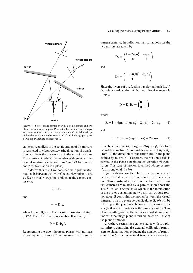
The results in this section pertain to the geometry andcalibration of catadioptric stereo systems that use a sin-gle perspective camera and two planar mirrors placedin an arbitrary configuration. Figure 1 depicts the imageformation of such a system. A scene point P is imagedas if seen from two different viewpoints v and v′. Thelocation of the two virtual pinholes is found by reflect-ing the camera pinhole c about each mirror. Reflectingthe optical axis of the camera about the mirrors deter-mines the optical axes and thus the orientations of thetwo virtual cameras. The focal length of each virtualcamera is equal to f , the focal length of the real cam-era. Therefore, the locations and orientations of the twovirtual cameras are determined by the orientations anddistances of the two mirrors with respect to the pinholeand optical axis of the camera.

We will derive both the relative orientation and theepipolar geometry of catadioptric stereo with two mir-rors. Then, we will discuss self-calibration constraintswhich can be used to recover the focal length solelyfrom a set of image correspondences. Finally, we ex-amine the field of view of two mirror stereo.

3.1. Relative Orientation

In traditional stereo, the two cameras can be placed inany configuration, and therefore the relative orienta-tion between the cameras is described by 6 parameters(3 for rotation and 3 for translation). For catadioptricstereo, the relative orientation between the two virtual

Catadioptric Stereo Using Planar Mirrors 67

Figure 1. Stereo image formation with a single camera and twoplanar mirrors. A scene point P reflected by two mirrors is imagedas if seen from two different viewpoints v and v′. With knowledgeof the relative orientation between v and v′ and the image pair p andp′, we can triangulate and recover P.

cameras, regardless of the configuration of the mirrors,is restricted to planar motion (the direction of transla-tion must lie in the plane normal to the axis of rotation).This constraint reduces the number of degrees of free-dom of relative orientation from 6 to 5 (3 for rotationand 2 for translation in a plane).

To derive this result we consider the rigid transfor-mation D between the two reflected viewpoints v andv′. Each virtual viewpoint is related to the camera cen-ter c as,

v = D1c

and

v′ = D2c,

where D1 and D2 are reflection transformations definedin (??). Then, the relative orientation D is simply,

D = D2D−11 .

Representing the two mirrors as planes with normalsn1 and n2 and distances d1 and d2 measured from the

camera center c, the reflection transformations for thetwo mirrors are given by

D1 =(

I − 2n1nT1 2d1n1

0 1

)

and

D2 =(

I − 2n2nT2 2d2n2

0 1

).

Since the inverse of a reflection transformation is itself,the relative orientation of the two virtual cameras issimply,

D = D2D1 =(

R t

0 1

)

where

R = I + 4(n1 · n2)n1nT2 − 2n1nT

1 − 2n2nT2 , (1)

and

t = 2d1n1 − (4d1(n1 · n2) + 2d2)n2. (2)

It can be shown that (n1 × n2) = R(n1 × n2), thereforethe rotation matrix R has a rotational axis of n1 × n2.From (2) the direction of translation lies in the planedefined by n1 and n2. Therefore, the rotational axis isnormal to the plane containing the direction of trans-lation. This type of motion is termed planar motion(Armstrong et al., 1996).

Figure 2 shows how the relative orientation betweenthe two virtual cameras is constrained by planar mo-tion. This constraint arises from the fact that the vir-tual cameras are related by a pure rotation about theaxis S (called a screw axis) which is the intersectionof the planes containing the two mirrors. A pure rota-tion about S constrains the motion between the virtualcameras to lie in a plane perpendicular to S. We will bereferring to the plane which contains the camera cen-ters (both real and virtual) as the plane of motion. Thisplane is orthogonal to the screw axis and its intersec-tion with the image plane is termed the horizon line ofthe plane of motion.

As we have seen, single camera stereo with two pla-nar mirrors constrains the external calibration param-eters to planar motion, reducing the number of param-eters from 6 for conventional two camera stereo to 5


Figure 2. The relative orientation R between the two virtual cameracoordinate systems is described by a pure rotation θ about the axis S(called a screw axis) which is the intersection of the planes contain-ing the two mirrors. A pure rotation about this axis constrains thetranslation between the virtual cameras to lie in a plane perpendicu-lar to the screw axis, and is called planar motion. This planar motionconstraint holds true for any configurations of the two mirrors.

for catadioptric stereo. Because only a single camera isused, the internal parameters (focal length, pixel size,image center, skew) are exactly the same for the twostereo views, reducing the number parameters from 10to 5. Together, these constraints on both the externaland internal parameters place restrictions on the epipo-lar geometry.

3.2. Epipolar Geometry

Epipolar geometry is a description of the geometric re-lationship between a pair of stereo images. It is repre-sented by the fundamental matrix F and is the minimalinformation necessary to determine the epipolar lines(Faugeras, 1992). For a pair of image correspondencesp and p′, F introduces the following well-known epipo-lar constraint:

p′T Fp = 0. (3)

In general, F is dependent on the 16 extrinsic (rela-tive orientation) and intrinsic calibration parameters.However, for an arbitrary stereo pair F only has 7 freeparameters (Xu and Zhang, 1996). By constraining theextrinsic and intrinsic parameters, we will show cata-dioptric stereo reduces the number of free parametersin F to 6.

F is also known as the uncalibrated version of the es-sential matrix E described by Longuet-Higgins (1981),because

F = A′−TEA−1, (4)

where A′ and A are matrices representing the internalcalibration parameters of the stereo cameras. Both Fand E are rank 2 matrices. For an arbitrary stereo pairthe rank 2 constraint is the only constraint on the fun-damental matrix.

From a result due to Maybank (1993), it is knownthat one of the eigenvalues of the symmetric part of theessential matrix, E + ET is

t · r sin(θ) (5)

where t is the direction of translation, r is the axis ofrotation and θ is the angle between them. When t isorthogonal to r, as in planar motion, the eigenvalueis zero and thus the matrix E + ET is rank deficient.When the intrinsic parameters for the two views areidentical (A′ = A), which is true for catadioptric stereo,it is simple to extend this to the symmetric part of thefundamental matrix, providing the following additionalconstraint on the fundamental matrix,

det(F + FT ) = 0. (6)

This constraint reduces the number of free parametersin the fundamental matrix from 7 to 6 and has been usedby Armstrong et al. (1996) and Vieville and Lingrand(1995) to help constrain the self-calibration of a cameramounted on a mobile robot, where ground motion canbe modeled by planar motion.

When estimating the fundamental matrix from im-age correspondences it is useful to have a parameteriza-tion of F which implicitly enforces (6). We can derivesuch a parameterization by considering the image pro-jection of the screw axis.

The location of the screw axis (see Fig. 2) is the samewith respect to the coordinate systems of the two virtualcameras, therefore m its location in the image is identi-cal for both the left and right stereo views. This impliesthat corresponding epipolar lines must intersect on m.The resulting epipolar geometry is depicted in Fig. 3.As shown in this figure, the epipolar line of a point pis the line containing epipole e′ and the intersection ofm with the line through epipole e and point p.

Using homogenous coordinates, a line containingtwo points is represented by the cross product of the two


Figure 3. The epipolar geometry due to planar motion. When mo-tion is constrained to lie in a plane, all corresponding epipolar linesmust intersect at m the image projection of the screw axis. Therefore,the two epipoles e and e′ and the line m completely determine theepipolar geometry.

points, and the intersection of two lines is representedby the cross product of the two vectors which representthe lines. We can therefore represent the line through eand p as

(e × p)

and the intersection of this line with the line m as

(m × (e × p)).

The epipolar line containing this point and e′ is

(e′ × (m × (e × p))).

We can express the epipolar constraint between thisline and the point p′ as

p′ · (e′ × (m × (e × p))) = 0.

Using the relation [v]×x = v × x for all vectors x thisequation is rewritten as

p′T [ e′ ]×[ m ]×[ e ]×p = 0.

From the above equation and (3), the fundamental ma-trix F has the form

F = [ e′ ]×[ m ]×[ e ]×. (7)

Each of e, e′ and m is only defined up to a scale factorand therefore described by two parameters, giving atotal of 6 parameters for F.

With the help of a symbolic algebra package, we haveconfirmed that the parameterization given in (7) doesindeed enforce the planar motion constraint (6). Otherparameterizations of the fundamental matrix for planarmotion are also possible, see for instance Vieville andLingrand (1995).

Using (7) and a set of image correspondences, F canbe determined by searching the parameter space of e, e′

and m while minimizing a suitable cost function suchas the sum of distances of corresponding points fromtheir epipolar lines. This process requires non-linearminimization and thus initial estimates of e, e′ and mare needed.

Initial estimates of e, e′ and m can be extracted froman estimate of F obtained by the linear 8-point algo-rithm (Hartley, 1995). e and e′ can be extracted fromthe left and right null space of F. Using the followingmethod, m can be obtained from the eigenvectors of thesymmetric part of fundamental matrix Fs = F + FT

(Armstrong, 1996). Letting λ1, λ2 and n1, n2 be thepositive and negative eigenvalues and eigenvectors ofFs , we have either

m =√

λ1n1 +√

−λ2n2 (8)

or

m =√

λ1n1 −√

−λ2n2. (9)

The above ambiguity in m can be resolved by notingthat one of these expressions is equivalent to e × e′ andm is the other one.

As we have shown, catadioptric stereo with planarmirrors introduces an additional constraint on the fun-damental matrix which reduces the number of param-eters to estimate from 7 to 6. Next, we will discussrecovering the focal length from a single catadioptricstereo image.

3.3. Recovering the Focal Length

With knowledge of the fundamental matrix, the scenegeometry can be reconstructed up to an unknown pro-jective transform (Faugeras, 1992). To obtain a Eu-clidean reconstruction from a stereo pair, it is neces-sary to determine the internal camera parameters. Withvideo cameras, it is often the case that the aspect ratio isknown, the skew is zero, and the image center is roughlythe center of the image; therefore, Euclidean recon-struction amounts to determining the focal lengths of


the cameras. Through the Kruppa equations (Zeller andFaugeras, 1996), the fundamental matrix places twoquadratic constraints on the internal calibration param-eters. As demonstrated by Hartley (1992), these twoconstraints are sufficient to solve for the focal lengthswhen the other internal parameters are known.

For catadioptric stereo, we have only one unknownfocal length f and we can solve for f from the Kruppaequations

FωFT = x[ e′ ]×ω[ e′ ]×, (10)

where

ω =

f 2 0 0

0 f 2 0

0 0 1

and x is an unknown scale factor (F and e′ are projectivequantities and thus only known up to a scale factor).

Though f can be determined in this manner it hasbeen shown that the Kruppa equations are very unstablein practice (Zeller and Faugeras, 1996), thus we wouldlike to explore additional constraints on the focal lengththat arise from the planar motion. It turns out there aretwo such constraints. The first results from the fact thatthe plane of motion is always perpendicular to the planethat contains the screw axis and the camera center. Theplane of motion projects to the horizon line (e × e′)and the plane containing the screw axis and the cameracenter projects to m (the image of the screw axis). The3-D angle between the visual planes of two image linesx and y is given by Triggs (1997),

(xT ωy)√(xT ωx)(yT ωy)

= cos θ. (11)

Letting l = (e × e′) we have the following constraint

(lT ωm) = 0, (12)

because the plane defined by l and the plane defined bym must be perpendicular.

A second constraint can be derived from the imagepoints e, e′, and the point m′ = l × m, which is the in-tersection of the image of the screw axis m and thehorizon line l. From Fig. 4, we can see that the angleformed between the image rays through e and m′ isequal to the angle formed by e′ and m′. Using a re-lationship similar to (11) but for image rays (Triggs,

Figure 4. In the plane of motion (the plane defined by c, v, v′) thetwo virtual camera centers will be the same distance from s the screwaxis. As a result, the angles formed by v and v′ and s are equivalent.The image projection of v and v′ are the epipoles and s projects tom′, therefore the angles formed by e, e′ and m′ are also equivalent.This constraint can be used to recover f the focal length providedm′ is not the image center.

1997), we can express this as

(eT ω−1m′)√(eT ω−1e)(m′T ω−1m′)

= (e′T ω−1m′)√(e′T ω−1e′)(m′T ω−1m′)

(13)

When using these equations to recover the focallength, care must be taken to avoid degenerate con-figurations. In particular, when m passes through theimage center, (13) will not lead to a solution for f(see Fig. 5). We can ensure m does not pass throughthe image center by displacing the mirrors as in Fig. 4.Equation (12) can not be used when m and l are perpen-dicular. Avoiding this configuration is more difficult, itrequires displacing the mirrors and tilting the cameraupward or downward with respect to the mirrors.

3.4. Field of View

Because the two virtual cameras must share the field ofview the stereo system is limited to half of the field ofview of the camera. Depending on the angle betweenthe mirrors the shared field of view of the stereo systemmay be further limited. As shown in Fig. 6 the overlap-ping field of view of the stereo system is 2α where α


Figure 5. A degenerate configuration for which the focal length cannot be recovered. When the intersection of the two mirrors projectsto the image center, any focal length f satisfies the constraint thatthe angles α and α′ are equal.

Figure 6. When two mirrors are used the common field of viewof the virtual cameras is 2α where α is the angle between the twomirrors.

is the angle between the two mirrors. In order for theshared field of view to be unbounded the camera musthave a field of view of at least 2α.

4. Experiments: Recovering the Focal Length

As shown in Section 3.3, the focal length and rela-tive orientation of a catadioptric stereo system can beestimated from a set of correspondences taken from

a single image. To test the accuracy of the proposedmethod we performed both real and simulated experi-ments.

In the first experiment we compare the estimated fo-cal length obtained from the angle constraint (13) tothe focal length obtained from Tsai calibration (Tsai,1986).1 Note that Tsai calibration uses a set of known3-D points and their image correspondences while theangle constraint only requires a set of image corre-spondences. For the second experiment, we reconstructrectangles in 3-D and measure the angles of the fourcorners. Any errors in the calibration will manifestthemselves as deviations from 90 degrees. Althoughthe constraint (12) can also be used to recover the focallength, we found this constraint not as practical be-cause the camera must be pointed up or down at anoblique angle in order to avoid degenerate configura-tions. In the simulations we used randomly generatedimage correspondences to examine the behavior of selfcalibration in response to varying amounts of noise,rotation, field of view and location of the screw axis.We also performed two sets of real experiments.

4.1. Comparison to Tsai Calibration

We took a series of 10 catadioptric images using a SonyXC-75 camera with a Computar 4mm Pinhole lens (noradial distortions are present). For each image the mir-rors were placed in a configuration similar to Fig. 4in order to avoid m′ passing through the image center.Throughout the sequence we varied the angle betweenthe mirrors and used several different scenes.

For each catadioptric image we find an initial esti-mate F̂ of the fundamental matrix and a set of corre-spondences {(pi , p′

i )} using the robust method of [36],which is publicly available.2 From F̂ initial estimatesof e and e′ are obtained from the left and right nullspace and m is found using Eqs. (8) and (9). We thenenforce the planar motion constraint (6) by perform-ing non-linear optimization on the parameters e, e′

and m using the parameterization defined in (7). Theerror criteria minimized is the sum of squared dis-tances of the corresponding points to their epipolarlines. Defining d(p′

i , Fpi ) to be the distance of pointp′

i to the epipolar line Fpi , we seek the e, e′ and m thatminimize

ξ =∑

i

d2(p′i , Fpi ) + d2(pi , FT p′

i ), (14)


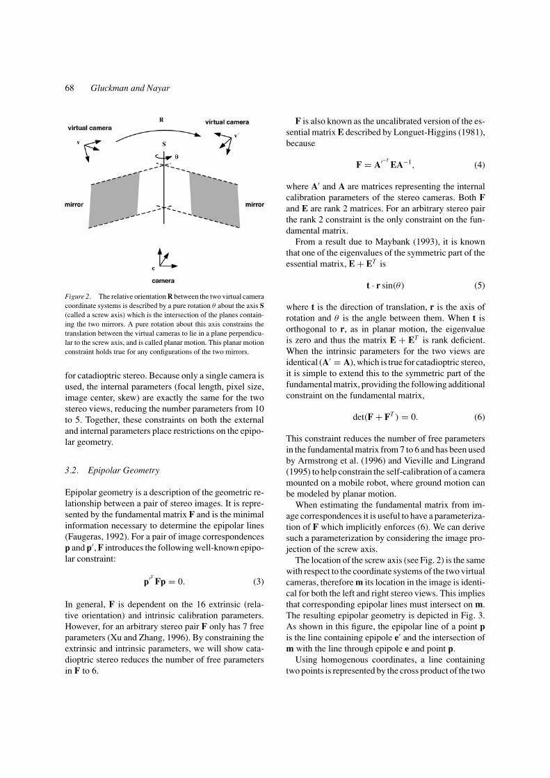
Figure 7. (a) A set of image correspondences used to compute the epipolar geometry. (b) The recovered epipolar geometry. The vertical thickline is m the estimated image of the screw axis, where the corresponding epipolar lines meet. The horizontal thick line is the line connecting thetwo epipoles, the horizon line of the planar motion. The intersection of the two lines is m′ and is used to estimate the focal length.

where

F = [ e′ ]×[ m ]×[ e ]×.

We solve this non-linear minimization problem byusing the Levenberg-Marquardt algorithm (Press etal., 1992). Note that each of e, e′ and m are onlydefined up to a scale factor and therefore need tobe parameterized by two values. This can either bedone with spherical coordinates or by setting a com-ponent to one for each vector. After minimization,Eq. (13) and the estimates of e, e′ and m′ = e ×e′ × m are used to obtain an estimate of the fo-cal length. Figure 7 shows a typical scene with aset of correspondences and the recovered epipolargeometry.

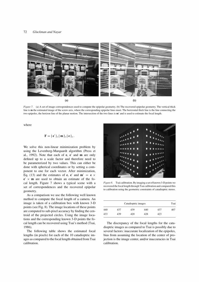
As a comparison we use the following well knownmethod to compute the focal length of a camera. Animage is taken of a calibration box with known 3-Dpoints (see Fig. 8). The image locations of these pointsare computed to sub-pixel accuracy by finding the cen-troid of the projected circles. Using the image loca-tions and the corresponding known 3-D points the fo-cal length can be recovered using Tsai’s method (Tsai,1986).

The following table shows the estimated focallengths (in pixels) for each of the 10 catadioptric im-ages as compared to the focal length obtained from Tsaicalibration.

Figure 8. Tsai calibration. By imaging a set of known 3-D points werecovered the focal length through Tsai calibration and compared thisto calibration using the geometric constraints of catadioptric stereo.

Catadioptric images Tsai

440 437 439 440 437 407

433 439 420 428 423

The discrepancy of the focal lengths for the cata-dioptric images as compared to Tsai is possibly due toseveral factors: inaccurate localization of the epipoles,bias from assuming the location of the center of pro-jection is the image center, and/or inaccuracies in Tsaicalibration.


Figure 9. From corresponding points we reconstruct these squares and measure how close the angles of the four corners are to 90 degrees. (a)In this image the two squares are at an angle. (b) The second image is of a frontal square.

4.2. Euclidean Reconstruction

In the second set of experiments, we determine thequality of calibration by measuring the angles of re-constructed squares. If the estimated focal length isinaccurate then the 3-D reconstruction will have pro-jective distortion causing angles to deviate from 90degrees.

First we estimate the fundamental matrix and thefocal length of the catadioptric stereo system using themethods just described in the previous section. Usingthe focal length, the fundamental matrix and the methodof Longuet-Higgins (1981) we are able to determine therotation and translation up to a scale factor between thetwo virtual cameras.

Then, as shown in Fig. 9 we took images of squaresin several different positions. Using 4 manually se-lected stereo correspondences for each square we re-constructed the square in 3-D and measured the anglesat each corner (which should be 90 degrees). The re-construction was performed by triangulation, using theestimated focal length and extrinsic parameters. The es-timated 3-D point was taken to be the midpoint of theshortest distance between the two back projected rays.Although the direction of translation is only knownup to a scale factor this does not affect the measuredangles.

For the first image a total of 8 angles were measuredfrom the two squares and 4 angles were measured fromthe third square in the second image (see Fig. 9). Thefollowing table contains the computed angles. For eachsquare the angles are measured clockwise from the up-per left corner.

Square 1 89.8 89.2 89.3 91.7

Square 2 91.1 91.4 87.8 89.7

Square 3 90.2 90.4 90.6 88.9

For the 12 angles measured the mean was 90◦ withstandard deviation 1.08◦. Given that we only have pixelresolution for the correspondences this is about as goodas we can expect. Although the first experiment re-vealed that self calibrating the focal length from thecatadioptric geometry is not as accurate as Tsai calibra-tion, it is suitable for quality Euclidean reconstructions.

4.3. Simulations

When self calibrating, there are many factors that mayeffect the estimation of the focal length. In this sectionwe examine the effect of noise, rotation between thevirtual cameras, field of view and location of the imageof the screw axis via simulations. For each simulationwe use an image of size 640×480 pixels and 100 imagecorrespondences. The epipolar geometry is determinedfrom the location of the epipoles and the image of thescrew axis. In this simulation, the optical axis of thecamera is restricted to lie in the same plane as the mir-ror normals. Therefore, the image of the screw axis isvertical and the epipoles lie on a horizontal line throughthe center of the image. The location of the screw axisin the image is described by the parameter c, which isthe distance from the center of the image. The locationof one epipole is determined from the angle of rota-tion θ which is twice the angle between the mirrors.


The other epipole is determined from the focal lengthf . Once the epipolar geometry is determined, imagecorrespondences are generated by randomly selectinga pixel in the left half of the image and then randomlyselecting a corresponding pixel along the epipolar linein the right half of the image. If the pair of image corre-spondences projects to a scene point that does not lie infront of the cameras, the pair is discarded and anotherpair is generated. Once the image correspondences aregenerated, Gaussian noise with standard deviation η isadded to their locations in the image.

For each simulation an estimate f̂ of the focal lengthis obtained from the randomly generated image corre-spondences using the method described in Section 12.Each simulation is performed 100 times and the meansquare error (MSE) (

∑( f̂ − f )2

100 ) is computed. Table 1shows the results of the simulations while varying thelocation of the screw axis c, the amount of noise η,the amount of rotation θ and the field of view as givenby the focal length f . As expected, Table 1(a) showshow the MSE increases as the image of the screw axisapproaches the center of the image c = 0. Table 1(b)shows the response of the MSE to increasing amountsof noise. As shown in (c) the MSE appears to not be

Table 1. The table shows the results from simulations of estimatingthe focal length from a set of randomly generated image correspon-dences. The effect of the following four parameters is examined: thelocation of the screw axis c, the amount of noise η, rotation betweenthe virtual cameras θ , and field of view as determined by the focallength f . For each simulation one parameter is varied while the otherthree remain constant and the mean square error of the estimated fo-cal length is shown. The value for c is the distance in pixels from thecenter of the image. η is the standard deviation of the noise in pixels.θ is the angle of rotation between the virtual cameras and is twicethe angle between the two mirrors.

(a) Constant parameter values: f = 457, η = 0.4, θ = 10◦

Screw Axis (c) 300 270 240 210 180 150 120 90 60 30

MSE of f̂ 1.5 1.8 0.9 1.4 2.0 2.3 3.2 5.7 15.5 130.6

(b) Constant parameter values: f = 457, c = 270, θ = 10◦

Noise (η) 0.0 0.4 0.8 1.2 1.6

MSE of f̂ 0.0 1.8 5.3 13.4 22.0

(c) Constant parameter values: f = 457, c = 270, η = 0.4

Rotation (θ ) 2◦ 6◦ 10◦ 14◦ 18◦

MSE of f̂ 1.5 1.6 1.4 1.1 1.3

(d) Constant parameter values: c = 270, η = 0.4, θ = 10◦

Focal length ( f ) 300 500 700 900 1100

MSE of f̂ 1.8 1.6 8.8 35.1 99.2

effected by the angle between the mirrors. For largefocal lengths and thus small fields of view the MSEincreases as shown in (d).

5. Real-Time Implementation

Real-time stereo systems have been implemented byseveral researchers (Faugeras et al., 1993; Matthies,1993; Kanade et al., 1996; Konolige, 1997). All ofthese systems use two or more cameras to acquire stereodata. Here, we describe a real-time catadioptric stereosystem which uses a single camera and only a PC tocompute depth-maps in real-time. Catadioptric stereois well suited for real-time implementation on a PC be-cause only a single camera and digitizer is needed. Useof a single camera obviates the need for synchroniza-tion hardware and software.

5.1. Sensor Design

Figure 10 shows a picture of two catadioptric stereosensors we have designed. Both designs provideadjustments which allow the rotation and baseline be-tween the two virtual cameras to be controlled. Theschematic in Fig. 11 depicts the catadioptric stereo sen-sor adjustments. When the physical camera is movedaway from the mirrors the two virtual cameras movealong lines normal to the two mirrors, effectively in-creasing the stereo baseline while holding the rotationbetween the cameras constant. In addition, the anglebetween the mirrors can be adjusted. Increasing thisangle results in a larger rotation and baseline betweenthe virtual cameras.

5.2. Calibration and Rectification

To achieve real-time performance it is necessary to havescanline correspondence between stereo views. Thisallows stereo matching algorithms to be implementedefficiently as described by Faugeras et al. (1993). Be-cause catadioptric stereo requires rotated mirrors (ifonly two mirrors are used) and hence rotated views,we must rectify the stereo pair at run-time.

To compute the rectification transform we first needto estimate the fundamental matrix. An estimate of thefundamental matrix is found using the method previ-ously described. After computing the fundamental ma-trix, we find rectification transforms for the left andright images, using a method based on that of Hartley


Figure 10. Catadioptric stereo sensors. (left) A single Sony XC-77 b/w camera and a 12.5 mm Computar lens is used with two high qualityfront silvered Melles Griot 5′′ mirrors. The distance between the camera and mirrors can be altered, which changes the baseline of the stereosystem. The angle between the mirrors can also be adjusted to control vergence and rotation between the stereo views. (right) This compact unituses a single Sony XC-75 b/w camera and a 4 mm Computar pinhole lens with 2′′ Melles Griot mirrors.

and Gupta (1993). Once computed, the rectificationtransforms are used to warp each incoming image atrun-time. The brightness value of each pixel in thewarped image is determined by back projecting to theinput image through the rectification transform andbilinearly interpolating among adjacent pixels.

5.3. Stereo Matching

The underlying assumption of all stereo matching al-gorithms is that the two image projections of a smallscene patch are similar. The degree of similarity iscomputed using a variety of measures such as bright-

Figure 11. Schematic of catadioptric stereo sensor adjustments.By adjusting the angle of the two mirrors the rotation and baselinebetween the virtual cameras can be controlled. The baseline can alsobe altered by adjusting the distance of the physical camera to themirrors.

ness, texture, color, edge orientation, etc. To minimizecomputations, most real-time systems use a measureof similarity based on image brightness. However, dif-ferences in focal settings, lens blur and gain controlbetween the two cameras results in the two patcheshaving different intensities. For this reason many meth-ods, such as normalized cross-correlation, Laplacian ofGaussian, and normalized sum of squared differences,have been employed to compensate for camera differ-ences (Faugeras et al., 1993; Matthies, 1993; Kanadeet al., 1996; Konolige, 1997). By using a single camera,catadioptric stereo avoids both the computational costand loss of information which results from using thesemethods.

As Fig. 12 shows, normalized cross-correlation andthe Laplacian of Gaussian can degrade the performanceof stereo matching due to loss of information andfinite arithmetic. By removing differences in offset andgain, normalized cross-correlation and the Laplacianof Gaussian also remove absolute intensity informa-tion which is useful for matching when only a singlecamera is used.

Each depth map in Fig. 12 was computed using adifferent measure of similarity. The first measure wassum of absolute difference (SAD), the second mea-sure was normalized cross-correlation (NCORR) andthe third was SAD after application of a Laplacian ofGaussian (LOG) operator.3 Due to the loss of infor-mation from the LOG operator, the third measure per-formed the worst. NCORR and SAD performed similarfor large window sizes, greater than 8 × 8. However,for small windows the results from SAD were betterthan NCORR. This is in contrast to two camera stereo


Figure 12. Comparison of three commonly used measures of similarity on an image taken by a catadioptric stereo sensor. (a) Depth mapcomputed using sum of absolute differences. (b) Depth map computed using normalized cross-correlation. (c) Depth map computed using sumof absolute differences after a Laplacian of Gaussian operator was applied. For all three measures a 5 × 5 window was used and no thresholdswere applied.

where NCORR tends to out perform SAD (Faugeraset al., 1993). From a computational standpoint, SADis far more desirable than NCORR, in fact an approx-imation to NCORR was needed to achieve real-timeperformance in Faugeras et al. (1993).

In our implementation, we chose to use SAD as ameasure of similarity for stereo matching. As we have

Figure 13. Stereo image and depth map. On the left is an image taken by a catadioptric stereo system and on the right is the depth map computedwith the SAD measure and a 7 × 7 window.

seen, for single camera stereo SAD has several ad-vantages over other measures: no loss of information,small window sizes can be used and a fast implemen-tation is possible. In addition, SAD keeps the data sizesmall, as opposed to SSD, and is easily implementedon SIMD (single instruction multiple data) processorssuch as those with MMX technology. Furthermore,


Figure 14. The series of depth maps were generated in real-time from these four catadioptric stereo images.

SAD lends itself to efficient scanline correspondencealgorithms.

Stereo matches are found using a standard windowbased search along scanlines. MMX instructions areused to both compute the SAD and determine the bestmatch. The SAD is computed using MMX parallel

vector instructions. We findthe best match through aparallel “tournament” algorithm. The search is lim-ited to an interval of 32 pixels along the epipolar line(scanline) of a 320 × 240 image. In addition we haveimplemented a left-right checking scheme to prunebad matches. Left-right checking computes a depth


measurement for both a patch in the left image andthe patch in the right image it matches. If the twodepths are different then no depth is output at thatpoint.

By using the SAD measure, scanline correspon-dence, and SIMD instructions we are able to achieve athroughput of approximately 20 frames per second ona 300 Mhz Pentium II machine. An example catadiop-tric stereo image and computed depth map are shownin Fig. 13. Figure 14 shows a sequence of depth mapsgenerated in real-time by our system.

We have examined the geometry of stereo with twoplanar mirrors in an arbitrary configuration and shownthat both the relative orientation and the epipolar ge-ometry are constrained by planar motion. In addition,we have shown how the focal length can be extractedfrom a single catadioptric image and demonstrated thisthrough a set of experiments. We have also imple-mented a real-time stereo system which demonstratesthat high quality depth maps can be obtained when asingle camera is used.

In conclusion, we feel that the sensor used to acquirethe stereo data is just as important as the algorithm usedfor matching. In this respect, catadioptric stereo offersa significant benefit by improving the quality of thestereo data at no additional computational cost.

Acknowledgments

This work was supported in part by DARPA’s VSAMImage Understanding Program, under ONR contractN00014-97-1-0553. This paper is an extended versionof a paper presented at CVPR ’99 (Gluckman andNayar, 1999).

Notes

1. Comparison to the Kruppa equations was attempted. However,they gave nonsensical results.

2. www.inria.fr/robotvis/personnel/zzhang/zzhang-end.html3. A sum of squared differences measure (SSD) was also used, how-

ever there was no apparent difference.

References

Armstrong, M. 1996. Self-calibration from image sequences. Ph.D.Thesis, University of Oxford.

Armstrong, M., Zisserman, A., and Hartley, R. 1996. Self-calibrationfrom image triplets. In Proceedings of the 1996 European Con-ference on Computer Vision.

Chaen, A., Yamazawa, K., Yokoya, N., and Takemura, H. 1997.Omnidirectional stereo vision using hyperomni vision. TechnicalReport 96-122, IEICE (in Japanese).

Faugeras, O. 1992. What can be seen in three dimensions with anuncalibrated stereo rig? In Proceedings of the 1992 European Con-ference on Computer Vision. Springer-Verlag: Berlin pp. 563–578.

Faugeras, O. Hotz, B., Mathieu, H., Vieville, T., Zhang, Z., Fau, P.,Theron, E., Moll, L., Berry, G., Vuillemin, J., Bertin, P., and Proy,C. 1993. Real-time correlation-based stereo: Algorithm, imple-mentation and application. Technical Report 2013, INRIA SophiaAntipolis.

Gluckman, J., and Nayar, S.K. 1999. Planar catadioptric stereo:Geometry and calibration. In Proceedings of the 1999 Conferenceon Computer Vision and Pattern Recognition.

Gluckman, J., Nayar, S.K., and Thoresz, K.J. 1998. Real-time om-nidirectional and panoramic stereo. In Proceedings of the 1998DARPA Image Understanding Workshop.

Goshtasby A., and Gruver, W.A. 1993. Design of a single-lens stereocamera system. Pattern Recognition, 26(6):923–937.

Hartley, R.I. 1992. Estimation of relative camera positions for uncal-ibrated cameras. In Proceedings of the 1992 European Conferenceon Computer Vision.

Hartley, R.I. 1995. In defense of the 8-point algorithm. In Proceed-ings of the 5th International Conference on Computer Vision,pp. 1064–1070.

Hartley, R.I. and Gupta, R. 1993. Computing matched-epipolar pro-jections. In Proceedings of the 1993 Conference on ComputerVision and Pattern Recognition.

Hecht, E. and Zajac, A. 1974. Optics. Addison-Wesley: Reading,MA.

Inaba, M., Hara, T. and Inoue, H. 1993. A stereo viewer basedon a single camera with view-control mechanism. In Proceed-ings of the International Conference on Robots and Systems.July1993.

Kanade, T., Yoshida, A., Oda, K., Kano, H., and Tanaka, M. 1996.A stereo machine for video-rate dense depth mapping and its newapplications. In Proceedings of the 1996 Conference on ComputerVision and Pattern Recognition.1996.

Kawanishi, T., Yamazawa, K., Iwasa, H., Takemura, H. and Yokoya,N. 1998. Generation of high-resolution stereo panoramic im-ages by omnidirectional imaging sensor using hexagonal pyrami-dal mirrors. In International Conference on Pattern Recognition1998.

Konolige, K. 1997. Small vision systems: Hardware and implementa-tion. In 8th Int’l Symposium of Robotics Research, Hayama, Japan,Oct. 1997

Longuet-Higgins, H.C. 1981. A computer algorithm for reconstruct-ing a scene from two projections. Nature, 293:133–135.

Mathieu, H. and Devernay, F. 1995. Systeme de miroirs pour lastereoscopie. Technical Report 0172, INRIA Sophia-Antipolis (inFrench).

Matthies, L. 1993. Stereo vision for planetary rovers: Stochastic mod-eling to near realtime implementation. International Journal ofComputer Vision, 8(1):71–91.

Maybank, S.J. 1993. Theory of Reconstruction From Image Motion.Springer-Verlag: Berlin.

Mitsumoto, H., Tamura, S., Okazaki, K., Kajimi, N., and Fukui, Y.1992. 3d reconstruction using mirror images based on a plane sym-metry recovery method. IEEE Transactions on Pattern Analysisand Machine Intelligence, 14(9):941–945.


Murray, D.W. 1995. Recovering range using virtual multicam-era stereo. Computer Vision and Image Understanding, 61(2):285–291.

Nayar, S.K. 1988. Robotic vision system. United States Patent4,893,183.

Nayar, S.K. and Baker, S. 1997. Catadioptric image formation. InProceedings of the 1997 DARPA Image Understanding Workshop,May 1997.

Nene, S.A. and Nayar, S.K. 1998. Stereo with mirrors. In Proceedingsof the 6th International Conference on Computer Vision, Bombay,India, January 1998. IEEE Computer Society.

Nishimoto Y. and Shirai, Y. 1987. A feature-based stereo model usingsmall disparities. In cvpr87, pp. 192–196.

Press, W., Teukolsky, S., Vetterlling, W., and Flannery, B. 1992.Numerical Recipes in C. Cambridge University Press.

Shashua, A. 1998. Omni-rig sensors: What can be done with anon-rigid vision platform? In Workshop on Applications of Com-puter Vision, 1998.

Southwell, D., Basu, A., Fiala, M., and Reyda, J. 1996. Panoramicstereo. In Proceedings of the Int’l Conference on Pattern Recog-nition, 1996.

Teoh, W. and Zhang, X.D. 1984. An inexpensive stereoscopic

vision system for robots. In Proc. Int’l Conference on Robotics,pp. 186–189.

Triggs, B. 1997. Autocalibration and the absolute quadric. In Pro-ceedings of the 1997 Conference on Computer Vision and PatternRecognition, 1997.

Tsai, R.Y. 1986. An efficient and accurate camera calibration tech-nique for 3d machine vision.

Vieville, T. and Lingrand, D. 1995. Using singular displacements foruncalibrated monocular visual systems. Technical Report 2678,INRIA Sophia-Antipolis.

Xu, G. and Zhang, Z. 1996. Epipolar Geometry in Stereo, Motionand Object Recognition. Kluwer: Dordrecht.

Zeller, C. and Faugeras, O. 1996. Camera self-calibration from videosequences: The kruppa equations revisited. Technical Report 2793,INRIA, Sophia-Antipolis, France.

Zhang, Z., Deriche, R., Faugeras, O., and Luong, Q.T. 1995. A ro-bust technique for matching two uncalibrated images through therecovery of the unknown epipolar geometry. Artificial IntelligenceJournal, 78:

Zhang, Z.Y. and Tsui, H.T. 1998. 3d reconstruction from a singleview of an object and its image in a plane mirror. In InternationalConference on Pattern Recognition, 1998.

Documents

Catadioptric Stereo Using Planar Mirrors - … Stereo Using Planar Mirrors 67 Figure 1. Stereo image formation with a single camera and two planar mirrors. A scene point P reﬂected