Fifth International Symposium on Marine Propulsorssmp’17, Espoo, Finland, June 2017

Case Study for the Determination of Propeller Emitted Noise byExperimental and Computational Methods

Lutz Kleinsorge1, Sven Schemmink1, Rhena Klose2, Lars Greitsch1

1Mecklenburger Metallguss (MMG), Waren, Germany2Schiffbau Versuchsanstalt Potsdam (SVA), Potsdam, Germany

ABSTRACT

This paper shows the practical application of differentmethods to determine propeller noise during the designstage by experiments and computational methods.

Different aspects in the determination of propeller noisecharacteristics by model tests are shown. Therefore, cav-itation tunnel tests are performed for different operatingconditions of a propeller mounted behind a container vesseldummy model. The influence of changes in the hydrophonearrangement and the water properties are investigated. Spe-cial focus is given to the extrapolation of the experimentalresults to full-scale.

Besides of model tests numerical propulsion simulationswith different CFD-codes are performed. The radiated pro-peller noise is thereby determined by the Ffowcs-Williams-and-Hawkings-Method. The computational setup is shown.Convergence studies are carried out, varying meshing andnumerical parameters in order to check their influence onthe acoustics. The numerical results are analysed, com-pared, discussed and extrapolated to full-scale propellercondition.

Full-scale measurements of a container vessel were carriedout for validation. The results of cavitation tunnel tests andnumerical simulations are finally compared with these full-scale measurements.

Keywords

Noise, cavitation tunnel experiments, full-scale experi-ments, CFD, Ffowcs-Williams-and-Hawkings-Method.

1 INTRODUCTION

The level of emitted underwater noise is strongly focusedby international organisations and governments due to therising demand of sea transportation and its impact to ma-rine life (McCarthy (2001), Scott (2004)). Thus a broad-band background noise between 100Hz and 300Hz isdominating oceans in northern hemisphere. This back-ground noise is assumed to be the far-field ”‘acousticwaste”’ of merchant ships. As the propeller is consideredto be one of the major sources for underwater noise of mer-chant ships, the precise determination of frequencies andsound pressure levels becomes highly important. Conse-quently, propeller designs have to be evaluated accordingto their noise impact. A leading aspect of marine propeller

noise emission is cavitational behaviour, as it is signifi-cantly affecting (pressure) fluctuations in the flow.

In the past, underwater noise was mainly related to navy,research or fishing aspects. For merchant vessels it wasonly considered when dealing with propeller singing or thecomfort of the crew or passengers. For cruise, researchand fishing vessels, there are minimum noise criteria de-fined by the classification societies, who classify them asa ”silent” ship (e.g. see DNV, 2010). The noise limitingcriteria in these rules are defined by a limiting curve over afrequency range which shall not be exceeded by the emittedsound pressure level (SPL). Usually the SPL is then mea-sured in full-scale by a fixed procedure where the ship ispassing a hydrophone with a defined speed. Obviously thisprocedure is perfect for trial testing, but cannot be used toevaluate the propeller noise during the design. Hence cav-itation test procedures and numerical methods have to bedeveloped in order to evaluate the radiated propeller noisedirectly during the design. Thus a design towards a lessnoisy propeller is possible.

In this paper, different experimental setups and two differ-ent CFD approaches are used to determine the SPL of thepropeller of a container vessel (CV).

2 PROCEDURE FOR ANALYSIS AND SCALING OFNOISE

All recorded noise data in this paper are analysed accord-ing to the ITTC recommended procedures on model scalenoise measurements (ITTC, 2014). Therein noise is ref-erenced as the time varying pressure at a location, usuallygiven as the root mean square:

prms =

√1

T

∫ T/2

−T/2p(t)2 dt (1)

The sound pressure level as quantity of noise is described aslogarithmic ratio of prms and a reference pressure pref =1µPa:

Lp = 10 log10

(p2rmsp2ref

)[dB] (2)

Moreover the time domain signal is transformed into fre-quency domain using a Fourier Transformation in order toevaluate the SPL at certain frequencies. Additionally a fil-ter can be applied to the stochastical narrow band noise tosimplify comparisons. In this paper the 1/3-octave filter is

used, in which the bandwidth is equal to 23 % of the centrefrequency.

Furthermore background noise (from the running facility ortest setup) has to be eliminated from the sound spectrum.Therefore additional noise measurements have to be per-formed by replacing the propeller with a dummy hub. Thecorrection is based on the differences between both SPLs.If the difference is greater than 10 dB no correction has tobe performed, because the propeller noise dominates. If itis smaller than 3 dB the background noise dominates theactual measurement and cannot be used. In between thefollowing expression is used for corrections:

L′p(f) = 10 log10

[10(Lp(f)/10) − 10(LBN (f)/10)

](3)

where LBN is the SPL of the background noise measure-ment.

Additionally wall reflections due to the limited dimen-sions of the test section have to be eliminated. Thereforean acoustic calibration in a free-field environment is per-formed with a known sound source. The noise measured inthe free-field and in the cavitation tunnel are compared anda transfer function is derived by:

Lp,trans(f) = Lp,ff (f) − Lp,ct(f) (4)

where the Index ff refers for the free-field and the indexct to the cavitation tunnel SPL. The transfer function is ap-plied to the L′p:

L′′p(f) = L′p(f) + Lp,trans(f) (5)

Noise levels are influenced by the distance between the ob-server and the source of noise. Therefore a distance nor-malisation is additionally applied for far-field noise. TheLp is corrected by the distance between noise source andobserver d and a reference value, usually dref = 1m, withthe following expression for spherical propagation (unre-stricted, without boundaries):

L′′p,Sphere(f) = L′′p(f) + 20 log10

[d

dref

](6)

For cylindrical propagation, which is applied for the cavita-tion tunnel or other volumes of restricted propagation, thedistance normalisation is done by:

L′′p,Cyl(f) = L′′p(f) + 10 log10

[d

dref

](7)

The noise emitted by the model has to be finally scaled tofull-scale. The ITTC gives the following recommendationfor the scaling of the L′′p :

Ls(f) = L′′p(f) + 20 log10 (corr) (8)

with

corr =

(DS

DM

)z (rMrS

)x(σSσM

)y/2·(nSDS

nMDM

)y (ρSρM

)y/2 (9)

The exponents depend on the test setup and are proposed asx = 1, y = 1 . . . 2 and z = 1 . . . 1.5, see ITTC (1987). Ad-ditionally the frequency has to be shifted in order to correctthe different rates of revolutions of propeller n and cavita-tion numbers σ between model and full-scale:

fSfM

=nSnM

√σSσM

(10)

When comparing with 1Hz spectra, the noise has to be fi-nally retransformed into equivalent 1Hz bandwidth usingthe following expression:

Ls,1Hz(f) = Ls(f) − 10 log10 (0.23f0) (11)

3 CASE STUDY

As case study for the measurement and calculation of pro-peller borne noise a fixed pitch MMG Propeller was cho-sen. The propeller is designed for a 3600TEU containervessel. Main data for both, propeller and ship, are given inTable 1.

Table 1: Main data of propeller and ship

Propeller

Diameter D [m] 7.75Pitch ratio P/D 0.97Area ratio AE/AR 0.73Skew Θ [] 37.9Blades z 5

3600 TEU Container Vessel

Length between perpendiculars LPP [m] 223.60Breadth B [m] 32.20Design draught TD [m] 10.50Draught for noise measurement T [m] 11.52

Figure 1: Arrangement of full-scale measurements

For validation purposes full-scale noise measurements havebeen performed by DW-ShipConsult in the English Chan-nel in 2016 (Schuster, 2016). The noise of the propeller wasmeasured with a hydrophone that was positioned next to a

measuring assistance boat in a defined distance to the pass-ing container vessel. During the noise measurement thenumber of propeller revolutions, speed over ground, windspeed, seastate and current were logged. A sketch of thetest arrangement is shown in Figure 1. Table 2 gives a sum-mary of the operating condition (OP) of the vessel duringthe measurement.

Table 2: Operating condition during full-scale measure-ments (FS)

Parameter FS

Propeller revolutions [rpm] 75Speed over ground [kn] 17.2Speed through water [kn] 14.9Current [kn] 2.3Brake Power [kW] 11960Water depths [m] 64

The measured noise is corrected by elimination of reflec-tions of the sea ground and the free surface. The physicalbehaviour of the ground and the free-surface was also takeninto account in this correction. Since the container vesselwas passing the hydrophone, the recorded time domain sig-nal was divided into three parts before transforming it tofrequency domain. One part covers the arriving of the ves-sel, one the passing and one the departing of the CV. Theresults as given by DW-ShipConsult are shown in Figure 2.As can be seen the difference between them is rather small.In the following sections results of experiments and CFDare compared to the full-scale noise of the passing ship.

120

130

140

150

160

170

180

190

50 50010 100

LP

[dB

re1µPa,1m

]

Frequency [Hz]

arrivingpassingdeparting

Figure 2: Measured sound pressure levels for a containervessel

4 CAVITATION TUNNEL MEASUREMENT

4.1 Test Arrangement

The measured full-scale noise is used as validation data forevaluation of cavitation tunnel tests at SVA.

The OP of the full-scale measurement does not correspondto the results of propulsion tests and trials. Therefore itis assumed that the rpm of the propeller is the most accu-

rately measured parameter during full-scale measurements.Hence the speed and power of the vessel are correctedfor the experiments according to propulsion tests. In Ta-ble 3 the propulsion condition for cavitation tunnel testsand CFD simulation are given. In model tests and RANS-simulations a scaling factor of λ = 31 is used, whereasBEM-simulations are done in full-scale.

Table 3: Corrected operating condition for experiments(EXP)

Parameter EXP

Propeller revolutions [rpm] 75Speed [kn] 17.2Delivered Power [kW] 10560Thrust coefficient 0.1851Cavitation number 3.83

The cavitation observation and narrow band noise measure-ments are performed in the large test section of SVA’s cav-itation tunnel. A dummy model was used together withadditional wake screens in order to reproduce the nomi-nal wake field of the full scale ship, see Heinke (2003) formore information on the procedure. The arrangement ofpropeller and rudder is similar to the full-scale ship. ITTC(2014) recommend different arrangements of hydrophonesfor noise measurements. In total four hydrophones areplaced on the test arrangement to measure the noise:

• hy1 is mounted on the dummy model directly abovethe propeller,

• hy2 is arranged in a decoupled water box,• hy3 is arranged along the direction of flow• and hy4 is arranged transversely to direction of flow.

Figure 3: Test setup and hydrophone arrangement for noisemeasurements

Figure 3 shows a sketch of the overall test arrangement.The cavitation test is run under cavitation number andthrust coefficient identity. The noise measurements havebeen additionally performed at two different levels of oxy-gen content (α/αS = 40% and 60%) in the cavitation tun-nel.

4.2 Results

The measured noise is scaled according to the procedurebriefly explained in section 2. The narrow band data is

transformed to 1/3-octave band. Additionally the noise isfiltered regarding background noise and limited dimensionsof cavitation tunnel, following formula (3) and (4).

4.2.1 Spherical Distance Normalisation

The spherical distance normalisation is the recommendedprocedure by the ITTC for noise measurements (ITTC,2014), as given in formula (6). Furthermore for the scal-ing of SPL and frequency the formula (8) and (10) areused. The exponents of correction terms in (9) are cho-sen as x = 1, y = 2 and z = 1.5. Due to the exponentof y = 2 the tip speed scaling is similar to the methodsof scaling pressure fluctuations. The exponent x is usedfor a distance correction, which was already done by thedistance normalisation. Hence exponent z is used to trig-ger the geometric scaling towards the full-scale noise. Atthe end the 1/3-octave band is retransformed to equivalent1Hz band for a better comparison to the results with thenarrow band full-scale noise results.

Figure 4 shows the scaled noise measured with all four hy-drophones compared with the full-scale measurement inthe English Channel. As can be seen there are large dif-ferences in SPL between the four hydrophones. While hy1(mounted above the propeller) is within the range of thefull-scale measurement, the scaled SPL of hy2 (decoupledwater box) underpredicts the full-scale measurements. Thisalso applies for hy3 and hy4 (arranged in the flow). Therecorded scaled SPL-levels of them are also below the full-scale measurement.

100

120

140

160

180

200

5 50 30010 100

LP

[dB

re1µPa,1m

]

Frequency [Hz]

full-scalehy1hy2hy3hy4

Figure 4: Comparison of full-scale and scaled cavitationtunnel noise measurements as equivalent 1Hz spectra withααS

= 40% oxygen content, spherical distance normalisa-tion

The tests have been performed at an oxygen content ofααS

= 40% and 60% in the cavitation tunnel. The differ-ences between the recorded SPL for both gas contents arerather small. Comparing both tests, the measurements withhigher gas content record a smaller SPL over the frequencyrange, especially when looking on the results of hy2, hy3and hy4 (mounted on the cavitation tunnel wall). Due tothe higher gas content there are more bubbles in the flow.Hence the noise propagation through the water is more dis-turbed. Figure 5 shows the scaled results of hy1 for both

examined gas contents. As can been seen the difference iswithin 3 dB, which is due to the small distance betweenhydrophone and propeller (noise source).

120

130

140

150

160

170

180

190

5 50 30010 100

LP

[dB

re1µPa,1m

]

Frequency [Hz]

full-scalehy1 α/αS = 40%hy1 α/αS = 60%

Figure 5: Comparison of full-scale and scaled cavitationtunnel noise measurements as equivalent 1Hz spectra forhy1, spherical distance normalisation

4.2.2 Cylindrical Distance Normalisation

The spherical distance normalisation is usually applied tonoise measured in a certain distance. Obviously this is notthe case in the restricted environment of a cavitation tunnel.Additionally for using the spherical distance normalisationthe exponents of ITTC scaling have to be triggered in orderto derive an appropriate result. Therefore the analysis arerepeated using a cylindrical distance normalisation as givenin formula (7). Due to the limitations of the cavitation tun-nel dimensions this might be a more suitable approach. Thenormalised SPL is in the following again scaled by formu-lae (8) and (10) to full-scale, but using x = 1, y = 2 andz = 1 as correction exponents (no influence).

120

130

140

150

160

170

180

190

5 50 30010 100

LP

[dB

re1µPa,1m

]

Frequency [Hz]

full-scaleα/αS = 40%α/αS = 60%

Figure 6: Comparison of full-scale and scaled cavitationtunnel noise measurements as equivalent 1Hz spectra forhy1, cylindrical distance normalisation

Figure 6 shows the SPL as equivalent 1Hz band for thehy1. As already shown for the spherical normalisation thescaled results of the cavitation test fits good with the mea-

sured full-scale SPL. Only for frequencies ranging from70 − 120Hz the SPL is overpredicted.

Since the scaled measurements with cylindrical distancenormalisation do not have to be corrected by triggering thenoise scaling exponents x, y and z this procedure is sug-gested to be used when scaling model data to full-scaleSPLs.

4.2.3 Cavitation Phenomena

For the designated propulsion point intermittent tip vor-tex and suction side sheet cavitation in the angle range0 < θ < 60 appears. Intermittent tip vortex cavitationbehind the propeller blade tip has been observed in the an-gle range 70 < θ < 120. Figure 7 shows sketches ofthe cavitation. An angle of θ = 0 refers to the 12 o’clockposition.

Figure 7: Sheet cavitation on propeller at different bladepositions

5 CFD-SIMULATION

Besides the cavitation tunnel test, CFD-simulations are per-formed in order to calculate the propeller radiated noise. Itis essential to be able to evaluate the design according tonoise levels directly in the design process. Therefore twodifferent CFD-approaches to estimate propeller noise emis-sions are shown in the next sections.

5.1 BEM-Simulation

5.1.1 Setup

CFD computations of emitted propeller noise using theBEM-method panMARE are carried out. panMARE isa panel method developed by TUHH (for details see e.g.Berger et al. (2016)). For the simulation the propelleris represented in full-scale. Besides the propeller a flatplate above the propeller simplifying the ship hull is imple-mented. As the wakefield cannot be reproduced preciselywithout taking viscous effects into account, it is consideredvia an external field of velocity derived by model test whichis imported close to the propeller plane (see Figure 8). Thetimestep size is mainly influenced by the stability of cavi-tation simulation and chosen to 2/3 · 10−2 s, which corre-

sponds to a turning angle of θ = 3 per timestep. In totalfive revolutions of the propeller were simulated.

Figure 8: Setup of panMARE simulation

The noise is calculated using the Ffowcs-Williams-and-Hawkings equation according to Gottsche et al. (2017).For recording noise levels, different observers were placedin the simulation domain. They record the noise emittedfrom the solid boundary of the propeller. When cavita-tion occurs, the surface of the cavitation bubble is used.One observer was positioned according to cavitation tun-nel test hy1 in the near-field above the propeller. Additionalobservers were positioned in the far-field along the imag-ined way of the passing hydrophone according to full-scalemeasurements. For the analysis results of the observer po-sitioned perpendicular to ship longitudinal axis are used.This position is comparable to the hydrophone of full-scalemeasurement in closest distance to the passing CV. Thenumber of revolutions of the propeller and the inflow veloc-ity into the computational domain are chosen for the samefull-scale propulsion point as given in Table 3.

5.1.2 Cavitation Phenomena

As basis for noise prediction, precise cavitation simulationis assumed to be crucial because high pressure fluctuationsare caused by cavitation. As cavitation commonly occurson merchant vessels in typical operating conditions, noisesimulations depend on accurate calculation of cavitation ef-fects.

The characteristic of the cavitation behaviour of the sim-ulated propeller is well predicted. The composition anddecomposition of cavitation areas during the blade passagethrough the wake peak is recomputed also in its extents.In Figure 9 the simulated extent of cavitation is comparedwith extent of cavitation measured at SVA cavitation tun-nel. Cavitation computed with BEM method is marked red.The figure is underlain by measured cavitation extents inblack color.

5.1.3 Results

The simulations with BEM-code panMARE were done infull-scale. Hence no scaling has to be applied. Anyhowthe calculated sound pressures have to be transformed tothe 1/3-octave and equivalent 1Hz band. Furthermore adistance normalisation has to be taken into account. Fordifferent points in the simulation domain, different typesof distance normalisation have to be conducted. Accordingto model test normalisation, spherical normalisation is ap-propriate for near-field observers, whereas cylindrical nor-malisation seems to be reasonable for far-field observersin restricted flow regimes. The results of comparison be-tween full-scale measurements, cavitation tunnel measure-ments and BEM-based simulation with spherical normali-sation are shown in Figure 10 and Figure 11.

Figure 9: Comparison panMARE calculated and SVA mea-sured results of cavitation during blade passage

120

130

140

150

160

170

180

190

5 50 30010 100

LP

[dB

re1µPa,1m

]

Frequency [Hz]

full-scale measurementpanMAREpanMARE 1Hz-band

Figure 10: Comparison of full-scale and far-field noiserecorded with panMARE

It can be seen, that the curve progression of sound levelmeasured in full-scale can be reproduced qualitatively wellby BEM calculations. Further the quantitative accordanceof simulation results with full-scale measurements is verysatisfactory as well. Small deviations in sound pressurelevel can be found in the area around 50Hz. In this area ad-

ditional noise sources besides the propeller may have sig-nificant influence on full-scale measurements. Especiallysound peaks in the measurements cannot be recalculated inBEM-simulations. High sound pressure peaks are calcu-lated for the 1st harmonic of blade frequency at 6.25Hzand the 2nd harmonic of blade frequency at 12.5Hz. Forthe far-field simulation the SPL at the 2nd harmonic ofblade frequency is overpredicted by calculation.

Altogether a very good accordance of full-scale mea-surements, cavitation tunnel tests and BEM-simulation isachieved.

120

130

140

150

160

170

180

190

5 50 30010 100

LP

[dB

re1µPa,1m

]

Frequency [Hz]

full-scale measurementcav. tunnel (hy1 )panMAREpanMARE 1Hz-band

Figure 11: Comparison of full-scale and SVA hy1 resultswith near-field noise recorded with panMARE

5.2 RANS-Simulation

Preliminary RANS-calculations are performed in additionto the BEM-simulations.

5.2.1 Setup

For the RANS-Simulation the open-source-code open-FOAM (OF) (OpenCFD, 2017) is used. The propul-sion is performed as a double body simulation neglectingthe free-water-surface. The ship and propeller are simu-lated in model-scale. For recording of noise the Ffowcs-Williams-and-Hawkings-Method was implemented intoOF by Kruger and Kornev (2015). During the simulationan observer recording the propeller noise is placed at thescaled distance of the full-scale measurement (far-field).An additional observer is placed at the same position ashy1 of the cavitation tunnel test. Figure 12 shows the com-putational domain for the CFD simulation, marking alsothe position of the noise observer. Within the implementedMethod, during the simulation run the pressure fluctuationsare logged and finally converted into frequency domain us-ing a Fourier-Transformation.

For the given case study in total three different meshes areused. They consist of tetrahedron cells and vary between2.7 and 12.5 million cells. In all meshes the boundarylayer along the ship-model and the propeller is built withprism-layers, having a non-dimensional wall distance of30 < y+ < 100 next to the wall. For turbulence modelingthe kΩ-SST-model is used. Simulations are performed withthe solver pimpleDyMFoam, neglecting cavitation effects.

The timestep is arranged by keeping the courant numberconstant, which results in a timestep of ≈ 1·10−4 s. There-fore the noise is captured only for six propeller rotations,in order to safe computational efforts. In the simulationthe propeller is rotating with fixed rpm using OFs slidinggrid interface. Figure 13 shows an example of the coarsemesh in the aft part of the ship including the rotating pro-peller domain. The propeller is run at the same thrust as inthe full-scale propulsion point written in Table 3. Conver-gence of propeller thrust and torque is already reached witha medium size mesh of 4.7 million cells. Therefore only re-sults from medium size mesh are shown in the following.

4 LPP 2 LPP

1.5

LPP

Observer far field

Observer near field

flow direction

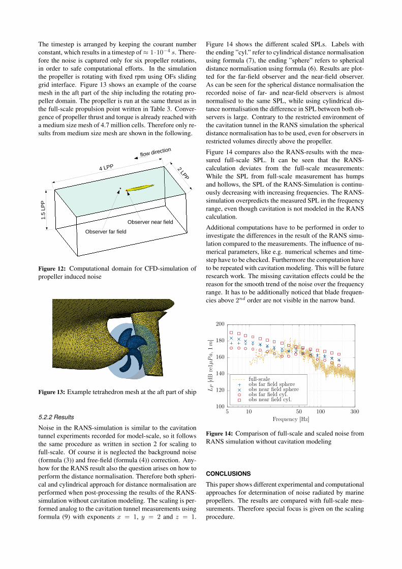
Figure 12: Computational domain for CFD-simulation ofpropeller induced noise

Figure 13: Example tetrahedron mesh at the aft part of ship

5.2.2 Results

Noise in the RANS-simulation is similar to the cavitationtunnel experiments recorded for model-scale, so it followsthe same procedure as written in section 2 for scaling tofull-scale. Of course it is neglected the background noise(formula (3)) and free-field (formula (4)) correction. Any-how for the RANS result also the question arises on how toperform the distance normalisation. Therefore both spheri-cal and cylindrical approach for distance normalisation areperformed when post-processing the results of the RANS-simulation without cavitation modeling. The scaling is per-formed analog to the cavitation tunnel measurements usingformula (9) with exponents x = 1, y = 2 and z = 1.

Figure 14 shows the different scaled SPLs. Labels withthe ending ”cyl.” refer to cylindrical distance normalisationusing formula (7), the ending ”sphere” refers to sphericaldistance normalisation using formula (6). Results are plot-ted for the far-field observer and the near-field observer.As can be seen for the spherical distance normalisation therecorded noise of far- and near-field observers is almostnormalised to the same SPL, while using cylindrical dis-tance normalisation the difference in SPL between both ob-servers is large. Contrary to the restricted environment ofthe cavitation tunnel in the RANS simulation the sphericaldistance normalisation has to be used, even for observers inrestricted volumes directly above the propeller.

Figure 14 compares also the RANS-results with the mea-sured full-scale SPL. It can be seen that the RANS-calculation deviates from the full-scale measurements:While the SPL from full-scale measurement has humpsand hollows, the SPL of the RANS-Simulation is continu-ously decreasing with increasing frequencies. The RANS-simulation overpredicts the measured SPL in the frequencyrange, even though cavitation is not modeled in the RANScalculation.

Additional computations have to be performed in order toinvestigate the differences in the result of the RANS simu-lation compared to the measurements. The influence of nu-merical parameters, like e.g. numerical schemes and time-step have to be checked. Furthermore the computation haveto be repeated with cavitation modeling. This will be futureresearch work. The missing cavitation effects could be thereason for the smooth trend of the noise over the frequencyrange. It has to be additionally noticed that blade frequen-cies above 2nd order are not visible in the narrow band.

100

120

140

160

180

200

5 50 30010 100

LP[dB

re1µPa,1m]

Frequency [Hz]

full-scaleobs far field sphereobs near field sphereobs far field cyl.obs near field cyl.

Figure 14: Comparison of full-scale and scaled noise fromRANS simulation without cavitation modeling

CONCLUSIONS

This paper shows different experimental and computationalapproaches for determination of noise radiated by marinepropellers. The results are compared with full-scale mea-surements. Therefore special focus is given on the scalingprocedure.

Cavitation tunnel tests are performed measuring the noisewith four hydrophones mounted in different positions. Itis shown, that the hydrophone mounted above the pro-peller delivers the best result compared with full-scale mea-surements. The SPL of the full-scale measurement couldbe soundly reproduced by the experimental setup. Hy-drophones mounted on the cavitation tunnel walls directlyin the flow or in a decoupled water box are more effectedby background noise and oxygen content. It has to be con-cluded, that a cylindrical distance normalisation should beused, since no correction with the exponents is necessaryfor scaling.

Two CFD-approaches are performed in order to calculatethe noise emission of the propeller. In both cases theFfowcs-Williams-and-Hawkings-Method is used for noisecalculation.

Preliminary tests for noise propagation with RANS-Methods are performed using OpenFOAM to simulate thepropeller in model-scale without cavitation. It is shown thatfor the RANS-simulation a spherical distance normalisa-tion has to be used before scaling to full-scale. In the sim-ulation differences in SPL to the full-scale measurementoccur. Even though cavitation is not considered the noiseis overpredicted. Therefore the RANS simulation has to befurther improved. Cavitation is to be considered in the fu-ture. Also the numerical schemes and timestep dependencyhas to be investigated more deeply. This will be realized infurther research activities.

The BEM-Solver panMARE simulates the propeller infull-scale with cavitation. Thereby the cavitation phenom-ena is similar to the cavitation tunnel tests. Furthermore itis shown, that the measurements are well reproduced us-ing a spherical distance normalisation for a far-field as wellas for a near-field observer. The BEM-Solver is neglectingreflections of noise by the rudder and hull. The effect of ap-pendages on the emitted noise has to be further evaluated.

To summarize the full-scale measured noise of a containervessel could be soundly reproduced experimentally by cav-itation tunnel tests and numerically by using the BEM-solver panMARE.

ACKNOWLEDGEMENT

This work was funded by the German Federal Ministryof Economic Affairs and Energy (BMWi) based on a de-cision of the German Bundestag, grand No. 03SX377Dand 03SX398B. We also thank DW-Shipconsult for theirsupport with the full-scale measurements and the Univer-

sity of Rostock for the courtesy of the OpenFOAM Ffows-Williams-and-Hawkings implementation. Furthermore wethank the Technical University of Hamburg for the courtesyof providing the panMARE BEM-code.

REFERENCES

Berger, S., Gosda, R., Scharf, M., Klose, R., Greitsch,L. and Abdel-Maksoud, M. (2016), Efficient Numer-ical Investigation of Propeller Cavitation Phenomenacausing Higher-Order Hull Pressure Fluctuations, in‘31st Symposium on Naval Hydrodynamics’, Mon-terey, United States of America.

DNV (2010), ‘Rules for classification of ships: Silent ClassNotation. Part 6. Chapter 24’.

Gottsche, U., Scharf, M., Berger, S. and Abdel-Maksoud,M. (2017), A Hybrid Numerical Method for Investigat-ing Underwater Sound Propagation of Cavitating Pro-pellers, in ‘Proceedings of Fifth International Sympo-sium on Marine Propulsors (SMP)’, Espoo, Finland.

Heinke, H.-J. (2003), The influence of test parameters andwake field simulation on the cavitation and the propellerinduced pressure fluctuations, in ‘STG-Sprechtag Kav-itation’, Schiffbautechnische Gesellschaft.

ITTC (1987), Report of the Cavitation Committee, in‘Proceedings of International Towing Tank Conference1987 (ITTC 87)’, Vol. I, Kobe, Japan, p. 61.

ITTC (2014), ‘Recommended procedure and guidelines:Model scale noise measurements (7.5–02–01–05)’.

Kruger, C. and Kornev, N. (2015), Implementation ofthe Ffowcs Williams–Hawkings Equations into Open-FOAM for Hydro–Acoustic Ship Evaluation, in ‘Pro-ceedings of 18th Numerical Towing Tank Symposium(NuTTS)’, Cortona, Italy, pp. 113–118.

McCarthy, E. M. (2001), International Regulation ofTransboundary Pollutants: The Emerging Challenge ofOcean Noise, in ‘Ocean and Coastal Law Journal, Vol-ume 6:257’.

OpenCFD (2017), ‘OpenFOAM – The open source CFDtoolbox.’.URL: http://www.openfoam.com

Schuster, M. (2016), ‘Unterwasser Schallmessungen, Re-port 1–1073–1’, DW–shipConsult, unpublished, in ger-man.

Scott, K. N. (2004), International Regulation of UnderseaNoise, in ‘ICLQ, Volume 53, S. 287-323’.