Case study: clothes dryer

1

Case study: clothes dryer


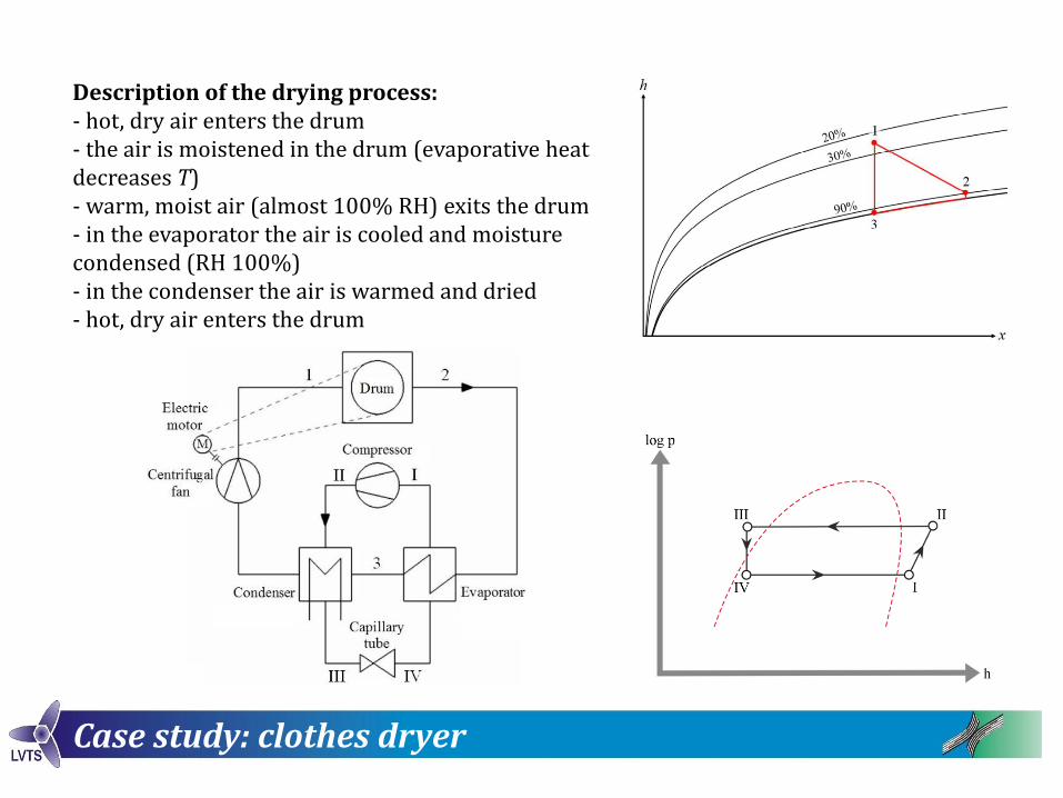
- for drying clothes- machine components: drum (a), filter, door, heat pump (evaporator (d), then condenser (s)), fan with electric motor (b), again drum (a)- drum and fan are driven by the same electric motor

- a description of the process air circuits- a description of the heat pump coolant circuit

2


Description of the drying process:- hot, dry air enters the drum- the air is moistened in the drum (evaporative heat decreases T)- warm, moist air (almost 100% RH) exits the drum - in the evaporator the air is cooled and moisture condensed (RH 100%)- in the condenser the air is warmed and dried- hot, dry air enters the drum

3


Measurements, the following variables are measured:- humidity before and after the drum- temperatures before and after the drum- refrigerant mass- fan speed- drum speed of the drum- energy consumption- mass of condensate

measurements are made for all combinations, a total of 27 measurements:- fan speed 2400, 2900 and 3400 rpm- rotational speeds of drum 36, 47 and 58 rpm- the amount of laundry in the drum 4, 6 and 8 kg

DOF 33

4


Measurement process:- according to IEC 61121 (Tumble dryers for household use - Methods for measuring performance)- were carried out in a room where the temperature and relative humidity were maintained at a narrow interval- regulated voltage and frequency of the network- standardized program (usually eco-labeled)- standardized laundry- initial relative humidity 𝜇𝑖0= 60 % ± 1 %- initial laundry mass 𝑚𝑖

- same procedure of loosening, folding and inserting the laundry into the machine- inal relative humidity 𝜇𝑓0 = 0 % ± 3 %, if not so - repeat

- loundry final weight 𝑚𝑓

- dry loundry weight (capacity) mc

- electric energy consumption Em

𝐸 =𝐸𝑚 ∙

𝜇𝑖0100 −

𝜇𝑓0100 ∙ 𝑚𝑐

𝑚𝑖 −𝑚𝑓𝑡 =

𝑡𝑚 ∙𝜇𝑖0100 −

𝜇𝑓0100 ∙ 𝑚𝑐

𝑚𝑖 −𝑚𝑓


Results:- model of energy consumption E and drying time t- R2>0.975- nf - rotational speed fan- nd - rotational speed (drum)- mc - laundry mass dry 𝐸 = 175,5 + 0,157𝑛𝑓 − 5,56𝑛𝑑 + 151,4𝑚𝑐

𝑡 = 114,2 − 0,01𝑛𝑓 − 0,84𝑛𝑑 + 16,56𝑚𝑐

𝑦 = 𝛽0 + 𝛽1𝑛𝑓 + 𝛽2𝑛𝑑 + 𝛽3𝑚𝑐 + 𝜀

Case study: advection diffusion equation

Case study: Advection difussion equation- we begin with a continuity equation- this one is in a differential form- the flow j can also be written differently- why divergence flow? (next page)

- previously we considered it in an integral form at the introduction to turbine machinery, we called it the general equation of changing property (insert N = m and n = 1) for the continuity equation

- The advection diffusion equation deals with the concentration of a passive polutant, one that moves with a flow without disturbing the flow

𝜕𝜌

𝜕𝑡+ 𝛻 ∙ Ԧ𝑗 = 𝑅

𝜕𝜌

𝜕𝑡+ 𝛻 ∙ 𝜌 Ԧ𝑣 = 𝑅

𝑑𝑁

𝑑𝑡= ඵ

𝐴

𝑛𝜌 Ԧ𝑣 ∙ 𝑑 Ԧ𝐴 +𝜕𝜌

𝜕𝑡ම

𝑉

𝑛𝜌𝑑𝑉


- why divergence of the flow in the second term?- at a point where the diference is ≠ 0, sources or sinks are shown (Fig.)- where the divergence is 0, flow passes through the surface as much as it exits

𝜕𝜌

𝜕𝑡+ 𝛻 ∙ 𝜌 Ԧ𝑣 = 𝑅


- for an incomprehensible flow, the velocity divergence is zero

- we find this from the continuum equation, if there are no external sources, and suppose 𝜌 = 𝑘𝑜𝑛𝑠𝑡.

the first term = 0; from the other we delete density.

𝛻 ∙ 𝑣 = 0

𝜕𝜌

𝜕𝑡+ 𝛻 ∙ 𝜌 Ԧ𝑣 = 0


- An advection diffusion equation is similar to a continuum equation.c is the concentration

- Advection diffusion (also convective diffusion) equation is a continuous equation for the case when we deal with concentration diffusion and convection (motion with motion, flow velocity) of passive pollutant concentration.- The first two terms on the right can be understood as the divergence of the flow due to diffusion (the first part on the right, the diffusion term) and due to advection / convection (the second to the right, the advection)- the diffusion element has a negative sign in relation to the advective, since the concentration diffusion passes from the higher to the lower concentration- D is the diffusion constant

𝜕𝑐

𝜕𝑡= 𝛻 ∙ 𝐷𝛻𝑐 − 𝛻 ∙ 𝑐 Ԧ𝑣 + R


- Advection diffusion equation - understanding of terms

- the first term on the right: if the concentration of the pollutant at a certain site is high, the pollutant passes with diffusion to a location where its concentration is lower- the second term on the right: eg. sugar is inserted upstream to the water, and the concentration of sugar is measured somewhere downstream. At the measured site, the concentration is first low, then it grows (the convection water conveys a high concentration of sugar past the gauge), and then falls again.

𝜕𝑐

𝜕𝑡= 𝛻 ∙ 𝐷𝛻𝑐 − 𝛻 ∙ 𝑐 Ԧ𝑣 + R


- original

- simplification 1: there are no sources or sinks of passive pollutants

- simplification 2: the diffusion constant D is constant, independent of location, direction, and time, so it can be factored out

𝜕𝑐

𝜕𝑡= 𝛻 ∙ 𝐷𝛻𝑐 − 𝛻 ∙ 𝑐 Ԧ𝑣 + R

𝜕𝑐

𝜕𝑡= 𝛻 ∙ 𝐷𝛻𝑐 − 𝛻 ∙ 𝑐 Ԧ𝑣

𝜕𝑐

𝜕𝑡= 𝐷𝛻2𝑐 − 𝛻 ∙ 𝑐 Ԧ𝑣


- Simplification 3: the flow is non-compressible and the velocity divergence = 0

- simplification 4: we are dealing with a stationary phenomenon

- simplification 5: if the velocity is zero, we get Fick's law

𝜕𝑐

𝜕𝑡= 𝐷𝛻2𝑐 − Ԧ𝑣 ∙ 𝛻𝑐

𝛻 ∙ Ԧ𝑣 = 0

𝐷𝛻2𝑐 = Ԧ𝑣 ∙ 𝛻𝑐

Ԧ𝑣 = 0

𝜕𝑐

𝜕𝑡= 𝐷𝛻2𝑐

𝜕𝑐

𝜕𝑡+ 𝛻 ∙ 𝑗 = 0


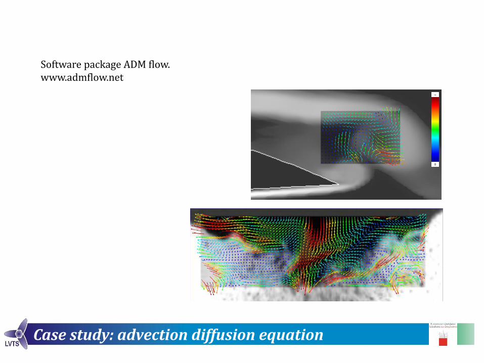
- an example of use for determining the properties of the current around the jellyfish; in the exercises you will consider the flow around the flight wing- jellyfish ... because we do not know geometric shapes, CFD is difficult to perform- we use visualization and advection diffusion equation


In the advection diffusion equation appear (after simplification No. 2):- time derivative of concentration- spatial derivative of concentration- velocity- diffusion constant

If we can measure the concentrations, we can calculate the velocity. If we later use the NS equation, then we can calculate the pressure.

𝜕𝑐

𝜕𝑡= 𝐷 𝛻2𝑐 − 𝛻 ∙ 𝑐 Ԧ𝑣

= 𝐷𝛻2𝑐 − 𝑐 𝛻 ∙ 𝑣 − Ԧ𝑣 ∙ 𝛻𝑐


In the image, we measure the brightness in a single point. For a color RGB camera at each point the sensor measures 3 values, one for each color component RGB (red, green blue), and at the BW camera for each point one gray component, grayness.The gray value of N is between 0 and 255, for the 8 bit CCD camera sensor.Assuming that the light / grayness in the image is proportional to the concentration, visualization can be used to provide us with data for the advective diffusion equationApproximation is valid for low concentrations ...

In the advection diffusion equation we replace

𝜕𝑐

𝜕𝑡= 𝐷 𝛻2𝑐 − 𝛻 ∙ 𝑐 Ԧ𝑣 →

𝜕𝑁

𝜕𝑡= 𝐷 𝛻2𝑁 − 𝛻 ∙ 𝑁 Ԧ𝑣

𝑐 → 𝑁


Now it's not far to the end ...Advection diffusion equation for N is written in cartesian coordinates xi

From the above equation we can calculate all components of the velocity.

𝜕𝑁

𝜕𝑡= 𝐷 𝛻2𝑁 − 𝛻 ∙ 𝑁 Ԧ𝑣

𝜕𝑁

𝜕𝑡= 𝐷 𝛻2𝑁 − 𝑁𝛻 ∙ Ԧ𝑣 − Ԧ𝑣 ∙ 𝛻𝑁

𝜕𝑁

𝜕𝑡= 𝐷

𝜕2𝑁

𝜕𝑥𝑖2 − 𝑁

𝜕𝑣

𝜕𝑥𝑖− 𝑣𝑖

𝜕𝑁

𝜕𝑥𝑖


In the advection diffusion equation, the time derivatives of the concentration appear ...


... and spatial derivatives concentration


Solution: spatial velocity depending on the time for all the images taken. By averaging, we get a solution similar to Reynolds's averaging in CFD.The jellyfish is below on the left.


There are some examples of solvingadvection diffusion equationswith visualization.


Software package ADM flow.www.admflow.net

22

Case study: power model for water height

Case study: Power models, modeling of water level at the confluencethe largest dimensionless wave height 𝑍𝑀𝐶 at the confluence and x coordinate 𝑋𝑀𝐶 (the place in the image marked with an asterisk)

𝑍𝑀𝐶 =𝐻𝑀𝐶ഥ𝐻

= 𝐹𝑟𝑔 ∗ 𝐹𝑟𝑠1,4 ∗

𝑏

ഥ𝐻

(−0,6)

𝑋𝑀𝐶 =𝑥𝑀𝐶𝑏

= 1,1 ∗ cos 𝜃 −4,5 ∗𝐻𝑠𝐻𝑔

(−0,6)

∗ 𝐹𝑟𝑔0,8 ∗ 𝐹𝑟𝑠

0,1 ∗𝑏

ഥ𝐻

(−0,85)

23

Case study: power model for water height

Power regression - an example of modeling the height of water at the confluencemaximum wave height

24

Case study: mass transfer

Case study: Power model, mass transfertransfer of matter from a moving droplet to a stationary liquid: the transmission coefficient depends on the speed of the drop 𝑣, density 𝜌, viscosity 𝜇, diameter 𝑑 and diffusion coeffient 𝐷

the equation can be approximated by

if the constants are 𝑐 non-dimensional, then both elements have to the right the same dimension as k, so we can write down

unit m (length)

unit with (time)

and unit kg (mass)

𝑘 = 𝑓 𝑣, 𝜌, 𝜇, 𝑑, 𝐷

𝑘 = 𝑐1𝑣𝑎𝜌𝑏𝜇𝑐𝑑𝑒𝐷𝑓 + 𝑐2𝑣

𝑔𝜌ℎ𝜇𝑖𝑑𝑗𝐷𝑘

+1 − 𝑎 + 3𝑏 − 𝑐 + 𝑒 − 2𝑓 = 0

−1 + 𝑎 + 𝑒 + 𝑓 = 0

−𝑏 − 𝑒 = 0

25

Case study: mass transfer

Power regression - an example of mass transferif we solve a system of equations, we get it

we can process this in

or

Sh = Sherwood number (convective mass transfer / diffusion)Re = Reynolds number (inertial forces/viscous forces)Sc = Schmidt number (viscous diffusion/molecular diffusion)

𝑘 = 𝑐1𝑣𝑎𝜌𝑎−1+𝑓𝜇1−𝑎−𝑓𝑑𝑎−1𝐷𝑓

𝑘𝑑

𝐷= 𝑐1

𝜌𝑣𝑑

𝜇

𝑎𝜇

𝜌𝐷

1−𝑓

𝑆ℎ = 𝑐1𝑅𝑒𝑎𝑆𝑐1−𝑓

Documents

Case study: clothes dryer