Case Study 3

Ocean-Atmosphere Exchanges of Persistent OrganicPollutants on the Atlantic Ocean

Elena Jurado∗1 Rafael Simó2 and Jordi Dachs3

3.1 Background Information

Persistent Organic Pollutants (POPs), also known as Persistent Bioaccumulable Toxic

chemicals (PBTs), are bioaccumulable compounds of prolonged environmental per-

sistence and are susceptible to long-range atmospheric transport. They have been

detected in all the environmental compartments, even in remote areas such as

the open ocean and the polar regions, where POPs have never been manufactured

or used. Furthermore, once they appear in the environment they do not degrade.

Instead, they recycle and partition between the major environmental media, and

are an environmental concern since their toxic effects do not disappear, and their

control is difficult. Their physicochemical properties, such as the high lipid/organic

solubility, result in their bioaccumulation in lipid-rich tissues and ‘bio-magnification’

through the food chain. Even at low concentrations they are toxic to humans

and wildlife, with suspected effects including carcinogenesis, immune dysfunction,

neurobiological disorders and reproductive and endocrine disruption.

POPs comprise man-made organo-halogenated compounds (e.g. pesticide POPs

such as DDT, industrially produced POPs such as polychlorinated biphenyls (PCBs) or

POPs that are unintended byproducts such as polychlorinated dibenzo-p-dioxins and

polychlorinated dibenzofurans (PCDD/Fs) and other chemicals that can, in part, be

biogenic such as polycyclic aromatic hydrocarbons (PAHs). In particular, man-made

POPs were initially produced and used in the 1940s. During the 1960s and 1970s,

the use of certain POPs in industry or as pesticides increased dramatically. The first

political regulations for the production and use of POPs dates from the late 1970s.

Since then, a number of politically-binding regulations have entered into force to

reduce or eliminate their emissions: the Convention on Long-Range Transboundary

1Institute for Marine and Atmospheric Research Utrecht (IMAU), Utrecht University, Princetonplein5, 3584 CC Utrecht, The Netherlands. ∗Email address: e.juradocojo@uu.nl

2Marine Sciences Institute, CMIMA-CSIC, Passeig Marítim de la Barceloneta 37-49, Barcelona 08003,Spain

3Department of Environmental Chemistry, IIQAB-CSIC, Jordi Girona 18-26, Barcelona 08034, Spain

35

36 • Handbook of Satellite Remote Sensing Image Interpretation: Marine Applications

Air Pollution on POPs, the Stockholm Convention on POPs, and, at the European

Level, the Water Framework Directive.

Despite regulations, they still cycle between the different environmental com-

partments and there are non-controlled sources as well. For example, high con-

centrations of PCBs have been reported in arctic wildlife and breast milk. This

is of special concern, not only because those contaminants were already banned

in the late 1970s, but also because of the distance from the source where those

pollutants were produced. There is thus a global occurrence of these contaminants

and an urgent need to control their levels in the environment. Sampling of POPs,

however, is time-consuming and expensive compared to many other contaminants.

In this context, global models are a valuable tool to predict and understand the

distribution of POPs. Satellite data, with their global synoptic coverage, can provide

environmental input data to global POPs models, as we will see later.

To understand how we can use remote sensing data to model the global dis-

tribution of POPs, we provide here a short explanation of the partitioning of POPs

in the different environmental media. Because both atmosphere and oceans are

critical compartments in the global distribution and cycling of POPs, the analysis

will focus in the ocean-atmosphere exchanges of POPs. Atmospheric emissions and

subsequent long-range transport have proven to provide a mechanism to distribute

POPs widely through the global environment. In fact, atmospheric deposition of

POPs may be the major process by which they impact remote oceans and other

pristine environments. On the other hand, the oceans are also critical in the global

cycling of those pollutants; their large volumes imply that they may represent an

important inventory of POPs.

Figure 3.1 shows a diagram of the major processes affecting the transfer of POPs

between the atmosphere and the ocean. In the atmosphere, POPs partition between

the gas and aerosol phases and they may then be removed by three processes: dry

deposition of aerosol-bound pollutants, diffusive gas exchange between the atmo-

sphere and the ocean, and scavenging by rain (either from gas or particulate phases),

the latter termed wet deposition. In the water column, POPs can be found either dis-

solved or sorbed to particulate organic matter. Dissolved POPs can revolatilize back

to the atmosphere or they can stay in the water column and become bioavailable,

i.e. they can be incorporated into the biota by passive diffusion. POPs sorbed to

particulate organic matter cannot revolatilize back to the atmosphere, but can be

deposited by gravity or sinking. In both particulate and dissolved phases, they are

subject to turbulent mixing throughout the water column. Finally, in each medium,

POPs are subject to degrade, but those fluxes are generally considered negligible. By

means of simplification, no lateral advection of contaminants is considered, which

is an assumption generally accepted in the open ocean, where contaminants enter

primarily via atmospheric deposition.

The processes affecting the transfers of POPs between the atmosphere and the

ocean are evaluated quantitatively by means of fluxes (F [ng m−2 s−1 ]), whose

Ocean-Atmosphere Exchanges of Persistent Organic Pollutants • 37

!"#$"%&'!(

)*++",*-'(

,*'.*'/(

)#0(

)&1-,*!*-'(

atmosphere

23(

2/(

4*#534!&#(

&6274'/&((

21()&/#4)4!*-'(

3&!(

)&1-,*!*-'()&/#4)4!*-'(

dissolved particles

gaseous

24&#(

aerosol

water

Figure 3.1 Major processes affecting the transfer of POPs between the atmo-sphere and the ocean. The amount of contaminant in an environmental mediais denoted by its concentration, C. Fluxes are marked in capital letters.

simplified mathematical formulation is presented next. Advective processes, where

contaminants are transported by means of directed motion, such as dry deposition,

wet deposition and sinking, are governed by:

Fadvective = vC (3.1)

where v [m s−1] is the advective velocity and C [ng m−3] is the concentration of the

chemical.

Diffusive processes, such as air-water exchange or turbulent flux, where contam-

inants are transported by random motion, are governed by Fick’s First Law:

Fdiffusive = −D∂C∂x

(3.2)

where D [m2 s−1] is the molecular diffusivity and ∂C/∂x is the gradient of concentra-

tions in the x direction, along which the change of concentration of the contaminant

occurs. The mathematical formulation of diffusion becomes more complex if the

transport occurs between two media, as would be the case of the diffusive transport

across the air-water interface. The resultant flux is then a combination of molecular

and turbulent diffusion.

The last type of process, the degradation process, produces a loss in the system,

and is characterized by a first order decay rate, kdegr [s−1].

Ftransformation = hkdegrC (3.3)

38 • Handbook of Satellite Remote Sensing Image Interpretation: Marine Applications

where h [m] is the height of the volume where degradation is acting.

It is important to note that the magnitude of the contaminant fluxes is a function

of the measured concentration, physicochemical parameters, and environmental

conditions. The environmental conditions do not only determine the parameters v,

D and kdeg, from Equations 3.1 to 3.3, they also influence the ratio of contaminant

concentrations between two different phases of equilibrium. This ratio is termed

the equilibrium partition coefficient and it is essential in the modelling of POPs.

For example, the gas-particle partition coefficient Kp will allow us to calculate the

concentration of a certain POP in its aerosol phase, knowing its concentration in the

gaseous phase and assuming equilibrium conditions, which is a common assumption

since these compounds are continuously seeking to equilibrate between the different

reservoirs.

This case-study shows an example of the application of satellite data to estimate

the spatial and temporal distribution of atmospheric-ocean fluxes of POPs in the

Atlantic Ocean. It has been developed in detail in various publications (Dachs et al.

2002; Jurado et al. 2004; 2005; 2008) and it is based on the previous work of Dachs

et al. (2002) and Simó and Dachs (2002). Essentially, satellite retrieved parameters

and air measured concentrations (gaseous and aerosol phases) in two north-south

campaigns across the Atlantic (Lohmann et al. 2001; Jaward et al. 2004) have

been coupled in a 0D (i.e. zero- dimensional), spatially resolved, box model. A 0D

model means, for example, that the vertical variation of the fluxes is not accounted

for. A box model means that the system has been subdivided into well-mixed and

interconnected compartments. The model was applied using monthly means of

satellite data and assuming that measured atmospheric concentrations are constant

in time.

Satellite-based environmental data correspond to monthly climatological means

(average 2001 – 2003) of Level 3 data with global coverage and resolutions of 1◦x1◦

or 0.5◦x0.5◦, presented in greater detail below. Level 3 refers to data that is designed

for the end user, which has been calibrated with in situ observations and data

assimilation techniques.

3.2 Satellite Data Used

3.2.1 Wind speed distributions at 10m above the surface of the sea

The surface wind speed was used in this study (u10, m s−1). Values were ob-

tained from the NOAA Special Sensor Microwave/Imager (SSM/I) at a resolution

of 1◦x1◦ and an accuracy of ± 2 m s−1 (http://lwf.ncdc.noaa.gov/oa/satellite/

ssmi/ssmiwind.html).

Ocean-Atmosphere Exchanges of Persistent Organic Pollutants • 39

3.2.2 Aerosol parameters over the oceans

Aerosol values at a resolution of 1◦x1◦ were obtained from the Moderate-Resolution

Imaging Spectrometer Instrument (MODIS, http://modis.gsfc.nasa.gov/) on board

the Terra satellite, part of NASA’s Earth Observing System (EOS). In particular,

we used the effective radius (reff, µm) and its standard deviation (which provides

information about the size distribution of aerosols), the aerosol optical depth

(AOD) and its standard deviation (related to the aerosol density in the atmosphere),

and the fraction of optical depth corresponding to submicron aerosols (η, [0-1]).

The approximate accuracy is ± 0.1µm for reff, ±0.03*AOD (or ±0.05*AOD in dust

regimes), and 25% for η. MODIS aerosol retrieved measurements refer to values

integrated over the air column and they refer to the size range detected by the

instrument (aerosol diameters from 0.1 to 20 µm). This information is important to

derive aerosol dry deposition velocities from satellite data (Jurado et al. 2004).

It should be pointed out that deriving aerosol sizes or concentrations from

remote sensing measurements has a higher uncertainty than other variables such

as wind speed, SST and p0 used in this study. Until recently, MODIS was the only

sensor that gave information about aerosol sizes. This area of research is currently

undergoing rapid development, and several satellite-based light imaging radars

(lidars) are being launched (e.g. CALIPSO from NASA), providing information about

the vertical structure of aerosol plumes, which is not available from MODIS data.

3.2.3 Precipitation data

Values of monthly rainfall rates (p0, [mm month−1]) and the fractional occurrence

of precipitation (f, [0-1]) were obtained from SSM/I NOAA at a resolution of 1◦x1◦

(http://www.ncdc.noaa.gov/oa/satellite/ssmi/ssmiprecip.html). Determination

of rainfall by passive microwave sensors, such as SSM/I, may be underestimated

during low rainfall periods and overestimated during wet periods, leading to some

inaccuracies in the tropics. However, rainfall retrieval over the ocean from SSM/I

represents the best compromise between estimation accuracy and spatial data

coverage. Uncertainty is about 15 to 30% when compared to rain gauge data sets.

A novelty of the use of precipitation data in wet deposition modelling of POPs

has been the consideration of the influence of the frequency of rain (f). The instanta-

neous flux of contaminants scavenged by rain may be substantial in a month with a

low frequency of rain and a high rainfall rate. The methodology developed is further

described in Jurado et al. (2005).

3.2.4 Sea Surface Temperature (SST, [K])

Values were obtained from the Along Track Scanning Radiometer (ATSR) on board

the European Space Agency ERS-2 satellite (http://www.atsr.rl.ac.uk/). SST im-

40 • Handbook of Satellite Remote Sensing Image Interpretation: Marine Applications

ages consist of monthly averaged data with a resolution of 0.5◦x0.5◦ and an accuracy

of ±0.3K.

3.2.5 Chlorophyll-a concentration (chl-a, mg m−3)

This was estimated from reflectance signals obtained from NASA’s Sea-Viewing Wide

Field-of-view Sensor (SeaWiFS) (http://www.csc.noaa.gov/crs/rs_apps/sensors/

seawifs.htm). The resolution is 1◦x1◦ and accuracies are around the 15%. This

data allows the estimation of the phytoplankton biomass distribution in the surface

mixed layer.

3.3 Demonstration Section

In this section we present the values of dry deposition flux, latitudinally-averaged for

the Atlantic, together with satellite global maps of data that have a potential effect

in the magnitude of the flux. Visually-based interrelations between this flux and

that pertaining to the satellite data are explained, so that one can acquire the skills

required to use the satellite images to understand better the latitudinally-averaged

fluxes of POPs.

0 1 2 3 4

90°N

60°N

30°N

0

30°S

60°S

90°S

F DD [pg m -2 d-1]

Cl5DDs Cl7DDs

Dry deposition �ux

Figure 3.2 Averaged latitudinal profile of the dry aerosol deposition fluxes forCl5DDs and Cl7DDs over the Atlantic Ocean, for the period October-December1998.

As a reminder, the dry aerosol deposition flux is the deposition of aerosol-

bound contaminants in the absence of rain. Figure 3.2 depicts an example of

a latitudinally-averaged profile of dry deposition flux over the Atlantic for two

Ocean-Atmosphere Exchanges of Persistent Organic Pollutants • 41

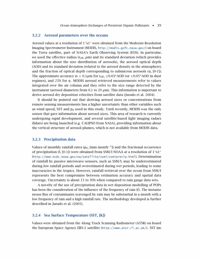
reference compounds, the penta-dibenzo-p-dioxin (Cl5DDs) and the hepta-dibenzo-

p-dioxin (Cl7DDs). The flux has been estimated using the methodology presented in

the previous section, but developed in detail in Jurado et al. (2004). An example of

measured air concentration data is depicted in Figure 3.3.

GAS: CG

[fg m-3]

AEROSOL: CAER

[fg m-3] (Lohmann et al. 2001)

Cl5DDs

Cl5DDs

(Lohmann et al. 2001)

(a) (c)

(b)

RRS Bransfield Oct-Dec 1998. PCDD/Fs.

Lohmann et al. 2001

Figure 3.3 Latitudinal profiles of Cl5DDs measured during a north-southAtlantic cruise: (a) gas and (b) aerosol sorbed profiles. Figure (c) depicts thecruise track.

For the interpretation of Figure 3.2 we provide the following satellite images: sea

surface temperature (SST) (Figure 3.4), indicative of the temperature of the air close

to the water surface, the effective radius (reff) (Figure 3.5), defined as the weighted

integral of the volume-surface ratio and indicative of the size of the aerosol, the

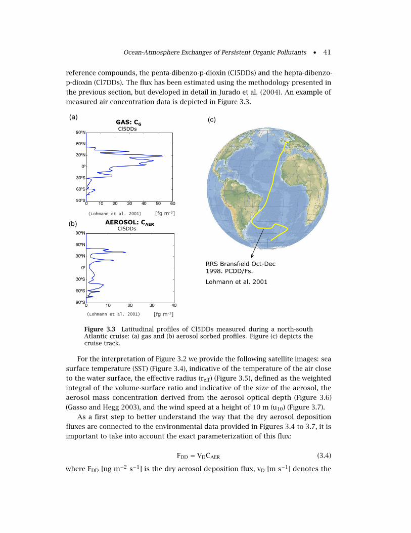
aerosol mass concentration derived from the aerosol optical depth (Figure 3.6)

(Gasso and Hegg 2003), and the wind speed at a height of 10 m (u10) (Figure 3.7).

As a first step to better understand the way that the dry aerosol deposition

fluxes are connected to the environmental data provided in Figures 3.4 to 3.7, it is

important to take into account the exact parameterization of this flux:

FDD = VDCAER (3.4)

where FDD [ng m−2 s−1] is the dry aerosol deposition flux, vD [m s−1] denotes the

42 • Handbook of Satellite Remote Sensing Image Interpretation: Marine Applications

aerosol overall dry deposition velocity and CAER [ng m−3] is the POP aerosol-phase

Figure 3.4 Global distribution of Sea Surface Temperature (SST) in January(climatological monthly mean of 1998 – 2000).

Figure 3.5 Global distribution of effective radius (reff) over the oceans inNovember (climatological monthly mean of 1998 – 2000).

Ocean-Atmosphere Exchanges of Persistent Organic Pollutants • 43

Aerosol mass concentration [µg m-3]

Figure 3.6 Global distribution of the aerosol mass concentration over theoceans in November (climatological monthly mean of 1998 – 2000). Derivedfrom MODIS Aerosol Optical depth parameter, and the algorithm developed inGasso and Hegg (2003).

concentration.

From Equation 3.4 one should note that the dry aerosol deposition flux is directly

proportional to the POP-aerosol-phase. Indeed, major dry deposition fluxes will be

found in regions with major amounts of contaminants in the aerosol phase. The

tendency to be in the aerosol-phase instead of the gas-phase is highly dependent on

the air temperature, so that a lower air temperature will cause a higher partition to

the aerosol phase. A map of SST , representative of the temperature of the air above

the ocean surface, provides information of the regions over the oceans with a higher

proportion of contaminants in the aerosol phase i.e. the temperate regions at higher

latitudes.

The sea surface temperature (Figure 3.4) cannot be the only variable affecting the

latitudinal trend in the fluxes from Figure 3.2, because it follows a smooth increase

towards higher latitudes, while the fluxes depict an important variability. Other

environmental variables, with a higher patchiness, should affect the magnitude of the

fluxes. We envisage that the effective radius (Figure 3.5), aerosol mass concentration

(Figure 3.6) or the wind speed (Figure 3.7) could contribute because their global

distribution presents a higher variability than the SST.

How do Figures 3.5 to 3.7 combine to explain the fluxes in dry deposition of

44 • Handbook of Satellite Remote Sensing Image Interpretation: Marine Applications

] u10 [m s-1

Figure 3.7 Global distribution of the wind speed (u10) over the oceans inNovember (climatological monthly mean of 1998 – 2000).

POPs? The answer is found in the next variable, not yet assessed in equation 3.4,

the overall dry deposition flux vD. The vD is greatly influenced by the aerosol size,

by the atmospheric turbulent diffusion and by the atmospheric growth of particles

at a high humidity. In particular, vD will increase with the particle diameter and the

wind speed for diameters >0.1 µm, governed by gravitational settling. Also, a high

concentration of aerosol in the atmosphere will increase the dry deposition velocity.

Knowing this information, it is possible to relate the large increase in the fluxes

around 15◦S to an increase of the effective radius, indicative of the size of aerosol

particles, or the aerosol mass concentration in the Atlantic around this latitude.

Furthermore, we can relate the peaks in the dry deposition fluxes around 60◦S to

strong winds in the Southern Ocean.

We end this section by explaining the differences in the fluxes of the two depicted

contaminants: Cl5DDs and Cl7DDs. This is an example of how physico-chemical

properties of the chemical compounds affect the fluxes. We see that the relative

increase of dry deposition fluxes of the Cl7DDs in higher latitudes is greater than for

Cl5DDs. This is because Cl7DDs sorb stronger to the organic matter of the aerosol,

causing a major relative presence of those compounds in the aerosol phase. As a

general rule, compounds with higher molecular weight will have less solubility in

water, a higher affinity to organic matter and a lower vapour pressure.

Ocean-Atmosphere Exchanges of Persistent Organic Pollutants • 45

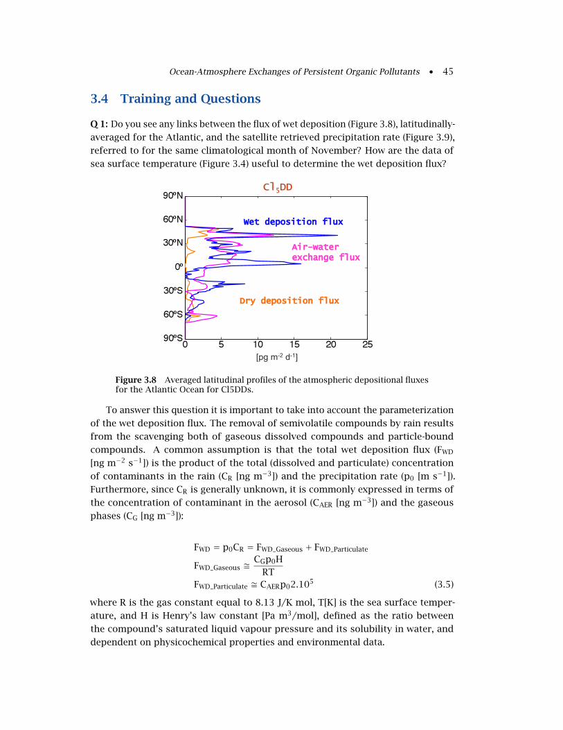
3.4 Training and Questions

Q 1: Do you see any links between the flux of wet deposition (Figure 3.8), latitudinally-

averaged for the Atlantic, and the satellite retrieved precipitation rate (Figure 3.9),

referred to for the same climatological month of November? How are the data of

sea surface temperature (Figure 3.4) useful to determine the wet deposition flux?

Dry deposition flux

Wet deposition flux

Air-water exchange flux

[pg m-2 d-1]

Figure 3.8 Averaged latitudinal profiles of the atmospheric depositional fluxesfor the Atlantic Ocean for Cl5DDs.

To answer this question it is important to take into account the parameterization

of the wet deposition flux. The removal of semivolatile compounds by rain results

from the scavenging both of gaseous dissolved compounds and particle-bound

compounds. A common assumption is that the total wet deposition flux (FWD

[ng m−2 s−1]) is the product of the total (dissolved and particulate) concentration

of contaminants in the rain (CR [ng m−3]) and the precipitation rate (p0 [m s−1]).

Furthermore, since CR is generally unknown, it is commonly expressed in terms of

the concentration of contaminant in the aerosol (CAER [ng m−3]) and the gaseous

phases (CG [ng m−3]):

FWD = p0CR = FWD_Gaseous + FWD_Particulate

FWD_Gaseous �CGp0H

RTFWD_Particulate � CAERp02.105 (3.5)

where R is the gas constant equal to 8.13 J/K mol, T[K] is the sea surface temper-

ature, and H is Henry’s law constant [Pa m3/mol], defined as the ratio between

the compound’s saturated liquid vapour pressure and its solubility in water, and

dependent on physicochemical properties and environmental data.

46 • Handbook of Satellite Remote Sensing Image Interpretation: Marine Applications

Figure 3.9 Global distribution of the precipitation rate (p0) over the oceans inNovember (climatological monthly mean of 1998 – 2000).

Q 2: Which are the main satellite images, already displayed in this case-study,

that potentially affect the flux of air-water exchange? Also consider the global

distribution of chlorophyll-a depicted in Figure 3.10.

Again, to answer this question, it is important to first examine the parameteriza-

tion of this flux. The flux of gaseous contaminants between the atmosphere and the

oceans is driven by a concentration difference and by the transport due to molecular

and turbulent motion. This flux combines turbulent and molecular diffusion since it

occurs through an interface, thus the parameterization is not straightforward. It is

based in the classical two-layer stagnant boundary layer model, where it is assumed

that a well-mixed atmosphere and a well-mixed surface ocean are separated by a

stagnant film through which gas transport is controlled by molecular diffusion. The

resulting net air-water exchange flux (FAW [ng m−2 s−1]) is a function of the air-water

mass transfer coefficient kAW, with velocity units ([m s−1]), the POP dissolved con-

centration in the water (CdisW [ng m−3]) and the corresponding concentration in the

gaseous phase in equilibrium (CG RT/H). This flux is, in fact, the net difference of

two processes acting in parallel: absorption of gaseous POPs from the atmosphere to

the water (FAW_abs) and the volatilization of POPs from the water to the atmosphere

(FAW_vol).

FAW = FAW_abs − FAW_vol = kAW

(CGRT

H− Cdis

W

)(3.6)

where H is, again, the Henry’s law constant and kAW the air-water mass transfer

Ocean-Atmosphere Exchanges of Persistent Organic Pollutants • 47

Figure 3.10 Global distribution of the concentration of chlorophyll-a (chl-a)in the oceans in January (climatological monthly mean of 1998 – 2000).

coefficient. kAW describes the rate at which chemicals partition between air and

water surface and comprises resistance to mass transfer in both water (kW [m s−1])

and air films (kA [m s−1]):

1kAW

= 1kW+ RT

kAH(3.7)

These mass transfer coefficients have been empirically defined based upon field

studies using tracers such as CO2, SF6 and O2. kW is calculated from the mass trans-

fer coefficient of CO2 in the water side (kW,CO2 [m s−1]), itself generally correlated

solely to wind speed (u10, [m s−1]) (Nightingale et al. 2009):

kW = kW,CO2

(ScPOP

600

)−0.5(3.8)

kW,CO2 = 0.24u210 + 0.061u2

10(1/100)(1/3600) (3.9)

where ScPOP [dimensionless] is the Schmidt number of the POP and 600 is the Schmidt

number of CO2 at 298K. Similarly kA can be estimated from the mass transfer

coefficient of H2O in the air side (kA,H2O [m s−1]), also generally parameterized as a

function of the wind speed (Schwarzenbach et al. 2003):

kA = kA,H20

(DPOP,a

DH20,a

)0.61

(3.10)

48 • Handbook of Satellite Remote Sensing Image Interpretation: Marine Applications

kA,H20 = (0.2u10 + 0.3)(1/100) (3.11)

where DPOP,a and DH2O,a [cm2 s−1] are the diffusivity coefficients of the POP and H2O

in air respectively.

Q 3: How can we determine the effect of short-term variations of the environmental

data in the air-water POP fluxes if we use monthly means from satellite data?

3.5 Answers

A 1: Yes, we observe links between Figure 3.8 and Figure 3.9. In Figure 3.8 we

observe an important variability in the Atlantic profiles of the fluxes, especially

noteworthy for the wet deposition fluxes. Since the flux of wet deposition is directly

proportional to the precipitation rate (see Equation 3.7), we can relate this variability

to the spatial variability of the precipitation rates depicted in Figure 3.9. Therefore,

it is clearly important to consider spatially-resolved data for the global assessment

of POP cycling; in this context the use of remote sensing data is greatly justified.

On the other hand, the wet deposition flux peaks in the high precipitation rates

areas, such as in the Intertropical Convergence Zone (ITCZ). The positive gradient

towards the northern hemisphere is related to the major emissions in the northern

hemisphere.

As already pointed out in the demonstration section, the SST data will be useful

to assess which fraction of contaminants partition to the gaseous phase and which

fraction of the contaminants partition to the aerosol phase. By looking in detail

at Equation 3.7 we see that the fraction of contaminants that are in the gaseous

phase versus the ones in the aerosol phase relates to the relative importance of the

wet-gaseous flux versus the wet-particle flux. The temperature will affect also the

gaseous wet deposition flux through its effect on H and also in the denominator of

Equation 3.7. Putting it all together, the regions with lower SST, i.e. polar regions,

will favour the particle-wet deposition.

A 2: The satellite-based remote sensing data that affect air-water exchange fluxes

are sea surface temperature (Figure 3.4), wind speed (Figure 3.7) and chlorophyll-a

(Figure 3.10). From Equations 3.6, 3.9 and 3.11, it is clear that wind exerts an

important effect on kAW. On the other hand, temperature influences significantly

the magnitude of kAW through its influence on diffusivities, Schmidt numbers and

H. Temperature may affect the partition between aerosol and gaseous phases in the

atmosphere and between dissolved and particulate phases in the water. On the other

hand, since it has been proven that the particulate phase to which pollutants sorb is

mainly phytoplankton, it can be foreseen that the amount of phytoplankton in the

water column will modify the air-water exchange flux. This amount of phytoplankton

is estimated from the satellite-derived chlorophyll-a concentration.

Ocean-Atmosphere Exchanges of Persistent Organic Pollutants • 49

A 3: It is important to account for the short-term variability of wind speed and

precipitation in the depositional fluxes of POPs because it can potentially affect the

monthly averages. Averages have been corrected by the appropriate parameter. If

an oceanic Weibull distribution of wind speed is considered, then a shape parameter

of 2 seems appropriate. Conversely, precipitation amounts can be modelled by an

exponential distribution that depends on the average non-zero precipitation amount.

More information can be found in Dachs et al. (2002) and Jurado et al. (2005).

3.6 References

Dachs J, Lohmann R, Ockenden WA, Méjanelle L, Eisenreich SJ, Jones KC (2002) Oceanic biogeochemicalcontrols on global dynamics of Persistent Organic Pollutants. Environ Sci Technol 36 (20):4229-4237

Gassó S, Hegg DA (2003) On the retrieval of columnar aerosol mass and CCN concentration by MODIS.J Geophys Res 108(D1): 4010, doi:10.1029/2002JD002382

Jaward FM, Barber JL, Booij K, Dachs J, Lohmann R and Jones KC (2004) Evidence for dynamic air-watercoupling and cycling of persistent organic pollutants over the open Atlantic Ocean. Environ SciTechnol 38 (9): 2617-2625

Jurado E, Jaward F, Lohmann R, Jones KC, Simó R, Dachs J (2004) Amospheric dry deposition ofpersistent organic pollutants to the Atlantic ocean and inferences for the global oceans. EnvironSci Technol 38 (21): 5505-5513

Jurado E, Jaward F, Lohmann R, Jones KC, Simó R, Dachs J (2005) Wet deposition of Persistent OrganicPollutants to the global oceans. Environ Sci Technol. 39 (8): 2426-2435

Jurado E, Dachs J, Duarte CM, Simó R (2008) Atmospheric deposition of Organic and Black Carbon tothe global oceans. Atmos Environ 42: 7931-7939

Lohmann R, Ockenden WA, Shears J and Jones KC (2001) Atmospheric distribution of polychlorinatedDibenzo-p-dioxins, Dibenzofurans (PCDD/Fs), and Non-Ortho Biphenyls (PCBs) along a North-South transect. Environ Sci Technol 35 (20): 4046-4053

Nightingale PD, Malin G, Law CS, Watson AJ, Liss PS, Liddicoat MI, Boutin J and Upstill-Goddard RC(2000) In situ evaluation of air-sea gas exchange parameterizations using novel conservative andvolatile tracers. Global Biogeochem Cy 14 (1): 373-387

Schwarzenbach RP, Gschwend PM and Imboden DM (2002) Environmental organic chemistry. 2nd Ed.Wiley-Interscience, New Jersey

Simó R, Dachs J (2002) Global ocean emission of dimethylsulfide predicted from biogeophysical data.Global Biogeochem Cy 16 (4): 26-1 26-9

3.6.1 Further reading

Jurado E (2006) Modelling the ocean-atmosphere exchanges of Persistent Organic Pollutants. PhD-thesishttp://www.tesisenxarxa.net/TDX-0330107-123245/index.html

Mackay D (2001) Multimedia Environmental Models. The fugacity approach. Lewis Publishers, Florida