Under consideration for publication in Math. Struct. in Comp. Science

Cartesian Differential Categories Revisited

G.S.H. Cruttwell †

Department of Mathematics and Computer Science,

Mount Allison University, Sackville, NB

Received 16 August 2012; Revised April 22 2013

We revisit the definition of Cartesian differential categories, showing that a slightly more

general version is useful for a number of reasons. As one application, we show that these

general differential categories are comonadic over categories with finite products, so that

every category with finite products has an associated cofree differential category. We also

work out the corresponding results when the categories involved have restriction

structure, and show that these categories are closed under splitting restriction

idempotents.

Contents

1 Introduction 1

2 Cartesian differential categories revisited 3

2.1 The Faa di Bruno comonad and its coalgebras 5

3 Differential restriction categories revisited 12

3.1 Faa di bruno - restriction version 16

References 22

1. Introduction

Cartesian differential categories (Blute et. al. 2009) were developed as an axiomatization

of the essential properties of the derivative. The standard example is differentiation of

smooth functions between Cartesian spaces, but there are many other examples, such

as differentiation of polynomials, differentiation of smooth functions between convenient

vector spaces (Blute et. al. 2011), and differentiation of data types. With an additional

axiom, the definition gives the categorical semantics for the differential lambda calculus

of (Erhard and Regnier 2003), as described in (Manzonetto 2012). Every category with

an abstract “tangent functor” (Rosicky 1984) has an associated Cartesian differential

category (Cockett and Cruttwell 2013). For example, any model of synthetic differential

† Thanks to Rick Blute, Robin Cockett, and Pieter Hofstra for useful discussions, and the reviewers

and editor for helpful comments.

G.S.H. Cruttwell 2

geometry (Kock 2006) has an associated Cartesian differential category. Every (monoidal)

differential category (Blute et. al. 2006) has an associated Cartesian differential category,

and (Laird et. al. 2013) shows how one can construct a monoidal differential category from

any symmetric monoidal category. Finally, the paper (Cockett and Seely 2011) demon-

strated the surprising result that there are (co)free instances of Cartesian differential

categories.

However, examined more closely, there are a number of problems with the definition

of a Cartesian differential category that all point to a similar root defect. The first

objection is philosophical. In a Cartesian differential category, every map f : X //Y has

an associated differential map D(f) : X ×X // Y . However, the two X’s in the domain

of D(f) play different roles. In the canonical example of the category of smooth maps

between finite-dimensional vector spaces, D(f) is the Jacobian, evaluated at the second

X, then applied in the direction of the first X. In other words, we think of the first X as

consisting of vectors, and the second X as consisting of points. The dual nature of X is

not reflected in the definition, and leads one to consider whether it may be possible for

the two X’s to in fact be different objects.

A second objection occurs when one inspects the comonadicity of Cartesian differential

categories. In (Cockett and Seely 2011), the authors showed that there was a comonad on

left additive Cartesian categories for which certain coalgebras were Cartesian differential

categories. This leads one to wonder what the general coalgebras may be (the authors

themselves note this, saying “The more general construction...seems actually to be more

natural, and this is an indication that the construction has more general forms which

we shall not explore here” (pg. 397–398)). Again, the more general coalgebras point to a

definition in which the domain of the derivative should be two different objects.

The final objection occurs when one combines differential categories with restriction

categories, as is done in (Cockett et. al 2011). One of the most basic operations on any

restriction category is to split the restriction idempotents. Unfortunately, differential

restriction categories are not closed under this operation. Again, the problem is resolved

by allowing the two elements of the domain of D(f) to be seperate, so that, for example,

while the derivative may only be evaluated in some open set U ⊆ Rn, the vector along

which it is taken is any vector in Rn.

With these considerations in mind, we reformulate the definition of Cartesian differ-

ential categories (and later, differential restriction categories). In the new definition, not

every object need have the structure of a commutative monoid. Instead, to each object

X there is an assigned commutative monoid L(X) = (L0(X),+X , 0X) which we think of

as the “object of vectors” associated to the “object of points” X (naturally, one of the

axioms for this operation is L(L0(X)) = L(X)). The derivative of a map f : X // Y is

then a map L0(X)×X //L0(Y ) satisfying almost identical axioms to those for Cartesian

differential categories.

Not only does this more general version solve all the problems mentioned above, it also

reveals a striking new property. In the original version, Cartesian differential categories

were comonadic over Cartesian left additive categories. In the new version, Cartesian

differential categories are comonadic over Cartesian categories (that is, categories with

finite products). As nearly every naturally-occuring category has finite products, this

Cartesian Differential Categories Revisited 3

shows that there are a vast number of Cartesian differential categories. This is a remark-

able result, considering the intricacy of the axioms, and underlines the importance of the

constructions in (Cockett and Seely 2011).

The paper is laid out as follows. We begin by giving our generalized definition of

Cartesian differential categories, then show how they are the coalgebras for a slightly

modified version of the Faa di bruno comonad of (Cockett and Seely 2011). Fortunately,

most of the work has been done in (Cockett and Seely 2011); only one small modification

to how one of the differential axioms is arrived at is required. In addition, we determine

the nature of the linear maps in these cofree examples.

Following this, we work out the corresponding restriction versions. Here, the proofs re-

quire more detail: while several aspects of the proofs remain as they were in (Cockett and

Seely 2011), care is required to ensure that all works well with the restriction structure.

In fact, it should be noted that the Faa di bruno construction has not been given even

for non-generalized differential restriction categories, so this section in fact generalizes

(Cockett and Seely 2011) in two different ways. We first give the generalized version of

the differential restriction categories of (Cockett et. al 2011), and show that unlike their

ordinary counterparts, they are closed when we split the restriction idempotents. Follow-

ing this, we give a restriction version of the Faa di bruno comonad. The end result is again

striking: every Cartesian restriction category has an associated (generalized) differential

restriction category.

It should be noted that since every category is in fact a restriction category with a

trivial restriction structure, the results of section 2 can be seen as a corollary to the

results of section 3. However, we have chosen to present the total case first, so that the

reader can understand the constructions at the ordinary categorical level before getting

bogged down in the additional details required when restriction structure is present.

The work done in this paper leads to an obvious next step: determine the nature of

these cofree Cartesian differential categories, and understand how they may be used. In

particular, it may be worth understanding the associated tangent structure (Cockett and

Cruttwell 2013) of these examples.

2. Cartesian differential categories revisited

We begin by generalizing the central definition of (Blute et. al. 2009). As noted in the

introduction, the main point of generalization is to allow examples where not all ob-

jects need have the structure of a commutative monoid. Instead, each object X has an

associated commutative monoid satisfying two axioms; one thinks of this object as the

“vectors” associated to the object X. The derivative of a map with domain X then has

domain taking values in the product of the X with its object of vectors.

Before the definition, we note a few conventions we will use thoughout the paper.

Following (Blute et. al. 2009) and (Cockett et. al 2011), we write composition diagram-

matically, so that first applying f , then applying g, is written as fg. If we have a monoid

(A,+A, 0A) and maps f, g : X //A, we will use f +g to denote 〈f, g〉+A and 0 : X //Ato denote the map !0A. A Cartesian category will mean a category with chosen finite

products.

G.S.H. Cruttwell 4

Definition 2.1. A generalized Cartesian differential category consists of a Carte-

sian category X with:

— for each object X, a commutative monoid L(X) = (L0(X),+X , 0X), satisfying

L(L0(X)) = L(X) and L(X × Y ) = L(X)× L(Y ),

— for each map f : X // Y , a map D(f) : L0(X)×X // L0(Y ) such that:

[CD.1] D(+X) = π0+X , D(0X) = π00X ,

[CD.2] 〈a+ b, c〉D(f) = 〈a, c〉D(f) + 〈b, c〉D(f) and 〈0, a〉D(f) = 0;

[CD.3] D(π0) = π0π0, D(π1) = π0π1, and D(1) = π0;

[CD.4] D(〈f, g〉) = 〈D(f), D(g)〉;[CD.5] D(fg) = 〈D(f), π1f〉D(g);

[CD.6] 〈〈a, 0〉, 〈c, d〉〉D2(f) = 〈a, d〉D(f);

[CD.7] 〈〈0, b〉, 〈c, d〉〉D2(f) = 〈〈0, c〉, 〈b, d〉〉D2(f).

It may be helpful to give the reader some intuition for these axioms. [CD.1] says that

differentiation preserves addition. [CD.2] says that the derivative is additive in its first

variable. [CD.3] and [CD.4] demand that differentiation is compatible with the product

structure of the category. [CD.5] is the chain rule. [CD.6] is a formulation of the fact

that the derivative is linear in its first variable, and [CD.7] represents the symmetry of

second partial derivatives.

Note that only [CD.1] has a slightly different form than given for Cartesian differential

categories. In fact, however, the definition given here is an equivalent version of the first

axiom for Cartesian differential categories (Blute et. al. 2009):

Lemma 2.2. In the presence of the other axioms, [CD.1] is equivalent to asking that

for maps f, g : X // L(Y ),

D(f + g) = D(f) +D(g) and D(0) = 0.

Proof. Suppose we know D(f + g) = D(f) + D(g) and D(0) = 0. Note that +X =

π0 + π1, so we have

D(+X) = D(π0 + π1) = D(π0) +D(π1) = π0π0 + π0π1 = π0(+X),

and similarly for 0.

Conversely, suppose we know that [CD.1] is satisfied. Consider:

D(f + g) = D(〈f, g〉+X) = 〈D(〈f, g〉), π1〈f, g〉〉D(+X) =

〈〈Df,Dg〉, π1〈f, g〉〉π0+X = 〈Df,Dg〉+X = Df +Dg,

and similarly for the preservation of 0.

The version of [CD.1] we give in our axiomatization above is perhaps slightly more

natural than the version given in the lemma, as it does not require us to quantify over

all f, g : X // L(Y ).

Lemma 2.2 then tells us that:

Cartesian Differential Categories Revisited 5

Remark 2.3. Any Cartesian differential category is a generalized Cartesian differential

category, with L(X) := (X,π0 + π1, 0).

For example, the category of finite dimensional vector spaces and smooth maps between

them, or the category of convenient vector spaces and smooth maps between them (Blute

et. al. 2011) are examples of generalized Cartesian differential categories.

However, importantly, there are examples of generalized Cartesian differential cate-

gories which are not (ordinary) Cartesian differential categories. Applying corollory 3.9

gives us the following non-trivial generalized example:

Example 2.4. The category with objects U ⊆ Rn and smooth maps

f : (U ⊆ Rn) // (V ⊆ Rm)

forms a generalized Cartesian differential category, with the Jacobian as the derivative

and

L0(U ⊆ Rn) = Rn.

Note that this is a true generalized example, as the Jacobian of a map

U ⊆ Rnf // V ⊆ Rm

takes as input any vector in Rn (not merely those in U) and could return any vector in

Rm (not merely one in V ). One can construct a similar generalized Cartesian differential

category in which the objects are open subsets of convenient vector spaces, with maps

smooth maps defined on those open subsets.

It is also important to note that generalizing the definition in this way also allows for

trivial examples:

Example 2.5. If X is a Cartesian category, then defining

L(X) := 1 and D(f) := !,

for any object X and map f : X // Y gives X the structure of a generalized Cartesian

differential category.

As a source of further examples (which are not Cartesian differential categories), in

the next section, we shall see that from any category with finite products we can produce

a generalized Cartesian differential category.

2.1. The Faa di Bruno comonad and its coalgebras

In this section, we generalize the Faa di Bruno comonad of (Cockett and Seely 2011) to

generalized Cartesian differential categories. As we shall see, we can construct a comonad

that is almost identical to that in (Cockett and Seely 2011); however, in our version, the

comonad is on all Cartesian categories, as opposed to left additive Cartesian categories

(that is, Cartesian categories we a certain addition operation). Thus, as a result, any

Cartesian category has an associated cofree generalized Cartesian differential category.

Given a Cartesian category X, the idea of the Faa di Bruno comonad is to take a

G.S.H. Cruttwell 6

category X, and (i) replace the objects with pairs (A,X), where A is a commutative

monoid of X, and X an arbitrary object of X, and (ii) replace the arrows with sequences

of arrows. One thinks of the pair (A,X) as “an object X, together with its object of

vectors A”. However, it is important to note that we will require no relationship between

A and X. An arrow f : (A,X) // (B, Y ) in this category is a sequence of arrows

(f∗, f1, f2, . . . fn . . .), with f∗ : X //Y an arrow between the base objects, f1 : A×X //Btaking a vector and a point and returning a vector, and for n > 1:

An ×Xfn //B,

so that fn takes n vectors of A, a point of X, and returns a vector of B. Intuitively, one

should think of f∗ as the basic arrow, f1 as its first derivative, f2 as its second derivative,

etc, so we will also require that fn be additive in its first n variables and symmetric

in those variables. However, just like we require no relationship between the “vectors”

A and the “points” X of an object (A,X), we will require no relationship between the

different fn’s.

The “differential” part of this category will appear in how we compose the arrows.

Given arrows

(A,X)f // (B, Y )

g // (C,Z),

there is an obvious composite for the base maps: (fg)∗ := f∗g∗. Given the types of f1and g1, there is not an obvious definition for (fg)1. However, if we are thinking of f1 and

g1 as derivatives, then there is an obvious choice: we will define (fg)1 by the chain rule.

That is, we will define (fg)1 : A×X // C by the composite

A×X〈f1,π1f0〉 //B × Y

g1 // Z.

Comparing this with [CD.5], one can see that this truly is the chain rule, again thinking

of f1 and g1 as the first derivatives of f and g respectively.

The difficulty is then determining how to compose the higher “derivatives” of f and g.

Fortunately, as noted in (Cockett and Seely 2011), this has already been done by Faa di

Bruno himself, who worked out the combinatorics of the nth derivative of a composite

function.

As described in (Cockett and Seely 2011), the easiest way to view the combinatorics of

the higher-order chain rule is via trees. Given a symmetric tree τ of height 2 and width

n on the variables {a1, a2, . . . an}, we define

(f ? g)τ : Ar ×X // C

by substituting all the level one nodes of arity i of τ with fi, and the single node of τ at

level two with the function gj , where j is the number of branches of that single node.

Cartesian Differential Categories Revisited 7

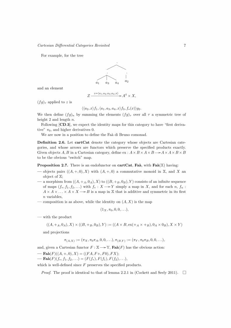
For example, for the tree

.

.

a1 a3 a4

.

a2

and an element

Zz=〈a1,a2,a3,a4,x〉 //A4 ×X,

(fg)τ applied to z is

〈〈a2, x〉f1, 〈a1, a3, a4, x〉f3, f∗(x)〉g2.We then define (fg)n by summing the elements (fg)τ over all τ a symmetric tree of

height 2 and length n.

Following [CD.3], we expect the identity maps for this category to have “first deriva-

tive” π0, and higher derivatives 0.

We are now in a position to define the Faa di Bruno comonad.

Definition 2.6. Let cartCat denote the category whose objects are Cartesian cate-

gories, and whose arrows are functors which preserve the specified products exactly.

Given objects A,B in a Cartesian category, define ex : A×B×A×B //A×A×B×Bto be the obvious “switch” map.

Proposition 2.7. There is an endofunctor on cartCat, Faa, with Faa(X) having:

— objects pairs ((A,+, 0), X) with (A,+, 0) a commutative monoid in X, and X an

object of X;

— a morphism from ((A,+A, 0A), X) to ((B,+B , 0B), Y ) consists of an infinite sequence

of maps (f∗, f1, f2, . . .) with f∗ : X // Y simply a map in X, and for each n, fn :

A× A× . . .× A×X // B is a map in X that is additive and symmetric in its first

n variables,

— composition is as above, while the identity on (A,X) is the map

(1X , π0, 0, 0, . . .),

— with the product

((A,+A, 0A), X)× ((B,+B , 0B), Y ) := ((A×B, ex(+A ×+B), 0A × 0B), X × Y )

and projections

π(A,X) := (πX , π0πA, 0, 0, . . .), π(B,Y ) := (πY , π0πB , 0, 0, . . .),

and, given a Cartesian functor F : X // Y, Faa(F ) has the obvious action:

— Faa(F )((A,+, 0), X) = ((FA,F+, F0), FX);

— Faa(F )(f∗, f1, f2, . . .) = (F (f∗), F (f1), F (f2), . . .),

which is well-defined since F preserves the specified products.

Proof. The proof is identical to that of lemma 2.2.1 in (Cockett and Seely 2011).

G.S.H. Cruttwell 8

Note that there are two key differences between the monad presented here and the one

presented in (Cockett and Seely 2011). In the version there, the base categories already

have all objects additive, and the action of the monad on a category X has objects pairs

(A,A). In our version, the base categories are mere categories with products, while the

action on a category X gives a category with objects pairs (A,X), with A a commutative

monoid.

In addition, in this more generalized setting, there is a natural comparison between

this endofunctor and the commutative monoid endofunctor, which does not appear at

the level considered in (Cockett and Seely 2011).

Definition 2.8. let cMon denote the endofunctor on cartCat which sends a category

X to its category of commutative monoids and additive maps between them (with its

obvious product structure).

Proposition 2.9. There is a natural transformation λ : cMon(X) // Faa(X), which

maps

(A,+, 0) 7→ ((A,+, 0), A)

and

Af //B 7→ (f, π0f, 0, 0, . . .).

Proof. λX(f) is a valid map in Faa(X) since f is additive. For each X, λX is a functor

since 1((A,+,0),A) = (1, π0, 0, . . .) and

λX(f)λX(g) = (f, π0f, 0, . . .)(g, π0g, 0, . . .)

= (fg, 〈π0f, π1f〉π0g, 0, . . .)= (fg, π0fg, 0, . . .)

= λX(fg).

It preserves products since the projections in Faa(X) are λX(π0), λX(π1). For naturality,

for a product-preserving functor F : X // Y we need the diagram

cMon(Y) Faa(Y)λY

//

cMon(X)

cMon(Y)

cMon(F )

��

cMon(X) Faa(X)λX // Faa(X)

Faa(Y)

Faa(F )

��

to commute. It is easy to see that on objects these two composite functors are equal,

while for an addition-and-0-preserving map f : (A,+A, 0A) // (B,+B , 0B) ∈ X,

λY(cMon(F )(f)) = λY(F (f)) = (F (f), π0F (f), F (0B), . . .)

(since the 0 in the codomain is F (0B)), while

Faa(F )(λX(f)) = Faa(F )(f, π0f, 0B , . . .) = (F (f), π0F (f), F (0B), . . .)

since F preserves the specified products. So λ is natural, as required.

Cartesian Differential Categories Revisited 9

Corollary 2.10. If (A,+, e) is a commutative monoid in X, then

(((A,+, 0), A), (+, π0+, 0, . . .), (0, π00, 0, . . .))

is a commutative monoid in Faa(X).

Proof. Since (A,+, 0) is commutative, (A,+, 0) is a commutative monoid in cMon(X),

and so gets sent by λX to a commutative monoid in Faa(X).

We can now describe the comonad structure of our generalized version of Faa, again

generalizing the work from (Cockett and Seely 2011). There is an obvious co-unit ε :

Faa(X) // X which maps (A,X) to X and f : (A,X) // (B, Y ) to f∗ : X // Y . The

co-multiplication δ is more complicated. On arrows it should be thought of giving an

abstract “derivative” of a map f = (f∗, f1, f2, . . .) : (A,X) // (B, Y ). On objects, it

will map (A,X) to ((A,A), (A,X)). For a map f = (f∗, f1, f2, . . .) : (A,X) // (B, Y ) in

Faa(X), note that δ(f) : ((A,A), (A,X)) // ((B,B), (B, Y )) will be a map in Faa2(X),

and so it will be a sequence of maps, each of which is itself a sequence of maps. There is

a natural choice for δ(f)∗: as its type should be a map (A,X) // (B, Y ) in Faa(X), we

can simply define δ(f)∗ as f .

For n ≥ 1, there is also a natural choice for (δ(f)n)∗: its type is An ×X //B, so we

simply take fn. For m ≥ 1, (δ(f)n)m has type

(An ×A)m × (An ×X) //B.

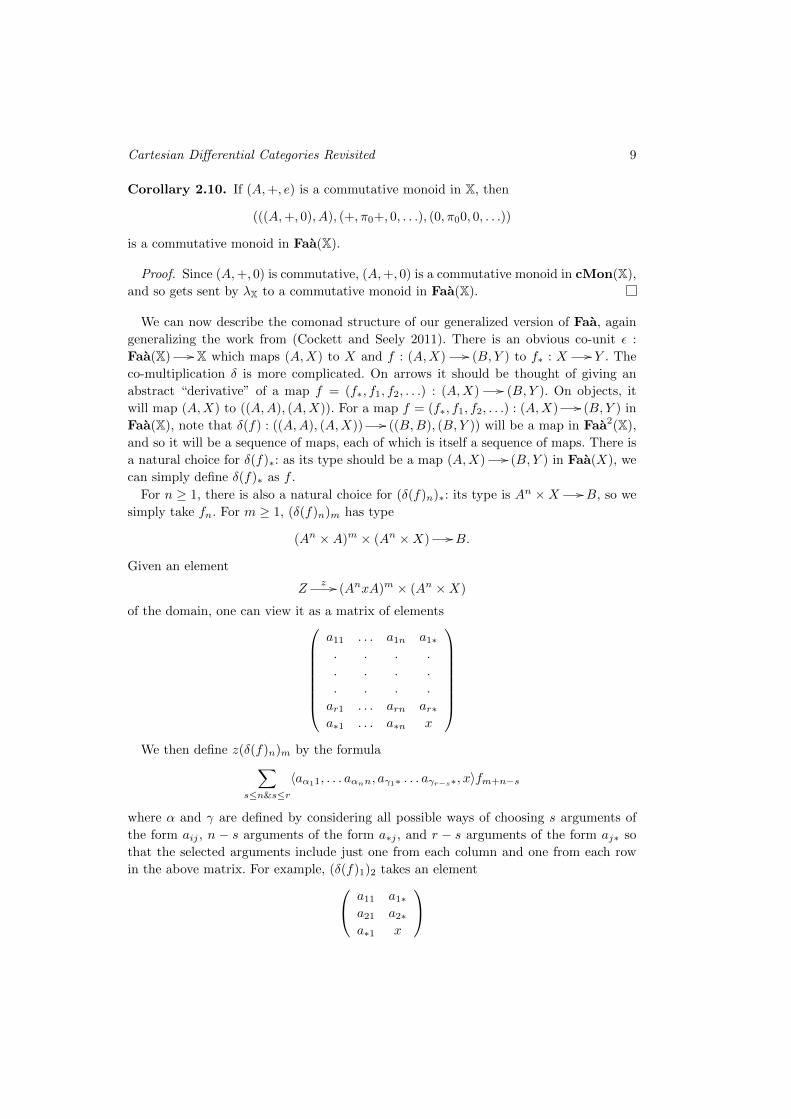
Given an element

Zz // (AnxA)m × (An ×X)

of the domain, one can view it as a matrix of elements

a11 . . . a1n a1∗. . . .

. . . .

. . . .

ar1 . . . arn ar∗a∗1 . . . a∗n x

We then define z(δ(f)n)m by the formula∑

s≤n&s≤r

〈aα11, . . . aαnn, aγ1∗ . . . aγr−s∗, x〉fm+n−s

where α and γ are defined by considering all possible ways of choosing s arguments of

the form aij , n − s arguments of the form a∗j , and r − s arguments of the form aj∗ so

that the selected arguments include just one from each column and one from each row

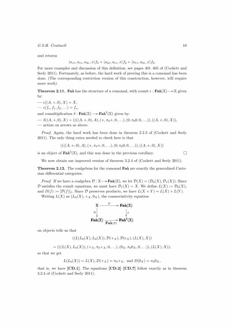
in the above matrix. For example, (δ(f)1)2 takes an element a11 a1∗a21 a2∗a∗1 x

G.S.H. Cruttwell 10

and returns

〈a∗1, a1∗, a2∗, x〉f3 + 〈a21, a1∗, x〉f2 + 〈a11, a2∗, x〉f2.For more examples and discussion of this definition, see pages 401–405 of (Cockett and

Seely 2011). Fortunately, as before, the hard work of proving this is a comonad has been

done. (The corresponding restriction version of this construction, however, will require

more work).

Theorem 2.11. Faa has the structure of a comonad, with counit ε : Faa(X) //X given

by:

— ε((A,+, 0), X) = X,

— ε(f∗, f1, f2, . . .) = f∗,

and comultiplication δ : Faa(X) // Faa2(X) given by:

— δ((A,+, 0), X) = ((((A,+, 0), A), (+, π0+, 0, . . .), (0, π00, 0, . . .)), ((A,+, 0), X)),

— action on arrows as above.

Proof. Again, the hard work has been done in theorem 2.2.2 of (Cockett and Seely

2011). The only thing extra needed to check here is that

((((A,+, 0), A), (+, π0+, 0, . . .), (0, π00, 0, . . .)), ((A,+, 0), X))

is an object of Faa2(X), and this was done in the previous corollary.

We now obtain our improved version of theorem 3.2.4 of (Cockett and Seely 2011).

Theorem 2.12. The coalgebras for the comonad Faa are exactly the generalized Carte-

sian differential categories.

Proof. If we have a coalgebra D : X //Faa(X), we let D(X) = (D0(X),D1(X)). Since

D satisfies the counit equations, we must have D1(X) = X. We define L(X) := D0(X),

and D(f) := [D(f)]1. Since D preserves products, we have L(X × Y ) = L(X)× L(Y ).

Writing L(X) as (L0(X),+X , 0X), the coassociativity equation

Faa(X) Faa2(X)Faa(D)

//

X

Faa(X)

D��

X Faa(X)D // Faa(X)

Faa2(X)

�

on objects tells us that

((L(L0(X), L0(X)),D(+X),D(eX), (L(X), X))

= (((L(X), L0(X)), (+X , π0+X , 0, . . .), (0X , π00X , 0, . . .)), (L(X), X)),

so that we get

L(L0(X)) = L(X), D(+X) = π0+X , and D(0X) = π00X ,

that is, we have [CD.1]. The equations [CD.2]–[CD.7] follow exactly as in theorem

3.2.4 of (Cockett and Seely 2011).

Cartesian Differential Categories Revisited 11

Conversely, if we have a generalized Cartesian differential category, we define

D(X) := (L(X), X)

and

D(f) := (f,D(f), D2(f), D3(f), . . .)

where

Dn(f) := 〈0, 0, . . . 0, π0, π1, . . . πn〉Dn(f).

Almost all of the work in showing that this is a coalgebra is in theorem 3.2.4 of (Cockett

and Seely 2011). The only thing left to check is that D(+) = (+, π0+, 0, . . .) and D(0) =

(0, π00, 0, . . .). But [CD.1] gives D(+)1 = π0+, and the higher terms are then 0, as

〈0, π0, π1, π2〉D2(+) = 〈0, π0, π1, π2〉D(π0+) = 〈0, π0, π1, π2〉π0π0D(+) = 0

and similarly for D(0).

Corollary 2.13. If X is a Cartesian category, then Faa(X) is a generalized Cartesian

differential category, with

D(f) = [δ(f)]1.

Of course, this is nothing more than stating that cofree coalgebras exist, but it is worth

highlighting this particular result, as it shows that there are innumerable examples of

generalized Cartesian differential categories. Note that Faa(X) has trivial differential

structure if and only if 1 is the only commutative monoid in X, as for example happens

if X is a poset with finite meets. But in most cases of interest (say, X = sets), Faa(X) is

highly non-trivial.

A more in-depth investigation of such cofree generalized Cartesian differential cate-

gories is clearly required; for now, we content ourselves with determining their linear

maps (this was not considered in (Cockett and Seely 2011)).

In a Cartesian differential category, a map f : X // Y is called linear if D(f) = π0f .

For a general map in a generalized Cartesian differential category, this is not possible,

as π0f is not even well-defined. But if L0(X) = X and L0(Y ) = Y , then the types do

match, and we can define what it means for such maps to be linear.

Definition 2.14. Say that an object X in a generalized Cartesian differential category

is a linear object if L0(X) = X. Say that map f : X // Y between linear objects is a

linear map if D(f) = π0f .

Recalling the definition of λ from proposition 2.9, we can now determine the linear

maps in cofree generalized Cartesian differential categories.

Proposition 2.15. The linear maps in Faa(X) are exactly those maps of the form λ(f)

for f an additive map from (A,+A, 0A) to (B,+B , 0B).

Proof. Note that the linear objects in Faa(X) are those objects of the form

λ(A,+A, 0A) = ((A,+A, 0A), A).

G.S.H. Cruttwell 12

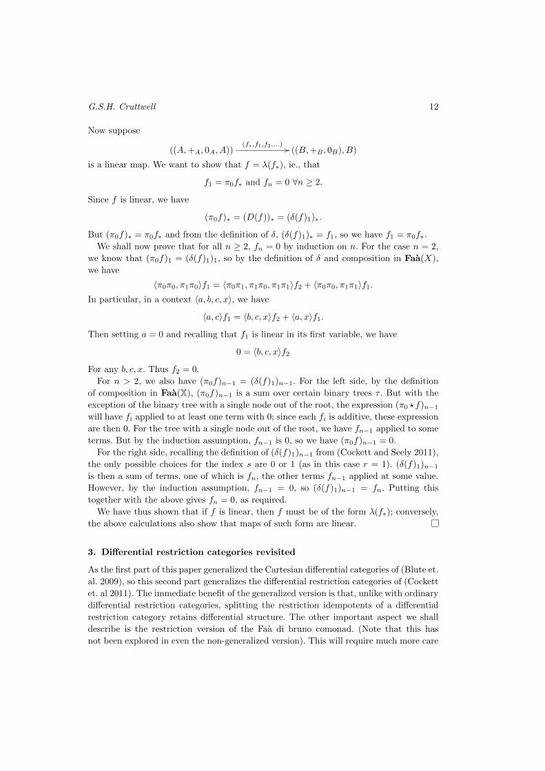
Now suppose

((A,+A, 0A, A))(f∗,f1,f2,...) // ((B,+B , 0B), B)

is a linear map. We want to show that f = λ(f∗), ie., that

f1 = π0f∗ and fn = 0 ∀n ≥ 2.

Since f is linear, we have

(π0f)∗ = (D(f))∗ = (δ(f)1)∗.

But (π0f)∗ = π0f∗ and from the definition of δ, (δ(f)1)∗ = f1, so we have f1 = π0f∗.

We shall now prove that for all n ≥ 2, fn = 0 by induction on n. For the case n = 2,

we know that (π0f)1 = (δ(f)1)1, so by the definition of δ and composition in Faa(X),

we have

〈π0π0, π1π0〉f1 = 〈π0π1, π1π0, π1π1〉f2 + 〈π0π0, π1π1〉f1.In particular, in a context 〈a, b, c, x〉, we have

〈a, c〉f1 = 〈b, c, x〉f2 + 〈a, x〉f1.

Then setting a = 0 and recalling that f1 is linear in its first variable, we have

0 = 〈b, c, x〉f2

For any b, c, x. Thus f2 = 0.

For n > 2, we also have (π0f)n−1 = (δ(f)1)n−1. For the left side, by the definition

of composition in Faa(X), (π0f)n−1 is a sum over certain binary trees τ . But with the

exception of the binary tree with a single node out of the root, the expression (π0 ?f)n−1will have fi applied to at least one term with 0; since each fi is additive, these expression

are then 0. For the tree with a single node out of the root, we have fn−1 applied to some

terms. But by the induction assumption, fn−1 is 0, so we have (π0f)n−1 = 0.

For the right side, recalling the definition of (δ(f)1)n−1 from (Cockett and Seely 2011),

the only possible choices for the index s are 0 or 1 (as in this case r = 1). (δ(f)1)n−1is then a sum of terms, one of which is fn, the other terms fn−1 applied at some value.

However, by the induction assumption, fn−1 = 0, so (δ(f)1)n−1 = fn. Putting this

together with the above gives fn = 0, as required.

We have thus shown that if f is linear, then f must be of the form λ(f∗); conversely,

the above calculations also show that maps of such form are linear.

3. Differential restriction categories revisited

As the first part of this paper generalized the Cartesian differential categories of (Blute et.

al. 2009), so this second part generalizes the differential restriction categories of (Cockett

et. al 2011). The immediate benefit of the generalized version is that, unlike with ordinary

differential restriction categories, splitting the restriction idempotents of a differential

restriction category retains differential structure. The other important aspect we shall

describe is the restriction version of the Faa di bruno comonad. (Note that this has

not been explored in even the non-generalized version). This will require much more care

Cartesian Differential Categories Revisited 13

than the non-restriction generalization given in the previous section, as we have to ensure

everything works well with the restriction structure.

As noted in the introduction, since every category is a restriction category with trivial

restriction structure, the results of the previous section are in fact corollaries of the

results presented in this section. However, we have presented the basic non-restriction

version first to help the reader gain an understanding of the constructions and definitions

involved before seeing how the structure interacts with restrictions.

To begin, we first recall the definition of a restriction category from (Cockett and Lack

2002):

Definition 3.1. Given a category, X, a restriction structure on X gives for each map

Af−→ B, a map, A

f−→ A, satisfying four axioms:

[R.1] f f = f ;

[R.2] If dom(f) = dom(g) then g f = f g ;

[R.3] If dom(f) = dom(g) then g f = g f ;

[R.4] If dom(h) = cod(f) then fh = fh f .

A category with a specified restriction structure is a restriction category.

The canonical example is that of partial functions between sets, where, given a partial

function f : X // Y , f is essentially the identity on the domain of definition of f :

f(x) =

{x if f(x) defined

undefined otherwise.

Recall also that map in a restriction category is said to be total if f = 1, while a

restriction idempotent is a map e : X //X such that e = e.

The following results from (Cockett and Lack 2002) are useful when doing calculations

with the restriction operation:

Proposition 3.2. If X is a restriction category then:

(i) f is idempotent;

(ii) f fg = fg ;

(iii) fg = fg ;

(iv) f = f ;

(v) f g = f g ;

(vi) If f is monic then f = 1 (and so in particular 1 = 1);

(vii) f g = g implies g = f g .

In addition, we need to recall what it means for a restriction category to have finite

products. Thinking about the category of sets and partial functions, one sees that the

ordinary product of sets X and Y will not a be a categorical product in the category

of sets and partial functions. Given maps f : Z // X, g : Z // Y , we will not have

〈f, g〉π0 = f , as 〈f, g〉 will only be defined where both f and g are. However, 〈f, g〉π0 will

be equal to f on this smaller domain of definition. This leads to the following definitions

in an abstract restriction category.

G.S.H. Cruttwell 14

Definition 3.3. Given parallel maps f, g : A //B in a restriction category, write f ≤ gif f g = f , and write f ^ g if f g = g f .

Intuitively, f ≤ g captures the idea of g being the same function as f , but on a larger

domain of definition, while f ^ g captures the idea of f and g being equal wherever

they are both defined. One can check that ≤ is a partial order. We can now define what

it means for a restriction category to have restriction products.

Definition 3.4. Let X be a restriction category. A restriction terminal object is an

object T in X such that for any object A, there is a unique total map !A : A −→ T

which satisfies !T = 1T . These maps must also satisfy the property that for any map

f : A −→ B, f !B ≤ !A, i.e. f !B = f !B !A = f !B !A = f !A.

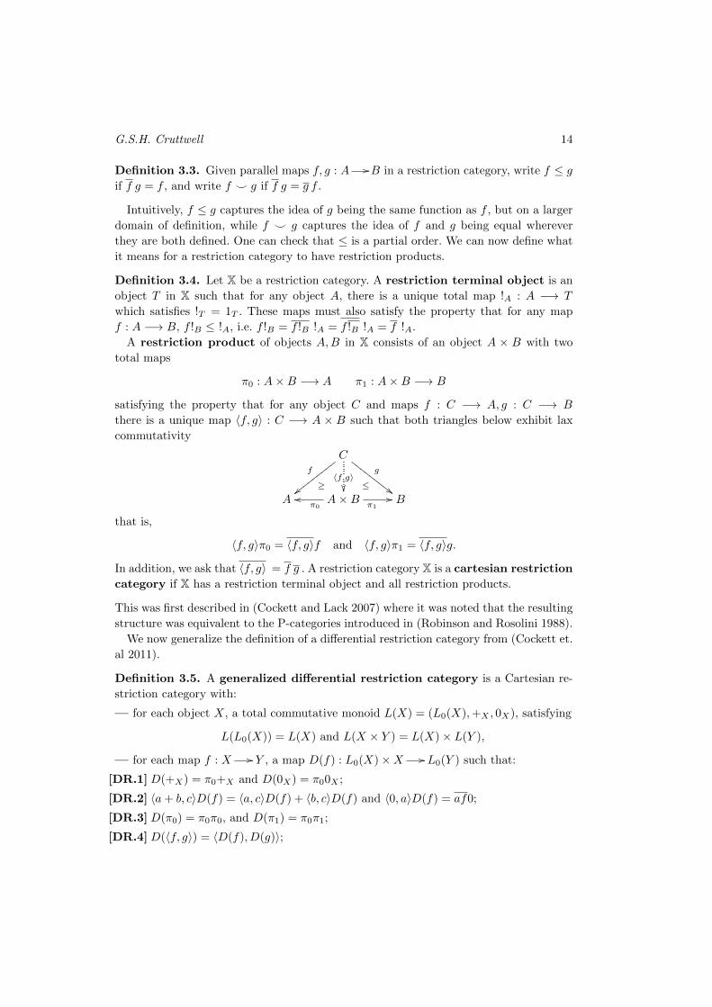
A restriction product of objects A,B in X consists of an object A × B with two

total maps

π0 : A×B −→ A π1 : A×B −→ B

satisfying the property that for any object C and maps f : C −→ A, g : C −→ B

there is a unique map 〈f, g〉 : C −→ A × B such that both triangles below exhibit lax

commutativity

Cf

||xxxxxxxxx

g

##FFF

FFFF

FF

〈f,g〉��≥ ≤

A A×Bπ0

ooπ1

// B

that is,

〈f, g〉π0 = 〈f, g〉f and 〈f, g〉π1 = 〈f, g〉g.

In addition, we ask that 〈f, g〉 = f g . A restriction category X is a cartesian restriction

category if X has a restriction terminal object and all restriction products.

This was first described in (Cockett and Lack 2007) where it was noted that the resulting

structure was equivalent to the P-categories introduced in (Robinson and Rosolini 1988).

We now generalize the definition of a differential restriction category from (Cockett et.

al 2011).

Definition 3.5. A generalized differential restriction category is a Cartesian re-

striction category with:

— for each object X, a total commutative monoid L(X) = (L0(X),+X , 0X), satisfying

L(L0(X)) = L(X) and L(X × Y ) = L(X)× L(Y ),

— for each map f : X // Y , a map D(f) : L0(X)×X // L0(Y ) such that:

[DR.1] D(+X) = π0+X and D(0X) = π00X ;

[DR.2] 〈a+ b, c〉D(f) = 〈a, c〉D(f) + 〈b, c〉D(f) and 〈0, a〉D(f) = af0;

[DR.3] D(π0) = π0π0, and D(π1) = π0π1;

[DR.4] D(〈f, g〉) = 〈D(f), D(g)〉;

Cartesian Differential Categories Revisited 15

[DR.5] D(fg) = 〈D(f), π1f〉D(g);

[DR.6] 〈〈a, 0〉, 〈c, d〉〉D2(f) = c〈a, d〉D(f);

[DR.7] 〈〈0, b〉, 〈c, d〉〉D2(f) = 〈〈0, c〉, 〈b, d〉〉D2(f);

[DR.8] D(f) = (1× f)π0 = π1f π0;

[DR.9] D(f) = 1× f = π1f .

Note the addition of a restriction in axioms [DR.2] and [DR.6]: this is necessary since

we must keep track of the partiality of the maps that are lost across the equality. The

8th and 9th axioms demand that the differential operator be total in its first variable.

Remark 3.6. Any generalized Cartesian differential category is a generalized differential

restriction category, when equipped with the trivial restriction structure (f = 1 for all

f). Any differential restriction category is a generalized differential restriction category,

with L(X) = X for each X.

The standard example of a non-trivial differential restriction category is:

Example 3.7. Smooth functions defined on open subsets of Rn.

More examples, such as differential restriction categories of rational functions, can be

found in (Cockett et. al 2011).

One of the reasons for generalizing differential restriction categories is the following

construction. Recall from (Cockett and Lack 2002) that if X is a restriction category, then

the restriction idempotent splitting of X, Kr(X), is a restriction category with:

— objects restriction idempotents (X, e = e );— a map f : (X, e1) // (Y, e2) is a map f : X // Y such that e1fe2 = f ;— restriction and composition as in X, and 1(X,e) := e.

One problem with differential restriction categories is that even if X is a differential

restriction category, Kr(X) need not be: because of [DR.9], the derivative must be total

in the first variable, and so the derivative of a map f : (X, e1) // (Y, e2) cannot have

domain (X, e1) × (X, e1). With generalized differential restriction categories, this is no

longer a problem, as we can set L(X, e1) = (L(X), 1).

Proposition 3.8. If X is a generalized differential restriction category then Kr(X) is

also, with

L(X, e) := (L(X), 1) and D(f) := D(f).

Proof. The only thing to check is that D(f) is a valid map in the restriction idempotent

splitting category. Suppose f : (X, e1) // (Y, e2). We are claiming that D(f) is a valid

map from (L0(X)×X, 1× e1) to (L0(Y ), 1). So consider

(1× e1)D(f) = (1× e1)D(f)D(f) = (1× e1)(1× f )D(f) = (1× f )D(f) = D(f)

by [DR.9] and the fact that e1fe2 = f .

For example, when X is the differential restriction category of partial smooth maps

between Cartesian spaces, Kr(X) is a generalized differential restriction category whose

objects are open subsets of Cartesian spaces.

G.S.H. Cruttwell 16

Corollary 3.9. If X is a differential restriction category, then the total maps of Kr(X)

form a generalized Cartesian differential category.

As noted in the introduction, this shows that the categories whose objects are open

subsets of Rn, and whose maps are (total) smooth maps between them, forms a general-

ized Cartesian differential category.

3.1. Faa di bruno - restriction version

In this section, we extend the Faadi Bruno comonad to work with restriction categories.

Recall from earlier that in Faa(X), given two composable maps f : (A,X) // (B, Y ),

g : (B, Y ) // (C,Z), we have

(fg)n :=∑

(f ? g)τ ,

where the sum is over each tree τ of length 2 and width n. For such a tree τ , the term

(f ? g)τ term is of the form

〈p1fi1 , p2fi2 , . . . pkfik , πnf∗〉gk

where k, each ij , and pi all depend on the tree τ , and each pi is of the form 〈πj1 , πj2 , . . . πji1 , πn〉.Our first goal is to prove the following

Theorem 3.10. Given a Cartesian restriction category X, there is a Cartesian restriction

category Faa(X) which has:

— objects pairs ((A,+, 0), X), where X is an object of X and (A,+, 0) is a (total)

commutative monoid in X;

— maps sequences

(f∗, f1, f2, . . .) : (A,X) // (B, Y )

where f∗ : X // Y , and for each n ≥ 1, fn : (A)n ×X // B with fn additive and

symmetric in the first n variables and

fn = 1× f∗ = πnf∗ ;

— composition and identities are defined as in the total case;

— restriction given by

(f∗, f1, f2, . . .) := (f∗ , π1f∗ π0, π2f∗ 0, π3f∗ 0 . . .).

We will begin with a lemma. When working with a putative restriction category, it is

often helpful to first determine what a map of the form f g looks like.

Lemma 3.11. With the above definition of f , for n ≥ 1 and maps f : X // A,

g : X //B, we have

(f g)n = πnf∗ gn.

Proof. Recalling the definition of composition as above, we have (f ?g)τ is of the form

〈p1f i1 , p2f i2 , . . . pkf ik , πnf ∗〉gk

Cartesian Differential Categories Revisited 17

But for any i ≥ 1, the expression pjf ij is a restriction of 0, and with the exception of

the tree with n branches out of the root, that expression occurs at least once. Then since

each gk is additive in each of the first n variables, we have

(f ? g)τ = πnf∗ g∗ 0 = πnf∗ πng∗ 0.

For that one tree τ0 with n branches out of the root,

(f ? g)τ0 = 〈〈π0, πn〉(f )1, 〈π1, πn〉(f )1, . . . 〈πn−1, πn〉(f )1, πnf∗〉gn.

But for each i ∈ {1 . . . n− 1},

〈πi, πn〉(f )1 = 〈πi, πn〉π1f∗ π0 = πnf∗ 〈πi, πn〉π0 = πnf∗ πi,

so that

(f ? g)τ0 = πnf∗ 〈π0, π1, . . . πn〉gn = πnf∗ gn

Thus, the sum over all trees τ equals

πnf∗ gn + πnf∗ πng∗ 0 = πnf∗ πng∗ gn = πnf∗ gn

by assumption on gn. Thus we have

(f g)n = πnf∗ gn,

as required.

Proposition 3.12. Faa(X) is a restriction category.

Proof.

We first need to check that the identities, composites, and restriction satisfy the added

requirement on the restriction of its components. That identities satisfy the requirement

is obvious, since 1(A,x) = (1, π0, 0A, . . .) and both π0 and 0A are total.

To check that the composite of two maps f : (A,X) // (B, Y ), g : (B, Y ) // (C,Z)

satisfies the restriction requirement, as above, recall that (fg)n =∑

(f ? g)τ . Since

x+ y = x y , to calculate (fg)n , we need to calculate each (f ? g)τ . For such a tree τ ,

this term is of the form

〈p1fi1 , p2fi2 , . . . pkfik , πnf∗〉gkwhere k, each ij , and pi all depend on the tree τ . In particular, however, each pm is of

the form 〈πj1 , πj2 , . . . πjim , πn〉 (where again each jl depends on τ) so we have

pmfim

= 〈πj1 , πj2 , . . . πjim , πn〉fim= 〈πj1 , πj2 , . . . πjim , πn〉fim= 〈πj1 , πj2 , . . . πjim , πn〉πimf∗= 〈πj1 , πj2 , . . . πjim , πn〉πimf∗= πnf∗

G.S.H. Cruttwell 18

Then we can calculate, for any such tree τ ,

(f ? g)τ = 〈p1fi1 , p2fi2 , . . . pkfik , πnf∗〉gk= 〈p1fi1 , p2fi2 , . . . pkfik , πnf∗〉gk= 〈p1fi1 , p2fi2 , . . . pkfik , πnf∗〉πng∗= 〈p1fi1 , p2fi2 , . . . pkfik , πnf∗〉πng∗= p1fi1 p2fi2 . . . pkfik πnf∗g∗

= πnf∗ πnf∗ . . . πnf∗ πnf∗g∗

= πnf∗g∗

= πn(fg)∗

so that we get (fg)n = πn(fg)∗ , as required.

Each restriction map satisfies the requirement on the restriction of its components

since

πnf∗ π0 = πn f∗ = πnf∗ 0

as 0 and π0 are both total.

That Faa(X) is a category is as in (Cockett and Seely 2011). We now turn to checking

the restriction axioms. As the equality of ∗ terms follows directly, we will simply check

for the n ≥ 1 terms. For [R.1], by lemma 3.11,

(f f)n = πnf∗ fn = fn

by assumption on fn. For [R.2], for n ≥ 2, by lemma 3.11, we have

(f g )n = πnf∗ πng∗ 0 = πng∗ πnf∗ 0 = (g f )n

and n = 1 is similar. For [R.3], again by lemma 3.11, we have

(f g )1 = π1(f g)∗ 0 = π1f∗ g 0 = π1f∗ π1g 0 = π1f∗ π1g∗ 0

which is the required value, by the calcuation for [R.2]; again n = 1 is similar.

For [R.4], we need to find the nth term of fg . This time, for any tree τ with the

exception of the tree with a single node out of the root, we have

(f ? g )τ = 〈p1fi1 , p2fi2 , . . . πnf∗〉πng∗ 0

= 〈p1fi1 , p2fi2 , . . . πnf∗〉πng∗ 〈p1fi1 , p2fi2 , . . . πnf∗〉 0

= πnf∗g∗ πnf∗ 0

= πnf∗g∗ 0

For that one tree τ1 with a single node out of the root, we have

(f ? g )τ1 = 〈fn, πnf∗〉π1g∗ π0 = πnf∗gn fn.

Then summing over all trees τ gives

(fg )n = πnf∗g∗ 0 + πnf∗gn fn = πnf∗gn fn.

Cartesian Differential Categories Revisited 19

Conversely, by lemma 3.11, we have

(fg f)n = πn(fg)∗ fn = πnf∗g∗ fn

so that [R.4] is satisfied, as required.

To prove that Faa(X) is a Cartesian restriction category, we need to determine which

maps are total, and when ≤ and ^ hold.

Proposition 3.13. In the restriction category Faa(X), for maps f, g : (X,A) // (Y,B):

(i) f is total if and only if f∗ is total;

(ii) f ≤ g if and only if f∗ ≤ g∗ and fn ≤ gn for each n ≥ 1;

(iii) f ^ g if and only if f∗ ^ g∗ and fn ^ gn for each n ≥ 1.

Proof.

(i)If f is total, then in particular (f )∗ = 1, so f∗ is total. Conversely, if f∗ is total, then

for n ≥ 2,

(f )n = πnf∗ 0 = πn 0 = 0

and similarly (f )1 = π0, so that f is total.

(ii)Recall that f ≤ g means f g = f . So f ≤ g if and only if f∗ ≤ g∗ and for each n ≥ 1,

(f g)n = fn. But by lemma 3.11,

(f g)n = πnf∗ gn = fn gn

by assumption on fn. Thus f ≤ g if and only if f∗ ≤ g∗ and for each n ≥ 1, fn ≤ gn.

(iii)Recall that f ^ g means f g = g f . The result then follows as in (ii).

We can now prove the following.

Proposition 3.14. With product structure as in the total case:

πi = (πi, π0πi, 0, 0, . . .), 〈f, g〉n := 〈fn, gn〉,

Faa(X) is a Cartesian restriction category.

Proof. We first need to show 〈f, g〉π0 ≤ f , so consider the term (〈f, g〉π0)n. As in the

proof of [R.4] in Theorem 3.10, for any tree τ with the exception of the tree τ1 which

has a single node coming out of the root, (〈f, g〉 ? π0)τ is of the form

〈p1〈f, g〉i1 , p2〈f, g〉i2 , . . . πn〈f, g〉∗〉0= p1〈f, g〉i1 p2〈f, g〉i2 . . . πn〈f, g〉∗ 0

= πn〈f∗, g∗〉 0= πnf∗ πng∗ 0

G.S.H. Cruttwell 20

while for τ1,

(〈f, g〉 ? π0)τ1 = 〈(〈f, g〉n, πn〈f, g〉∗〉π0π0= 〈〈fn, gn〉, πn〈f∗, g∗〉〉π0π0= gn πnf∗ πng∗ fn

= gn fn (by assumption on gn)

Thus

(〈f, g〉π0)n = πnf∗ πng∗ 0 + gn fn = gn fn,

so that by lemma 3.13, 〈f, g〉π0 ≤ f , as required; π1 is similar.

We also need to show that 〈f, g〉 = f g . For n ≥ 2, consider

(〈f, g〉 )n = πn〈fg〉∗ 0 = πn〈f∗, g∗〉 0 = πnf∗ πng∗ 0

while by lemma 3.11,

(f g )n = πnf∗ (g )n = πnf∗ πng∗ 0,

and n = 1 is similar, so that 〈f, g〉 = f g , as required.

This completes the proof of theorem 3.10. We now turn to the monad structure of Faa.

Proposition 3.15. Faa extends to an endofunctor on the category of Cartesian re-

striction categories (where the maps are those functors which preserve products and

restrictions exactly), where we define

Faa(F )(f∗, f1, f2, . . .) := (F (f∗), F (f1), F (f2), . . .)

Proof. The only thing to check is that Faa(F ) satisfies the restriction requirement on

its components:

F (fn) = F (fn ) = F (πnf∗ ) = πnF (f∗)

since F preserves restrictions and products exactly.

Proposition 3.16. The endofunctor Faa has the structure of a comonad, with counit

ε : Faa(X) // X given by:

— ε((A,+, 0), X) = X,

— ε(f∗, f1, f2, . . .) = f∗,

and comultiplication δ : Faa(X) // Faa2(X) given by:

— δ((A,+, 0), X) = (((A,+, 0), A), (+, π0+, 0, . . .), (0, π00, 0, . . .)), ((A,+, 0), X))),

— action on arrows as in the total case.

Proof. There are only a few additional things to check here:

(i)that ε preserves restrictions;

(ii)that δ(f) is a valid arrow in Faa2(X);

(iii)that δ preserves restrictions.

The first part is obvious, as by definition (f )∗ = f∗ .

Cartesian Differential Categories Revisited 21

For (ii), we need to show that

δ(f)n = πnδ(f)∗ ,

so we need to show that they are equal in each component. For m ≥ 2, we have

(δ(f)n)m

= πm(δ(f)n)∗ 0 (by definition of restriction)

= πmfn 0 (by definition of δ(f))

= πmfn 0

= πmπnf∗ 0 (by assumption on fn)

= πmπnf∗ 0

while

(πnδ(f)∗ )m = πm(πnδ(f)∗)∗ 0 = πmπnf∗ 0

by definition of δ(f), so that they are equal, as required. The case m = 1 and the ∗component are similar.

For (iii), we need δ(f ) = δ(f) , so in particular we need for each n,m ≥ 1,

((δ(f ))n)m = ((δ(f) )n)m.

For n,m ≥ 2, starting with the right side, we have

((δ(f) )n)m

= (πnδ(f)∗ 0)m (by definition of restriction)

= πm(πnδ(f)∗)∗ 0 (by lemma 3.11)

= πmπnf∗ 0 (by definition of δ).

For ((δ(f ))n)m, recalling the definition of δ the previous section, we see that ((δ(f ))n)mis a sum of terms of the form

〈πα1,β1, πα2,β2

, . . . , πm〉πnf∗ 0,

for certain indices αi, βj . The particular form of these indices is not important however,

as in each case we have

〈πα1,β1 , πα2,β2 , . . . , πm〉πnf∗ 0

= 〈πα1,β1, πα2,β2

, . . . , πm〉πnf∗ 〈πα1,β1, πα2,β2

, . . . , πm〉0= πmπnf∗ 0 (since projections are total)

so that the sum is also πmπnf∗ 0, and we have ((δ(f ))n)m = ((δ(f) )n)m. The cases for

m,n equalling 1 or ∗ or similar, so δ(f ) = δ(f) , as required.

Theorem 3.17. The coalgebras for the comonad (Faa, ε, δ) are exactly the generalized

differential restriction categories.

Proof. As before, if we have a coalgebraD : X //Faa(X), we letD(X) = (D0(X),D1(X)).

G.S.H. Cruttwell 22

Since D satisfies the counit equations, we must have D1(X) = X. We define L(X) :=

D0(X), and D(f) := [D(f)]1.

For the most part, the fact that this operation satisfies the differential restriction

axioms is exactly as before, with a few minor modifications. Since D(f) := [D(f)]1 is a

map in Faa(X), we must have D(f)1 = π1D(f)∗ = π1f . Since D preserves restrictions,

we have

D(f ) = D(f )1 = (D(f) )1 = π1f π0.

Thus, we have both of the added differential restriction axioms.

Note that D(f) being additive in its first variable means that

〈0, x〉D(f) = 〈0, x〉[D(f)]1 0 = xf∗ 0 = xf 0,

giving [DR.2]. Similarly, as on pg. 414 of (Cockett and Seely 2011), we get [DR.6] by

setting a certain term equal to 0; the extra restriction term then comes out when we

project.

Conversely, if we have a generalized Cartesian differential category, and define

D(f) := (f,D(f), D2(f), D3(f), . . .)

where

Dn(f) := 〈0, 0, . . . 0, π0, π1, . . . πn〉Dn(f),

the only thing we need to check here is that D(f) is a valid map in Faa(X). That is, we

need Dn(f) = πnf . But since D(f) = π1f , we have Dn(f) = π1π1 . . . π1f (n π1’s), so

that

Dn(f) = 〈0, 0, . . . 0, π0, π1, . . . πn〉Dn(f) = πnf ,

as required.

Corollary 3.18. If X is a Cartesian restriction category, then Faa(X) is a generalized

differential restriction category, with

D(f) := [δ(f)]1.

Again, this is nothing more than stating that free coalgebras exist; but it highlights

the fact that there are many instances of generalized differential restriction categories

beyond the standard examples.

References

Blute, R., Cockett, J and Seely, R. Differential categories. Mathematics Structures in Computer

Science, 16, 1049–1083, 2006.

Blute, R., Cockett, J and Seely, R. Cartesian differential categories. Theory and Applications

of Categories, 22, 622–672, 2009.

Blute, R., Ehrhard, T., and Tasson, C. A convenient differential category. To appear in Cahiers

de Topologie et Geometrie Differential Categoriques, 2011.

Cockett, R., Cruttwell, G., and Gallagher, J. Differential restriction categories. Theory and

Applications of Categories, 25, pg. 537–613, 2011.

Cartesian Differential Categories Revisited 23

Cockett, R. and Lack, S. Restriction categories I: categories of partial maps. Theoretical computer

science, 270 (2), 223–259, 2002.

Cockett, J. and Lack, S. Restriction categories III: colimits, partial limits, and extensivity.

Mathematical Structures in Computer Science, 17, 775–817, 2007.

Cockett, R. and Cruttwell, G. Differential structure, tangent structure, and

SDG. To appear in Applied Categorical Structures; available online at

http://geoff.reluctantm.com/publications.html.

Cockett, J and Seely, R. The Faa di bruno construction. Theory and applictions of categories,

25, 393–425, 2011.

Ehrhard, T., and Regnier, L. The differential lambda-calculus. Theoretical Computer Science,

309 (1), 1–41, 2003.

Kock, A. Synthetic Differential Geometry, Cambridge University Press (2nd ed.). Also available

at http://home.imf.au.dk/kock/sdg99.pdf, 2006.

Manzonetto, G. What is a categorical model of the differential and the resource λ-calculi?

Mathematical Structures in Computer Science, 22(3):451–520, 2012.

Laird, J, Manzonetto, G. and McCusker, G. Constructing differential categories and decon-

structing categories of games. Information and Computation, vol. 222, 247–264, 2013.

Robinson, E. and Roslini, G. Categories of partial maps. Information and Computation, vol. 79,

94–13, 1988.

Rosicky, J. Abstract tangent functors. Diagrammes, 12, Exp. No. 3, 1984.