CARNEGIE MELLON UNIVERSITYusers.ece.cmu.edu/~koopman/thesis/shelton.pdf · CARNEGIE MELLON UNIVERSITY ... 6.1 Mobot Navigation Problem ... Figure 3.7. Temporal Redundancy and Recovery

CARNEGIE MELLON UNIVERSITY

SCALABLE GRACEFUL DEGRADATION FORDISTRIBUTED EMBEDDED SYSTEMS

A DISSERTATIONSUBMITTED TO THE GRADUATE SCHOOL

IN PARTIAL FULFILMENT OF THE REQUIREMENTS

for the degree

DOCTOR OF PHILOSOPHY

in

ELECTRICAL AND COMPUTER ENGINEERING

by

Charles Preston Shelton

Pittsburgh, PennsylvaniaJune, 2003

Copyright 2003 by Charles P. Shelton. All rights reserved.

Abstract

Distributed embedded computer systems are at the heart of many safety-critical

systems such as airplanes, automobiles, and elevators. These systems have higher

dependability requirements than general-purpose computer systems, as a system

failure can cause human injury. However, these systems typically also have tight

cost constraints, meaning there is a limit on the amount of design effort and

redundant resources that can be spent making the system dependable. Traditional

fault tolerance techniques of installing multiple identical backup systems may be

cost prohibitive. Additionally, demand for more sophisticated system features has

led to significantly more complex software being incorporated into these systems,

and software design defects have become a major impediment to system

dependability.

Graceful degradation mechanisms can potentially provide increased system

dependability without having to provide redundant system resources. A gracefully

degrading system tolerates partial system failures by providing reduced

functionality with the remaining available system resources. In general, distributed

embedded systems are designed to optimize performance and functionality with

complex control algorithms and high quality sensors and actuators. The resources

already designed into the system can provide some level of redundancy because not

all of these system optimizations are required for the system to satisfy its primary

requirements. Graceful degradation can exploit existing resources to provide

increased dependability when partial system failures occur.

Designing a gracefully degrading complex software system is a significant

challenge. Existing best practice consists of specifying all possible combinations of

Abstract iii

system failures, and designing a distinct system response for each combination. For

a system with N failure modes, the design effort required for an ideal gracefully

degrading system is O(2N) which is clearly intractable for a complex distributed

embedded system.

This thesis presents a scalable approach to building gracefully degrading

distributed embedded systems. We define graceful degradation in terms of system

utility: a generic measure of the system’s ability to satisfy its functional and

dependability requirements. An ideal gracefully degrading system minimizes the

cumulative loss of system utility as successive system failures occur. We present a

system model that enables scalable specification of system-wide graceful

degradation. Our model views a distributed embedded system as a set of

components that are either software components, sensors, or actuators. A system

with N components that can each fail independently has 2N possible distinct system

failure configurations, one for each possible combination of failed components.

Defining the system’s ability to gracefully degrade would traditionally require

specifying the relative system utility of all 2N possible failure combinations. We

avoid this exponential complexity by exploiting the structure in the system’s

architecture to partition components into subsystems. We view each subsystem as a

configuration of components that changes utility when components are removed

due to failure or added via repair. We then view the system as a composition of

subsystems that each contribute to overall system utility. Our model reduces the

complexity of the system utility analysis from O(2N) to O(N*2k) where k is the

maximum number of components in any one subsystem.

Abstract iv

We apply our system model to representative system architectures and identify

some design techniques that can improve graceful degradation. We apply these

design techniques to two distributed embedded systems and demonstrate how they

enable scalable graceful degradation and increased system dependability. Our

model also allows us to evaluate traditional fault tolerance techniques in terms of

their ability to provide graceful degradation, and we can explicitly identify tradeoffs

between the cost of graceful degradation mechanisms, in terms of design effort and

redundant resources, and system dependability.

Abstract v

Acknowledgments

This thesis is dedicated to my wife, Tricia, without whom I could never have come

so far so fast. Her love and support have sustained me through the arduous process

of graduate school. I would also like to thank my parents and extended family, who

have always believed in me. Also, my new “Pittsburgh Family” of in-laws,

especially my mother- and father-in-law, have given me a support system that I

needed so much and never imagined was possible away from home.

I thank my advisor, Philip Koopman, for all of the advice, guidance, and

encouragement he has given me. This work would not have been possible without

him. Also, I thank my committee members, Alan Baum, Bruce Krogh, and David

Garlan, who provided time and support to meet with me and give me constructive

criticism. My fellow students have made my graduate school experience both

enjoyable and memorable. Thank you all for your help and support.

Graduate school is not free, and I appreciate all of the organizations that have

provided financial support for my research. This work was sponsored by Lucent

Technologies, the General Motors Collaborative Research Laboratory at Carnegie

Mellon University, the High De pend abil ity Com puting Pro gram from NASA Ames

co op er a tive agree ment NCC-2-1298, and the Pennsylvania Infrastructure

Technology Alliance.

Acknowledgments vi

Table of Contents

Abstract . . . . . . . . . . . . . . . . . . . . . . . . . . . . . . . . . . . . iiiAcknowledgments . . . . . . . . . . . . . . . . . . . . . . . . . . . . . . . vi

1 Introduction. . . . . . . . . . . . . . . . . . . . . . . . . . . . . . . . . . 11.1 Problem Statement . . . . . . . . . . . . . . . . . . . . . . . . . . . . . . . . . . . . . . . 31.2 Thesis Contributions . . . . . . . . . . . . . . . . . . . . . . . . . . . . . . . . . . . . . 81.3 Sys tem Context . . . . . . . . . . . . . . . . . . . . . . . . . . . . . . . . . . . . . . . . . 81.4 The sis Out line . . . . . . . . . . . . . . . . . . . . . . . . . . . . . . . . . . . . . . . . . 11

2 Related Work . . . . . . . . . . . . . . . . . . . . . . . . . . . . . . . . 132.1 Graceful Degradation. . . . . . . . . . . . . . . . . . . . . . . . . . . . . . . . . . . . 132.2 Dependability and Fault Tolerance . . . . . . . . . . . . . . . . . . . . . . . . . 152.3 Embedded Systems . . . . . . . . . . . . . . . . . . . . . . . . . . . . . . . . . . . . . 182.4 Software Architecture . . . . . . . . . . . . . . . . . . . . . . . . . . . . . . . . . . . 19

3 System Model for Graceful Degradation . . . . . . . . . . . . . . . . . 213.1 Data Flow and De pend ency Graph . . . . . . . . . . . . . . . . . . . . . . . . . 233.2 Acme Specification of the Software System View . . . . . . . . . . . . . 283.3 Hardware Al lo ca tion Diagram. . . . . . . . . . . . . . . . . . . . . . . . . . . . . 303.4 Util ity Model . . . . . . . . . . . . . . . . . . . . . . . . . . . . . . . . . . . . . . . . . . 323.5 Scal able Gen er a tion of the System Util ity Function . . . . . . . . . . . . 363.6 As sump tions of Our Model . . . . . . . . . . . . . . . . . . . . . . . . . . . . . . . 413.7 Tra di tional Fault-Tol er ance Tech niques . . . . . . . . . . . . . . . . . . . . . 45

3.7.1 Hard ware Re dun dancy . . . . . . . . . . . . . . . . . . . . . . . . . . . 453.7.2 Re cov ery Blocks and Tem po ral Re dun dancy . . . . . . . . . . 473.7.3 Multi-Ver sion Software Redundancy . . . . . . . . . . . . . . . . 483.7.4 Self-Check ing Programming. . . . . . . . . . . . . . . . . . . . . . . 503.7.5 An a lytic Redundancy . . . . . . . . . . . . . . . . . . . . . . . . . . . . 513.7.6 Sim plex Ar chi tec ture. . . . . . . . . . . . . . . . . . . . . . . . . . . . . 53

3.8 Con clu sions . . . . . . . . . . . . . . . . . . . . . . . . . . . . . . . . . . . . . . . . . . . 56

4 Architectural Properties for Graceful Degradation . . . . . . . . . . . 584.1 System Description . . . . . . . . . . . . . . . . . . . . . . . . . . . . . . . . . . . . . 604.2 Specification of the System Utility Function. . . . . . . . . . . . . . . . . . 624.3 Mechanisms that Contribute to Graceful Degradation . . . . . . . . . . 68

4.3.1 Well-Defined System Component Interfaces. . . . . . . . . . . 684.3.2 Targeted Redundancy for Critical Subsystems . . . . . . . . . 71

Table of Contents vii

4.3.3 Heterogeneous Redundancy . . . . . . . . . . . . . . . . . . . . . . . 724.3.4 Component Robustness to Loss of Inputs . . . . . . . . . . . . . 74

4.4 Model Analysis and Graceful Degradation Implementation . . . . . . 764.5 Summary . . . . . . . . . . . . . . . . . . . . . . . . . . . . . . . . . . . . . . . . . . . . . 81

5 Case Study: Elevator Control System . . . . . . . . . . . . . . . . . . . 835.1 Elevator System Architecture . . . . . . . . . . . . . . . . . . . . . . . . . . . . . 845.2 Adding Graceful Degradation to the Elevator System . . . . . . . . . . 895.3 Specifying the Utility Function of the Elevator Control System. . . 93

5.3.1 Elevator Feature Subsets . . . . . . . . . . . . . . . . . . . . . . . . . 945.3.2 Utility Analysis . . . . . . . . . . . . . . . . . . . . . . . . . . . . . . . . 101

5.4 Experimental Validation . . . . . . . . . . . . . . . . . . . . . . . . . . . . . . . . 1055.4.1 Experimental Setup . . . . . . . . . . . . . . . . . . . . . . . . . . . . . 1065.4.2 Original versus Gracefully Degrading Elevators. . . . . . 1085.4.3 Validation of our Utility Model . . . . . . . . . . . . . . . . . . . 110

5.5 Conclusions . . . . . . . . . . . . . . . . . . . . . . . . . . . . . . . . . . . . . . . . . . 118

6 Case Study: Autonomous Robot Navigation System . . . . . . . . . . 1226.1 Mobot Navigation Problem . . . . . . . . . . . . . . . . . . . . . . . . . . . . . . 1226.2 System Architecture Design . . . . . . . . . . . . . . . . . . . . . . . . . . . . . 124

6.2.1 Sensor Subsystems . . . . . . . . . . . . . . . . . . . . . . . . . . . . . 1276.2.2 Dead Reckoning and Location Subsystems . . . . . . . . . . 1306.2.3 System Interface Design . . . . . . . . . . . . . . . . . . . . . . . . . 133

6.3 Implementation . . . . . . . . . . . . . . . . . . . . . . . . . . . . . . . . . . . . . . . 1356.4 Experimental Results . . . . . . . . . . . . . . . . . . . . . . . . . . . . . . . . . . . 1376.5 Summary . . . . . . . . . . . . . . . . . . . . . . . . . . . . . . . . . . . . . . . . . . . . 141

7 Conclusions. . . . . . . . . . . . . . . . . . . . . . . . . . . . . . . . . 1427.1 Summary of Contributions. . . . . . . . . . . . . . . . . . . . . . . . . . . . . . . 143

7.1.1 System Model for Specifying Graceful Degradation . . . 1437.1.2 Design Techniques for Graceful Degradation . . . . . . . . 1457.1.3 Analysis for Validating Graceful Degradation. . . . . . . . 1487.1.4 Case Studies that Illustrate the Methodology . . . . . . . . . 149

7.2 Assumptions and System Design Issues . . . . . . . . . . . . . . . . . . . . 1517.2.1 Embedded System Architecture and Fault Model. . . . . . 1527.2.2 Generating the System Utility Model . . . . . . . . . . . . . . . 154

7.3 Future Work . . . . . . . . . . . . . . . . . . . . . . . . . . . . . . . . . . . . . . . . . . 1557.4 Concluding Thoughts. . . . . . . . . . . . . . . . . . . . . . . . . . . . . . . . . . . 159

8 References . . . . . . . . . . . . . . . . . . . . . . . . . . . . . . . . . 161

Table of Contents viii

Appendix A - Acme Formal Specification of Our System Model. . . . . 166Appendix B - Utility Specification for the Automobile Navigation System

. . . . . . . . . . . . . . . . . . . . . . . . . . . . . . . . . . . 168Appendix C - Interface Specification for the Elevator System Components

. . . . . . . . . . . . . . . . . . . . . . . . . . . . . . . . . . . 175Appendix D - Utility Specification for the Elevator System . . . . . . . 180Appendix E - Data for the Elevator Configuration Experiments . . . . 183Appendix F - Utility Specification for the Mobot System . . . . . . . . . 189

Table of Contents ix

List of Figures

Figure 3.1. Data Flow Graph for the Left Front Wheel Brake Actuator. 24Figure 3.2. Feature Subset Definitions and Component Dependencies. . 25Figure 3.3. A Hardware Allocation Diagram for the Brake-By-Wire System.

. . . . . . . . . . . . . . . . . . . . . . . . . . . . . . . . . . . 31Figure 3.4. Top-down View of System Decomposition into Capabilities. . 34Figure 3.5. Alternate Brake-by-Wire System Feature Subset Organization.

. . . . . . . . . . . . . . . . . . . . . . . . . . . . . . . . . . . 43Figure 3.6. Hardware TMR in the Data Flow Graph and Allocation Views.

. . . . . . . . . . . . . . . . . . . . . . . . . . . . . . . . . . . 46Figure 3.7. Temporal Redundancy and Recovery Block Model Descriptions.

. . . . . . . . . . . . . . . . . . . . . . . . . . . . . . . . . . . 48Figure 3.8. Multi-Version Software Redundancy. . . . . . . . . . . . . . 49Figure 3.9. Self-Checking Software With Hierarchical Component

Organization. . . . . . . . . . . . . . . . . . . . . . . . . . . . 51Figure 3.10. Analytic Redundancy to Tolerate a Temperature Sensor

Failure. . . . . . . . . . . . . . . . . . . . . . . . . . . . . . . . 52Figure 3.11. Simplex Architecture in the Software and Hardware Views. 55Figure 4.1. PFA Graph of the Navigation System from [Nace2002] (Used

With Permission). . . . . . . . . . . . . . . . . . . . . . . . . . 61Figure 4.2. System-Level Functional Capabilities. . . . . . . . . . . . . . 63Figure 4.3. Expansion of Turn Signal and Speaker Feature Subsets.. . . 64Figure 4.4. Partial Expansion of Display Feature Subsets. . . . . . . . . 65Figure 4.5. Expansion of the Location Feature Subset. . . . . . . . . . . 66Figure 4.6. Graph of Ideal Case of Predicted Model Utility vs. Measured

System Utility. . . . . . . . . . . . . . . . . . . . . . . . . . . . 78Figure 5.1. Hardware View of Elevator Control System. . . . . . . . . . 88Figure 5.2. Feature Subset Graphs of the Door and Drive Control

Subsystems. . . . . . . . . . . . . . . . . . . . . . . . . . . . . 95Figure 5.3. Feature Subset Graphs of the Safety Monitor Subsystem. . . 97Figure 5.4. Feature Subset Graphs for the Desired Floor and Car Call

Button Subsystems. . . . . . . . . . . . . . . . . . . . . . . . . 98Figure 5.5. Elevator Hall Call Button Feature Subsets. . . . . . . . . . . 99Figure 5.6. Car Position Indicator and Car Lantern Feature Subsets. . 100Figure 5.7. AtFloor Subsystem Feature Subset Graph. . . . . . . . . . 101Figure 5.8. Average % Passengers Delivered for the Original Elevator

System. . . . . . . . . . . . . . . . . . . . . . . . . . . . . . . 109

List of Figures x

Figure 5.9. Average Elevator Performance vs. Model Utility for Two-WayProfiles. . . . . . . . . . . . . . . . . . . . . . . . . . . . . . . 111

Figure 5.10. Average Elevator Performance vs. Model Utility for Down-Peak Profiles. . . . . . . . . . . . . . . . . . . . . . . . . . . . . . . 113

Figure 5.11. Average Elevator Performance vs. Model Utility for Up-PeakProfiles. . . . . . . . . . . . . . . . . . . . . . . . . . . . . . . 114

Figure 5.12. Average Elevator Performance vs. Model Utility for Down-Peak Profiles with HW Redundant First-Floor Buttons. . . . . . . 116

Figure 5.13. Average Elevator Performance vs. Model Utility for Up-PeakProfiles with HW Redundant First-Floor Buttons. . . . . . . 117

Figure 6.1. Navigation and Actuator Control Feature Subsets. . . . . . 126Figure 6.2. Line Follower, IR Sensors, Crack Detection, and Collision

Detection Feature Subsets. . . . . . . . . . . . . . . . . . . . 129Figure 6.3. Dead Reckoning and Related Feature Subsets. . . . . . . . 131Figure 6.4. X and Y Location Feature Subsets. . . . . . . . . . . . . . . 132Figure 6.5. Hardware Allocation of the Mobot Navigation System. . . . 136Figure 6.6. Mobot Configuration Experiment Results. . . . . . . . . . . 139Figure 6.7. Middle Portion of the Official Mobot Course (Adapted from an

Image at [Mobot2003]). . . . . . . . . . . . . . . . . . . . . . 140Figure B.1. Expansion of the Location Feature Subset. . . . . . . . . . 168Figure B.2. Partial Expansion of Display Feature Subsets. . . . . . . . 170Figure B.3. Diagrams of the Remaining Display Feature Subsets. . . . 170Figure B.4. Expansion of Turn Signal and Speaker Feature Subsets. . . 172Figure B.5. System-Level Functional Capabilities and their Feature Subsets.

. . . . . . . . . . . . . . . . . . . . . . . . . . . . . . . . . . . 174

List of Figures xi

List of Tables

Table 3.1. Key Parameters of the Utility Model. . . . . . . . . . . . . . . 36Table 3.2. Example Utility Specification for the LF Brake Control Feature

Subset. . . . . . . . . . . . . . . . . . . . . . . . . . . . . . . . 39Table 5.1. Valid Configurations in Each Feature Subset. . . . . . . . . 104Table 6.1. Mobot Navigation System Component and Interface

Specification. . . . . . . . . . . . . . . . . . . . . . . . . . . . 134Table 6.2. Mobot Configurations Tested. . . . . . . . . . . . . . . . . . 138Table B.1. Utility Specification for the Location and Related Feature

Subsets. . . . . . . . . . . . . . . . . . . . . . . . . . . . . . . 169Table B.2. Utility Specification for the Map and Display Feature Subsets.

. . . . . . . . . . . . . . . . . . . . . . . . . . . . . . . . . . . 171Table B.3. Utility Specification for the Path Planner, Speaker, and Turn

Signal Feature Subsets. . . . . . . . . . . . . . . . . . . . . . 173Table B.4. Utility Specification for System Functional Capabilities. . . 174Table D.1. Utility Specification for the Safety, Door and Drive Feature

Subsets. . . . . . . . . . . . . . . . . . . . . . . . . . . . . . . 180Table D.2. Utility Specification for the Desired Floor, Car Call, and Hall

Call Feature Subsets. . . . . . . . . . . . . . . . . . . . . . . 181Table D.3. Utility Specification for the AtFloor, Car Position Indicator, and

Car Lantern Feature Subsets.. . . . . . . . . . . . . . . . . . 182Table D.4. Utility Specification for the Elevator System.. . . . . . . . . 182Table E.1. Elevator Experimental Data for Configurations 1 - 11. . . . 183Table E.2. Elevator Experimental Data for Configurations 12 - 25 . . . 184Table E.3. Elevator Experimental Data for Configurations 26 - 39 . . . 185Table E.4. Elevator Experimental Data for Configurations 40 - 50 . . . 186Table E.5. Elevator Experimental Data for Configurations 51 - 62 . . . 187Table E.6. Elevator Experimental Data for Configurations 63 - 70 . . . 188Table F.1. Utility Specification Navigation, Line Following, and Path

Planner Feature Subsets. . . . . . . . . . . . . . . . . . . . . 189Table F.2. Utility Specification for the X/Y Location and Sensor Feature

Subsets. . . . . . . . . . . . . . . . . . . . . . . . . . . . . . . 190Table F.3. Utility Specification for the Dead Reckoning Feature Subset. 191

List of Tables xii

1 Introduction

Our so ci ety has be come in creas ingly de pend ent on com plex, dis trib uted em bed ded

sys tems for crit i cal ac tiv i ties. Airplanes, automobiles, and medical diagnostics

systems are examples of safety-critical embedded computer systems that must

continually provide dependable service in the face of harsh environmental

conditions, partial system failures or loss of resources, or human error. Cur rent

tech niques for as sess ing de pend abil ity prop er ties such as re li abil ity and avail abil ity

typ i cally fo cus on de ter min ing whether the sys tem is work ing “per fectly” (i.e.,

pro vides 100% func tion al ity) or has failed. How ever, re al ity is of ten some where

be tween those two ex tremes.

Of ten a dis trib uted sys tem, af ter suf fer ing some com po nent fail ures, has enough

re sources to sat isfy some or all of its pri mary ob jec tives, even though it can not

ful fill all of its re quire ments com pletely. Not all sys tem states of de graded

func tion al ity may be ex plic itly spec i fied, but they are nec es sary to tol er ate some

fail ures. De graded op er at ing modes are es pe cially im por tant when cost pre cludes

pro vid ing enough ad di tional re dun dant re sources to main tain to tal sys tem

func tion al ity.

This thesis explores scalable techniques for specifying and designing graceful

degradation into distributed embedded systems. In tu itively, the term grace ful

deg ra da tion means that a sys tem tol er ates fail ures by re duc ing func tion al ity or

per for mance, rather than shut ting down com pletely. An ideal grace fully de grad ing

sys tem is par ti tioned so that fail ures in non-crit i cal sub sys tems do not af fect crit i cal

sub sys tems, is struc tured so that in di vid ual com po nent fail ures have a lim ited

im pact on sys tem func tion al ity, and is built with just enough re dun dancy so that

Introduction 1

likely fail ures can be tol er ated with out loss of crit i cal func tion al ity. This is

especially important for embedded systems, as they typically must maintain higher

levels of dependable operation with fewer system hardware and software resources

than general purpose computer systems.

Spec ifying and de sign ing sys tem-wide grace ful deg ra da tion is not triv ial.

Grace ful deg ra da tion mech a nisms must han dle not only in di vid ual component

fail ure modes, but also com bi na tions of component fail ures that can have a

cumulative effect on the system’s ability to continue operation. The previous best

practice for specifying graceful degradation required identifying all system failure

modes individually, as well as identifying all possible combinations of these failure

modes [Herlihy91]. Then, a separate system recovery response was defined for

each possible failure mode combination. Thus, specifying graceful degradation

became exponentially complex with the number and type of possible failure modes.

Typical grace ful deg ra da tion design tech niques em pha size add ing complete

com po nent re dun dancy to pre serve per fect op er a tion when fail ures oc cur, or

de sign ing sev eral re dun dant backup sys tem configurations that must be tested and

cer ti fied sep a rately to pro vide a sub set of sys tem func tion al ity with re duced

hard ware re sources. These tech niques have a high cost in both ad di tional hard ware

re sources and com plex ity of sys tem de sign, and might not use sys tem re sources

ef fi ciently.

In general, it should be possible to provide graceful degradation in distributed

embedded systems because a significant portion of a system’s resources is used for

optimization of certain properties, or increased system functionality. If a partial

system failure occurs, the system can gracefully degrade by using these resources to

Introduction 2

preserve some basic level of functionality at the expense of losing the “auxiliary”

system functionality or sacrificing high performance. We can de fine the min i mum

func tion al ity re quired for pri mary mis sions, and treat op ti mized func tion al ity as a

de sir able, but op tional, en hance ment. For ex am ple, the primary function of an

el e va tor is to safely de liver all its pas sen gers to their destinations. This can be

accomplished, albeit very inefficiently, if the elevator moves slowly in the

hoistway, stops at ev ery floor, opens the doors at each floor, and does not

compromise the safety of the passengers. Most elevators have much more

functionality, such as re sponding to passenger in put and only stopping at requested

floors, as well as pro vid ing pas sen ger feed back . However, if a few of the elevator

buttons are broken, this should not cause the elevator to shut down. Similarly, much

of a car’s en gine con trol soft ware is de voted to emis sion con trol and fuel ef fi ciency,

but loss of emis sion sen sors should not strand a car at the side of the road.

1.1 Problem Statement

Graceful degradation could be a mechanism for achieving high dependability in

distributed embedded systems that have limited redundant system resources. When

faults occur, the system may shed some functionality or reduce performance, but

will continue to provide service. Unfortunately, specifying and designing a

gracefully degrading system currently requires exponential design effort with the

number of component faults that are considered. In the worst case, a separate

system recovery mechanism must be designed for each possible combination of

system faults that can occur. For distributed embedded systems that may have

Introduction 3

hundreds or thousands of individual processing nodes that each may host several

software components, each of which can encounter system faults, this is infeasible.

This exponential design effort may offset any savings gained from not building

dedicated redundant backup systems, and may not be feasible for human system

designers with limited design time. In order for system-wide graceful degradation

to be practical, the design effort required to specify, design, and implement graceful

degradation mechanisms should be scalable with the design complexity of the

system. In other words, the complexity that specification and design of

system-wide graceful degradation adds to the system should not be greater than the

total complexity of the system’s design and architecture. Prior to this research, we

have not seen any work that addresses the problem of scalability for specifying and

designing graceful degradation. This thesis is a first step towards a methodology for

scalable graceful degradation in distributed embedded systems. Our ultimate goal

is to reduce the design effort necessary to build gracefully degrading systems so that

it is tractable for system designers.

This research pro poses an architectural system model, an analysis technique, and

architectural design techniques to achieve scal able grace ful deg ra da tion in

dis trib uted em bed ded sys tems. We present a system model that enables scalable

specification and analysis of graceful degradation and has helped us to identify

some system architecture properties that may contribute to a system’s ability to

degrade gracefully. We then apply this model to two representative distributed

embedded system designs and identify: (i) how well these systems gracefully

degrade, and (ii) the parts of the system that we could modify to improve graceful

degradation.

Introduction 4

We de fine grace ful deg ra da tion in terms of sys tem util ity: a mea sure of the

sys tem’s abil ity to satisfy its specified functionality and dependability

requirements. A sys tem that has all of its com po nents func tion ing prop erly has

max i mum util ity. A sys tem de grades grace fully if com po nent fail ures re duce

sys tem util ity pro por tion ally to the sum of all the components that have failed.

Util ity is not all or noth ing; the sys tem pro vides a set of fea tures, and ide ally the loss

of one fea ture should not hin der the sys tem’s abil ity to pro vide the re main ing

fea tures. It should be pos si ble to lose a sig nif i cant num ber of com po nents be fore

sys tem util ity falls to zero.

We fo cus our anal y sis on dis trib uted em bed ded com puter sys tems. Dis trib uted

em bed ded sys tems are usu ally re source con strained, and thus can not af ford

complete hard ware re dun dancy. How ever, they have high de pend abil ity

re quire ments (due to the fact that they must re act to and con trol their phys i cal

en vi ron ment), and have be come in creas ingly soft ware-in ten sive. These sys tems

typ i cally con sist of mul ti ple com pute nodes con nected via a po ten tially re dun dant

real-time fault-tol er ant net work. Each com pute node may be con nected to sev eral

sen sors and ac tu a tors, and may host mul ti ple soft ware com po nents. Soft ware

com po nents pro vide func tion al ity by read ing sen sor val ues, com mu ni cat ing with

each other via the net work, and pro duc ing ac tu a tor com mand val ues to pro vide their

spec i fied be hav ior.

Our sys tem model pro vides a means for as sess ing grace ful deg ra da tion by

eval u at ing the rel a tive util ity of sys tem con fig u ra tions. Our frame work achieves

scal able anal y sis by par ti tion ing the sys tem into sub sys tems based on com po nent

in put and out put in ter faces, and re strict ing util ity anal y sis to in di vid ual sub sys tems.

Introduction 5

Rather than spec ify the rel a tive util ity val ues of all pos si ble con fig u ra tions of the

sys tem, we de ter mine only the util ity val ues of con fig u ra tions of each sub sys tem,

and then com bine these val ues to eval u ate the util ity of all pos si ble sys tem

con fig u ra tions.

This framework enables tractable analysis and design of graceful degradation in

distributed embedded systems. We can use the model to explicitly identify tradeoffs

among the design effort required for graceful degradation mechanisms, the cost of

redundant resources, and the improvement to the robustness of the system. We can

also use the model to evaluate the graceful degradation of the system

implementation and ensure that it matches the system design and dependability

requirements.

This work is a part of the RoSES (Ro bust Self-Con fig uring Em bedded Sys tems)

pro ject and builds on the idea of a con fig u ra tion space that forms a prod uct fam ily

ar chi tec ture [Nace2000]. Each point in the space rep re sents a dif fer ent

con fig u ra tion of hard ware and soft ware com po nents that pro vides a cer tain util ity.

Re moval or ad di tion of a com po nent to a sys tem con fig u ra tion moves the sys tem to

an other point in the con fig u ra tion space with a dif fer ent level of util ity. For each

pos si ble hard ware con fig u ra tion, there are sev eral soft ware con fig u ra tions that

pro vide pos i tive sys tem util ity. Our model fo cuses on spec i fy ing the rel a tive util ity

of all pos si ble soft ware com po nent con fig u ra tions for a fixed hard ware

con fig u ra tion. For a sys tem with N soft ware com po nents, the com plex ity of

spec i fy ing a com plete sys tem util ity func tion is nor mally O(2N). Our model

ex ploits the sys tem’s de com po si tion into sub sys tems to re duce this com plex ity to

O(N*2k), where k is the maximum num ber of com po nents within a sin gle

Introduction 6

sub sys tem. When we have a com plete util ity func tion for all pos si ble soft ware

con fig u ra tions, we can identify how well the system gracefully degrades by

examining the differences in utility among different system configurations.

A scalable specification of system-wide graceful degradation enables scalable

analysis and design of graceful degradation. We can rank the relative utility of

different system configurations and identify which components and subsystems

provide significant system utility contributions. We can then target these

components and subsystems for graceful degradation design improvements, rather

than adding design complexity to the entire system. We can also use the system

utility model to validate the graceful degradation ability of the system

implementation. If we compare the utility of different system configurations

predicted by the model to the ability of these configurations to satisfy system

requirements in the implementation, we can evaluate whether the implemented

system actually achieves graceful degradation.

Introduction 7

1.2 Thesis Contributions

This research provides four major contributions towards designing gracefully

degrading distributed embedded systems:

• A structural model derived from the system’s software architecture

specification that enables scalable specification of grace ful deg ra da tion in

embedded systems, and expresses many current hardware and software

fault-tolerance techniques in a single framework.

• Proposed design principles that will promote system-wide grace ful

deg ra da tion in distributed embedded systems that were identified as a result

of applying the system model.

• A tractable analysis technique that uses the model to provide hints to where

to focus design effort for improving graceful degradation and can validate

that the implementation achieves graceful degradation.

• Two case studies in which we applied our system model and design

techniques to representative distributed embedded system applications and

observed how well they could gracefully degrade.

The frame work we have de vel oped makes it pos si ble to quan ti ta tively as sess how

well the sys tem will grace fully de grade due to the par tic u lar sys tem prop er ties

de vel oped in the soft ware ar chi tec ture.

1.3 Sys tem Context

The system’s soft ware ar chi tec ture em bod ies the sys tem be hav ior and func tion al ity,

but it must be con sid ered with the rest of the com puter sys tem as well. Our goal is to

Introduction 8

iden tify and sys tem at i cally mea sure what prop er ties of the sys tem’s soft ware design

con trib ute to grace ful deg ra da tion in distributed embedded systems. How ever, for

the com plete sys tem to degrade grace fully, other sys tem prop er ties must be

ad dressed as well. Since this work only addresses the particular architectural style

that is common for distributed embedded systems, we make some as sump tions

about these prop er ties that match this type of system and puts the soft ware sys tem in

an “ideal” con text:

• System hardware resources satisfy all processing, memory, and bandwidth

requirements for the software system.

• The system is scheduled so that all working components satisfy real-time

requirements, and failure recovery mechanisms have been considered in the

schedule such that they do not cause additional timing faults.

• The fault model assumes that all components are fail-fast and fail-silent,

and that these failures are detectable by other system components.

• The system communication mechanisms are assumed reliable and the

software architecture is specified at the level of component inputs and

outputs.

These assumptions are non-triv ial, but de ter min ing how to achieve them and how

they im pact the sys tem is out side the scope of the re search pro posed here. Our focus

is on design techniques for graceful degradation that tolerate combinations of

component failures.

Real-time embedded control systems are typically designed to be time-triggered

[Kopetz97], meaning that processing and network communication are periodically

scheduled. A software component may be implemented as a real-time task that

Introduction 9

periodically processes inputs and produces outputs. Thus, a timing failure in a

component will manifest as an output not being updated before its deadline, and not

being available for other components to process. This matches our fail-fast,

fail-silent fault assumption. Other components that receive the component’s

outputs will detect that the component has failed because it missed its deadline and

did not produce its outputs.

Any fail ures of interest must be de tect able by other sys tem com po nents. If the

other com po nents never de tect a com po nent fail ure, the sys tem can not re cover from

it. This work fo cuses on how to de sign the sys tem to au to mat i cally re cover from

fail ures rather than at tack ing the is sues of fail ure and fault de tec tion. We make a

common as sump tion that most com po nent fail ures will be fail-fast and fail-si lent,

and that fail ures only man i fest as the loss of a outputs from a component. The

com mu ni ca tion in ter face will aid fail ure de tec tion some what, as in valid mes sages

can be de tected if they do not fol low the com mu ni ca tion pro to col. How ever, the

prob lem of de ter min ing when a com po nent is send ing valid but incorrect

in for ma tion is an open ques tion that cur rently can not be over come with out costly

rep li ca tion and approaches such as Byzantine-agree ment al go rithms [Lamport82].

Our view of the soft ware ar chi tec ture is at a level of ab strac tion that de fines the

com po nents and their in ter faces but not the detailed design of the components or

com mu ni ca tion mechanisms. The architectural connectors are represented by

system variables that represent the data values passed among software components.

The com mu ni ca tion implementation must satisfy communication requirements

such that data outputs from components are available as inputs for other

components to satisfy real-time deadlines and provide functionality. The software

Introduction 10

ar chi tec ture described in our system model is sep a rated from the network

com mu ni ca tion implementation and should not need to know the de tails of how data

is transmitted among components.

For distributed embedded systems, we assume that the network is a fault-tolerant

broadcast bus that transmits all messages to all nodes periodically, ensuring that all

software components receive their inputs. However, changing the communication

architecture does not affect the validity of our software model, as long as all

working components receive their inputs from other working components. There

could be dis trib uted middleware that en sures that mes sages are de liv ered in time for

real-time dead lines to be met, and can op ti mize mes sage de liv ery when soft ware

com po nents re side on the same hard ware node. A survey of com mu ni ca tion

ar chi tec tures for em bed ded con trol sys tems is pre sented in [Rushby2001].

1.4 The sis Out line

The rest of this thesis is organized as follows: Chapter 2 discusses prior and related

research areas for graceful degradation, dependability, embedded systems, and

software architecture. Chapter 3 introduces our system model for specifying

graceful degradation with an illustrative example, and shows how we can apply this

model to traditional fault tolerance and dependability techniques. Chapter 4 shows

how we applied this model to a more complex automobile navigation system and

describes design techniques for achieving graceful degradation. We also present an

analysis method for using the model to identify which parts of the system should

receive more graceful degradation design effort and to validate graceful degradation

Introduction 11

in the system implementation. Chapter 5 describes a case study with the design and

implementation of a distributed embedded elevator control system. Chapter 6

describes a case study with an autonomous robot navigation system. Finally

Chapter 7 ends with conclusions and future work.

Introduction 12

2 Related Work

This thesis draws on work from several different research areas to address the

problem of scalable graceful degradation in distributed embedded systems. In this

chapter we will examine current research in graceful degradation, dependability and

fault tolerance, embedded system architecture and design patterns, and software

architecture.

2.1 Graceful Degradation

Pre vi ous work on for mally de fin ing grace ful deg ra da tion for com puter sys tems was

pre sented in [Herlihy91]. That work pro posed con struct ing a lat tice of sys tem

con straints that iden ti fies what tasks the sys tem can ac com plish based on which

con straints it can sat isfy. A sys tem that works per fectly sat is fies all con straints, and

a sys tem that en coun ters fail ures might sat isfy a looser set of con straints and still

pro vide func tion al ity, but is de graded with re spect to some sys tem prop er ties. The

dif fi culty with this model is that in or der to spec ify the re lax ation lat tice, it is

nec es sary to spec ify not only ev ery sys tem con straint, but also how con straints are

re laxed in the pres ence of fail ures. It fur ther re quires de ter min ing how con straints

in ter act and de vel op ing a re cov ery scheme for ev ery pos si ble com bi na tion of

fail ures in or der to move be tween points in the lat tice. Be cause all com bi na tions of

com po nent fail ures must be con sid ered, spec i fy ing and designing grace ful

deg ra da tion is ex po nen tially com plex with the num ber of sys tem com po nents.

Other work on grace ful deg ra da tion has fo cused on de vel op ing for mal def i ni tions

[Jayanti99, Weber89], but has not ad dressed how to ap ply these def i ni tions to

Related Work 13

complex sys tem spec i fi ca tions, nor how to over come the prob lem of ex po nen tial

com plex ity for spec i fy ing fail ure modes and re cov ery mech a nisms. The concept of

multitolerance was proposed in [Arora98] to provide a unifying mechanism for

providing dependability and graceful degradation by classifying all possible types

of faults and designing separate mechanisms called detectors and correctors to

minimize their effects on the system. However, global detectors and correctors

must be specified for every distinct failure in the system, and every combination of

detector and corrector mechanisms for different fault classes must be analyzed to

ensure that they do not negatively interact to decrease system dependability.

Research on implementing graceful degradation for tolerating missed deadlines

and solving quality of service constraints [Abdelzaher97, Mittal98, Ramanathan97]

has focused only on processor load and timing-related faults rather than application

faults due to component failures. The graceful degradation observed is only in

terms of system performance rather than reduced or different functionality.

Research effort in building self-healing systems is ongoing [WOSS2002], and may

be complementary to gracefully degrading systems. Self-healing systems might

incorporate mechanisms for graceful degradation to prevent interruption of service

while the system recovers from a failure.

The term “graceful degradation” has been used informally in many different

situations to mean anything from fault tolerance to quality of service guarantees.

Graceful degradation has been identified as a desirable property for dependable

systems and has been studied in early reliability research [Losq77, Ng77], but the

focus was mainly on evaluating graceful degradation in terms of traditional

hardware reliability models. Our work differs from previous research in that we

Related Work 14

provide a framework for explicitly defining what software system properties

graceful degradation covers, and how graceful degradation affects system

dependability.

2.2 Dependability and Fault Tolerance

Dependability covers a range of system properties such as reliability, availability,

and maintainability. A taxonomy of dependability properties and related concepts

of fault definitions, diagnosis, and recovery are listed in [Avizienis2001].

Traditional reliability and availability models tend to focus on hardware

architecture and configurations rather than software, and the notion that a system

can only move between the states of perfectly working and failed when faults occur.

A soft ware re li abil ity model based on soft ware ar chi tec ture was de scribed in

[Wang99], but re quired knowl edge of in di vid ual soft ware com po nent reliabilities (a

dif fi cult prob lem in its own right), and did not spe cif i cally ad dress grace ful

deg ra da tion or in clude a no tion of a par tially work ing sys tem.

Traditional fault tolerance relies on redundant resources to provide

dependability, and can tolerate a limited number and type of system faults.

Hardware replication strategies such as triplex modular redundancy [Rennels84]

provide redundant copies of software running on separate processors to tolerate

hardware faults, but cannot prevent a fault due to a software design defect that will

affect all copies of the software. Software fault tolerance techniques such as

N-version programming rely on multiple design efforts to build multiple distinct

software modules that provide the same functionality but will not have the same

Related Work 15

design defects, ensuring that they will not fail due to a correlated defect

[Avizienis85]. However, this technique requires twice or more the design effort to

build multiple software modules, and it is controversial whether this actually

prevents correlated software defects [Knight85, Koopman99]. Both hardware and

software fault tolerance techniques have a cost either in terms of replicated

resources, design effort, or both. Additionally, if enough faults occur to fail all of

the backups, the system will then become very brittle and susceptible to catastrophic

failures.

Sur viv abil ity and performability are re lated to our con cept of grace ful

deg ra da tion. Sur viv abil ity is a prop erty of de pend abil ity that has been pro posed to

de fine ex plic itly how sys tems de grade func tion al ity in the pres ence of fail ures

[Knight2000, Knight2003]. Performability is a uni fied mea sure of both

per for mance and re li abil ity that tracks how sys tem per for mance de grades in the

pres ence of faults [Meyer78, Meyer93]. Our work dif fers from sur viv abil ity in that

we are in ter ested in build ing im plicit grace ful deg ra da tion into sys tems with out

spec i fy ing all fail ure sce nar ios and re cov ery modes a pri ori. Also, we fo cus on

dis trib uted em bed ded sys tems rather than on large-scale crit i cal in fra struc ture

in for ma tion sys tems. Performability re lates sys tem per for mance and re li abil ity, but

our con cept of grace ful deg ra da tion ad dresses how sys tem func tion al ity can change

to cope with com po nent fail ures. Mil i tary sys tems have long used sim i lar no tions to

pro vide grace ful deg ra da tion (for ex am ple, in ship board com bat sys tems), but had

scalability lim its and were typ i cally lim ited to a dozen or so spe cif i cally en gi neered

con fig u ra tions.

Related Work 16

Other researchers in dependable distributed systems define graceful degradation

as a combination of performability and real-time quality of service

[Verissimo2001]. Real-time quality of service specifications define levels of

performance that the system can maintain given available system resources. As

resources are lost, system performance will degrade and some system services may

be stopped to provide resources for other services that are mission-critical.

However, this view of graceful degradation only deals with system hardware

resources such as network bandwidth or processor utilization, and only focuses on

the effects of timing faults or resource overload faults.

In contrast, our view of graceful degradation is that it is a general mechanism that

can refer to any individual system property or set of properties in the presence of any

set of defined faults. We use system utility as the general combined metric for

whatever properties the system is required to satisfy, and we specify a fault model

that explicitly states what faults the graceful degradation mechanism should cover.

Beyond performance and reliability, functionality, security, availability,

maintainability and other system properties could potentially degrade in the

presence of system failures. These properties may not be quantitatively defined, but

may have several levels of service that can be ranked in terms of utility. These

levels of service may also map to different forms of system functionality that cannot

be mapped to a resource quality of service model.

The system faults identified may be design defects that fail software and

hardware components in addition to timing faults or resource overload faults that

make system resources unavailable. There may be multiple faults that manifest as

the same failure behavior and can be handled with one mechanism. Our goal is to

Related Work 17

provide a framework for evaluating graceful degradation that can be tailored to a

system’s fault model and system requirements. We have built some assumptions

about system utility and system faults into our model, but attempted to make their

definitions explicit and extensible.

2.3 Embedded Systems

Cur rent in dus try prac tice for deal ing with faults and fail ures in em bed ded sys tems

fo cuses on the tra di tional ap proaches of fault-tol er ance and fault-con tain ment

[Rushby99]. Soft ware sub sys tems are phys i cally sep a rated into dif fer ent hard ware

mod ules. Ad di tionally, sys tem re sources, such as sen sors and ac tu a tors, that are

com monly used may be rep li cated for each sub sys tem. That ap proach pro vides

as sur ance that faults will not prop a gate be tween sub sys tems since they are

phys i cally par ti tioned, and fault tol er ance is achieved by rep li cat ing re sources and

sub sys tems. Typically, fail ures are dealt with by hav ing sep a rate backup

sub sys tems avail able rather than shed ding func tion al ity when re sources are lost.

This ap proach is a re stricted form of grace ful deg ra da tion, in that it tol er ates the loss

of a fi nite set of com po nents be fore suf fer ing a com plete sys tem fail ure. How ever,

this meth od ol ogy is costly be cause of its re quired high level of re dun dancy. Other

research on designing graceful degradation for manufacturing control systems

[Adlemo95] did not address how to overcome the difficulty of dealing with

increasing combinations of possible failure modes.

A prom is ing ap proach to achiev ing sys tem de pend abil ity is NASA’s Mis sion

Data Sys tem (MDS) ar chi tec ture [Dvorak2000, Rasmussen2001]. This sys tem

Related Work 18

ar chi tec ture is be ing de signed for un manned au ton o mous space flight sys tems that

must com plete mis sions with lim ited hu man over sight. Their ar chi tec ture fo cuses

on de sign ing soft ware sys tems that have spe cific goals based on well de fined state

vari ables. The soft ware is de com posed based on the subgoals it must com plete to

sat isfy its pri mary goal. The soft ware is not con strained to a par tic u lar se quence of

be hav ior, but rather must de ter mine the best course of ac tion based on its goals. The

po ten tial dif fi cul ties with this ap proach in clude the ef fort re quired to de com pose

goals into subgoals, and con flict res o lu tion among subgoals at run time. Our

frame work dif fers from MDS in that we spe cif i cally fo cus on be hav ior-based

sub sys tems and the co or di na tion among them through sys tem com mu ni ca tion

in ter faces.

2.4 Software Architecture

We also draw on re search from the soft ware ar chi tec ture com mu nity to ex plore how

a sys tem’s high-level organization can in flu ence its abil ity to grace fully degrade.

Well-known sys tem de com po si tion strat e gies have been cod i fied into ar chi tec tural

pat terns that have be come com mon knowl edge. Ar chi tec tural prin ci ples have

be come rec og nized as a ma jor part of the sys tem de sign pro cess [Bass98, Shaw96].

Work has also been done on fit ting ar chi tec tural pat terns into a tax on omy based on

their sys tem prop er ties as a re source for choos ing cer tain ar chi tec tural styles for

cer tain systems [Kazman97, Shaw97]. There have been sev eral pa pers on ap ply ing

cer tain ar chi tec tural pat terns to spe cific em bed ded sys tem do mains and real-time

dis trib uted sys tems [Banks94, Boasson98, Botti2000, Ravindran97,

Related Work 19

Rostamzadeh95], but we have not found any re search fo cus ing on de vel op ing a

gen er al ized meth od ol ogy for sys tem-wide grace ful deg ra da tion us ing ar chi tec tural

prop er ties.

Our system model focuses on distributed embedded system architectures, and

defines software in terms of components that represent real-time tasks, and system

variables that represent data communicated between these tasks. This is somewhat

similar to the traditional software architecture view of components and connectors.

If an embedded system architecture specifies the set of system components and their

input and output interfaces, this should be enough information to express the system

in terms of our model.

Many architecture description languages (ADL) have been proposed for

expressing a system’s software architecture. In [Medvidovic97] a com pre hen sive

set of ADL’s is ex am ined in terms of what sys tem prop er ties they can ex press. Our

software system model is not a substitute for an ADL or architecture specification,

but is derived from these structures to primarily highlight the components defined in

the system and the dependencies among them. We use the Acme ADL

[Garlan2000] to formally specify the semantics of our software component model.

This formal specification provides unambiguous definitions of the framework of

our model, making it accessible to other architects familiar with ADL’s.

Additionally, the tool support available for Acme may provide a foundation for

automating our system model analysis.

Related Work 20

3 System Model for Graceful Degradation

Our system model for specifying graceful degradation is based on identifying the

relative utility of all possible valid system component configurations. Over all

sys tem util ity may be a com bi na tion of func tion al ity, per for mance, and

de pend abil ity prop er ties, based on the requirements of the system for the services it

must provide. For a system that is a set of N software components, sensors, and

actuators, the total possible system configurations are represented by the system’s

power set. Thus, there are 2N possible system configurations. If we spec ify the

rel a tive util ity val ues of each of these 2N con fig u ra tions, then we can de ter mine how

well a sys tem grace fully de grades based on the util ity dif fer ences among dif fer ent

soft ware con fig u ra tions.

Our model en ables com plete def i ni tion of the sys tem util ity func tion with out

hav ing to eval u ate the rel a tive util ity of all 2N pos si ble con fig u ra tions. Our model

splits the sys tem into or thogo nal soft ware and hard ware views so that we can

spec ify the util ity of all soft ware con fig u ra tions with out con sid er ing the hard ware

sys tem, but still see the ef fects of hard ware re dun dancy mech a nisms on grace ful

deg ra da tion. A soft ware data flow graph en ables scal able sys tem util ity anal y sis by

par ti tion ing the sys tem into sub sys tems and iden ti fy ing the dependencies among

soft ware com po nents. Our sys tem util ity model is based on the sys tem’s soft ware

con fig u ra tions. It is pri mar ily con cerned with how sys tem func tion al ity changes

when soft ware com po nents fail, and the ef fect of soft ware fault tol er ance tech niques

on sys tem util ity. A hard ware al lo ca tion view en ables map ping hard ware fail ures to

soft ware com po nent, sen sor, and ac tu a tor fail ures for util ity anal y sis. The hard ware

System Model 21

view also rep re sents the ef fect of hard ware rep li ca tion on sys tem de pend abil ity for

hard ware re li abil ity and avail abil ity anal y ses.

We fo cus on real-time dis trib uted em bed ded com puter sys tems, which al lows us

to make sev eral as sump tions about a sys tem’s or ga ni za tion and fault model. Such

sys tems are of ten com posed of au ton o mous periodic tasks (e.g. reading a sensor

value, updating a controller output) that only com mu ni cate via state vari ables (e.g.

sensor data values, control system parameters, actuator command values).

Examples of such systems include automotive and avionics control systems.

There fore our model of com mu ni ca tion among soft ware com po nents is based on

data flow rather than con trol flow, and as sumes a fault-tolerant, broad cast real-time

net work.

The fault model for our sys tem uses the tra di tional fail-fast, fail-si lent as sump tion

on a com po nent ba sis, which is best prac tice for this class of sys tem. In di vid ual

com po nents are de signed to shut down when they de tect an un re cov er able er ror,

meaning they no longer provide their outputs to the rest of the system. The loss of a

component’s outputs en ables the other components in the system to de tect the

com po nent’s fail ure, and pre vents an er ror from prop a gat ing through the rest of the

sys tem. All faults in our model thus man i fest themselves as the loss of out puts from

failed com po nents. Soft ware com po nents ei ther pro vide their out puts to the sys tem

or do not. Hard ware com po nent fail ures cause loss of all soft ware com po nents

hosted on that pro cess ing el e ment. Net work or com mu ni ca tion fail ures can be

mod eled as a loss of com mu ni ca tion be tween dis trib uted soft ware com po nents.

System Model 22

3.1 Data Flow and De pend ency Graph

The data flow graph shows how in for ma tion flows in the sys tem from sen sor in puts,

through soft ware com po nents, to ac tu a tor out puts. Each ver tex in the graph is a

sen sor, ac tu a tor, or soft ware com po nent, and each edge in the graph is a sys tem

vari able that rep re sents com mu ni ca tion among com po nents. This data flow graph

can be di rectly gen er ated from the sys tem de sign’s soft ware com po nent def i ni tions

and in ter face spec i fi ca tions.

If the system has a software architecture specification, we can generate the

system from the component and connector view of a system’s software architecture.

The components are software components that represent real-time tasks that

produce periodic outputs, sensors, and actuators. The connectors are the system

variables that represent data communicated among components. Since the class of

embedded systems we are examining deal primarily with data flow at the

application level, they generally resemble the pipe-and-filter architectural style

[Shaw96] in this dependency graph view. Section 3.2 presents a formal

representation of the system’s component model as an architectural style in the

Acme ADL.

To il lus trate the model, we pres ent a hy po thet i cal au to mo tive brake-by-wire

sys tem. We constructed this ex am ple by adapt ing a real anti-lock brak ing sys tem

de sign de scribed in [Jurgen99] from a cen tral ized elec tro-me chan i cal sys tem to a

dis trib uted soft ware con trol sys tem. We also added a ve hi cle dy nam ics sub sys tem

to rep re sent an ac tive sta bil ity con trol fea ture. Fig ure 3.1 shows the data flow graph

for this sys tem, with all of the soft ware com po nents, sen sors, and ac tu a tors

nec es sary for brak ing func tion al ity on the left front (LF) wheel of the car. The brake

System Model 23

con trol ler sends brake com mands to the brake ac tu a tor for the LF wheel, and the

brake con trol ler re ceives in put from the pedal con trol ler (which mon i tors the pedal

sen sor for driver brake com mands) and anti-lock brak ing soft ware. The anti-lock

soft ware also re ceives in put from the pedal con trol ler, as well as the LF wheel speed

sen sor (to de tect when the wheel locks) and ve hi cle dy nam ics soft ware com po nent

(to main tain sta bil ity of the ve hi cle). The ve hi cle dy nam ics soft ware mon i tors all

four wheel speed sen sors to cal cu late the over all ve hi cle speed. The right front

(RF), left back (LB), and right back (RB) wheel brak ing sub sys tems have sim i lar

data flow graphs, and they all re ceive data from the pedal con trol ler and ve hi cle

dy nam ics soft ware.

System Model 24

LF WheelSpeed

RF WheelSpeed

LF Anti-LockBrake Control

LF BrakeControl

LF BrakeActuator

VehicleSpeed/Dynamics

LB WheelSpeed

RB WheelSpeed

Brake PedalSensor

Brake PedalControl

PedalSensorData

PedalPressure

Data

RFSpeed

LBSpeed RB

Speed

LFSpeed

VehicleDynamics

Data

LF Anti-LockData

LF Brake PressureData

SensorSoftware Component

ActuatorData Flow/Dependence

Figure 3.1. Data Flow Graph for the Left Front Wheel Brake Actuator.

Based on the data flow graph, we can group the com po nents into sub sys tems

based on the out puts they pro vide. We de fine these sub sys tems in our model as

fea ture sub sets. A fea ture sub set is a set of com po nents (soft ware com po nents,

sen sors, ac tu a tors, and pos si bly other fea ture sub sets) that work to gether to pro vide

a set of out put vari ables. Fea ture sub sets may or may not be dis joint and can share

com po nents across dif fer ent sub sets. Each fea ture sub set can be viewed as a

subgraph of the sys tem data flow graph, where other con tained fea ture sub sets are

rep re sented as com po nents. Fig ure 3.2 shows the fea ture sub set def i ni tions for the

brak ing sys tem with re spect to the LF wheel. The LF brake con trol fea ture sub set

con tains the LF brake ac tu a tor, the LF brake con trol soft ware com po nent, and the

brake pedal and LF anti-lock brak ing fea ture sub sets. The LF anti-lock brak ing

System Model 25

Brake PedalFeature Subset

Brake PedalSensor

Brake PedalControl

PedalSensorData

PedalPressure

Data

LF WheelSpeed

RF WheelSpeed


LB WheelSpeed

RB WheelSpeed

LFSpeed

RFSpeed

LBSpeed

RBSpeed

VehicleDynamics

DataVehicle Dynamics

Feature Subset


Vehicle DynamicsFeature Subset

LF Anti-LockFeature Subset

PedalPressure

Data

LFSpeed

VehicleDynamics

Data

LF Anti-LockData

Brake PedalFeatureSubset

LF WheelSpeed

LF BrakeControl

LF BrakeActuator


PedalPressure

Data LF Anti-LockData


LF Brake ControlFeature Subset


The duplicate LF Wheel Speed sensorsdo not indicate replicated sensors.

Rather, both feature subsetsshare a single logical component.

Feature Subset Boundary

SensorSoftware ComponentFeature Subset

Actuator

Weak Dependence(Necessary for at least one configuration)Optional

Strong Dependence(Necessary for all configurations)

Figure 3.2. Feature Subset Definitions and Component Dependencies.

fea ture sub set is com posed of the LF anti-lock brak ing soft ware com po nent, the LF

wheel speed sen sor, and the brake pedal and ve hi cle dy nam ics fea ture sub sets. The

ve hi cle dy nam ics fea ture sub set con tains the ve hi cle dy nam ics soft ware com po nent

and all four wheel speed sen sors. Note that fea ture sub sets can share com po nents if

they re quire sim i lar in for ma tion. For ex am ple, both the brake con trol and anti-lock

brak ing fea ture sub sets con tain the brake pedal fea ture sub set as a com po nent that

pro vides the Pedal Pres sure Data sys tem vari able. Ad di tionally, the LF wheel

speed sen sor is a com po nent in both the LF anti-lock brak ing and ve hi cle dy nam ics

fea ture sub sets. These shared com po nents only rep re sent one log i cal in stance in the

soft ware data flow view, and whether or not they are rep li cated in hard ware will be

vis i ble in the hard ware al lo ca tion view (see Sec tion 3.3).

The data flow graph can also rep re sent de pend ency re la tion ships among

com po nents. Each com po nent may provide functionality without all of its specified

in puts. For ex am ple, the brake con trol soft ware only needs in put from ei ther the

pedal con trol soft ware or the anti-lock brak ing soft ware. The anti-lock brak ing

out put is pre ferred be cause it pro vides better ve hi cle sta bil ity while brak ing, but if it

is not avail able, nor mal brak ing is still pos si ble with the pedal con trol out put.

We an no tate the data flow graph with a set of de pend ency re la tion ships among

com po nents (Fig ure 3.2 il lus trates this for the ex am ple brake-by-wire sys tem).

These re la tion ships are de ter mined by each com po nent’s de pend ence on its in put

vari ables, which might be strong, weak, or op tional. If a com po nent is de pend ent on

one of its in puts, it will have a de pend ency re la tion ship with all com po nents that

output that sys tem vari able. A com po nent strongly de pends on one of its in puts

(and thus the com po nents that pro duce it) if the loss of that in put re sults in the loss of

System Model 26

the com po nent’s abil ity to pro vide its out puts. A com po nent weakly de pends on one

of its in puts if the in put is re quired for at least one con fig u ra tion, but not re quired for

at least one other con fig u ra tion. For ex am ple, the ve hi cle dy nam ics soft ware

com po nent re quires at least one wheel speed sen sor to per form cal cu la tion of

ve hi cle dy nam ics, but it can still provide its output without inputs from all four

wheel speed sen sors. Ad di tionally, a com po nent can be weakly de pend ent on

multiple com po nents that re dun dantly out put the same re quired sys tem vari able. If

an in put is op tional to the com po nent, then it may pro vide en hance ments to the

com po nent’s func tion al ity, but is not crit i cal to the ba sic op er a tion of the

com po nent. For ex am ple, the anti-lock brak ing soft ware can pro duce its out puts

with only the Pedal Pres sure and Wheel Speed sys tem vari ables. The Ve hi cle

Dy nam ics Data sys tem vari able en hances the anti-lock brak ing func tion al ity, but is

not re quired for ba sic op er a tion.

These dependency relationships will enable us to eliminate invalid

configurations (configurations that have zero utility) for each feature subset based

on whether or not components that provide required system variables are present in

each configuration. Any valid feature subset configuration must contain all of the

components necessary to satisfy all strong system variable dependancies within the

feature subset. At least one component that provides each distinct system variable

must be present in the configuration. All other configurations can be eliminated as

invalid. For system variables that are considered optional in a feature subset, the

presence or absence of the components that output these variables in a configuration

may affect the utility of the feature subset, but will not affect whether or not that

feature subset is valid. For any valid configuration without an optional component,

System Model 27

the same configuration that only differs by the addition of that optional component

must also be valid and must be evaluated.

Weakly dependent system variable inputs cover all variables that are required as

inputs for some components in some feature subset configurations, and are optional

inputs for those components in other feature subset configurations. The only

situation in which we have used the weak dependency relationship is when there are

multiple components that have semantically related output variables that can serve

as redundant backups for inputs to other components. In this situation, all

configurations in which at least one of the components that can provide one of the

weakly dependent outputs are valid. The weakly dependent relationship is

intentionally broad so that more complex dependency relationships can still be

represented in our model without having to redefine the basic semantics. These

dependencies are only used in a model to reduce the number of valid configurations

that must be evaluated in each feature subset.

3.2 Acme Specification of the Software System View

The Acme ADL [Garlan2000] provides a mechanism for generating a formal

specification of an architectural style by defining the semantics of component and

connector interaction. The architectural style of our software system view

represents software components, sensors, and actuators as components, and system

variables as connectors, along with the basic rules of how they should interact. The

Acme specification of our software component model is listed in Appendix A. Our

Acme specification only covers the system component and interface definitions.

System Model 28

Each component has a set of input and output ports that specify which input

variables they receive and which output variables they produce. Each component’s

input port also has a dependency property associated with it that specifies whether

the input’s dependency is strong, weak, or optional for that component.

Acme currently does not have a mechanism to accurately represent our

hierarchical feature subset definitions. Acme uses recursive component definitions

to represent hierarchical component decomposition, but the hierarchy is strict and

components at different levels of the hierarchy are not visible to one another. Acme

also allows specification of groups of associated elements (components and

connectors), but the current semantics for group definitions do not allow one group

to contain another as an element. Feature subsets, on the other hand, represent sets

of components that form logical subsystems but do not encapsulate all of the

interfaces of the components they contain. Feature subsets also allow multiple

feature subsets to contain the same component instance, and allow one feature

subset to contain another as a component without strong encapsulation.

Our definition of feature subsets is essential to our model’s ability to provide

scalable specification of system-wide graceful degradation. It is common in

embedded systems for separate subsystems to share resources and information but

not necessarily have a strict hierarchical structure that ensures that subsystems are

disjoint and layered. Acme only allows specification of disjoint hierarchical

subsystems, so an Acme architectural description of this type of system could have

only one level where all components and connectors are visible, but the subsystem

definitions are obscured. Thus, system utility evaluation cannot be partitioned to

individual subsystems because they are not visible in the architecture description.

System Model 29

Feature subsets provide a mechanism for evaluating the utility of individual

subsystems as if they were disjoint while preserving connections and common

dependencies to other subsystems.

3.3 Hardware Al lo ca tion Diagram

The hard ware al lo ca tion di a gram pro vides in for ma tion about which pro ces sors are

tied to sen sors and ac tu a tors, and where soft ware com po nents are al lo cated in the

hard ware sys tem. The hard ware struc ture of the sys tem de fines the set of avail able

pro cess ing elements that form a dis trib uted sys tem. The fault-tolerant net work

to pol ogy is de scribed in terms of which hard ware nodes can com mu ni cate with each

other. Each hard ware com po nent has sen sor, ac tu a tor, and soft ware com po nents

mapped to it, de fin ing the hard ware con fig u ra tion. Sen sors and ac tu a tors are

phys i cally con nected to par tic u lar nodes in the sys tem, and soft ware com po nents

are al lo cated to nodes. There may be mul ti ple sen sors, ac tu a tors, or soft ware

com po nents al lo cated to dif fer ent hard ware nodes for re dun dancy. This view of the

sys tem al lows us to as sess the sys tem’s abil ity to tol er ate hard ware fail ures by

iden ti fy ing which soft ware com po nents, sen sors, and ac tu a tors are af fected by a

pro ces sor fail ure.

Fig ure 3.3 shows a pos si ble hard ware al lo ca tion for our ex am ple brake-by-wire

sys tem. Soft ware com po nents, sen sors, and ac tu a tors for brake con trol in each

wheel are al lo cated to sep a rate pro ces sors, while the com po nents for ve hi cle

dy nam ics and brake pedal con trol are al lo cated to other pro ces sors. No tice that in

hard ware there are dual re dun dant brake pedal sen sors and brake pedal con trol lers

System Model 30

to pro vide in creased re li abil ity. This re dun dancy is or thogo nal to the soft ware data

flow graph. A software component that is replicated in hardware only represents

one logical software component in the software data flow system view. This means

that redundancy management mechanisms such as replica determinism are below

our level of abstraction and are implicit in our view of the software architecture.

We as sume that the hard ware al lo ca tion map ping is static dur ing op er a tion (one

could en vi sion dy namic al lo ca tion, but that is be yond the scope of this work). If

there are re dun dant hard ware nodes, loss of one node will not change the soft ware

con fig u ra tion if there is an other copy still avail able. A hard ware node fail ure that

re moves a set of soft ware com po nents, sen sors, and ac tu a tors from the sys tem will

al ter the soft ware con fig u ra tion by the loss of those com po nents. There fore, we can

fo cus on an a lyz ing the util ity of the soft ware con fig u ra tion to as sess grace ful

deg ra da tion.

System Model 31

LF WheelSpeed

RF WheelSpeed

LB Anti-LockBrake Control

LB BrakeControl

LB BrakeActuator


LR WheelSpeed

RB WheelSpeed Brake Pedal

Sensor

Brake PedalControl

Fault Tolerant Broadcast Network

Brake PedalSensor

Brake PedalControlRB Anti-Lock

Brake Control

RB BrakeControl

RB BrakeActuator

RF Anti-LockBrake Control

RF BrakeControl

RF BrakeActuator


LF BrakeControl

LF BrakeActuator

Dual Redundant Pedal Sensors


Actuator

Hardware Component

H1H6

H4H3

H2H5

H7

Figure 3.3. A Hardware Allocation Diagram for the Brake-By-Wire System.

3.4 Util ity Model

Our util ity model ex ploits the sys tem de com po si tion cap tured in the soft ware data

flow view to re duce the com plex ity of spec i fy ing a sys tem util ity func tion for all

pos si ble soft ware con fig u ra tions. We have al ready grouped the sys tem com po nents

into sev eral fea ture sub sets based on their com mu ni ca tion in ter faces, and these

fea ture sub sets en cap su late func tional sub sys tems. Rather than man u ally rank the

rel a tive util ity of all 2N pos si ble soft ware con fig u ra tions of N com po nents, we

re strict util ity eval u a tions to the com po nent con fig u ra tions within in di vid ual fea ture

sub sets. We spec ify each com po nent’s util ity value to be 1 if it is pres ent in a

con fig u ra tion (and pro vid ing its out puts), and 0 when the com po nent is failed and

there fore not in the con fig u ra tion. Util ity val ues of other than 0 or 1 for in di vid ual

com po nents are pre cluded by the fail-fast, fail-si lent as sump tion.

We also make a dis tinc tion be tween valid and in valid sys tem con fig u ra tions. A

valid con fig u ra tion pro vides some pos i tive sys tem util ity, and an in valid

con fig u ra tion pro vides zero util ity. For grace ful deg ra da tion we are in ter ested in

the util ity dif fer ences among valid sys tem con fig u ra tions, as the sys tem is still

con sid ered “work ing” un til its util ity is zero. In gen eral, there are many “triv i ally”

in valid sys tem con fig u ra tions. A sys tem con fig u ra tion that strongly de pends upon a

com po nent that is failed pro vides zero util ity re gard less of what other com po nents

are pres ent. For ex am ple, a car with no brake ac tu a tors at all can not pro vide its ba sic

sys tem func tion al ity and is al ready failed, so ex am in ing the rest of the sys tem’s

com po nent con fig u ra tion is un nec es sary. How ever, there is still a set of mul ti ple

valid con fig u ra tions that must be ranked for sys tem util ity, and we use our fea ture

sub set def i ni tions to spec ify the util ity of these sys tem con fig u ra tions.

System Model 32

Con fig u ra tions that are in valid due to weak de pend ence on mul ti ple miss ing

com po nents can be elim i nated as well. If a fea ture sub set has m com po nents, where

these com po nents can be soft ware com po nents, sen sors, ac tu a tors, or other fea ture

sub sets, then we can de fine the util ity of the fea ture sub set Uf as:

Uf = Hf(u1, u2, … , um)

Where u1 … um are the util ity val ues of each com po nent, and Hf is the util ity

func tion of the fea ture sub set. Since we are re stricted to the fea ture sub set and not

the en tire sys tem, we only need to rank the rel a tive util ity of 2m pos si ble com po nent

con fig u ra tions to com pletely spec ify the fea ture sub set’s util ity func tion. For many

sys tems, m << N, mak ing this task trac ta ble. If there are p fea ture sub sets in the

en tire sys tem, and the num ber of com po nents per fea ture sub set is bounded by k <<

N, then we must eval u ate a maximum of p*2k com po nent con fig u ra tions to spec ify

the util ity func tions of all fea ture sub sets.

To de ter mine the util ity of sys tem con fig u ra tions, we must be able to re late the

util i ties of in di vid ual fea ture sub sets to over all sys tem util ity. We can view the

sys tem as pro vid ing sev eral or thogo nal func tional ca pa bil i ties that can be

im ple mented by one or more fea ture sub sets. Ca pa bil ities are “top-level” fea ture

sub sets that en cap su late all other fea ture sub sets in a hi er ar chi cal sub sys tem

de com po si tion. Once we have de ter mined the rel a tive util ity val ues of fea ture

sub set con fig u ra tions, we can de ter mine the util ity of a sys tem con fig u ra tion by

spec i fy ing the util ity of the con fig u ra tions of the sys tem’s func tional ca pa bil i ties.

Each func tional ca pa bil ity may have mul ti ple fea ture sub sets that can im ple ment

the re quired func tion al ity. For grace ful deg ra da tion, the sys tem de sign ers may

cre ate mul ti ple fea ture sub sets of vary ing util ity for each ca pa bil ity. The util ity of

System Model 33

the ca pa bil ity is then de pend ent on which of its fea ture sub sets are pres ent in the

sys tem. For a ca pa bil ity with t fea ture sub sets, there are 2t pos si ble con fig u ra tions

of that ca pa bil ity. Fig ure 3.4 il lus trates a top-down view of the sys tem

de com po si tion into func tional ca pa bil i ties and fea ture sub sets for a por tion of our

brake-by-wire sys tem. The brak ing ca pa bil ity is one of sev eral func tional

ca pa bil i ties an au to mo tive sys tem pro vides. This brak ing ca pa bil ity is com posed of

four brak ing fea ture sub sets to drive the brake ac tu a tors on each wheel of the car.

The util ity of the brak ing sys tem will be dif fer ent de pend ing on which of the four

brake con trol fea ture sub sets are pres ent. Hav ing all four brakes pro vides max i mum

util ity, but hav ing a sin gle pair of brakes on ei ther the front or back wheels will

pro vide more util ity than hav ing a pair of brakes on only the left or right side.

System Model 34

System of N total components organized intoq orthogonal Subsystems of Functional Capabilities

…

Braking Capability Steering Capability

…

p Feature Subsets ofk components each

defined by the SoftwareData Flow Graph



ActuatorData Flow

Left FrontBrake Control

Right BackBrake Control

Left BackBrake Control

Right FrontBrake Control

RF Brake ControlFeature Subset




RF Anti-LockFeature Subset

Figure 3.4. Top-down View of System Decomposition into Capabilities.

If the fea ture sub sets that pro vide a ca pa bil ity are not pres ent in the sys tem

con fig u ra tion, then that ca pa bil ity will have a util ity of zero. Oth er wise each

ca pa bil ity will have a util ity value based on its fea ture sub set con fig u ra tion. Thus,

for a sys tem with q ca pa bil i ties, the sys tem util ity func tion can be spec i fied by

eval u at ing the rel a tive util ity val ues of 2q ca pa bil ity con fig u ra tions, as sum ing we

have al ready gen er ated all of the util ity func tions for all fea ture sub set and

ca pa bil ity con fig u ra tions.

For a sys tem of N soft ware com po nents, sen sors, and ac tu a tors, one would

nor mally eval u ate the rel a tive util ity of 2N sys tem con fig u ra tions to man u ally de fine

the sys tem util ity func tion. Using our model, we first eval u ate the util ity of all

con fig u ra tions of up to k com po nents in each fea ture sub set, which is 2k

con fig u ra tions for each of p fea ture sub sets. Then, we eval u ate the util ity of all 2r

con fig u ra tions of up to r fea ture sub set al ter na tives in each func tional ca pa bil ity,

and re peat this for each of q ca pa bil i ties. To de ter mine the rel a tive util ity of sys tem

con fig u ra tions, we eval u ate the util i ties of 2q pos si ble con fig u ra tions of q

ca pa bil i ties. The num ber of in di vid ual util ity val ues that must be as signed (i.e., the

com plex ity of spec i fy ing the com plete sys tem util ity func tion) is:

(max fea ture sub set configs) + (max configs in ca pa bil i ties) + (ca pa bil ity configs) =

(p*2k) + (q*2r) + (2q)

For the ex pected sit u a tion of q, r ≤ k and p ≤ N this util ity model re quires O(N*2k)

com plex ity to spec ify a util ity func tion for 2N sys tem con fig u ra tions. Ta ble 3.1

sum ma rizes the pa ram e ters of our sys tem util ity model. For sys tems in which k <<

N, mean ing that in di vid ual sub sys tems have few com po nents com pared to the to tal

System Model 35

num ber of sys tem com po nents, this util ity model en ables a scal able def i ni tion of the

sys tem util ity func tion.

3.5 Scal able Gen er a tion of the System Util ity Function

If we ap ply this model to our brake-by-wire sub sys tem ex am ple, we can see the

scalability ben e fits. Our ex am ple soft ware sys tem has five sen sors (four wheel

speed sen sors and one brake pedal sen sor), four ac tu a tors (the four brake ac tu a tors),

and ten soft ware com po nents (four brake con trol lers, four anti-lock brak ing

soft ware com po nents, one ve hi cle dy nam ics al go rithm, one brake pedal con trol ler).

This makes a to tal of 5+4+10 = 19 com po nents, which can have 25+4+10 = 219 =

524,288 pos si ble sys tem con fig u ra tions. We first elim i nate all of the in valid

com po nent con fig u ra tions that can not pro vide the func tion al ity of at least one brake

ac tu a tor, but are still left with 89,600 pos si ble valid con fig u ra tions.

Using our model, there are p = 10 fea ture sub sets in the sys tem (four brake con trol

fea ture sub sets, four anti-lock brak ing fea ture sub sets, one ve hi cle dy nam ics fea ture

sub set, and one brake pedal con trol fea ture sub set). The larg est of these fea ture

sub sets, ve hi cle dy nam ics, has k = 5 com po nents. There are r = 4 brak ing fea ture

sub sets (one for each wheel) that make up the brak ing sys tem ca pa bil ity. If we were

System Model 36

Pa ram e ter De scrip tion

N To tal # of sys tem com po nents (soft ware, sen sors, ac tu a tors)

p To tal # of fea ture subsets

q To tal # of sys tem func tional ca pa bil i ties

k Max i mum num ber of com po nents in any fea ture sub set

r Max i mum num ber of fea ture sub sets in any capability

Table 3.1. Key Parameters of the Utility Model.

look ing at the en tire au to mo tive sys tem, brak ing would be one of sev eral func tional

ca pa bil i ties such as steer ing and ac cel er a tion. Since we are only look ing at the

brak ing sub sys tem for this ex am ple, q = 1 (i.e., one sub sys tem). Based on these

pa ram e ters, the max i mum num ber of sub sys tem con fig u ra tions for which we have

to as sign util ity val ues would be:

p*2k + q*2r + 2q = 10*25 + 1*24 + 21 = 338

This is a sig nif i cant re duc tion, but we can do better. This cal cu la tion gives us the

max i mum bound as sum ing that all fea ture sub sets have 5 com po nents each, but if

we look at the in di vid ual fea ture sub sets, most ac tu ally have fewer com po nents.

The brake pedal fea ture sub set has two com po nents, each of the four anti-lock

brak ing and brake con trol fea ture sub sets has four com po nents, and only the ve hi cle

dy nam ics fea ture sub set has five com po nents. Using this in for ma tion, we can lower

the num ber of con fig u ra tions eval u ated to:

(fea ture sub set configs) + (fea ture sub set configs in ca pa bil i ties) + (ca p. configs) =

1*22 + 8*24 + 1*25 + 1*24 + 21 = 181

Fur ther more, there are mul ti ple in valid con fig u ra tions within each fea ture sub set

that can be elim i nated be cause they are miss ing a re quired com po nent. Using the

de pend ency in for ma tion in the soft ware data flow view, we can im me di ately

iden tify these con fig u ra tions. For ex am ple, the brake pedal fea ture sub set will only

pro vide util ity if both the brake pedal sen sor and brake pedal con trol soft ware are

pres ent in the sys tem. Any other con fig u ra tion of this fea ture sub set is in valid.

Like wise, the ve hi cle dy nam ics fea ture sub set can not pro vide any util ity with out the

ve hi cle dy nam ics soft ware al go rithm. Also, at the ca pa bil ity level, we will need at

least one func tion ing brak ing fea ture sub set out of the four avail able, and the

System Model 37

brak ing ca pa bil ity must be pres ent in the sys tem to pro vide pos i tive util ity. If we

con tinue this ex am i na tion for ev ery fea ture sub set, we are left with 1 sys tem

ca pa bil ity con fig u ra tion with a work ing brak ing ca pa bil ity, 15 fea ture sub set

con fig u ra tions for the brak ing ca pa bil ity, and 36 com po nent con fig u ra tions across

the 10 fea ture sub sets for a to tal of 52 sub sys tem con fig u ra tions. We only need to

spec ify the util ity val ues of these 52 sub sys tem con fig u ra tions to de ter mine the

rel a tive sys tem util ity of any of the 89,600 valid sys tem con fig u ra tions. Once we

specify the rel a tive util ity of all valid pos si ble com po nent con fig u ra tions, we can

as sess how well the sys tem grace fully de grades as com po nents fail.

A sys tem de signer with do main knowl edge should be able to as sign util ity val ues

within in di vid ual sub sys tems based on how he or she ranks the dif fer ent

con fig u ra tions within each sub sys tem. If we as sume that a fea ture sub set’s util ity is

de pend ent on its func tion ing com po nents’ util ity val ues, we can spec ify its util ity

func tion Hf by gen er at ing a sep a rate util ity func tion for each valid fea ture sub set

con fig u ra tion. Ta ble 3.2 shows an ex am ple spec i fi ca tion for the left front brake

con trol fea ture sub set and its en cap su lated fea ture sub sets. Note that our framework

requires the system designers to specify the parameters of the utility functions for

each feature subset configuration, and our specification for this system is an

arbitrary example.

Each con fig u ra tion is iden ti fied by which of the fea ture sub set’s com po nents are

func tion ing. The brake pedal fea ture sub set only has one valid con fig u ra tion in

which both of its com po nents must be pres ent, and this by def i ni tion pro vides

max i mum util ity for this fea ture sub set. All other con fig u ra tions of this fea ture

sub set pro vide zero util ity. There are only two valid con fig u ra tions of the LF

System Model 38

anti-lock fea ture sub set; one with the ve hi cle dy nam ics fea ture sub set, and one

with out it. Since we know all other com po nents must be pres ent for the fea ture

sub set to pro vide util ity, we do not have to spec ify the util ity func tion based on their

val ues.

In this hy po thet i cal sys tem, we might de ter mine that the ve hi cle dy nam ics data

con trib utes 30% util ity to the anti-lock brak ing al go rithm, and spec ify our util ity

func tions ac cord ingly. Sim i larly, there are three valid LF brake con trol fea ture

sub set con fig u ra tions in which ei ther the Brake Pedal fea ture, LF anti-lock fea ture,

or both are avail able for the brake con trol ler. Here we as sume that the anti-lock

brak ing sys tem con trib utes 60% util ity to the brake con trol sys tem. Since the LF

anti-lock fea ture sub set de pends on the brake pedal fea ture sub set, the con fig u ra tion

in which the anti-lock fea ture is work ing but the brake pedal fea ture is not should

System Model 39

Fea ture Sub set Con fig u ra tion Util ity Func tion

Brake Pedal {Pedal Sen sor (ups), Pedal Con trol ler (upc)} UBrake Pedal = Hf1(ups, upc) = 1

All other configurations UBrake Pedal = 0

LF Anti-Lock{LF Anti-Lock Brake Con trol (ulfal), LF WheelSpeed Sen sor (ulfws), Brake Pedal Fea ture,Ve hi cle Dy nam ics Fea ture}

ULF Anti-Lock = Hf1(ulfal, ulfws, UBrake

Pedal, UVe hi cle Dy nam ics) = 0.7 +0.3*UVe hi cle Dy nam ics

{LF Anti-Lock Brake Con trol(ulfal) , LF WheelSpeed Sen sor(ulfws), Brake Pedal Fea ture}

ULF Anti-Lock = Hf2(ulfal, ulfws, UBrake

Pedal) = 0.7

All other configurations ULF Anti-Lock = 0

LF Brake Con trol{LF Brake Con trol (ulfbc), LF Brake Ac tu a tor(ulfba), LF Anti-Lock Fea ture, Brake PedalFea ture}

ULF Brake Con trol = Hf1(ulfbc, ulfba,ULF Anti-Lock, UBrake Pedal) = 0.4 +0.6*ULF Anti-Lock

{LF Brake Con trol, LF Brake Ac tu a tor, LFAnti-Lock Fea ture}

ULF Brake Con trol = Hf2(ulfbc, ulfba,ULF Anti-Lock) = 0.4 + 0.6*ULF

Anti-Lock

{LF Brake Con trol, LF Brake Ac tu a tor, BrakePedal Fea ture}

ULF Brake Con trol = Hf3(ulfbc, ulfba,UBrake Pedal) = 0.4

All other configurations ULF Brake Con trol = 0

Table 3.2. Example Utility Specification for the LF Brake Control Feature Subset.

never oc cur. How ever, we still spec ify its util ity in the LF brake con trol fea ture

sub set since we treat them as in de pend ent com po nents.

Though not shown in the ta ble, there are 15 pos si ble ve hi cle dy nam ics fea ture

sub set con fig u ra tion util ity func tions that are de pend ant on which wheel speed

sen sors are work ing. These func tions can not be col lapsed into a sin gle lin ear util ity

func tion, because the ve hi cle dy nam ics fea ture subset may have more or less util ity

based on which wheel speed sen sors are func tion ing. For ex am ple, the ve hi cle

sta bil ity in for ma tion may be better if both front wheel speed sen sors are work ing

than if the left front and right back wheel speed sen sors are work ing.

This util ity func tion spec i fi ca tion can be the same for each of the four brake

con trol fea ture sub sets since they are not di rectly cou pled. Then we can spec ify the

util ity func tions for each of the 15 pos si ble con fig u ra tions of the brak ing ca pa bil ity

based on the util ity val ues of the four brake con trol fea ture sub sets. Each brak ing

ca pa bil ity func tion can be of the form:

UBrak ing Sys tem = Hfc(ULF Brake Con trol, URF Brake Con trol, ULB Brake Con trol, URB Brake Con trol)

= wLF*ULF + wRF*URF + wLB*ULB + wRB*URB

in which any of the brake con trol fea ture sub sets that have zero util ity can be

elim i nated. The four weights {wLF, wRF, wLB, wRB} should be spec i fied with

dif fer ent val ues for each of the 15 pos si ble valid ca pa bil ity con fig u ra tions based on

the expected be hav ior of the brak ing sys tem when the dif fer ent com bi na tions of

brake ac tu a tors on each wheel are working.

System Model 40

3.6 As sump tions of Our Model

Our model is never any worse than hav ing to con sider 2N sys tem con fig u ra tions of N

com po nents, and in typ i cal cases will be a sig nif i cant im prove ment. To attain these

improvements we rely upon sev eral as sump tions with re gard to how these soft ware

sys tems are de signed. First, we as sume that the pa ram e ters of the util ity func tion for

each fea ture sub set con fig u ra tion are in de pend ent of the con fig u ra tion of any other

fea ture sub set in the sys tem. We only de fine dif fer ent util ity func tions for dif fer ent

fea ture sub set con fig u ra tions, in which a con fig u ra tion spec i fies whether a

com po nent is pres ent and work ing (pro vid ing pos i tive util ity) or ab sent and failed

(pro vid ing zero util ity).

When a fea ture sub set is treated as a com po nent in a higher-level fea ture sub set,

that com po nent can po ten tially have dif fer ent util ity val ues based on its cur rent

con fig u ra tion, rather than just 1 for work ing and 0 for failed as with in di vid ual

soft ware com po nents, sen sors, and ac tu a tors. This could po ten tially mean that in

or der to de fine the higher-level fea ture sub set’s util ity func tion, we would have to

de fine a dif fer ent util ity func tion for ev ery pos si ble util ity value for ev ery fea ture

sub set con tained as a com po nent in the higher-level fea ture sub set. How ever, this is

only nec es sary if the en cap su lated fea ture sub sets are strongly cou pled within

higher level fea ture sub sets. Similarly, individual components could have utility

values other than 0 or 1 if a different fault model were applied that allowed partial

component utility. These components could be modeled as “logical” feature subsets

with an internal utility specification, and would not affect the number of feature

subset configurations required to specify the system utility function.

System Model 41

Be cause sys tem ar chi tects gen er ally at tempt to de cou ple sub sys tems to the

degree possible, we as sume that en cap su lated fea ture sub sets are not strongly

cou pled. Ad di tionally, the high-level ca pa bil i ties could also be cou pled. For

ex am ple, if a brak ing ca pa bil ity has de graded util ity, it might mean that high util ity

in a steer ing ca pa bil ity is worth much more to the sys tem than if the brakes were

func tion ing nor mally. If some sub sys tems are strongly cou pled, one could ap ply

multi-at trib ute util ity the ory [Keeney76, Keeney92] to deal with the added sys tem

com plex ity within the model. In the worst case, if it is not possible to separate utility

evaluations across feature subsets, we can still confine our utility evaluation to valid

system configurations rather than all 2N possible configurations.

Defining the system functional capabilities requires grouping the system feature

subsets according to the functionality they provide. The feature subsets within a

capability may be functionally equivalent and represent system-level redundancy,

or they may coordinate their functionality to provide a general system service. In

our brake by wire example, the four brake control subsystems are viewed as isolated

feature subsets that contribute individual utility to system braking ability, but they

can also be viewed as feature subsets that coordinate their behavior to provide

enhanced functionality. In this view, each brake control feature subset definition

would be modified to reflect that each brake controller software component receives

the system variable outputs of the other three brake control feature subsets as

optional inputs. Although the number of valid system configurations does not

change, this would increase the number of valid configurations in each brake control

feature subset that must be specified from 3 to 24, to account for each case of how an

System Model 42

individual brake controller subsystem’s utility changes when the other subsystems

are lost.

It might also be reasonable to group the four brake control feature subsets into

two front and back feature subsets since these subsystems are coupled by wheel

axle. These two feature subsets would each have 4 possible configurations (3 of

which are valid) of their two feature subset components. Then the brake control

capability would have 4 possible (and 3 valid) configurations of the two front and

back brake control feature subsets. This alternative feature subset organization is

shown in Figure 3.5. This capability definition may more accurately reflect how the

braking subsystems are related, and aid the system designer in constructing a more

accurate utility model. However, this also requires specifying a total of 130

System Model 43

LF BrakeControl

LF BrakeActuator





Each brake control feature subset contains theother three brake control feature subsets ascomponents because they coordinate theirbehavior by listening to each other’sactuator commands.



Actuator

Weak DependenceOptional

Strong Dependence


RB Brake ControlFeature Subset

RF Brake ControlFeature Subset

LB Brake ControlFeature Subset

RF BrakePressure

Data

LB BrakePressure

Data

RB BrakePressure

Data

RB Brake ControlFeature Subset

RF Brake ControlFeature Subset LB Brake Control

Feature Subset

Front BrakesFeature Subset

Back BrakesFeature Subset

Front BrakesFeature Subset

Back BrakesFeature Subset

Braking Capability

Figure 3.5. Alternate Brake-by-Wire System Feature Subset Organization.

configuration utility functions rather than 52. This example illustrates the tradeoff

between the expressiveness of the system utility function and the detail of the

functional capability specification. A more detailed capability specification may

more accurately model how each feature subset affects system utility, but will

require that more configurations be evaluated to specify the system utility function.

We also as sume that the sys tem is “well-de signed” such that com bi na tions of

com po nents do not in ter act neg a tively with re spect to fea ture sub set or sys tem

util ity. In other words, when a com po nent has zero util ity, it con trib utes zero util ity

to the sys tem or fea ture sub set, but when a com po nent has some pos i tive util ity, it

con trib utes at least zero or pos i tive util ity to the sys tem or fea ture sub set, and never

has an in ter ac tion with the rest of the sys tem that re sults in an over all loss of util ity.

Thus, work ing com po nents can en hance but never re duce sys tem util ity. We

as sume that if we ob serve a sit u a tion in which a com po nent con trib utes neg a tive

util ity to the sys tem, we can in ten tion ally de ac ti vate that com po nent.

Our util ity model only deals with soft ware sys tem con fig u ra tions, and we do not

di rectly ac count for hard ware re dun dancy as a sys tem util ity at trib ute. How ever, in

gen eral hard ware re dun dancy mech a nisms will not af fect sys tem func tion al ity, but

rather hard ware sys tem re li abil ity or avail abil ity. Since we have sep a rated the

hard ware and soft ware views of the sys tem, we can still per form tra di tional

de pend abil ity anal y sis on the sys tem’s hard ware con fig u ra tion. To an a lyze

trade offs be tween sys tem func tion al ity and de pend abil ity, we could again ap ply

multi-at trib ute util ity the ory to judge the rel a tive value of the soft ware

con fig u ra tion’s util ity and the hard ware con fig u ra tion’s re li abil ity and avail abil ity

System Model 44

to the sys tem’s over all util ity. This anal y sis may in clude fac tors such as sys tem

re source costs and hard ware and soft ware fail ure rates.

3.7 Tra di tional Fault-Tol er ance Tech niques

Our goal is to pro vide a com mon rep re sen ta tion of sys tem com po nent

con fig u ra tions that can be used to an a lyze sys tem-wide util ity and grace ful

deg ra da tion. For our model to be use ful, it must be readily ap pli ca ble to cur rent

soft ware sys tem de sign tech niques and ar chi tec tural ap proaches. Be cause our

model is di rectly gen er ated from com po nent and in ter face def i ni tions, we should be

able to ap ply it to sys tems early in the de sign pro cess.

Al though our model em pha sizes grace ful deg ra da tion, it must also be able to

rep re sent com mon de pend abil ity tech niques. Be yond that, it is de sir able for a

model of grace ful deg ra da tion to have com monly used fault-tolerant com put ing

tech niques as spe cial cases of grace ful deg ra da tion. We dem on strate el e ments of the

gen er al ity of our sys tem model by show ing how hard ware re dun dancy, soft ware

fault tol er ance tech niques (de scribed in [Lyu95]) such as re cov ery blocks,

multi-ver sion soft ware re dun dancy, self-check ing pro gram ming, an a lytic

re dun dancy, and the sim plex architecture can be rep re sented in our model.

3.7.1 Hard ware Re dun dancy

Hard ware com po nents that rep li cate iden ti cal cop ies of soft ware can mask hard ware

faults and pre vent them from af fect ing the sys tem. Hard ware re dun dancy treats

rep li cated soft ware com po nents as one log i cal com po nent in the soft ware sys tem.

System Model 45

There fore hard ware re dun dancy is ex pressed only within the hard ware al lo ca tion

di a gram within our model. Fig ure 3.6 shows how we rep re sent hard ware tri plex

mod u lar re dun dancy (TMR) [Rennels84] in our sys tem model. Three re dun dant

soft ware com po nents log i cally rep re sent only one com po nent within the soft ware

data flow graph, but that soft ware com po nent is mapped to three pro cess ing

el e ments in the al lo ca tion di a gram. In the im ple men ta tion, these com po nents would

at tach a node ID to their out put vari ables when they are sent over the net work so that

the voter com po nent could dis tin guish be tween the dif fer ent sources of the out put,

but these re dun dant com po nent outputs rep re sent the same sys tem vari able type in

the soft ware data flow graph.

Hard ware re dun dancy can be com bined with soft ware fault tol er ance tech niques

to im prove sys tem de pend abil ity. Using two dif fer ent views for hard ware and

soft ware fault tol er ance tech niques per mits a sep a rate anal y sis of these two

ap proaches. The next few sec tions de scribe how our model rep re sents cur rent

soft ware fault tol er ance tech niques.

System Model 46

Component C1C1 OutputVariable

VoterValidated Output

VariableH1

C1H3

C1H2

C1

H4Voter


Software Data Flow Hardware Allocation

Output to rest of system

Software Component

Strong Dependence

Hardware Component

Figure 3.6. Hardware TMR in the Data Flow Graph and Allocation Views.

3.7.2 Re cov ery Blocks and Tem po ral Re dun dancy

Re cov ery blocks [Randell75] use check point ing to pre vent er rors in com pu ta tions

from cor rupt ing sys tem state. A snap shot is made of sys tem state be fore a

com pu ta tion. If the com pu ta tion fails or its out put fails the ac cep tance test, sys tem

state can be re stored to the check point and the com pu ta tion can be re tried. Mul ti ple

al ter nate al go rithms are used to avoid hav ing the same com pu ta tion fail re peat edly.

If the first al ter nate fails, the sys tem is rolled back to the check point, and the next

al go rithm is ex e cuted un til there is a suc cess ful com ple tion. If all of the al ter nates

fail, then the sub sys tem re ports a com pu ta tion fail ure. If the re cov ery block only has

one al go rithm for com pu ta tion, and executes it multiple times, this spe cial case

rep re sents tem po ral re dun dancy.

Tem po ral re dun dancy takes ad van tage of the tran sient na ture of some faults. In a

time-trig gered em bed ded sys tem, a tran sient com po nent fault can be au to mat i cally

tol er ated be cause a missed out put for one pe riod will be re cov ered in the next

pe riod. It is only when out put val ues be come stale (no new value for sev eral

pe ri ods) that a fault man i fests as a fail ure. In an event trig gered sys tem, a

com po nent may re ceive re quests as in puts to pro vide its out puts. In this case, if a

com po nent does not pro vide its out puts, the com po nent that sends the re quest as

in put can re try the op er a tion to tol er ate a tran sient fault. In our model, this would be

rep re sented as a cy cle within the data flow graph be tween the com po nent that makes

the re quest and the com po nent that out puts a re sponse.

Dis trib uted re cov ery blocks rep li cate some or all of the al ter nate al go rithms

across mul ti ple hard ware nodes, re quir ing mech a nisms to syn chro nize state

System Model 47

be tween the var i ous al ter nates. Fig ure 3.7 shows ex am ples of a re cov ery block and

a dis trib uted re cov ery block, as well as a sim ple ex am ple of tem po ral re dun dancy.

3.7.3 Multi-Ver sion Software Redundancy

Multi-ver sion soft ware re dun dancy (also known as N-ver sion re dun dancy)

[Avizienis85], is rep re sented in the data flow de pend ency graph, but not nec es sar ily

in the al lo ca tion di a gram. If three soft ware com po nents im ple ment the same in put

and out put in ter faces, they can pro vide soft ware re dun dancy and are rep re sented as

three soft ware com po nents in our data flow graph that have the same in put and

out put sys tem vari ables. A voter component receives the outputs of the different

software component versions and uses majority voting to determine the correct

System Model 48

Acceptance TestComponent A

State Component SAccept/Reject

State Update Info

Validated ResultOutput Variable

AlgorithmComponent C1

System State InfoVariable

Result OutputVariable

Acceptance TestComponent A

State Component S Accept/RejectState Update Info

Validated ResultOutput Variable

PrimaryAlgorithm C1

System State InfoVariable


AlternateAlgorithm C2


H1A

H3A

C1 SH1

C2C1 S

H2C1 C2 S

H1

C2C1

SA

Temporal Redundancy Data Flow(Recovery Block with only one algorithm)

Recovery Block Data Flow

UniprocessorRecovery Block

Distributed Recovery Block

S

Output to rest of system Output to rest of system

Fault Tolerant Broadcast Network Fault TolerantBroadcast Network Fault Tolerant Broadcast Network

Software Component

Weak Dependence

Strong Dependence

Hardware Component

Figure 3.7. Temporal Redundancy and Recovery Block Model Descriptions.

output to send to the rest of the system. These com po nents may all be al lo cated to

the same pro cess ing el e ment, or be dis trib uted across mul ti ple pro ces sors. Soft ware

re dun dancy will af fect sys tem util ity mea sured by our model if the in di vid ual

com po nents im ple ment dif fer ent al go rithms that pro vide dif fer ent lev els of qual ity

in their out puts.

Multi-version software redundancy schemes are designed primarily to prevent

software defects from causing system failures. According to this methodology,

independently designed and verified software components should not share similar

or identical software defects, and should not be susceptible to similar software

failures. Thus, these components should provide higher reliability by serving as

redundant backups for one another’s software defects. Fig ure 3.8 shows an ex am ple

of multi-ver sion soft ware re dun dancy in the data flow graph and hard ware

al lo ca tion views of our model. As shown in the figure, this scheme could either

have its components distributed across multiple nodes, or they could be allocated to

System Model 49

C2

Component “C”OutputVariable

VoterValidated “C” Output

Variable

C3C1




H1C1

H3C3

H2C2

H4Voter


H1

C1C3C2

Voter


Software Data Flow Hardware Allocation Alternatives

Software Component

Weak Dependence

Strong Dependence

Hardware Component

Figure 3.8. Multi-Version Software Redundancy.

the same node. If the primary dependability concern is software defects rather than

hardware faults, it might be cost effective to spend the extra design effort on

multiple software versions while conserving hardware costs by allocating all of the

components to the same node.

3.7.4 Self-Check ing Programming

N Self-check ing pro gram ming [Laprie87] can take ad van tage of multi-ver sion

soft ware re dun dancy and re cov ery blocks to in crease over all re li abil ity. N

Self-check ing pro gram ming has mul ti ple al go rithms that run in par al lel with the

re sults passed to a voter. Each vari ant it self is a set of com po nents that cross check

their re sults against each other be fore pass ing them to the voter com po nent. These

in te rior com po nents can be im ple mented as an other multi-ver sion re dun dancy

scheme or as a re cov ery block. Using this tech nique, soft ware com po nents can be

or ga nized into a hi er ar chy that keeps faults from prop a gat ing across mul ti ple

al ter nates.

Fig ure 3.9 shows an ex am ple of this hi er ar chy in a soft ware sys tem as well as a

pos si ble hard ware con fig u ra tion in our model. As shown in the figure, each

self-checking component is itself a feature subset that contains two components that

provide the same outputs. Within each self-checking component feature subset, the

results of the algorithms are compared against each other to detect an error. Only

when the results agree will their outputs be passed on to be output by the

self-checking feature subset. A voter component compares all of the results of the

System Model 50

self-checking components to provide an output. In hardware, components may be

allocated to nodes according to which self-checking feature subsets they comprise.

3.7.5 An a lytic Redundancy

An a lytic re dun dancy [Patton93] al lows the sys tem to take ad van tage of mul ti ple

sources of het er o ge neous in for ma tion. For ex am ple, if a sys tem has sen sors for

mea sur ing the tem per a ture, pres sure, and vol ume of a gas, loss of any one sen sor

System Model 51

H1

C1

H2

H3Voter


C2

A

C3 C4

B

Possible Hardware Allocation

Result Validator A

Self-Checking Component AFeature Subset

Validated “C”Output Variable

C1 OutputData

Algorithm C1 Algorithm C2

C2 OutputData

Result Validator B

Self-Checking Component BFeature Subset


C3 OutputData

Algorithm C3 Algorithm C4

C4 OutputData


Voter

Self-Checking Component AFeature Subset

Self-Checking Component BFeature Subset





Software ComponentFeature Subset

Weak Dependence

Strong Dependence

Hardware Component

Figure 3.9. Self-Checking Software With Hierarchical Component Organization.

in put can be mit i gated by cre at ing a syn thetic sen sor value based on the other two

sen sors. The syn the sized in put may not be as ac cu rate as a work ing sen sor, but will

still pro vide some level of func tion al ity and gen er ally cost less than re dun dant

sen sors.

Fig ure 3.10 il lus trates a rep re sen ta tion of an a lytic re dun dancy in our sys tem

model. In the figure, there are three sensors that each measure a different aspect of

the environment (temperature, pressure, and volume). Each of the sensors provides

different data and are not functionally equivalent, so they cannot provide traditional

System Model 52

TemperatureSensor

Temp SensorDriver TS

Raw TempSensor Value

TemperatureVariable

Logical Temp SensorFeature Subset

PressureSensor

PressureSensor

Driver PS

Raw PressureSensor Value

PressureVariable

Logical Pressure SensorFeature Subset

VolumeSensor

Volume SensorDriver VS

Raw VolumeSensor Value

VolumeVariable

Logical Volume SensorFeature Subset

TemperatureEstimator TE

ValidatedTemperature

VariableOutput to rest of system

PressureVariable

LogicalPressure SensorFeature Subset

VolumeVariableTemperature

Variable

LogicalVolume SensorFeature Subset

LogicalTemp Sensor

Feature Subset

TemperatureValidator TV

SynthesizedTemperature

Variable

H1

TS

H2

H4Fault Tolerant Broadcast Network

TV TE

Possible Hardware AllocationPressureSensor

PS VS

H3

TemperatureSensor

VolumeSensor



Weak Dependence

Strong Dependence

Hardware Component

Figure 3.10. Analytic Redundancy to Tolerate a Temperature Sensor Failure.

redundancy. However, the values these sensors measure are physically related to

one another, and the value of one sensor (e.g. temperature) can be estimated by

using the values of the other two sensors (volume and pressure). Thus, in the event

of a temperature sensor failure, the temperature sensor data can be synthesized by

using a software component estimator to process the other two sensors’ data.

This ex am ple dis plays how grace ful deg ra da tion mech a nisms can pro vide

trade offs be tween high de pend abil ity and con strained sys tem re sources. If the

sys tem used a brute force hard ware rep li ca tion strat egy of dual-re dun dant hard ware

sen sors, then the sys tem could tol er ate as many as three sen sor fail ures, but at a high

com po nent cost. If the sys tem de signer is only con cerned about tol er at ing the

fail ure of one tem per a ture sen sor, an a lytic re dun dancy is a more af ford able choice.

When the sen sor is lost, the rest of the sys tem con tin ues to syn the size the miss ing

data, but it is de graded with re spect to its ac cu racy.

One of the ben e fits of our model as dem on strated in this ex am ple is that it can

show where there are op por tu ni ties to pro vide ad di tional re dun dancy and fault

tol er ance with ex ist ing sys tem re sources. The soft ware com po nents com mu ni cate

via well-de fined sys tem vari able in ter faces, and com po nents that out put sim i lar or

iden ti cal sys tem vari ables can be used as re dun dant com po nents even if their

pri mary func tion al ity is dif fer ent.

3.7.6 Sim plex Ar chi tec ture

The sim plex ar chi tec ture [Bodson93] is a con trol sys tem ar chi tec ture for us ing

de sign di ver sity to im prove the re li abil ity of a soft ware con trol sys tem, and pro vide

System Model 53

some level of grace ful deg ra da tion. It ex plic itly de fines trade offs be tween

low-per for mance, more re li able con trol lers that are less likely to in tro duce de sign

de fects, and high per for mance con trol lers that may con tain more residual de fects.

Rather than de velop mul ti ple ver sions of soft ware from the same spec i fi ca tion and

with the same re quire ments as in tra di tional multi-ver sion soft ware re dun dancy, the

sim plex ar chi tec ture re quires at least two dif fer ent con trol al go rithms with dif fer ent

spec i fi ca tions and re quire ments to be im ple mented as sep a rate soft ware con trol lers.

One con trol al go rithm is spe cif i cally de signed so that it is as sim ple and re li able as

pos si ble and its con trol laws can be eas ily ver i fied. These re quire ments lead to a

soft ware con trol ler that sac ri fices high per for mance for re duced com plex ity and

fewer re sid ual de fects. A sec ond con trol al go rithm is de signed to pro vide

high-per for mance con trol at the cost of higher com plex ity and pos si bly more

soft ware de fects. Within the con trol sys tem, both con trol lers re ceive in puts from

the same sen sors, and an ac cep tance test de cides whether to use the out put from the

high-per for mance, com plex con trol ler, or the sim ple, re li able con trol ler. If the

high-per for mance con trol ler’s out put fails the ac cep tance test (pos si bly due to a

soft ware de fect), the out put from the sim ple con trol ler can be used to main tain

sys tem sta bil ity with lower sys tem per for mance.

The sim plex ar chi tec ture can be readily rep re sented within our sys tem model, as

shown in Fig ure 3.11. Each con trol al go rithm can be rep re sented as a sep a rate

fea ture sub set that re ceives data from the same sen sors in the soft ware data flow

view. The ac cep tance test com po nent is re spon si ble for is su ing com mands to the

ac tu a tor, and will only use the high-per for mance con trol ler out put if it passes

val i da tion. Oth er wise, it will al ways use the out put from the sim ple con trol ler.

System Model 54

Thus it treats the high-performance out put as op tional, and is strongly de pend ent on

the out put from the sim ple con trol ler. In hard ware, the dif fer ent con trol al go rithms

may be al lo cated to dif fer ent pro ces sors with their own sen sors, with their con trol

out puts broad cast on the net work to be re ceived by the ac cep tance test soft ware

com po nent which out puts to the ac tu a tor.

System Model 55

System Sensor

Simple ControlAlgorithm SC

Sensor Value

Simple ControlOutput

Simple Reliable ControllerFeature Subset

Complex ControlAlgorithm CC

Sensor Value

Complex ControlOutput

Complex High-Performance ControllerFeature Subset

ValidatedControl Output

System Actuator

ComplexHigh-Performance

ControllerFeature Subset

Simple ReliableController

Feature Subset

Control SystemAcceptance Test AT

H1SC

H2


Possible Hardware Allocation

SystemSensor

CC AT

H3

SystemSensor

System Sensor

Simple ControlOutput

Complex ControlOutput

SystemActuatorFeature Subset Boundary


Actuator

Weak Dependence

Optional

Strong Dependence

Hardware Component

Figure 3.11. Simplex Architecture in the Software and Hardware Views.

3.8 Con clu sions

Our sys tem model pro vides a scal able ap proach to de ter min ing how well a sys tem

grace fully de grades. Since in di vid ual com po nent fail ures sim ply trans form the

sys tem from one con fig u ra tion to an other, we can eval u ate how well the sys tem

grace fully de grades by ob serv ing the util ity dif fer ences among valid sys tem

con fig u ra tions. By ex ploit ing the fact that sys tems are de com posed into sub sys tems

of com po nents, we can re duce the com plex ity of de ter min ing the util ity func tion for

all pos si ble sys tem con fig u ra tions from O(2N) to O(N*2k), where N is the to tal

num ber of soft ware com po nents, sen sors, and ac tu a tors in the sys tem, and k is the

max i mum num ber of com po nents in any one sub sys tem. Data de pend ency

re la tion ships among com po nents en able ef fi cient elim i na tion of in valid

con fig u ra tions from our anal y sis.

Our model con sists of a soft ware data flow graph for de ter min ing de pend ency

re la tion ships among soft ware com po nents, sen sors, and ac tu a tors; a hard ware

al lo ca tion di a gram that pro vides in for ma tion about hard ware rep li ca tion; and a

util ity model that pro vides a frame work for com par ing the rel a tive util ity of sys tem

con fig u ra tions. Since fea ture sub set def i ni tions are based on com po nent in put and

out put in ter faces, they can be au to mat i cally gen er ated from the soft ware sys tem

data flow graph. We al low mul ti ple fea ture sub sets that re quire the same in put

sys tem vari able from an other com po nent to share that com po nent. Fea ture sub sets

are in gen eral not dis joint, and a com po nent or fea ture sub set en cap su lated in one

high-level fea ture sub set may be long to sev eral other fea ture sub sets. This al lows us

to de cou ple sub sys tem util ity anal y ses within our model, even if the sys tem it self

does not com pletely en cap su late its sub sys tems into a strict hi er ar chy.

System Model 56

We have shown that the model can rep re sent tra di tional fault-tol er ance

mech a nisms and eval u ate how they af fect sys tem-wide grace ful deg ra da tion. Since

we have two or thogo nal views of the soft ware and hard ware struc ture of the sys tem,

we can con sider the ef fects of hard ware and soft ware rep li ca tion sep a rately.

Hard ware rep li ca tion will af fect the re li abil ity of soft ware com po nents with re spect

to hard ware fail ures, but will not af fect sys tem func tion al ity and will be largely

in vis i ble to the soft ware sys tem. Soft ware rep li ca tion may af fect sys tem

func tion al ity as dif fer ent soft ware com po nents that out put the same in ter face may

im ple ment al go rithms that out put dif fer ent lev els of data qual ity. Our sys tem model

pro vides a com mon rep re sen ta tion of het er o ge neous re dun dancy mech a nisms, as

well as a scal able tech nique to eval u ate how these mech a nisms may af fect sys tem

util ity.

In the following chapter, we will apply this model to a more complex example of

a distributed embedded system architecture. This example will drive our

identification of architectural properties that contribute to graceful degradation. We

will also show how we can use the model to identify parts of the system that may

benefit from graceful degradation mechanisms, analyze the effectiveness of a

system’s graceful degradation mechanisms, and evaluate whether the system

implementation achieves the level of graceful degradation predicted by the model.

System Model 57

4 Architectural Properties for Graceful Degradation

Now that we have a scalable model for specifying graceful degradation, we can use

it to identify likely architectural properties that improve a system’s ability to

gracefully degrade. A system’s ability to gracefully degrade will improve with the

number of possible valid configurations it can have, as well as with smaller

differences in system utility between different configurations. Thus, properties that

tend to increase the number of valid configurations within feature subsets and also

tend to reduce the differences in utility provided by different feature subset

configurations should make a system more gracefully degradable in the presence of

multiple component failures. Our system model should provide a means to

explicitly identify these properties.

Our model is designed primarily for examining the software organization of

distributed embedded systems, with a lesser focus on its complimentary hardware

and communication structures. Therefore, we focus on the system’s software

architecture in terms of component and connector [Shaw96] organization for

mechanisms that should improve graceful degradation at the application level.

In this chapter we will use a typical example system that was specifically

designed to have multiple graceful degradation opportunities. We will apply our

model to this system’s architecture and identify the properties that contribute to

making this system gracefully degradable. Our goal is to develop a set of general

techniques that should improve graceful degradation that can be applied across this

class of distributed embedded systems.

The example system is the system architecture of a hypothetical automobile

navigation system. It was originally designed as an example problem to drive the

Graceful Degradation Properties 58

development of a hardware allocation and reconfiguration algorithm in [Nace2002].

It has many heterogeneous software components that have alternate means of

providing system functionality, and should provide multiple graceful degradation

opportunities. The system was designed as a product family architecture (PFA) in

which different valid hardware/software configurations constituted different

versions of the navigation system with differing utility values. Failure or addition of

components moves the system from one product instance to another.

The original problem for which this system architecture was designed involved

building an algorithm that could allocate software components to limited hardware

resources to provide maximum system utility. Thus, the work in [Nace2002] was

only concerned with finding valid software configurations that fit on available

hardware and not with identifying all possible valid software configurations. Since

the previous work focused on reconfiguration mechanisms rather than having

backup redundancy available in the system, the allocation algorithm considered

software components that provided the same functionality as mutually exclusive

and were not allocated to the same configuration. Also, sensors and actuators were

tied to hardware configurations and not considered as part of the software

configuration. Thus, the view of software configurations in [Nace2002] was

significantly constrained, and they manually assigned utility values to different

software configurations, which were used by the reconfiguration algorithm to

evaluate different allocations of software to hardware.

Our goal is to specify the relative utility of all possible software configurations in

order to evaluate the ability of the system’s software architecture to gracefully

degrade. Therefore, we will not look at possible system hardware configurations,


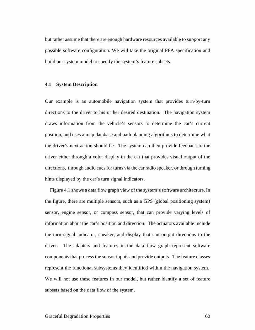
but rather assume that there are enough hardware resources available to support any

possible software configuration. We will take the original PFA specification and

build our system model to specify the system’s feature subsets.

4.1 System Description

Our example is an automobile navigation system that provides turn-by-turn

directions to the driver to his or her desired destination. The navigation system

draws information from the vehicle’s sensors to determine the car’s current

position, and uses a map database and path planning algorithms to determine what

the driver’s next action should be. The system can then provide feedback to the

driver either through a color display in the car that provides visual output of the

directions, through audio cues for turns via the car radio speaker, or through turning

hints displayed by the car’s turn signal indicators.

Figure 4.1 shows a data flow graph view of the system’s software architecture. In

the figure, there are multiple sensors, such as a GPS (global positioning system)

sensor, engine sensor, or compass sensor, that can provide varying levels of

information about the car’s position and direction. The actuators available include

the turn signal indicator, speaker, and display that can output directions to the

driver. The adapters and features in the data flow graph represent software

components that process the sensor inputs and provide outputs. The feature classes

represent the functional subsystems they identified within the navigation system.

We will not use these features in our model, but rather identify a set of feature

subsets based on the data flow of the system.



Figure 4.1. PFA Graph of the Navigation System from [Nace2002] (Used WithPermission).

4.2 Specification of the System Utility Function

Since the system architecture is expressed as a data flow diagram, we can directly

apply our system model and identify feature subsets. The data elements in Figure

4.1 will become our system variable definitions. We identified 22 system variables

that are directly generated from the data elements described in the PFA graph (all

system variable names are in italics): AvgWheelSpeed, Acceleration, ThrottleAngle,

SteeringAngle, YawRate, GroundSpeed, CurrentDirection, CurrentLocationRaw,

CurrentLocation, MapDataRaw, MapData, UpdateMap, DesiredDestination,

PathInfo, TurnInfo, TurnSound, TurnText, SpeakerCommands,

TurnSignalCommands, MapDrawCommands, MapImage, and DisplayMap. Note

that we combined the current location and error estimate data elements into the

single CurrentLocation system variable, since the error estimate can be

implemented as an attribute of the location data. The sensors, actuators, adapters,

and features will become our system components. There are 9 sensors, 3 actuators,

and 33 software components for a total of 45 system components. Without our

model this would require manually evaluating the relative utility of 245 ≈ 4 * 1013

system configurations. If we eliminate all of the invalid system configurations,

there are approximately 6 * 1011 valid possible configurations for which we still

must specify relative system utility values.

We will apply our system model to the data flow graph starting at the system

actuators and working backwards to generate the system’s feature subsets. At the

system level, there are three functional capabilities (Turn Signal, Speaker, Display)

derived from the three actuators available in the system that provide user

functionality. The driver will receive navigation information as long as at least one


of these three capabilities provides positive utility. Figure 4.2 shows the top level

functional capabilities and the feature subsets of which they are composed. The

Turn Signal and Speaker capabilities each contain one feature subset, while the

Display capability has eight feature subsets that can provide display functionality.

Figures 4.3 and 4.4 show definitions of the feature subsets which are

encapsulated by the system-level capabilities. Figure 4.3 details the hierarchical

feature subset definitions for the Turn Signal and Speaker feature subsets. Figure

4.4 defines the feature subsets from two of the eight available Display feature

subsets. Based on the feature subset dependencies, we can see that for the system to

provide any utility in a given configuration, that configuration must contain enough

components for working Location and Map Data feature subsets. The Turn Signal

and Speaker feature subsets depend on the TurnInfo feature subset, which in turn

depends on the Path Planner and Location feature subsets. The Path Planner feature

subset then also depends on the Location and Map Data feature subsets. Each of the

eight possible Display feature subsets depends on at least a working Location and

MapData feature subset.


Display Capability Turn Signal Capability

Display01 Display02 Display03 Display04


Turn SignalFeature Subset

Speaker Capability

SpeakerFeature Subset

Figure 4.2. System-Level Functional Capabilities.

Since the system functionality heavily depends on providing valid location data,

it is not surprising that the designers focused their efforts on providing several levels

of heterogeneous redundancy for this subsystem. Figure 4.5 shows the Location

feature subset in detail. In addition to using the GPS sensor to get accurate location

data, the system has several dead reckoning algorithms available in the event that

GPS location data is lost. Similarly, the dead reckoning algorithms require both


Map DataFeature Subset

MapDataCurrentLocation

LocationFeature Subset

PathInfo

Path PlannerFeature Subset

UserInterface

Destination

TurnInfo

Text

TurnSound

TurnInfoCvt2

TurnInfoCvt

SpeechSynth

SpeechSynthSimple

Speaker


TurnInfoFeature Subset

TurnSpeakerDriver Speaker

Commands

TurnInfo

Turn SignalIndicator


TurnInfoFeatureSubset

TurnSignalDriver

TurnSignalCommands

CurrentLocationTurnInfo

Gen1


LocationFeature Subset Path Planner

Feature Subset

TurnInfo

PathInfo

TurnInfoGen2

TurnInfoGen3

TurnInfoGen4

TurnSound

SoundCommandFeature Subset



Actuator

Feature Subset BoundaryWeak DependenceStrong Dependence

PathPlanner

Figure 4.3. Expansion of Turn Signal and Speaker Feature Subsets.

speed and location data, which can be derived from multiple sensors within the car

with a bit of data transformation. The graceful degradation of the location

subsystem manifests in the loss of accuracy in the location data provided when the

high accuracy components fail. This may reduce the effectiveness of the system’s

path planning navigation algorithms, making the directions that are provided to the

user through the system actuators less accurate.

We were able to completely specify the navigation system with 24 feature

subsets, the largest of which had 6 components, and 3 functional capabilities that

encompass all feature subsets. This means there is an upper bound of 24 * 26 = 1536

feature subset configurations that must be evaluated to specify the utility functions

for all feature subsets. However, this assumes that all feature subsets have the

maximum 6 components, and that all feature subset configurations are valid. We


Display

RenderMapFeature Subset

Map04DisplayMap

MapImage

Display04Feature Subset


MapDataFeature Subset

RenderMap

MapImage

MapData


PathPlannerFeature Subset

PathInfo

CurrentLocation

Display

RenderMap2Feature Subset

Map08DisplayMap




RenderMap2

MapDrawCommands

MapData



PathInfo

CurrentLocation

MapDrawCommands

CurrentLocation

MapDataServer

LocationSentry

Map DVD


MapDataRaw

UpdateMap

MapData



Actuator

Feature Subset BoundaryStrong Dependence

Figure 4.4. Partial Expansion of Display Feature Subsets.

were able to eliminate many invalid feature subset configurations based on

component dependencies. The total number of feature subset configurations we had

to specify was 106.

If we look at the capability configurations there is one valid feature subset

configuration for both the Turn Signal and Speaker capabilities, and 28 - 1 = 255

valid configurations for the Display capability that has eight feature subsets.

Although the Display capability has 255 valid configurations, we will not have to

specify their utility values individually. Since there is only one Display actuator it

can only receive inputs from one of the eight map components at a time to provide


CurrentDirectionBestDead

Reckoner

GPS NullReckoner

SpeedFeature Subset

CurrentLocation

DirectionFeature Subset

GroundSpeed

BetterDead

Reckoner

GoodDead

Reckoner

SimpleDead

Reckoner

GPS1

CurrentLocationRaw


ThrottleAngle

CvtWheelSpeed

SpeedFeature Subset GroundSpeed

SpeedIntegrator1 Speed

Integrator2

GPS1

VDC MM1 EngineSensor

AccelerationAvgWheelSpeed

YawRate

YawGenerator


CurrentDirection

DirIntegrator

GPS1

LWS MM1SboxSteering

Angle

Compass

Dead ReckoningFeature Subset


CurrentLocation

VDCSpeedFeature Subset

MM1SpeedFeature Subset

EngineSpeedEstFeature Subset

GroundSpeed GroundSpeed GroundSpeed




YawRate

Yaw RateFeature Subset




Figure 4.5. Expansion of the Location Feature Subset.

utility. Therefore, we only need to rank the relative utility of the 8 Map feature

subsets to specify the utility of the Display capability. When multiple feature

subsets are available in the system configuration, the Display will only use the one

that provides the most utility. The other feature subsets are treated as backups.

Since we need at least one working capability to provide positive system utility,

there are 23 -1 = 7 possible configurations at the system level that must be specified

to complete the system utility function. We have a total of 123 configurations that

must be specified (106 in feature subsets, 10 in functional capabilities, 7 system

capability configurations) to evaluate the relative utility for all 6 * 1011 valid system

configurations. Appendix B contains all of the feature subset definitions along with

our utility specification.


4.3 Mechanisms that Contribute to Graceful Degradation

Since this example system was designed to provide a high level of graceful

degradation, we can perceive characteristics of the architecture through our system

model that seem to particularly enhance the system’s ability to gracefully degrade.

Several aspects of this system’s software architecture stand out:

• The architecture has well-defined interfaces among components that

provide for logical partitioning of the system into subsystems.

• Subsystems that provide required functionality are targeted for an increased

level of functional redundancy and brute-force redundancy.

• Heterogeneous redundancy is available to provide multiple alternatives for

providing system outputs and completing system requirements.

• Subsystems are designed to be robust to input failures so that they can

continue to provide utility when system variable inputs are not available.

We will examine each of these aspects in both the navigation system and the

brake-by-wire system discussed in the previous chapter to derive a set of heuristics

that should help improve graceful degradation for distributed embedded systems.

4.3.1 Well-Defined System Component Interfaces

In order for a system to provide graceful degradation, the individual subsystems

should be decoupled so that they can tolerate failures from other parts of the system.

One method of decoupling subsystems is to define a set of system interfaces that

restrict the amount of state that is passed among components. In distributed

embedded systems, these interfaces should map to a set of system state variables


that represent the key data elements that are required across different subsystems.

In our system model the interfaces are represented by the set of defined system

variables. Since the system components and subsystems are only coupled through

system variables, making individual subsystems and components robust to losses of

inputs should improve the system’s ability to gracefully degrade.

Unfortunately, producing well-designed component interfaces is a fundamental

problem of software and system architecture. One of the key insights of software

architecture is that the interfaces among components can have as much of an impact

on the system as the components themselves. The software architecture view of

components and connectors emphasizes specifying the connectors in as much detail

as the components.

Within the context of distributed embedded systems, we reduce the general

interface problem to only specifying what data will be passed in the system state

variables. System designers must have domain knowledge so that they can identify

what internal transformations are useful from sensor data values to actuator

command values. If we are dealing with a real-time control system, we can use the

control system parameters as a starting point for identifying system variables.

The system variables should provide logical partitioning of the system into

subsystems, as well as computational “checkpoints” that represent intermediate

steps in the system’s processing. For example, in the automobile navigation system,

two of the major system variables are the CurrentLocation and MapData variables.

Every part of the system that provides functionality depends on receiving these two

data variables. The PathPlanner component requires their data values to provide an

accurate path to the destination. All of the Map components that output to the


Display actuator must have access to map and location information to give the

driver any information about where the car is traveling. However, the PathPlanner

and Map components do not require the CurrentDirection and GroundSpeed

variables that were used to calculate the CurrentLocation variable in some

instances. Thus, in order to ensure that the system gracefully degrades, we can

either provide multiple sources for these data elements, or design components that

require them as inputs to tolerate their loss.

We can use our system model to recognize whether a system’s interface is more

or less conducive to providing graceful degradation. Since feature subsets are

defined based on component interfaces, in general, the number of feature subsets

will scale with the number of defined system variables. If the interface has many

system variables, there will be many feature subsets defined in the system relative to

the number of components in each feature subset (p >> k), and we will have to

consider building mechanisms into each one to tolerate input failures. This may be

cost-prohibitive if a large fraction of these feature subsets are required to provide

any system utility. However, if the interface has few system variables, there will be

few feature subsets defined relative to the number of components in each feature

subset (p << k). This would seem to indicate that feature subsets are large,

monolithic, and complex. Then, using brute-force redundancy to completely

replicate these feature subsets would seem to be the best way to achieve graceful

degradation. Unfortunately this would also be expensive in terms of system

resources. There should be a “sweet spot” in which the number of system variables

and feature subsets are within an order of magnitude of the number of components

per feature subset, where the graceful degradation techniques we propose at the


subsystem level should have the maximum effect for the least system design effort

and resource cost.

Beyond understanding the system’s problem domain and applying the traditional

approach of modular system decomposition, we do not have any new insight on how

to design system interfaces that are ideal for graceful degradation. For this research,

we have focused on developing techniques that will be scalable given that the

system component interfaces are designed so that we have well-partitioned logical

subsystems. Since this is already a goal for well-designed system architectures, and

we have reduced the scope to defining state variables in distributed embedded

systems, this should be a reasonable assumption.

4.3.2 Targeted Redundancy for Critical Subsystems

As a general graceful degradation approach, this mechanism is similar to the

simplex architecture [Bodson93]. We build a subsystem with multiple functionally

redundant software components that provide tradeoffs between their complexity

and the accuracy of their outputs. The simpler components should be less prone to

failures, but will not provide as much utility as the more complex components. We

could also add brute-force hardware redundancy for subsystems that are identified

as single points of failure. It may be more feasible to apply brute-force redundancy

such as replicated system resources to only those parts of the system that are

identified as mission-critical, rather than replicating all of the system’s components.

The best example for this type of redundancy in the navigation system is the

Location feature subset. The location data is critical for the system’s ability to


provide its navigation functionality. Therefore, the location subsystem must be

especially resilient to component failures. However, implementing redundant

backup systems with complete functionality may be cost-prohibitive. For example,

the GPS sensor and software may be an expensive set of components to replicate.

The dead reckoner subsystem provides functional redundancy to the GPS sensor,

with a tradeoff of reduced accuracy of location data. Similarly, the TurnInfo feature

subset contains multiple software components that may have different algorithms

for providing real-time turn information to be communicated to the driver through

the turn signal indicator and speaker.

In the brake-by-wire system, discussed in Chapter 3, the Brake Pedal and

Anti-Lock feature subsets represent critical redundant functionality that trades

accuracy and performance for dependability. Each brake controller has direct

access to the data from the brake pedal controller in the event that the anti-lock

braking subsystems for each wheel fail. With this data, the system can still provide

low-performance braking functionality. Additionally, the Brake Pedal feature

subset is replicated in hardware since it can be a single point of failure in the system

and requires high reliability.

4.3.3 Heterogeneous Redundancy

We define heterogeneous redundancy as subsystems that are designed to provide

different functionality when the system is operating normally, but can be used as

redundant backups at reduced utility when failures occur. Heterogeneous

redundancy is similar to analytic redundancy but is broader in scope.


Heterogeneous redundancy covers not only components and subsystems that are

considered functionally equivalent, but also subsystems that may satisfy the same

requirements with different functionality.

Heterogeneous redundancy can take many forms. There may be several sensors

available in the system that monitor different aspects of the environment that are

physically related, such that one sensor’s data can be synthesized by applying a

transform function to another sensor’s data. For example, if a system has sensors

that monitor temperature, pressure, and volume of a gas, a software component can

be designed to implement a transform function to synthesize the output of one

sensor based on the readings of the other two. Thus, one sensor failure could be

tolerated with this transformer component, without having to add redundant

sensors. Another example of heterogeneous redundancy would be multiple sensors

that have varying degrees of accuracy, such as the GPS speed sensor versus the

wheel speed sensor in the navigation system. Both sensors may output essentially

the same data, but in different formats that must be translated to a system variable

interface. One sensor may provide more utility because its data is more accurate and

reliable, but the other sensor can provide a redundant backup.

In the automobile navigation system, heterogeneous functionality is available at

the system level. The main requirement of the system is to provide navigation aid to

the driver by giving turn-by-turn real-time directions. The system has three distinct

actuators that can provide system utility: the turn signal lights on the dash board, the

car’s radio speaker, and the visual display installed in the car with the navigation

system. In general, we would expect the visual display to provide the most utility

and give the driver the most information about the driving route. However, if the


display suffers a failure, the system can still provide utility via the turn signal lights

and audio cues from the speaker. The failure of any of these three functions is

compensated by the availability of navigation information from the other two

actuators, even though they are not designed to provide the same or equivalent

functionality. This redundancy is a consequence of the functionality built into the

system.

In the brake-by-wire system, there is heterogeneous redundancy by virtue of the

fact that there is one braking subsystem for each of the four wheels in the car.

During normal operation, each of the four brake actuators applies braking force to a

separate wheel to stop the car. However, if one of the actuators failed, the car would

still be able to brake, perhaps with an increased stopping distance. Even if three of

the four brake actuators failed, one working brake actuator would still be useful in

helping the driver regain control of the car.

4.3.4 Component Robustness to Loss of Inputs

Designing individual components (and feature subsets) to be robust to input failures

complements designing subsystems to provide redundant sources of output system

variables. If a component can tolerate the loss of a system variable when all of its

input sources have failed, it may still provide reduced utility and prevent a system

failure. This may not be possible in all situations, but we can identify some

guidelines that might help implement this design approach. Within our system

model, this would be represented by transforming arrows in the data flow graph that


represent strong dependence on system variable inputs, to arrows that represent

weak dependance or treat system variable inputs as optional.

One approach that can make components robust to a loss of input failures is to

design a component with multiple algorithms that provide similar functionality with

each possible combination of required inputs. Of course this will add a great deal of

complexity to the component, as it must manage multiple algorithms as well as

transition between algorithms when inputs are lost. Within a feature subset, these

algorithms may be separated into multiple components, as with the Map feature

subsets defined in the Display capability in the navigation system.

Another approach might be to initially specify the component’s output to provide

some “base level” utility with a minimum of system variable inputs and a default

behavior. Then any other inputs that are available should be treated by the

component as “advice” that modifies the default behavior in specific ways. For

example, if the brake controllers in the brake-by-wire system lost both the brake

pedal and anti-lock braking data from those subsystems, they could provide a

default behavior that applies enough pressure to the brakes to hamper the car’s

acceleration, and then will cause the car to come to a gradual stop when the

accelerator is released. This crippled functionality would signal to the driver that

the car needs to be taken in for repairs, while providing at least a low level of

transportation ability. This technique assumes that received inputs will not be

erroneous, which is reasonable because of our fail-fast, fail-silent fault model.

In the navigation system, this technique is not readily visible in the system

architecture. The designers originally intended reconfiguration to be the main

mechanism of graceful degradation, so that when a component that provides


functionality no longer had enough system inputs available, the reconfiguration

manager would swap that component for another that required fewer inputs.

However, it may not be feasible to require a reconfiguration action every time a

component failure occurs, and it might be necessary for some components to be

designed to continue operating even when all input data sources are lost. This is a

defensive strategy for component design to guard against the event that multiple

failures may occur that cause the complete loss of a system variable input.

4.4 Model Analysis and Graceful Degradation Implementation

The techniques described in section 4.3 focus on mechanisms that should increase

the number of valid configurations within individual feature subsets. They

contribute to graceful degradation because reducing the proportion of feature subset

configurations that provide zero utility in general will translate to fewer system

configurations that provide zero system utility. However, it is not feasible to simply

apply all of these graceful degradation techniques to every feature subset in the

system. Each technique has a cost in terms of increased design effort or additional

system resources.

We can use our system model to analyze the system architecture to target which

components and feature subsets should receive graceful degradation support. There

are several properties in the architecture that can be used as indicators for which

parts of the system should be improved with graceful degradation. For example,

with our scalable system utility function generated from the system model, we can

evaluate every configuration in which a single component or feature subset is not


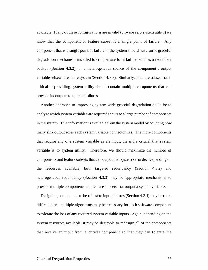
available. If any of these configurations are invalid (provide zero system utility) we

know that the component or feature subset is a single point of failure. Any

component that is a single point of failure in the system should have some graceful

degradation mechanism installed to compensate for a failure, such as a redundant

backup (Section 4.3.2), or a heterogeneous source of the component’s output

variables elsewhere in the system (Section 4.3.3). Similarly, a feature subset that is

critical to providing system utility should contain multiple components that can

provide its outputs to tolerate failures.

Another approach to improving system-wide graceful degradation could be to

analyze which system variables are required inputs to a large number of components

in the system. This information is available from the system model by counting how

many sink output roles each system variable connector has. The more components

that require any one system variable as an input, the more critical that system

variable is to system utility. Therefore, we should maximize the number of

components and feature subsets that can output that system variable. Depending on

the resources available, both targeted redundancy (Section 4.3.2) and

heterogeneous redundancy (Section 4.3.3) may be appropriate mechanisms to

provide multiple components and feature subsets that output a system variable.

Designing components to be robust to input failures (Section 4.3.4) may be more

difficult since multiple algorithms may be necessary for each software component

to tolerate the loss of any required system variable inputs. Again, depending on the

system resources available, it may be desirable to redesign all of the components

that receive an input from a critical component so that they can tolerate the


component’s failure, rather than add redundant backup resources to the component.

This effectively renders the component no longer a single point of failure.

The model analysis provides information about which feature subsets and

components are critical to system utility, allowing us to target these parts of the

system for graceful degradation mechanisms. Choosing which techniques to

implement requires an analysis of the tradeoffs between the resources available in

the system and the level of dependability required. Our scalable specification

framework should enable these tradeoffs to be explicitly identified with the utility

model and information about the resources required for system components and

feature subsets.

In addition to using the model at design time to determine where graceful

degradation mechanisms should be applied in the system, the model can also be

used to validate whether or not the system implementation achieves the level of


0

0.1

0.2

0.3

0.4

0.5

0.6

0.7

0.8

0.9

1

0 0.1 0.2 0.3 0.4 0.5 0.6 0.7 0.8 0.9 1

Predicted Model Utility

Invalid Configurations(Zero Utility)

Configuration withno failed components

(Maximum Utility)

Figure 4.6. Graph of Ideal Case of Predicted Model Utility vs. Measured System Utility.

graceful degradation predicted. In an ideal case the utility model should perfectly

reflect each component and feature subset’s contribution to system utility. If we

have a utility metric that incorporates all of the desired system properties defined in

the system’s requirements, and these attributes can be measured in the system

implementation, then every system configuration’s actual measured utility should

equal the utility predicted by the model. If we graph each configuration’s utility

from the model versus its measured utility for all 2N configurations, we should have

a straight line with a slope of 1 as shown in Figure 4.6.

Unfortunately, in general this ideal case is not possible. Many system properties

such as usability, maintainability, and dependability cannot be readily quantified,

and it is nontrivial to combine these properties along with system functionality and

performance into a single utility metric. Additionally, the utility function generated

in the system model is based on the feature subset definitions and the assumption

that each feature subset’s utility can be evaluated independently for each

configuration. Individual feature subset configuration utility functions may be

based on the designer’s domain knowledge and understanding of the components in

the system. This may lead to a less accurate system utility function that does not

capture all of the interactions between components in the system.

Rather than focus on absolute utility measurements that may be inaccurate, we

can use the relative utility values of system configurations to rank all 2N

configurations in order by increasing utility according to the model. Then we may

select a system property or set of properties such as performance and reliability that

may be measurable for the system implementation, and use this measurement as a

proxy for a system utility metric. If we graph the system configurations by


comparing their utility value as predicted by the model and their system property

metric that is a substitute for a system utility measurement, we expect a graph that

may not be linear, but will be monotonically increasing such that configurations

with higher utility values in the model will have higher system property

measurements. If there are configurations that do not fit the curve in this graph (e.g.

configurations ranked as low utility that have unusually high measured system

properties or configurations ranked as high utility that have low measured system

properties), they may indicate either an inaccuracy in the system model, a

dependability problem in the system implementation, or a violation of the model’s

assumptions (described in section 1.3). We can apply this analysis iteratively to both

refine the system model and identify dependability bottlenecks in the system

implementation.

This analysis assumes that the utility values specified by the system model for all

2N configurations will be accurate enough that in general configurations that

actually have more utility will be ranked higher than configurations that actually

have less utility. It also assumes that the properties selected to measure the system

implementation are indicators of system utility as defined by the system

requirements. The system designer should choose properties for this metric that are

both quantifiable and general indicators of overall system utility. This may be

difficult depending on which properties are considered important by the system

requirements, and whether these properties have tradeoffs with one another. The

current best practice for combining properties into a single utility metric is

multi-attribute utility theory [Keeney76, Keeney 92].


4.5 Summary

In this chapter we have used an example of a complex distributed embedded system

architecture to identify a set of properties that should improve graceful degradation

when applied to a system’s software architecture. Traditional brute-force

redundancy techniques are resource intensive and may not be feasible for

cost-sensitive embedded systems. Therefore we propose some techniques that

apply limited redundancy in terms of both design effort and additional system

resources to parts of the system to improve its ability to gracefully degrade.

We can use our system model for specifying graceful degradation to locate single

points of failure in the system at the component and subsystem level. Then we can

concentrate on adding redundancy to these parts of the system, implementing

multiple subsystems that trade complexity for utility. We can add brute force

hardware redundancy to smaller feature subsets and individual system components

that are mission-critical. We can also identify natural heterogeneous redundancy

that may be already designed into the system, and exploit it for graceful degradation.

Finally, if we adopt a strategy for individual component and subsystem design such

that they are robust to input failures, this will complement the targeted redundancy

that emphasizes providing multiple output sources for system variables.

We also outlined a general analysis technique that uses our system model for

scalable graceful degradation to identify dependability problems in the system

implementation. By measuring relevant system properties of different system

configurations in the implementation and comparing these measurements to the

utility values predicted by the model, we can validate the accuracy of the model.

Any discrepancies between the model prediction and the measurements of the


implementation may be traced to either an inaccuracy in the model or a problem in

the system design and implementation.

The application of the graceful degradation techniques depends on already

having well-defined system variable interfaces that create partitioned feature

subsets. We do not think it is unreasonable to require an architecture that provides

partitioned decoupled subsystems as a prerequisite for providing scalable

system-wide graceful degradation, as this is a fundamental goal of system and

software architecture design. In the next chapters we will demonstrate the

application of these techniques on two representative distributed embedded

systems, and evaluate how they contribute to system-wide graceful degradation.

We also use the analysis methods we have outlined to validate the utility model

compared to an approximate utility measure of the system implementation for each

case study.


5 Case Study: Elevator Control System

To il lus trate how we can ap ply our sys tem model and graceful degradation

techniques to a realistic distributed embedded sys tem, we use a design of a

rel a tively com plex dis trib uted el e va tor con trol sys tem. This sys tem was de signed

by an el e va tor en gi neer (my thesis advisor) and has been im ple mented in a dis crete

event sim u la tor writ ten in Java. This el e va tor sys tem has been used as the course

pro ject in the dis trib uted em bed ded sys tems class at Car ne gie Mellon Uni ver sity for

sev eral se mes ters. Since we have a com plete ar chi tec tural spec i fi ca tion as well as

an im ple men ta tion, we can di rectly ob serve how prop er ties of the system

ar chi tec ture af fect the sys tem’s abil ity to grace fully de grade by per form ing fault

in jec tion ex per i ments in the sim u la tion.

The architectural specification is in the form of a requirements document that

specifies each system component’s inputs and outputs, as well as their functional

behavior. The component interfaces are specified as a message dictionary that

represents all network messages that can be sent among components. We first

describe the elevator system interface in detail, and then apply the graceful

degradation techniques from Chapter 4 to the system architecture. We then apply

our system model to the architecture to specify its ability to gracefully degrade.

Finally, we run a set of experiments on the elevator system using both the original

system architecture and the new architecture with our graceful degradation

improvements. We fail several combinations of components and observe the effect

on the system’s ability to deliver passengers.

Elevator Case Study 83

5.1 Elevator System Architecture

Our view of the el e va tor sys tem is a set of sen sors, ac tu a tors and soft ware

com po nents that are al lo cated to the var i ous hard ware nodes in the dis trib uted

sys tem. The nodes are con nected by a real-time fault-tolerant broad cast net work.

All net work mes sages can be re ceived by any node in the sys tem. Since all

com mu ni ca tion among com po nents is via this broad cast net work, all com po nent

com mu ni ca tion in ter faces map to a set of net work mes sage types.

Our el e va tor sys tem ar chi tec ture is highly dis trib uted and de cen tral ized, and is

based on the mes sage in ter faces that sys tem com po nents use to com mu ni cate.

Sys tem in puts come from “smart” sen sors that have a pro cess ing node em bed ded in

the sens ing de vice. These sen sors con vert their raw sen sor val ues to mes sages that

are broad cast on the net work. The soft ware con trol sys tem, im ple mented as a set of

dis trib uted soft ware com po nents, re ceives these mes sages and pro duces out put

mes sages that pro vide com mands to the ac tu a tors that pro vide the sys tem’s

func tion al ity.

The el e va tor con sists of a sin gle car in a hoistway with ac cess to a set num ber of

floors f. The car has two in de pend ent left and right doors and door mo tors, a drive

that can ac cel er ate the car to two speeds (fast and slow) in the hoistway, an

emer gency stop brake for safety, and var i ous but tons and lights for de ter min ing

pas sen ger re quests and pro vid ing feed back. Since the sen sors and ac tu a tors map

di rectly to the mes sage in ter faces among com po nents, we list all the pos si ble

in ter face mes sage types along with their send ers and re ceiv ers be low to de fine the

com po nents and in ter faces of the sys tem ar chi tec ture. In the fol low ing no ta tion, the

val ues within the “[ ]” brack ets rep re sent the stan dard rep li ca tion of an ar ray of


sen sors or ac tu a tors, and the val ues within the “( )” pa ren the ses rep re sent the val ues

the sen sor or ac tu a tor can out put. For ex am ple, the Hall Call mes sage type maps to

an ar ray of sen sors for the up and down but tons on each floor out side the el e va tor

that is f (the num ber of floors the el e va tor ser vices) by d (the di rec tion of the but ton;

Up or Down) wide, and each but ton sen sor can ei ther have a value v of True

(pressed) or False (not pressed). Un less oth er wise noted, “f” rep re sents the num ber

of floors the el e va tor ser vices, “d” rep re sents a vari able that in di cates a di rec tion of

ei ther Up or Down, “j” is a vari able that is a value of ei ther Left or Right (for the left

and right el e va tor doors), and “v” de notes a value that can be ei ther True or False.

The sen sor mes sage types avail able in the sys tem in clude:

• AtFloor[f](v): Out put of AtFloor sen sors that sense when the car is near a

floor.

• CarCall[f](v): Out put of car call but ton sen sors lo cated in the car.

• CarLevelPosition(x): Out put of car po si tion sen sor that tracks where the

car is in the hoistway. x = {distance value from bot tom of hoistway in

millimeters}

• CarWeight(w): Output of car weight sensor that measures the aggregate

weight of all passengers in the car. w = { weight in car in pounds }

• DoorClosed[j](v): Out put of door closed sen sors that will be True when

the door is fully closed.

• DoorOpen[j](v): Out put of door open sen sors that will be True when the

door is fully open.

• DoorReversal[j](v): Out put of door re ver sal sen sors that will be True

when door senses an ob struc tion in the door way.


• HallCall[f,d](v): Out put of hall call but ton sen sors that are lo cated in

hall way out side the el e va tor on each floor. Note that there are a to tal of 2f -

2 rather than 2f hall call but tons since the top floor only has a down but ton

and the bot tom floor only has an up but ton.

• HoistwayLimit[d](v): Out put of safety limit sen sors in the hoistway that

will be True when the car has over run ei ther the top or bot tom hoistway

lim its.

• DriveSpeed(s,d): Out put of the main drive speed sen sor. s = {speed value},

d = {Up, Down, Stop}

The ac tu a tor com mand messages avail able in the sys tem are:

• DesiredFloor(f, d): Com mand from the el e va tor dis patcher al go rithm

indicating the next floor des ti na tion. d = {Up, Down, Stop} (This is not an

ac tu a tor in put, but rather an in ter nal vari able in the con trol sys tem sent

from the dis patcher to the drive controller)

• DesiredDwell(n): Command from the elevator dispatcher algorithm to the

door controllers indicating how long the doors should remain open when

stopped on a floor. n = { Integer dwell time in milliseconds } (This is also

not an actuator input, but an internal control system variable that allows the

dispatcher to affect the operation of the door motors)

• DoorMotor[j](m): Door mo tor com mands for each door. m = {Open,

Close, Stop}

• Drive(s, d): Com mands for 2-speed main el e va tor drive. s = {Fast, Slow,

Stop}, d = {Up, Down, Stop}


• CarLantern[d](v): Com mands to con trol the car lan tern lights; Up/Down

lights on the car doorframe used by pas sen gers to de ter mine the el e va tor’s

cur rent trav el ing di rec tion.

• CarLight[f](v): Com mands to con trol the car call but ton lights in side the

car call but tons to in di cate when a floor has been se lected.

• CarPositionIndicator(f): Com mands for po si tion in di ca tor light in the car

that tells us ers what floor the car is ap proach ing.

• HallLight[f,d](v): Com mands for hall call but ton lights in side the hall call

but tons to in di cate when pas sen gers want the el e va tor on a cer tain floor.

• EmergencyBrake(v): Emer gency stop brake ac ti vated when ever the

sys tem state be comes un safe and the el e va tor must be shut down to pre vent

a cat a strophic failure.

For each ac tu a tor, there is a soft ware con trol ler ob ject that pro duces the

com mands for that ac tu a tor. The drive con trol ler com mands the drive ac tu a tor to

move the el e va tor based on the DesiredFloor in put it re ceives from the dis patcher

soft ware ob ject. The left and right door con trol lers op er ate their re spec tive door

mo tors. The safety mon i tor soft ware mon i tors the el e va tor sys tem sen sors to en sure

safe op er a tion and ac ti vate the emer gency brake when nec es sary. The var i ous

soft ware ob jects for the but tons and lights de ter mine when to ac ti vate the lights to

in di cate ap pro pri ate feed back to the pas sen gers. The el e va tor con trol sys tem

con sists of 9 + 4f sen sors, 5 + 3f ac tu a tors, and 6 + 3f soft ware com po nents, for a

to tal of 20 + 10f com po nents in the sys tem. Fig ure 5.1 il lus trates how these sys tem

com po nents are al lo cated to hard ware nodes in the el e va tor’s dis trib uted con trol

sys tem. Each software component has a set of inputs and outputs that are specified


from the message interface. Appendix C describes the interface specification for

each of these software components. All components are designed to require all of

their inputs to provide their functionality.

This elevator system is decomposed into several distinct subsystems that have

control over different parts of the elevator system. Although the elevator has

well-defined component and interface definitions, this system was not particularly

designed for graceful degradation. Many of the subsystems are tightly coupled

because they depend on each others’ outputs. For example, the drive controller will

not move the elevator unless it receives commands from the dispatcher, and the

dispatcher cannot effectively service all floors without receiving inputs from all of

the elevator hall call and car call buttons. In the next section we will apply some of

the mechanisms we identified in Chapter 4 to this elevator architecture to give the

system the ability to gracefully degrade.


Fault TolerantBroadcast Network

Safety MonitorController and

Emergency BrakeDrive Motor and

Controller

Drive SpeedSensor

{Left, Right} DoorMotors andControllers

Car PositionIndicator Controller

and Lights

{Left, Right}Door Closed

SensorsCar Position

Sensor

{Left, Right}Door Open

Sensors

{Left, Right}Door Reversal

Sensors

{Up, Down}Hoistway Limit

Sensors

{Up, Down}Lantern Controllers

and Lights

{1 … f} Hall Call{Up, Down}

Button Sensors, Controllers, and Lights

{1 … f} Car CallButton Sensors,,

Controllers, and Lights

DispatcherController

Car WeightSensor

{1 … f} AtFloorSensors


Actuator

Hardware Node

Network Connection

Figure 5.1. Hardware View of Elevator Control System.

5.2 Adding Graceful Degradation to the Elevator System

In order to apply the graceful degradation techniques we identified, we first

examined which parts of the system should be considered mission-critical, and

which could be considered functional enhancements that can be lost without

causing a system failure. An elevator system’s most basic requirements are that it

protect passenger safety while using the system and transport passengers to their

destination floors without stranding them or trapping them in the elevator. Other

services typically associated with an elevator system, such as providing appropriate

passenger feedback and efficiently processing passenger requests, can be

considered “optional” functionality. As long as the elevator maintains passenger

safety, and can (eventually) service all floors, the elevator can still be considered

“working.”

Based on the software components defined for this elevator system, the safety,

drive control, and door control subsystems are responsible for satisfying the basic

elevator requirements. Therefore, we can significantly improve the system’s ability

to gracefully degrade if we can ensure that these subsystems can tolerate failures

from all other parts of the system. We can achieve this by redesigning system

components to tolerate multiple input failures, and by adding redundant

components to critical subsystems.

The safety monitor component requires all of its sensor inputs to keep track of the

elevator’s state and ensure that the elevator does not violate its safety conditions. If

a violation is detected, the safety monitor will trigger the emergency brake and will

cause a complete shutdown of the elevator system. Therefore we are unlikely to find

any graceful degradation opportunities in the safety subsystem, as all of the


components are required to prevent a catastrophic system failure that may harm the

passengers. A loss of any of the sensor inputs by the safety monitor will by design

trigger an emergency shut down.

There are several modifications we can make to the drive controller that will

make it robust to input failures, which is one of the graceful degradation strategies

we propose in Section 4.3.4. The drive controller depends on the dispatcher to

provide commands that tell the drive where to move the elevator in the hoistway, but

we can redesign the drive controller component to tolerate the loss of the dispatcher

input. If we design the drive to have a default behavior such that it will periodically

visit every floor when the input from the dispatcher is not available, this will

guarantee that the drive controller can continue to provide elevator service if the

dispatcher fails. When the dispatcher is working and providing inputs to the drive

controller, the drive controller lets the dispatcher command override its default

behavior.

The drive controller also uses the floor, drive speed, and car position sensors to

determine what commands to send to the drive motor to travel in the hoistway. At

the drive motor’s slow speed, the elevator only needs floor sensor data to reliably

stop level with a floor. In order to travel faster in the hoistway, the drive controller

uses the car position sensor to calculate the appropriate stopping distance to

determine when to decelerate from fast to slow before approaching a destination

floor. We can ensure that the drive controller will tolerate car position sensor

failures by designing it to only command the drive motor to fast if the car position

sensor’s input is available, and to immediately command the drive motor only to


slow if the car position sensor data is lost. This will significantly impact elevator

performance, but will continue to guarantee basic elevator requirements.

We can also redesign the dispatcher component to be robust to hall call and car

call button failures. The dispatcher implements an algorithm to efficiently process

passenger requests by listening to these button inputs. If a button for a particular

floor fails, we do not have to change the algorithm, but can simply synthesize an

internal request for that floor periodically that will be incorporated into the

dispatcher’s regular algorithm. This will guarantee that the dispatcher does not

“starve” floors on which all of the buttons have failed. This is an extension of our

strategy for heterogeneous redundancy and making components robust to input

failures, described in Sections 4.3.3 and 4.3.4. The dispatcher takes over the

responsibility of generating hall call and car call sensor data internally when some

of these sensors fail. This provides a redundant backup for these sensors in the

context that their floors continue to be periodically processed into the dispatcher

algorithm, even thought their buttons are disabled. This also has the benefit of

making the dispatcher software component robust to input failures.

Ad di tionally, since the AtFloor sen sors are a crit i cal re source for the el e va tor

sys tem (nearly every subsystem requires Atfloor sensor data), we add re dun dant

“vir tual” AtFloor soft ware com po nents that can syn the size AtFloor mes sages based

on data from the car po si tion and el e va tor drive speed sen sors. If some of the

phys i cal AtFloor sen sors fail, these soft ware sen sors can be used as back ups. These

virtual AtFloor sensors implement data transformations to provide backup Atfloor

sensor data and will only transmit their messages when the real Atfloor sensors fail.

This draws on the techniques for targeted and heterogeneous redundancy, described


in Sections 4.3.2 and 4.3.3. The AtFloor sensors are a critical system resource, and

thus a target for additional redundancy to improve system dependability. We can

provide this redundancy by synthesizing AtFloor sensor data from other sensors

already available in the system, rather than having to add additional physical

sensors.

All of the changes made to the implementation to add these graceful degradation

mechanism did not require a large amount of code. Ignoring the simulation code

that was not altered for either system, the objects that implement the elevator control

system in the original design had a total of 1,659 lines of code. The gracefully

degrading system had a total of 1,807 lines of code in the control system

implementation. This is only a 9% increase in code size to implement all of our

modifications for graceful degradation.

Our goal was to identify what changes we could make to the software system to

give the elevator system the ability to gracefully degrade. Thus, although we

identified the critical parts of the system that could benefit from receiving brute

force hardware redundancy, we did not add it to our system. Rather, we evaluated

the system’s ability to gracefully degrade by restricting our component fault

injection only to those parts of the system that were enhanced with graceful

degradation mechanisms. The mission-critical sensors, actuators, and software

components (components that make up the safety, drive control, and door control

subsystems) only represent 25% of the total components in the system. We know

that if we fail parts of the system that provide mission-critical functionality, the

system will fail, but we are interested in ensuring that any failures in the other 75%


of the components in the system will not cause a complete system failure, but rather

will allow the system to gracefully degrade.

5.3 Specifying the Utility Function of the Elevator Control System

We can use the component and interface specifications of the elevator control

system to apply our system model for graceful degradation. We will not reproduce

the entire system data flow graph here, but rather show the subgraphs for each

feature subset we identified and how we performed our analysis using these

subsystem definitions. These feature subsets will be defined based on the system

architecture after we have made the graceful degradation improvements. Many of

these improvements will manifest in the model as data flow arcs between

components that are optional rather than strongly dependent relationships. The

feature subset definitions of the original elevator system architecture would each

have only one valid configuration since each subsystem is dependent on all of its

inputs to provide utility.

There is a significant amount of functional repetition in the elevator system.

There are two door controllers and two sets of door sensors and actuators, but their

only functional difference is that one controls the left door and one controls the right

door. Similarly, all of the car call and hall call button software components are

implemented as objects that are instantiated at run time from one car call class and

one hall call class. However, in the software view of our model, these objects are all

considered distinct components that make up distinct feature subsets. Most of these

sets of components have one instantiation per floor. They cannot be considered


logically equivalent because each component in the set only provides functionality

for a single floor.

These replicated components form nearly identical feature subsets that have

identical sets of valid configurations, and are replicated on a per floor basis. Thus

we can take advantage of this replication to reduce the number of utility

specifications. One utility specification can be applied to the entire set of replicated

feature subsets. This replication does not represent redundancy for fault tolerance

or graceful degradation, but rather is a consequence of distributing functionality for

multiple identical system behaviors. The elevator treats every floor the same, so one

base class can be designed that generates distinct software objects per floor for

similar functionality.

At the system level, there are seven major functional capabilities that provide

utility: the safety monitor, drive control, door control, hall call buttons and feedback

lights, the car call buttons and feedback lights, the car lantern lights, and the car

position indicator lights. These capabilities can each be represented by a single

feature subset that encapsulates other subsystems in the elevator architecture.

These feature subsets are outlined in the following section.

5.3.1 Elevator Feature Subsets

In the el e va tor sys tem, there are sev eral func tional sub sys tems that map to fea ture

sub sets. The pri mary con trol sys tems in the el e va tor op er ate the drive and the door

mo tors. Their fea ture sub sets are de fined by the in puts and out puts of the drive

con trol ler, and left and right door con trol ler soft ware ob jects. Fig ure 5.2 dis plays


these fea ture sub sets and the de pend ency re la tion ships among their com po nents. In

the di a grams we an no tated the out put vari ables of each fea ture sub set. The left and

right door con trol fea ture sub sets are nearly iden ti cal with the ex cep tion of which

door sen sors and ac tu a tors they con tain, so only the left door con trol fea ture sub set

is shown in de tail. Both door control feature subsets can be covered with one utility

specification that is applied separately based on their configurations.

These fea ture sub sets are re spon si ble for con trol ling the drive and door ac tu a tors,

but they also out put their com mand vari ables over the net work to the rest of the

sys tem. This al lows subsystems to loosely co or di nate their op er a tion with out be ing

strongly cou pled and de pend ent on each other. For ex am ple, the Door Con trol lers

must re ceive in puts from the Drive Speed sen sor in or der to safely op er ate the door

only when the el e va tor is not mov ing. How ever, the Door Con trol ler can also use


Right DoorCommand Message

Left DoorControllerLeft Door

Motor

Left DoorOpen

Sensor

Left DoorReversalSensor

Left DoorCommand Message

Door ControlFeature Subset

{Left, Right} DoorCommand Messages

Left DoorControl

Feature Subset

Right DoorControl

Feature Subset

Left DoorClosedSensor

Drive SpeedSensor

DriveControl

AtFloorSensors

Desired FloorSubsystem

Car CallButtons

Hall CallButtonsDrive

Controller

Drive Motor

Door Control

AtFloorSensors

Hoistway LimitSensors

Drive SpeedSensorCar Position

SensorDesired FloorSubsystem

SafetyMonitor

DoorClosed

Sensors

Drive ControlFeature Subset Drive

CommandMessage

Feature Subset BoundarySensorSoftware ComponentFeature Subset

Actuator


Strong Dependence

Figure 5.2. Feature Subset Graphs of the Door and Drive Control Subsystems.

the com mand out put from the Drive Con trol fea ture subset to an tic i pate when the

el e va tor will stop based on the com mand sent from the Drive Con trol fea ture sub set,

thus al low ing more ef fi cient door op er a tion via sending the door open command

slightly be fore the el e va tor is level with the des ti na tion floor. The Drive Con trol

fea ture sub set en cap su lates all of its com po nents, so that it is rep re sented as a sin gle

com po nent that out puts the Drive com mand sys tem vari able in the Left and Right

Door Con trol fea ture sub sets. Like wise the Door Con trol fea ture sub set

en cap su lates all of the com po nents in the Left and Right Door Con trol fea ture

sub sets.

These fea ture sub sets also con tain sev eral iden ti cal com po nents, such as the

Drive Speed and AtFloor sen sors. These com po nents do not rep re sent mul ti ple

cop ies of the same com po nent in the soft ware data flow view, but rather that these

fea ture sub sets over lap and share some of their com po nents. The fea ture sub set

graphs show de pend en cies among com po nents, but not whether in di vid ual

com po nents are rep li cated for mul ti ple sub sys tems. There may be mul ti ple

re dun dant sen sors in stalled in the sys tem, but the in for ma tion about how

com po nents are al lo cated to hard ware would be vis i ble in the hard ware ar chi tec ture

and is or thogo nal to the soft ware data flow view of our sys tem model.

We de fined sev eral other fea ture sub sets for our el e va tor sys tem in ad di tion to the

Door Con trol and Drive Con trol fea ture sub sets. The safety mon i tor soft ware

com po nent and its in puts and out puts de fines the Safety Mon i tor fea ture sub set. The

Safety Mon i tor fea ture sub set is re spon si ble for de tect ing when the el e va tor sys tem

state be comes un safe, such as the doors open ing while the el e va tor is mov ing, the

doors fail ing to re verse di rec tion if they bump into a pas sen ger while clos ing, or the


el e va tor overrunning into the top or bot tom of the hoistway. In any un safe sit u a tion,

the safety mon i tor must trig ger the emer gency brake ac tu a tor that shuts down the

el e va tor sys tem to pre vent a cat a strophic fail ure. Fig ure 5.3 shows the Safety

Mon i tor fea ture sub set along with some of the sen sors from which it re ceives in puts.

The safety mon i tor must re ceive in puts from both the Door and Drive Con trol

fea ture sub sets to en sure that their com mands are con sis tent with the el e va tor’s

ac tual op er a tion de ter mined from the drive speed and door sen sors.

The Door Con trol, Drive Con trol, and Safety Mon i tor fea ture sub sets rep re sent

the crit i cal el e va tor sub sys tems that pro vide an el e va tor’s ba sic func tion al ity. An

ef fi cient el e va tor should also re spond to pas sen ger re quests to move peo ple quickly

to their des ti na tion floors. The Drive Con trol ler lis tens to the DesiredFloor sys tem

vari able to de ter mine its next des ti na tion, and this vari able is the out put of the

De sired Floor fea ture sub set. The De sired Floor fea ture sub set con tains the


Safety MonitorController

EmergencyBrake Actuator

DoorControl

Door ClosedSensors

Door ReversalSensors

Drive SpeedSensor

DriveControl AtFloor

Sensors

HoistwayLimit

Sensors

Safety MonitorFeature Subset

EmergencyBrake

Message

Left DoorClosed

Message

Left DoorClosed Sensor

Right DoorClosed Sensor

Right DoorClosed

Message

{Left, Right}Door ClosedMessages

Left DoorReversalMessage

Left DoorReversal Sensor

Right DoorReversal Sensor

Right DoorReversalMessage

{Left, Right}Door Reversal

Messages

HoistwayLimit UpMessage

Hoistway LimitUp Sensor

Hoistway LimitDown Sensor

HoistwayLimit DownMessage

Hoistway Limit{Up, Down}Messages

Door ClosedSensors

Feature Subset


Feature Subset


Feature Subset



Actuator


Strong Dependence

Figure 5.3. Feature Subset Graphs of the Safety Monitor Subsystem.

dis patcher soft ware com po nent that im ple ments the al go rithm for de ter min ing the

next floor at which the el e va tor should stop. The dispatcher also outputs the

DesiredDwell system variable to the door controllers to control how long they hold

the doors open on a floor.

The dis patcher re ceives in puts from the car call and hall call but tons to de ter mine

pas sen ger in tent and com pute the el e va tor’s next des ti na tion. The dispatcher can

also use the elevator’s weight sensor to determine when the car is full, thus

bypassing hall call requests in favor of car call requests to unload the car. The car

call and hall call but tons in turn form their own fea ture sub sets that pro vide the

but ton sen sor mes sages to the rest of the sys tem, but also con trol the but ton lights to

pro vide ap pro pri ate pas sen ger feed back. Fig ures 5.4 and 5.5 show the fea ture


DispatcherController

AtFloorSensors

Drive SpeedSensor

Door ClosedSensors


Feature SubsetDesired FloorMessage

Car CallButtons

Hall CallButtons

Car Call ButtonsFeature Subset Car Call {Floor 1 … f}

Messages

Car CallFloor 1FeatureSubset

Car CallFloor 2FeatureSubset

Car CallFloor fFeatureSubset

Car CallFloor 1

Message

Car CallFloor 2

Message

Car CallFloor f

Message

…

Car CallFloor 1

Controller

Car CallFloor 1

Message

Car Call LightFloor 1

Command MessageCar Call

Floor 1 ButtonLight

Car CallFloor 1

Button SensorAtFloorFloor 1Sensor

Door ClosedSensors



Actuator


Strong Dependence

Car WeightSensor

Figure 5.4. Feature Subset Graphs for the Desired Floor and Car Call ButtonSubsystems.

sub set def i ni tions for the De sired Floor, Car Call and Hall Call fea ture sub sets. The

fea ture sub sets for the car call and hall call but tons are sim i larly defined for each

floor since each car call and hall call soft ware con trol ler have sim i lar in put and

out put in ter faces and are replicated instances of the same base class. Each car call

and hall call con trol ler out puts the value of its re spec tive sen sor on the net work for

the rest of the sys tem, but only sends the com mand mes sages for its but ton light to

its ac tu a tor.

In or der to en cour age peo ple to move quickly in the el e va tor, the car lan tern and

car po si tion in di ca tor lights pro vide feed back to let the pas sen gers know the

el e va tor’s cur rent trav el ing di rec tion, and the el e va tor’s next floor des ti na tion.


Hall Call UpButtons

Feature Subset

Hall Call Up{Floor 1 … f-1}

Messages

Hall Call UpFloor 1

Feature Subset

Hall Call UpFloor 2

Feature Subset

Hall Call UpFloor f-1

Feature Subset

Hall Call UpFloor 1 Message


Hall Call UpFloor f-1 Message

…

Hall Call UpFloor 1

Controller


Hall Call Up LightFloor 1

Command Message

Hall Call UpFloor 1 Button Light

Hall Call UpFloor 1

Button Sensor

AtFloorFloor 1SensorDoor Closed

Sensors

Hall Call DownButtons

Feature Subset

Hall Call Down{Floor 2 … f}MessagesAll Hall Call

Messages

Hall CallButtonsFeatureSubset




Actuator


Strong Dependence

Figure 5.5. Elevator Hall Call Button Feature Subsets.

Fig ure 5.6 dis plays the fea ture sub sets for the Car Po si tion In di ca tor and Up and

Down Car Lan tern light sub sys tems. These fea tures are not es sen tial for the

el e va tor’s ba sic op er a tion, but pro vide in for ma tion to the pas sen gers to help them

use the el e va tor more ef fi ciently.

One es sen tial sub sys tem that is re quired by all of the other ma jor el e va tor

sub sys tems is the AtFloor Sen sors fea ture sub set. Nearly ev ery fea ture sub set

strongly de pends on AtFloor sen sor in for ma tion to pro vide func tion al ity. For

ex am ple, the Drive Con trol and Door Con trol fea ture sub sets need the AtFloor

sen sor in for ma tion to cor rectly op er ate the drive and door mo tors. Since this is such

a crit i cal fea ture in the el e va tor sys tem, our el e va tor de sign also has re dun dant

soft ware com po nents. The vir tual AtFloor soft ware com po nents can syn the size

AtFloor sen sor mes sages from the car po si tion and drive speed sen sors when the

phys i cal AtFloor sen sors fail. Thus they are in cluded in the AtFloor sen sor fea ture


Car LanternDown LightCommandMessage

Lantern UpControllerCar Lantern

Up Light

Car LanternUp LightMessage

Car LanternFeature Subset Car Lantern

{Up, Down}Command Messages

LanternControl Up

Feature Subset

Lantern ControlDown Feature Subset

AtFloorSensors

Desired FloorSubsystemDoor Closed

Sensors

Car PositionIndicatorController

AtFloorSensors

Drive SpeedSensor

Car Position IndicatorFeature Subset

Car PositionIndicator Command

Message


Car PositionSensor

Car PositionIndicator

Lights

Feature Subset BoundarySensorSoftware ComponentFeature Subset

Actuator


Strong Dependence

Figure 5.6. Car Position Indicator and Car Lantern Feature Subsets.

sub set graphs. Fig ure 5.7 shows the AtFloor fea ture sub set de scrip tion for the

el e va tor sys tem in our model. As with other replicated components, the virtual

AtFloor sensor components are software objects instantiated from the same base

class.

5.3.2 Utility Analysis

The gracefully degrading el e va tor sys tem has a to tal of 20 + 11f sys tem com po nents

(there are an f extra components, representing each of the virtual Atfloor software

components that we added to the system), mean ing there are 220 + 11f pos si ble sys tem

con fig u ra tions. The sys tem can pro vide ba sic func tion al ity if the min i mum

com po nents nec es sary to op er ate the drive mo tor, door mo tors, and main tain safety

are pres ent. Thus these 17 com po nents (drive con trol ler soft ware, drive speed


AtFloor SensorsFeature Subset AtFloor {Floor 1 … f}

Messages

AtFloorFloor 1

Feature Subset

AtFloorFloor 2

Feature Subset AtFloorFloor f

Feature Subset

AtFloorFloor 1

Message

AtFloorFloor 2

Message

AtFloorFloor f

Message

…

Virtual AtFloorFloor 1 Controller

AtFloorFloor 1 Message

AtFloorFloor 1 Sensor

Drive SpeedSensor

Car PositionSensor



Actuator


Strong Dependence

Figure 5.7. AtFloor Subsystem Feature Subset Graph.

sen sor, drive mo tor, left and right door con trol ler com po nents, left and right door

mo tors, all door sen sors, safety mon i tor soft ware, hoistway limit sen sors,

emer gency brake ac tu a tor), in addition to the components required to provide valid

AtFloor feature subsets for each floor, are fixed and must be pres ent in ev ery valid

con fig u ra tion. All other com po nents (such as the but ton lights and sen sors and

pas sen ger feed back lights) can be con sid ered op tional and pres ent in any

con fig u ra tion. There are 2 + 9f op tional com po nents that can have 22 + 9f pos si ble

con fig u ra tions.

Enough com po nents to pro vide work ing AtFloor fea ture sub sets for each floor

must be pres ent as well. There fore, on each floor there must be a work ing AtFloor

sen sor or a work ing virtual AtFloor com po nent with a work ing car po si tion sen sor.

If the car po si tion sen sor breaks, then all AtFloor sen sors must work, assuming the

worst case scenario that the elevator must service at least one passenger on every

floor. Since all the AtFloor sen sors must work in this sit u a tion, they are fixed and

have one con fig u ra tion. How ever, the virtual AtFloor com po nents can ei ther work

or not work since their fail ure will not af fect the avail abil ity of the AtFloor sys tem

vari ables, mak ing 2f valid com bi na tions for the var i ous virtual AtFloor com po nents.

If the car po si tion sen sor works, then one or both AtFloor sen sor and virtual AtFloor

com po nent must work for each floor, so the only in valid com bi na tions are when

both have failed for at least one floor. This means there are 3 valid com bi na tions per

floor, mak ing 3f valid com bi na tions out of the pos si ble 22f. Thus there are 2f + 3f

valid com bi na tions of com po nents in the AtFloor fea ture sub set.

The to tal num ber of pos si ble valid sys tem com po nent con fig u ra tions af ter

elim i nat ing all con fig u ra tions that will al ways have zero util ity is (2f + 3f)(22 + 9f).


We ran our el e va tor simulator tests with seven floors, so this is ap prox i mately 9 *

1022 con fig u ra tions that still must be man u ally ranked. This is a sig nif i cant

re duc tion from the 297 ≈ 2 * 1029 to tal pos si ble sys tem con fig u ra tions, but still

in trac ta ble for spec i fy ing sys tem-wide grace ful deg ra da tion. How ever, we can

ex ploit the struc ture of the sys tem de sign cap tured in the fea ture sub set def i ni tions

to re duce the num ber of con fig u ra tions we must rank to com pletely spec ify the

sys tem util ity func tion.

We have de fined 16 + 4f dis tinct fea ture sub sets in the el e va tor sys tem. If f is

small, the larg est fea ture sub sets are the left and right door con trol fea ture sub sets,

with 11 com po nents each. Thus we must rank a max i mum of 211 = 2048

con fig u ra tions in any one fea ture sub set.

Since we can de ter mine the valid and in valid con fig u ra tions in each fea ture

sub set by ex am in ing the com po nent de pend en cies, we can sig nif i cantly re duce the

num ber of con fig u ra tions we must con sider in each fea ture sub set. For ex am ple, in

the left and right door con trol fea ture sub sets, 7 of the 11 com po nents are re quired

for the fea ture sub set to pro vide util ity, mean ing we only need to con sider the 16

pos si ble con fig u ra tions of the 4 op tional com po nents. If f is large, the num ber of

con fig u ra tions in fea ture sub sets that con tain f com po nents (AtFloor, Car Call, and

Hall Call Up/Down) will dom i nate. How ever, these fea ture sub sets con tain

com po nents that are largely or thogo nal since each com po nent’s func tion al ity is

re stricted to a dif fer ent floor. There fore we can sim plify the util ity spec i fi ca tion of

these fea ture sub sets to a lin ear com bi na tion of the util ity val ues of their

com po nents, re quir ing only that we spec ify f weights for each com po nent util ity in

the fea ture sub set. Ta ble 5.1 sum ma rizes the num ber of valid con fig u ra tions that


must be as signed util ity val ues in each fea ture sub set for a to tal of 37 + 53f fea ture

sub set con fig u ra tions that must be con sid ered across the en tire el e va tor sys tem. For

our seven-floor el e va tor, this to tals 408 valid fea ture sub set com po nent

con fig u ra tions for the en tire sys tem.

We can then de ter mine over all sys tem util ity by com pos ing the sys tem

con fig u ra tions of the capability fea ture sub sets that pro vide sys tem func tion al ity. In

the el e va tor sys tem, these fea ture sub sets are the Drive Con trol, Door Con trol,

Safety Mon i tor, Car Call, Hall Call, Car Lan tern, and Car Po si tion In di ca tor fea ture

sub sets. All other fea ture sub sets are en cap su lated within these seven sub sys tems


Fea ture Subset# Replicated

Fea tureSub sets

# ValidCon fig u ra tions

per Fea tureSub set

To tal Valid Con fig u ra tions

Drive Control 1 8 8

Left/Right Door Con trol 2 16 32

Top Door Con trol 1 3 3

Door Closed Sensors 1 1 1

Door Re ver sal Sensors 1 1 1

Hoistway Limit Sensors 1 1 1

Safety Monitor 1 1 1

De sired Floor 1 8 8

AtFloor per floor f 9 9f

Top AtFloor 1 f f

Car Call per floor f 8 8f

Top Car Call 1 f f

Hall Call per floor 2f - 2 16 32f - 32

Top Hall Call Up/Down Buttons 2 f - 1 2f - 2

Top Hall Call Buttons 1 3 3

Lan tern Control Up/Down 2 1 2

Top Car Lantern 1 3 3

Car Po si tion Indicator 1 8 8

To tals: 16 + 4f 37 + 53f

Table 5.1. Valid Configurations in Each Feature Subset.

that pro vide ex ter nal sys tem func tion al ity. Since the Drive Con trol, Door Con trol,

and Safety Mon i tor fea ture sub sets must be pres ent to pro vide min i mum el e va tor

func tion al ity, that leaves only 24 = 16 pos si ble con fig u ra tions of the other four

capability fea ture sub sets in the sys tem. Once we spec ify the rel a tive util i ties of

these 16 con fig u ra tions in ad di tion to the 408 to tal fea ture sub set con fig u ra tions, we

can com pletely spec ify the sys tem util ity func tion. We have greatly re duced the

num ber of con fig u ra tions we must eval u ate from 9 * 1022 sys tem com po nent

con fig u ra tions to 424 fea ture sub set con fig u ra tions to as sess sys tem’s abil ity to

grace fully de grade. Appendix D has the complete utility function specification for

the elevator control system.

5.4 Experimental Validation

We tested two hypotheses with these simulation experiments. The first is whether

the changes we made to the elevator system architecture actually improved the

system’s ability to gracefully degrade. We can measure this by running simulations

of both the original elevator system and our gracefully degrading elevator system,

and observing which system can more efficiently deliver passengers. The second

hypothesis is whether our system model accurately predicts the relative utility of

system configurations, so that we can use it as a measure of graceful degradation for

different configurations of a single system.

We per formed a set of fault in jec tion ex per i ments on a sim u lated el e va tor

im ple men ta tion of both system architectures. A dis crete event sim u la tor sim u lates a

real time net work with mes sage de lay that de liv ers broad cast pe ri odic mes sages


be tween sys tem com po nents. Each soft ware com po nent, sen sor, and ac tu a tor is a

soft ware ob ject that im ple ments its mes sage in put and out put in ter face to pro vide

func tion al ity. Sen sor and ac tu a tor ob jects in ter act with the pas sen ger ob jects that

rep re sent peo ple us ing the el e va tor. Each sim u la tion ex per i ment spec i fies a

pas sen ger pro file that in di cates how many pas sen gers at tempt to use the sys tem,

when they first ar rive to use the el e va tor, what floor they start at, and their in tended

des ti na tion. We can spec ify which el e va tor sys tem con fig u ra tion to sim u late by

set ting which com po nents are failed at the start of the sim u la tion.

5.4.1 Experimental Setup

We se lected a sub set of the pos si ble valid el e va tor sys tem con fig u ra tions that

represented a wide range of possible component failures. The con fig u ra tions we

se lected for eval u a tion in cluded the con fig u ra tion in which only the min i mum

re quired com po nents for ba sic op er a tion were pres ent, as well as the con fig u ra tion

in which all of the com po nents were work ing. We tested sev eral con fig u ra tions in

which dif fer ent sub sets of car call and hall call but tons were failed so that the

el e va tor could not re ceive all pas sen ger re quests. We also picked configurations in

which the dispatcher component was failed so that no destination commands were

sent to the drive controller. There were a total of 70 configurations tested for both

the original and gracefully degrading elevator architectures.

We also generated a set of passenger arrival profiles with which to test each of the

system configurations. Each profile had 50 passengers, all arriving within 5

minutes of each other on different floors to use the elevator. Elevator systems


usually deal with three types of traffic: two-way, down-peak, and up-peak

[Strakosch98]. Two-way traffic assumes random passenger requests between

floors. Down-peak traffic is characterized by 90% of the requests from passengers

coming from a random start floor and traveling to the first floor. up-peak traffic is

characterized by 90% of the requests from passengers coming from the first floor

and traveling to a random destination floor. The other 10% of passenger requests in

both up-peak and down-peak traffic profiles are random two-way requests. Our

experiments included 10 randomly generated passenger profiles for each type of

traffic for a total of 30 passenger tests. The total number of simulations we ran were

2 elevator architectures x 70 configurations per elevator x 30 passenger profiles per

configuration = 4200.

Although this is a small number of configurations compared to the total number

of possible valid system configurations, we can extrapolate these results to the space

of system configurations because it is largely constructed of components that are

replicated per floor. The dispatcher and car call and hall call button subsystems are

mainly responsible for the elevator’s performance and functionality. These

components are strongly decoupled and provide equal utility contributions to the

system per floor. If we test enough failure combinations that account for the failures

of each button individually, as well as the dispatcher component, we should have

enough data to determine how well the system gracefully degrades.

The simulated passengers in this system are predictable in that they will wait

indefinitely for the elevator to service their requests. They will not take the stairs if

the wait is too long, and they will never exit the elevator if it does not stop at their

destination floor. Since we are only concerned with testing how the elevator can


compensate for its own failures, we did not implement passenger behavior that

would bypass elevator failures. Work on examining how users can improve system

dependability can be found in [Latronico2001].

5.4.2 Original versus Gracefully Degrading Elevators

We can compare the original and gracefully degrading elevator systems by

measuring how many passengers each system delivered during the simulation runs.

The average number of passengers delivered per configuration was calculated by

taking the mean of the number of passengers delivered for all 30 passenger profiles

for each configuration and dividing by 50 (number of passengers per simulation

test) to get the average percentage of passengers delivered per simulation. Every

configuration of the gracefully degrading elevator delivered 100% of its passengers

for each simulation test. The original elevator system frequently stranded

passengers both in the car and on each floor waiting to be serviced when any of the

car call and hall call buttons were broken.

Figure 5.8 shows a bar graph of the average percentage of passengers delivered

per simulation for each configuration of the original elevator system. Only three

configurations successfully delivered all passengers in every simulation run. These

configurations corresponded to situations in which only the passenger feedback

lights were failed (car position indicator in configuration ID #4, and the car lanterns

and car position indicator in configuration ID #5), and the configuration in which no

components were failed (configuration ID #69). Only one test out of all of the

simulations run for the other configurations managed to deliver all 50 of its


passengers (one of the two-way test profiles for configuration ID #30). Many of the

configurations could not deliver any passengers at all because the drive controller

could not move the elevator due to the fact that the dispatcher was one of the failed

components.

For one of the configurations, the original system violated a safety condition and

triggered the emergency brake in all of its simulation runs. This configuration

corresponds to when several of the AtFloor sensors were failed (configuration ID

#70). This is not surprising given that these are critical sensors required by the drive

controller to safely operate the elevator, and the original system has no safeguards

against their failure beyond the safety monitor.


0

10

20

30

40

50

60

70

80

90

100

1 4 7 10 13 16 19 22 25 28 31 34 37 40 43 46 49 52 55 58 61 64 67 70

Configuration ID #

Failed Dispatcher andButton Combinations

Failed Car Call and Hall CallButton Combinations

Car Lanterns and Car Position Indicatorare the only failed components

No Components Failed

Figure 5.8. Average % Passengers Delivered for the Original Elevator System.

5.4.3 Validation of our Utility Model

The result in the previous section shows that our gracefully degrading system can

tolerate combinations of component failures that would prevent the original system

from satisfying its requirements. It is certainly more fault-tolerant than the original

system, and displays some level of graceful degradation. However, we would like

to evaluate how well our system model accurately predicts the relative change in

system utility due to component failures. We can analyze the relative performance

of each of the configurations of the gracefully degrading system to observe whether

the system exhibits a gradual drop in utility as components fail. We should also be

able to examine discrepancies between the model utility predictions and the utility

measured in the system implementation to improve the system’s ability to

gracefully degrade.

In gen eral, sys tem util ity should be a mea sure of how well the sys tem ful fills its

re quire ments, and could in cor po rate many sys tem prop er ties such as per for mance,

func tion al ity, and de pend abil ity. An el e va tor sys tem’s pri mary func tion is to

ef fi ciently trans port peo ple to their des ti na tions, min i miz ing how long pas sen gers

must wait for and ride in the el e va tor. There fore, in our sim u la tion ex per i ments, we

use the el e va tor’s av er age per for mance per pas sen ger as a proxy for mea sur ing

sys tem util ity. We track how long it takes for each pas sen ger to reach his or her

des ti na tion, from the time they first ar rive to use the el e va tor to the time they step off

the el e va tor at their in tended floor. This is a relatively simple performance metric,

and could be modified to account for worst case passenger travel times in addition to

average passenger travel times. However, since this is a simulated environment and

the passengers have simple behavior patterns, modifying the performance metric


did not seem necessary. In the data we examined, changing the performance metric

did not significantly affect the relative order of the configurations tested.

We mea sured the av er age per for mance of each sys tem con fig u ra tion for each

simulation test, and grouped the results according to the type of passenger profile

tested. Then we took the mean of the average passenger delivery times for each of

the three passenger profile types: two-way, down-peak, and up-peak, for each

configuration. If our model ac cu rately pre dicts sys tem util ity, we should see

con fig u ra tions that have higher util ity mea sures achieve better av er age

per for mance. Fig ures 5.9, 5.10, and 5.11 graph the util ity of the tested sys tem

con fig u ra tions ver sus the average el e va tor per for mance per pas sen ger per

simulation for each of the three profile types. In these graphs, better elevator

performance translates to lower average passenger delivery times. The sys tem


0

100

200

300

400

500

600

700

800

900

1000

0.00 0.10 0.20 0.30 0.40 0.50 0.60 0.70 0.80 0.90 1.00

Configuration Utility Values

Config ID #1

Config ID #69

Two-Way Passenger Profiles

Figure 5.9. Average Elevator Performance vs. Model Utility for Two-Way Profiles.

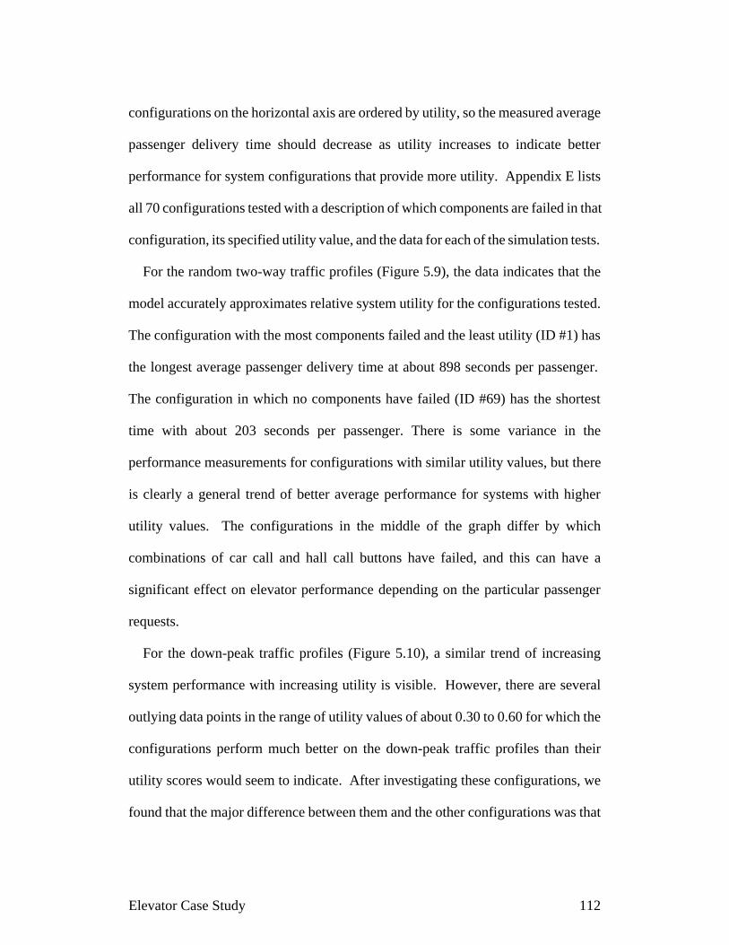
con fig u ra tions on the hor i zon tal axis are or dered by util ity, so the mea sured average

passenger delivery time should decrease as utility increases to indicate better

performance for system configurations that provide more utility. Appendix E lists

all 70 configurations tested with a description of which components are failed in that

configuration, its specified utility value, and the data for each of the simulation tests.

For the random two-way traffic profiles (Figure 5.9), the data indicates that the

model accurately approximates relative system utility for the configurations tested.

The configuration with the most components failed and the least utility (ID #1) has

the longest average passenger delivery time at about 898 seconds per passenger.

The configuration in which no components have failed (ID #69) has the shortest

time with about 203 seconds per passenger. There is some variance in the

performance measurements for configurations with similar utility values, but there

is clearly a general trend of better average performance for systems with higher

utility values. The configurations in the middle of the graph differ by which

combinations of car call and hall call buttons have failed, and this can have a

significant effect on elevator performance depending on the particular passenger

requests.

For the down-peak traffic profiles (Figure 5.10), a similar trend of increasing

system performance with increasing utility is visible. However, there are several

outlying data points in the range of utility values of about 0.30 to 0.60 for which the

configurations perform much better on the down-peak traffic profiles than their

utility scores would seem to indicate. After investigating these configurations, we

found that the major difference between them and the other configurations was that


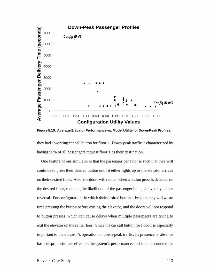
they had a working car call button for floor 1. Down-peak traffic is characterized by

having 90% of all passengers request floor 1 as their destination.

One feature of our simulator is that the passenger behavior is such that they will

continue to press their desired button until it either lights up or the elevator arrives

on their desired floor. Also, the doors will reopen when a button press is detected on

the desired floor, reducing the likelihood of the passenger being delayed by a door

reversal. For configurations in which their desired button is broken, they will waste

time pressing the button before exiting the elevator, and the doors will not respond

to button presses, which can cause delays when multiple passengers are trying to

exit the elevator on the same floor. Since the car call button for floor 1 is especially

important to the elevator’s operation on down-peak traffic, its presence or absence

has a disproportionate effect on the system’s performance, and is not accounted for


0

1000

2000

3000

4000

5000

6000

7000

0.00 0.10 0.20 0.30 0.40 0.50 0.60 0.70 0.80 0.90 1.00


Config ID #1

Config ID #69

Down-Peak Passenger Profiles

Figure 5.10. Average Elevator Performance vs. Model Utility for Down-Peak Profiles.

in our utility model. Thus, configurations in which the car call button is working

will perform much better than their utility values indicate.

For the up-peak traffic profiles (Figure 5.11), the model does not seem to be as

accurate at predicting relative system performance. Many configurations that

supposedly have higher utility values and more working components perform much

worse than configurations with low utility values. This is also due to an unforseen

interaction between the characteristics of the up-peak traffic profiles and the

graceful degradation mechanisms implemented in the system. Since up-peak traffic

is characterized by 90% of the passengers arriving on the first floor to use the

elevator, the drive controller’s default algorithm for visiting floors is actually better

suited for this traffic than the dispatcher’s high performance algorithm.


00.00 0.10 0.20 0.30 0.40 0.50 0.60 0.70 0.80 0.90 1.00


Config ID #1

Config ID #69

Up-Peak Passenger Profiles

1000

2000

3000

4000

5000

6000

7000

Figure 5.11. Average Elevator Performance vs. Model Utility for Up-Peak Profiles.

The default drive controller starts at floor 1, stops at every floor until it reaches

the top floor, and then returns to the first floor to repeat the process unless it receives

an override destination from the dispatcher. For up-peak traffic, this will be very

efficient since most passengers arrive on the first floor and exit on other floors. The

dispatcher’s algorithm will only perform reasonably well for up-peak traffic if the

first-floor hall call button is working. If the first-floor hall call button is broken, the

dispatcher will visit floor 1 periodically, but it will not process the first floor as

frequently as it should for maximum performance, given that 90% of the passengers

arrive there. All of the extreme outlying points in Figure 5.11 were traced to

configurations in which the dispatcher was working but the first-floor hall call

button was not.

Our utility specification gave equal weights to the utility contributions from all

hall call buttons and most car call buttons. We did give the car call button for floor 1

more relative utility value than the other car call buttons, but this did not take into

account its interaction with the door controller. Our experiments indicate that the

utility model was relatively accurate for the general case of random two-way

elevator traffic patterns, but was less accurate for the down-peak and up-peak traffic

profiles. This was partially due to the fact that efficiently processing the up-peak

and down-peak passenger profiles heavily depends on processing the first-floor

button requests. When the first-floor hall call and car call buttons fail, the system’s

performance is severely degraded, and our utility model does not account for this.

These tests indicate that additional hardware redundancy should be added to these

first-floor buttons since they are critical to system performance for the up-peak and

down-peak passenger profiles.


We reran the up-peak and down-peak passenger profile simulations with

modified test configurations in which all the components in the original

configurations were failed except for the first-floor car call and hall call buttons.

These configurations represent situations in which the first-floor buttons have

redundant hardware backups that mask a single button failure. Figures 5.12 and

5.13 show the results of these experiments. Once the first-floor buttons are removed

from the possible failure configurations, our model more closely matches the

performance of the elevator on the up-peak and down-peak passenger profiles.

Additionally the performance of nearly all of the configurations significantly

improves, as all of the average passenger delivery times for all configurations are

less than 1,200 seconds, compared to the previous experiments in which some


Config ID #1Config ID #69


00.00 0.10 0.20 0.30 0.40 0.50 0.60 0.70 0.80 0.90 1.00

Down-Peak with HW Redundant 1st Floor Buttons

Dispatcher Component failed;These configurations use a default

simple dispatching algorithm

1000

2000

3000

4000

5000

6000

7000

Figure 5.12. Average Elevator Performance vs. Model Utility for Down-Peak Profileswith HW Redundant First-Floor Buttons.

configurations had average passenger delivery times as bad as 5,000 or 6,000

seconds.

The dispatcher was designed to optimize performance for the random two-way

passenger profiles, so the model does not completely match the observed

performance for the up-peak and down-peak profiles, even with the first-floor

buttons always working. One way to overcome this might be to specify utility

functions that directly address these specific traffic patterns by giving more weight

to the utility contributions from subsystems that particularly affect the performance

under the special conditions. Then we could use multi-attribute utility theory

[Keeney76, Keeney92] to combine the utility measures from the three traffic profile

types based on which of these traffic types were considered more important to the


Config ID #1 Config ID #69


Up-Peak with HW Redundant 1st Floor Buttons

00.00 0.10 0.20 0.30 0.40 0.50 0.60 0.70 0.80 0.90 1.00

Dispatcher Component failed;These configurations use a default

simple dispatching algorithm

1000

2000

3000

4000

5000

6000

7000

Figure 5.13. Average Elevator Performance vs. Model Utility for Up-Peak Profileswith HW Redundant First-Floor Buttons.

system’s operation. It might also be feasible to design a different dispatching

algorithm for each traffic profile. This would also require that the elevator have

some mechanism for switching modes based on the current traffic pattern.

Another solution might be to build a separate system utility function for each

system mode of behavior that significantly changes utility measures. Each of these

utility functions generates a system utility attribute. For each utility function, a new

set of utility specification parameters would be generated for the system. Then

general system utility would be a linear combination of the different utility

attributes. This effectively multiplies the number specifications required for a

complete utility function, but does not cause an exponential explosion.

5.5 Conclusions

We applied our system model and graceful degradation techniques to an elevator

control system architecture to evaluate how well our model can measure the relative

utility of system configurations, and whether the techniques we propose actually

improve the system’s ability to gracefully degrade. Since in di vid ual com po nent

fail ures sim ply trans form the sys tem from one con fig u ra tion to an other, we can

eval u ate how well the sys tem grace fully de grades by ob serv ing the util ity

dif fer ences among valid sys tem con fig u ra tions. In the el e va tor sys tem, we used our

sys tem model to gen er ate a com plete sys tem util ity func tion for all 8.54 * 1022 valid

sys tem con fig u ra tions by only ex am in ing 424 sub sys tem con fig u ra tions.

The experiments on a simulated implementation of the elevator control system

produced several interesting results. The original elevator design could only


tolerate failures in the car position indicator and car lanterns without failing to

deliver passengers. However, our gracefully degrading elevator design could

withstand up to a loss of 75% of the system’s components and still provide service to

all passengers, albeit at greatly reduced system performance. Ev ery sys tem

con fig u ra tion tested on the gracefully degrading elevator de liv ered all pas sen gers to

their des ti na tions in all sim u la tion tests, sat is fy ing the min i mum el e va tor sys tem

re quire ments de spite a loss of sys tem func tion al ity. We also showed that the utility

model was a good approximation for relative system utility among system

configurations when the elevator traffic was random.

Our utility model did not account for how the elevator’s performance would

depend on particular components for up-peak and down-peak traffic profiles.

Specifically, the first-floor hall call and car call buttons are necessary for the

elevator to provide acceptable utility in these traffic profiles. Since our utility

model assumed that each button subsystem per floor provided an equal contribution

to the overall system utility, this affected our model’s accuracy. This seems to

indicate that even though replicated subsystems may be similarly designed and may

appear homogeneous, system architects should also pay attention to how these

subsystems are used in different system operating modes when evaluating their

utility contribution. In our elevator system model, it would be reasonable to give

more weight to the utility values of the first-floor hall call and car call button feature

subsets relative to the other button feature subsets because they have a large impact

on elevator performance in the up-peak and down-peak modes. In cases where

multiple subsystems are affected by changing system modes, it may be necessary to


specify multiple utility functions based on the different characteristics of these

modes’ operational profiles.

For grace ful deg ra da tion in the el e va tor sys tem we de signed the soft ware

com po nents to have a de fault be hav ior based on their re quired in puts, and to treat

op tional in puts as “ad vice” to im prove func tion al ity when those in puts are

avail able. For ex am ple, the Door Con trol and Drive Con trol com po nents can lis ten

to each other’s com mand out put vari ables in ad di tion to the Drive Speed and Door

Closed sen sors to syn chro nize their be hav ior (open the doors more quickly af ter the

car stops), but only the sen sor val ues are nec es sary for cor rect be hav ior. Like wise,

the Drive Con trol com po nent has a de fault be hav ior that stops the el e va tor at ev ery

floor, but if the De sired Floor sys tem variable is avail able from the out put of the

Dis patcher com po nent, then it can use that value to skip floors that do not have any

pend ing re quests. Also, the Door Con trol com po nent nor mally opens the door for a

spec i fied dwell time, but can re spond to but ton presses to re open the doors if a

pas sen ger ar rives.

We did not ex plic itly design fail ure re cov ery sce nar ios for ev ery pos si ble

com bi na tion of com po nent fail ures in the system, but rather built the in di vid ual

soft ware com po nents to be ro bust to a loss of sys tem in puts. The in di vid ual

com po nents were de signed to ig nore op tional in put vari ables when they were not

avail able and fol low a de fault be hav ior. This is a fun da men tally dif fer ent ap proach

to sys tem-wide grace ful deg ra da tion than spec i fy ing all pos si ble fail ure

com bi na tions to be han dled ahead of time. Prop erties of the soft ware ar chi tec ture

such as the com po nent in ter faces and the iden ti fi ca tion and par ti tion ing of crit i cal

sys tem func tion al ity from the rest of the sys tem seem to be key to achiev ing


sys tem-wide grace ful deg ra da tion. This case study demonstrates the applicability

of our model and techniques to adding graceful degradation to distributed

embedded system designs.


6 Case Study: Autonomous Robot Navigation System

Now that we have demonstrated that we can apply our graceful degradation

techniques to an existing system design, we will use our system model to guide

building a gracefully degrading system from scratch. The CMU Mobot (Mobile

Robot) competition [Mobot2003] provides a rich problem domain in autonomous

vehicle navigation that has several opportunities for graceful degradation

mechanisms. We decided to build a gracefully degrading mobot that could tolerate

multiple sensor and software failures and still complete a race course within our lab.

This chapter details our attempt to build a gracefully degrading mobot system

using our methodology. Section 6.1 describes the mobot navigation problem in

detail. Section 6.2 shows how we used our system model for graceful degradation to

drive our system architecture design and the techniques we used. Section 6.3 details

our implementation and how we built the graceful degradation mechanisms into the

system. Sections 6.4 and 6.5 conclude with the results of our case study.

6.1 Mobot Navigation Problem

The mobot competition involves designing an autonomous robot that can

successfully navigate a race course in the shortest amount of time. The race course

is on an outdoor concrete sidewalk with a white line painted on light gray concrete

pavement. There are several gates placed at different points on the course which the

mobot must pass through in sequential order. At the end of the course the white line

has forks in several directions, and the mobot must pick the path that passes through

the gates in the correct order. Contestants are given the locations of the gates prior

Mobot Case Study 122

to running the race so they can program the mobot ahead of time to follow the

correct path. Each mobot is timed individually and runs the course alone without

interference until it either completes the course or stops making progress.

At first look this seems to be a straightforward line following problem. With the

appropriate sensors and a good line-following algorithm, the only design challenge

would seem to be detecting the points in the course where the line diverges and

taking the correct path. However, there are several features in the environment of

the course that make this problem more interesting. Most mobot designs use some

sort of visual sensor to track the line, such as infrared sensors or an embedded

camera. Since the mobot course is outdoors, the ambient lighting conditions can

vary greatly depending on the weather. Also, the contrast between the white line

and light gray sidewalk pavement is not very large, and the cracks between blocks in

the sidewalk disrupt the continuity of the line. These conditions make line

following more difficult, and the mobots are susceptible to frequently losing track of

the line in the course.

In order to explore graceful degradation opportunities, we generalized the line

following problem to a navigation problem. The line can be treated as a high quality

accurate source of position information that a general navigation system uses to

complete the course. Other sources of location information could include tracking

the cracks in the pavement as the mobot passes over them, and using shaft encoders

on the wheels to measure distance traveled. A navigation algorithm that can take

advantage of the course layout and keep track of its position could anticipate curves

in the line and make more accurate turns to finish the course more quickly.

Additionally, the navigation algorithm should be able to tolerate line sensor failures


and continue to complete the course. If parts of the navigation system fail, the

default line following algorithm can still take over and attempt to complete the

course.

We constructed a smaller mobot course in our lab to run graceful degradation

tests. The lab course uses semi-white masking tape for the line, which contrasts

with the multicolored carpet. Although we do not have to deal with ambient light

changes in the lab, distinguishing the carpet from the line is still a challenge because

the carpet is composed of speckles of colors from near- white to black.

6.2 System Architecture Design

Our goal was to explore software design techniques for graceful degradation.

Rather than completely design the robot hardware, we selected a hardware platform

that provided some of the basic sensors and actuators, could easily accommodate

additional sensor devices, and used a processor that had accessible software

programming support. The basic hardware we started with was an ARobot mobile

robot kit [Arrick2003] with a Basic Stamp 2 processor [Parallax2003]. The robot

consisted of a chassis with three wheels. The front wheel axle has a drive motor for

movement with a shaft encoder for position measurement. The rear wheels are

connected to a servo motor that provides rear wheel steering. The front of the

chassis has two whisker sensors for front collision detection. An embedded

coprocessor on the robot controls the drive motor, servo motor, and encoder, and

communicates via serial I/O to the Basic Stamp processor on the robot. The whisker

sensors are directly connected to the Basic Stamp’s I/O channels. The Basic Stamp


can be programmed to send commands to the coprocessor to control the motors and

read encoder values, and read the values of the whisker sensors. The additional I/O

channels on the Basic Stamp can be used to connect additional sensing devices to

the robot.

With this basic hardware platform, we focused on building a navigation system

that could gracefully degrade when sensors and parts of the navigation system fail.

We took a top down approach and started by specifying the actuators, system

variables and software subsystems that are required for the navigation system.

Figure 6.1 shows the feature subset diagram for the main navigation system.

The Navigation feature subset provides logical movement commands to the

Actuator Control feature subset, which is responsible for moving the mobot to

complete the course. Within the Navigation feature subset, the navigator software

component receives data from the Line Follower, Direction, and Collision

Detection feature subsets, which are derived from sensor subsystems built on the

mobot that are described in the next section. These sensor subsystems can provide

enough data to the navigator to reliably follow the line in the course, and also avoid

obstacles that are sensed by the collision sensors. This is the basic functionality of a

typical mobot system. Having the Direction feature subset so that the mobot knows

what direction it is facing can prevent the mobot from making excessive turns that

could throw it off course. Without any other navigation functionality, if the mobot

ever lost track of the line, it would not be able to complete the course.

In order to compensate for a possible failure of the Line Follower feature subset,

the Navigator also receives data from the Path Planner feature subset. This feature

subset contains a Path Planner software component that receives data from Location


feature subsets and a Map Data component to synthesize the mobot’s current

position, and determine the best route for completing the course. The Map Data

component provides a list of waypoint coordinates that will take the mobot on a path

through the course. The Path Planner will then send a suggested location change

command relative to the mobot’s current position, that the Navigator can interpret

into actual movement commands for the drive and servo motors. This navigation is

based on using all available sensors to monitor the mobot’s current location on the




Actuator


Strong Dependence

SpeedCommandDrive MotorController

Servo MotorController

CommandResolver

TurnCommand

Drive MotorSteering Servo Motor

NavigationFeature Subset

NavigationFeature Subset

Navigator

CollisionDetection

Feature Subset

MapData

Server

Line FollowerFeature Subset

X LocationFeature Subset

PathPlanner

Y LocationFeature Subset

XLocationData

YLocationDataMapData

DesiredLocationChange

CollisionSensorData

RelativeLine

Position

NextDestinationCommand

Actuator ControlFeature Subset

DirectionFeatureSubset

DesiredLocationChange

DirectionData



Figure 6.1. Navigation and Actuator Control Feature Subsets.

course, and doing a simple waypoint navigation based on knowledge of the course

geography.

This is an example of using heterogeneous redundancy (Section 4.3.3) to provide

graceful degradation for a critical subsystem (Section 4.3.2). The Navigation

feature subset can continue to provide utility with either simple line following

functionality, or high-performance location navigation.

The location data is split into separate subsystems for the X (axis parallel to

course’s direction) and Y (axis perpendicular to the course’s direction). The X and

Y Location feature subsets use heterogeneous redundancy to provide graceful

degradation of the location data when sensors fail. Several sensor subsystems

contribute to the location feature subsets and provide utility to the rest of the system.

6.2.1 Sensor Subsystems

We designed several sensors based on the hardware already available in the ARobot

kit, and we also mounted some new sensors on the chassis. One of the major sets of

sensors we added was the line following sensor subsystem. This subsystem consists

of an array of infrared (IR) phototransistors and infrared light emitting diodes

(LED) mounted close to the ground on the front of the mobot’s chassis. Each sensor

is a pair of one phototransistor and one LED. The LED shines IR light on the

ground, which is reflected back up to strike the phototransistor. More light will be

reflected from the white line than the rest of the carpet, so the change in the state of

the phototransistor can detect whether or not the sensor is passing over the line. Six

sensors are mounted an inch apart on the front of the mobot, to form an array that is


normally perpendicular to the line when the mobot is travelling on the course. If the

mobot starts to deviate from the line, it can be detected by the change in the IR

sensor values.

Using these IR sensors, we can to a certain extent detect the relative position of

the center of the mobot to the line. When the mobot is to the left of the line, the right

sensors will sense the line, and when the mobot is to the right of the line, the left

sensors will sense the line. As long at least one IR sensor is over the line, we can

estimate the mobot’s relative position, and the Navigator component can use the

Line Follower’s output to calculate a turn that brings the mobot’s center closer to the

line. Figure 6.2 shows the Line Follower and IR Sensors feature subsets, along with

additional sensor subsystems we added.

In addition to using the IR sensors to follow the line, we can also use them to

detect when the mobot has reached a decision point on the course. These decision

points are characterized by a fork in the line that will continue the path in two

directions. The IR sensors can detect this when both left and right sensors that are

on opposite sides of the mobot sense that they are on the line. Once this is detected,

we can choose which path to take. The Decision Point software component can

maintain a list of decision points in the course and keep a history of how many

decision points have already been passed to make the correct choice. Alternately, if

course map data and location information are available from the Map Data

component and X Location feature subsets, this will also provide reliable

information about the correct fork to take on the path.

In Figure 6.2 we also have the feature subset definitions for Collision Detection

and Crack Detection. The Collision Detector simply receives data from the whisker


sensors on the front of the mobot. These whiskers are metal wires that stick out in

front of the mobot’s frame. When the mobot strikes an object, these wires are

pushed backwards and touch terminals on the mobot that complete a circuit. The

middle of the course is free of obstacles, so when the mobot has a collision, this

indicates that mobot is moving off course, and must backtrack. This can also be

used as a rough position measurement, as it is confirmation that the mobot is at the

edge of the course.




Actuator


Strong Dependence

Line FollowerFeature Subset Relative

Line Position

IRSensorData

IR Sensor 0

LineDetector

0

LineData

LineData

LineData

LineData

LineData

LineData

Line DetectorsFeature Subset

Line Follower

Line DetectorsFeature Subset

Decision PointDetector

Map DataServer

X LocationFeature Subset

Pavement CrackSensor

Left WhiskerSensor

Right WhiskerSensor

Crack Data

Collision Data

Collision DetectionFeature Subset

Crack DetectionFeature Subset

CrackDetector

CollisionDetector

LineData

Line Detector 5Feature Subset



IRSensorData

IR Sensor 1

LineDetector

1LineData



2 3 4

Figure 6.2. Line Follower, IR Sensors, Crack Detection, and Collision DetectionFeature Subsets.

The Pavement Crack Sensor is a metal wire that drags along the ground on the

back of the mobot. When the mobot passes over a crack, the wire dips lower,

causing a hook on the other end of the wire to touch a terminal on the mobot. Since

the sidewalk cracks are spaced at regular intervals on the course, this can be used as

another source of position data.

A shaft encoder is already included on the front wheel’s axle for distance

measurements. We also added low resolution wheel revolution sensors on the rear

wheels. These sensors consist of IR sensors mounted on the back of the mobot, with

strips of white tape placed at regular intervals on the rear wheels’ black tires. We

can sense wheel revolutions by counting the number of times the white strips on the

wheels pass under the IR sensors. These sensors are used for position tracking and

dead reckoning, which is described in the next section.

6.2.2 Dead Reckoning and Location Subsystems

The dead reckoning subsystem uses the position tracking wheel sensors to estimate

the mobot’s change in position. Figure 6.3 shows the details of this feature subset.

To calculate the mobot’s speed and direction, we can use the outputs of the

Command Resolver software component that sends the speed and direction

commands to the actuators. Of course, this assumes that the actuators can precisely

execute commands from the Navigation subsystem without any error or inaccuracy.

Therefore, we can also use the wheel position sensors to estimate the mobot’s

change of speed and direction, and compare it with the Command Resolver’s

outputs. The mobot’s speed and direction estimates are combined with the wheel


position data to estimate the mobot’s location, which is output by the Dead

Reckoning Feature Subset as the XLocationData and YLocationData system

variables.

The Dead Reckoning Feature Subset provides location data to be incorporated

into the X and Y Location feature subsets. These feature subsets collect position

estimates from the multiple sensor subsystems and synthesize the location data used

by the Navigation feature subset. Figure 6.4 displays the X and Y Location feature

subsets.




Actuator


Strong Dependence

CommandResolver

XLocationData

SpeedData

Front WheelEncoder

Feature Subset Rear WheelRevolutions

Feature Subset

Front WheelShaft Encoder

Right WheelIR Sensor

EncoderCountLeftRevCount

Rear Wheel RevolutionsFeature Subset

Front Wheel EncoderFeature Subset

EncoderCounter

Left WheelIR Sensor

Left WheelRev Counter

Right WheelRev Counter

RightRevCount

Front WheelEncoder

Feature SubsetRear WheelRevolutions

Feature Subset

SpeedEstimator

Rear WheelRevolutions

Feature Subset

CommandResolver

DirectionEstimator

DirectionData

DirectionFeatureSubset

SpeedFeatureSubset

SpeedFeature Subset

YLocationData



DeadReckoner

Front WheelEncoder

Feature Subset

Figure 6.3. Dead Reckoning and Related Feature Subsets.

The software components that make up these feature subsets should be separately

designed based on how X and Y position can be estimated from each sensor’s data.

For example, the line sensors can provide data about the mobot’s Y position based

on the line’s location and the mobot’s position relative to the line. However, the line

sensors are of little use in calculating the mobot’s X position, except possibly at

points in the course where the line turns. The X and Y Location Resolvers must deal

with the possible loss of outputs from these sensor subsystems, and may provide a

less accurate location estimate as a result.

The X and Y location estimates are coupled because they both rely on knowing

the mobot’s current direction to estimate change in position. The mobot’s sensors

periodically record the incremental distance traveled by the mobot, but knowing this

distance without knowing the mobot’s direction relative to the course cannot


XLocationData

Crack DetectionFeature Subset

Collision DetectionFeature Subset


Line FollowerFeature Subset

Map DataServer

X LocationResolver

Crack/CollisionSensor

X EstimatorLine XEstimator

XLocationData

Y Location Feature Subset(Longitudinal Perpendicular to Course)

YLocationData


Y LocationResolver

Crack/CollisionY Estimator

Feature Subset

Line YEstimator

Feature Subset

YLocationData

X Location Feature Subset(Parallel to Course)

YLocationDataYLocation

DataXLocation

Data

XLocationData



Actuator


Strong Dependence


Line XEstimatorFeatureSubset

Crack/CollisionX Estimator

Feature Subset

Map DataServer


XLocationData

Line X EstimatorFeature Subset

Crack/CollisionX Estimator

Feature Subset

XLocationData

Figure 6.4. X and Y Location Feature Subsets.

provide an accurate measurement of position change. Thus, the Direction feature

subset provides inputs to all of the location estimators.

6.2.3 System Interface Design

We used our system model framework to guide how we partitioned the mobot’s

navigation system into subsystems. We used our system model’s feature subset

construct to define logical subsystems of components (as shown in this section),

which led to the definition of logical system interfaces. The components and

interfaces we defined are a result of our goal of making the system gracefully

degradable. The multiple IR line sensors provide functional redundancy (Section

4.3.2) since multiple sensors in the array can fail while the remaining sensors can

still provide line following utility. The X and Y Location feature subsets use the

heterogeneous redundancy (Section 4.3.3) of multiple sensors to synthesize

location information, and can continue providing utility until all of the sensor

subsystems fail. The Navigation subsystem also uses two different algorithms (line

following and position tracking) that require different sets of sensors to provide

heterogeneous redundancy.

Our component and interface definitions are presented in Table 6.1. The system

variable interfaces should, by design, facilitate graceful degradation. We broke the

system into several logical subsystems based on sensor and actuator functionality,

and identified pieces of the system that could serve as redundant resources. As

specified in the feature subsets, we should design many of the components to treat

inputs as optional whenever possible. There are 42 components in the system,



Component Component Type System Variable Inputs System Variable Outputs

Steering Servo Motor Actuator Raw Servo Control Data Environment

Drive Motor Actuator Raw Motor Control Data Environment

IR Sensors 0..5 Sensor Environment IRSensorData 0..5

Pavement Crack Sensor Sensor Environment Raw Whisker Data

Left/Right Whisker Sensors Sensor Environment Raw Whisker Data

Front Wheel Shaft Encoder Sensor Environment Raw Encoder beats

Left/Right Rear Wheel IRSensors Sensor Environment IRSensorData L/R

Servo Motor Controller Software TurnCommand Raw Servo Control Data

Drive Motor Controller Software SpeedCommand (Spd Cmd) Raw Motor Control Data

Command Resolver Software NextDestinationCommand TurnCommand, Spd Cmd

Navigator Software

RelativeLinePositon,DirectionData,DesiredLocationChange,CollisionSensorData

NextDestinationCommand

PathPlanner Software MapData, XLocationData,YLocationData DesiredLocationChange

Map Data Server Software N/A MapData

Line Detector 0..5 Software IRSensorData 0..6 LineData 0..5

Line Follower Software LineData 0..6,DecisionPointData RelativeLinePosition

Decision Point Detector Software LineData 0..6, MapData,XLocationData DecisionPointData

Crack Detector Software Raw Whisker Data CrackData

Collision Detector Software Raw Whisker Data CollisionData

Encoder Counter Software Raw Encoder beats EncoderCount

Left/Right WheelRevolution Counters Software IRSensorData L/R Left/RightRevCount

Speed Estimator Software SpeedCommand,EncoderCount, L/RRevCount SpeedData

Direction Estimator Software TurnCommand, EncoderCount,L/RRevCount DirectionData

Dead Reckoner Software SpeedData, DirectionData,EncoderCount, L/RRevCount X/YLocationData

X/Y Line Estimator Software RelativeLinePosition,DirectionData, MapData X/YLocationData

X/Y Crack/CollsionEstimator Software CrackData, CollsionData,

DirectionData, MapData X/YLocationData

X/Y Location Resolver Software X/Y Location Data X/YLocationData

Table 6.1. Mobot Navigation System Component and Interface Specification.

meaning there are 242 (more than 4 * 1012) possible system component

configurations. We have used our system model to organize these components into

24 feature subsets. The number of feature subset configurations for which utility

functions must be specified to generate the system utility function from our model is

156. Since only one feature subset provides outputs to actuators and encapsulates

all of the other feature subsets, it is not necessary to specify system capability

configurations. The system has one functional capability that drives the mobot to

move in the course, specified by the Actuator Control feature subset. Appendix F

details our utility model for the mobot system. The next section describes our

implementation of this software system and how the components are allocated to the

mobot’s hardware.

6.3 Implementation

The mobot has very limited resources in terms of programming space. The Basic

Stamp 2 has only 2 KB for both code and data, and the ARobot’s coprocessor is

already preprogrammed to control the shaft encoder, servo and drive motors, and

cannot be readily reprogrammed. The coprocessor provides an interface through a

serial I/O channel to the Basic Stamp to allow us to send serial commands that will

make the coprocessor operate the motors or read encoder data. Therefore, the Basic

Stamp processor must use its I/O to handle most of the sensors in the system. This

leaves little room for navigation algorithms. We decided to use a general purpose

laptop PC to host all of the system’s navigation algorithms. The PC communicates

with the Basic Stamp processor on the mobot via serial I/O interface. We


programmed the Basic Stamp to periodically sample the sensors and send this data

to the PC, which would then send navigation commands based on the mobot’s

current state. The mobot is tethered to the PC with a serial cable, allowing it free

movement while periodically communicating with the PC.

We implemented the software components defined in our system model as

subroutines running on the Basic Stamp written in the its PBASIC programming

language and as objects in Java running on the PC that communicate via the serial

interface. Figure 6.5 shows the hardware allocation of the software components in

our mobot system. Most of the navigation components are allocated to the PC,

while the software to control the sensors and actuators are allocated to the ARobot’s

processors. The limitations of the hardware available prevented us from using a

more evenly distributed hardware system, but we can still observe how well the


CrackDetector

CollisionDetector

Servo MotorController

Drive MotorController

CommandResolver

Drive MotorSteeringServo Motor

EncoderCounter

Drive WheelShaft Encoder

CrackSensor

Left/RightWhiskerSensors

Left/RightRear WheelIR Sensors

IR SensorArray

Line Detectors0-5

Left/RightWheel RevCounters

Serial I/ONetwork

Connection

ARobot EmbeddedCoprocessor

ARobotBasic Stamp 2Microcontroller

Serial I/ONetwork

Connection

Map DataServer Path PlannerNavigator

Line Follower

Decision PointDetector

Y LocationResolver


Y EstimatorLine Y

Estimator

X LocationResolver


X Estimator

Line XEstimator

SpeedEstimator

DirectionEstimator

DeadReckoner

Laptop PC


Actuator

Hardware Component

Figure 6.5. Hardware Allocation of the Mobot Navigation System.

system gracefully degrades by injecting failures for individual software components

and sensors.

6.4 Experimental Results

We ran several tests of the mobot in our lab to evaluate how well the mobot

performed graceful degradation. The configurations we tested included ones in

which the line follower software component and line sensors were broken, as well as

ones in which the location and dead reckoning components were broken. Since our

tests were run in the lab, and the course we used did not have decision points or

sidewalk cracks, we did not implement the Decision Point Detector or the Crack

X/Y Location Estimator components for these tests. The course in our lab was about

seven feet long by four feet wide. For each configuration, we measured the distance

the mobot went off track at the end of the course, as well as the time the mobot took

to complete the course. We ran 10 tests for each configuration.

Table 6.2 describes these configurations, as well as their utility values predicted

by the model. The performance metric for each configuration is calculated by the

formula:

System Performance = 5/D + 1/T

where D is the average distance the mobot was off course and T is the average time

the mobot took to complete the course in that configuration across the 10

measurements. These particular parameters are arbitrary, but we used this formula

to give heavier weight to the mobot’s ability to stay on the track compared to how

fast it finished the course. Figure 6.6 graphically displays the results of our tests.


Graph 6.6-A plots the utility value of each configuration versus the measured

performance metric. Graph 6.6-B shows the time it took for each configuration to

complete the course. Graphs 6.6-C and 6.6-D show how far the mobot was off

course, both in terms of distance and percentage of the width of the course. For each

configuration in graphs 6.6-B,C and D, the line represents the range of the values

measured for the ten experiments run, and the middle bar represents the arithmetic

mean of the tests.

As shown in the graphs and table, the configurations with dead reckoning, and

combined dead reckoning and line following perform better than the other

configurations, matching our utility model’s predictions. They are very close to the

line at the end of the course, and reach their goal quickly. The configuration that

only uses line following makes wide turns at the curves in the course, making it

more difficult to closely follow the line and lengthening the time it takes to finish.


Config ID Components Failed

System Utility Predicted by

the model

SystemPerformance

Metric

1 None (except Decision Point Detector and Crack LocationEstimators) 0.97 2.21

2 Line Sensors, Line Follower Component 0.72 1.69

3 Line Sensors, Line Follower Component, Front WheelEncoder Sensor 0.67 0.17

4 Dead Reckoner Component, X/Y Location ResolverComponent, Path Planner Component 0.49 0.52

5Dead Reckoner Component, X/Y Location ResolverComponent, Path Planner Component, Front Wheel Encoder Sensor

0.46 0.32

6Dead Reckoner Component, X/Y Location ResolverComponent, Path Planner Component, Front Wheel Encoder Sensor, Direction Estimator Component

0.41 0.23

Table 6.2. Mobot Configurations Tested.

One interesting data point is Configuration 3, which has failed line sensors and a

failed front wheel encoder sensor. In this configuration, the mobot must perform

dead reckoning navigation, but with only the rear wheel sensors for both position

and direction information. The rear wheels act as low resolution encoders that

provide less accurate position data, and skew the dead reckoner’s calculations. The

result is that the Navigator computes that it has reached the waypoint at the end of

the course much more quickly because the position data is incorrect. Thus, the

mobot is actually much more off course than the other configurations, but its time

measurement appears to outperform the other configurations. This is why we


C. Mobot Accuracy Results (Raw)

01020

304050

60

1 2 3 4 5 6Mobot Configuration

B. Mobot Time Results

0

10

20

30

40

50


0.00

0.50

1.00

1.50

2.00

2.50

0 0.2 0.4 0.6 0.8 1

0%

20%

40%

60%

80%

100%

120%


D. Mobot Accuracy Results

A. Mobot Utility Vs. Performance

Utility Value

Config 1

Config 6Config 5

Config 4

Config 3

Config 2

Figure 6.6. Mobot Configuration Experiment Results.

account for both accuracy and speed in evaluating the mobot’s performance, with

accuracy being the relatively more important attribute.

The experiments indicate that rear wheel revolution sensors are not accurate

enough to serve as reliable data sources without any other source of position data.

They produce erroneous outputs, which breaks our fail-fast, fail-silent assumption.

Thus the configuration that only has these sensors available has a much lower

performance score compared to its utility value predicted by the model. This

analysis indicates that these sensors should be improved to provide more accurate

data or removed from the system so that they do not cause a system failure.

We did try running the mobot outdoors on the CMU Mobot course, but the results

were not as successful. The mobot was able to follow the line for a short distance,

but the turning radius of the robot made it difficult to track the line accurately.

Figure 6.7 displays a section of the official mobot course. The limitations of the

mobot’s hardware made it difficult to implement more complex control algorithms

beyond simple bang-bang and proportional control.


4 ft

4 ft

White Line

Figure 6.7. Middle Portion of the Official Mobot Course (Adapted from an Image at[Mobot2003]).

6.5 Summary

In this chapter we have demonstrated the use of our methodology to build a

gracefully degrading autonomous robot system. We started with a basic hardware

platform, added some sensor systems, and constructed a navigation system based on

the sensors available. We used our system model to guide the definition of

hierarchical feature subsets that use heterogeneous redundancy to provide graceful

degradation. This graceful degradation allowed the mobot to successfully navigate

the course when subsystems fail. The component and interface definitions were

designed to provide graceful degradation by breaking the system into logical

partitions that could be decoupled from one another. We focused on designing the

system to tolerate multiple sensor failures since we were limited in the hardware to

one set of system actuators. Starting with feature subset definitions enabled us to

logically define the software components and interfaces to produce a gracefully

degrading navigation system.

This case study illustrates how embedded software system design can be severely

constrained by the hardware resources. Ideally, we would prefer allocating the

software components across more hardware nodes, but we were limited by the

system’s hardware platform. Despite this limitation, we were able to build the

mobot’s software system such that it could tolerate multiple IR sensor failures.

Additionally, the mobot can tolerate a loss of the location navigation subsystem and

continue to complete the course with simple line following.


7 Conclusions

This dissertation has presented a methodology for scalable specification, analysis,

and design of graceful degradation in distributed embedded systems. An ideal

gracefully degrading system minimizes the cumulative loss of system utility as

successive system component failures occur. We designed a modeling framework

that reduces the exponential effort required to specify the relative utility of all 2N

system configurations of N components. We then applied this modeling framework

to some example embedded system architectures to identify some heuristic design

techniques that can enhance a system’s ability to gracefully degrade. We

demonstrated the scalability of our system model and the applicability of our design

techniques on two representative distributed embedded system architectures.

Section 7.1 revisits the proposed contributions of this thesis from Chapter 1, and

summarizes how they have been fulfilled. Section 7.2 deals with the basic

assumptions we made for building our system model and design techniques. We

also explore the relevant system issues that affect the applicability of our

methodology. Section 7.3 provides a discussion of future work and possible

extensions of this research. Section 7.4 ends with a discussion of the results of this

research.

Conclusions 142

7.1 Summary of Contributions

This thesis proposed a system model, analysis technique, and design techniques for

scalable graceful degradation in distributed embedded systems. In the Introduction

(Chapter 1) we proposed four major contributions of this research:

• A structural model derived from the system’s software architecture

specification that enables scalable specification of grace ful deg ra da tion in

embedded systems, and expresses many current hardware and software

fault tolerance techniques in a single framework.

• A proposed set of design principles that will promote system-wide grace ful

deg ra da tion in distributed embedded systems that were identified as a result

of applying the system model.

• An analysis technique that uses the model to provide hints to where to

focus design effort for improving graceful degradation and can validate that

the implementation achieves graceful degradation.

• Two case studies in which we applied our system model and design

techniques to representative distributed embedded system applications and

observed how well they could gracefully degrade.

Each of these contributions is discussed below.

7.1.1 System Model for Specifying Graceful Degradation

Our system model allows scalable specification of graceful degradation by

exploiting the hierarchical partitioning of the system architecture that groups

system components into subsystems. Our graceful degradation model uses utility as

Conclusions 143

a general measure of the system’s ability to satisfy its functional and dependability

requirements. We can generate a system utility function that specifies the relative

utility of all 2N possible system configurations of N components at the cost of

O(N*2k) utility evaluations, where k is the maximum number of components in an

individual subsystem. This utility function allows us to evaluate how well the

system gracefully degrades, because we can directly see how component failures

(which alter the system configuration) affect system utility.

Our view of real-time embedded software systems consists of software

components that represent periodic tasks that receive sensor data or state

information, process this data and provide outputs to the rest of the system. The

sensors are the data sources for the system, and the actuators are the data sinks that

provide functionality based on the data values sent by their software controllers. At

the architectural level, the traditional component and connector view captures

relevant data dependencies among the software components. In hardware, these

tasks are distributed across several processor nodes connected by a real-time

broadcast network. The tasks communicate by periodically sending network

messages that contain their output data.

In our model’s software view, the components are represented as software

components, sensors, and actuators, and the connectors are represented as system

variables that represent data values passed among the components. We then

partition the data flow graph of the software system into feature subset graphs that

represent logical subsystems. These feature subsets are in general not disjoint and

can share logical components across subsystems. This is necessary to capture the

logical software dependencies in the system architecture without making

Conclusions 144

assumptions about how components are allocated in hardware. For example, a

single sensor could provide data to multiple subsystems by transmitting it on the

network, or each subsystem could have its own redundant sensor. We also annotate

the system variable connections between components based on dependency. A

component can depend strongly or weakly on a system variable input, or treat that

input as an optional “enhancing” input. We use these dependency relationships to

identify all of the valid component configurations of all feature subsets, and then use

their hierarchical organization to compose the overall system utility function.

The hardware view of our model is orthogonal to the software view and provides

the allocation information about which components are running on which processor

nodes. This view also identifies which components are replicated in hardware for

reliability, and enables traditional reliability analysis techniques that account for

hardware failures. A set of identical replicated components represents one software

component in the software view. We can examine the effect of hardware failures on

system utility by removing all of the components that were running on a failed node

(provided there are no replicas running on other nodes) from the software

configuration, and recalculating the utility.

7.1.2 Design Techniques for Graceful Degradation

We applied our system model to a hypothetical distributed embedded system

architecture that was designed to provide graceful degradation to identify

Conclusions 145

organizational properties that should enhance graceful degradation. The properties

we identified include:

Specifying well-defined interfaces that decouple software components in the

system. The interfaces among components determine the system variables in our

model and thus how feature subsets are partitioned. The architecture should have a

set of interfaces that represent intermediate computational steps that allow logical

decoupling of subsystems. Our techniques for graceful degradation concentrate on

making components robust to input failures, and providing redundant sources of

system variables to tolerate subsystem failures. If the architecture does not have

interfaces that promote hierarchical decoupling of its subsystems, these techniques

may become cost prohibitive. If a system has few defined system variables, this

would imply that feature subsets are large, monolithic, and complex, making them

more difficult to design so that they can tolerate input errors and satisfy the fail-fast

fail-silent fault assumption. If a system has many feature subsets that require many

different system variables, it will be difficult to provide enough redundant resources

to output these system variables and tolerate subsystem failures.

Adding limited redundant resources to critical subsystems that are necessary

for system functionality. One of the benefits of our system model is that we can use

the dependency relationships among components to immediately identify which

components and feature subsets are required for the system to provide any utility at

all. We can concentrate fault tolerance design effort and redundant resources on

preserving these parts of the system, rather than replicating every component in the

system for dependability. As long as the system obeys our initial fault assumptions,

Conclusions 146

then components that are identified as non-critical cannot adversely affect the

operation of critical components and subsystems.

Exploiting heterogeneous system resources to provide auxiliary redundancy

through common system interfaces. Many embedded systems are designed to

optimize resources to provide a large set of features and functionality. Many of the

system resources that provide these features can be viewed as functionally

equivalent and actually provide a redundant backup when a component failure

occurs. For example, multiple sensors that provide different levels of accuracy for a

measurement, or measure different aspects of the same environmental phenomena

can provide redundant data sources when combined with a software component that

transforms the sensor data to a common system variable interface. This technique

exploits redundancy inherent in the system architecture and does not require

additional system resources to tolerate a failure.

De sign ing com po nents with de fault be hav iors that take over when in puts from

other com po nents are lost. As a complementary approach to providing redundant

sources of system variable inputs, we also propose designing components to treat

their inputs as optional whenever possible to reduce their dependency on inputs.

Our initial approach to accomplishing this is to identify the minimum service a

component must provide and the minimum inputs it requires for this service. Then

we design a behavior that can satisfy this minimum functionality requirement in

addition to the component’s normal behavior. The component will provide its full

functionality when all of its inputs are available, but if an input failure is detected,

the component will switch to its simple backup behavior until the input is restored.

If there are multiple inputs that can potentially fail, the component can be designed

Conclusions 147

with multiple algorithms depending on the amount of design effort that can be

spared to make this component robust to input failures.

7.1.3 Analysis for Validating Graceful Degradation

We can use our system model to analyze the system architecture to target which

components and feature subsets should receive graceful degradation support. We

use the scalable system utility function generated from the system model and

evaluate system configurations to identify which components and feature subsets

contribute significantly to overall system utility. We then target these parts of the

system for graceful degradation improvements using the design techniques we have

already identified. Any components or feature subsets that are single points of

failure or drastically reduce system utility when not available should be targeted for

graceful degradation mechanisms.

The model analysis provides information about which feature subsets and

components are critical to system utility, allowing us to target these parts of the

system for graceful degradation mechanisms. Choosing which techniques to

implement requires an analysis of the tradeoffs between the resources available in

the system and the level of dependability required. Our scalable specification

framework should enable these tradeoffs to be explicitly identified with the utility

model and information about the resources required for system components and

feature subsets.

In addition to using the model at design time to determine where graceful

degradation mechanisms should be applied in the system, the model can also be

Conclusions 148

used to validate whether or not the system implementation achieves the level of

graceful degradation predicted. In general the utility model should reflect each

component and feature subset’s contribution to system utility. If we have a utility

metric that incorporates some or all of the desired system properties defined in the

system’s requirements, and these attributes can be measured in the system

implementation, then the relative differences between the utility of system

configurations predicted by the model should match the actual measured utility

differences of these configurations in the implementation. If there are

configurations that do not fit the expected rankings, they may indicate either an

inaccuracy in the system model, a dependability problem in the system

implementation, or a violation of the model’s assumptions in the system design. We

can use this analysis iteratively to both refine the system model and identify

dependability bottlenecks in the system implementation.

7.1.4 Case Studies that Illustrate the Methodology

We presented two case studies in which we applied our system model, analysis, and

design techniques to develop a gracefully degrading embedded system architecture.

The first was an existing, detailed elevator system architecture that was

implemented in a discrete event simulation. The elevator architecture and

implementation had already been thoroughly exercised through several iterations

on a distributed embedded systems class design project. When we applied our

model and graceful degradation techniques to this elevator system, the

Conclusions 149

implementation was able to tolerate many more component failures than the original

elevator design.

The major improvements we made to the system included adding software

components that could synthesize floor sensor messages from the car speed and

position sensors (adding heterogeneous redundancy to critical subsystems), thus

providing a backup for failed floor sensors; modifying the dispatcher software

component to periodically synthesize floor requests for floors that had failed

buttons (designing components to be robust to input failures); and modifying the

drive controller to follow a default pattern of periodically visiting all floors when the

dispatcher input is lost (designing components to be robust to input failures). These

changes required very little extra code in the implementation (a 9% increase in total

lines of code of the control system) and made the system resistant to up to 75% total

system component failures.

We also ran experiments to measure how well our system utility model predicted

the relative utility values of different elevator configurations, in terms of

minimizing average passenger travel time. We ran tests on the three major types of

elevator traffic: normal two-way traffic, up-peak traffic, and down-peak traffic. Our

model was relatively accurate for the two-way traffic cases, but was significantly

less accurate with the up-peak and down-peak traffic profiles. This was due to the

fact that up-peak and down-peak traffic are heavily dependent on the operation of

the first-floor buttons to provide efficient service, and our utility model did not

account for that. Our conclusion is that replicated subsystems that are similarly

designed do not always have an equal effect on system utility. Special cases such as

the first-floor hall call and car call buttons should be given different weights in the

Conclusions 150

utility model to account for their impact on system utility. In cases where the system

has multiple operating modes that affect the utility contributions of many

subsystems, it might be necessary to develop multiple utility parameters for utility

models in the system based on the system’s operational profiles, and design a

multi-attribute utility function that gives more weight to the utility values based on

more likely or more important scenarios.

The second case study involved the design of a gracefully degrading autonomous

mobot (mobile robot). The mobot must navigate a race course without getting lost

by following a white line. We started with an off the shelf robot kit with three

wheels, a motor, encoder, servo, whisker collision sensors, and two embedded

processors, and added several sensor systems such as infrared line sensors, a

pavement crack detector, and rear wheel revolution sensors to provide opportunities

for graceful degradation. We used our system model to build a software system that

can gracefully degrade when combinations of sensors fail. We were successful in

that the robot could separately tolerate both a failure of the line sensors, as well as a

failure of the navigation subsystem and still complete a test course we designed in

the lab. This case study also demonstrated that hardware constraints and limitations

can have an affect on the implementation of the “ideal” software system as

envisioned in our system model.

7.2 Assumptions and System Design Issues

The applicability of our system model and graceful degradation techniques is

predicated on several assumptions about the system being designed. We have

Conclusions 151

narrowed our focus to distributed embedded real-time systems and specified a fault

model. There are also some design issues that are not addressed in this thesis that

will affect how this methodology can be applied to embedded system architectures,

such as the feasibility of designing all software components to be robust to input

failures, and exactly how designers construct their system and feature subset utility

evaluations.

7.2.1 Embedded System Architecture and Fault Model

Our system model was specifically designed to be applicable to distributed

embedded system architectures. We focus on the software architecture of the

application, and make some assumptions about the system’s hardware and network

organization. We assume the network uses broadcast communication among nodes

so that the software architecture is decoupled from the system communication

mechanisms. We also assume that there are sufficient hardware resources available

to satisfy memory, bandwidth, and real-time requirements. Our graceful

degradation techniques emphasize how to modify the components that make up the

software system to tolerate component failures.

Our model as sumes a fail-fast, fail-si lent fault model with per fect fault de tec tion.

How ever, we can re lax this as sump tion based on how we con strain the sys tem

ar chi tec ture and the dis trib uted na ture of the sys tem. For grace ful deg ra da tion we

are more con cerned with the ef fects a fault pro duces rather than the source of the

fault. In or der to min i mize the fail ures a fault can pro duce, as well as min i mize fault

prop a ga tion, we con strain our sys tem ar chi tec ture to only al low com mu ni ca tion

Conclusions 152

among soft ware com po nents via sys tem vari ables. As long as the im ple men ta tion

ad heres to the ar chi tec ture and does not pro vide hid den com mu ni ca tion chan nels

among soft ware com po nents, faults can only be prop a gated through the de fined

sys tem vari ables.

We be lieve the fail-fast, fail-si lent fault model is a rea son able as sump tion

be cause we are only con cerned with faults that cause cor rup tion of the sys tem

vari ables’ state, and this cor rup tion can be readily de tected by the sys tem vari ables’

re ceiv ers. We do not en vi sion a cen tral ized fail ure de tec tion in fra struc ture, which

it self could be a sin gle point of fail ure, but rather soft ware com po nents that val i date

their sys tem vari able in puts as they are up dated and only use those in puts if they

pass the val i da tion tests. Sim ple checks on the in put vari ables can catch many

er rors, and scale with the num ber of in puts per soft ware com po nent. This fault

model can cover several types of the component failures described below.

A soft ware com po nent could fail to up date a sys tem vari able at the ap pro pri ate

time; a sys tem vari able could be cor rupted to an in valid state ei ther by the sender,

re ceiver, or com mu ni ca tion me dium; or the sys tem vari able could be cor rupted to a

valid but in cor rect state. In a real-time sys tem, fail ure to up date a sys tem vari able

can be de tected as its dead lines are missed. If a sys tem vari able be comes stale, i.e. it

has n’t been up dated for sev eral pe ri ods, then the re ceiv ers of that vari able can

as sume that the sender has failed or is un reach able. If re ceiv ers de tect in valid data

in a sys tem vari able for mul ti ple con sec u tive pe ri ods, then they can as sume that the

sender has failed. The most dif fi cult fail ure to de tect is when a sys tem vari able has

valid but in cor rect data. These fail ures can not be eas ily dis tin guished from a cor rect

Conclusions 153

sys tem vari able that is man i fested by an ex cep tional con di tion oc cur ring in the

en vi ron ment.

7.2.2 Generating the System Utility Model

Specifying the utility model is still a challenging problem. A comprehensive

quantitative utility model that accounts for all relevant functionality and

dependability properties is a significant undertaking. We have built a framework

that reduces the number and scope of utility analyses to be within individual

subsystems. A system designer can qualitatively rank the component

configurations of individual feature subsets, so that we can approximate utility

functions by generating linear functions for each configuration based on the

component utilities. We assume that the system is decoupled so that the form of the

utility function of each feature subset is only dependent on the component

configuration rather than each component’s utility value.

We must also relate feature subset utility to overall system utility. We use the

functional capability definitions to accomplish this, and they are based on the fact

that most architectures are decomposed into major subsystems that each provide

functionality. At the system level, these functional capabilities each contain feature

subsets that can contribute to their utility. The system utility function is then based

on the configuration of functional capabilities, and the utility functions defined for

each configuration. The system utility function is heavily dependent on the

definition of the functional capabilities, which must be specified according to which

feature subsets provide which functionality.

Conclusions 154

There is a possibility that our system model may achieve scalable utility analysis

at the expense of accounting for how interactions between components and

subsystems affect system utility. If components and subsystems are tightly coupled,

it may be necessary to build a more complex utility model using multi-attribute

utility theory [Keeney76, Keeney92] that explicitly accounts for couplings between

system components. Designers may also want to develop a more detailed utility

model that explicitly identifies utility attributes, to analyze trade-offs among

competing system properties such as performance and dependability. An

architectural analysis method such as the Architecture Trade-off and Analysis

Method (ATAM) [Kazman98] that evaluates system quality attributes may aid

development of a multi-attribute utility model.

7.3 Future Work

This thesis is a first step towards a general methodology for graceful degradation.

There are several challenges for this research that could be extensions of this work.

Some future extensions include building a tool to automatically generate the system

model and utility function from a system’s architectural specification, relaxing

some of the assumptions of our model and extending the model to be applicable to

other types of computer systems and software architectures, identifying other

graceful degradation design techniques, and using our view of system

configurations to build product family architectures.

Generating the system model from software component and interface

specifications is relatively straightforward, so building a semi-automated tool

Conclusions 155

should be a reasonable extension. The software data flow graph can be generated by

connecting the input and output interfaces of software components, and the feature

subsets can be defined by creating subgraphs at each interface boundary. Valid

feature subset configurations can be identified by traversing input and output

dependency links between components and determining which components are

required for each feature subset to provide minimum utility.

We have had some success with building a prototype tool that can parse a text

specification that lists all system variables, components, and each component’s

input and output interface. This is sufficient to generate a system model with feature

subset definitions. The process is not completely automated, as a designer still must

verify that the feature subsets capture the subsystems he or she designed into the

system, specify the system’s functional capabilities in terms of which feature

subsets provide which system functionality, and generate the utility function

parameters for each feature subset configuration. It should be possible to build a

tool that can extract relevant information for our model from software architecture

specifications that are expressed in an architecture description language (ADL)

such as Acme [Garlan2000] that emphasizes component and connector definitions.

Currently our model makes several assumptions that narrow its applicability to

distributed embedded systems, and our design techniques for scalable graceful

degradation are predicated on these assumptions. Our model assumes that the

individual software components are strongly decoupled, and can only affect each

other though the defined communication interfaces. However, many software

systems may have hidden dependencies between components in their

implementation that can allow faults to propagate. For example, components that

Conclusions 156

run in the same process may have access to the same memory space, so that a defect

in one component may cause it to overwrite another component’s data and

subsequently cause errors in other parts of the system. Our system model may still

be applicable in these situations if a more sophisticated fault model that accounts for

more pernicious failures due to software defects can be mapped to how component

failures affect the system’s configuration.

Since we have made sys tem vari ables a key mech a nism in our sys tem

ar chi tec ture, it may be desirable to specify how these vari ables rep re sent their

ac cu racy or qual ity as a part of their sys tem state. This would aid utility evaluation

because a component and feature subset’s utility value could be mapped to the

quality of its output variables. One ap proach would be to rep re sent data ac cu racy as

a range of un cer tainty or con fi dence in ter val. This might work well for nu mer i cal

data types and is flex i ble in that the ac cu racy of a sys tem vari able can be

dy nam i cally up dated while the sys tem is run ning. How ever, this ap proach might

re quire a heavy weight an a lyt i cal model for each pro ducer of the sys tem vari able

that would be costly to im ple ment. Ad di tionally, this model would not work well

for non-nu meric and categorical sys tem vari able data types.

An other ap proach would be to spec ify the qual ity of data for the out puts of each

soft ware com po nent at de sign time. The sys tem de sign ers could rank soft ware

com po nents that pro duce the same sys tem vari ables based on the al go rithms they

use. This static rank ing would then be used at run time by the re ceiv ers of the

sys tem vari ables to de ter mine which ones to use. Ad di tionally, sim i lar data from

dif fer ent send ers that have sig nif i cant qual i ta tive dif fer ences could be de fined as

two sep a rate sys tem vari ables. This ap proach has the ad van tage of re quir ing fewer

Conclusions 157

sys tem re sources to im ple ment and is rea son able when there are not many

in de pend ent sources of the same sys tem vari able. The draw backs of this ap proach

are that it is less flex i ble since changes in sys tem vari able qual ity dur ing runtime

can not be de tected, and re ceiv ers of sys tem vari ables have a heavier bur den in

de cid ing which in puts to use.

Our view of the system is that components only communicate via data flow in

system variables, but there are many other architectural patterns in which control

flow rather than data flow is the major connection between components. To

generate feature subset definitions and valid component configurations, we focus on

the dependency relationships among the components, which manifest as data flow

relationships in distributed embedded systems. It may be that we can still use our

model to represent dependency relationships, but they may represent different

connector mechanisms for different architectural patterns.

The graceful degradation design techniques we have proposed do not represent

all possible mechanisms, but rather what we identified using our model. The fact

that we are able to represent many current software fault tolerance techniques gives

us some confidence that this model can be used to identify other graceful

degradation opportunities. We have specifically focused on techniques that are

integrated into the software architecture to provide immediate failover mechanisms

when faults are detected, and do not depend on global fault detection and

reconfiguration to recover from errors. We view reconfiguration as a

complementary approach that can provide more recovery alternatives beyond our

failover approach, such as reallocating software components to different processor

Conclusions 158

nodes and restarting failed components. There may also be other techniques that

can be developed from work in research in self-healing systems [WOSS2002].

Our model was initially designed to enable scalable specification of utility

differences between different software component failure configurations in a

system, but it can also be used as a view of a product family architecture. Each

product instance could be represented by a different component configuration. A

high-end product would have a configuration with most of the components present

and providing functionality, while a low-end product’s configuration may only have

enough components to provide minimum functionality. The parallel between a

gracefully degrading system and a product family architecture could be exploited to

provide systems that naturally gracefully degrade by design.

7.4 Concluding Thoughts

Graceful degradation mechanisms can offer improved system dependability with

few redundant resources, but at the cost of additional system design effort. Prior to

this work, comprehensive system-wide graceful degradation required an

exponential specification and design effort with respect to the system component

faults being covered. This thesis provides a methodology for evaluating and

designing scalable graceful degradation for distributed embedded systems by taking

advantage of the hierarchical structure of these system’s architectures.

Graceful degradation is especially important for distributed embedded systems

because these systems typically cannot afford the additional system resources

required for fault tolerance mechanisms that maintain both system dependability

Conclusions 159

and complete functionality. Graceful degradation is an alternative to brute force

redundancy that can potentially provide the same level of dependability at the

expense of reduced functionality when failures occur. This research indicates that

distributed embedded systems can exploit graceful degradation opportunities

because a significant portion of these systems is designed to provide enhanced or

auxiliary functionality above the functionality required to satisfy the system’s

primary mission.

Hierarchical decomposition is the best technique designers have for managing

functional complexity, and our model for specifying graceful degradation exploits

this to achieve scalability. Building a gracefully degrading system can increase the

system’s complexity, and our system model provides a mechanism for managing

this complexity without sacrificing graceful degradation opportunities. We restrict

our design techniques to the component and subsystem level to limit the total impact

of these techniques on system complexity. As systems become more complex with

added features and functionality, techniques for scalable graceful degradation will

become increasingly important for managing system failure modes. Our model for

evaluating the utility of system configurations enables scalable analysis and design

of graceful degradation in distributed embedded system architectures.

Conclusions 160

8 References

[Abdelzaher97] Abdelzaher, T.F., Atkins, E.M., Shin, K.G., “QoS Negotiation inReal-Time Systems and its Application to Automated Flight Control,”Proceedings of the Third IEEE Real-Time Technology andApplications Symposium, Montreal, Quebec, Canada, June 1997, pp.228-238.

[Adlemo95] Adlemo, A., Andreasson, S.-A., “Improved Availability inManufacturing Systems Through Graceful Degradation: Case Study ofa Machining Cell,” Proceedings of the 1995 IEEE InternationalConference on Robotics and Automation, Nagoya, Japan, May 1995,pp. 1744-1750.

[Arrick2003] ARobot Robot Kit for Experimenters and Educators, Arrick Robotics,<http://www.robotics.com/arobot>, 2003.

[Arora98] Arora, A., Kulkarni, S.S., “Component Based Design ofMultitolerance,” IEEE Transactions on Software Engineering, Vol. 24, No.1, January 1998, pp. 63-78.

[Avizienis85] Avizienis, A., “The N-version approach to fault-tolerant software,”IEEE Transactions on Software Engineering, SE-11(12), December1985, pp. 1491-1501.

[Avizienis2001] Avizienis, A., Laprie, J.-C., and Randell, B., Fundamental Concepts of Dependability, Research Report N01145, LAAS-CNRS, April 2001.

[Banks94] Banks, S., Coleman, N., et al., “Architecture Based Approach toControl Software Design,” Proceedings of the 1994 American ControlConference, Baltimore, MD, USA, June 1994, pp. 2731-2735.

[Bass98] Bass, L., Clements, P., Kazman, R., Software Architecture in Practice,Addison-Wesley, Reading, Massachusetts, 1998.

[Boasson98] Boasson, M., “Software Architecture for Distributed ReactiveSystems,” Twenty-Fifth Conference on Current Trends in Theory andPractice in Informatics (SOFSEM ‘98), Jasna, Slovakia, November1998, pp. 1-18.

[Bodson93] Bodson , M., Lehoczky, J., et al., “Control reconfiguration in thepresence of software failures,” Proceedings of the 32nd IEEEConference on Decision and Control, San Antonio, TX, USA,December 1993, pp. 2284-2289.

[Botti2000] Botti, O., De Florio, V., et al., “The TIRAN Approach to ReusingSoftware Implemented Fault Tolerance,” Proceedings 8th EuromicroWorkshop on Parallel and Distributed Processing, Rhodos, Greece,January 2000, pp. 325-332.

References 161

[Dvorak2000] Dvorak, R., Rasmussen, G., et al., “Software Architecture Themes inJPL’s Mission Data System,” Proceedings of 2000 IEEE AerospaceConference, Vol. 7, Big Sky, MT, USA, March 2000, pp. 258-269.

[Garlan2000] Garlan, D., Monroe, R.T., Wile, D., “Acme: Architectural Descriptionof Component-Based Systems,” Foundations of Component-BasedSystems, G.T. Leavens and M. Sitaraman (eds), Cambridge UniversityPress, 2000, pp. 47-68.

[Herlihy 91] Herlihy, M. P., Wing, J. M., “Specifying Graceful Degradation,” IEEE Transactions on Parallel and Distributed Systems, Vol.2, No.1, 1991,pp. 93-104.

[Jayanti99] Jayanti, P., Chandra, T.D., Toueg, S., “The Cost of GracefulDegradation for Omission Failures,” Information Processing Letters,Vol. 71, No. 3-4, 1999, pp.167-172.

[Jurgen99] Jurgen, R.K., ed., Automotive Electronics Handbook, Second Edition,McGraw-Hill, New York, 1999.

[Kazman97] Kazman, R., Clements, P., et al., “Classifying Architectural Elementsas a Foundation for Mechanism Matching,” Proceedings Twenty-FirstAnnual International Computer Software and Applications Conference (COMPSAC’97), Washington, DC, USA, August 13-15, 1997, pp.14-17.

[Kazman98] R. Kazman, M. Klein, M. Barbacci, H. Lipson, T. Longstaff, andS.J.Carrière, “The ArchitectureTradeoff Analysis Method,”Proceedings of 4th International Conference on Engineering ofComplex Computer Systems (ICECCS’98), Monterey, CA, August1998, pp. 68-78.

[Keeney76] Keeney, R.L., Raiffa, H., Decisions with Multiple Objectives:Preference and Value Tradeoffs, John Wiley & Sons, New York, 1976.

[Keeney92] Keeney, R.L., Value-Focused Thinking: A Path to CreativeDecisionmaking, Harvard University Press, Cambridge, MA, 1992.

[Knight85] Knight, J.C., Leveson, N.G., St. Jean, J.D., “A Large Scale Experiment in N-version Programming,” Fifteenth Annual InternationalSymposium on Fault-Tolerant Computing, Ann Arbor, MI, USA, June1985, pp. 135-139.

[Knight2000] Knight, J.C., Sullivan, K.J., “On the Definition of Survivability,”University of Virginia, Department of Computer Science, TechnicalReport CS-TR-33-00, 2000.

[Knight2003] Knight, J.C., Strunk, E.A., Sullivan, K.J., “Towards a RigorousDefinition of Information System Survivability,” DISCEX 2003,Washington DC, April 2003.

References 162

[Koopman99] Koopman, P., DeVale, J., “Comparing the Robustness of POSIXOperating Systems,” Twenty-Ninth Annual International Symposiumon Fault-Tolerant Computing, Madison, WI, USA, June 1999, pp.30-37.

[Kopetz97] Kopetz, H., Real-Time Systems: Design Principles for DistributedEmbedded Applications, Kluwer Academic Publishers, Boston, 1997.

[Lamport82] Lamport, L., Shostak, R., and Pease, M., “The Byzantine GeneralsProblem”, ACM Transactions on Programming Languages andSystems 4, No. 3, July 1982, pp. 382-401.

[Laprie87] Laprie, J., Arlat, J., et al., “Hardware- and Software-Fault Tolerance:Definition and Analysis of Architectural Solutions,” SeventeenthInternational Symposium on Fault-Tolerant Computing, Pittsburgh,PA, July 1987, pp. 116-121.

[Latronico2001] Latronico, B., Martin, C. and Koopman, P., “Analyzing Dependabilityof Embedded Systems from the User Perspective,” Workshop onReliability in Embedded Systems (in conjunction with Symposium onReliable Distributed Systems/SRDS-2001), New Orleans, LA, October2001.

[Losq77] Losq, J., “Effects of Failures on Gracefully Degradable Systems,” 7thAnnual International Conference on Fault-Tolerant Computing, LosAngeles, CA, USA, June 1977, pp. 29-34.

[Lyu95] Lyu, M., ed., Software Fault Tolerance, John Wiley & Sons,Chichester, 1995.

[Medvidovic97] Medvidovic, N., Taylor, R.N., “A Framework for Classifying andComparing Architectural Description Languages,” SoftwareEngineering Notes 22, No. 6, November 1997, pp. 60-76.

[Meyer78] Meyer, J.F., “On Evaluating the Performability of DegradableComputing Systems,” The Eighth Annual International Conference onFault-Tolerant Computing (FTCS-8), Toulouse, France, June 1978, pp. 44-49.

[Meyer93] Meyer, J.F., Sanders, W.H., “Specification and Construction ofPerformability Models,” Proceedings of the Second InternationalWorkshop on Performability Modeling of Computer andCommunication Systems, Mont Saint-Michel, France, June 1993.

[Mittal98] Mittal, A., Manimaran, G., Murthy, C.S.R., “Integrated DynamicScheduling of Hard and QoS Degradable Real-Time Tasks inMultiprocessor Systems,” Proceedings of the Fifth InternationalConference on Real-Time Computing Systems and Applications,Hiroshima, Japan, October 1998, pp. 127-136.

[Mobot2003] Carnegie Mellon School of Computer Science 9th Annual MobotRaces, <http://www-2.cs.cmu.edu/~mobot>, 2003.

References 163

[Nace2000] Nace, W., Koopman, P., “A Product Family Approach to GracefulDegradation,” International Workshop on Distributed and ParallelEmbedded Systems (DIPES), October 2000, pp. 131-140.

[Nace2002] Nace, W., “Graceful Degradation via System-wide Customization forDis trib uted Em bedded Sys tems,” Ph.D. dis ser ta tion, Dept. of Electrical And Computer Engineering, Carnegie Mellon University, May 2002.

[Ng77] Ng, Y.-W., Avizienis, A., “A Reliability Model for GracefullyDegrading and Repairable Fault-Tolerant Systems,” 7th AnnualInternational Conference on Fault-Tolerant Computing, Los Angeles,CA, USA, June 1977, pp. 22-28.

[Patton93] Patton, R. J., Chen, J., “Advances in Fault Diagnosis Using AnalyticalRedundancy,” IEE Colloquium on Plant Optimisation for Profit(Integrated Operations Management and Control), London, UK,January 1993, pp. 6/1 - 6/12.

[Parallax2003] Basic Stamp 2 Microcontroller, Parallax, Inc.,<http://www.parallax.com>, 2003.

[Randell75] Randell, B., “System Structure for Software Fault Tolerance,” IEEETransactions on Software Engineering, vol. SE-1, No. 2, June 1975,pp. 220-232.

[Ramanathan97] Ramanathan, P., “Graceful Degradation in Real-Time ControlApplications Using (m, k)-firm Guarantee,” 27th Annual internationalConferences on Fault-Tolerant Computing, Seattle, WA, USA, June1997, pp. 132-141.

[Rasmussen2001] Rasmussen, R., “Goal-Based Fault Tolerance for Space Systems usingthe Mission Data System,” 2001 IEEE Aerospace Conference, Vol. 5,March 2001, Big Sky, MT, pp. 2401-2405.

[Ravindran97] Ravindran, B., Welch, L.R., Kelling, C., “Building DistributedScalable Dependable Real-Time Systems,” Proceedings InternationalConference and Workshop on Engineering of Computer-BasedSystems, Monterey, CA, USA, March 1997, pp. 452-459.

[Rennels84] Rennels, D., “Fault-Tolerant Computing - Concepts and Examples”,IEEE Transactions on Computers C-33, No. 12, December 1984, pp.1116-1129.

[Rostamzadeh95] Rostamzadeh, B., Lonn, H., et al., “DACAPO: A DistributedComputer Architecture for Safety-Critical Control Applications,”Proceedings of the Intelligent Vehicles ’95 Symposium, Detroit, MI,USA, September 1995, pp. 376-381.

[Rushby99] Rushby, J., “Partitioning in Avionics Architectures: Requirements,Mechanisms, and Assurance,” NASA Contractor ReportCR-1999-209347, June 1999.

References 164

[Rushby2001] Rushby, John, “A Comparison of Bus Architectures for Safety-CriticalEmbedded Systems,” Computer Science Laboratory, SRI InternationalTechnical Report, September, 2001.

[Shaw96] Shaw, M., Garlan, D., Software Architecture: Perspectives on anEmerging Discipline, Prentice Hall, Upper Saddle River, New Jersey,1996.

[Shaw97] Shaw, M., Clements, P., “A Field Guide to Boxology: PreliminaryClassification of Architectural Styles for Software Systems,”Proceedings of the 21st International Computer Software andApplications Conference (COMPSAC ‘97), August 1997, pp. 6-13.

[Strakosch98] Strakosch, G.R., ed., The Vertical Transportation Handbook, ThirdEdition, John Wiley & Sons, Inc., New York, 1998.

[Verissimo2001] Verissimo, P., Rodrigues, L., Distributed Systems for SystemArchitects, Kluwer Academic Publishers, Boston, 2001.

[Wang99] Wang, W.-L., Wu, Y., Chen, M.-H., “An Architecture-Based Software Reliability Model,” Proceedings 1999 Pacific Rim InternationalSymposium on Dependable Computing, Hong Kong, December 1999,pp. 143-150.

[Weber89] Weber, D.G., “Formal Specification of Fault-Tolerance and itsRelation to Computer Security,” Proceedings of Fifth InternationalWorkshop on Software Specification and Design, Pittsburgh, PA, USA, May 1989, pp. 273-277.

[WOSS2002] First Workshop on Self-Healing Systems (WOSS 2002), ACM Press,Charleston, South Carolina, November 2002.

Thesis Publications:

[Shelton2001] Shelton, C., Koopman, P., “De veloping a Soft ware Ar chi tec ture forGrace ful Deg ra da tion in an El e va tor Con trol Sys tem,” Work shop onRe li abil ity in Em bedded Sys tems (in con junc tion with Sym po sium onRe li able Dis trib uted Sys tems/SRDS-2001), New Or leans, LA, Oc to ber2001.

[Shelton2002] Shelton, C., Koopman, P., “Using Architectural Properties to Modeland Measure System-Wide Graceful Degradation,” Workshop onArchitecting Dependable Systems sponsored by the InternationalConference on Software Engineering (ICSE2002), Orlando, FL, May2002.

[Shelton 2003] Shelton, C., Koopman, P., Nace, W., “A Framework for ScalableAnalysis and Design of System-wide Grace ful Deg ra da tion inDis trib uted Em bedded Sys tems,” To appear in the Eighth IEEEInternational Workshop on Ob ject-ori ented Real-time De pend ableSys tems (WORDS 2003), Guadalajara, Mexico, January 2003.

References 165

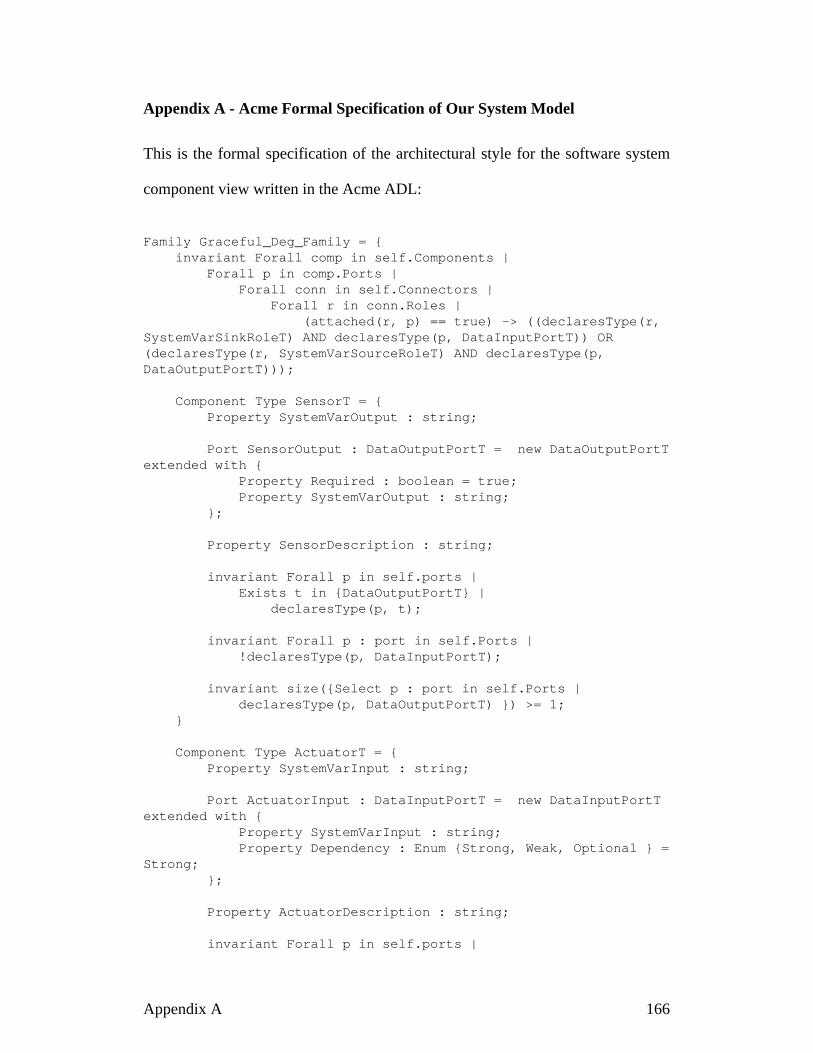
Appendix A - Acme Formal Specification of Our System Model

This is the formal specification of the architectural style for the software system

component view written in the Acme ADL:

Family Graceful_Deg_Family = { invariant Forall comp in self.Components | Forall p in comp.Ports | Forall conn in self.Connectors | Forall r in conn.Roles | (attached(r, p) == true) -> ((declaresType(r,SystemVarSinkRoleT) AND declaresType(p, DataInputPortT)) OR(declaresType(r, SystemVarSourceRoleT) AND declaresType(p,DataOutputPortT)));

Component Type SensorT = { Property SystemVarOutput : string; Port SensorOutput : DataOutputPortT = new DataOutputPortT extended with { Property Required : boolean = true; Property SystemVarOutput : string; }; Property SensorDescription : string; invariant Forall p in self.ports | Exists t in {DataOutputPortT} | declaresType(p, t);

invariant Forall p : port in self.Ports | !declaresType(p, DataInputPortT);

invariant size({Select p : port in self.Ports | declaresType(p, DataOutputPortT) }) >= 1; }

Component Type ActuatorT = { Property SystemVarInput : string; Port ActuatorInput : DataInputPortT = new DataInputPortTextended with { Property SystemVarInput : string; Property Dependency : Enum {Strong, Weak, Optional } = Strong; }; Property ActuatorDescription : string; invariant Forall p in self.ports |

Appendix A 166

Exists t in {DataInputPortT} | declaresType(p, t);

invariant Forall p : port in self.Ports | !declaresType(p, DataOutputPortT); invariant size({Select p : port in self.Ports | declaresType(p, DataInputPortT) }) >= 1; }

Component Type SoftwareComponentT = { Property ComponentDescription : string; invariant size({Select p : port in self.Ports | declaresType(p, DataOutputPortT) }) >= 1; invariant Forall p in self.ports | Exists t in {DataInputPortT, DataOutputPortT} | declaresType(p, t) <vis-ports : boolean = true;>; }

Port Type DataInputPortT = { Property SystemVarInput : string; Property Dependency : Enum {Strong, Weak, Optional }; } Port Type DataOutputPortT = { Property SystemVarOutput : string; Property Required : boolean; } Connector Type SystemVariableConnT = { Property SystemVarData : string; invariant size({Select r : role in self.Roles | declaresType(r, SystemVarSourceRoleT) }) >= 1; invariant size({Select r : role in self.Roles | declaresType(r, SystemVarSinkRoleT) }) >= 1; invariant Forall r in self.roles | Exists t in {SystemVarSinkRoleT, SystemVarSourceRoleT} | declaresType(r, t); }

Role Type SystemVarSourceRoleT = { Property SystemVarData : string; } Role Type SystemVarSinkRoleT = { Property SystemVarData : string; }}

Appendix A 167

Appendix B - Utility Specification for the Automobile Navigation System

This appendix contains all of the feature subset and utility definitions for the

automobile navigation system presented in Chapter 4. The numbers chosen in the

utility specification are an arbitrary representation of how a system designer with

knowledge of the system could assign utility values based on the functionality of

each subsystem. We start with the “low level” feature subsets that contribute to

providing location data in the navigation system. Figure B.1 shows the hierarchical

definitions of these feature subsets, and Table B.1 shows the utility functions

generated for these feature subsets.

Appendix B 168

CurrentDirectionBestDead

Reckoner

GPS NullReckoner

SpeedFeature Subset

CurrentLocation


GroundSpeed

BetterDead

Reckoner

GoodDead

Reckoner

SimpleDead

Reckoner

GPS1

CurrentLocationRaw


ThrottleAngle

CvtWheelSpeed

SpeedFeature Subset GroundSpeed

SpeedIntegrator1 Speed

Integrator2

GPS1

VDC MM1 EngineSensor

AccelerationAvgWheelSpeed

YawRate

YawGenerator


CurrentDirection

DirIntegrator

GPS1

LWS MM1SboxSteering

Angle

Compass



CurrentLocation




GroundSpeed GroundSpeed GroundSpeed




YawRate





Figure B.1. Expansion of the Location Feature Subset.

Figure B.2 shows the feature subsets that comprise the Map and two of the eight

Display feature subsets. Each Display feature subset requires location and map data

to provide functionality. Figure B.3 gives the feature subset diagrams for the other

six Display feature subsets.

Appendix B 169


VDC Speed {VDC Sensor, CvtWheelSpeed} UVDC = 1

All other configurations UVDC = 0

MM1 Speed {MM1 Sensor, Speed Integrator1} UMM1 = 1

All other configurations UMM1 = 0

Engine Speed Est {Engine Speed Sensor, Speed Integrator2} UEngine = 1

All other configurations UEngine = 0

Speed

Any of the 15 combinations of {GPS1 sensor(ugps), VDC Speed Feature, MM1 SpeedFeature, Engine Speed Est Feature} in which atleast one is working

USpeed = Max(1*ugps1,0.75*UVDC, 0.85*UMM1,0.6*UEngine)

All components failed USpeed = 0

Yaw Rate Any configuration in which either the Sboxsensor (usbox) or MM1 sensor (umm1) is working UYaw = Max(1*usbox, 0.8*umm1)

{LWS sensor, Yaw Generator} UYaw = 0.6

All other configurations UYaw = 0

Direction Any configuration in which either the GPS1sensor or Compass sensor (ucompass) is working UDir = Max(1*ugps1, 0.9*ucompass)

{Yaw Rate Feature, DirIntegrator} UDir = 0.2 + 0.6*UYaw

All other configurations UDir = 0

Dead Reckoning

Any configuration with at least one deadreckoning software component (Simple DeadReckoner (usdr), Good Dead Reckoner (ugdr),Better Dead Reckoner (ubtdr), Best DeadReckoner (ubedr)) and both Speed and DirectionFeatures

UDR = Max(0.2*usdr, 0.4*ugdr,0.6*ubtdr, 0.7*ubedr) + 0.2*UDir +0.1*USpeed

All other configurations UDR = 0

Location{GPS1 sensor, GPS Null Reckoner (ugpsnr)} or{GPS1 sensor, GPS Null Reckoner, DeadReckoning Feature}

ULocation = 1

{Dead Reckoning Feature, GPS Null Reckoner}or {Dead Reckoning Feature, GPS1 Sensor} ULocation = 0.8*UDR

All other configurations ULocation = 0

Table B.1. Utility Specification for the Location and Related Feature Subsets.

Appendix B 170

Display


Map04DisplayMap

MapImage




RenderMap

MapImage

MapData



PathInfo

CurrentLocation

Display


Map08DisplayMap




RenderMap2

MapDrawCommands

MapData



PathInfo

CurrentLocation

MapDrawCommands

CurrentLocation

MapDataServer

LocationSentry

Map DVD


MapDataRaw

UpdateMap

MapData



Actuator

Feature Subset BoundaryStrong Dependence

Figure B.2. Partial Expansion of Display Feature Subsets.

Display

Map03DisplayMap

MapImage





PathInfo

CurrentLocation

Display

Map07DisplayMap

MapDrawCommands





PathInfoCurrentLocation

Display

Map06DisplayMap

MapDrawCommands




CurrentLocation

Display

Map05DisplayMap

MapDrawCommands




CurrentLocation

Display

Map01DisplayMap

MapImage




CurrentLocation

Display

Map02DisplayMap

MapImage




CurrentLocation

Figure B.3. Diagrams of the Remaining Display Feature Subsets.

Table B.2 shows the utility specifications for the Display and Map feature

subsets. These feature subsets cannot tolerate component failures, but the feature

Appendix B 171


Map Data {MapDVD Sensor, Location Feature Subset,Location Sentry, MapDataServer} UMapData = 0.7 + 0.3*ULocation

All other configurations UMapData = 0

RenderMap {Map Data Feature Subset, RenderMap} URMap = 0.4 + 0.6*UMapData

All other configurations URMap = 0

RenderMap2 {Map Data Feature Subset, RenderMap2} URMap2 = 0.4 + 0.6*UMapData

All other configurations URMap2 = 0

Display01 {Location Feature Subset, RenderMap FeatureSubset, Display Actuator, Map01}

UD1 = 0.5 + 0.2*ULocation +0.3*URMap

All other configurations UD1 = 0

Display02 {Location Feature Subset, RenderMap FeatureSubset, Display Actuator, Map02}

UD2 = 0.5 + 0.2*ULocation +0.3*URMap


Display 03{Location Feature Subset, RenderMap FeatureSubset, Path Planner Feature Subset, DisplayActuator, Map03}

UD3 = 0.5 + 0.2*ULocation +0.2*URMap + 0.1*UPath


Display04{Location Feature Subset, RenderMap FeatureSubset, Path Planner Feature Subset, DisplayActuator, Map04}

UD4 = 0.5 + 0.2*ULocation +0.2*URMap + 0.1*UPath


Display05 {Location Feature Subset, RenderMap2 FeatureSubset, Display Actuator, Map05}

UD5 = 0.5 + 0.2*ULocation +0.3*URMap2


Display06 {Location Feature Subset, RenderMap2 FeatureSubset, Display Actuator, Map06}

UD6 = 0.5 + 0.2*ULocation +0.3*URMap2


Display07{Location Feature Subset, RenderMap2 FeatureSubset, Path Planner Feature Subset, DisplayActuator, Map07}

UD7 = 0.5 + 0.2*ULocation +0.2*URMap2 + 0.1*UPath


Display08{Location Feature Subset, RenderMap2 FeatureSubset, Path Planner Feature Subset, DisplayActuator, Map08}

UD8 = 0.5 + 0.2*ULocation +0.2*URMap2 + 0.1*UPath


Table B.2. Utility Specification for the Map and Display Feature Subsets.

subsets themselves are redundant backups for each other to provide the Display

actuator’s functionality.

Figure B.4 diagrams the Path Planner, Turn Signal, Speaker, and related feature

subsets, and Table B.3 gives their utility specification in our model. These feature

subsets represent the alternative functionality available in the navigation system in

Appendix B 172


MapDataCurrentLocation


PathInfo


UserInterface

Destination

TurnInfo

Text

TurnSound

TurnInfoCvt2

TurnInfoCvt

SpeechSynth

SpeechSynthSimple

Speaker



TurnSpeakerDriver Speaker

Commands

TurnInfo

Turn SignalIndicator


TurnInfoFeatureSubset

TurnSignalDriver

TurnSignalCommands

CurrentLocationTurnInfo

Gen1


LocationFeature Subset Path Planner

Feature Subset

TurnInfo

PathInfo

TurnInfoGen2

TurnInfoGen3

TurnInfoGen4

TurnSound




Actuator


PathPlanner

Figure B.4. Expansion of Turn Signal and Speaker Feature Subsets.

the event that the Display fails. Navigation information can still be communicated

to the driver through the Speaker and Turn Signal actuators.

With a complete specification for the utility of all feature subset configurations,

we can generate a system utility function using the utility values of the feature

subsets encapsulated in the system functional capabilities. Figure B.5 describes

these capabilities and the feature subsets they contain, and Table B.4 describes their

utility functions along with the system utility function in terms of capability

utilities. For any system configuration, the utility value can be generated by

recursively evaluating the utility values of the functional capabilities and their

feature subsets based on which components are present in the configuration.

Appendix B 173


Path Planner {User Interface Sensor, Map Data FeatureSubset, Location Feature Subset, Path Planner}

UPath = 0.5 + 0.2*UMapData +0.3*ULocation

All other configurations UPath = 0

Turn Info

Any configuration with at least one turn infosoftware component (TurnInfo1 (uti1), TurnInfo2(uti2), TurnInfo3 (uti3), TurnInfo4 (uti4)) and bothLocation and Path Planner Features

UTurnInfo = 0.6 * Max(1*uti1,0.8*uti2, 0.6*uti3, 0.4*uti4) + 0.2 * UPath + 0.2 * ULocation

All other configurations UTurnInfo = 0

Sound CommandAny configuration in which the Turn Info FeatureSubset, TurnInfoCvt, and SpeechSynth areworking

USound = 0.6 * 0.4*UTurnInfo

{Turn Info Feature Subset, TurnInfoCvt2,SpeechSynthSimple} USound = 0.5 * 0.4*UTurnInfo

{Turn Info Feature Subset, SpeechSynthSimple} USound = 0.5 * 0.4*UTurnInfo

{Turn Info Feature Subset, TurnInfoCvt2} USound = 0.3 * 0.4*UTurnInfo

All other configurations USound = 0

Speaker {Sound Command Feature Subset, TurnSpeaker Driver, Speaker Actuator} USpeaker = 0.3 + 0.7*USound

All other configurations USpeaker = 0

Turn Signal {Turn Info Feature Subset, Turn Signal Driver,Turn Signal Indicator Actuator} UTurnSignal = 0.6 + 0.4*UTurnInfo

All other configurations UTurnSignal = 0

Table B.3. Utility Specification for the Path Planner, Speaker, and Turn SignalFeature Subsets.

Appendix B 174

Display Capability Turn Signal Capability




Speaker Capability


Figure B.5. System-Level Functional Capabilities and their Feature Subsets.

System Capability Con fig u ra tion Util ity Func tion

Speaker {Speaker Feature Subset} USpeakerCapability = USpeaker

Speaker Feature Subset failed USpeaker = 0

Turn Signal {Turn Signal Feature Subset} UTurnSignalCapability = UTurnSignal

Turn Signal Feature Subset failed UTurnSignalCapability = 0

DisplayAny of the 63 configurations in which there is atleast of the eight Display Feature Subsets(Display01 - Display08)

UDisplayCapability = Max(1*UD4,0.9*UD8, 0.8*UD3, 0.7*UD7,0.6*UD2, 0.5*UD6, 0.4*UD1,0.3*UD5)

All Display Feature Subsets failed UDisplayCapability = 0

System Utility All Capability ConfigurationsUSystem = 0.6*UDisplayCapability +0.2*USpeakerCapability +0.1*UTurnSignalCapability

Table B.4. Utility Specification for System Functional Capabilities.

Appendix C - Interface Specification for the Elevator System Components

This appendix contains the interface specification of the elevator system software

components, taken from the original elevator requirements document. For clarity,

we first provide the elevator sensor and actuator message descriptions from Chapter

5. In the fol low ing no ta tion, the val ues within the “[ ]” brack ets rep re sent the

stan dard rep li ca tion of an ar ray of sen sors or ac tu a tors, and the val ues within the “(

)” pa ren the ses rep re sent the val ues the sen sor or ac tu a tor can out put. For ex am ple,

the Hall call mes sage type maps to an ar ray of sen sors for the up and down but tons

on each floor out side the el e va tor that is f (the num ber of floors the el e va tor

ser vices) by d (the di rec tion of the but ton; Up or Down) wide, and each but ton

sen sor can ei ther have a value v of True (pressed) or False (not pressed). Un less

oth er wise noted, “f” rep re sents the num ber of floors the el e va tor ser vices, “d”

rep re sents a vari able that in di cates a di rec tion of ei ther Up or Down, “j” is a vari able

that is a value of ei ther Left or Right (for the left and right el e va tor doors), and “v”

de notes a value that can be ei ther True or False.

The sen sor mes sage types avail able in the sys tem in clude:

• AtFloor[f](v): Out put of AtFloor sen sors that sense when the car is near a

floor.

• CarCall[f](v): Out put of car call but ton sen sors lo cated in the car.

• CarLevelPosition(x): Out put of car po si tion sen sor that tracks where the

car is in the hoistway. x = {distance value from bot tom of hoistway in

millimeters}

• CarWeight(w): Output of car weight sensor that measures the aggregate

weight of all passengers in the car. w = { weight in car in pounds }

Appendix C 175

• DoorClosed[j](v): Out put of door closed sen sors that will be True when

the door is fully closed.

• DoorOpen[j](v): Out put of door open sen sors that will be True when the

door is fully open.

• DoorReversal[j](v): Out put of door re ver sal sen sors that will be True

when door senses an ob struc tion in the door way.

• HallCall[f,d](v): Out put of hall call but ton sen sors that are lo cated in

hall way out side the el e va tor on each floor. Note that there are a to tal of 2f -

2 rather than 2f hall call but tons since the top floor only has a down but ton

and the bot tom floor only has an up but ton.

• HoistwayLimit[d](v): Out put of safety limit sen sors in the hoistway that

will be True when the car has over run ei ther the top or bot tom hoistway

lim its.

• DriveSpeed(s,d): Out put of the main drive speed sen sor. s = {speed value},

d = {Up, Down, Stop}

The ac tu a tor com mand messages avail able in the sys tem are:

• DesiredFloor(f, d): Com mand from the el e va tor dis patcher al go rithm

indicating the next floor des ti na tion. d = {Up, Down, Stop} (This is not an

ac tu a tor in put, but rather an in ter nal vari able in the con trol sys tem sent

from the dis patcher to the drive controller)

• DesiredDwell(n): Command from the elevator dispatcher algorithm to the

door controllers indicating how long the doors should remain open when

stopped on a floor. n = { Integer dwell time in milliseconds } (This is also

Appendix C 176

not an actuator input, but an internal control system variable that allows the

dispatcher to affect the operation of the door motors)

• DoorMotor[j](m): Door mo tor com mands for each door. m = {Open,

Close, Stop}

• Drive(s, d): Com mands for 2-speed main el e va tor drive. s = {Fast, Slow,

Stop}, d = {Up, Down, Stop}

• CarLantern[d](v): Com mands to con trol the car lan tern lights; Up/Down

lights on the car doorframe used by pas sen gers to de ter mine the el e va tor’s

cur rent trav el ing di rec tion.

• CarLight[f](v): Com mands to con trol the car call but ton lights in side the

car call but tons to in di cate when a floor has been se lected.

• CarPositionIndicator(f): Com mands for po si tion in di ca tor light in the car

that tells us ers what floor the car is ap proach ing.

• HallLight[f,d](v): Com mands for hall call but ton lights in side the hall call

but tons to in di cate when pas sen gers want the el e va tor on a cer tain floor.

• EmergencyBrake(v): Emer gency stop brake that should be ac ti vated

when ever the sys tem state be comes un safe and the el e va tor must be shut

down to pre vent a cat a strophic failure.

Software Components in the Elevator:

Safety Monitor - Monitors system sensors and controllers to ensure safe

operation and trigger emergency shut down when necessary.

Inputs: AtFloor[1..f], DoorClosed[Left, Right], DoorReversal[Left, Right],

DriveSpeed, HoistwayLimit[Up, Down], Drive, DoorMotor[Left, Right]

Output: EmergencyBrake

Appendix C 177

Drive Controller - Controls drive motor to move elevator in hoistway.

Inputs: AtFloor[1..f], CarLevelPosition, DoorClosed[Left, Right],

DoorMotor[Left, Right], DriveSpeed, Hoistwaylimit[Up, Down], DesiredFloor,

EmergencyBrake

Output: Drive

Door Controller[j] - Controls the door motors to operate the elevator doors. One

door controller class instantiated as two software door controller objects that each

control one door.

Inputs: AtFloor[1..f], DoorClosed[j]. DoorOpen[j], DoorReversal[j],

DesiredFloor, DesiredDwell, DriveSpeed, Drive, CarCall[1..f], HallCall[1..f, (Up,

Down)]

Output: DoorMotor[j]

Car Call Controller[f] - Monitors car call button sensors to provide car button

information to the system and light the car button light. One car button controller

class is instantiated f times for each button.

Inputs:CarCall[f] (from sensor), AtFloor[f], DoorClosed[Left, Right]

Outputs: CarCall[f] (to the network), CarLight[f]

Hall Call Controller[f, d] - Monitors hall call button sensors to provide hall

button information to the system and light the hall button light. One hall button

controller class is instantiated 2f - 2 times for each button.

Inputs: HallCall[f, d] (from sensor), AtFloor[f], DoorClosed[Left, Right],

DesiredFloor

Outputs: HallCall[f, d] (to the network), HallLight[f, d]

Appendix C 178

Dispatcher - Determines elevator’s next destination based on passenger requests

Inputs: CarCall[1..f], HallCall[1..f, (Up, Down)], CarWeight, DoorClosed[Left,

Right], DriveSpeed, AtFloor[1..f]

Outputs: DesiredFloor, DesiredDwell

Lantern Controller[d] - Operate passenger feedback lights that indicate

elevator’s travelling direction when the elevator is stopped on a floor. One

controller class is instantiated as two software lantern controller objects that control

each light.

Inputs: DesiredFloor, AtFloor[1..f], DoorClosed[Left, Right]

Output: CarLantern[d]

Car Position Indicator Controller - Operates passenger feedback lights that

indicate next floor the elevator will reach as it travels in the hoistway.

Inputs: AtFloor[1..f], DesiredFloor, DriveSpeed, CarLevelPosition

Output: CarPositionIndicator

Virtual AtFloor Controller[f] - Software controller that outputs AtFloor

messages when an Atfloor sensor fails. One virtual atfloor controller class is

instantiated f times for each AtFloor sensor.

Inputs: AtFloor[f] (from sensor to detect failure), DriveSpeed, CarLevelPosition

Outputs: AtFloor[f]

Appendix C 179

Appendix D - Utility Specification for the Elevator System

This appendix lists the utility functions we specified for the elevator system in

Chapter 5.

Appendix D 180



Any configuration in which at least one of the two sensors: Hoistway Limit Up Sensor (uhoistwayup),Hoistway Limit Down Sensor (uhoistwaydown) isworking

UHoistway = 0.5*uhoistwayup +0.5*uhoistwaydown

Both Hoistway Limit Sensors Failed UHoistway = 0

Door ClosedSensors

Any configuration in which at least one of the two sensors: Left Door Closed Sensor (uldc), RightDoor Closed Sensor (urdc) is working

UDoorClosed = 0.5*uldc + 0.5*urdc

Both Door Closed Sensors Failed UDoorClosed = 0


Any configuration in which at least one of the two sensors: Left Door Reversal Sensor (uldr), RightDoor Reversal Sensor (urdr) is working

UDoorReversal = 0.5*uldr + 0.5*urdr

Both Door Reversal Sensors Failed UDoorReversal = 0

Safety Monitor

{Safety Monitor Controller, Emergency BrakeActuator, Drive Speed Sensor, Drive ControlFeature Subset, Door Control Feature Subset,Hoistway Limit Sensors Feature Subset, DoorReversal Sensors Feature Subset, Door ClosedSensors Feature Subset, AtFloor SensorsFeature Subset}

USafety = 1

All other configurations USafety = 0

Drive Control

Any configuration with all of these components:{Drive Controller, Drive Motor, Drive SpeedSensor, Safety Monitor Feature Subset,Hoistway Limit Sensors Feature Subset, DoorClosed Sensors Feature Subset, AtFloorSensors Feature Subset} and any combinationof: Car Positon Sensor (ucps), Desired FloorFeature Subset (UDesiredFloor), Door ControlFeature Subset (UDoorControl)

UDrive = 0.1 + 0.2*ucps +0.65*UDesiredFloor +0.05*UDoorControl

All other configurations UDrive = 0

Left/Right DoorControl

Any configuration with all of these components:{Left/Right Door Controller, L/R Door ClosedSensor, L/R Door Open Sensor, L/R DoorReversal Sensor, L/R Door Motor, Drive SpeedSensor, AtFloor Sensors Feature Subset} andany combination of: Drive Control FeatureSubset, DesiredFloor Feature Subset, Car CallButtons Feature Subset (UCarCall), Hall CallButtons Feature Subset (UHallCall)

ULeftDoor = 0.6 + 0.1*UCarCall +0.2*UHallCall + 0.05*UDesiredFloor + 0.05*UDrive

URightDoor = 0.6 + 0.1*UCarCall +0.2*UHallCall + 0.05*UDesiredFloor +0.05*UDrive

All other configurations ULeftDoor = 0; URightDoor = 0

Table D.1. Utility Specification for the Safety, Door and Drive Feature Subsets.

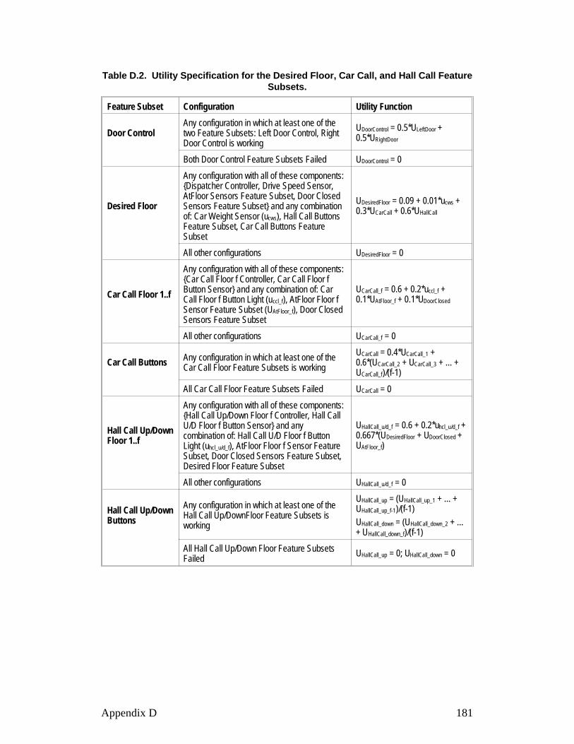
Appendix D 181


Door ControlAny configuration in which at least one of thetwo Feature Subsets: Left Door Control, RightDoor Control is working

UDoorControl = 0.5*ULeftDoor +0.5*URightDoor

Both Door Control Feature Subsets Failed UDoorControl = 0

Desired Floor

Any configuration with all of these components:{Dispatcher Controller, Drive Speed Sensor,AtFloor Sensors Feature Subset, Door ClosedSensors Feature Subset} and any combinationof: Car Weight Sensor (ucws), Hall Call ButtonsFeature Subset, Car Call Buttons FeatureSubset

UDesiredFloor = 0.09 + 0.01*ucws +0.3*UCarCall + 0.6*UHallCall

All other configurations UDesiredFloor = 0

Car Call Floor 1..f

Any configuration with all of these components:{Car Call Floor f Controller, Car Call Floor fButton Sensor} and any combination of: CarCall Floor f Button Light (uccl_f), AtFloor Floor fSensor Feature Subset (UAtFloor_f), Door ClosedSensors Feature Subset

UCarCall_f = 0.6 + 0.2*uccl_f + 0.1*UAtFloor_f + 0.1*UDoorClosed

All other configurations UCarCall_f = 0

Car Call Buttons Any configuration in which at least one of theCar Call Floor Feature Subsets is working

UCarCall = 0.4*UCarCall_1 +0.6*(UCarCall_2 + UCarCall_3 + ... +UCarCall_f)/(f-1)

All Car Call Floor Feature Subsets Failed UCarCall = 0

Hall Call Up/Down Floor 1..f

Any configuration with all of these components:{Hall Call Up/Down Floor f Controller, Hall CallU/D Floor f Button Sensor} and anycombination of: Hall Call U/D Floor f ButtonLight (uhcl_u/d_f), AtFloor Floor f Sensor FeatureSubset, Door Closed Sensors Feature Subset,Desired Floor Feature Subset

UHallCall_u/d_f = 0.6 + 0.2*uhcl_u/d_f + 0.667*(UDesiredFloor + UDoorClosed +UAtFloor_f)

All other configurations UHallCall_u/d_f = 0

Hall Call Up/Down Buttons

Any configuration in which at least one of theHall Call Up/DownFloor Feature Subsets isworking

UHallCall_up = (UHallCall_up_1 + ... +UHallCall_up_f-1)/(f-1)UHallCall_down = (UHallCall_down_2 + ...+ UHallCall_down_f)/(f-1)

All Hall Call Up/Down Floor Feature SubsetsFailed UHallCall_up = 0; UHallCall_down = 0

Table D.2. Utility Specification for the Desired Floor, Car Call, and Hall Call Feature Subsets.

Appendix D 182


AtFloor Floor 1..f Any configuration with the AtFloor Floor fSensor working UAtFloor_f = 1

{Virtual AtFloor Floor f Controller, Drive SpeedSensor, Car Position Sensor} UAtFloor_f = 1

All other configurations UAtFloor_f = 0

AtFloor Sensors Any configuration in which at least one of theAtFloor Floor Feature Subsets is working

UAtFloor = 0.4*UAtFloor_1 +0.6*(UAtFloor_2 + UAtFloor_3 + ...UAtFloor_f)/(f-1)

All AtFloor Feature Subsets Failed UAtFloor = 0

Lantern ControlUp/Down

{Lantern Up/Down Controller, Car LanternUp/Down Light, Door Closed Sensors FeatureSubset, Desired Floor Feature Subset, AtFloorSensors Feature Subset}

ULantern_u/d = 1

All other configurations ULantern_u/d = 0

Car Lantern Any configuration in which at least one of theLantern Control Feature Subsets is working

UCarLantern = 0.5*ULantern_u +0.5*ULantern_d

Both Lantern Control Feature Subsets Failed UCarLantern = 0

Car PositionIndicator

Any configuration with all of these components:{Car Position Indicator Controller, Car PositionInidcator Lights, AtFloor Sensors FeatureSubset} and any combination of: Car PositionSensor, Drive Speed Sensor, Desired FloorFeature Subset

UCarPosInd = 0.7 + 0.3*(UDesiredFloor

+ ucps + udrivespeed)

Table D.3. Utility Specification for the AtFloor, Car Position Indicator, and CarLantern Feature Subsets.


System Utility

Any configuration with all of these FeatureSubsets: {Safety Monitor, Drive Control, DoorControl} and any combination of: Hall CallButtons, Car Call Buttons, Car Lantern, CarPosition Indicator

USystem = 0.5*UDrive +0.2*UDoorControl + 0.1*UHallCall +0.1*UCarCall + 0.05*UCarLantern +0.05*UCarPosInd

All other configurations USystem = 0

Table D.4. Utility Specification for the Elevator System.

Appendix E - Data for the Elevator Configuration Experiments

These tables list the data for each configuration tested in the elevator case study

(Chapter 5). The configuration utility values and the average passenger delivery

times refer only to the gracefully degrading elevator system.

Appendix E 183

Config ID# Failed Components

System UtilityValue

Avg % Deliveredin Original Elevator

Avg % Delivered in GracefullyDegradingElevator

AvgDeliveryTime forTwo-Way

(secs)

AvgDeliveryTime for

Down-Peak (secs)

AvgDelivery Time for Up-Peak(secs)

1

all hall call buttons, allcar call buttons, carlantern up, down, carposition indicator,dispatcher, car positionsensor

0.196 0.00 100 897.95 6329.55 1109.97

2 all hall call buttons, allcar call buttons 0.430 0.00 100 271.66 1729.31 418.83

3

all hall call buttons, allcar call buttons, carlantern up, down, carposition indicator,dispatcher

0.296 0.00 100 434.61 2455.47 539.14

4 car position indicator 0.950 100.00 100 246.58 351.46 663.43

5 car lantern up, down,car position indicator 0.900 100.00 100 397.26 369.99 425.85

6all hall call buttons, allcar call buttons,dispatcher

0.346 0.00 100 366.46 2457.92 457.02

7hall call up 1, 2, 3, hallcall down 5, 6, 7, carcall 1, 2, 6, 7

0.683 30.27 100 284.38 1038.35 1363.50


0.720 33.73 100 381.69 499.70 3837.16

9hall call up 2, 3, 4, hallcall down 4, 5, 6, 7, carcall 1, 2, 7

0.681 49.47 100 356.51 856.46 648.86

10hall call up 2, 3, hall call down 5, 6, car call 1, 2,3, 5, 6, 7

0.688 38.93 100 301.83 935.91 740.47

11hall call up 1, hall calldown 3, 4, 5, 6, 7, carcall 1, 2, 6, 7

0.683 25.20 100 303.65 950.48 1399.64

Table E.1. Elevator Experimental Data for Configurations 1 - 11

Appendix E 184


System UtilityValue




(secs)

AvgDeliveryTime for

Down-Peak (secs)


12hall call up 1, 2, 3, 4, 5hall call down 7, car call 1, 2, 6, 7

0.683 42.53 100 309.44 1122.50 1290.20


0.683 35.73 100 330.30 703.94 672.42


0.683 31.20 100 315.11 961.52 1012.70


0.683 36.33 100 298.80 1049.98 650.73

16hall call up 1, 2, 3, hallcall down 4, 5, 6, 7, carcall 3, 4, 5

0.718 32.60 100 403.14 524.33 3669.11

17hall call up 1, 2, 3, 4,hall call down 4, 5, 6, 7, car call 2, 3, 4, 5, 6

0.636 21.87 100 441.04 578.91 4194.87


0.599 22.80 100 355.82 967.27 1274.87


0.636 15.87 100 324.98 494.95 770.50

20hall call up 2, 3, 4, hallcall down 4, 5, 6, 7, carcall 1, 3, 4, 5, 6, 7

0.601 23.40 100 348.44 875.25 740.55

21hall call up 2, 3, 4, 5, 6,hall call down 2, 3, 4, 5, 6, car call 1, 4, 7

0.594 43.07 100 399.05 1206.21 641.91


0.599 20.73 100 327.21 923.25 1184.14

23hall call up 2, 3, 4, 6,hall call down 2, 3, 4, 5, 6, car call 1, 3, 4, 7

0.597 26.20 100 361.89 1224.72 673.52

24hall call up 1, 3, 4, hallcall down 2, 3, 5, 7, carcall 1, 2, 3, 4, 5, 7

0.601 18.87 100 355.61 1257.76 1591.40

25hall call up 2, 3, 4, 5, 6,hall call down 2, 3, 4, 5, 6, car call 3, 4, 5

0.631 16.53 100 366.38 598.23 668.94


Appendix E 185


System UtilityValue




(secs)

AvgDeliveryTime for

Down-Peak (secs)


26hall call up 1, 2, 3, 4, 5hall call down 2, 4, 5, 6, 7, car call 2, 5, 6

0.631 16.40 100 419.75 541.25 5221.57

27hall call up 1, 2, hall call down 6, 7, car call 1, 2,7

0.768 38.40 100 273.62 937.29 910.99

28 hall call down 2, 6, 7,car call 2, 3, 5, 7 0.807 54.13 100 266.21 481.73 687.95

29hall call up 1, 2, 3, 4,hall call down 3, car call 1, 2, 5, 7

0.712 44.80 100 320.94 938.92 1142.01

30 hall call up 1, 2, 5, 6,hall call down 3, 6, 7 0.798 51.27 100 387.62 511.00 4397.82

31hall call up 5, 6, hall call down 2, 6, 7, car call 2,6

0.802 53.47 100 301.84 463.37 616.40

32hall call up 1, 2, 6, hallcall down 2, 6, 7, carcall 7

0.800 39.33 100 327.28 447.05 4077.63

33hall call up 1, 2, 3, hallcall down 3, 6, 7, carcall 1

0.763 35.53 100 380.30 896.67 962.00

34hall call up 1, 2, 6, hallcall down 4, 6, car call2, 5

0.802 49.00 100 326.25 488.35 3079.36

35hall call up 2, 5, hall call down 3, 6, car call 2, 4,5

0.804 57.07 100 295.24 535.12 674.32

36hall call up 1, 2, 6, hallcall down 3, 7, car call1, 2, 4, 7

0.712 36.27 100 277.30 799.63 1200.30

37

hall call up 1, 2, 3, hallcall down 5, 6, 7, carcall 1, 2, 6, 7,dispatcher

0.451 0.00 100 340.65 2462.69 445.72

38


0.487 0.00 100 337.15 391.11 439.13

39hall call up 2, 3, 4, hallcall down 4, 5, 6, 7, carcall 1, 2, 7, dispatcher

0.452 0.00 100 336.25 2458.62 416.42


Appendix E 186


System UtilityValue




(secs)

AvgDeliveryTime for

Down-Peak (secs)


40hall call up 2, 3, hall call down 5, 6, car call 1, 2,3, 5, 6, 7, dispatcher

0.449 0.00 100 334.11 2450.25 415.14

41

hall call up 1, hall calldown 3, 4, 5, 6, 7, carcall 1, 2, 6, 7,dispatcher

0.451 0.00 100 332.14 2458.01 444.99

42hall call up 1, 2, 3, 4, 5hall call down 7, car call 1, 2, 6, 7, dispatcher

0.451 0.00 100 326.31 2471.80 442.27

43


0.451 0.00 100 328.92 2464.17 413.32

44


0.451 0.00 100 338.21 2461.80 447.78

45


0.451 0.00 100 326.15 2454.97 410.60

46hall call up 1, 2, 3, hallcall down 4, 5, 6, 7, carcall 3, 4, 5, dispatcher

0.488 0.00 100 332.97 403.39 418.08

47

hall call up 1, 2, 3, 4,hall call down 4, 5, 6, 7, car call 2, 3, 4, 5, 6,dispatcher

0.453 0.00 100 361.00 399.65 445.30

48


0.416 0.00 100 341.54 2462.21 449.50

49


0.453 0.00 100 357.16 405.93 414.13

50

hall call up 2, 3, 4, hallcall down 4, 5, 6, 7, carcall 1, 3, 4, 5, 6, 7,dispatcher

0.415 0.00 100 340.94 2455.32 431.08


Appendix E 187


System UtilityValue




(secs)

AvgDeliveryTime for

Down-Peak (secs)


51

hall call up 2, 3, 4, 5, 6,hall call down 2, 3, 4, 5, 6, car call 1, 4, 7,dispatcher

0.418 0.00 100 334.67 2451.13 416.31

52


0.416 0.00 100 354.53 2462.28 441.34

53

hall call up 2, 3, 4, 6,hall call down 2, 3, 4, 5, 6, car call 1, 3, 4, 7,dispatcher

0.417 0.00 100 338.24 2447.57 421.48

54

hall call up 1, 3, 4, hallcall down 2, 3, 5, 7, carcall 1, 2, 3, 4, 5, 7,dispatcher

0.415 0.00 100 334.41 2468.34 453.04

55

hall call up 2, 3, 4, 5, 6,hall call down 2, 3, 4, 5, 6, car call 3, 4, 5,dispatcher

0.338 0.00 100 343.72 413.43 408.79

56

hall call up 1, 2, 3, 4, 5hall call down 2, 4, 5, 6, 7, car call 2, 5, 6,dispatcher

0.455 0.00 100 340.57 406.00 429.50

57hall call up 1, 2, hall call down 6, 7, car call 1, 2,7, dispatcher

0.485 0.00 100 330.35 2462.56 440.10

58hall call down 2, 6, 7,car call 2, 3, 5, 7,dispatcher

0.521 0.00 100 310.00 401.24 410.10

59hall call up 1, 2, 3, 4,hall call down 3, car call 1, 2, 5, 7, dispatcher

0.462 0.00 100 329.23 2471.40 442.28

60hall call up 1, 2, 5, 6,hall call down 3, 6, 7,dispatcher

0.525 0.00 100 314.90 419.41 401.57

61hall call up 5, 6, hall call down 2, 6, 7, car call 2,6, dispatcher

0.523 0.00 100 310.03 404.35 402.30

62hall call up 1, 2, 6, hallcall down 2, 6, 7, carcall 7, dispatcher

0.524 0.00 100 325.08 409.13 415.39


Appendix E 188


System UtilityValue




(secs)

AvgDeliveryTime for

Down-Peak (secs)


63hall call up 1, 2, 3, hallcall down 3, 6, 7, carcall 1, dispatcher

0.487 0.00 100 324.88 2456.74 434.88

64hall call up 1, 2, 6, hallcall down 4, 6, car call2, 5, dispatcher

0.523 0.00 100 330.22 396.73 416.54

65hall call up 2, 5, hall call down 3, 6, car call 2, 4,5, dispatcher

0.522 0.00 100 342.18 409.34 405.99

66hall call up 1, 2, 6, hallcall down 3, 7, car call1, 2, 4, 7, dispatcher

0.462 0.00 100 321.46 2471.46 436.75

67car lantern up, down,car position indicator,dispatcher

0.554 0.00 100 364.62 412.84 470.42

68 dispatcher 0.604 0.00 100 296.40 404.78 389.84

69 no failed components 1.000 100.00 100 203.19 343.38 580.87

70 atfloor sensor 2, 3, 4, 5, 6, 7 1.000 0.00 100 203.19 343.38 580.87


Appendix F - Utility Specification for the Mobot System

This appendix lists the utility functions we specified for the mobot navigation

system in Chapter 6. The system utility can be evaluated directly from the utility of

the Actuator Control feature subset.

Appendix F 189


Actuator Control

{Command Resolver, Servo Motor Controller,Drive Motor Controller, Steering Servo Motor,Drive Motor, Navigation Feature Subset(UNavigation)}

UActuator = 0.2 + 0.8*UNavigation

All other configurations UActuator = 0

Navigation

Any configuration in which at least one of the two feature subsets: Line Follower Feature Subset(ULineFollower), Path Planner Feature Subset (UPath) is working and any combination of: CollisionDetection Feature Subset (UCollision), DirectionFeature Subset (UDirection)

UNavigation = 0.2*ULineFollower +0.6*UPath + 0.1*UCollision +0.1*UDirection

All other configurations UNavigation = 0

Line Follower

Any configuration in which at least one of the two components: Line Follower, Line DetectorsFeature Subset (ULineDetectors) is working and anycombination of: X Location Feature Subset(UXLocation), Decision Point Detector (udecision), Map Data Server (umapdata)

ULineFollower = 0.1 +0.6*ULineDetectors + 0.1*udecision +0.1*umapdata + 0.1*UXLocation

All other configurations ULineFollower = 0

Line DetectorsAny configuration in which at least one of theLine Detector Feature Subsets (ULine0 .. ULine5) isworking

ULineDetectors = (ULine0 + ... +ULine5)/6

All Line Detector Feature Subsets failed ULineDetectors = 0

Line Detector0 .. 5

{Line Detector Component L, IR Sensor L} ULineL = 1

All other configurations ULineL = 0

Path Planner{Path Planner, Map Data Server, X LocationFeature Subset (UXLocation), Y Location FeatureSubset (UYLocation)}

UPath = 0.2 + 0.4*UXLocation +0.4*UYLocation

All other configurations UPath = 0

Table F.1. Utility Specification Navigation, Line Following, and Path PlannerFeature Subsets.

Appendix F 190


X/Y Location

Any configuration in which the X/Y LocationResolver and at least one of the feature subsets:Dead Reckoning Feature Subset (UDead), LineX/Y Estimator Feature Subset (ULineEX/Y),Crack/Collision X/Y Estimatior Feature Subset(UCCEX/Y) are working

UX/YLocation = 0.1 + 0.5*UDead +0.3*ULineEX/Y + 0.1*UCCEX/Y

All other configurations UX/YLocation = 0

Line X/YEstimator

Any configuration in which the Line X/YEstimator component and the Line FollowerFeature Subset are working and anycombination of: Direction Feature Subset, MapData Server

ULineEX/Y = 0.1 + 0.3*ULineFollower

+ 0.2*umapdata + 0.4*UDirection

All other configurations ULineEX/Y = 0

Crack/CollisionX/Y Estimator

Any configuration in which the Crack/CollisionSensor X/Y component, Crack Detection Feature Subset, and Collision Detection Feature Subsetare working and any combination of: DirectionFeature Subset, Map Data Server

UCCEX/Y = 0.1 + 0.2*UCrackDetector

+ 0.1*UCollision + 0.2* umapdata +0.4*UDirection

All other configurations UCCEX/Y = 0

Front WheelEncoder

{Front Wheel Shaft Encoder Sensor, EncoderCounter} UFrontWheel = 1

All other configurations UFrontWheel = 0

Rear WheelRevolutions

{Left Wheel IR Sensor, Left Wheel Rev Counter,Right Wheel IR Sensor, Right Wheel RevCounter}}

URearWheel = 1

All other configurations URearWheel = 0

Crack Detection {Pavement Crack Sensor, Crack Detector} UCrackDetector = 1

All other configurations UCrackDetector = 0

CollisionDetection

Any configuration in which the Collision Detectorand at least one of the two sensors: Left Whisker Sensor (uleftwhisker), Right WhiskerSensor(urightwhisker) is working

UCollision = 0.5*uleftwhisker +0.5*urightwhisker

All other configurations UCollision = 0

Table F.2. Utility Specification for the X/Y Location and Sensor Feature Subsets.

Appendix F 191


Dead Reckoning

Any configuration in which the Dead Reckonerand at least one of the feature subsets: FrontWheel Encoder Feature Subset (UFrontWheel), Rear Wheel Revolutions Feature Subset (URearWheel),Speed Feature Subset (USpeed), DirectionFeature Subset (UDirection) are working

UDead = 0.4*UFrontWheel +0.2*URearWheel + 0.1*USpeed +0.3*UDirection

All other configurations UDead = 0

Direction

Any configuration in which the DirectionEstimator and at least one of the components:Command Resolver (ucommand), Front WheelEncoder Feature Subset, Rear Wheel EncoderFeature Subset is working

UDirection = 0.1 + 0.3*ucommand +0.3*UFrontWheel + 0.3*URearWheel

All other configurations UDirection = 0

Speed

Any configuration in which the Speed Estimatorand at least one of the components: CommandResolver, Front Wheel Encoder Feature Subset,Rear Wheel Encoder Feature Subset is working

USpeed = 0.1 + 0.3*ucommand +0.3*UFrontWheel + 0.3*URearWheel

All other configurations USpeed = 0

Table F.3. Utility Specification for the Dead Reckoning Feature Subset.

Documents

CARNEGIE MELLON UNIVERSITYusers.ece.cmu.edu/~koopman/thesis/shelton.pdf · CARNEGIE MELLON UNIVERSITY ... 6.1 Mobot Navigation Problem ... Figure 3.7. Temporal Redundancy and Recovery