N89- 25190 . _

RESULTS OF INCLUDING GEOMETRIC NONLINEARITIES IN AN AEROELASTIC MODEL OF AN FIA-18

Carey S. Buttrill NASA Langley Research Center

Hampton, Virginia

81 5

https://ntrs.nasa.gov/search.jsp?R=19890015819 2018-08-21T03:41:48+00:00Z

Why the Effort?

The trend in design indicates that future airplanes will be statically unstable in pitch, be more flexible than current aircraft, and require highly integrated, interdisciplinary, design methodologies [ 11. Fighter aircraft will be more maneuverable and will use active flutter suppression. One application of active flutter suppression is to provide the required margin between the maximum attainable speed in a dive and the speed at which flutter occurs while also requiring open-loop flutter to be at or above the maximum

envelope to exceed the open-loop flutter speed. If active flutter suppression is to become part of the integrated flight control system, then an integrated modeling and simulation capability is required. This modeling and simulation capability would embrace traditional non-linear, rigid-body mechanics for aircraft and traditional linear aeroservoelastic dynamic models. In particular, a unified set of equations and notation should arise.

to be reexamined in light of anticipated applications to future aircraft. At the Langley Research Center a Functional Integration Technology (EIT) team was established to perform dynamics integration research using the F/A-18 as a focus vehicle. A central part of this effort has been the reexamination of the aeroelastic equations of motion for fixed-wing aircraft [2,3] and the development of a comprehensive simulation modeling capability [4]. At the Wright Research and Development Center, a 30-month contract was awarded to Lockheed to develop an aeroservoelastic analysis and design software package wherein the equations of motion are developed from fxst principles [5 ] . At the Air Force Office of Scientific Research a contract was let to Professor Luigi Morino to develop the equations of motion of a maneuvering, flexible airplane with minimal simplifying assumptions [6]. The Lockheed effort [5] adapts the method of hybrid coordinates used by Likens for space-craft applications [7] to the aircraft problem. . Morino's approach [6] is very similar to the FIT effort [2,3] and does a nice job of incorporating the total vehicle rotational degrees-of-freedom in a Lagrangian framework by taking partial derivatives of kinetic and potential energy with respect to the entire direction cosine matrix.

, dive speed. A more ambitious application of flutter suppression would be to allow the normal operating

A variety of programmatic responses arose from the concern that current modeling practices needed

OBSERVED TRENDS IN AIRPLANE DESIGN (FIGHTERS) - STATIC INSTABILITY IN PITCH - MORE FLEXIBLE - MORE MANEUVERABLE - HIGHLY INTEGRATED DESIGN - ACTIVE FLUTTER SUPPRESSION TO PROVIDE MARGIN

URGE TO "UNIFY" AND GENERALIZE NOTATION AND EQUATIONS - TRADITIONAL, RIGID-BODY AEROMECHANICS - TRADITIONAL, LINEAR ASE ANALYSIS

PROGRAMATIC RESPONSE - (1986-88) - LARC - FIT (Functional Integration Technology) - AFWAL - LOCKHEED ASE CONTRACT - USAF OFFICE OF SCIENTIFIC RESEARCH - L. MORINO

The Path Followed by FIT

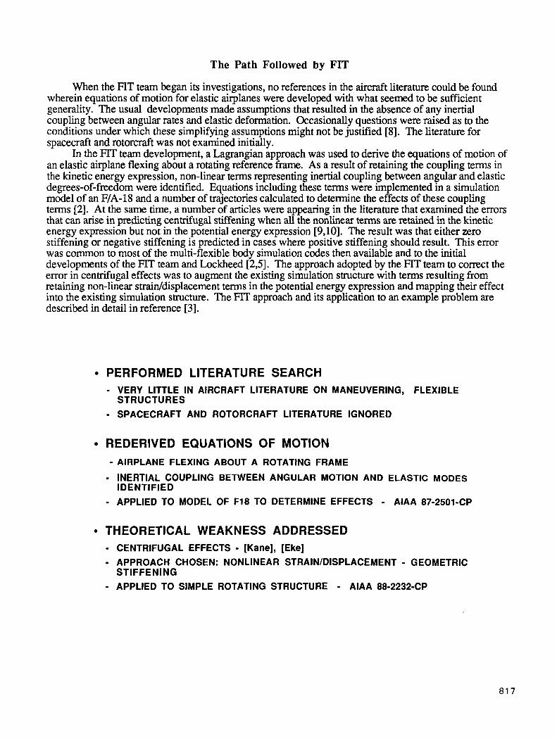
When the FIT team began its investigations, no references in the aircraft literature could be found wherein equations of motion for elastic airplanes were developed with what seemed to be sufficient generality. The usual developments made assumptions that resulted in the absence of any inertial coupling between angular rates and elastic deformation. Occasionally questions were raised as to the conditions under which these simplifying assumptions might not be justified [8]. The literature for spacecraft and rotorcraft was not examined initially.

In the FIT team development, a Lagrangian approach was used to derive the equations of motion of an elastic airplane flexing about a rotating reference frame. As a result of retaining the coupling terms in the kinetic energy expression, non-linear terms representing inertial coupling between angular and elastic degrees-of-freedom were identified. Equations including these terms were implemented in a simulation model of an F/A-18 and a number of trajectories calculated to determine the effects of these coupling terms [2]. At the same time, a number of articles were appearing in the literature that examined the errors that can arise in predicting centrifugal stiffening when all the nonlinear terms are retained in the kinetic energy expression but not in the potential energy expression [9,10]. The result was that either zero stiffening or negative stiffening is predicted in cases where positive stiffening should result. This error was common to most of the multi-flexible body simulation codes then available and to the initial developments of the FIT team and Lockheed [2,5]. The approach adopted by the FIT team to correct the error in centrifugal effects was to augment the existing simulation structure with terms resulting from retaining non-linear straiddisplacement terms in the potential energy expression and mapping their effect into the existing simulation structure. The FIT approach and its application to an example problem are described in detail in reference [3].

PERFORMED LITERATURE SEARCH - VERY LITTLE IN AIRCRAFT LITERATURE ON MANEUVERING, FLEXIBLE

STRUCTURES - SPACECRAFT AND ROTORCRAFT LITERATURE IGNORED

REDERIVED EQUATIONS OF MOTION - AIRPLANE FLEXING ABOUT A ROTATING FRAME

- INERTIAL COUPLING BETWEEN ANGULAR MOTION AND ELASTIC MODES IDENTIFIED

- APPLIED TO MODEL OF F18 TO DETERMINE EFFECTS - AlAA 87-2501-CP

THEORETICAL WEAKNESS ADDRESSED - CENTRIFUGAL EFFECTS - [Kane], [Eke]

STIFFENING - APPROACH CHOSEN: NONLINEAR STRAIN/DISPLACEMENT - GEOMETRIC

- APPLIED TO SIMPLE ROTATING STRUCTURE - AlAA 88-2232-CP

81 7

The Issues

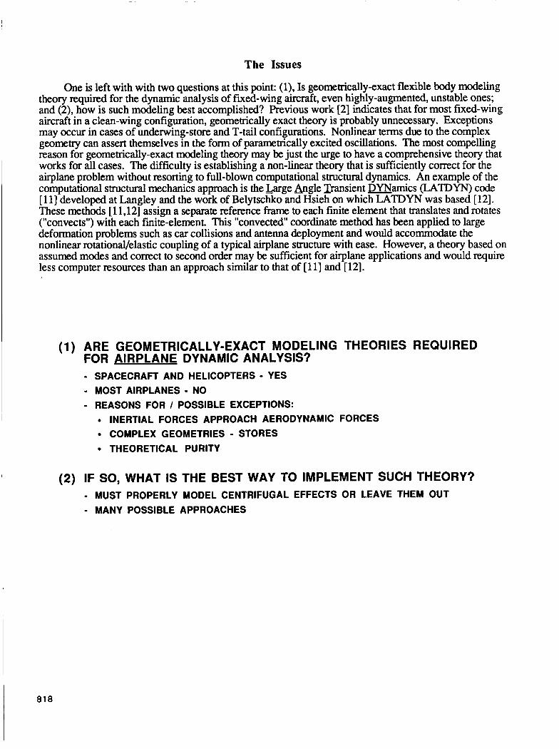
One is left with with two questions at this point: (l), Is geometrically-exact flexible body modeling theory required for the dynamic analysis of fixed-wing aircraft, even highly-augmented, unstable ones; and (2), how is such modeling best accomplished? Previous work [2] indicates that for most fixed-wing aircraft in a clean-wing configuration, geometrically exact theory is probably U M C X X S S ~ ~ ~ . Exceptions may occur in cases of underwing-store and T-tail configurations. Nonlinear terms due to the complex geometry can assert themselves in the form of parametrically excited oscillations. The most compelling reason for geometrically-exact modeling theory may be just the urge to have a comprehensive theory that works for all cases. The difficulty is establishing a non-linear theory that is sufficiently correct for the airplane problem without resorting to full-blown computational structural dynamics. An example of the computational structural mechanics approach is the M g e Angle Transient DYNamics (LATDYN) code [ 111 developed at Langley and the work of Belytschko and Hsieh on which LATDYN was based [ 121. These methods [ 1 1,121 assign a separate reference frame to each finite element that translates and rotates ("convects") with each finite-element. This "convected" coordinate method has been applied to large deformation problems such as car collisions and antenna deployment and would accommodate the nonlinear rotationaVelastic coupling of a typical airplane structure with ease. However, a theory based on assumed modes and correct to second order may be sufficient for airplane applications and would require less computer resources than an approach similar to that of [ll] and [12].

(1) ARE GEOMETRICALLY-EXACT MODELIP FOR AIRPLANE DYNAMIC ANALYSIS? - SPACECRAFT AND HELICOPTERS - YES - MOST AIRPLANES - NO - REASONS FOR / POSSIBLE EXCEPTIONS:

G Tt EORIES REQUIRED

INERTIAL FORCES APPROACH AERODYNAMIC FORCES COMPLEX GEOMETRIES - STORES THEORETICAL PURITY

(2) IF SO, WHAT IS THE BEST WAY TO IMPLEMENT SUCH THEORY? - MUST PROPERLY MODEL CENTRIFUGAL EFFECTS OR LEAVE THEM OUT - MANY POSSIBLE APPROACHES

818

Outline

The remainder of this paper is organized as follows. First the equations of motion are briefly described. Since an energy approach was taken in the development of the equations of motion [2,3], expressions for kinetic and potential energy are defined. The differences between the FlT model and the more typical aircraft aeroelastic equations [8,13] are explained. Prior to defining the the potential energy, a simple example [ 101 is presented to illustrate the notion of "geometric" stiffness. The higher order terms in the FIT potential energy expression are explained in light of the simple example. Once the equations are established, the effects of the including the nonlinear inertial coupling terms in the simulation model of an F/A-18 are presented. Time respnses due to a high-authority roll command are compared for the following cases: (l), additional terms mcluded; and (2), additional terms ignored. Finally, conclusions and recommendations are offered.

EQUATIONS OF MOTION

- KINETIC ENERGY - EXAMPLE OF GEOMETRIC STIFFNESS - POTENTIAL ENERGY

EFFECT OF INERTIAL LOADING - F/A-18

CONCLUSIONS

819

Modeling Assumptions

The operating assumptions in the equations of motion are listed below. Assumptions (2) through (4) are typical for airplane applications [8,13]. Assumptions (5) through (7) are atypical and lead to the differences between the FIT model and the more typical aeroelastic equations of motion [8,13].

The structural finite-element model obtained for the F/A- 18 was a lumped mass model, which provided the principal motivation for assumption (1). For a continuum model, summations over the lumped masses are replaced with integrations over the entire airplane. The finite-element model had both lumped masses and lumped inertial quantities and both were utilized in the calculations. Assumption (2) and (3) are consistent with each other. Assumption (2) leads to a generalized Hooke's law and assumption (3) allows the superposition of deformation modes. Assumption (4) reflects the fact that gravity grdients are only of concern in spacecraft dynamics.

Assumption (5 ) acknowledges that while defamation is assumed to be small, total vehicle angular rate may not be small. The result is that products of total angular rate and deformation rates are retained in the kinetic energy expression. The effect of assumption (6) is that the term resulting from summing (integrating) the cross product of deformation with deformation rates over the total vehicle is retained in the kinetic energy expression. Assumption (7) recognizes that a transverse deformation of a beam will result in axial strain. This effect becomes critical in correctly predicting centrifugal effects and is best explained in the simple example that appears later. Apart from assumptions (5), (6), and (7), the following development closely parallels other developments of the aeroelastic equations [8,13].

(1) LUMPED MASS APPROXIMATION

(2) LINEAR STRESS/STRAIN

(3) DEFORMATION IS SMALL - SUPERPOSITION

(4) GRAVITY CONSTANT OVER THE AIRPLANE

FOLLOWING ATYPICAL AEROELASTIC ASSUMPTIONS WERE MADE

(5) PRODUCTS OF ROTATION RATE AND DEFORMATION

(6) ELASTIC DISPLACEMENT AND ELASTIC VELOCITIES

ARE NOT NEGLIGIBLE

MAY NOT BE PARALLEL

(7) NON,LINEAR STRAIN / DISPLACEMENT

Symbols and Definitions

For the purposes of calculating kinetic energy, the total vehicle is viewed as a collection of small rigid bodies centered at the finite-element node locations. The lumped mass (dm)i and the lumped inertia

[dQi associated with the i- node can be interpreted as the result of performing integrations over the th

volume of the i l!l rigid body using s as a variable of integration and the mass density, 0, as a weighting function. The i h rigid body undergoes a translational deformation 4 and a rotational deformation 4. The assumption of small deformations allows the rotation to be described as a vector and implemented as a cross product. The vector 3 locates the undeformed position of the i- rigid body in the vehicle body frame. The origin of the body frame is at the center of mass of the total vehicle when the vehicle is in the undeformed configuration. The vector R locates an arbitrary point of the i' rigid body in the inertial frame.

th

......... .................., i REFERENCE POSITION OF

AIRPLANE CENTER OF

- r d i - THE RIGID MASS ELEMENT i CENTERED AT NODE i ........................... _ _ - - -

F MASS \d i

MASS ELEMENT AFTER ELASTIC DISPLACEMENT

...................................... - e ixs ,,, 1 0. 1

.....

s a . . 0 . .

* . I

- 0 . . a * .

0 MASS / UNIT VOLUME

r r r -

d K FIXED IN

INERTIAL FRAME

dm = JJJods i i

821

Total Kinetic Energy

.th The total kinetic energy is calculated in two steps. First the kinetic energy of the 1- rigid body (lumped mass) is found by performing the volume integration indicated in the brackets. The inertial velocity of an interior point is squared, multiplied by the mass density, 6, and integrated over the small rigid body. All volume integral expressions involving the variable,of integration 3 can be resolved into the "known" parameters, ( d n ~ ) ~ and [&Ii, that are defined in the previous figure .,A summauon is then perform& over the small rigid bodies indexed by i. Lf the deformations are described !s a sum of spatial functions ,(mode shapes) and time-dependent generalized coordinates, a separation of variables is achieved The kinetic energy becomes a summation of terms where each term is a product involving time varying coordinates and constant mass or length terms resulting from the summation (integration) over the total vehicle. '

INTEGRATE OVER THE IDEALIZED LUMPED MASS TO GET KINETIC ENERGY FOR EACH LUMPED MASS

SUM THE KINETIC ENERGIES ASSOCIATED WITH EACH LUMPED MASS

*............., WHERE

1 1 = P + r . + d * + S + @ S - e x s

1 1 i

I .i TRANSLATIONAL DEFORMATION i I IN MODAL COMPONENTS

d. 1 = gill

j ROTATIONAL DEFORMATION 1 II IN MODAL COMPONENTS

-. e = W"l l

d - dtI

TIME RATE OF CHANGE WITH RESPECT TO THE INERTIAL FRAME

I 822

Kinetic Energy in Modal Components

The first three terms of the expression defining kinetic energy, shown below, are found in the standard aeroelastic equations of motion developments [8,13] and represent "rigid" translational energy, "rigid" rotational energy, and elastic kinetic energy, respectively. The term [J,] is the inertia dyadic of the total undeformed airplane expressed in body-frame components and has units of mass- length . The fourth line describes coupling between translational, rotational, and elastic momenta. If the assumed mode shapes are the modes of free vibration of an unrestrained structure, they satisfy the first- order mean axis conditions [8,13] and the terms, a. and h. are zero. The term a. is simply the location of

the center of mass of the j' mode shape in the body frame and has units of length. The term h. is the first

moment of the J- mode shape in the body frame using mass as the weighting function and has units of mass-length2. The terms in the dashed-line box result from assumptions (5 ) and (6). The terms [J1. and [Jljk are the first and second partial derivatives of the inertia dyadic matrix with respect to elastic modes j and k. The term results from summing (integrating) the cross product of mode shape j with mode k

over the vehicle and has units of mass-length . For a more complete explanation, see reference 2.

2

3 3 -I

J . th

J

l?jk 2

T 3 m v . y RIGID BODY TRANSLATIONAL KINETIC ENERGY

+ TcU.[J,l 1 *o RIGID BODY ROTATIONAL KINETIC ENERGY

MODAL ELASTIC KINETIC ENERGY * j * k + L M q q

* j k

j + rnv.ajfij + o - h .fij + rny-oxa -J .q ZERO FOR UNRESTRAINED MODES - J

NONLlNEARlTlES RESULTING FROM ASSUMPTIONS (5), (6)

J

8 23

Illustration of Geometric Stiffness

The example shown below is taken from reference [lo] and provides a simple paradigm of the beam problem. Pictured is a simple 3 degree-of-freedom, planar system. A mass, m, is located at the outermost point and is the only mass in the system. The structure rotates freely about the point P. The angle between rod a and an inertial reference is given by yf. There is a torsional spring, kg, and a linear

spring, kb The deflection of the torsional spring is given by 8 and the linear spring by d = r6, where 6 is a nondimensional deflection. Another coordinate system (x,y) is given by an axis system located at the zero-strain position of the mass, m. The (x,y) coordinates are analogous to those typically used in the beam problem. The coordinates (c,q) are the non-dimensional forms of (x,y). Both the (v,S,8) and the (v,c,q) coordinate systems are equally valid for describing this system. The (yf,S,O) system leads to a particularly simple expression for strain energy. The reason is that a change in 6 produces only a linear distortion in the spring, ks, and similarly for 8. Thus the strain energy, U, is given by,

U = (1/2) ( k,e2 + k,62 )

2 where ks = kdr . The (v,t,q) system produces a complex expression for strain energy. A change in q produces nonlinear changes in both springs and similarly for 5 if there is some deflection in q. Using the relations,

6 = -1 + {q2+ (1+~)2)'/2 and 8 = Tan-'(q/(l+C)},

one gets for the strain energy, U, in terms of 5 and q,

TWO CHOICES FOR COORDINATES: ( W , 6 , e OR ( \I,, 5 , )

( 6 , e ) -> SIMPLE EXPRESSION FOR STRAIN ENERGY

( 5 , ~ ) -> COMPLEX STRAIN ENERGY EXPRESSION

PARADIGM OF BEAM PROBLEM

Comparison of Resulting Linear Models

If the full nonlinear equations are derived using the (v,S,O) coordinates, the v equation removed, -

and the quantities y~ and v are treated as parameters, the remaining two equations can be linearized in 8 and 6 and the resulting correct linear equations are given in case 1 below. Suppose the procedure is repeated for the (v,c,q) coordinates except that a linear approximation for strain energy given by,

is used, then the resulting equations are given as case 2 below [ 101. The only differences occur in the stiffness matrix. The foremost difference is that a de-stiffening result is predicted in case 2 for the q degree-of-freedom due to the spin rate when a stiffening effect should be predicted.

CASE I : Y AND k GIVEN; Y EQUATION REMOVED; LINEARIZED IN ti AND e

2 2 CASE 2: (6 ,ll ) COORDINATES; LINEAR STRAIN I DISPLACEMENT, U (1/2) { ke q + kti6 }

. 2 .. ABOVE kg - I , W

I = m r 2 I= = m a r r

8 25

Potential Energy

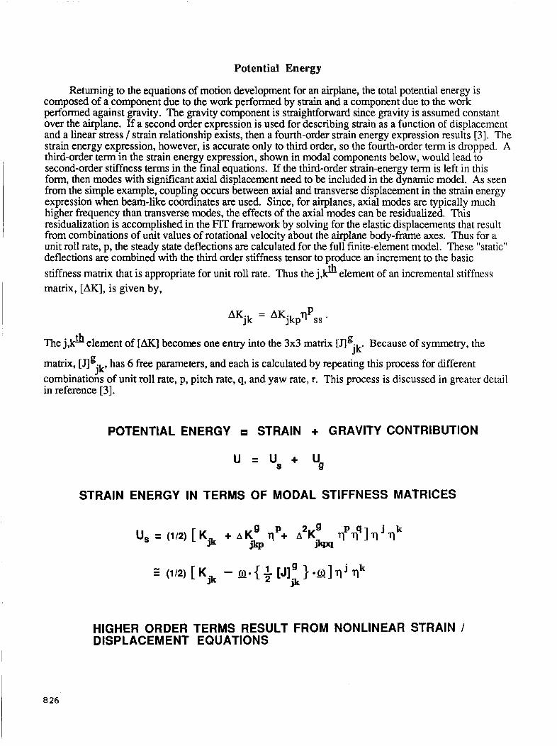
Returning to the equations of motion development for an airplane, the total potential energy is composed of a component due to the work performed by strain and a component due to the work performed against gravity. The gravity component is straightforward since gravity is assumed constant over the airplane. If a second order expression is used for describing strain as a function of displacement and a linear stress / strain relationship exists, then a fourth-order strain energy expression results [3]. The strain energy expression, however, is accurate only to third order, so the fourth-order term is dropped. A third-order term in the strain energy expression, shown in modal components below, would lead to second-order stiffness terms in the final equations. If the third-order strain-energy term is left in this form, then modes with significant axial displacement need to be included in the dynamic model. As seen from the simple example, coupling occurs between axial and transverse displacement in the strain energy expression when beam-like coordinates are used. Since, for airplanes, axial modes are typically much higher frequency than transverse modes, the effects of the axial modes can be residualized. This residualization is accomplished in the FIT framework by solving for the elastic displacements that result from combinations of unit values of rotational velocity about the airplane body-frame axes. Thus for a unit roll rate, p, the steady state deflections are calculated for the full finite-element model. These "static" deflections are combined with the third order stiffness tensor to produce an increment to the basic stiffness matrix that is appropriate for unit roll rate. Thus the j,k- element of an incremental stiffness th

I matrix, [AK], is given by,

The j,@ element of [AK] becomes one entry into the 3x3 matrix [Jlgjk Because of symmetry, the

matrix, [Jlgjk. has 6 free parameters, and each is calculated by repeating this process for different combinations of unit roll rate, p, pitch rate, q, and yaw rate, r. This process is discussed in greater detail in reference [3].

POTENTIAL ENERGY STRAIN + GRAVITY CONTRIBUTION

u = u + ug 8

STRAIN ENERGY IN TERMS OF MODAL STIFFNESS MATRICES

HIGHER ORDER TERMS RESULT FROM NONLINEAR STRAIN / DISPLACEMENT EQUATIONS

8 26

Final Equations - Unrestrained Modes

The final equations in modal form are shown below. These equations apply to the case where the assumed modes satisfy the first-order mean axis conditions, otherwise additional coupling is present. The terms that are inside the dashed boxes result from assumptions (3, (6), and (7). The terms outside the boxes are equivalent to the equations seen in the more traditional approaches [8,13].

TRANSLATIONAL MOMENTUM

ROTATIONAL MOMENTUM ......................... ............................................................................

ki 0 j ..k I - j -k + hjkq q : + a x [J ]a + [JIB+ h q q + axh q j i i = - L

-jk .ik ........................ ............................................................................ ELASTIC MODE j

........................................................................................................ .......................... ' 0 ki ki .k 1 k g k i I - o * h q i + K q :- 2 a . h q FW{[J]. + [J] ?l + [J] }ai= Qj - - * ; jk i -P J jk .ik

Mjkmik ............................ ........................................................................................................ !

TOTAL INERTIA MATRIX IN THE BODY FRAME ..........................................................................

.......................................................................... ,

8 27

Inertial Effects - Time History Responses

In assessing the effects of the additional terms in the FIT equations of motion on a predicted response, a variety of cases were calculated. While all three axes were examined, the most interesting responses involved roll rate. The responses shown here were presented at the 1987 Flight Simulation Technologies Conference [2] and were generated prior to the incorporation of the geomemc stiffness terms, [qgj,, in the simulation model. Preliminary runs made subsequently, but not presented in this paper, suggest that the effect of the additional stiffness terms is small for the angular rates cons ided and that qualitative conclusions drawn from the data presented in reference [2] a~ still valid.

The time responses were generated by injecting a roll command doublet at the actuator input. A combination of aileron and stabilator was used. The initial conditions were straight and level flight at Mach .7 at sea level. Responses were generated with ("terms on") and without ("terms off*) the additional anguladelastic coupling terms that are part of the FIT equations of motion.

8 28

GOAL: ACHIEVE SUFFICIENT ANGULAR RATE TO EXCITE INERTIAL RESPONSE

ROLL DOUBLET - 1 SECOND EACH SIDE

20 DEG AILERON / 10 DEG DIFFERENTIAL STABILATOR

INITIAL CONDITIONS

- MACH=.7

- SEA LEVEL

- STRAIGHT AND LEVEL 1 G TRIM

COMPARE RESPONSE WITH AND WITHOUT ANGULAR/ELASTIC INERTIAL COUPLING

- "TERMS ON" - FIT MODEL

- "TERMS OFF" - TYPICAL ASE MODEL

Lateral / Anti-Symmetric Response

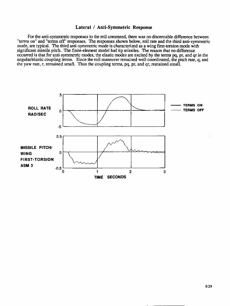
For the anti-symmetric responses to the roll command, there was no discernable difference between "terms on" and "terms off' responses. The responses shown below, roll rate and the third anti-symmetric mode, are typical. The third anti-symmetric mode is characterized as a wing first-torsion mode with significant missile pitch. The finite-element model had tip missiles. The reason that no difference occurred is that for anti-symmetric modes, the elastic modes are excited by the terms pq, pr, and qr in the angular/elastic coupling terms. Since the roll maneuver remained well-coordinated, the pitch rate, q, and the yaw rate, r, remained small. Thus the coupling terms, pq, pr, and qr, remained small.

0.5

ROLL RATE RAD/SEC

A - - MISSILE PITCH/ WING FIRST-TORSION ASM 3

- TERMS ON I,,.....,, TERMS OFF

TIME SECONDS

8 29

Symmetric Response - Set 1

5 -

0 '

The inertial coupling terms made no effect on rigid body symmetric responses. The angle-of-attack response is shown below. The angle-of-attack at time equal zero is due to the 1-g trim. The second response shown below is the first symmetric mode, wing first-bending. The y-axis indicates the deflection of the mode in feet measured at the point of maximum deflection, presumably at the wing tip. The mode is positive for tip-down deflection, so the mode is displaced about .25 feet tip-up at time zero. While the angle-of-attack is clearly the principal driver of symmetric wing first-bending in this maneuver, a discernable difference has occurred between the "terms on" and the "terms off'' responses. Only two symmetric modes showed more difference in "terms odoff' responses than the first symmetric mode and these two modes are shown in the f ipre on the next page.

- TERMS ON , , I I , I I I I I TERMS OFF a

DEG

WING FIRST- BENDING SYM 1

TIME SECONDS

Symmetric Response - Set 2

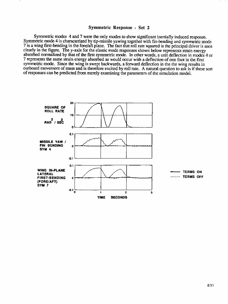
Symmetric modes 4 and 7 were the only modes to show significant inertially induced response. Symmetric mode 4 is characterized by tip-missile yawing together with fin-bending and symmetric mode 7 is a wing frrst-bending in the fore/aft plane. The fact that roll rate squared is the principal driver is seen clearly in the figure. The y-axis for the elastic mode responses shown below represents strain energy absorbed normalized by that of the first symmetric mode. In other words, a unit deflection in modes 4 or 7 represents the same strain energy absorbed as would occur with a deflection of one foot in the first symmetric mode. Since the wing is swept backwards, a forward deflection in the the wing results in outboard movement of mass and is therefore excited by roll rate. A natural question to ask is if these sort of responses can be predicted from merely examining the parameters of the simulation model.

SQUARE OF ROLL RATE

2 2 RAD I SEC

0.1 I 1 I I MISSILE YAW I FIN BENDING SYM 4

-0.1 I I J

0.1 I I 1 1 -okqLj-l WING IN-PLANE LATERAL FI RST-B ENDING (FOREIAFT) SYM 7

-0.1 0 1 2 3

TIME SECONDS

TERMS ON TERMS OFF

- I I I I I , , , . .

831

Modal Sensitivity Parameter

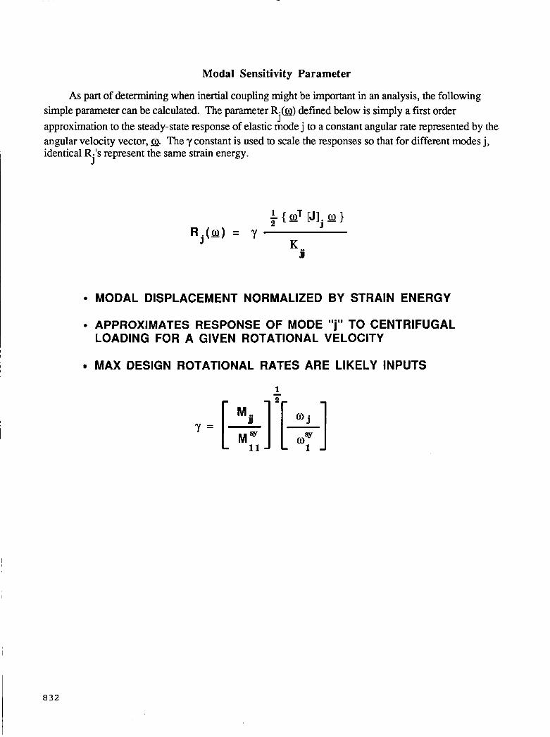
As part of determining when inertial coupling might be important in an analysis, the following simple parameter can be calculated. The parameter R.@) defined below is simply a first order

J approximation to the steady-state response of elastic mode j to a constant angular rate represented by the angular velocity vector, a. The y constant is used to scale the responses so that for different modes j, identical R.'s represent the same strain energy.

J

1 - 2 { cuT [JIj cu 1 Rj(cu) = y

K I

MODAL DISPLACEMENT NORMALIZED BY STRAIN ENERGY

APPROXIMATES RESPONSE OF MODE "j" TO CENTRIFUGAL LOADING FOR A GIVEN ROTATIONAL VELOCITY

MAX DESIGN ROTATIONAL RATES ARE LIKELY INPUTS

Modal Sensitivity at Max Roll

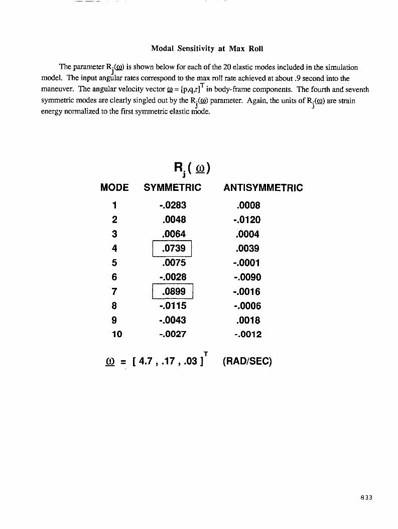
The parameter R . 0 is shown below for each of the 20 elastic modes included in the simulation J

model. The input angular rates correspond to the max roll rate achieved at about .9 second into the maneuver. The angular velocity vector symmetric modes are clearly singled out by the R.@) parameter. Again, the units of R.@) are strain energy normalized to the first symmetric elastic mode.

T = [p,q,r] in body-frame components. The fourth and seventh

J J

MODE

1 2 3 4 5 6 7 8 9 10

SYMMETRIC

-.0283 .0048 ,0064

I .0739 I .0075 -.0028

1 0 8 9 9 7 -.0115 -.0043 -.0027

T

ANTSY MMETRIC

,0008 -.0120 .0004 .0039 -.0001 -.0090 -.0016 -.0006 .0018 -.0012

- 0 = [ 4.7 , .I7 , .03 1' (RAD/SEC)

8 3 3

Illustration of R Parameter

The amplitudes of the response of symmetric modes 4 and 7 are essentially equal to the values of the R parameter calculated in the previous figure. This parameter, which is a linear approximation to steady-state response, is far from the end of the story. In the case of the FIT simulation model, even though symmetric modes 4 and 7 were excited by inertial effects, these modes are essentially decoupled from the rest of the dynamic model. This occurred because both modes 4 and 7 are dominated by in-plane bending of the wing lifting surface. A doublet-lattice code was used to calculate the generalized aerodynamic forces and in-plane motions produce no change in the normal washes induced at the 3/4 chord points of the aerodynamic boxes. Thus none of the other modes are significantly affected by symmetric modes 4 and 7.

One can imagine other cases where inertially affected modes are more coupled to the rest of the system dynamics. One case is if such a mode contributes to a feedback signal. Another case might occur in an underwing store configuration. As the underwing stores were slung outboard by centrifugal forces, they would induce out-of-plane bending in the wings, the primary lifting surfaces.

R4 ( ) = .074 AT MAX ROLL POINT

TERMS ON - MISSILE YAW I FIN BENDING II. I I I I I I I TERMS OFF SYM MODE 4

R,( 0) = .090 AT MAX ROLL POINT

WING IN-PLANE

FI RST-B EN DING LATERAL

(FOREIAFT) SYM MODE 7

-0.1 0 1 2 3

TIME SECONDS

8 34

Conclusion

An integrated, nonlinear simulation model suitable for aeroelastic modeling of fixed-wing aircraft has been developed. While the author realizes that the subject of modeling rotating, elastic structures is not closed, it is believed that the equations of motion developed and applied herein are correct to second order and are suitable for use with typical aircraft structures. The equations are not suitable for large elastic deformation. In addition, the modeling framework generalizes both the methods and terminology of non-linear rigid-body airplane simulation and traditional linear aeroelastic modeling.

Concerning the importance of angular/elastic inertial coupling in the dynamic analysis of fixed-wing aircraft, the following may be said. The rigorous inclusion of said coupling is not without peril and must be approached with care. In keeping with the same engineering judgment that guided the development of the traditional aeroelastic equations, the effect of non-linear inertial effects for most airplane apphcations is expected to be small. A parameter has been presented to help in the determination of when such effects are significant. The parameter does not tell the whole story, however, and modes flagged by the parameter as significant also need to be checked to see if the coupling is not a one-way path, i.e. the inertially affected modes can influence other modes. Classically, configurations where nonlinear inertial effects can come into play are characterized by complex geometries such as stores mounted under the wings or the presence of a T-tail.

INTEGRATED NONLINEAR MODEL DEVELOPED - CORRECT TO SECOND ORDER - SUITABLE FOR AIRPLANE STRUCTURES

GENERALIZES CONVENTIONAL ASE MODELS AND NONLINEAR RIGID-BODY MODELS

ANGULAR / ELASTIC INERTIAL COUPLING - RIGOROUS INCLUSION PROBLEMATIC - - EXCEPTIONS CHARACTERIZED BY

EFFECT NORMALLY SMALL FOR AIRPLANES

R ( Q ) PARAMETER IS SIGNIFICANT FOR SOME MODE

- AND AFFECTED MODE IS COUPLED TO THE REST OF THE MODEL

835

REFERENCES

1. Hood, R.V.; Dollyhigh, S.M.; and Newsom,J.R.: Impact of Flight Systems Integration on Future Aircraft Design. AIAA Paper 85-1865, August 1985.

2. Buttrill, C.S.; Zeiler, T.A.; and Arbuckle, P.D.: Nonlinear Simulation of a Flexible Aircraft in Maneuvering Flight. AIAA Paper 87-2501-CP. AIAA Flight Simulation Technologies Conference (Monterey, CA), August 1987.

3. Zeiler, T.A.; and Buttrill, C.S.: Dynamic Analysis of an Unrestrained, Rotating Structure Through Nonlinear Simulation. AIAA Paper 88-2232-CP. AIAA/ASME/ASCE/AHS 29th Structures, Structural Dynamics and Materials Conference (Williamsburg, VA), April 1988.

4. Arbuckle, P.D.; Buttrill, C.S.; and Zeiler,T.A.: A New Simulation Model Building Technique For Use In Dynamic Systems Integration Research. AIAA Paper 87-2498-CP. AIAA Flight Simulation Technologies Conference (Monterey, CA), August 1987.

Youssef, H.M.; Nayak, A.P.; and Gousman, K.G.: Integrated Total Flexible Body Dynamics of Fixed Wing Aircraft. AIAA Paper 88-2364-CP. AIAA/ASME/ASCE/AHS 29th Structures, Structural Dynamics and Materials Conference (Williamsburg, VA), April 1988.

6. Morino, L.; and Baillieul, J.: A Geometrically-Exact Non-Linear Lagrangian Formulation for the Dynamic Analysis of a Flexible Maneuvering Airplane. Prepared for the USAF Office of Scientific Research, Contract F49620-86-C-0040. Center for Computational and Applied Dynamics, Boston University, CCAD-TR-87-02.

7. Likens,P.W.: Dynamics and Control of Flexible Space Vehicles. NASA Technical Report 32-1329. Jet Propulsion Laboratory, Pasadena, CA. February 15, 1969.

8. Cavin, R.K.; and Dusto, A.R.: Hamilton's Principle: Finite-Element Methods and Flexible Body Dynamics. AIAA Journal, vol. 15, no. 12, December 1977, pp. 1684-1690.

9. Kane, T.R.; Ryan, R.R.; and Bannerjee: Dynamics of a Cantilever Beam Attached to a Moving Base. AIAA Journal of Guidance, Control, and Dynamics, vol. 10, no. 2, Mar-Apr 1987, pp.

10. Eke, F.O.; and Laskin, R.A.: On the Inadequacies of Current Multi-Flexible Body Simulation Codes. AIAA Paper 87-2248-CP. AIAA Guidance, Navigation and Control Conference (Monterey, CA), August 1987.

1 1. Housner, J.M.; McGowan, P.E.; Abrahamson, A.L.; and Powell, M.G.: The LATDYN User's Manual. NASA TM 87635, 1986.

12. Belytschko, T; and Hsieh, B.J.: Non-Linear Transient Finite Element Analysis With Convected Co- Ordinates. International Journal for Numerical Methods in Engineering, vol. 7, 1973, pp. 255- 272.

13. Waszak,M.; and Schmidt,D.K.: Flight Dynamics of Aeroelastic Vehicles. AIAA Journal of Aircraft, vol. 25, no. 6, June 1988, pp 563-571.

5 .

139- 15 1.