71

CHAPTER 3 Cardiovascular Responses

The heart, consequently, is the beginning of life, the sun of the microcosm, even as the sun in his turn might be designated the heart of the world; for it is the heart by whose virtue and pulse the blood is moved, perfected, made apt to nourish, and is perceived from corruption and coagulation: it is the household divinity which, discharging its function, nourishes, cherishes, quickens the whole body, and is indeed the foundation of life, the source of all action. - William Harvey

3.1 INTRODUCTION The purpose of the cardiovascular system is primarily to supply oxygen and remove carbon dioxide from metabolizing tissues.1 Perhaps this is the reason for the almost immediate cardiac response to the beginning of exercise when the metabolic needs of the muscles increase dramatically. Indeed, cardiovascular responses are so rapid that the severity of exercise stress is usually judged on the basis of an instantaneous heart rate sample. A second important cardiovascular function during exercise is removal of excess heat (see Chapter 5). Vasodilation of surface blood vessels brings warm blood in closer contact with the cool air to facilitate heat transfer. This response does not occur at all rapidly, however. Due to the thermal mass of the body, 10-15 minutes may elapse between the start of exercise and active vasodilatory responses. There are times when the chemical transport and heat transport functions of the blood come into direct conflict, since blood required for supply of skeletal muscle needs may be shunted to the skin for heat removal. When this happens, muscle metabolism must become at least partially anaerobic. Since there is a limit to the amount of anaerobic metabolism that can occur, this conflict can directly lead to a shortened exercise period. It is the purpose of this chapter to detail cardiovascular mechanics and control during exercise. This book considers four elements of the cardiovascular system: the heart, the vasculature, respiratory interface, and thermal interface. Respiratory interface is treated in Chapter 4 and thermal interface in Chapter 5. 3.2 CARDIOVASCULAR MECHANICS The cardiovascular mechanical system is composed of blood, vessels which contain the blood, and the heart to pump the blood through the vessels. In addition, the system contains substances to repair rupture. 1Because the blood permeates the entire body, it also performs a useful humoral communication function. is important in assisting transport and removal of chemical metabolites, and is useful in the body's defense against disease.

72

3.2.1 Blood Characteristics Blood composition is very complex, and much beyond the scope of this book. There are, however, physical properties of the blood which are of concern to bioengineers and exercise physiologists. Composition. A general classification separates blood into red blood cells, white blood cells, and plasma. Blood cells constitute 45% of total blood volume and plasma 55% (Ganong, 1963). Circulating blood2 contains an average of 5.4 x 1015 red blood cells per cubic meter in men and 4.8 x 1015 per cubic meter in women (Ganong, 1963). + Oxygen-Carrying Capacity. Oxygen is transported by the blood by two different, but complementary mechanisms: as oxygen dissolved in the blood plasma and as oxygen chemically united with hemoglobin in the red blood cells (Table 3.2.1). Each human red blood cell contains approximately 29 pg (picograms) of hemoglobin. The body of a 70 kg man contains about 900 g of hemoglobin and that of a 60kg woman, about 660g (Ganong, 1963). Each hemoglobin molecule contains four heme units, each of which can bind with one oxygen molecule (i.e., diatomic oxygen, O2). When fully saturated, each kilogram of hemoglobin contains 1.34 x 10-3 m3, (1.34mL O2/g) (Ganong, 1963). Since average men have about 160 kilograms hemoglobin per cubic meter of blood (160g/L blood), 0.214 m3 O2/m3 blood (214mL O2/L blood) is bound by their hemoglobin. The amount of oxygen which is physically and passively dissolved in the blood plasma is usually expressed in terms of partial pressure. The partial pressure of a gas is defined as that pressure which would exist in the gas for the free gas to be in equilibrium with the gas in solution. The higher the partial pressure exerted by a gas above a solution, the more gas will dissolve in solution. For respiratory oxygen, the number of cubic meters of gas dissolved in one cubic meter of blood at 38ºC at a partial pressure of one atmosphere (1 atm, 105 N/m2) and with gas volume corrected to conditions of standard temperature and pressure ,3 called the Bunsen coefficient, is 0.023 (Mende, 1976). For example, if the percentage of oxygen in the alveolus is 12%, expressed as dry gas, then the percentage of oxygen, taking into account that alveolar air is saturated with water vapor, is

( ) %2.11%)12(N/m10

N/m62661025

25=

−

The partial pressure of oxygen4 therefore is pO2 = (11.2/100)(105 N/m2) = 11.2 x 103 N/m2 (3.2.1) and the amount of oxygen dissolved5 in the pulmonary venous blood is

2OV =

5

3

1010x2.11 (0.023) = 0.00258 m3O2 / m3 blood (2.58mL O2 /L blood) (3.2.2)

2The ratio of circulating blood volume, expressed as cubic centimeters, to body mass, expressed in kilograms, is about 80. 3Standard temperature and pressure are OºC and 1 atm (760 mm Hg, or 105 N/m2). Furthermore,. respiratory gases are usually expressed as dry gas and 6266 N/m2 (47 mm Hg) is subtracted from total atmospheric pressure to account for water vapor in lung gases. 4Normal arterial pCO2 is 5.3 kN/m2 (40 mm Hg) and normal arterial pO2 is 13.3 kN/m2 (100 mm Hg). 5The amount of O2 in mL per 100 mL of blood in a particular sample is usually designated by physiologists as the O2 content of the blood. For purposes of unit consistency, we use (m3 O2/m3 blood). To convert (m3 O2/m3 blood) to (mL O2/100 mL blood), multiply (m3 O2/m3 blood) by 100.

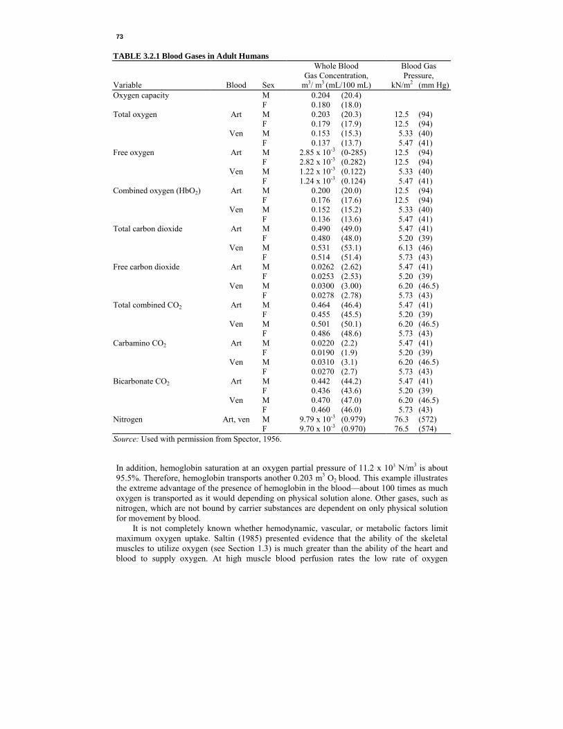
73

TABLE 3.2.1 Blood Gases in Adult Humans Whole Blood Blood Gas Gas Concentration, Pressure, Variable Blood Sex m3/ m3 (mL/100 mL) kN/m2 (mm Hg) Oxygen capacity M 0.204 (20.4) F 0.180 (18.0) Total oxygen Art M 0.203 (20.3) 12.5 (94) F 0.179 (17.9) 12.5 (94) Ven M 0.153 (15.3) 5.33 (40) F 0.137 (13.7) 5.47 (41) Free oxygen Art M 2.85 x 10-3 (0-285) 12.5 (94) F 2.82 x 10-3 (0.282) 12.5 (94) Ven M 1.22 x 10-3 (0.122) 5.33 (40) F 1.24 x 10-3 (0.124) 5.47 (41) Combined oxygen (HbO2) Art M 0.200 (20.0) 12.5 (94) F 0.176 (17.6) 12.5 (94) Ven M 0.152 (15.2) 5.33 (40) F 0.136 (13.6) 5.47 (41) Total carbon dioxide Art M 0.490 (49.0) 5.47 (41) F 0.480 (48.0) 5.20 (39) Ven M 0.531 (53.1) 6.13 (46) F 0.514 (51.4) 5.73 (43) Free carbon dioxide Art M 0.0262 (2.62) 5.47 (41) F 0.0253 (2.53) 5.20 (39) Ven M 0.0300 (3.00) 6.20 (46.5) F 0.0278 (2.78) 5.73 (43) Total combined CO2 Art M 0.464 (46.4) 5.47 (41) F 0.455 (45.5) 5.20 (39) Ven M 0.501 (50.1) 6.20 (46.5) F 0.486 (48.6) 5.73 (43) Carbamino CO2 Art M 0.0220 (2.2) 5.47 (41) F 0.0190 (1.9) 5.20 (39) Ven M 0.0310 (3.1) 6.20 (46.5) F 0.0270 (2.7) 5.73 (43) Bicarbonate CO2 Art M 0.442 (44.2) 5.47 (41) F 0.436 (43.6) 5.20 (39) Ven M 0.470 (47.0) 6.20 (46.5) F 0.460 (46.0) 5.73 (43) Nitrogen Art, ven M 9.79 x 10-3 (0.979) 76.3 (572) F 9.70 x 10-3 (0.970) 76.5 (574) Source: Used with permission from Spector, 1956.

In addition, hemoglobin saturation at an oxygen partial pressure of 11.2 x 103 N/m3 is about 95.5%. Therefore, hemoglobin transports another 0.203 m3 O2 blood. This example illustrates the extreme advantage of the presence of hemoglobin in the blood—about 100 times as much oxygen is transported as it would depending on physical solution alone. Other gases, such as nitrogen, which are not bound by carrier substances are dependent on only physical solution for movement by blood. It is not completely known whether hemodynamic, vascular, or metabolic factors limit maximum oxygen uptake. Saltin (1985) presented evidence that the ability of the skeletal muscles to utilize oxygen (see Section 1.3) is much greater than the ability of the heart and blood to supply oxygen. At high muscle blood perfusion rates the low rate of oxygen

74

extraction related to the low mean transit time of blood passing through the capillaries. Enlargement of muscular capillary beds which accompanies endurance training probably serves the purpose of lengthening the mean transit time, not necessarily to increase blood flow.6 The presence of hemoglobin in the blood thus tends to narrow the gap between oxygen supply capacity and oxygen utilization capacity. Oxygen bound to hemoglobin is in equilibrium with oxygen in plasma solution. When oxygen is removed from hemoglobin, it first passes into the plasma as dissolved oxygen before it is made available to the tissues. When oxygen is added to hemoglobin, it comes from alveolar tissue by way of solution in the plasma. It is natural, therefore, that the oxygen-carrying capacity of hemoglobin be expressed in terms of oxygen partial pressure of the surrounding plasma. Typical oxygen dissociation curves with their characteristic sigmoid shapes are seen in Figures 3.2.1 through 3.2.3. Blood is very well buffered to minimize sudden changes in its chemical and physical structure. The hemoglobin saturation curve does shift, however, in response to changes of pCO2 (Figure 3.2.1),7 pH (Figure 3.2.2),8 and temperature (Figure 3.2.3). All of these are important in compensation for the oxygen demands of exercising muscle. Figure 3.2.1 shows the direct effect of carbon dioxide on hemoglobin dissociation. For any given level of oxygen partial pressure, an increase in plasma carbon dioxide reduces the equilibrium hemoglobin saturation. Oxygen is thus removed from each hemoglobin molecule and either increases dissolved oxygen or moves to the respiring tissues. Since carbon dioxide is produced most in regions with high oxygen demand, this hemoglobin saturation shift makes extra oxygen available where it is most needed. In the muscles, this extra oxygen is stored by myoglobin (see Section 1.3.2), a molecule with function similar to hemoglobin, for use as needed by muscle cells. When excess carbon dioxide is added to the venous blood, an important blood bicarbonate ( −

3HCO ) buffering system minimizes changes to the blood and allows higher carbon dioxide-carrying capacity. This buffering occurs by means of the following reversible chemical reactions (Ganong, 1963):

−+ +⇔⇔+ 33222 HCOHCOHCOOH (3.2.3) As carbon dioxide is added to the blood, it combines with plasma water to form a weak acid, carbonic acid. This dissociates into hydrogen ions and blood bicarbonate. At the lungs these reactions are reversed and blood bicarbonate is reduced as carbon dioxide is expelled. Carbon dioxide production also changes acidity of the blood, as measured by pH9, which also affects the hemoglobin saturation curve (Figure 3.2.2). The Henderson-Hasselbalch 6However, Saltin also adds that the capacity of the muscles to receive blood flow exceeds by a factor of 2 to 3 the capacity of the heart to supply the flow. Because of this, arterioles feeding the muscles must normally be subject to a vasoconstrictive neural control. 7Reduced hemoglobin is a weak acid. When combined with oxygen, hemoglobin (Hb) undergoes the chemical process which

+− +⇔⇔+ HHbOHHbOHHbO 222

makes additional hydrogen ions available to drive the carbon dioxide dissociation equilibrium (Equation 3.2.3) to the left. Thus increased oxygen saturation of the hemoglobin is accompanied by increased availability of carbon dioxide. This process is called the Haldane effect (Tazawa et al., 1983). 8Hemoglobin has a high buffering capacity over the normal range of blood pH. Without this buffering capacity. blood pH would vary greatly as blood carbon dioxide content changed. As CO2 is added to the blood, pH falls. With a fall in blood pH, oxygen is released from the hemoglobin molecule. This interaction between blood pH and oxygen saturation is called the Bohr effect. 9pH is defined as the negative logarithm of the hydrogen ion concentration. As the blood becomes more acid, hydrogen ion concentration increases and pH decreases.

75

Figure 3.2.1 Effect of blood carbon dioxide on the oxygen dissociation curve of whole blood. CO2 partial pressure for each curve is given in N/m2 (mm Hg). An increase in CO2 causes blood of a given oxygen saturation to increase the pO2, thus making O2 more readily available to dissolve in the plasma and transfer to surrounding tissues. Normal pCO2 is taken to be 5330 N/m2 (40mm Hg). (Adapted and used with permission from Barcroft, 1925.)

equation (Woodbury, 1965) relates pH to the buffering system of Equation 3.2.3:

pH = 6.10 x

−

32

3

COH

HCOlogc

c (3.2.4)

where cX = concentration of constituent X, mol/m3 Normal

32-3

COHHCO / cc ratio is 20 and normal arterial blood pH level is 7.4 (Ganong, 1963).

As long as blood oxygen levels can supply all the necessary oxygen required by exercising muscles, there is a direct correspondence between blood pH and CO2 produced by metabolism. When metabolism becomes nonaerobic. and lactic acid is a product of incomplete metabolism (see Section 1.3.2), an increase in hydrogen ion concentration occurs, blood pH lowers, and blood pCO2 rises. The equilibrium oxygen hemoglobin saturation curve indicates that further oxygen is then made available to the muscles. Aberman et al. (1973) presented an equation for the oxygen hemoglobin dissociation curve which is mathematically derived and can be useful for calculation purposes:

Sstd =

+−

∑= 6663.3O

6663.3O

std2

std27

0 pp

Ci

i (3.2.5)

where Sstd = oxygen saturation for standard conditions, % Ci = coefficients, %

76

Figure 3.2.2 Effect of blood acidity level on the oxygen dissociation curve of whole blood. Blood pH is given for each curve. As blood becomes more acid, its pH falls and blood pO2 rises for any given level of hemoglobin saturation. Thus O2 is made more readily available to dissolve in the plasma and be transferred to surrounding tissues. Normal blood pH is usually taken to be 7.40. (Adapted and used with permission from Peters and Van Slyke, 1931.)

Figure 3.2.3 Effect of blood temperature on the oxygen dissociation curve of whole blood. Blood temperature is indicated on each curve. As temperature rises, blood pO2 rises for any given saturation level. Thus O2 is more readily available for solution in the plasma and to surrounding tissues. Normal body temperature is 37ºC. (Adapted from Roughton, 1954.)

77

pO2std = partial pressure of oxygen of the standard dissociation curve, kN/m2

C0 = +51.87074 C1 = +129.8325 C2 = +6.828368 C3 = –223.7881 C4 = –27.95300 C5 = +258.5009 C6 = +21.84175 C7 = –119.2322 If pO2 is measured at any conditions other than the standard temperature of 37ºC, pH of 7.40, and base excess10 of 0 Eq/m3, a correction must be applied:

Sact = Sstd[10[0.024(37 – θ)] – 0.48 (7.40 – pH) – 0.0013B) (3.2.6) where Sact = actual saturation percentage θ = temperature, ºC B = base excess, Eq/m3 (Eq = charge equivalents) Equation 3.2.5 fits only the standard oxygen hemoglobin dissociation curve with a pO2 at 50% saturation of 3.546 kN/m2 (26.6 mm Hg). It is not accurate below a pO2, of 253 N/m2 (1.9 mm Hg) or above a pO2, of 93.3 kN/ m2 (700 mm Hg) and should not be used to predict saturation when pulmonary shunts, cardiac output, or arterial-venous oxygen content differences are calculated (Aberman et al., t973). Hemoglobin in the red blood cells is also involved in transport of carbon dioxide (Kagawa, 1984; Mochizuki et al., 1985). Carbon dioxide reacts with amino groups, principally hemoglobin, to form carbamino compounds. Reduced hemoglobin (that which has released its oxygen and taken up more hydrogen ions) forms carbamino compounds much more readily than oxyhemoglobin (Ganong, 1963). Thus transport of carbon dioxide is facilitated in venous blood (Figure 3.2.4).

Figure 3.2.4 CO2 titration curve of whole blood. Note that oxygenated blood contains less CO2 than reduced blood. Blood goes through a cycle, as indicated by A (arterial blood) and V (venous blood) in the capillaries of tissues and lungs. (Adapted and used with permission from Peters and Van Slyke, 1931.) 10Base excess refers to the bicarbonate concentration in Equation 3.2.3 and varies directly as pCO2.

78

From Table 3.2.1, we can see that male arterial blood carries a total of 0.490 m3 CO2/m3

blood. Of these, 0.026 m3 CO2/m3 blood is in free solution and 0.464 m3 CO2/m3 blood is combined in some way. Of the combined CO2, .022 m3 CO2/m3 blood is transported as carbamino compounds and 0.442 m3 CO2/m3 blood is transported as bicarbonate. Viscosity. Aside from the physicochemical characteristics of blood already described, blood must also be considered in light of its flow characteristics through the blood vessels. Since blood is a homogeneous substance from only the coarsest perspective, it cannot be expected to behave quite like truly homogeneous fluids such as water and oil. The most important flow characteristic of blood is its viscosity, which is a measure of its resistance to motion. If two plates containing a thickness r of fluid between them are drawn apart by a force F at rate v (Figure 3.2.5), then the force F divided by the plate area A is defined as the shear stress τ = F/A, and the rate of shear is defined as γ = dv/dr. Shear stress is related

Figure 3.2.5 Conceptual apparatus for determining fluid rheological properties.

Figure 3.2.6 Fluid rheological characteristics.

79

to the force required to pump a fluid through a tube, and the rate of shear is related to the rate at which the fluid flows. The ratio of shear stress to rate of shear is given the name viscosity:

µ = drdvAF

//

γ=τ (3.2.7)

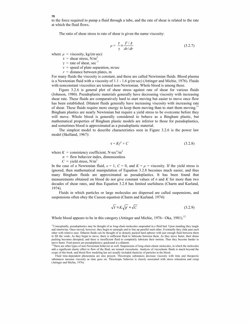
where µ = viscosity, kg/(m·sec) τ = shear stress, N/m2 γ = rate of shear, sec–1 v = speed of plate separation, m/sec r = distance between plates, m For many fluids the viscosity is constant, and these are called Newtonian fluids. Blood plasma is a Newtonian fluid with a viscosity of 1.1 - 1.6 g/(m·sec) (Attinger and Michie, 1976). Fluids with nonconstant viscosities are termed non-Newtonian. Whole blood is among these. Figure 3.2.6 is general plot of shear stress against rate of shear for various fluids (Johnson, 1980). Pseudoplastic materials generally have decreasing viscosity with increasing shear rate. These fluids are comparatively hard to start moving but easier to move once flow has been established. Dilatent fluids generally have increasing viscosity with increasing rate of shear. These fluids require more energy to keep them moving than to start them moving.11 Bingham plastics are nearly Newtonian but require a yield stress to be overcome before they will move. Whole blood is generally considered to behave as a Bingham plastic, but mathematical properties of Bingham plastic models are inferior to those for pseudoplastics, and sometimes blood is approximated as a pseudoplastic material. The simplest model to describe characteristics seen in Figure 3.2.6 is the power law model (Skelland, 1967): τ = Kγn + C (3.2.8) where K = consistency coefficient, N·secn/m2 n = flow behavior index, dimensionless C = yield stress, N/m2 In the case of a Newtonian fluid, n = 1, C = 0, and K = µ = viscosity. If the yield stress is ignored, then mathematical manipulation of Equation 3.2.8 becomes much easier, and thus many Bingham fluids are approximated as pseudoplastics. It has been found that measurements obtained on blood do not give constant values of n and K for more than two decades of shear rates, and thus Equation 3.2.8 has limited usefulness (Charm and Kurland, 1974). Fluids in which particles or large molecules are dispersed are called suspensions, and suspensions often obey the Casson equation (Charm and Kurland, 1974): CK += γτ (3.2.9) Whole blood appears to be in this category (Attinger and Michie, 1976~ Oka, 1981).12 11Conceptually, pseudoplastics may be thought of as long-chain molecules suspended in a fluid bed. Upon standing they tangle and intertwine. Once moved, however, they begin to untangle and to line up parallel each other. Eventually they slide past each other with relative ease. Dilatent fluids can be thought of as densely packed hard spheres with just enough fluid between them to fill the voids. As they begin to move, there is sufficient fluid to lubricate between them. As they move faster, their dense packing becomes disrupted, and there is insufficient fluid to completely lubricate their motion. Thus they become harder to move faster. Fruit purees are pseudoplastics; quicksand is a dilatent. 12There are other types of non-Newtonian behavior as well. Suspensions of long-chain elastic molecules, in which the molecules add a significant elastic effect to flow of the fluid, are termed viscoelastic. Analysis of viscoelastic fluids is much beyond the scope of this book, and blood flow modeling has not usually included elasticity of particles in the blood. Fluid time-dependent phenomena are also present. Thixotropic substances decrease viscosity with time and rheopectic substances increase viscosity as time goes on. Thixotropic behavior is closely associated with stress relaxation and creep (Attinger and Michie, 1976).

80

Figure 3.2.7 Viscosity-shear rate relationships of reconstituted blood from 37 to 22ºC. Hematocrits of the curves in each plot are 80% (top), 60%, 40%, 20%, and 0% (bottom). The axis labeled viscosity is actually the slope of the shear stress-rate of shear diagram (Figure 3.2.6). Since viscosity appears to be higher at low rates of shear, these measurements confirm whole blood to be a pseudoplastic substance tending to Newtonian as hematocrit decreases. (Adapted and used with permission from Rand et al., 1964.) At shear rates greater than 100 sec–1 normal blood behaves as a Newtonian fluid (Attinger and Michie, 1976; Haynes and Burton, 1959; Pedley et al., 1980) with a viscosity of 4–5 g/(m·sec) (Attinger and Michie, 1976). This value decreases by 2-3% per degree Celsius rise in temperature (Attinger and Michie. 1976). As hematocrit13 increases, apparent viscosity increases nonlinearly (Figure 3.2.7). Because red blood cells deform so easily, blood exhibits about half the viscosity of a suspension of similarly sized and distributed hard spheres in plasma (Attinger and Michie, 1976). Exercising individuals exhibit a so-called plasma shift due to body fluid losses mostly as sweat. Plasma volume decreases during exercise, thus concentrating suspended materials. This hemoconcentration averages less than 2% below exercise levels requiring 40% of maximum oxygen uptake (see Section 1.3); above 40% of maximum oxygen uptake hemoconcentration is 13Hematocrit is defined as the ratio of red blood cell volume to total blood volume, in percent. Hematocrit is usually determined by centrifugal separation. Hematocrit may vary from one vascular bed to another, where microvessels generally have lower hematocrit than their supply vessels. Fluid near the wall of blood vessels usually contains fewer red blood cells than the fluid in the center (Attinger and Michie, 1976). Hematocrit for men is usually about 0.47 and for women and children is 0.42 (Astrand and Rodahl, 1970).

81

directly proportional to work rate (Senay, 1979). Transient plasma volume decreases of 6–12% with the onset of exercise are corrected within 10–20 min after exercise ceases. Acclimation (see Section 5.3.5) to work in the heat is accompanied by a chronic hematocrit decrease as plasma volume increases. 3.2.2 Vascular Characteristics Blood vessels serve the purposes of blood transport, filtering of pressure extremes, regulation of blood pressure, chemical exchange, and blood storage. They generally are classified as arteries, arterioles, capillaries, and veins, each with different storage, elastic, and resistance properties (Table 3.2.2). Organization. The arteries are the first vessels encountered by the blood as it leaves the heart. Arteries are large-diameter vessels with very elastic walls. The large interior diameter allows a high volume of stored blood and the elastic walls store energy during heart contraction (systole) and release it between contractions (diastole). Thus the arteries play an important role in converting an intermittent blood delivery into a continuous one. Arterioles are smaller vessels with less elastic walls containing transversely oriented TABLE 3.2.2 Characteristics of Various Types of Blood Vessels Approximate Total Percentage of Lumen Wall Cross-Sectional Blood Volume Variable Diameter Thickness Area Containeda

Aorta 2.5 cm 2mm 4.5 cm2 2% Artery 0.4 cm 1 mm 20 cm2 8% Arteriole 30 µm 20 µm 400 cm2 1% Capillary 6 µm 1 µm 4500 cm2 5% Venule 20 µm 2 µm 4000 cm2 Vein 0.5 cm 0.5 mm 40 cm2 {50%} Vena cava 3 cm 1.5 mm 18 cm2 Source: Used with permission from Ganong, 1963. aOf the remainder, about 20% is found in the pulmonary circulation and 14% in the heart (Attinger, 1976a).

TABLE 3.2.3 Distribution of Blood to Various Organs for a Normal 70 Kg (685 N) Man at Rest Percentage of Total Blood Blood Variable Weight Volume Flow O2 Consumption Muscle 41.0 10.0 17.0 21.0 Skin 5.0 1.5 7.0 6.0

4.0 23.0 27.0 22.0 Gastrointestinal tract Brain 2.5 0.5 13.0 8.5 Kidney 1.0 2.0 26.0 8.0 Heart 0.5 0.5 5.0 12.5 Othera 46.0 62.5 5.0 22.0 100.0% 100.0% 100.0% 100% Nominal total 685 N 5600 cm3 (5.6 L) 92 cm3/sec(5.5 L/min) 4.2cm3/sec(250 mL/min) Source: Used with permission from Michie et al., 1976. aBone, fat, connective tissue, pulmonary circulation, heart chambers, larger peripheral arteries and veins.

82

TABLE 3.2.4 Changes in Blood Distribution to Various Organs Between Rest and Exercise Variable Rest Exercise Actual Change Lungs 100% 100% ++ Gastrointestinal tract 25–30 3–5 – Heart 4–5 4–5 ++ Kidneys 20–25 2–3 — Bone 3–5 0.5–1 + Brain 15 4–6 + Skin 5 Muscle 15–20 {80–85} ++

Cardiac output 83 cm3/sec (5 L/min) 420 cm3/sec (25 L/min) Source: Used with permission from Astrand and Rodahl, 1970.

smooth muscle fibers. Whenever these muscle fibers contract, arteriole resistance increases and blood flow decreases. Arterioles thus play an important regulating role in maintaining total blood pressure and in distributing blood flow to various organs (Tables 3.2.3 and 3.2.4). Capillaries are very small (5–20 x 10–6 m diameter) vessels with very thin walls. It is through these thin walls that gas and metabolite exchange occurs.14 Precapillary sphincter muscles control blood flow through individual capillary beds. Venous blood return begins at the collecting venules and ends at the vena cava. As the veins become larger, greater amounts of muscle tissue are found in their walls. Larger veins also contain one-way valves, which prohibit blood from returning to smaller veins and capillaries. Muscular activity squeezes veins and moves blood toward the heart, and this blood cannot return to its former position because of the valves. Venous systems normally contain 65–70% of the total peripheral blood volume and thus act mainly as storage vessels (often termed windkessel vessels because of their considerable wall compliance) (Astrand and Rodahl, 1970). In addition to this singular blood flow pathway are shunts, called anastomoses, between arteries or arterioles and veins. They function as return paths when the capillary structure of a particular region has been closed off during trauma or exercise. Resistance. Basic to understanding of cardiovascular mechanics is the concept of resistance to flow in a tube. Traditionally, resistance, which is the ratio of pressure loss to flow rate, has been considered for rigid tubes of uniform cross section containing fully developed laminar flow. None of these conditions is likely to exist in actual blood vessels. Below Reynolds number15 of 1000-2000, laminar flow conditions will usually exist. Disturbances such as bifurcations, corners, and changes in cross-sectional shape or area tend to disturb laminar flow. In laminar flow, pressure loss is directly proportional to flow velocity, 14Hydrostatic and osmotic pressure in the arteriole end of the capillaries is higher than mean interstitial pressure of surrounding tissue, and water is forced from the plasma to the extravascular fluid. On the venous end, the pressure gradient is reversed and water rejoins the plasma from the interstitial fluid. Reduced arterial pressure results in increased absorption of fluid into the blood to partially compensate for reduced pressure. Osmotic pressure of human serum was measured by Starling as 3333 N/m2, or 25 mrn Hg (Catchpole, 1966), and osmotic pressure in the interstitial space has been estimated as 667 N/m2, or 5 mm Hg (Catchpole, 1966), thus leaving an osmotic balance of 2666 N/m2 in favor of reabsorption of water into the blood vessel. Heart failure causes venous pressure to rise and edema results. 15Reynolds number is defined as

µρDv

=Re

83

but for nonlaminar or nondeveloped laminar flow, pressure loss is more closely related to the velocity squared.16

For fully developed laminar flow in rigid tubes,17 the velocity profile in the tube can be described by

−

∆= 2

o

o

rr

Lrpv

221

4µ (3.2.10)

where ∆p = pressure drop, N/m2 ro = outside radius of the tube, m r = radial distance from the center to any point in the tube, m µ = viscosity, kg/m·sec or N·sec/m2 L = length of the tube, m C = velocity, m/sec Integrating this over the entire cross section gives

∫∆

==or o

µLrp

Vdrrv0

4

8)2(

ππ D (3.2.11)

where VD = volume rate of flow, m3/sec From the definition of resistance,18

48

orL

VpR

πµ=∆=

D (3.2.12)

where R = tube resistance, N·sec/m5

This equation illustrates the extreme importance exerted by vessel radius on blood flow resistance. A decrease of only 19% in radius will halve the flow, illustrating the extremely sensitive control that can be exerted by the arterioles (Burton, 1965). This equation is indicative only, because the flow is actually pulsatile and unsteady, bends and junctions in the vessel walls do not allow sufficient distance for development of the parabolic velocity profile indicated by Equation 3.2.10 to fully develop, the vessel walls distend during systole and contract during diastole, the system is nonlinear, and blood does not possess a constant where Re = Reynolds, number, dimensionless D = vessel diameter, m v = fluid velocity, m/sec ρ = fluid density, kg/m3 µ = fluid viscosity, kg/(m·sec) For non-Newtonian fluids, like blood, where viscosity is not constant,

n

n

nn

nn

KvD

−= −

−

134

8Re 1

2ρ

where n = flow behavior index, dimensionless K = consistency coefficient, N/(secn·m2) for tubes of circular cross section. This latter definition is highly dependent on the model used to describe viscosity changes and the cross-sectional shape of the tube. As flow behavior index decreases, the transition to turbulent flow from laminar flow occurs at higher Reynolds numbers, up to Re = 4000 – 5000 for n = 0.3. 16Actually ∆p ∝ v1.7 to v2.0 in turbulent flow. 17Fully developed flow is defined in terms of the parabolic velocity profile given by Equation 3.2.10. Fully developed laminar flow in rigid tubes is often called Poiseuille flow 18Resistance is usually defined as force per unit flow. Units of resistance would be N·sec/m3. Here we are using a definition of resistance of pressure per unit flow, and thus the units are N·sec/m5.

84

viscosity. Further analysis of the vascular system has been focused principally on the large vessels, with mean Reynolds number of 1250, peak Reynolds number of 6250, and mean blood shear rates high enough to treat blood as a Newtonian fluid (Pedley et al., 1980). Since the shear rate (dv/dr) is highest near the wall, most viscous pressure drop also occurs near the wall. Despite all this, Reynolds numbers greater than 2000 usually signify turbulent flow. Very Small Vessels. Small vessels, such as the capillaries, are of the same diameter as red blood cells, and these cells cannot usually pass through the capillaries without some deformation. Reynolds numbers of the capillaries are about 1.0, meaning that flow is so low that Navier-Stokes equations19 are usually applied to capillary flow. Blood flowing through capillaries cannot be considered a continuous fluid but must be treated as composed of individual cellular bodies in a surrounding fluid medium (Pittman and Ellsworth, 1986). Apparent viscosity of blood decreases (the Fahraeus-Lindqvist effect) in tubes with diameter below about 400 µm (Pedley et al., 1980). This can be attributed to two explanations to be investigated further. First, there is a tendency of cellular components in the blood, notably red blood cells, to vacate the area next to the vessel wall. This is largely due to a static pressure difference, which is predicted by Bernoulli's equation for total energy in a moving fluid (Astrand and Rodahl, 1970; Baumeister, 1967): p2 – p1 = ½ (v12 – v2

2) + (z1 – z2)ρg (3.2.13) where pi = static pressure measured at a point i, N/m2 vi = fluid velocity measures at point i, m/sec zi = height of point i above a reference plane, m ρ = density, kg/m3 g = acceleration due to gravity, m/sec2 This equation states that the pressure on the side of a red blood cell will be less in the center of the vessel where the velocity is greatest than toward the side of the vessel where velocity is lower (assuming no significant difference in height). Thus cells will be pushed toward the center of the tube. However, because different local velocities cause differences in frictional drag on different sides of the red blood cell, cellular motion is a complicated maneuver. Segré and Silberberg (1962) showed that red blood cells tend to accumulate at six-tenths of the radius from the center of the vessel. Most frictional loss in a vessel occurs near the wall where the change in velocity with radius is greatest. The "axial streaming" tendency of red blood cells removes particles from the area near the wall and replaces them with relatively low-viscosity plasma (Bauer et al., 1983). Thus friction is greatly reduced. Without this effect, the heart would be unable to maintain adequate bodily circulation. The Navier-Stokes equations (Middleman, 1972; Talbot and Gessner, 1973) relate 19Fundamental equations for a liquid are based on the conservation of mass, energy, and momentum. Momentum equations are identified as the Navier-Stokes equations. For a cartesian, three-dimensional steady flow of a viscous liquid, the momentum equation for the x direction is

∂∂+

∂∂+

∂∂=

∂∂+

∂∂+

∂∂+

∂∂

zvw

yvu

xvv

zy

yv

xv

xp ρµ 2

2

2

2

2

2

where p = pressure, N/m2 x, y, z = distance along three perpendicular directions, m v, u, w = components of velocity in the three directions x, y, z respectively, m/sec µ = viscosity, N·sec/m2 ρ = density, kg/m3 The left-hand side of the equation is the sum of external pressure and viscous forces, and the right-hand side is the change of momentum, or inertia (Baumeister, 1967).

85

external forces, pressure forces, and shear forces in a moving fluid. The force balance on one-dimensional horizontal laminar flow of an incompressible fluid in a tube takes the form

)(1rzr

rrzp

tv τρ

∂∂−

∂∂−=

∂∂ (3.2.14)

where ρ = fluid density, kg/m3 v = axial velocity, m/sec t = time, sec p = pressure at any point along the tube, N/m2 z = axial dimension along the tube, m r = radial dimension of the tube, m τrz = shearing stress at some point in the fluid, N/m2 For a Newtonian fluid,

τrz = rv

∂∂− µ (3.2.15)

and therefore Equation 3.2.14 becomes

∂∂+

∂∂+

∂∂−=

∂∂

∂∂+

∂∂−=

∂∂

rv

rrv

zp

rvr

rrzp

tv 1

2

2µµρ (3.2.16)

For steady-state flow, ∂v/∂t = 0. For a finite tube length,

−=∆drdvr

drd

rLp µ (3.2.17)

where ∆p = pressure drop over length L of the tube, N/m2 L = tube length over which pressure difference is measured, m For a tube with a peripheral plasma layer and central core of whole blood, each with different viscosities, µp and µb, Equation 3.2.27 can be integrated in two parts across the tube radius with the following boundary conditions: v is finite at r = 0 v at the boundary between the two layers is the same on each side of the boundary the shear stress, µ(dv/dr), is the same for each fluid at the boundary v = 0 at the wall of the tube, ro From these conditions, the volume flow rate VD is obtained (Middleman, 1972):

−

−−

∆=

b

P

oP

orL

PrVµµδ

µπ

1118

44D (3.2.18)

where δ = thickness of the plasma layer, m Since

4324

46411

+

−

+−=

−

ooooo rrrrrδδδδδ (3.2.19)

86

and (δ/ro) << 1,

VD ≅

−+

∆

b

P

ob

P

P

4o

rLPr

µµδ

µµ

µπ

148

=

−+

∆141

8

4

P

b

ob

o

rLPr

µµδ

µπ

(3.2.20)

Comparing this result with Equation 3.2.11 gives an apparent viscosity of (Haynes, 1960)

1

141−

−+=

P

b

ob r µ

µδµµ (3.2.21)

It is possible to use this equation with the Fahreus-Lindqvist data to estimate the thickness of the plasma layer δ. Such estimates fall in the range of 1 x 10–6 m (Middleman, 1972). Using this value and a viscosity ratio (µP/µb) of 0.25, the apparent viscosity changes seen for very small tubes can be closely predicted. A second explanation of the low resistance in small tubes is called the sigma effect of Dix and Scott-Blair (Attinger and Michie, 1976; Burton, 1965; Haynes, 1960).20 According to this concept, red blood cell diameters are not insignificant compared to vessel diameter, and thus the fluid cannot be treated as a homogeneous medium (Lightfoot, 1974). This means that integration of velocity cannot be performed as in Equation 3.2.11. Rather, a summation of finite layers is more appropriate. These finite layers are cylindrical in shape with thickness equal to red blood cell diameter. The sigma effect can be quantified by imagining the tube made of concentric hollow cylinders of thickness ∆r (Dix and Scott-Blair, 1940) with the central core as a solid cylinder of either diameter 2∆r or 0 (Figure 3.2.8). Total volume flow rate is just

∑=

=J

iiivAV

1

D (3.2.22)

where VD = volume flow rate, m3/sec vi = mean fluid velocity in the ith shell, m/sec Ai = cross-sectional area of the ith cylinder, m2

J = total number of concentric cylinders, dimensionless

Figure 3.2.8 Concentric hollow spheres used to determine the magnitude of the sigma effect in a small tube. 20The sigma effect is erroneously named for the standard Greek letter denoting summation. Actually, Dix and Scott-Blair used a lowercase sigma to signify the rate of change of shear stress with rate of change of shear rate at a point (Dix and Scott-Blair, 1940). The two sigmas subsequently have been confused by other authors.

87

and this becomes

∑ ∆==

J

iii vrrV

12πD (3.2.23)

where ∆r = thickness of ith shell = red blood cell diameter, m ri = mean radius of ith shell, m Now ∆(ri

2vi) = ri2∆vi + 2ri∆rvi (3.2.24)

or

)(2 221 ii

iii vrrr

rvrrvr ∆+∆

∆∆

−=∆ (3.2.25)

and if we assume no slip of the fluid at the wall,21

0)( 2

1

2 ==∑ ∆=

iiiJ

ii vrvr (3.2.26)

because v = 0 at ri = r0 and ri

2vi = 0 when ru = 0. Therefore,

rrv

rV iJ

ii ∆

∆∆

−= ∑=1

2πD (3.2.27)

From Equation 3.2.17,

=∆−drdvrddr

Lprµ

(3.2.28)

From which, by integrating, we obtain

drdvr

Lpr

b=∆−

µ2

2 (3.2.29)

or

rv

drdv

Lpr

b ∆∆≅=∆−

µ2 (3.2.30)

Thus from Equation 3.2.26

rrL

pVJ

ii

b∆∆= ∑

=1

3

2 µπ

D (3.2.31)

Since Ri = i∆r, and J = r0/∆r,

4

1

3 )(2

riL

pVJ

ib∆∆= ∑

=µπ

D (3.2.32)

21Isenberg (1953) treats the sigma effect as an apparent fluid slip condition at the wall with results similar to this analysis.

88

Figure 3.2.9 Fahraeus-Lindqvist data of effect of tube size on apparent viscosity. Red cell diameters of 6 x 10-6 m were used to calculate values for the curve. Data are indicated by circles. (Adapted and used with permission from Burton, 1965.) From Hodgman (1959),

2

02

022

1

3

4

1

4)1(

+∆

∆=+=∑

=

rr

rr

JJiJ

i

(3.2.33)

Substituting in Equation 3.2.32 gives

2

0b

40 1

8L

∆+∆

=rrpr

Vµ

πD (3.2.34)

Again comparing this result to Equation 3.2.11, we obtain an apparent viscosity:22

2

01

−

∆+=rr

bµµ (3.2.35)

Apparent agreement between the Fahraeus-Lindqvist data and sigma effect calculations can be seen in Figure 3.2.9. Lightfoot (1974) also mentions other reasons for the Fahraeus-Lindqvist effect. He states that because red cells are concentrated in the central, faster moving portions of the tube, their residence time is less and their mean concentration lower than in either the feed or outflowing blood. He also indicates that red cells are partially blocked from entering small tubes, thus reducing the hematocrit of the blood in small tubes. Good agreement between experimental data and prediction based on hematocrit adjustment has been found. The Fahraeus-Lindqvist effect is thus a curious example of at least three explanations which, by themselves, can each match experimental data. There is little evidence to testify to the relative importance of each of these. 22See also Schmid-Schönbein (1988) for an apparent viscosity due to blood cells in muscle microvasculature.

89

Figure 3.2.10 The heart and circulation. Blood from the left ventricle is discharged through the aorta to systemic capillary beds. Blood from the head, neck, upper extremities and thorax returns to the right atrium through the superior vena cava. Blood from the lower extremities, pelvis, and abdomen returns via the inferior vena cava. The right ventricle pumps blood to the lungs through the pulmonary artery and blood returns to the left atrium through the pulmonary vein. (Adapted and used with permission from Astrand and Rodahl, 1970.) Much more work has been done to analyze blood vessels, pulsatile flow in vessels, and systems of vessels acting together. For more information on these analyses, refer to Talbot and Gessner (1973) and Pedley et at. (1980). 3.2.3 Heart Characteristics Central to the cardiovascular system is the motivating object, the heart. The heart is not just one pump; it is four pumps. There is one pair of pumps which service the pulmonary vascularity, and this pair is located on the right side of the heart organ. On the left side is the pair of pumps which push blood through the systemic circulation. Each of these pairs consists of a pressure pump, which develops sufficient pressure to overcome vascular resistance, called the ventricle. The atrium in each pair serves to fill its ventricle in a timely and efficient manner. Figure 3.2.10 illustrates the heart and circulation. Each of these pumps is intermittent, being very similar to a piston pump.23 Each contraction of the heart muscle (myocardium) is called a systole; the relaxation of myocardium is called diastole. During diastole the atria fill with venous return blood. Over two-thirds of ventricular filling at rest occurs passively during diastole. During the initial stages of systole, the atria force blood into their respective ventricles, which subsequently 23A piston pump is a positive displacement pump which delivers the same volume during each stroke. The volume delivered by the heart varies because the walls of the pump chamber are distensible.

90

pump blood into the arteries during the latter stages of systole. Blood is therefore delivered to the arteries in a pulsatile manner (Meier et al., 1980). Flaps of membrane acting as valves prohibit backflow of blood from the ventricles to atria and from the arteries to ventricles. Starling's Law. With four pumps in a series arrangement, there must be a mechanism that allows each pump to vary the volume of blood it pumps during each contraction (called the stroke volume, or SV). Otherwise, blood outflow would be limited by the smallest stroke volume and, during periods of change, blood would pool behind the weakest pump. Fortunately, the walls of each pump are distensible and follow a length-tension relationship characteristic of other muscle tissue (see Section 5.2). That is, cardiac muscle increases its strength of contraction as it is stretched (see Figure 3.2.11), thus enabling each pump to adjust its output according to the amount of blood available to fill it. Starling's law of the heart states that the "energy of contraction is proportional to the initial length of the cardiac muscle fiber" (Ganong, 1963). Shearing stress existing in the walls of a cylindrical pressure vessel is given by (Attinger, 1976a)

)(

)(222

22

22

2

io

oioi

io

ooi2

i

rrrrrpp

rrprpr

τ−

−+

−−

= (3.2.36)

where τ = tensile stress in vessel wall, N/m2 ri = radius of inside surface, m ro = radius of outside surface, m pi = pressure of fluid inside vessel, N/m2 po = pressure of fluid outside vessel, N/m2 r = radial distance inside wall, m

Figure 3.2.11 Length-tension relationship for dog cardiac muscle. As blood fills the ventricle during diastole, muscle fibers stretch and increase intraventricular pressure. During the subsequent systole, pressure produced in the ventricle will rise higher for cardiac muscle that has been stretched more (increased diastolic filling). With higher intraventricular pressure, more blood will be pumped in the time available. Thus the ventricle is able to adjust its output to its input. (Adapted and used with permission from Patterson et al., 1914.)

91

When outside pressure can be taken as zero,

+

−= 2

2

22

2

1rr

rrpr o

io

ioτ (3.2.37)

If wall thickness is small with respect to the wall radius, rr /∆ < 0.1,

rpr i

∆=τ (3.2.38)

where r = average wall radius, m ∆r = wall thickness, m This is the so-called law of Laplace24 relating shear stress in the wall to wall radius. Frequently it is applied to the heart and blood vessels where wall thickness is not negligible compared to average wall radius. The law of Laplace, however, does show the inverse relationship between wall tension (shear stress) and radius. It is frequently seen that cardiovascular hypertension (pressures above normal) is accompanied by cardiac hypertrophy (enlarged size) in order that the myocardium can produce the pressures required to force blood through the vasculature. The enlarged heart, caused by wall thickening, reduces the average shear stress in the wall. Similarly, the accommodation of the heart to larger amounts of incoming blood, as represented by Starling's law, relates to the law of Laplace. A larger amount of blood in a ventricle stretches the wall more than normal and increases the wall tension. This preloads the myocardium and enables it to develop more force to more forcefully pump the blood out (see the length-tension relationship, Figure 3.2.11).25 Being in a closed loop, blood returning to the heart is actually pushed back to the atria by pressure developed by the ventricles. Rather than requiring a large pressure to accomplish this, a relatively small pressure is required only to overcome vascular resistance. With no changes in posture, the system acts like a syphon (Burton, 1965), without appreciable elevation difference between the inlet to the tube (aorta) and outlet from the tube (vena cava). The effect of uphill venous return is thus none at all. With a sudden change in posture, distensibility of the veins causes pooling of blood to occur in the lowermost part of the body and venous return is momentarily reduced. During exercise, where posture changes are constantly occurring, skeletal muscle pressure on the veins pumps blood back to the heart. This is fortunate, because the heart and collapsible blood vessels could not operate effectively by attempting to create a vacuum to induce blood return. The heart is, however, an efficient organ for pressure production. Blood Pressure. Normal resting systemic blood pressure26 is 16.0 kN/m2 (120 mm Hg) during systole and 11.0 kN/m2 (80 mm Hg) during diastole in males. These values increase with age, as seen in Table 3.2.5. After the sharp rise in systolic pressure that accompanies puberty, there is a gradual increase in both systolic and diastolic pressures, probably due to a gradual decrease with age of the elasticity of arterial walls (Morehouse and Miller, 1967). In 24The law of Laplace for an arbitrary smooth three-dimensional shape is

τ = p/∆r(1/r1 + 1/r2) where r1 and r2 are orthogonal radii of curvature. For a cylinder, r2 = ∞ and τ = pr1/∆r. For a sphere, r1 = r2 and τ = pr1/2∆r. 25The law of Laplace has also been applied to blood vessels to show that capillaries, for instance, can withstand high internal blood pressures (see Table 3.2.6) because they are so small in diameter (see Table 3.2.2). 26Physiological pressures are normally measured in mm Hg. To obtain N/m2 from mm Hg multiply mm Hg by 133.32.

92

TABLE 3.2.5 Influence of Age on Blood Pressure Age, Systolic Pressure, Diastolic Pressure, Years kN/m2 (mm Hg) kN/m2 (mm Hg) 0.5 male 11.9 (89) 8.0 (60) 0.5 female 12.4 (93) 8.3 (62) 4 male 13.3 (100) 8.9 (67) 4 female 13.3 (100) 8.5 (64) 10 13.7 (103) 9.3 (70) 15 15.1 (113) 10.0 (75) 20 16.0 (120) 10.7 (80) 25 16.3 (122) 10.8 (81) 30 16.4 (123) 10.9 (82) 35 16.5 (124) 11.1 (83) 40 16.8 (126) 11.2 (84) 45 17.1 (128) 11.3 (85) 50 17.3 (130) 11.5 (86) 55 17.6 (132) 11.6 (87) 60 18.0 (135) 11.9 (89) Source: Adapted and used with permission from Morehouse and Miller, 1967.

Figure 3.2.12 Arterial pressure with age in the general population. Both diastolic and systolic pressures increase, likely from a decrease in blood vessel flexibility and a decrease in vessel diameters. Open circles denote male and filled squares denote female responses. (Adapted and used with permission from Hamilton et al., 1954.)

93

TABLE 3.2.6 Blood Pressures Measured at Various Points in the Cardiovascular Circulation Systolic/Diastolic, Mean Pressure, Variable N/m2 (mm Hg) N/m2 (mm Hg) Right atrium 800/-400 (6/-3) Right ventricle 3,330/-400 (25/-3) Pulmonary artery 3,330/930 (25/7) Pulmonary capillaries 1,330/1,330 (10/10) Pulmonary veins 1,200/1,200 (9/9) Left atrium 1,070/0 (8/0) Left ventricle 16,000/0 (120/0) Aorta 16,000/10,70 (120/80) 13,300 (100) Large arteries 16,700/10,30 (125/77) Small arteries 13,100/10,90 (98/82) 12,000 (90) Arterioles 9,300/6,700 (70/50) 8,000 (60) Capillaries 4,000/4,000 (30/30) 4,000 (30) Venules 2,700/2,700 (20/20) 2,700 (20) Veins 2,000/2,000 (15/15) 2,000 (15) Vena cavaa 1,300/-270 (10/-2) 1,300 (9.8) aPressures in the vena cava will fluctuate in a very pronounced manner with respiratory cycle. Flow in the vena cava will be reduced by one-third during inspiration.

girls the sharp rise at puberty is less marked and is often followed by a decrease until the age of 18, after which pressure increases, as it does with males, but it is usually l.3 kN/m2

(l0 mm Hg) higher in females (Figure 3.2.12). Diastolic pressures given in Table 3.2.5 are pressures measured outside the heart's left ventricle.27 Left ventricular diastolic pressures decrease to nearly zero (Scher, 1966a). Table 3.2.6 gives resting blood pressure values at many points in the cardiovascular system. Other influences on blood pressure are emotional state (increases blood pressure), exercise [increases blood pressure from a typical systolic/diastolic value of 16/10.7 kN/m2 (120/80 mm Hg) at rest to 23.3/14.7 kN/m2 (175/110 mm Hg) during exercise], and body position (decreases in blood pressure accompany raising). Arm exercise causes larger blood pressure increases than leg exercise (Astrand and Rodahl, 1970). Blood pressure is generally independent of body size for nonobese individuals (Astrand and Rodahl, 1970). Heart Rate. Heart rate is an expression of the number of times the heart contracts in a specified unit of time. For each beat of the heart one stroke volume is pumped through the vasculature. Heart rate at rest is normally taken as 1.17 beats/sec (70 beats/min), although the normal range is 0.83-1.67 beats/sec (50-100 beats/min) (Morehouse and Miller, 1967).28 There is a tendency for active athletes to have lower resting heart rates due to increased vagal tone, although there is not a clear correlation between resting heart rate and general physical condition in the general public. Resting heart rate usually is 0.08-0.17 beats/sec (5-10 beats/min) higher in women than in men (Morehouse and Miller, 1967). 27The airtight rubber cuff (sphygmomanometer) used to measure blood pressure applies sufficient pressure to the main artery of the arm to collapse the artery and stop blood flow. Sounds produced by turbulence as blood seeps through the occlusion during systole indicate that cuff pressure is just lower than systolic pressure. When all sounds disappear while cuff pressure is being released, no more turbulence is indicated, meaning that the artery is no longer partially occluded by the cuff. This cuff pressure is taken as diastolic pressure. Direct blood pressure measurements obtained from a needle inserted into the artery indicate that indirect blood pressure measurements are accurate during rest but not during exercise. For strenuous exercise, systolic pressure may be understimated by 1100-2000 N/m2 and overestimated during the first few minutes of recovery by 2100-5100 N/m2. Errors are even greater in the measurement of diastolic pressure (Morehouse and Miller, 1967). 28Elevated heart rates are normally referred to as tachycardia. Bradycardia is a heart rate lower than normal.

94

Heart rate increases during exercise, with heart rate accelerating immediately after, or perhaps even before, the onset of exercise. The rapidity with which heart rate returns to normal at the cessation of exercise is often used as a test of cardiovascular fitness. In many types of work, the increase in heart rate is linear with increase in workload (Astrand and Rodahl, 1970) as related to maximal oxygen uptake (see Section 1.3). Exceptions to this relationship appear at very high work rates (Astrand and Rodahl, 1970) near the anaerobic threshold (contrasted with the aerobic threshold; see Section 1.3.5 and Ribeiro et al., 1985). For instance, Astrand and Rodahl (1970) present data on maximum oxygen uptake for nearly 1500 males: 000,60/)03.02.4(maxO2

yV −=D (3.2.39)

for 1700 females: 000,60/)y01.06.2(maxO2

−=VD (3.2.40)

and for 3 exceptional male long distance runners: 000,60/)y07.01.7(maxO2

−=VD (3.2.41)

where =maxO2

VD maximum oxygen uptake, m3/sec

y = age, yr In each of these cases, maximum oxygen uptake corresponds to a maximum heart rate29 for men or women given by HRmax = (220 – y)/60 (3.2.42) where HRmax = maximum heart rate, beats/sec Since basal oxygen consumption is only about 5 x 10-7 m3/sec (see Table 5.2.19), it is usually neglected. Therefore,

r

r

HRHRHR

VV

−−=

maxmaxO

O

HR2

2

D

D

(3.2.43)

where 2OVD = predicted oxygen uptake at heart rate HR, m3/sec HR = submaximal heart rate, beats/sec HRr = resting heart rate, beats/sec (HRr = 1.17 for males and 1.33 for females) Cardiac Output. Cardiac output (CO) is the amount of blood pumped per unit time. It is the product of stroke volume (SV) and heart rate (HR):

CO = (SV) (HR) (3.2.44)

Cardiac output is approximately 92-100 x 10-6 m3/sec (92- 100 mL/sec) at rest with an average stroke volume of 80 x 10-6 (80 mL) at a heart rate of 1.17 beats/sec (70 beats/min). Resting 29Lesage et al. (1985) conducted an experiment to determine familial relationships for maximum heart rate, maximum blood lactate, and maximum oxygen uptake during exercise. A relationship for maximum heart rate was suggested between children and mothers but not for children and fathers. A similar relationship was found for .kg/maxO2V�

95

Figure 3.2.13 Heart mass related to body mass for eight species. (Used with permission from Astrand and Rodahl, 1970.) cardiac output depends on posture: 83–100 x 10-6 m3/sec recumbent, 67–83 x 10-6 m3/sec sitting, and less for standing (Morehouse and Miller, 1967). A dimensional analysis of cardiac output and its components, stroke volume and heart rate, is instructive in the comparison of similarly built animals of different dimensions. Astrand and Rodahl (1970), in their consideration of dimensional dependence, show that heart rate is inversely proportional to body length:

L/1HR ∆≡ (3.2.45) where L = length dimension

and ∆≡ denotes dimensional dependence. Thus a taller (and heavier) person would be expected to have a lower resting heart rate.30 Heart weight is directly proportional to body weight (Figure 3.2.13), and stroke volume is directly proportional to heart weight (Astrand and Rodahl, 1970). Thus

SV ∆≡ L3 (3.2.46)

Table 3.2.7 shows the increased heart volumes of trained athletes. Larger hearts are expected to have larger stroke volumes and therefore lower heart rates for any required cardiac output. This is exactly the effect seen: well-trained athletes do, indeed, have lower heart rates. Cardiac output, being the product of stroke volume and heart rate, must therefore be proportional to body dimension squared:

CO ∆≡ L2 (3.2.47) 30Thc resting heart rate of a 25 g mouse is about 11.7, that of a 70 kg man is 1.17, and for a 3000 kg elephant, it is 0.42 beats/sec (Astrand and Rodahl, 1970).

96

TABLE 3.2.7 Effect of Training on Cardiac Parameters

Left Ventricular Heart Heart End-Systolic Volume, Weight Blood Volume, Subjects m3 x 10-6 (mL) N (kg) m3 x 10-6 (mL) Untrained 785 (785) 2.9 (0.30) 51 (51) Trained for competition 1015 (1015) 3.4 (0.35) 101 (101) Professional cyclist 1437 (1437) 4.9 (0.50) 177 (177)

Source: Adapted and used with permission from Ganong, 1963. Astrand and Rodahl (1970) indicate that, if cardiac output were proportional to body mass ( ∆≡ L3), and not L2, the blood velocity in the aorta (cross-sectional area proportional to L2) would have to be so great in the largest mammals that the heart would be faced with an impossible task. Cardiac output must increase during exercise to satisfy the increased oxygen needs of the body (see Section 3.2.1). If, for example, the oxygen content of mixed venous blood is 15% by volume, and that of arterial blood is 20% by volume, each 100 m3 of blood yields 5 m3 of oxygen to the tissues. With a total body oxygen consumption of 4.2 x 10-6 m3/sec (250 mL/min), 5 x 10-3 m3 (5 L) of blood is required. Cardiac function during exercise is illustrated by data given in Table 3.2.8. Stroke volume increases, levels off, and then falls somewhat due to inadequate ventricular filling at high heart rates. Heart rate increases monotonically to result in increased cardiac output. There is also a redistribution of blood flow within and between organs during exercise, from those organs relatively inactive to those with greater metabolic demands. These changes are given in Table 3.2.3. Energetics. As fast as it beats, the heart should be expected to consume a good deal of energy. Indeed, the heart requires just under 10% of the body's resting energy expenditure (see Table 5.2.19). The transformation of chemical to mechanical energy by the heart is reflected only to a small extent by the external work done on the blood; most of it is dissipated as heat (Michie and Kline, 1976). External work by the heart on the blood is given by a pressure energy and kinetic energy relation:

dVvpdvWs

d

s

d

V

V

V

V

2

21 ρ∫∫ += (3.2.48)

where W = external work, N·m p = ventricular pressure during ejection, N/m2 V = ventricular volume, m3 Vd = ventricular end-diastolic volume, m3 Vs = ventricular end systolic volume, m3 ρ = density of blood, kg/m3 v = blood velocity, m/sec and Vd = Vs + SV (3.2.49) where SV = stroke volume, m3

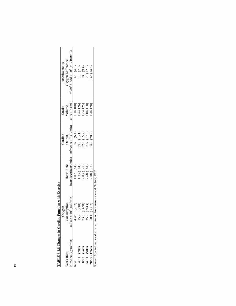
97 TAB

LE 3

.2.8

Cha

nges

in C

ardi

ac F

unct

ion

with

Exe

rcise

O

xyge

n

C

ardi

ac

Stro

ke

Arte

riove

nous

W

ork

Rat

e,

Con

sum

ptio

n,

Hea

rt R

ate,

O

utpu

t, V

olum

e,

Oxy

gen

Diff

eren

ce,

N·m

/sec

(kg·

m/m

in)

m3 /s

ec x

106 (m

L/m

in)

beat

s/se

c(be

ats/

min

)m

3 /sec

x 1

06 (L/m

in)

m3 x

106 (m

L)

m3 /m

3 blo

od x

103 (m

L/10

0mL)

R

est

4.

45

(267

)1.

07

(64)

107

(6.4

)10

0 (10

0)

43

(4.3

)47

.1

(288

)15

.2

(910

)1.

73 (1

04)

218

(13.

1)12

6 (12

6)

70

(7.0

)88

.2

(540

)23

.8

(143

0)2.

03 (1

22)

253

(15.

2)12

5 (12

5)

94

(9.4

)14

7.1

(900

)35

.7

(214

3)2.

68 (1

61)

297

(17.

8)11

0 (11

0)

123

(12.

3)20

5.9

(126

0)50

.1

(300

7)2.

88 (1

73)

348

(20.

9)12

0 (12

0)

145

(14.

5)So

urce

: Ada

pted

and

use

d w

ith p

erm

issio

n fro

m A

smus

sen

and

Nie

lsen,

195

2.

98

Internal work, or physiological work done by the muscle in developing tension, does not necessarily show up as external work. Isometric31 muscle contraction, for instance, does not result in any external work but does represent a physiological oxygen cost (see Section 5.2.5). The length-tension relationship for cardiac muscle tissue (Figure 3.2.9) shows that muscle tension depends on the amount of stretching to which the muscle is subjected. In the heart, this translates into the amount of blood in the ventricular chambers before systole begins. Thus the amount of internal work of the heart depends partly on the end-diastolic volume of blood in the ventricles. The other determinant of internal work is external work. The higher the level of external work, the higher is internal work. Muscular mechanical efficiency is defined as

usedenergytotal

workmechanicalexternal=η (3.2.50)

where η = mechanical efficiency, dimensionless Mechanical efficiency of the heart is quite low, being 3-15%, and may rise to 10-15% when external work is increased (Michie and Kline, 1976). Thus when external work is doubled, internal work is also nearly doubled. With no external work performed, internal work will be minimal; with high blood pressures to overcome, or with the myocardium in a disadvantageous position on the length-tension relationship, internal work will be very high.32 Studies have shown that (1) stroke volume can be delivered with a minimum myocardial shortening if the contraction begins at a larger volume; (2) internal energy usage is lower for a heart at larger volume; (3) higher blood pressures can be attained by stretched muscle fibers; (4) lower amounts of energy are used for slower contraction times (lower heart rate); and (5) the greater the heart volume, the higher the muscle tension required to sustain a given intraventricular pressure (Astrand and Rodahl, 1970). All but the last factor indicates that a more efficient cardiac output would occur with higher stroke volume and lower heart rate. This has been seen to be the trend for trained athletes. For the cardiac patient, large diastolic filling is sometimes accompanied by small stroke volume and high heart rate. Heart dilatation gives improved ability of the muscle fibers to produce tension as long as they are stretched (Astrand and Rodahl, 1970). However, the high heart rate and the high muscle tension combine to use more oxygen than the capillaries of the heart can deliver during mild exercise.33 The result is myocardial hypoxia with symptoms of angina pectoris. It has been reported that left ventricular oxygen consumption is correlated with the product of mean ventricular ejection pressure and the duration of ejection (Michie and Kline, 1976). This is called the tension-time index. Factors that constitute oxygen consumption (proportional to physiological work) of the heart during each beat are (1) resting oxygen consumption, (2) activation oxygen consumption, (3) contraction oxygen consumption, and (4) relaxation oxygen consumption (Michie and Kline, 1976). Resting oxygen consumption is used to maintain the muscle in its healthy, normal relaxed state. Activation oxygen consumption is that used by the muscle as the muscle is excited by a depolarization and repolarization wave (see Sections 1.3.1 and 2.2.2). Contraction oxygen consumption includes internal and external work associated with the development of muscle tension. Relaxation energy is a small (approximately 9%) amount of energy required for the muscle to return to its relaxed state (Michie and Kline, 1976). Power output by the heart, assuming in Equation 3.2.48 a left ventricular systolic pressure of 16 kN/m2, a stroke volume of 70 x 10-6 m3 , a heart rate of 1.2 beats/sec, a right ventricular 31Muscle tension produced at constant length. 32The term preload is often used to describe the effect of initial fiber length, determined by intraventricular pressure and volume. Afterload is the term used to account for the external pressure developed by the ventricle. It is determined by intraventricular pressure and wall thickness, vascular resistance and pressure, and force-velocity relationship of the myocardium (Michie and Kline, 1976). 33While the cardiac muscle is contracting, capillaries in the muscle are being squeezed, allowing less blood to flow.

99

systolic pressure of one-sixth of the left ventricle, and a 10% increase to account for kinetic power, is about 1.8 N·m/sec (Michie and Kline, 1976). During exercise, when maximum systolic pressure may exceed 26.7 kN/m2 and heart rate may be 2.5 beats/sec, kinetic power accounts for about 20% of the total cardiac power of about 8.4 N·m/sec (Michie and Kline, 1976). It has been suggested (Hämäläinen, 1975) that blood flow and pressure can be predicted based on an optimization process. This seems to indicate that, like respiration (see Section 4.3.4), cardiodynamics are driven by a control system that tends to limit the amount of work expended during each cycle. Hämäläinen suggested a cost functional of

( )dtVppJet

02

∫ += �α (3.2.51)

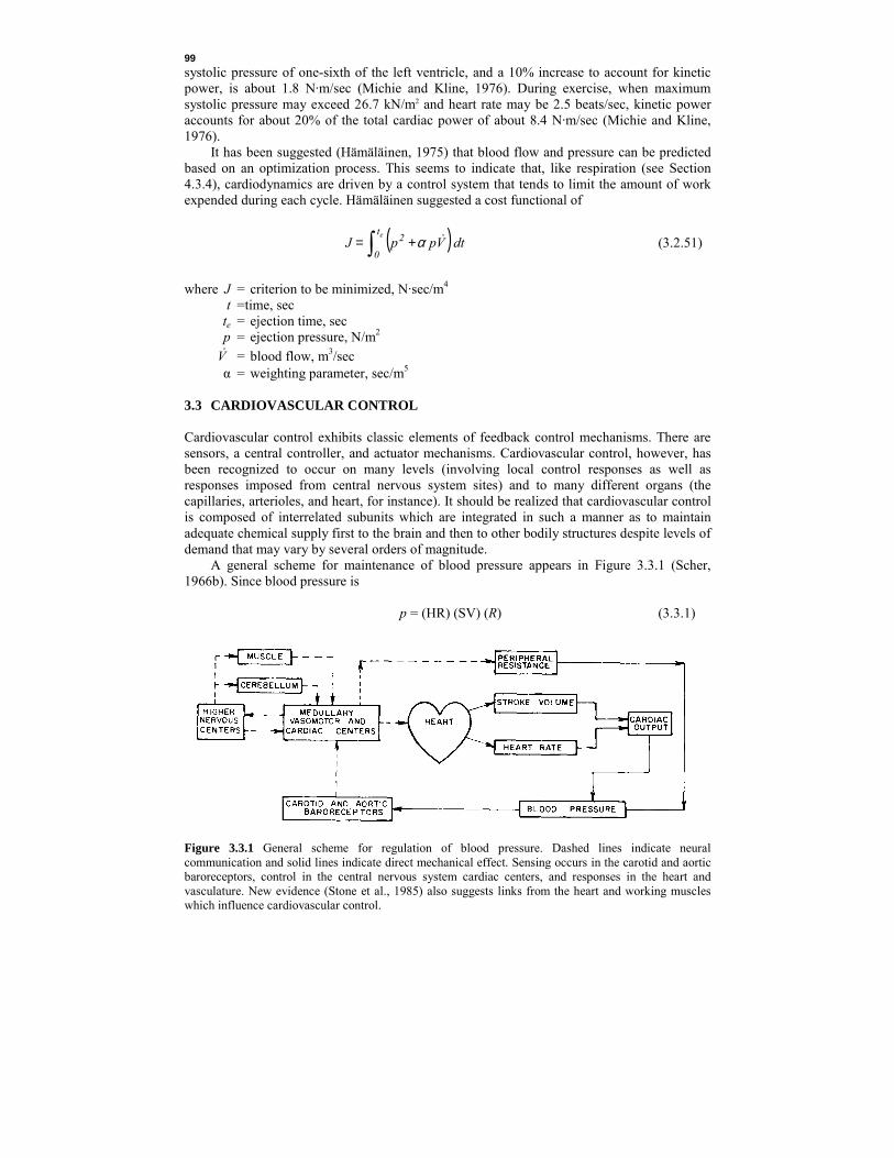
where J = criterion to be minimized, N·sec/m4 t =time, sec te = ejection time, sec p = ejection pressure, N/m2 V� = blood flow, m3/sec α = weighting parameter, sec/m5 3.3 CARDIOVASCULAR CONTROL Cardiovascular control exhibits classic elements of feedback control mechanisms. There are sensors, a central controller, and actuator mechanisms. Cardiovascular control, however, has been recognized to occur on many levels (involving local control responses as well as responses imposed from central nervous system sites) and to many different organs (the capillaries, arterioles, and heart, for instance). It should be realized that cardiovascular control is composed of interrelated subunits which are integrated in such a manner as to maintain adequate chemical supply first to the brain and then to other bodily structures despite levels of demand that may vary by several orders of magnitude. A general scheme for maintenance of blood pressure appears in Figure 3.3.1 (Scher, 1966b). Since blood pressure is

p = (HR) (SV) (R) (3.3.1)

Figure 3.3.1 General scheme for regulation of blood pressure. Dashed lines indicate neural communication and solid lines indicate direct mechanical effect. Sensing occurs in the carotid and aortic baroreceptors, control in the central nervous system cardiac centers, and responses in the heart and vasculature. New evidence (Stone et al., 1985) also suggests links from the heart and working muscles which influence cardiovascular control.

100

TABLE 3.3.1 Cardiovascular Values at Rest and Exercise Work Rate, N·m/sec

Mean Blood Pressure,

kN/m2 x 103

Heart Rate, beats/sec

Stroke Volume, m3 x 106

Cardiac Output,

m3/sec x 106

Peripheral Resistance,

N·sec/m5 x 10-6

Rest 200

13.3 18.9

1.1 2.9

100 120

107 348

121 54

where p = blood pressure, N·m2

HR = heart rate, beats/sec SV = stroke volume, m3

R = peripheral vascular resistance, N·sec/m5

blood pressure can be maintained by changing heart rate, stroke volume, or peripheral vascular resistance. Table 3.3.1 includes typical values for these variables and shows that heart rate during exercise usually increases greatly and vascular resistance greatly decreases. Stroke volume does not change much. To decrease vascular resistance, most blood vessels must open wider. However, the storage vessels must close, because otherwise sufficient amounts of blood would not quickly return to the heart. This is just one illustration of the sometimes contradictory demands placed on the cardiovascular system to reestablish stable equilibrium. 3.3.1 Neural Regulation These responses are coordinated through the central nervous system by means of cardiovascular sensors, a central controller, and various responsive organs. Sensors. There are several different types of sensors which provide input for cardiovascular control. There is first a general class of mechanoreceptors comprised of stretch receptors and baroreceptors. Stretch receptors exist in the carotid sinus and aortic arch, baroreceptors are located in both branches of the pulmonary artery, and volume receptors are in the left and right atria. These receptors, especially in the carotid sinus and aortic arch, generally function in the maintenance of adequate arterial pressure. The firing rate of these sensors reflects mean pressure as well as rates of changes in pressure. For the carotid sinus stretch receptors, the rate of impulses has been expressed (Attinger, 1976b) as

[ ]thth )( pppptdpd

tdpd

tdpd

tdpdf 0 −−+

−+

= −+ δβδβδβ (3.3.2)

where f = neural firing rate, impulses/sec p = arterial pressure, N/m2 t = time, sec pth = threshold arterial pressure, N/m2 δ[x] = 1, x ≥ 0 = 0, x < 0 β+, β– = sensitivity coefficients, m2/N β0 = sensitivity coefficient, m2/(N·sec) The magnitudes of threshold pressure and sensitivity coefficients vary with level of mean pressure. The relationship between the mean sinus pressure and average carotid sinus baroreceptor neural firing rate is sigmoid (Figure 3.3.2) with normal blood pressure in the midportion of the curve (Ganong, 1963) where the sensitivity (rate of change of firing rate to rate of change of mean arterial pressure) is greatest. Pulsating pressures result in greater firing rates.

101

Figure 3.3.2 Average firing rate of a single carotid baroreceptor unit responding to arterial pressure. There is both an influence of pressure and rate of change of pressure on firing rate. (Adapted and used with permission from Korner, 1971.) There are also arterial peripheral chemoreceptors in the aortic arch and carotid sinus sensitive to arterial pO2, pCO2, and pH (Attinger, 1976b). Although they are more important in the regulation of respiration, they do influence cardiovascular responses in extreme circumstances. There appears to be a very small cardiovascular influence, as well, from other peripheral sensors. Lung inflation receptors represent the largest group of vagal afferent sources (Attinger, 1976b) and, since the heart is also innervated by the vagus, may play a role in the interaction seen between respiration and cardiac output. Somatic inputs through the trigeminal nerve are important in relation to the diving and nasal circulatory reflexes.34

Controller. The heart is capable of generation of its basic rhythm in the absence of external neural inputs and can maintain some local regulation of its output. However, the cardiovascular controller must integrate numerous pieces of afferent information into a coherent strategy for effective cardiovascular response. Much of this integration occurs in the reticular substance of the lower pons and upper medulla (Figure 3.3.3) and is called the vasomotor center. Its lateral portions are continuously sending efferent signals to partially contract the blood vessels (vasomotor tone). The medial part of the center transmits inhibitory signals to the lateral part, which results in vasodilation (Attinger, 1976b). The lateral vasomotor center also transmits impulses through sympathetic nerve fibers to the heart, which results in cardiac acceleration and increased contractility (Attinger, 1976b). The inhibitory center, on the other hand, is connected to the heart via the parasympathetic35 fibers of the vagus nerve and tends to slow heart rate and relax the myocardium (Figure 3.3.4). The entire cardiovascular regulatory system is not localized in one section of the central nervous system (Smith, 1966). The vasomotor center is normally influenced by peripheral baroreceptor and chemoreceptor inputs, central nervous system chemoreceptor inputs, the 34The diving reflex is an apparently primordial action which results in a significant lower heart rate when the face is suddenly chilled. 35The sympathetic nervous system is involved in reactions to stress; these include increasing heart rate, respiration rate, sweating, and secretion of adrenaline. The parasympathetic system is normally antagonistic to the sympathetic system and is used to maintain resting homeostasis: slow heart rate, maintaining gastrointestinal activity, and promoting balanced endocrine secretions. The sympathetic system acts on beta adrenergic receptors of the heart, whereas the parasympathetic system acts on gamma receptors.

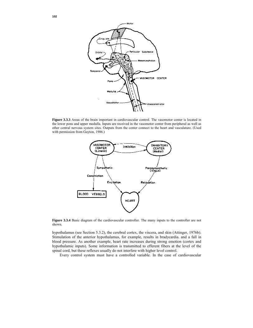
102

Figure 3.3.3 Areas of the brain important in cardiovascular control. The vasomotor center is located in the lower pons and upper medulla. Inputs are received in the vasomotor center from peripheral as well as other central nervous system sites. Outputs from the center connect to the heart and vasculature. (Used with permission from Guyton, 1986.)

Figure 3.3.4 Basic diagram of the cardiovascular controller. The many inputs to the controller are not shown. hypothalamus (see Section 5.3.2), the cerebral cortex, the viscera, and skin (Attinger, 1976b). Stimulation of the anterior hypothalamus, for example, results in bradycardia. and a fall in blood pressure. As another example, heart rate increases during strong emotion (cortex and hypothalamic inputs). Some information is transmitted to efferent fibers at the level of the spinal cord, but these reflexes usually do not interfere with higher level control. Every control system must have a controlled variable. In the case of cardiovascular

103

TA

BL

E 3

.3.2

Blo

od F

low

and

Oxy

gen

Con

sum

ptio

n of

Var

ious

Org

ans i

n a

617

N (6

3 kg

) Adu

lt H

uman

with

a M

ean

Art

eria

l Blo

od P

ress

ure

of 1

2 kN

/m2

(90

mm

Hg)

and

an

Oxy

gen

Con

sum

ptio

n of

4.1

7 x

10-6 m

3 /sec

(250

mL

/min

) Pe

rcen

tage

of T

otal

Reg

ion

M

ass,

kg

B

lood

Flo

w,

m3 /s

ec x

106 (m

L/m

in)

A

rterio

veno

us

Oxy

gen

Diff

eren

ce,

m3 /m

3 blo

od x

103 (m

L/L)

Oxy

gen

Con

sum

ptio

n,

m3 /s

ec x

106 (m

L/m

in)

Vas

cula

r R

esis

tanc

e,a

N·se

c/m

5 x 1

0-6

(mm

Hg·

sec/

mL)

C

ardi

ac

Out

put

Oxy

gen

Con

sum

ptio

nLi

ver

Kid

neys

B

rain

Sk

in

Skel

etal

mus

cle

Hea

rt m

uscl

e R

est o

f bod

y To

tal

2.6

0.3

1.4

3.6

31.0 0.3

23.8

63.0

25.0

21

.0

12.5

7.

7 14

.0

4.2

5.6

90.0

(150

0)(1

260)

(750

)(4

62)

(840

)(2

50)

(336

)(5

400)

34

14

62

25

60

11

4 12

9 46

(34)

(14)

(62)

(25)

(60)

(114

)(1

29)

(46)

0.

85

0.30

0.

77

0.20

0.

83

0.48

0.

73

4.17

(51)

(18)

(46)

(12)

(50)

(29)

(44)

(250

) 48

0 57

1 96

0 15

60

857

2880

21

40

133

(3.6

)(4

.3)

(7.2

)(1

1.7)

(6.4

)(2

1.4)

(16.

1)(1

.0)

27.8

23.3

13.9 8.6

15.6 4.7

6.2

100.

0 20

.4 7.2

18.4 4.8

20.0

11.6

17.6

100.

0So

urce

: Ada

pted

and

use

d w

ith p

erm

issi

on fr

om B

ard,

196

1.

a Vas

cula

r res

ista

nce

is m

ean

arte

rial b

lood

pre

ssur

e (1

2 kN

/m2 ) d

ivid

ed b

y bl

ood

flow

.

104

control, as in the cases of most other controlled systems discussed in this book, maintenance of a normal operating environment for the brain appears to be the controlled variable. The cerebral vessels possess very little vasodilatory innervation, which is of little functional importance. Instead, regulatory mechanisms maintain total cerebral blood flow under widely varying conditions.36 Total cerebral blood flow is not increased by strenuous mental activity, and it does not decrease during sleep. One reason for this may be that oxygen consumption of the human brain is very high, averaging 5.8 x 10-8 m3/sec (3.5mL/min) per gram brain tissue, or 82 x 10-8 m3/sec (49mL/min) for the whole brain in an adult (Ganong, 1963). This figure represents approximately 20% of the total resting oxygen consumption (Table 3.3.2). Brain tissue is extremely sensitive to anoxia, and unconsciousness occurs about 10 seconds after the blood supply is interrupted. When blood flow to the brain is decreased, cardiovascular control mechanisms quickly attempt to return it to normal. For instance, if intracranial pressure is somehow elevated to more than 4400 N·m2 (33 mm Hg), cerebral blood flow is soon significantly reduced (Ganong, 1963). The resultant ischemia stimulates the vasomotor center and systemic blood pressure rises. As intracranial pressure is made to increase further, systemic blood pressure rises proportionately. Similarly, local changes in CO2 and O2 partial pressures in the blood can change cerebral blood flow. A rise in pCO2 exerts a profound vasodilator effect on the arterioles. A low pO2 will likewise cause vasodilation. Low pCO2 or high pO2 results in mild vasoconstriction.37 These effects result in a certain degree of autoregulation of blood flow to maintain the chemical milieu of the brain within tolerable limits. It therefore appears likely that the most sensitively regulated area is the brain, and that most cardiovascular regulatory responses are those associated with maintaining homeostasis of the brain. Effector Organs. All blood vessels with the exception of capillaries and venules are innervated by sympathetic autonomic nerve fibers. The arterioles and other resistance vessels are the most densely innervated. Resistance of these vessels is regulated to control tissue blood flow and arterial pressure. The veins, which act as capacitance, or storage, vessels (Table 3.2.2), are regulated to control the amount of stored blood. Venoconstriction and arteroconstriction occur together, shifting blood to the arterial side of the circulation. In addition, vasoconstriction in the gastrointestinal area decreases blood flow to the gastrointestinal system, liver, and spleen. Other important blood reservoirs at rest are the skin and lungs. During severe exercise, constriction of the vessels in these organs, as well as decreased blood volume in the liver and splanchnic bed, may increase actively circulating blood volume perfusing the muscles by as much as 30% (Table 3.2.3). Thus vascular innervation causes two types of physical control response: (1) peripheral resistance changes to maintain blood pressure regulation and (2) blood distribution changes to maintain blood flow to tissues which require delivery of metabolites and oxygen. Beneken and DeWit (1967) discussed with unusual clarity the role of peripheral resistance control in local and systemic regulation. Central nervous system regulation of peripheral arterial resistance occurs when arterial pressure changes and is due to baroreceptor sensing of central blood pressure. Vasoconstriction occurs when arterial pressure falls; therefore, central nervous system control can be thought of as a pressure-controlling system. Autoregulation, the local response to inadequate tissue nutrition, allows local vascular beds to open to increase blood flow. Autoregulation mainly serves to ensure an adequate distribution of cardiac output to the various parts of the body and is so local that it has almost no direct effect on heart action and total cardiac output. Central nervous system control of arterial blood flow can be overridden by autoregulation when local tissue oxygen consumption exceeds blood oxygen delivery. Thus autoregulation can be thought of as a flow-controlling system. 36Cerebral blood flow in adults averages 9 x 10-6 m3/sec (0.54L/min) per kilogram brain tissue with a normal range of 6.7-11.2 x 106 m3/(sec·kg) (0.40-0.67 L/kg min) (Ganong, 1963). 37The unconsciousness that results from severe hyperventilation is the result of arteriolar hypocaphic vasoconstriction, reducing the blood flow to parts of the brain.

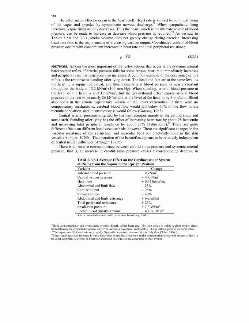
105

The other major effector organ is the heart itself. Heart rate is slowed by continual firing of the vagus and speeded by sympathetic nervous discharge.38 When sympathetic firing increases, vagus firing usually decreases. Thus the heart, which is the ultimate source of blood pressure, can be made to increase or decrease blood pressure as required.39 As we saw in Tables 3.2.8 and 3.3.1, stroke volume does not greatly change during exercise. Increasing heart rate thus is the major means of increasing cardiac output. Coordinated control of blood pressure occurs with concomitant increases in heart rate and total peripheral resistance:

RVp C= (3.3.3) Reflexes. Among the most important of the reflex actions that occur is the systemic arterial baroreceptor reflex. If arterial pressure falls for some reason, heart rate immediately increases and peripheral vascular resistance also increases. A common example of the occurrence of this reflex is the response to standing after lying down. The head and feet are at the same level as the heart in a supine individual, and thus mean arterial blood pressure is nearly constant throughout the body at 13.3 kN/m2 (100 mm Hg). When standing, arterial blood pressure at the level of the heart is still 13 kN/m2, but the gravitational effect causes arterial blood pressure in the feet to be nearly 26 kN/m2 and at the level of the head to be 8-9 kN/m2. Blood also pools in the venous capacitance vessels of the lower extremities. If there were no compensatory mechanisms, cerebral blood flow would fall below 60% of the flow in the recumbent position, and unconsciousness would follow (Ganong, 1963). Central arterial pressure is sensed by the baroreceptors mainly in the carotid sinus and aortic arch. Standing after lying has the effect of increasing heart rate by about 25 beats/min and increasing total peripheral resistance by about 25% (Table 3.3.3).40 There are quite different effects on different local vascular beds, however. There are significant changes in the vascular resistance of the splanchnic and muscular beds but practically none in the skin vessels (Attinger, 1976b). The operation of the baroreflex appears to be relatively independent of central neural influences (Attinger, 1976b). There is an inverse correspondence between carotid sinus pressure and systemic arterial pressure; that is, an increase in carotid sinus pressure causes a corresponding decrease in

TABLE 3.3.3 Average Effect on the Cardiovascular System of Rising from the Supine to the Upright Position Variable Change Arterial blood pressure Central venous pressure Heart rate Abdominal and limb flow Cardiac output Stroke volume Abdominal and limb resistance Total peripheral resistance Small vein pressure Pooled blood (mostly venous)

0 kN/m2

– 400 N/m2

+ 0.42 beats/sec – 25% – 25% – 40% + (variable) + 25% + 1.3 kN/m2

– 400 x 10-6 m3 Source: Adapted and used with permission from Greg, 1961.

38Both parasympathetic and sympathetic systems directly affect heart rate. This rate action is called a chronotropic effect. Stimulation by the sympathetic system, moreover, increases myocardial contractility. This is called a positive inotropic effect. 39The vagus can affect heart rate very rapidly. Sympathetic control, however, is relatively slow (Scher, 1966b). 40Since vagal heart rate response is much faster than sympathetic response, initial compensation to postural change is likely to be vagal. Sympathetic effects on heart rate and blood vessel resistance occur later (Scher, 1966b).

106

Figure 3.3.5 Relationship between mean carotid sinus pressure and mean systemic arterial pressure. The similarity between these two pressures and the neural output from the carotid sinus (Figure 3.3.2) should be noted. (Adapted and used with permission from Korner, 1971.) arterial pressure. There is a strong similarity between the carotid sinus firing rate curve (Figure 3.3.2) and the systemic pressure response curve (Figure 3.3.5) when the systemic pressure response curve is inverted. Incremental gain of the system, usually defined as change in output divided by change of input, varies with pressure. It is a maximum where the slope of the systemic pressure response curve is a maximum.41 In Figure 3.3.5, this occurs at nearly normal carotid sinus pressure of 16.7 kN/m2 [data for dog (Scher, 1966b)]. Since incremental gain is not constant, it is not surprising that the arterial pressure response for a pulsatile pressure is not the same as for a constant pressure. Since incremental gain decreases away from a pressure corresponding to gain maximum, arterial pressure response is lower for a pressure pulsating between maximum gain pressure and some lower pressure. Since pressures are sensed at two main locations (carotid sinus and aortic arch), it is of interest to know that somewhat the same systemic arterial response can be obtained from increased pressure on any one location. That is, the magnitude of the overall effect does not correspond to the algebraic sum of the individual effects (Attinger, 1976b) but instead appears to be a case of biological redundancy. The open-loop gain of the aortic arch appears to be one-quarter to one-half that of the carotid sinus receptors (Burton, 1965). Scher (1966b) has given an analysis of the systemic arterial baroreceptor reflex. An approximation to the variable gain in Figure 3.3.5 is

−+

∆∆

−=∆∆ n

ssss

pppp

pp

)(max| max1βαα (3.3.4)

where ∆pα = change in output (arterial) pressure, N/m2 ∆ps = change in input (carotid sinus) pressure, N/m2 ps = carotid sinus pressures, N/m2 ps max = carotid sinus pressure corresponding to the maximum gain, (∆pα/∆ps)|max, N/m2 β1 = coefficient, (m2/N)n n = an even number, dimensionless 41Scher (1966b) reports a maximal gain of 10- 15 in some cats.

107

To account for the effects of pulsatile pressure, where a varying carotid sinus pressure decreases the resulting arterial pressure despite maintenance of a constant mean pressure, a recitification equation has been proposed. Also included in this equation is the observation that as the frequency or amplitude of these changes increases, arterial pressure falls further (Scher, 1966b).

αp∆ = –G(ps + dps/dt – β2) [Sgn(ps + dps/dt – β2)] (3.3.5)

where αp∆ = change in mean output pressure due to pulsating carotid sinus pressure, N/m2 t = time, sec β2 = constant, N/m2 G = amplification, factor, dimensionless Sgn(x) = +1, x > 0 = –1, x < 0 Finally, to describe the pressure response to transient changes, notably square- and sine-wave inputs, Scher (1966b) presents a linear approximation. Response to an input pressure square wave is composed of a 2-4.5 sec period before any response, followed by an early overshoot and then a slow (up to 100 sec) decline to the new level.

[ ])(2

2

43 ds tt

dtdp

tdpd

tdpd

−=+ δββ αα (3.3.6)

where β3 = coefficient, dimensionless β4 = coefficient, sec·m2/N td = time delay δ(t – td) = 1, t > td = 0, td < t There are other cardiovascular reflexes with neural origin. A pulmonary artery baroreceptor reflex primarily controls respiration by reducing ventilation by approximately 20% for each 130 N/m2 rise in pulmonary arterial pressure; cardiovascular effects become significant when arterial pressure change exceeds 8 kN/m2 (Attinger, 1976b). Cardiac mechanoreceptor reflexes are similar to, but much weaker than, the carotid sinus reflex; when strongly stimulated, epicardial and ventricular receptors produce bradycardia, hypotension, and reduced respiration (Attinger, 1976b). The arterial chemoreceptor reflex most strongly affects respiration, but it does have cardiovascular consequences; hypoxia and hypercapnia result in bradycardia, total peripheral resistance increase, arterial blood pressure increase, and catecholamine secretion increase. Heart rate is accelerated, and consequent blood pressure is increased, by decreased baroreceptor activity, respiratory inspiration, excitement, anger, painful stimuli, anoxia, exercise, and humoral agents (Faucheux et al., 1983; Lindqvist et al., 1983). Heart rate is slowed by increased baroreceptor activity, expiration,42 fear, grief, the diving reflex, and increased intracranial. pressure (Ganong, 1963). Tranel et al. (1982) demonstrated that monetary rewards were sufficient to cause significant changes in heart rate when they were given to test subjects for desired heart rate modifications. 3.3.2 Humoral Regulation Not all cardiovascular regulation is neural. Circulating hormones, metabolites, and regulators also have cardiovascular effects. These are effective mostly at the local level. For instance, 42Mehlsen et al. (1987) report that suddenly initiated (stepwise) inspiration and expiration both resulted in an increase in heart rate followed by a rapid decrease in heart rate. Heart rate was thus seen to respond to changes in lung volume. Coherent changes in heart rate and breathing are commonly referred to as respiratory sinus arrhythmia (Kenney, 1985).

108

chemical substances that directly act on arteriole muscle fibers to cause local vasodilation are decreased oxygen partial pressure, decreased blood and tissue pH, increased carbon dioxide pressure (especially vasodilates the skin and brain), lactic acid, and adenylic acid (Ganong, 1963).43 Histamine released from damaged cells dilates capillaries and increases their permea-bility (Ganong, 1963). Bradykinin secreted by sweat glands, salivary glands, and the exocrine portion of the pancreas vasodilates these secreting tissues (Ganong, 1963). Other substances cause vasoconstriction. Injured arteries and arterioles constrict from serotonin liberated from platelets sticking to vessel walls (Ganong, 1963). Norepinephrine has a general vasoconstrictor action. Diurnal variations of norepinephrine have been found to be associated with a mean arterial blood pressure 3700 N/m2 (28 mm Hg) lower during the middle of the night than during the day (Richards et al., 1986). Epinephrine is also a general vasoconstrictor in all but the liver and skeletal muscle, which it vasodilates. The net effect of epinephrine is thus a decrease in total peripheral resistance (Ganong, 1963). Norepinephrine and epinephrine both increase the force and rate of contraction of the isolated heart (Ganong, 1963). Norepinephrine increases systolic and diastolic blood pressure, which, in turn, stimulates the aortic and carotid sinus barorecptors to produce bradycardia, leading to decreased cardiac output. Norepinephrine, epinephrine, and thyroxin all increase heart rate (Ganong, 1963). It is likely that prostaglandins will also be found to have cardiovascular regulatory roles. 3.3.3 Other Regulatory Effects Other effects are locally important in cardiovascular regulation. We have already noted Starling's law (Section 3.2.3), which increases the contractility of myocardium in response to preload. This is important for equalization of cardiac output between the left and right hearts. Temperature is also an important cardiovascular regulator. High environmental temperature or fever increases heart rate. A rise in temperature in muscle tissue directly causes arteriole vasodilation (Ganong, 1963). Total blood volume is controlled indirectly through capillary pressure (see Section 3.2.2). When capillary pressure increases, fluid leaks into the cellular interstitium. When capillary pressure falls below its normal value of about 3300 N/m2, fluid is absorbed into the circulatory system. Capillary pressure is controlled indirectly by the same artery and venous innervation that controls blood pressure. Renal output also can be used to control total blood volume.44 Hemorrhage usually results in a large reduction of urinary output, and fluid infusion stimulates urinary production. These adjustments are long term, however, and require a day or more to complete; capillary fluid shift requires only a few hours (Beneken and DeWit, 1967). This mix of neural, humoral, and other local mechanisms allows cardiovascular adjustments to be very efficient. The redundancy of effects underscores the importance of the cardiovascular system. 3.3.4 Exercise All previously presented effects are manifested during exercise (Hammond and Froelicher, 1985). Exercise increases carbon dioxide production by the muscles, which, in turn, increases venous pCO2, and this stimulates cardiovascular responses. Heart rate increases, stroke 43Adenylic acid is another term for adenosine monophosphate, or AMP, the energy-poor precursor of adenosine triphosphate, or ATP. 44Reeve and Kulhanek (1967) outlined an interesting, if rudimentary, model of body water content regulation. This mathematical model includes elements of urinary water excretion and drinking set in a context of a water balance for the entire body.

109

volume remains nearly the same, and cardiac output increases (Figure 3.3.6). The increase in heart rate is nearly linear with work rate (Equation 3.2.42),45 except near maximum oxygen uptake where gains in oxygen uptake depend not only on the amount of blood delivered to the tissues (as indicated by heart rate) but also on the oxygen-carrying capacity of the blood (as indicated by pO2). Venous pO2 falls near maximum oxygen uptake, meaning that the muscles are increasing oxygen use without a concomitant increase in heart rate.

Blood volume is moved from the venous side of the heart to the arterial side during exercise. Stroke volume may actually fall during maximal exercise because venous return is insufficient to completely fill the atrium during each heartbeat. Venous return is enhanced by muscle pumping. Cardiac output, composed of stroke volume and heart rate, increases to a maximum value at maximal oxygen uptake. If no differences in arterial-to-venous pO2 occur, oxygen uptake is directly related to cardiac output. The increase in heart rate occurring at the beginning of exercise is very rapid (Figure 3.3.7). Sometimes the increase even precedes the start of exercise, which indicates that neural control from higher nervous centers (through the sympathetic nervous system), rather than arterial pO2 or pCO2 changes, are at least temporarily dominant (see Jones and Johnson, 1980; Mitchell, 1985; Perski et al., 1985). The increase of heart rate is higher for a given oxygen uptake for arm exercise compared to leg exercise. Moving the arms above the head increases heart rate more than moving the arms below the neck. Static (isometric) exercise increases heart rate disproportionately to that expected from oxygen uptake alone. Increased muscle temperature, increased carbon dioxide concentration, decreased pH, and decreased oxygen concentration all have local vasodilatory effects. Blood flow through working muscle is thus increased. Central nervous system control of vessel caliber is added to local effects, thus shifting blood flow from regions with lower oxygen demand (especially the viscera) to regions with higher demand. Total peripheral resistance decreases. Because of this, diastolic pressures may actually decrease (although they may increase) somewhat despite higher blood flows (Comess and Fenster, 1981). Systolic pressures increase and mean blood pressure increases during exercise. Females generally tend to exhibit higher heart rates than males at comparable percentages of maximal oxygen uptake. Trained athletes have no higher maximum heart rates than untrained individuals.46 However, they usually develop larger hearts capable of delivering larger stroke volumes. For any rate of oxygen uptake, athletes' hearts are able to deliver the required output with lower heart rates than can untrained individuals. The cardiac hypertrophy developed in trained individuals is difficult to distinguish from similar conditions developed by individuals with impaired cardiac function (Schaible and Scheuer, 1985). The athletic heart, however, exhibits enhanced performance,47 whereas pathologic cardiac hypertrophy is an adjustment made by parts of the heart to overcome shortcomings of other parts of the cardiovascular system. Chemical changes that occur improve oxygen transport to the muscles (including the myocardium). The hemoglobin dissociation curve (Figures 3.2.1 through 3.2.3) shifts with increased pCO2, decreased pH, and increased temperature to deliver oxygen with greater ease to the working muscles. That is, for any given percentage saturation, the factors just cited tend to increase plasma pO2 and allow more O2 to move into the interstitial fluid and muscle cells. Muscle oxygen consumption, by these mechanisms, can increase above resting values by 75-100 times. Even higher increases are possible for very limited amounts of time by utilizing anaerobic metabolism. 45Except for an additional increment of heart rate increase with increased deep body temperature (see Section 3.4.5). 46Erikssen and Rodahl (1979) showed that seasonal variations in physical fitness can exist in a population. Because of this, comparisons of results between exercise tests conducted at different times of the year may be invalid. 47This cardiac condition is even marked by electrocardiographic (ECG) signals that resemble those from severely ill patients.

110

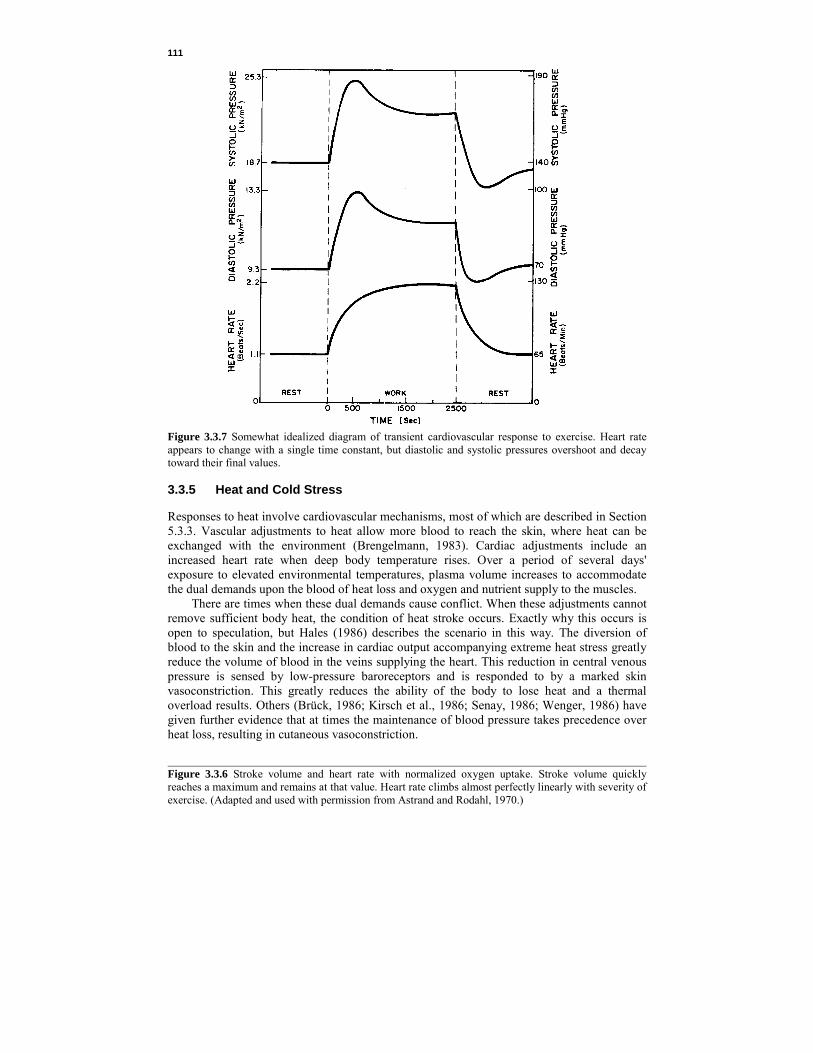
111

Figure 3.3.7 Somewhat idealized diagram of transient cardiovascular response to exercise. Heart rate appears to change with a single time constant, but diastolic and systolic pressures overshoot and decay toward their final values. 3.3.5 Heat and Cold Stress Responses to heat involve cardiovascular mechanisms, most of which are described in Section 5.3.3. Vascular adjustments to heat allow more blood to reach the skin, where heat can be exchanged with the environment (Brengelmann, 1983). Cardiac adjustments include an increased heart rate when deep body temperature rises. Over a period of several days' exposure to elevated environmental temperatures, plasma volume increases to accommodate the dual demands upon the blood of heat loss and oxygen and nutrient supply to the muscles. There are times when these dual demands cause conflict. When these adjustments cannot remove sufficient body heat, the condition of heat stroke occurs. Exactly why this occurs is open to speculation, but Hales (1986) describes the scenario in this way. The diversion of blood to the skin and the increase in cardiac output accompanying extreme heat stress greatly reduce the volume of blood in the veins supplying the heart. This reduction in central venous pressure is sensed by low-pressure baroreceptors and is responded to by a marked skin vasoconstriction. This greatly reduces the ability of the body to lose heat and a thermal overload results. Others (Brück, 1986; Kirsch et al., 1986; Senay, 1986; Wenger, 1986) have given further evidence that at times the maintenance of blood pressure takes precedence over heat loss, resulting in cutaneous vasoconstriction. Figure 3.3.6 Stroke volume and heart rate with normalized oxygen uptake. Stroke volume quickly reaches a maximum and remains at that value. Heart rate climbs almost perfectly linearly with severity of exercise. (Adapted and used with permission from Astrand and Rodahl, 1970.)

112

Cardiovascular responses to cold environments are characterized by cutaneous vasoconstriction to maintain body heat. Wagner and Horvath (1985) reported that men exposed to cold air reacted with increased stroke volume and decreased heart rate. Women exposed to the same environments showed no such change [although Stevens et al. (1987) reported heart rate decreases in men but a slight increase in women, both exposed to cold stress]. Total peripheral resistance of older subjects exposed to cold environments increased more than did that of younger subjects (Wagner and Horvath, 1985). The increase in resistance was so great, in fact, that the resulting increase in mean arterial pressure could cause difficulties for hypertensive48 or angina-prone49 individuals exposed to the cold. They also reported a 10% increase in cardiac output to service increased oxygen demands of shivering. 3.4 CARDIOVASCULAR MECHANICAL MODELS Cardiovascular mechanical models are intended to conceptualize the mechanics of the cardiovascular system. For physiologists, these models are more likely to be in pictorial or graphic form; for bioengineers, these models are more likely to be mathematical in nature. All models of biological systems must include the essentials of the processes described, but these models must be simplifications of reality. Because the cardiovascular system is complicated and includes much of the physical body, cardiovascular models have generally been limited to descriptions of one or two aspects of the system. We have already seen at least one model of this type in the discussion of the Fahraeus-Lindqvist effect in very small blood vessels (Section 3.2.2). Attempts have been made to incorporate cardiodynamics into models of the vascular tree to predict parameters which can be compared to experimental observations. These attempts have included lumped-parameter mechanical models and distributed-parameter mechanical models.50 Use of limited models for prediction of exercise results is not very productive because of the all-inclusive nature of exercise response. We deal with some of these limited models only because it is possible that they might become elements in more comprehensive cardiovascular models. Several general cardiovascular mechanics models are described. We also briefly discuss optimization models in the heart. Finally, two models of a more unrefined, but perhaps useful nature, dealing with heart rate response to exercise challenge, are discussed. 3.4.1 Robinson's Ventricle Model Heart mechanics, especially those of the left ventricle, have been the object of many models (Perl et al., 1986; Sorek and Sideman, 1986a, b). Robinson's model (1965; Attinger, 1976c; Talbot and Gessner, 1973) was developed to test changes of cardiac output with differences of heart muscle mechanics as given by Starling's law (see Section 3.2.3). As such, it is a lumped-parameter mechanical model of the heart and blood vessels. Robinson began at the level of the 48Hypertension is the term given to conditions marked by high blood pressure. Should blood pressure become too high, it can overcome the strength of the walls of the blood vessels and blood would burst out into surrounding tissue. The thinning, stretching, and bulging of weakened blood vessel walls is called an aneurysm, and when a ruptured aneurysm appears in the brain a stroke may result. 49Angina pectoris is the condition where severe chest pain due to ischemia (lack of oxygen leading to tissue necrosis) in the myocardium is caused by inadequate coronary blood circulation. 50Lumped-parameter models assume the entire model segment can be replaced by a very small number of elements, each usually representing one property of the segment. Any spatial dependence of these properties is neglected. Nonlinearities can be included, but waves and other spatial-temporal effects cannot be predicted. Distributed-parameter models are often similar to a large number of lumped-parameter models of subsegments and, because they can account for spatial dependence of segment properties, can reproduce wave behavior. Modeling the vascular system as one resistance, inertance, and compliance is an example of a lumped-parameter model. A distributed-parameter model would include many resistance, inertance, and compliance elements with many interconnections.

113

Figure 3.4.1 The three-element model of the myocardium. The output of the force source fc depends on the length of the parallel element PE and its rate of shortening. Total muscle length equals the length of PE and the shorter length of the series element SE. The force source is assumed to be active only during systole and to be freely distensible in passive muscle. (Used with Permission from Talbot and Gessner, 1973.) myocardium (Figure 3.4.1) by assuming each muscle fiber to be effectively given by a contractile element in parallel with an elastic element and in series with another elastic element (Mende and Cuervo, 1976; Phillips et al., 1982). The force source51 produces a force magnitude depending on the length of the parallel elastic element and on its rate of shortening. Total muscle fiber length is the length of the parallel element (or force source) plus the length of the series element. When muscle fibers are combined into a ventricle model, force elements are all lumped together and series elastic elements are lumped together. Thus the concept of ventricular contraction consists of a force developed by the force elements forcing blood into the elastic portion with concurrent pressure buildup (Figure 3.4.2). The rate of change of volume (dV/dt) is limited by a resistance element which assumes a higher value (Rs) in systole compared to diastole (Rd). Aortic valve resistance (Rav) to outflow and mitral valve resistance (Rmv) to inflow are included. Series element compliance (Cse) is included in the elastic portion. Robinson developed the following differential equation for intraventricular systolic pressure. Beginning with a pressure balance on the ventricle, intraventricular pressure equals the pressure developed by the muscle from which is subtracted pressure dissipated through viscous resistance (actually negative, since dV/dt is negative during systole) and pressure used to overcome compliance; since V = Cp, C(dp/dt) is equivalent to dV/dt,

tdpdCR

tddVRpp sss se−+= (3.4.1)

where Cse = series element compliance, m5/N p = intraventricular pressure, N/m2

V = total ventricular volume (contractile plus elastic compartments), m3

Rs = internal ventricular viscous resistance during systole, N·sec/m5

ps = isometrically developed muscle pressure during systole, N/m2

51Force, pressure, voltage, and temperature are examples of effort variables. An ideal effort source is characterized by a constant effort no matter what the flow. Hence ideal effort sources have zero internal impedances (impedance equals change in effort divided by change in flow). Fluid flow, electrical current, and heat are examples of flow variables. Ideal flow sources are characterized by constant flow rates no matter what effort must be expended to do so. Hence ideal flow sources have infinite internal impedance.

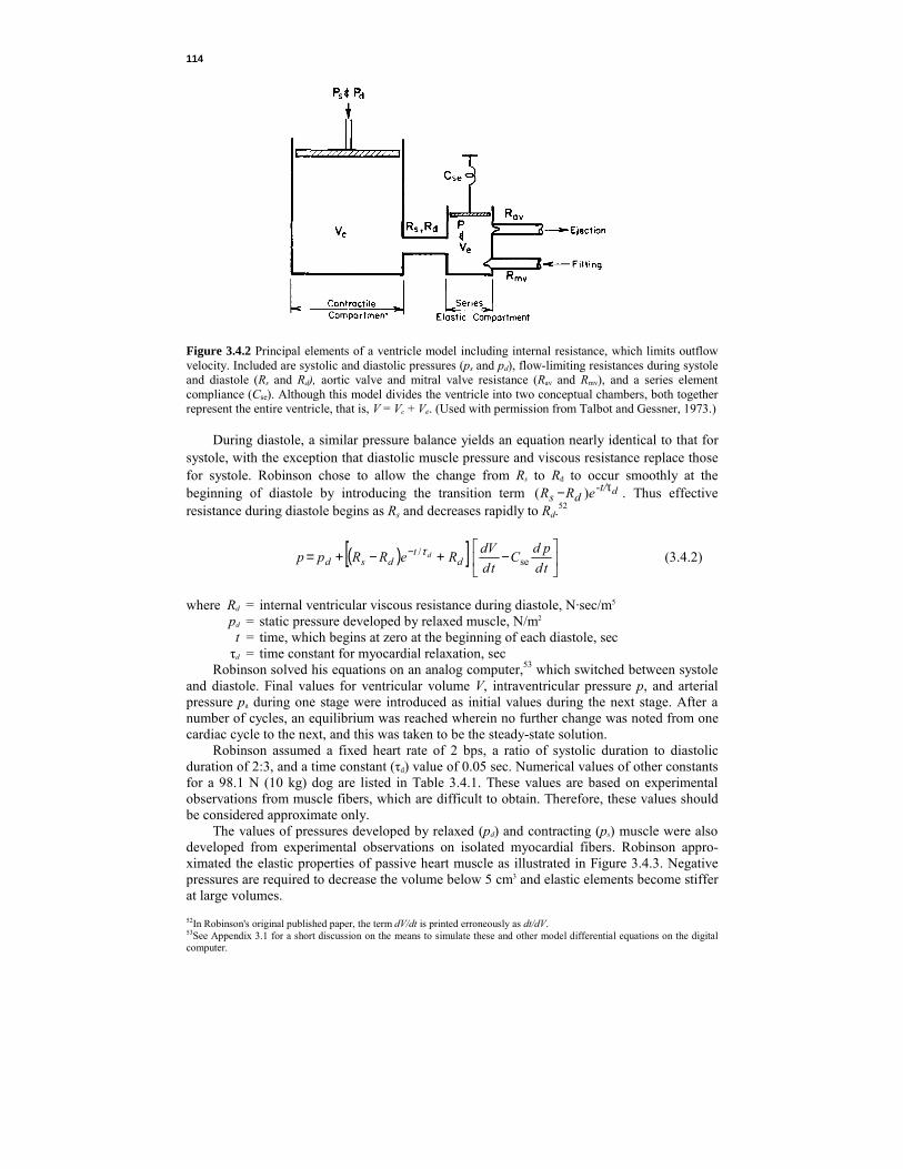
114

Figure 3.4.2 Principal elements of a ventricle model including internal resistance, which limits outflow velocity. Included are systolic and diastolic pressures (ps and pd), flow-limiting resistances during systole and diastole (Rs and Rd), aortic valve and mitral valve resistance (Rav and Rmv), and a series element compliance (Cse). Although this model divides the ventricle into two conceptual chambers, both together represent the entire ventricle, that is, V = Vc + Ve. (Used with permission from Talbot and Gessner, 1973.) During diastole, a similar pressure balance yields an equation nearly identical to that for systole, with the exception that diastolic muscle pressure and viscous resistance replace those for systole. Robinson chose to allow the change from Rs to Rd to occur smoothly at the beginning of diastole by introducing the transition term d-t/

ds eRR τ− )( . Thus effective resistance during diastole begins as Rs and decreases rapidly to Rd.52

( )[ ]

−+−+= −

tdpdC

tddVReRRpp d

tdsd

dse

/τ (3.4.2)

where Rd = internal ventricular viscous resistance during diastole, N·sec/m5 pd = static pressure developed by relaxed muscle, N/m2 t = time, which begins at zero at the beginning of each diastole, sec τd = time constant for myocardial relaxation, sec Robinson solved his equations on an analog computer,53 which switched between systole and diastole. Final values for ventricular volume V, intraventricular pressure p, and arterial pressure pa during one stage were introduced as initial values during the next stage. After a number of cycles, an equilibrium was reached wherein no further change was noted from one cardiac cycle to the next, and this was taken to be the steady-state solution. Robinson assumed a fixed heart rate of 2 bps, a ratio of systolic duration to diastolic duration of 2:3, and a time constant (τd) value of 0.05 sec. Numerical values of other constants for a 98.1 N (10 kg) dog are listed in Table 3.4.1. These values are based on experimental observations from muscle fibers, which are difficult to obtain. Therefore, these values should be considered approximate only. The values of pressures developed by relaxed (pd) and contracting (ps) muscle were also developed from experimental observations on isolated myocardial fibers. Robinson appro-ximated the elastic properties of passive heart muscle as illustrated in Figure 3.4.3. Negative pressures are required to decrease the volume below 5 cm3 and elastic elements become stiffer at large volumes. 52In Robinson's original published paper, the term dV/dt is printed erroneously as dt/dV. 53See Appendix 3.1 for a short discussion on the means to simulate these and other model differential equations on the digital computer.

115

TABLE 3.4.1 Numerical Values for Robinson Model Parameters for a 98 N Dog Parameter Valuea

Heart rate Systole/diastole times Time constant (τd) Resistance of contracting muscle (Rs) Resistance of relaxed muscle (Rd) Total peripheral resistance (Rp) Resistance of aortic valve (Rav) Resistance to filling (Rv) Compliance of ventricle (Cse) Compliance of arterial system (Cp) Filling pressure (Pv)

2 bps 2:3 0.05 sec 333 x 106 N·sec/m5

12.8 x 106 N·sec/m5

577 x 106 N·sec/m5

4.40 x 106 N·sec/m5 2.12 x 106 N·sec/m5

19.2 x 10-9 m5/N 1.44 x 10-9 m5/N 800 N/m2

(2.50 mm Hg·sec/mL) (0.096 mm Hg·sec/mL) (4.33 mm Hg·sec/mL) (0.033 mm Hg·sec/mL) (0.0159 mm Hg·sec/mL) (0.0256 mL/mm Hg) (0.192 mL/mm Hg) (6 mm Hg)

aCompiled from Robinson, 1965.

Figure 3.4.3 Isometric elastic properties of heart muscle for the 10 kg dog. Pressure-volume data for systole are given by the upper curve and data for diastole by the lower curve. The slope of a line drawn from the origin to any point on the curve gives the inverse of the static compliance. At large volumes the elastic elements in the heart become stiffer. Negative pressures are needed to reduce diastolic volume below 5 cc. (Adapted and used with permission from Robinson, 1965.) Total available isometric pressure ps is the sum of relaxed muscle pressure pd and additional contractile element pressure. Robinson approximated this by the parabolic relation

−−+= −

2

63

102011)10x6.42(

xVpp ds (3.4.3)

Atrial action was neglected in this study (Talbot and Gessner, 1973). The ventricle model received blood from a simplified mathematical model of the pulmonary veins and delivered it to a model of the systemic arterial circulation. The arterial circulation was approximated as a lumped compliance in parallel with the total peripheral resistance (Equation 3.3.3) and in

116

series with the aortic valve resistance. Pressure balances give, for systole (Talbot and Gessner, 1973),

0)( av2

2

av =++++td

dVRRtdVdCRRp

tddpCR ppppp (3.4.4)

where Rp = total peripheral resistance, N·sec/m5 Cp = effective arterial distensibility, m5/N p = intraventricular pressure, N/m2 Rav = aortic valve resistance, N·sec/m5 V = ventricular pressure, m3 pa = arterial pressure, N/m2 The term RpRavCp is equivalent to an inertance as blood enters the aorta. For diastole, when no blood flows from the ventricle,

0=+ aa

pp Ptd

dpCR (3.4.5)

Numerical values for constants can be found in Table 3.4.1. The venous inflow source is approximated by an 800 N/m2 (6 mm Hg) pressure source and a resistance representing losses in veins, atrium, and mitral valve. Inflow occurs only during diastole:

td

dVRpp vv −= (3.4.6)

where p = intraventricular pressure, N/m2 pv = filling pressure in the pulmonary venous reservoir, N/m2 Rv = resistance to inflow, N·sec/m5 V = ventricular volume, m3 Robinson found that ventricular flow was largely unaffected by changes in arterial impedance. Thus the ventricle appears to act as a flow source where flow is largely independent of peripheral load. When filling pressure was increased from 1866 N/m2 (14 mm Hg) to 3333 N/m2 (25 mm Hg), stroke volume was found to increase linearly from 12 to 14 cm3, mean arterial pressure increased from 13.3 to 15.3 kN/m2, and stroke work increased from 0.16 to 0.21 N·m. This is mathematical confirmation of Starling's law (see Section 3.2.3). The isolated ventricle model did not agree as well with experimental observations when peripheral resistance instead of filling pressure was increased. 3.4.2 Comprehensive Circulatory System Model The model presented by Sandquist et al. (1982) is a comprehensive mechanical model of the entire human cardiovascular system. Three major subsystems of the heart, systemic circulation, and pulmonary circulation are included. Model equations are based on conservation of blood mass, conservation of energy of blood flow, conservation of momentum of blood flow, and equations of state describing system compliance. This model is much more comprehensive than that by Robinson, in that it includes more elaborate circulatory elements. It does not, however, treat the left ventricle in as much detail as Robinson's model, and it does not include the control aspects included in the model by Benekin and DeWit (1967) to be presented in detail in Section 3.5. This model is mentioned here, however, because of the clarity of its description, and the reader is referred to Sandquist et al. for an example of construction methods in mathematical model building.

117

3.4.3 Vascular System Models Many vascular system models have been proposed (Attinger, 1976c; Linehan and Dawson, 1983; Noordergraaf, 1978; Skalak and Schmid -Schönbein, 1986; Talbot and Gessner, 1973). Most of these have been used to attempt to explain the temporal and spatial nature of pressure waves appearing in the vascular tree. Although they may include the entire systemic

Figure 3.4.4 Transmission line analog of the arterial tree. Ri accounts for viscous resistance to fluid flow, R′i accounts for shunt flow between arterial and venous circulation, Li accounts for inertance of flowing blood and arterial tissue, and Ci accounts for compliance of arterial walls. These quantities, although not completely distributed along the artery analog, are nevertheless included in small enough "lumps" to act like a completely distributed parameter system.

Figure 3.4.5 Schematic diagram of the two-compartment model of Green and Jackman (1984). The splanchnic compartment includes all blood flowing through the hepatic veins. The peripheral compartment comprises all other blood, including blood in the working muscles. Both compartments include elements of arterial resistance Ro, compliance C, and venous resistance Rv. Green and Jackman used their simple model to simulate the effects of exercise on cardiac output. (Adapted and used with permission from Green and Jackman, 1984.)

118

circulation from arteries through veins, most of these models do not elucidate mechanisms of exercise. Indeed, it is within these models that distributed parameters are most likely to be seen. Many researchers have extended the analogy between the systemic circulation and transmission lines (Figure 3.4.4). The resulting equations, although simple, are very numerous. Details are more likely to be reproduced with distributed parameters, but conceptual understanding is easier to obtain from the compact form of a few simple equations resulting from a lumped-parameter model. The reader is invited to look further into these models, but their use in exercise currently is nearly nonexistent. Green and Jackman (1984) presented a two-compartment lumped-parameter model which depended strongly on vascular characteristics. The objective of their model was to predict changes in cardiac output occurring during exercise. The model consisted of two parallel vascular channels: the splanchnic channel, which included all blood flowing through the hepatic vein, and the peripheral channel, which included all other vascular beds (Figure 3.4.5). The exercise condition was simulated by decreasing compliances of both channels to 40% of their resting values and by adjusting each resistance such that the percentage of total cardiac output perfusing the splanchnic compartment fell from 38 to 5% while that perfusing the peripheral compartment (including skeletal muscles) increased from 62 to 95%. These combined changes increased total cardiac output from 7.3 x 10-5 to 37 x 10-5 m3/sec (4.4 to 22 L/min), a result very similar to that found in humans. This result was achieved with active control exerted only on the vasculature and not on the heart. 3.4.4 Optimization Models As discussed in Section 3.2.3, there is reason to suspect that cardiac events are determined by processes which optimize these events. Of the possible optimization determinants, mechanical energy expenditure is the one that has most recently received attention (Hämäläinen et al., 1982; Livnat and Yamashiro, 1981; Yamashiro et al., 1979). The oxygen cost of moving blood is very high—at least five times that for moving an equivalent amount of air (Yamashiro et al., 1979)—and the respiratory system has been shown to operate in agreement with a minimum energy expenditure criterion, so it is expected that ventricular ejection occurs in a manner which reduces ventricular energy to a minimum.

Several attempts have been made to formulate and solve this problem to yield realistic results. There is no reason to suspect that the current flurry of activity to include further refinements is over. Therefore, while the model described here reasonably accurately predicts ventricular systolic events, the promise of extensions to other cardiovascular events remains strong.54

Livnat and Yamashiro (1981) presented a model for prediction of left ventricular dynamics derived from a minimization of work expended during systole. Their model is seen in Figure 3.4.6. The ventricle and arterial load was assumed to consist of a time-varying ventricular compliance Cv, blood inertia Ib, valvular resistances Rav and Rb, total peripheral resistance Rp, and arterial compliance Cp. The equation of motion relating left ventricular pressure and aortic pressure to left ventricular outflow is

2

2

avao )(tdVdI

tddVRRpp bb ++=− (3.4.7)

where p = intraventricular pressure, N/m2 pao = pressure in the ascending aerta, N/m2 Rav = constant aortic valve resistance, N·sec/m5 Rb = nonconstant aortic valve resistance, N·sec/m5 54Indeed, Murray (1926) discussed the size of the blood vessels in relation to the work of the flow of blood through them, their sizes seemingly determined to minimize the rates of work through them.

119

Figure 3.4.6 Electrical analog of the left ventricle and its arterial load. The ventricle is diagramed as a time-varying mechanical compliance generating a ventricular pressure p. Blood is ejected through the aortic valve, which has properties of a diode in series with a resistance, composed of a constant Rb and nonconstant Rav term. Total systemic circulation is diagramed as a compliance Cp in parallel with a resistance Rp. The combination of Rb and Rav, Cp, and Rp is commonly called the electrical analog of the modified Windkessel model. (Used with permission from Livnat and Yamashiro, 1981.) V = ventricular volume, m3

Ib = blood inertance, N·sec2/m5 t = time, sec and, from Bernoulli's equation,

td

dVA

Rb

= 22ρ (3.4.8)

where ρ = blood density, kg/m3 or N·sec2/m4 A = cross-sectional area of the aorta, m2 Because it is the column of blood in the aorta that must be accelerated by the ventricle, the value of blood inertance is the inertia of a column of blood having a length equal to that of the left ventricular inner radius and diameter equal to the aortic diameter. For the peripheral arterial circulation, a pressure balance gives

0=−td

dVRp pa (3.4.9)

where Rp = total peripheral resistance N·sec/m5 Vr = volume of blood delivered to the peripheral resistance, m3 Vr = V – Vc (3.4.10) where Vc = volume of blood delivered to peripheral compliance, m3

Vc = Cp pa and td

dpCtd

dVp

c = (3.4.11)

where Cp = arterial compliance, m5/N

120

Therefore,

0=+−td

dpRCtd

dVRp apppa (3.4.12)

Equations 3.4.7 through 3.4.12 form a complete dynamic description of the left ventricle and systemic arterial load. A proper variable to be optimized would be myocardial oxygen consumption rather than ventricular work. Livnat and Yamashiro (1981), however, chose to minimize external work performed by the ventricle because oxygen consumption of the myocardium is very high and a significant oxygen debt cannot be incurred. There is therefore a direct correspondence between oxygen consumption and external work. Note, however, that ventricular isovolumic contraction, basal oxygen consumption, and diastolic oxygen consumption were all ignored. The cost functional55 suggested by Livnat and Yamashiro (1981) is composed of a wall stress contribution to ventricular work, a term representing inotropic state contributing to the rate of oxygen consumption, external mechanical pump work, and a term penalizing the duration of contraction. In formulating the first term, Livnat and Yamashirc, assumed the ventricle wall to be spherically shaped and thin. Equation 3.2.37 relates shear stress to the dimensions of a cylinder. For a sphere shear stress is

rpr∆

=2

τ (3.4.13)

where τ = shear stress, N/m2

p = ventricular pressure, N/m2

r = ventricular radius, m ∆r = wall thickness, m Expressing the sphere radius in terms of the volume,

rpV

∆

=24

3 3/13/1

πτ (3.4.14)

Systolic work is proportional to the difference between wall shear stress (or tension) and the shear stress present in the wall at the end of diastole (or beginning of systole), τ – τo. Integrating the square of the shear stress difference over the entire surface area of the shell and then integrating the resulting term over the entire time for systole gives a term representing the stored elastic energy involved in the contraction process:

( ) ( ) tdVtdrEss t

00

t

00

3/221

22

1 4 ∫∫ −=−= τταπττ (3.4.15)

where E1 = internal energy, N·m τo = end-diastolic stress, N/m2

τs = period of systole, sec α1 = constant, m3/(N·sec) The second term in Livnat and Yamashiro's (1981) cost functional concerns the contribution of inotropic state to the rate of oxygen consumption. They used an index of contractility suggested by Bloomfield et al. (1972), which has been shown to be sensitive to 55The mathematical description of the costs associated with various system inputs. The cost functional is usually maximized or minimized in optimization problems. See Section 4.3.4 and Appendix 4.2.

121

both positive and negative inotropic interventions and relatively insensitive to alterations in end-diastolic volume:

tdtd

dpEst

0

2

22 ∫

=α (3.4.16)

where E2 = contractile energy, N·m α2 = constant, m5/(N·sec) External work is given by

tdtd

dVpEst

=∫ 0

3 (3.4.17)

where E3 = external work, N·m Further, Livnat and Yamashiro (1981) introduced a term to demonstrate the cost of a myocardial contraction on cardiac blood flow. During systole, blood flow in the myocardium suffers a mechanical interference from the contracting muscle. Strong contraction may stop muscle blood flow entirely. Tissue oxygen partial pressure can fall to extremely low levels. The longer the duration of contraction, the lower oxygen partial pressure will become. For a given systolic time, oxygen content of the muscle will decrease as heart rate increases. Therefore, a term is introduced to account for the reduction of oxygen availability for systolic contraction: E4 = [α3(HR) + α4]ts (3.4.18) where E4 = systolic contraction penalty, N·m α3 = constant, N·m/beat α4 = constant, N·m/sec HR = heart rate, beats/sec The entire cost functional, the expression to be minimized, is

J = E1 + E2 + E3 + E4 (3.4.19) where J = cost functional, N·m Specified boundary conditions are p(0) = pao (3.4.20) V(0) = V0, V(ts) = V0 – Vs (3.4.21)

)0(tdVd

= 0, )( sttddV = 0 (3.4.22)

pa(0) = pao (3.4.23) where pao = aortic pressure at the beginning of systole, N/m2

Vo = end-diastolic volume, m3 Vs = end-systolic volume, m3 The solution to be found involves the time course of ventricular pressure p which will minimize the cost functional J. The term Rb injects a severe nonlinearity into Equation 3.4.7, which precludes simple methods of analysis. The Pontryagin maximum principle (see Appendix 3.2) was used to solve the preceding system of equations numerically. The reader is referred to Livnat and Yamashiro (1981) for more details of the procedure. Model parameters and initial conditions appear in Table 3.4.2. These are based on values

122

TABLE 3.4.2 Model Parameters and Initial Conditions for Livnat and Varnashiro, Optimization Model Parameter Initial Conditiona

End-diastolic volume (VO) Stroke volume (Vs) Heart rate Cardiac output (CO) Mean arterial pressure (pa) Blood inertance (I) Total peripheral resistance (Rp) Resistance of aortic valve (Rav) Compliance of arterial system (Cp) α1 α 2 α 3 α 4

20 x 10-6 m3 (20mL) 12 x 10-6 m3 (12 mL) 2.42 beats/sec (145 beats/min) 29.0 x 10-6 m3/sec (1740 mL/min) 13.3 kN/m2 (100 mm Hg) 400 V1/3 kN·sec2/m5 (0.003 V1/3 mm Hg·sec/mL) 627 x 106 N·sec/m5 (4.7 mm Hg·sec/mL) 400 x 103 N·sec/m5 (0.003 mm Hg·sec/mL) 1.34 x 10-6 m5/N (1.78 mL/mm Hg) 357 x 10-6 m/sec (0.0357 cm/sec) 1.78 x 10-6 sec·m5/N (0.0178 cm3·sec/dyn) 22.6 x 10-6 N·m/beat (226 erg·min/beat·sec) 1.393 x 10-3 N·m/sec (1.393 x 104 ergs/sec)

Source: Adapted and used with permission from Livnat and Yamashiro, 1981. aSeveral values were given by Livnat and Yamashiro with incorrect dimensions. appearing in the literature, especially from Robinson (1965), whose model of the left ventricle we considered in Section 3.4.1. The results obtained by Livnat and Yamashiro (1981) are indicated in Figure 3.4.7. Ventricular systolic pressure predicted from their model is at least qualitatively similar to experimental data from Greene et al. (1973). Comparison with experimental data from other sources also showed reasonable agreement. Livnat and Yamashiro also included isovolumic contraction in their ventricle model. Thus each ventricular contraction is considered to be composed of an isovolumic period and an ejection period. Livnat and Yamashiro allowed the time for each of these to be determined by their model. Figure 3.4.8 shows a comparison between predicted and observed values of both periods in dogs as heart rate changes. Predicted and observed data both show modest decreases as heart rate increases. Heart failure was simulated by decreasing contractile energy and increasing end-diastolic volume while maintaining cardiac output constant. Results appear in Table 3.4.3. Peak ventricular pressure decreases sharply when myocardial strength is diminished. Both isovolumic contraction and ejection times are significantly prolonged. As the heart weakens, isovolumic contraction period lengthens and the Starling mechanism (see Section 3.2.3) must be used to maintain the same level of stroke volume. As previously discussed, the nonlinearity of this model posed difficulty for its solution. Livnat and Yamashiro (1981) were obliged to use a blood inertance value 73% higher than the experimentally observed value in order to assure stability of solution. Hämäläinen et al. (1982) also point out that the model solution is very sensitive to boundary values used and that care must be exercised in choosing proper values. Hämäläinen and Hämäläinen (1985) further discussed this and other optimal control models of ventricular function. They showed why complete solutions to the optimality problem do not exist but could be obtained with other assumptions. Working from a set of different boundary conditions, they showed that the ejection pattern with the peak flow in the first half of ejection (e.g., that labeled experimental data in Figure 3.4.7) was optimal with respect to minimizing work external to the ventricle. The difference in ventricular work between the most efficient and least efficient patterns amounted to 4% of the optimum value. Although this model is not yet suitable for inclusion in a global model predicting exercise performance, it is a large step in that direction. Optimization models are used to predict respiratory response to exercise (see Section 4.5.3), and the promise is that they will someday be used in prediction of cardiovascular responses to exercise. Of particular interest is the

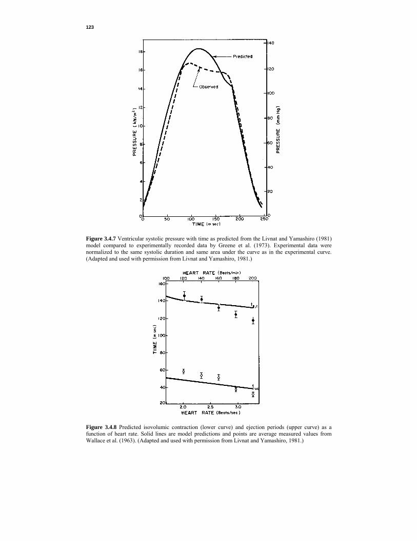
123

Figure 3.4.7 Ventricular systolic pressure with time as predicted from the Livnat and Yamashiro (1981) model compared to experimentally recorded data by Greene et al. (1973). Experimental data were normalized to the same systolic duration and same area under the curve as in the experimental curve. (Adapted and used with permission from Livnat and Yamashiro, 1981.)

Figure 3.4.8 Predicted isovolumic contraction (lower curve) and ejection periods (upper curve) as a function of heart rate. Solid lines are model predictions and points are average measured values from Wallace et al. (1963). (Adapted and used with permission from Livnat and Yamashiro, 1981.)

124

TA

BL

E 3

.4.3

Res

ults

of S

imul

ated

Hea

rt F

ailu

re

Stat

e

End-

Dia

stol

ic

Vol

ume

(Vo),

m

3

(mL)

C

ontra

ctio

n En

ergy

(E2),

N

·m (e

rg)

Max

imal

Rat

e of

Ven

tricu

lar

Pres

sure

Cha

nge

[(dp

/dt) m

ax],

N/(m

2 ·sec)

(mm

Hg/

sec)

Ven

tricu

lar

Elas

tanc

e,

k

N/m

5 (m

m H

g/m

L)

Isov

olum

ic

Con

tract

ion

Perio

d,

sec

Ejec

tion

Tim

e se

c N

orm

al

Mild

dila

tatio

n Se

vere

dila

tatio

n

20

x 1

0-6

30 x

10-6

40

x 1

0-6 (

20)

(30)

(4

0)

36

28

20

(3.6

x 1

0)

(2.8

) (2

.0)

230

x 10

3

181

x 10

3

146

x 10

3 (1

.722

) (1

.356

) (1

.093

)

15

0 x

106

760

x 10

6

490

x 10

6

(11.

6)(5

.7)

(3.7

) 45

x 1

0-3

57 x

10-3

73

x 1

0-3

13

8 x

10-3

147

x 10

-3

154

x 10

-3

Sour

ce: A

dapt

ed a

nd u

sed

with

per

mis

sion

from

Liv

nat a

nd Y

amas

hiro

, 198

1.

125

juxtaposition of concepts: oxygen consumption used to be thought of as a dependent variable-its magnitude was dependent upon the rate of work. This model shows that oxygen consumption can be pictured as determining, at least in part, the rate of work. 3.4.5 Heart Rate Models Heart rate response to exercise is nearly linear. As presented in Equation 3.2.41, steady-state heart rate response can be obtaind from oxygen consumption data by

HR = HRr +

maxO

O

2

2

V

V�

�

( HRmax – HRr) (3.4.24)

where HR = steady-state heart rate response, beats/sec HRr = resting heart rate, beats/sec

2OV� = oxygen uptake, m3 and

HRmax = (220 - y)/60 (3.4.25) where y = age, yr Maximum oxygen uptake can be approximated by any of several empirical predictors such as Equation 3.3.39, 3.2.40, or 3.2.41. Oxygen uptake for any given task can be roughly calculated from other empirical equations (see Section 5.5.1) or by dividing external work rate by an assumed muscular efficiency. For leg work, muscular efficiency can be assumed to be 20% (see Section 5.2.5). Thus steady-state heart rate response to exercise can be predicted approximately. Transient Response. Fujihara et al. (1973a, b) performed a series of experiments in which they were able to determine heart rate transient response. They were careful to begin their experiments at work rates higher than resting and terminate them before maximal efforts, thus avoiding nonlinearities at both extremes of work rates. Five healthy nonathletic laboratory personnel were studied. Impulse, step, and ramp loads were applied to the bicycle ergometer. Good agreement between experimental observations and mathematical prediction was obtained with the following step-response equation (Fujihara et al., 1973a):56

[ ] ( ) ( ) [ ] ( )321 /22

/

12

2/

12

111 111HR τττ δ

τττ

τττδ t

dtt

d ettkeettk −−− −−+

−

−+−

−−

−=∆

(3.4.26) where ∆HR = change in heart rate, beats/sec k1, k2 = steady-state heart rate coefficients, beats/sec td1, td2 = delay times, sec δ[t – td] = 0, t < td = 1, t > td τ1, τ2, τ3 = time constants, sec Experimentally determined parameter values for step changes in work rate of 60 N·m/sec appear in Table 3.4.4. The formulation in Equation 3.4.26 is dominated by a rapid rise in heart 56Actually, Fujihara et al. gave their equation in the s domain (see Appendix 3.3):

( )( )[ ] [ ] 132

1211 111HR 21 −−−− ++++=∆ τττ sekssek dd stst

which does not presuppose any specific type of forcing function such as impulse, step, or ramp. The terms dste

−are time delay

terms and (1 + sτ) terms lead to exponential time responses.

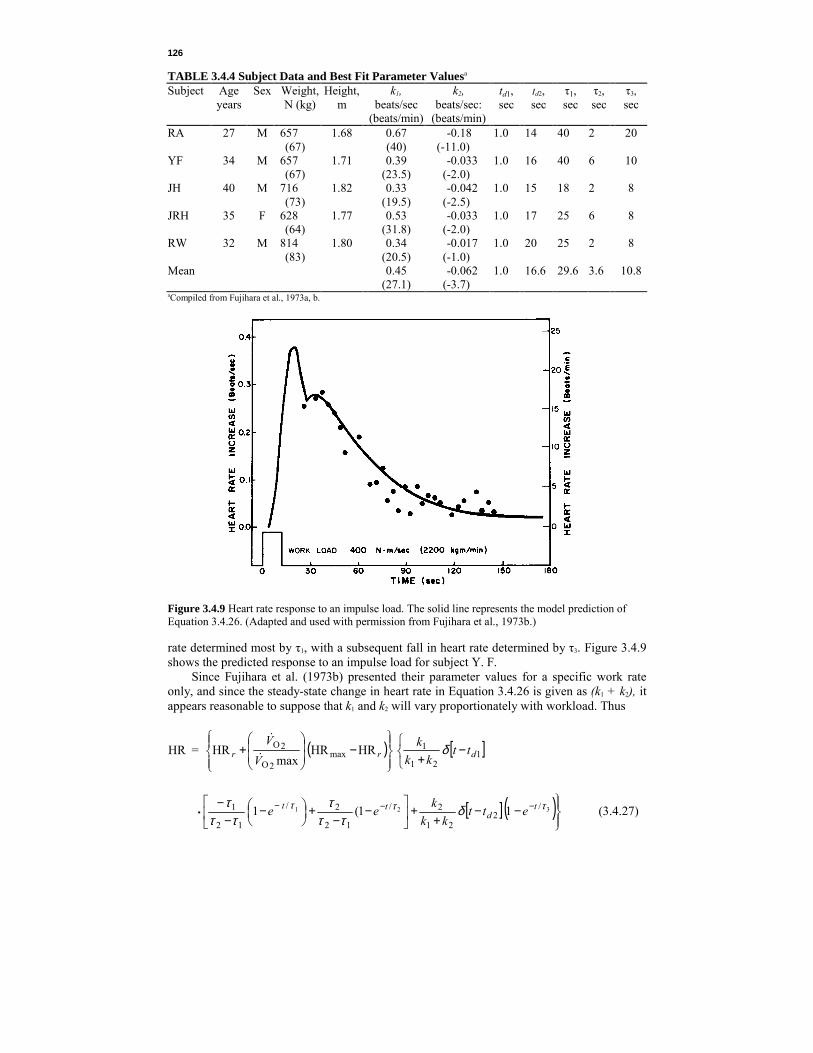
126

TABLE 3.4.4 Subject Data and Best Fit Parameter Valuesa

Subject Age years

Sex Weight, N (kg)

Height,m

k1, beats/sec

(beats/min)

k2, beats/sec:

(beats/min)

td1, sec

td2, sec

τ1, sec

τ2, sec

τ3, sec

RA YF JH JRH RW Mean

27

34

40

35

32

M

M

M

F

M

657 (67) 657 (67) 716 (73) 628 (64) 814 (83)

1.68

1.71

1.82

1.77

1.80

0.67 (40) 0.39

(23.5) 0.33

(19.5) 0.53

(31.8) 0.34

(20.5) 0.45

(27.1)

-0.18 (-11.0)

-0.033 (-2.0) -0.042

(-2.5) -0.033

(-2.0) -0.017

(-1.0) -0.062

(-3.7)

1.0 1.0 1.0 1.0 1.0 1.0

14 16 15 17 20 16.6

40 40 18 25 25 29.6

2 6 2 6 2 3.6

20

10

8

8

8

10.8

aCompiled from Fujihara et al., 1973a, b.

Figure 3.4.9 Heart rate response to an impulse load. The solid line represents the model prediction of Equation 3.4.26. (Adapted and used with permission from Fujihara et al., 1973b.) rate determined most by τ1, with a subsequent fall in heart rate determined by τ3. Figure 3.4.9 shows the predicted response to an impulse load for subject Y. F. Since Fujihara et al. (1973b) presented their parameter values for a specific work rate only, and since the steady-state change in heart rate in Equation 3.4.26 is given as (k1 + k2), it appears reasonable to suppose that k1 and k2 will vary proportionately with workload. Thus

HR = ( ) [ ]

−+

−

+ 1

21

1max

2O

2O HRHRmax

HR drr ttkk

kV

Vδ

�

�

[ ] ( )

−−+

+

−

−+

−−

− −−−• 321 /

221

2/

12

2/

12

1 11(1 τττ δττ

τττ

τ td

tt ettkk

kee (3.4.27)

127

Heat Effects. Heart rate is influenced not only by the oxygen transport requirements of the body but also by body temperature. This reflects the additional cardiovascular burden of removing excess heat (as well as a small increase in oxygen demand to supply the increase in chemical activity which occurs with a temperature increase; see Section 3.3.5 and 5.2.5). Givoni and Goldman (1973a), obtaining experimental observations on young men in military uniforms, proposed a series of equations to predict heart rate response to work, environment, and clothing. For a more thorough discussion of the parameters involved in this model, the reader is referred to Section 5.5. Both body temperature and heart rate respond to environmental changes by transient changes toward new final values. Of course, heart rate changes much more rapidly than body temperature. Figure 3.4.10 shows the relationship between final heart rate for four different studies. The relationship between these two demonstrates the predictability of one from the other. The body temperature model of Section 5.5 corrects body heat load for work done on the external environment by the body.57 No such correction is necessary for heart rate because heart rate responds to total oxygen demand, which includes that used to produce external work. There is a limit above which the relationship between body temperature and heart rate is no longer linear. This limit occurs at a heart rate of about 2.50beats/sec. Above this limit, body temperature can continue to increase (although the subject may expire before equilibrium is reached) while heart rate approaches a maximum of 2.83-3.17 beats/sec. Givoni and Goldman (1973a) assumed an exponential relationship between body temperature and heart rate above this limit. Based on empirical determination, Givoni and Goldman (1973a) gave, for heat-

Figure 3.4.10 Relationship between measured final heart rate and computed equilibrium rectal tempera-ture from four experimental studies. (Adapted and used with permission from Givoni and Goldman, 1973a.) 57External work is work used to move an external force, such as the weight of an object, through some distance.

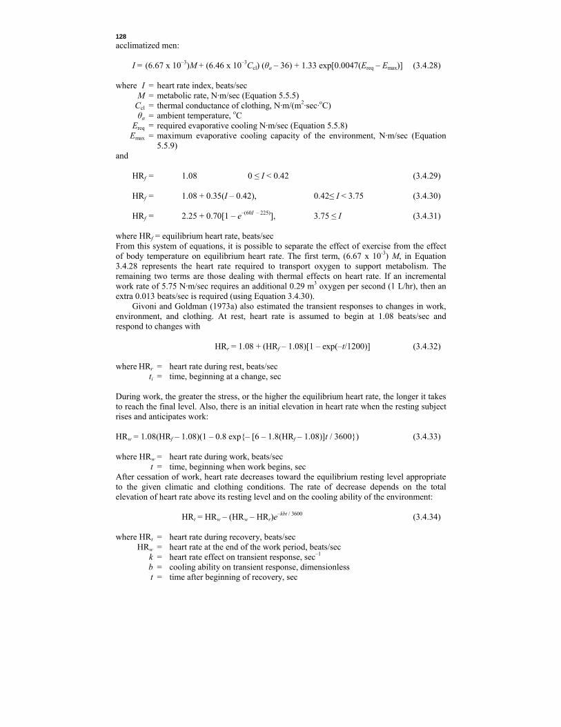
128

acclimatized men: I = (6.67 x 10–3)M + (6.46 x 10–3Ccl) (θa – 36) + 1.33 exp[0.0047(Ereq – Emax)] (3.4.28) where I = heart rate index, beats/sec M = metabolic rate, N·m/sec (Equation 5.5.5) Ccl = thermal conductance of clothing, N·m/(m2·sec·oC) θa = ambient temperature, oC Ereq = required evaporative cooling N·m/sec (Equation 5.5.8)

Emax = maximum evaporative cooling capacity of the environment, N·m/sec (Equation 5.5.9)

and HRf = 1.08 0 ≤ I < 0.42 (3.4.29) HRf = 1.08 + 0.35(I – 0.42), 0.42≤ I < 3.75 (3.4.30) HRf = 2.25 + 0.70[1 – e–(60I – 225)], 3.75 ≤ I (3.4.31)

where HRf = equilibrium heart rate, beats/sec From this system of equations, it is possible to separate the effect of exercise from the effect of body temperature on equilibrium heart rate. The first term, (6.67 x 10-3) M, in Equation 3.4.28 represents the heart rate required to transport oxygen to support metabolism. The remaining two terms are those dealing with thermal effects on heart rate. If an incremental work rate of 5.75 N·m/sec requires an additional 0.29 m3 oxygen per second (1 L/hr), then an extra 0.013 beats/sec is required (using Equation 3.4.30). Givoni and Goldman (1973a) also estimated the transient responses to changes in work, environment, and clothing. At rest, heart rate is assumed to begin at 1.08 beats/sec and respond to changes with HRr = 1.08 + (HRf – 1.08)[1 – exp(–t/1200)] (3.4.32) where HRr = heart rate during rest, beats/sec ti = time, beginning at a change, sec During work, the greater the stress, or the higher the equilibrium heart rate, the longer it takes to reach the final level. Also, there is an initial elevation in heart rate when the resting subject rises and anticipates work: HRw = 1.08(HRf – 1.08)(1 – 0.8 exp{– [6 – 1.8(HRf – 1.08)]t / 3600}) (3.4.33) where HRw = heart rate during work, beats/sec t = time, beginning when work begins, sec After cessation of work, heart rate decreases toward the equilibrium resting level appropriate to the given climatic and clothing conditions. The rate of decrease depends on the total elevation of heart rate above its resting level and on the cooling ability of the environment: HRt = HRw – (HRw – HRr)e–kbt / 3600 (3.4.34) where HRt = heart rate during recovery, beats/sec HRw = heart rate at the end of the work period, beats/sec k = heart rate effect on transient response, sec–1 b = cooling ability on transient response, dimensionless t = time after beginning of recovery, sec