Cardiac Passive Acoustic Localization: Cardiopal

ELEKTRIK, VOL.6, NO.3, 1998, c©TUBITAK

Cardiac Passive Acoustic Localization: Cardiopal

Yıldırım Bahadırlar, Halil Ozcan GulcurBogazici University, Biomedical Engineering Institute,

80815 Bebek, Istanbul-TURKEYTel: (0212) 263 15 40 - 1438/1443, Fax: (0212) 257 50 30

e-mail: [email protected], [email protected]

Abstract

A novel non-invasive system is proposed as an adjunct diagnostic tool for cardiac disorders, which

is based on processing of the heart sounds acquired using a specially designed 2-D passive acoustic

array. In addition to the acoustic array, the system consists of a personal computer, specially developed

instrumentation and interface hardware and an adaptive array processing scheme. A signal model is

constructed in accordance with the basic assumptions made for very near-field low frequency sources. The

multiple signal characterization (MUSIC) method together with the model is used for the localization of

assumed point sources in the heart. Locations of the sources are estimated by applying 2-D searches.

The effectiveness of the system is demonstrated with extensive recordings at different SNR levels on the

phantoms constructed using small sound sources. The system is also tested on human subjects. Different

“images” corresponding to the various phases of the heart beat are obtained. It is explained that extraction

of 3-D “images” is also possible with the same array data by evaluating a distance parameter relating the

sources to the origin of the array.

1. Introduction

The heart, due to its blood pumping action, is one of the most powerful acoustic sources within the body.It emits low frequency vibrations with a rather high dynamic range. Recent experimental and theoreticalstudies have emphasized the importance of distinct structures of the heart tissue in the genesis of the heartsounds. For example, rapidly changing tension of the myocardium, acceleration and deceleration of bloodmasses and valvular activities cause multi-component heart sounds during the cardiac cycle. They act asthe driving forces on the vibratory modes of the surrounding tissue and the myocardium. Moreover, theturbulent flow due to a regurgitation or a stenosis can cause deterministic vibrations of the vessel wallsand the myocardium. When these sounds are recorded on the chest wall, they are also conditioned by thetransmission characteristics of the myocardium, the lung and the thoracic tissue [1-7].

Monitoring the entire region of the heart may require many sensors. Vermarien et al. [8] and Okada etal. [9] successfully obtained low-frequency vibratory maps on the chest wall with contact type transducers.Ramachandran et al. [10] used a capacitance type distance meter to reconstruct 2-D patterns of the cardiacactivity. During various phases of the ECG, they displayed the out-of-plane displacements caused by majorcardiac events in a perspective view. Hok et al. [11] applied a holographic method with pulsed ruby laser toprovide a measurement without any contact. Another optical technique based on laser speckle interferometryhas been developed by Ramachandran et al. [12]. They analyzed the displacements during P, QRS and T

243

ELEKTRIK, VOL.6, NO.3, 1998

segments of the ECG. Recently, several investigators have directed their efforts to achieve a spatial mappingof the acoustical energy emitted by the heart. In these investigations, the heart sounds are acquired fromcertain conventional landmark points on the chest. They are then processed using coherent averaging andinterpolating the acoustic energy among the cardiac sensors [1, 4].

In the present study, a novel system was developed for spatial localization and 2-D mapping ofthe assumed acoustic sources of the heart. The system is called Cardiac Passive Acoustic Localizer orCARDIOPAL, for short. It consists of a specially designed multi-sensor probe in the form of a planarmicrophone array, precision amplifiers, filters and A/D converters, interface circuitry, a PC and software.With this system different ”images” corresponding to the various phases of the heart beat; e.g., closure ofthe mitral and tricuspid valves, ejection of blood flow in the systole, closure of the aortic and pulmonaryvalves, early and late diastole, were obtained. The details of the system and the method used are describedin the following sections.

2. The 2-D Sensor Array and the Instrumentation System

The multi-sensor probe developed is a 105 mm x 105 mm x 40 mm planar acoustic array made with 16miniature electret microphones mounted on a 4 x 4 grid. A soft polyurethane layer was used to couple therigid surface of the collimator of the array to the chest wall. The data acquisition hardware consists ofbalanced microphone amplifiers, 80-1000 Hz band-pass analog filters, Analog-to-Digital Converters (ADC)and an interface to a PC. During data acquisitions all microphone channels are sampled simultaneously andquantized using 12-bits and the acquired data is transferred to the PC via Direct-Memory-Access (DMA).

In the present study, from the signal processing point of view, it is crucial to have an instrumentationsystem for the array with sufficiently low amplifier noise, thus an adequate dynamic range, and a high enoughCommon-Mode-Rejection-Ratio (CMRR). The present system has an average noise factor of 1.0232 and 51.6dB dynamic range (measured when an acoustically isolated microphone is coupled to a channel) and average86 dB (at 50 Hz) CMRR. These specifications of the instrumentation system are quite sufficient for accuratemeasurement of the heart sounds. Further details about the microphone array and the instrumentationsystem are given by Bahadırlar [13].

3. Directional Response of the Array

The construction of the microphone array effectively limits the omnidirectional response of the air-coupledmicrophones and confines its sensitive region to the orifice of the coupling layer. However, the quiescentdirectional response of the array is not suitable to localize vibrating structures within the heart. In otherwords, one cannot differentiate these sites merely by steering the mainlobe of the microphone array. This isdue to the fact that the mainlobe is almost semi-spherical on the chest side, even for the upper frequencyof the instrumentation system (1000 Hz). The dimensions of the array are very small and the frequency ofinterest is rather low [13]. Fortunately, with the help of advanced array processing techniques, the degreesof freedom of the array can be utilized effectively to obtain spatial information beyond that obtained fromthe quiescent directional response of the array [14]. Furthermore, by making judicious assumptions aboutthe hypothetical acoustic sources and about the propagation of the acoustic energy emitted from the hearttissue to the array, spatial differentiation can be achieved.

244

BAHADIRLAR, GULCUR: Cardiac Passive Acoustic Localization: Cardiopal

4. Assumptions about the Heart Sounds

The genesis and propagation of the heart sounds through the transmission system from the heart to thechest surface is a very complex phenomenon and the mechanisms involved are still controversial. The oldesttheory, called the valvular theory states that the heart sounds are actually produced by the opening andthe closure of the four cardiac valves [1]. Another widely accepted cardiohemic theory relates the heartsounds to the vibration of the entire cardiac structures acting as a single body [1, 2]. The theory contains amechanism for the genesis of the heart sounds, incompatible with the valvular theory since it emphasizes theimportance of the whole complex of the heart tissues, and acceleration and deceleration of the blood in theheart. The cardiohemic theory excludes the valve vibration as a cause of the heart sounds. Combining theobservations of the previous theories, a modern theory named the multi-degree of freedom theory states thatintracardiac sounds originate from distinct cardiac structures [1]. This theory hypothesizes that the cardiacstructures differs in morphology, therefore the individual structures contribute to the heart sounds on thebasis of their different vibratory modes. Although the valvular and the cardiohemic theories are partly valid,recent investigations strongly support the multi-degree of freedom theory [1, 3, 7].

The heart-thorax acoustic system acts as a slowly time-invariant low-pass filter. Therefore theintracardiac sounds are also conditioned by this acoustic system. In addition, the frequency content ofthe sounds on the chest surface does not change significantly between different sites on the chest, whereasthe intensity changes considerably and characteristically [1, 7]. Bearing in mind these findings and themulti-degree of freedom theory, the following assumptions for the production and propagation of the heartsounds can be adopted to form a signal model to be occupied in our array processing approach:

• The vibrating tissue is small compared with the size of the microphone array and acts as a point source.Therefore, the sound wave from the tissue is propagated as a spherical wave in this very near field.

• There is no scattering or reflection of the sound wave within the tissue between the heart and the chestsurface.

• The intervening tissue is homogeneous in terms of sound absorption characteristics. The sound velocityis assumed to be constant and can be taken as c = 1530 m/sec.

• The sound sources are stationary within the observation interval of interest.

Considering the difficulty in establishing of a strong theory for the genesis and propagation of theheart sounds, the assumptions may be viewed as controversial. Nevertheless, they will promote the arrayprocessing scheme described in the next section and the performance of the method will be discussed insections 6 and 7 with this signal model and the array data acquired from the human subjects.

5. The Signal Model and Acoustic Source Localization

The MUSIC algorithm is a subspace-based estimation technique in array signal processing and relies on thegeometrical properties of an assumed signal model [15, 16]. If the model accurately represents the measureddata, the algorithm can result in “superresolution”; a capability not limited by the array size, but by thedata collection time and/or the SNR level of the measured data.

245


(m,n)'th microphone

dy

dx 0

x

y

zk'th sound source

rork

dmn

θk

Ok

Figure 1. A point source in the near-field of the 4x4-element planar array.

In the present study, considering the special geometry of the microphone array, a signal model wasdefined in accordance with the assumptions given in Section 4. Figure 1 shows a point source in the nearfield of the array. Its coordinates and its range to the array origin are used as the principal parameters ofthe signal model in Eq. (1) given below. Assuming that there are K point sources in the near field of thearray, the model for the signal Xmn(t) at the microphone in location (m, n) can be written as

Xmn(t) =K∑k=1

Sk(t)amn(t, rok, θk, φk) + nmn(t), 1 ≤ m ≤M, 1 ≤ n ≤ N ; (1)

where Sk(t) is the amplitude of the k’th sound source, amn(t, rok, θk, φk) is the array steering parameterdepending on the location of the k’th source, nmn(t) is spatially white Gaussian noise, M and N are thenumber of microphones in the x and the y axes, respectively. Assuming the near-field sources to be stablein their locations during the observation time, the array steering parameter can be given as:

amn(rok, θk, φk) =

rokdmn(rok, θk, φk)

2

· exp[−(ρdmn(rok, θk, φk)/rok + jk0(rok − dmn(rok, θk, φk)))] (2)

dmn(rok, θk, φk) =[r2ok + x2

m + y2n − 2rok sin θk(xm cos θk + yn sinφk)

]1/2(3)

xm = [m− (M + 1)/2]dx, yn = [n− (N + 1)/2]dy, κ0 = 2πf0/(c/dx), dx = dy,

where rok is the distance between the k’th source and the array origin, dmn(rok, θk, φk) is the distance fromthe same source to the (m, n)′th array element, θk and φk are the elevation and azimuth angles, respectively(see Figure 1), κ0 is the wave number depending on the frequency of the source (f0) and on the speed ofthe sound (c) in the medium, dx and dy are the inter-element distances in the respective axes on the arrayand ρ is the exponential loss factor of the medium.

The steering parameter amn(rok, θk, φk) consists of three factors, two of which correspond to theassumptions given in the preceding section and the other is due to the delay/advance of the wave withrespect to the unmeasured wave at the array center. The first factor represents the intensity loss due to the

246


spherical wave expanding about a point source. The intensity level is inversely proportional to the secondpower of the distance from the source. This is due to the spherical surface of the symmetrically expandingwave. The second factor is due to the energy loss per unit volume in a lossy homogenous medium. If the lossis a constant fraction of the wave energy, the intensity loss caused by the medium is an exponential functionof the distance to the source [17, 18].

The array output can be written as an M ×N column vector X (t) from (1) by arranging the outputsof the rows one after the other. In this case the MN ×MN array output covariance matrix can be given as

R= E[X(t)X H(t)

](4)

where (·)H represents the complex conjugate transpose (Hermitian). If we assume the spatial noise to bestatistically independent among the channels and from the source signals, the covariance matrix can bewritten as

R = ARSA H + σ2I. (5)

where RS represents the source covariance matrix of size K × K,A is the steering matrix of MN × Kelements correspondingly defined by the steering parameters amn(rok, θk, φk), σ2 is the variance of thespatial noise and I is the identity matrix. If the sources are incoherent, then RS remains nonsingular andhas rank K . A is also of rank K due to the linear independence of its columns. Therefore this implies thatthe ARSA H is also of rank K .

Let λ1 ≥ λ2 ≥ . . . ≥ λMN be the ordered eigenvalues of the array covariance matrix R . They are given by

λk =

{µk + σ2 k = 1, 2, . . .Kσ2 k = K + 1, K + 2, . . . ,MN,

(6)

where µk is the eigenvalue of the source in the noiseless case. For any k > K , the following can be writtenfrom (6):

Rvk = λkvk = σ2vk

Rvk = (ARSA H + σ2I)vk

(7)

where vk is the eigenvector corresponding to the eigenvalue, λk of the covariance matrix. It is seen from(7) that the term ARSA Hvk is equal to zero. Since RS is of rank K and A has full column rank K , itfollows from (7) that

A Hvk = 0, K + 1 ≤ k ≤MN. (8)

A fundamental property of the eigenvectors of a correlation matrix is that they are orthogonal to each other.Hence the K eigenvectors span a subspace that is the orthogonal complement of the space spanned by theremaining MN −K eigenvectors. Therefore, it follows from (8) that the MN −K eigenvectors related tothe noise subspace are orthogonal to the K columns of the steering matrix A, and the columns are relatedto the sources in the scene. Thus the peaks of the following function will correspond to the true locations ofthe sources:

247


P (r, θ, φ) =1∑MN

k=K+1

∣∣∣v Hk a(r, θ, φ)

∣∣∣2 (9)

where a(r, θ, φ) is the steering column vector of size MN and r represents the distance from a source tothe array center. Clearly, the parameters of the function in (9) are the spherical coordinates and can beused to describe the location of a sound source in a volume, thus the classical MUSIC algorithm extendsto a three-dimensional version in the present study [19-22]. Obviously, the function P (r, θ, φ) is meaningfulwhen MN ≥ K + 1 and this limits the minimum number of microphones to resolve the total number ofsources in a scene.

When the array covariance matrix R is known exactly and the assumptions about the noise statisticshold, the peaks of the P (r, θ, φ) are guaranteed to correspond to the true locations. Since the peaks or theeigenvectors are always distinct, this estimator can distinguish arbitrarily close acoustic sources. However, alow SNR in the measured signal and any mismatch between the model in (1) and the measured signal fromthe scene, seriously degrade the resolution of the estimator [15, 16, 19, 20]. In practice, the array covariancematrix R can be estimated from the ensemble average of the array outputs as

R =1L

L∑i=1

X(ti)X H(ti) (10)

where L is the number of the samples and X(ti) is the array output vector obtained at the i’th sample.The K principal and MN −K noise eigenvectors (i.e., the signal and noise subspaces) will be determinedfrom the estimated covariance matrix. The accuracy, with which the number of principal eigenvectors aredetermined, and the quality of the estimated subspace are the crucial factors for the success of the MUSICmethod.

The quality of the estimated signal subspace increases with an increase in the number of samples.Similarly, the estimation bias of the source location is inversely proportional to the number of samples;(∝ L−1). The increase in the noise variance also causes an increase in the bias; (∝ σ2), and the estimationvariance has order L−2 dependence to the samples. Furthermore, the bias is strongly dependent on theseparation of the close sources. Hence, two close sources may not be resolved if the estimation bias is high[15, 23]. In the asymptotic case (i.e., the number of samples is very large), for any number of sources, theestimation variance is very close to the Cramer-Rao lower bound as the noise variance approaches zero, i.e.,as the SNR increases [23].

6. Experimental Study and Results

For testing the array data acquisition system and proposed source localization method experimental datawas acquired. A phantom with three sound sources (small headphone capsules) was constructed to simulatethe point sources and to create various scenarios in a relatively controllable environment. The small capsulewhich has a 2 mm orifice behaves like omnidirectional radiators due to the low frequency of interest (around500 Hz) in the experiments. The aperture of a capsule is very small compared with the wavelength of thesound waves (λair =684 mm at c = 342 m/s and f = 500 Hz). The angle of divergence of the waves dependson the sine of the ratio between the wavelength and half of the aperture [18]. In our case, obviously, the angleof divergence is very large, so that the capsules do not have any directional responses and emit sphericalwaves. The sound signals emitted by these sources were recorded in a silent room. Also, the same phantom

248


was placed into a plastic box which was filled with a boiled gelatin-water mixture to mimic the tissue betweenthe heart and the chest wall. Similar signal measurements were performed on the outer surface of the plasticbox. The heart sounds were also recorded from human subjects while the subjects were supine and askedto hold their breaths. All measurements were performed at 4 kHz sampling frequency. As stated abovethe success of the acoustical source localization method totally depends on the SNR level of the measuredarray data, the stability of the sound producing sites during the observations and matching of the signalpropagation model with the signals impinging onto the array. Therefore, the experimental data was used toevaluate the method in real circumstances.

To get array signals with various SNR levels, two sources were driven by 495 Hz and 505 Hz sinusoidalsignals and the intensities were changed for each SNR. The frequencies of the sources chosen were slightlydifferent to prevent possible coherence. The array signals were passed through a 400-600 Hz band-pass digitalfilter to intentionally confine the background noise into a bandwidth similar to that of the weak diastolicsignals carrying diagnostic value. The SNR level was defined as

SNR(dB) = 10 log

[ ∑Li=1

[XS(ti)− XS

]T [XS(ti) − XS

]∑Li=1

[XN(ti)− XN

]T [XN (ti)− XN

]]

(11)

where L is the number of samples, XS(ti) was the array output vector sampled at i’th sample when thesources were active, XS was the mean vector of XS(ti) calculated over L samples, and XN (ti) was thearray output vector sampled at i’th sample when the array output was only due to the instrumentation andthe ambient noise, XN was the mean vector of XN (ti) calculated over L samples. The SNR was estimatedusing L = 4000 samples.

The array signals were then segmented into L samples for each SNR level and the array covariancematrix in (10) was calculated over these samples. The MUSIC algorithm was applied by choosing the numberof sources as K = 2. A source plane was defined on a 40x40 grid (with 2.5 mm x 2.5 mm grid size) at 5cm distal to the array plane, using the parameter r in (9). The distance between the source plane and thearray plane is the actual distance in the measurement setup. The speed of sound (c) in air was chosen as342 m/sec and the exponential loss factor of the medium (ρ) was found by trial and error as approximately0.45, using a signal with a moderate SNR level.

025

5075

100

025

5075

1000

0.5

1

mmmm

Ort

hogo

nalit

y M

easu

re

(a)

025

5075

100

025

5075

1000

0.5

1

mmmm

Ort

hogo

nalit

y M

easu

re

(b)Figure 2. The estimates of two near-field sound sources at (a) 1.9 dB and (b) 27.3 dB SNR and using L=400 snap-

shots. The sources are 5 cm distal to the array plane.

249


Figure 2 presents the two estimates at SNR levels of 1.9 dB and 27.3 dB. The estimates clearlydemonstrate that an increasing purity in the signals helps the MUSIC estimator to resolve the acousticsources easily with this number of samples. Figure 3 shows the dependence of the estimates on the numberof samples at a SNR level of 6.6 dB (L was assigned to 400 and 1600 samples, respectively). In the case of400 samples, the estimator does not resolve the low-power source whereas at 1600 samples the MUSIC givesa good clue to the locations at this impurity level.

025

5075

100

025

5075

1000

0.5

1

mmmm

Ort

hogo

nalit

y M

easu

re

(a)

025

5075

100

025

5075

1000

0.5

1

mmmm

Ort

hogo

nalit

y M

easu

re

(b)

Figure 3. The estimates of two near-field sources at 6.6 dB SNR and using (a) L=400 and (b) L=1600 snapshots.

The sources are 5 cm distal to the array plane.

025

5075

100

025

5075

1000

0.5

1

mmmm

Ort

hogo

nalit

y M

easu

re

(a)

025

5075

100

025

5075

1000

0.5

1

mmmm

Ort

hogo

nalit

y M

easu

re

(b)

Figure 4. Increasing the size of signal-subspace from K=2 to K=5 can improve the spatial spectrum at low SNR

(1.9 dB).

250


025

5075

100

025

5075

100

1

mmmm

Ort

hogo

nalit

y M

easu

re

(a)

025

5075

100

025

5075

100

0.5

1

mmmm

Ort

hogo

nalit

y M

easu

re

(b)

025

5075

100

025

5075

1000

0.5

1

mmmm

Ort

hogo

nalit

y M

easu

re

(c)

025

5075

100

025

5075

1000

0.5

1

mmmm

Ort

hogo

nalit

y M

easu

re

(d)

Figure 5. Three factors in the array steering vector contribute with various degrees to source localization process in

air: (a) Only the phase-shift factor, (b) only the absorption loss and (c) only the spherical spreading factor included

in the steering vector. (d) all factors are included. (K=2, L=800, SNR=20.2 dB).

If the array covariance matrix is estimated from the real measurements, the ordered eigenvalues are alldifferent with probability one [24]. In general they decrease monotonously to a minimum value, thus makingit difficult to determine the size of the signal- or noise-subspaces [24, 25]. In the case where the SNR levelis low, the condition may be more severe, because the high power noise influences the quality of the signal-and noise-subspaces and the condition in (8) may be violated. In this case, an overestimation in the size (K)of signal-subspace may help the MUSIC estimator to improve its resolving capability, since the estimatoruses a uniform average of the norms of the projection of the steering vectors onto the estimated signal ornoise subspaces [15]. However, increasing the size of the signal-subspace results in spurious signal sourceson the spatial spectra. Figure 4 shows the results of the MUSIC estimator in a sample size (L=1600) andat a low SNR (1.9 dB) when the size of the signal-subspace is increased to K = 5. Although the estimator

251


cannot indicate the low-power source in the case K = 2, it can resolve the two sources in the same samplenumber when the subspace size is K = 5. An improvement may still be obtained by increasing the numberof samples to a point determined by the SNR level.

Figure 5 presents the contribution of each factor in the streering vector, a(r, θ, φ) to the estimatesin air at an SNR level of 20.2 dB and L = 800. Once again, the factors are due to the time delay/advance(or phase-shift), spherical-spreading loss and absorption loss. Figure 5.(a) demonstrates that the phase-shiftfactor contributes less to the estimate in the scenario. Figure 5.(b) gives the estimate which is obtained byretaining only the absorption loss factor in the vector. As verified by a better estimate in Figure 5.(c) thespherical spreading loss dominates the other two factors in the near-field. Figure 5.(c) also confirms that thesmall headphone capsules possess the omnidirectional effect. Figure 5.(d) gives an augmented and the bestestimate where the steering vector consists of all three factors.

Figure 6 shows the estimates when all three sources are activated. Although two close sources are notresolved in Figure 6.(a) the flat form of the larger peak seems to indicate the existence of the two sources.This form is usually observed in other scenarios when the number of samples is small at a high SNR levelor when the SNR level is relatively low. Figure 6.(b) shows a gray-scaled version of the estimate in Figure6.(a). This presentation may provide an easy inspection when the unknown scenarios are estimated by thepresent method.

025

5075

100

025

5075

1000

0.5

1

mmmm

Ort

hogo

nalit

y M

easu

re

(a) (b)Figure 6. The estimate and its gray-scaled version when three soruces are activated. The sources are 5 cm distal

to the array plane and K=5, L=3200, SNR=23.2 dB.

Figure 7 presents the MUSIC estimates from the gelatin phantom at high SNR levels. The sourcesin the phantom are 7.5 cm distal to the array plane. The speed of sound is taken as the speed in water;c=1530 m/sec and the absorption loss is determined by trial and error as approximately ρ = 2. In this casethe multi-path arrivals are stronger since the size of the plastic box is small compared the array size and thesource distance, and the acoustic impedances of the gelatin, the plastic and air are quite different from eachother. In contrast to the signals recorded from the phantom in air, it is observed that the signals from thegelatin phantom do not exhibit a systematic variation among the channels of the array. This demonstratesthat strong echoes in the phantom complicate the scenario. Hence, the sources could not be resolved bythe estimator, in spite of a relatively high SNR level. However, the estimate in Figure 7.(b) indicates theexistence of two sources.

252


025

5075

100

025

5075

1000

0.5

1

mmmm

Ort

hogo

nalit

y M

easu

re

(a)

025

5075

100

025

5075

1000

0.5

1

mmmm

Ort

hogo

nalit

y M

easu

re

(b)

Figure 7. The estimates from the gelatin phantom at K=7, L=3200, and (a) at SNR=14.9 dB, (b) at SNR=19.9

dB.

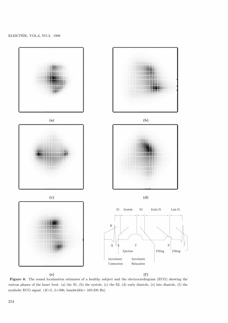
Figure 8 shows the sound localization estimates during the various phases of the heart beats froma healthy subject. Part (f) of the Figure correlates the estimates to the time interval of a representativeECG signal. The heart sounds recorded by the microphone array are segmented by considering the mainphysiological activities at each heart beat. These are the first heart sound (S1), the systole, the second heartsound (S2), early diastole (S3, if it exists) and late diastole (S4, if it exists). The segment length (the numberof samples) in the estimates is L = 500. The array covariance matrix for each phase of the heart beat iscalculated and averaged over the segments from 4 - 5 available beats to increase the quality of the estimates.This may seem to violate our previous assumption that the sound sources must be stationary during theobservation interval since it is well known that the dynamic activities in a phase of the cardiac cycle causes theheart sounds to be nonstationary even in relatively short periods. Nevertheless, in the present study, possiblesound foci are assumed to be stationary during each phase of the beats. The steering parameter in the signalmodel includes a single frequency because of the time delay/advance factor. Therefore, the segments passedthrough a narrow band filter with corner frequency at 165 Hz and 235 Hz (70 Hz band width) to obtainnearly single frequency heart sound signals, and to practically conform to the single frequency property ofthe signal model. The filter is the FIR digital filter with 65 tap weights and constructed using the Chebychevwindow with the ripple level of -40dB at the stop-band region.

The dimensions of the search plane in Figure 8 are assigned for 125 mm x 125 mm for all estimates.Four parameters in the method are then chosen to extract the possible sources in each phase of the heartbeat:

• The speed of sound is assigned to the speed in water; c = 1530 m/sec.

• The absorption loss is determined by trial and error approximately as ρ = 8.

• Number of sources in the scene is determined by trial and error approximately as K = 5.

• The distance of the search plane to the array is changed to get various planes of the estimates.

253


(a) (b)

(c) (d)

(e)

Ejection Filling Filling

Isovolumic Isovolumic

RelaxationContraction

TS

R

PQ

S1 S2Systole Late D.Early D.

(f)

Figure 8. The sound localization estimates of a healthy subject and the electrocardiogram (ECG) showing the

various phases of the heart beat: (a) the S1, (b) the systole, (c) the S2, (d) early diastole, (e) late diastole, (f) the

symbolic ECG signal. (K=5, L=500, bandwidth= 165-235 Hz)

254


The single absorption loss factor in the present study originates from the fundamental assumptionwhich assumes the intervening tissues between the heart and the chest surface are homogeneous in termsof sound absorption characteristics. However, the complex tissue structures make it difficult to extract asingle factor representing the absorption characteristic of the tissues, and a quantitative measurement of thisfactor may need detailed in vitro studies. Therefore, in the present study the absorption loss is determinedby trial and error. It is observed that increasing the loss shrinks the features recognized on the estimatesand decreasing the value of the factor causes the features to widen together with a smoothing effect. Anextreme change in the factor causes all existing features to disappear.

Many observations in the study show that ordered eigenvalues of the array covariance matrices, whichcorrespond to the different phases of the heart beats, do not exhibit any distinct jump, rather they decreasemonotonously to a small value. This basically implies that there are many sound sources in the scene, buriedin the noise. This also does not conflict with the multi-degree of freedom theory accepted as a fundamentalconception in the study. Increasing the number of sources to the maximum value simply gives distinct andsharp sound foci in the estimates, whereas a decreased value of K results in smoothed and widened sourceswhich seem to be more easily correlated to the activities included in a cardiac phase under inspection.Therefore, the absorption loss and the number of sources are determined by making many observations onthe various phases of the beats and by considering the activities in the corresponding phases. The mostuseful values given above are kept constant in the estimates of all cardiac phases.

The first heart sound, during which many cardiac activities take place in the heart, has the mostcomplicated nature among the other heart sounds. Because of this, the estimate for the first heart soundin Figure 8.(a) is quite difficult to interpret. However, the higher acoustic energy in the figure appears torepresent the closure of the mitral valve and early systolic activity in the left heart. Figure 8.(b) presentsthe estimate during the ejection of blood from the left ventricle to the aorta, i.e. the systolic phase. Thisfigure exhibits higher acoustic energy on the left ventricle side and lower energy towards the aortic side. Theacoustic energy due to the closure of the pulmonary and aortic semilunar valves during the end systole andthe second heart sound are clearly seen as two foci in Figure 8.(c). During early diastole the rush of theblood from the left atrium to the left ventricle may be inferred from Figure 8.(d). Figure 8.(e) shows theacoustic energy during the active filling of the left ventricle by the contraction of the left atrium.

Normally, the vibrating sites of the heart do not exhibit very small and discrete sounding foci likeideal point sources, rather they are continuously distributed in a volume of heart tissue. Therefore, one canexpect that the present array data and signal processing method can give a profile of the sounding volumeprojected onto the search plane and the profile may be considered to be composed of very close acousticsources, not resolved due to the limits of the resolution. From this point of view, the estimate in Figure8 can be regarded as a kind of “image” of the vibrating regions, smoothed by the system resolution. Asmentioned above, the heart can be assumed to be a system with a multi-degree of freedom in which theheart sounds are composed of various vibrating structures having different frequency bands [1]. Thus, theestimates in Figure 8 are related to narrow-band vibrations. These ideas lead to the careful interpretationsof Figure 8 when the underlying events in the heart are considered.

Results similar to those in Figure 8 were also obtained for two other human subjects; one healthyand the other diseased, with a weak aortic stenosis and widened aortic root, which were determined byechocardiography examination. Also, the estimates corresponding to the first and the second heart soundsof a prenatal baby (30 weeks old) were achieved. The closure of the four cardiac valves could be demonstratedby utilizing the different estimates with increasing distances of the search plane.

255


(a) (b)

(c) (d)

(e) (f)

Figure 9. The second heart sound estimates from another healthy subject, with respect to the distance from the

array plane: (a) 4 cm, (b) 5 cm, (c) 6 cm, (d) 7 cm, (e) 8 cm, (f) 9 cm. (K=5, L=500, bandwidth=100-400 Hz).

256


Figure 9 shows the estimates for the second heart sound (S2) of the other healthy subject, dependingon increasing distances from the array plane. The sound energy seen on the left side of the estimates inthe figure represents the closure of the pulmonary valve and the energy on the right shows the closure ofthe aortic valve. The figure indicates that the pulmonary valve comes closer to the array plane than theaortic valve. These findings do not conflict with the anatomical placements of the related structures. Theestimates far from the array plane show a blurred version of the sound sources existing near the array asgiven in Figure 9.(e) and Figure 9.(f). This out-of-plane smoothing effect is also observed in the experimentwith the phantoms when the search plane is placed at a distance other than the real distance of the soundsources of the phantoms.

These conclude the principal results obtained from the measured signals. Details and further resultswere given by Bahadırlar [13].

7. Conclusion

In this study, an array signal processing method is proposed for multi-channel heart sound signals. Themethod is totally original in this area and provides acoustic “images” of the heart corresponding to thevarious phases of the heart beat; e.g., closure of the mitral and tricuspid valves, ejection of blood flow duringsystole, closure of the aortic and pulmonary valves, early and late diastole, etc.

Because of physical limitations, the size of the array used is very small compared with the wavelengthof the acoustic waves propagating through the thorax. This makes the directional response of the arrayquite wide and therefore the localization of the acoustic sources within the chest difficult. In spite of thesedifficulties, the proposed method has been successful in the localizations due to the use of “superresolution”array processing techniques together with a judicious choice of the signal model.

The performance of the proposed method depends totally on the amount of uncertainty in the data,i.e., a high SNR in the recorded signal is the key factor for improved resolution. Naturally, the resolutionalso depends on the number of sensors in the array and the quantization depth used in the analog to digitalconversion process. Therefore, a system with more sensors, very low instrumentation noise and a higherquantization depth will have a better overall resolution. A further improvement in the resolution is possibleif a flexible array is used instead of a rigid array. In a rigid array, some of the sensors may not be tightlycoupled to the surface of the chest wall, if the contour of the array does not match closely that of the chest.This may seriously degrade the resolution. In a flexible array the coupling of the sensors could be muchbetter. However, the flexible array must be equipped with the means for monitoring the positions of theindividual sensors with respect to the reference coordinates used in the processing.

The system can also be used to obtain 3-D acoustic “images” of the heart, since the signal modelwith the streering vector defines a three dimensional volume in front of the array in which the localizationprocess can be performed using a single estimate of the array covariance matrix and using 3-D search. Inthis sense, the 3-D estimation is a natural extension of the study. However, the 3-D estimation needs someadditional, surface rendering and shading processes to depict the vibrating sites like physical objects. Inaddition interfering components from the off-place sources should be eliminated. Basic normalizing andthresholding operations defined over the search volume may be used to remove these interferences.

The processing can also be made independent of frequency by neglecting the minor contribution ofthe phase factor in the model, so that the method can directly be used for wide-band estimates of the heartsound signals.

This new imaging modality offered by the proposed system makes it possible to view the heart sounds

257


from a new perspective. The method, visualizing the sound foci of the human heart, employing a depthparameter and relating them to specific frequency bands, can yield a huge amount of valuable, diagnosticinformation from the array data recorded in a short time from a human subject. Our limited experience withthe system shows that it has a good potential of becoming a useful tool for the diagnosis and prescreeningof the cardiac disorders. The potential of this totally noninvasive and safe method must be further exploitedthrough extensive comparative clinical investigations.

8. Acknowledgement

This research was supported by Bogazici University Research Foundation.

References

[1] L-G. Durand and P. Pibarot, “Digital Signal Processing of the Phonocardiogram: Review of the Most Recent

Advancements”, Crit. Rev. Biomed. Eng., Vol. 23, pp. 163-219, 1995.

[2] R.M. Rangayyan and R.J. Lehner, “Phonocardiogram Signal Analysis: A Review”, CRC Crit. Rev. Biomed.

Eng., Vol. 15, No. 3, pp. 211-236, 1988.

[3] J.C. Wood, M.P. Festen, M.J. Lim, A.J. Buda and D.T. Barry, “Regional Effect of Myocardial Ischemia on

Epicardially Recorded Canine First Heart Sound”, J. Appl. Physiol., Vol. 72, pp. 291-302, 1994.

[4] J.C. Wood and D.T. Barry, “Quantification of First Heart Sound Frequency Dynamics Across the Human

Chest Wall”, Med. Bio. Eng. & Comp., Electrocardio., Myocard. Contract. and Blood Fl. Suppl., pp. s71-s78,

July 1994.

[5] J.C. Wood and D.T. Barry, “Time-Frequency Analysis of Skeletal Muscle and Cardiac Vibrations”, Proc. of

the IEEE, Vol. 84, No. 9, pp. 1281-1294, Sept. 1996.

[6] H. Koymen, B.K. Altay and Y.Z. Ider, “A Study of Prosthetic Heart Valve Sounds”, IEEE Trans. on Biomed.

Eng., Vol. 34, No. 11, pp. 853-863, Nov. 1987.

[7] A. Baykal, Y.Z. Ider and H. Koymen, “Distribution of Aortic Mechanical Prosthetic Valve Closure Sound

Model Parameters on the Surface of the Chest”, IEEE Trans. on Biomed. Eng., Vol. 42, No. 4, pp. 358-370,

April 1995.

[8] H. Vermarien, “Construction of Heart Vibration Matrices at 49 Chest Wall Sites by Using Non-simultaneous

Recordings: A Data Acquisition Apparatus and Preprocessing Procedure”, Automedica, Vol. 5, pp. 239-256,

1984.

[9] M. Okada, T. Nakajima, N. Eizuka, Y. Saitoch, and M. Yakata, “Isochronal Map of Chest Wall Vibration with

Cardiokymography”, Comp. Prog. Biomed., Vol. 26, pp. 105-114, 1988.

[10] G. Ramachandran, S. Swarnamani and M. Singh, “Reconstruction of Out-of-Plane Cardiac Displacement

Patterns as Observed on the Chest Wall During Various Phases of ECG by Capacitance Transducer”, IEEE

Trans. on Biomed. Eng., Vol. 38, No. 4, pp. 383-385, 1991.

[11] B. Hok, K. Nilsson, and H. Bjelkhagen, “Image of Chest Motion Due to Heart Action by Means of Holographic

Interferometer”, Med. Biol. Eng. Comp., Vol. 16, pp. 163-168, 1978.

[12] G. Ramachandran and M. Singh, “Three Dimensional Reconstruction of Cardiac Displacement Patterns on the

Chest Wall During P, QRS and T segments of ECG by Laser Speckle Interferometry”, Med. Biol. Eng. Comp.,

Vol. 27, pp. 525-530, 1989.

[13] Y. Bahadırlar, “Cardiopal: Cardiac Passive Acoustic Localization and Mapping using 2-D Recordings of Heart

Sounds”, Ph.D. Thesis, Bogazici University, Biomedical Engineering Institute, Oct. 1997.

258


[14] W.F. Gabriel, “Spectral Analysis and Adaptive Array Superresolution Techniques”, Proc. of the IEEE, Vol.

68, No. 6, pp. 654-666, June 1980.

[15] S. Haykin, Advances in Spectrum Analysis and Array Processing, Prentice Hall, Englewood Cliffs, NJ, 1991.

[16] H. Krim and M. Viberg, “Two decades of Array Signal Processing Research”, IEEE Signal Processing Magazine,

pp. 67-94, July 1996.

[17] W.S. Burdic, Underwater acoustic system analysis, Prentice-Hall Signal Processing Series, Inc., Englewood

Cliff, NJ, 1984.

[18] L.E. Kinsler, A.R. Frey, A.B. Coppens, J.V. Sanders, Fundamentals of Acoustics, John Wiley & Sons, Inc.

Third Edition, NY, 1982.

[19] S. Haykin, Adaptive Filter Theory, 2nd ed., Prentice Hall, Englewood Cliff, NJ, 1991.

[20] S.U. Pillai, Array Signal Processing, Springer-Verlag, NY, 1989.

[21] Y-D. Huang, M. Barkat, “Near-Field Multiple Source Localization by Passive Sensor Array”, IEEE Trans. on

Antennas and Propagation, Vol. 39, No. 7, pp. 968-975, July 1991.

[22] Y-M. Chen, J-H. Lee, C-C. Yeh, “Two-Dimensional Angle-of-Arrival Estimation in the Presence of Finite

Distance Sources”, Trans. on Antennas and Propagation, Vol. 40, No. 9, pp. 1011-1022, July 1992.

[23] B. Porat, B. Friedlander, “Analysis of the Asymptotic Relative Efficiency of the MUSIC algorithm”, IEEE

Trans. on Acoust., Speech and Signal Processing, Vol. 36, No. 4, pp. 532-544, April 1988.

[24] M. Wax and T. Kailath, “Detection of Signals by Information Theoretic Criteria”, IEEE Trans. on Acoust.,

Speech and Signal Processing, Vol. ASSP-33, No. 2, pp. 387-392, April 1985.

[25] M. Wax and I. Ziskind, “Detection of the Number of Coherent Signals by the MDL Principle”, IEEE Trans.

on Acoust., Speech and Signal Processing, Vol. 37, No. 8, pp. 1190-1196, August 1989.

259

Documents

Cardiac Passive Acoustic Localization: Cardiopal