Capturing Risk in Hedge Funds: Moving from Positions to ...docs.edhec-risk.com/EAID-2007/presentations/PM3_RISKMETRICS.pdf · Risk Management Capturing Risk in Hedge Funds: Moving

Risk Management

Capturing Risk in Hedge Funds:Moving from Positions to Strategies

Stéphane Daul

Christopher C. Finger

PD

F processed w

ith CuteP

DF

evaluation editionw

ww

.CuteP

DF

.com

http://www.cutepdf.com

2www.riskmetrics.com 2Risk Management

Questions of a hedge fund investor

BenchmarkingHas a particular manager added value in the past?

Stlye analysisHas a manager produced returns consistent with the views he communicates?

Risk forecastingWhat are the potential losses my portfolio could experience in the future?

Portfolio constructionHow do I allocate to managers to implement the bets I would like to make?

Hedge fund replicationAre there more efficient (less expensive) ways to achieve similar risk/return profiles to standard hedge funds?

What do we want to get out of a model?

We will focus on the first three of these.


Modeling choices

Position-basedLarge data demands

Most accurate for risk forecasting if horizon is small relative to portfolio turnover

Useful for style analysis, difficult for benchmarking

Return-based, factorsRisk forecasts require that regression relationships are stable.

Useful for style analysis if factors are representative of styles

Investable factors may be used as benchmarks.

Return-based, statisticalLimited data demands

Attractive for risk forecasting if no data is available, or if turnover is high relative to risk horizon

Not useful for style analysis or benchmarking

What are the different ways to describe hedge funds or portfolios?

Different models are appropriate for different goals.


Agenda

Out-of-sample testing of simple factor modelsSurely, we can do better.

But, factors do enable us to ask specific questions.

Specific factors … the carry trade strategyDistinction between positions and strategies

What have exposures to carry trades been recently?

Specific factors … merger arbitrage strategiesMerger arbitrage as a distinct risk profile

Analyzing individual and portfolio bets

Creating a factor and assessing exposure

Statistical modelStatistical features of hedge fund returns

Modeling the time dynamics

Constructing portfolio distributions


Agenda






Analyzing individual bets






Look at out-of-sample performance

Look at funds in the combined Barclay database with history for 2000-2005

(~1200 funds)

For each set of indices, perform the following exercise:Regress HF returns on indices over last 24 months.

Assume perfect foresight on indices, and forecast next month’s HF return.

Compute error versus realized HF return.

Average errors (out-of-sample residuals) across all HF.

Track errors through time.

If different indices are equally forecastable, then the sizes of out-of-sample

residuals tell us which indices are best for risk estimates.


Average goodness-of-fit in sample

2000 2001 2002 2003 2004 2005 200635

40

45

50

55

60

65

70

R2 (

%)

HFRIEDHECHFRXstatistical


Out-of-sample residuals

2000 2001 2002 2003 2004 2005 20061

1.5

2

2.5

3

3.5

4

4.5

5

5.5P

redi

ctio

n er

ror

(%)

HFRIEDHECHFRXstatistical


Average HF volatility

2000 2001 2002 2003 2004 2005 20062

2.5

3

3.5

4

4.5

5

5.5

6M

onth

ly v

olat

ility

(%

)


Agenda






Analyzing individual bets






The yen carry trade unwind

The tradeBorrow yen at (low) Japanese rates.

Invest in higher rates in another currency.

Collect the interest rate differential (carry) as long as things stay the same.

Lose if JPY strengthens relative to investment currency.

The (hypothetical?) Great Unwind ScenarioJapanese economy strengthens, Bank of Japan raises interest rates.

Yen appreciates.

Traders unwind carry trade, buying yen to pay back financing.

Yen appreciates more.

More traders unwind carry trade, buying yen to pay back financing.

Yen appreciates more.

Etc.


Two big questions

How much am I exposed to the Great Unwind Scenario?

How big is the carry trade, or in other words, how likely is the Great Unwind

Scenario?


Don’t historical stress tests answer the first question?

Prior large yen carry trade unwinding in the aftermath of LTCM.USD-JPY rate moved from ¥134 (5 Oct 1998) …

to ¥117 (9 Oct 1998) …

to ¥110 (11 Jan 1999).

But, this was precipitated by general need to reduce leverage, not specific

Japanese economic news.

Moreover, especially for the longer move (30% over three months), we should

considerTraders’ behavior during this time, and

How much prevailing carry offsets the currency move.

Instantaneous shocks to static positions do not tell us the whole story.


Are we exposed to a position or a strategy?

Build a NAV time series for a simple carry trade strategy.1. Start with $100.

2. Each week, invest a (fixed) proportion of current NAV into a three-month USD deposit. Set proportion to achieve leverage of four.

3. Fund by borrowing in JPY.

4. Hold each position to maturity.

5. Reinvest all proceeds. Calculate NAV daily by marking all positions.

Volatility-based strategy. Similar but …1. Choose maturity and leverage based on carry-to-risk ratio.

2. Close positions weekly.

3. Set parameters to achieve average leverage of four.


Exchange rate and three-month interest differential

Mar98 Sep99 Mar01 Sep02 Mar04 Sep05 Mar07

100

200

300

400

500

600

700

3−m

onth

spr

ead

(bp)

110

120

130

140

150

JPY

per

US

D


Carry-to-risk ratio (three-month maturity)


10

20

30

40

50

60

70

80


Performance of two carry trade strategiesBoth correlated 90% to exchange rate


50

100

200

500

Car

ry s

trat

egy

valu

e

Const matVol−based

124 bp/month

13 bp/month


Historical stress tests

30%24%28%9%-217-Aug-0722-Jun-07

29%22%33%10%6517-May-0606-Dec-05

13%41%52%15%-101-Apr-0404-Aug-03

28%42%52%15%-315-Jul-0208-Feb-02

45%47%74%21%10103-Jan-0019-May-99

28%58%49%14%309-Oct-9805-Oct-98

46%72%100%30%-6411-Jan-9911-Aug-98

Vol-based

Const.

maturityInst. shock

JPY

apprec.

Carry

change EndStart



30%24%28%9%-217-Aug-0722-Jun-07

29%22%33%10%6517-May-0606-Dec-05

13%41%52%15%-101-Apr-0404-Aug-03

28%42%52%15%-315-Jul-0208-Feb-02

45%47%74%21%10103-Jan-0019-May-99

28%58%49%14%309-Oct-9805-Oct-98

46%72%100%30%-6411-Jan-9911-Aug-98

Vol-based

Const.

maturityInst. shock

JPY

apprec.

Carry

change EndStart

Big currency move, but over a long time, while

carry increased



30%24%28%9%-217-Aug-0722-Jun-07

29%22%33%10%6517-May-0606-Dec-05

13%41%52%15%-101-Apr-0404-Aug-03

28%42%52%15%-315-Jul-0208-Feb-02

45%47%74%21%10103-Jan-0019-May-99

28%58%49%14%309-Oct-9805-Oct-98

46%72%100%30%-6411-Jan-9911-Aug-98

Vol-based

Const.

maturityInst. shock

JPY

apprec.

Carry

change EndStart

Volatility rose in advance of JPY appreciation. Second strategy

had reduced positions.



30%24%28%9%-217-Aug-0722-Jun-07

29%22%33%10%6517-May-0606-Dec-05

13%41%52%15%-101-Apr-0404-Aug-03

28%42%52%15%-315-Jul-0208-Feb-02

45%47%74%21%10103-Jan-0019-May-99

28%58%49%14%309-Oct-9805-Oct-98

46%72%100%30%-6411-Jan-9911-Aug-98

Vol-based

Const.

maturityInst. shock

JPY

apprec.

Carry

change EndStart

Carry-to-risk ratio at historical low. Small loss on

vol-based strategy



30%24%28%9%-217-Aug-0722-Jun-07

29%22%33%10%6517-May-0606-Dec-05

13%41%52%15%-101-Apr-0404-Aug-03

28%42%52%15%-315-Jul-0208-Feb-02

45%47%74%21%10103-Jan-0019-May-99

28%58%49%14%309-Oct-9805-Oct-98

46%72%100%30%-6411-Jan-9911-Aug-98

Vol-based

Const.

maturityInst. shock

JPY

apprec.

Carry

change EndStart

Even with higher volatility, the move looked like a surprise, and vol-based

strategy underperformed.


Stress testing concluding thoughts

It is important to consider whether we are exposed to a position or a strategy,

especially if the events we worry about are likely to occur over a long

timeframe. This can impact which historical events appear to be the most

damaging.

Strategy assumptions are crucial, especially as related to liquidity. We might

further ask the question of how the volatility-based strategy would react if it

took longer to turn over positions.


How much should we worry?How large is the carry trade?

Part of the difficulty is that it is not obvious what is and isn’t a yen carry trade.

Look at proxies for position quantities:JPY futures on the IMM

Peaked in January, dropped in April, peaked in May

BIS statistics on JPY borrowingHeavy activity in 2005, less now

Our approach – examine hedge fund returnsIf HF returns are unusually dependent on the carry trade, there are more positions likely to be unwound quickly if a catalyst event occurs.

Rolling 24-month regressions of HF indices against standard factors (LehmanAggregate, Lehman HY, EMBI+) and one (at a time) carry trade strategy

Carry trade strategies are all vol-based. All finance in JPY. Investment currencies are: USD, AUD, BRL, TWD.


Regressions show a consistent historical dependence on the carry trade, but different pictures today.

Feb00 Apr01 Jun02 Aug03 Oct04 Dec05 Feb07−0.8

−0.4

0

0.4

0.8Market Timing

USDAUDBRLTWD

Feb00 Apr01 Jun02 Aug03 Oct04 Dec05 Feb07−0.8

−0.4

0

0.4

0.8Fixed Income Total


Focus on regression results for 2007.Dependence is increasing, but still is not uniformly positive.

Jan07 Feb07 Mar07 Apr07 May07 Jun07 Jul07 Aug07−0.8

−0.4

0

0.4

0.8Market Timing

USDAUDBRLTWD

Jan07 Feb07 Mar07 Apr07 May07 Jun07 Jul07 Aug07−0.8

−0.4

0

0.4

0.8Fixed Income Total

2

Merger Arbitrage Strategy

1

2

Cash Deal Example

August 8, 2005 QuestDiagnostic Inc. offered$43.90 in cash for eachpublicly held share ofLabOne Inc.

August 9, 2005 the sharesclosed at $42.82 yielding aspread of $1.08

Nov 1st, 2005 the deal wasclosed successfully 31−May−05 31−Jun−05 31−Jul−05 31−Aug−05 30−Sep−05 31−Oct−05

34

36

38

40

42

44

46

Date

Sha

re P

rice

2

2

Equity Deal Example

December 20, 2005 SeagateTechnology announced thatit it would acquire MaxtorCorp. for a fixed shareexchange ratio of 0.37

On December 21, Maxtorshares closed at $6.9 andSeagate at $20.21 yielding a$0.58 merger spread

The deal was completed onMay 22, 2006

31−Oct−05 31−Dec−05 28−Feb−06 30−Apr−06 31−May−063

4

5

6

7

8

9

10

11

Date

Sha

re P

rice

3

2

Withdrawn Deal Example

June 13, 2005, Vin Gupta &Co LLC offered $11.75 incash for each share ofinfoUSA Inc.

After the announcement theshare price of infoUSAjumped to that level

August 24, 2005 the offerwas withdrawn and the shareprice plunged to a similarpre-announcement level

9−Jun−05 31−Jun−05 31−Jul−05 31−Aug−05 30−Sep−058

8.5

9

9.5

10

10.5

11

11.5

12

12.5

13

Date

Sha

re P

rice

4

2

Traditional Model Fallacy

Volatility of the share price before and after theannouncement is very different

31−May−05 31−Jun−05 31−Jul−05 31−Aug−05 30−Sep−05 31−Oct−05Date

Sha

re P

rice

Measuring the risk with a traditional VaR approach in termsof equity volatility is surely wrong

5

2

Merger Arbitrage Risk Model

St stock price at time t

t0 annoucement date

St0 stock price atannouncement

K bid price

∆ merger spread

Λ deal length

t0 + Λ effective date31−May−05 31−Jun−05 31−Jul−05 31−Aug−05 30−Sep−05 31−Oct−05

Date

Sha

re P

rice

St0

K

t0

∆

Λ

6

2

Merger Arbitrage Risk Model

π probability of deal success

Deal completion indicator

C =

{1 with probability = π0 with probability = 1− π

At effectiveness (deal completed or withdrawn)

St0+Λ =

{K if C = 1

S̃t0+Λ if C = 0

Virtual Stock Price

dS̃t = µS̃tdt + σS̃tdWt − I δ (t − (t0 + Λ)) S̃tdt

I ∼ Exp(λ)

7

2

Virtual Stock Price

For t < t0 + Λ, S̃t = St0e∆Z

For t = t0 + Λ, S̃t0+Λ = St0e∆Z (1− I )

31−Sep−05 31−Dec−05 31−Mar−06 30−Jun−06 30−Sep−06 30−Nov−0621

22

23

24

25

26

27

28

29

30

31

Date

Sha

re P

rice

−ISt

8

2

Backtest

Historical estimation

- 41 Merger Arbitrage from HFR database- Monthly performances

VaR level 1st quartile median 3rd quartile95% 0.81% 1.29% 1.68%99% 2.17% 2.92% 4.90%

Monte-Carlo simulation

- 30 cash deals pending in 2006- π = 85%

VaR level Merger Arb Model Traditional Equity Model95% 1.37% 7.25%99% 2.21% 10.24%

9

2

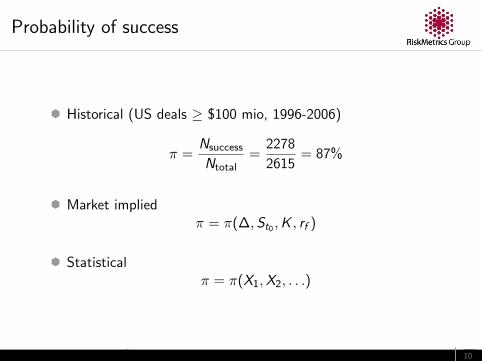
Probability of success

Historical (US deals ≥ $100 mio, 1996-2006)

π =Nsuccess

Ntotal=

2278

2615= 87%

Market impliedπ = π(∆,St0 ,K , rf )

Statisticalπ = π(X1,X2, . . .)

10

2

Cumulative Accuracy Profile

Sort the deals in ascendingorder of probability of success

CAP curve is cumulative ratio offailures as a function ofcumulative ratio of all deals

Ndeals = 100

Nfailures = 10

x = 5% → Nfailures = 3

cap(5%) = 0.3 0 0.1 0.2 0.3 0.4 0.5 0.6 0.7 0.8 0.9 10

0.1

0.2

0.3

0.4

0.5

0.6

0.7

0.8

0.9

1

ratio

CA

P

random

ordered

11

2

Cumulative Accuracy Profile

In-sample : 403 deals

Out-of-sample : 207 deals

0 0.2 0.4 0.6 0.8 10

0.2

0.4

0.6

0.8

1

OOS implied

12

2

Index Construction

Cleaned cash and equity deals

Cash deal daily return

rt =Tt

Tt−1− 1

Equity deal daily return

rt =ρA0e

r(t−t0) + Tt − ρAt

ρA0er(t−1−t0) + Tt−1 − ρAt−1− 1

where

r : short term interest rateρA0 : initial short position in acquirer stock

13

2

Index Construction

From daily returns to monthly returns

From individual deals to index

N deals available at time tNo more than 10% of capital in each deal

wi = min(1/N, 0.1)

wcash = 1−∑

i

wi

14

2

Style Analysis

rD : completed deals

rW : withdrawn deals

rC : cash

rHF ≈∑α

wαrα∑α

wα = 1

1999 2000 2001 2002 2003 2004 2005 20060

0.1

0.2

0.3

0.4

0.5

0.6

0.7

0.8

0.9

1

completedwithdrawncash

15

2

Conclusion

Simple merger arbitrage model

- probability of success- virtual stock price

Validation of main hypothesis

Risk measurement (VaR, stress tests,. . . )

Probability of success

- market implied- statistical model

Index

16

2

Statistical Model

17

2

Introduction

P&L distribution forecasting

Input

- monthly performances- various strategies

Output

- VaR- Risk contribution

18

2

Data

HFR database

Monthly return at time t

rt =NAVt −NAVt−1

NAVt−1

considered net of all hedge fund’s fees

NAVt = net asset value per share at time t

Last reporting date 31-Jul-2007Total number of HF 7041Number of HF older than 10 years 680

19

2

Statistical Tests

Non-normality

Total number of HF 680

Jarque-Bera 598Lilliefor 498

Asymmetry

Total number of HF 680

Wilcoxon 26

20

2

Return-Return lagged correlation

ρ(rt , rt−1)

−1 −0.5 0 0.5 10

10

20

30

40

50

60

70

80

90

Valuation issues

Trading strategy

Smoothing

21

2

Volat-Volat lagged correlation

ρ(σt , σt−1)

−1 −0.5 0 0.5 10

10

20

30

40

50

60

70

80

90

Volatility of volatility

Example

Jan−93 Jan−00 Jul−08−0.2

−0.15

−0.1

−0.05

0

0.05

0.1

0.15

0.2

22

2

Volat-Return lagged correlation

ρ(σt , rt−1)

−1 −0.5 0 0.5 10

10

20

30

40

50

60

HF manager adapts his strategy in downward or upwardmarkets

ρ > 0 : ∆rt−1 > 0 → ∆σt > 0

23

2

Characteristics

Abnormal

- Bulk of return distribution is not asymmetric

- Tail events

Dynamical

- Return autocorrelation

- Heteroscedasticity

- Correlation between return and following volatility

24

2

The univariate process

rt+1 = αrt + σtεt

α : autocorrelation

εt : innovationsE [εt ] = 0, E [ε2t ] = 1

non-normally distributed, e.g. asymmetric-t

σt : dynamical volatility (A-GARCH)

σ2t = ω∞σ2

∞ + (1− ω∞)σ̃2t

σ̃2t = µσ̃2

t−1 + (1− µ) [1− λ sign(rt)] r2t

25

2

Parameter estimation

Parametrization was chosen such that some parameters arethe same for all HF

Parameter Effect captured

α auto-correlation individual ρ(rt , rt−1)ω∞ vol of vol universal 0.55σ∞ long term vol individual std(r)τ vol decay time universal 6λ dynamical asymmetry individual MLEr̄ average return individual mean(r)

ν innovation tails universal 5λ′ innovation asymmetry individual MLE

26

2

Residuals

Forecast for the return and volatility

r̂t+1 and σ̂t

Realized returnrt+1

Realized residuals

εt =rt+1 − r̂t+1

σ̂t

27

2

Univariate tails

Plot log(cdf(ε)) as a function of log(−ε)

{εi ,t}i=1,...,680,t=1,...,60 → {εk}k=1,...,60×680

−1 −0.5 0 0.5 1 1.5 2−16

−14

−12

−10

−8

−6

−4

−2

0

log(−x)

log(

cdf)

residuals t

5

normal

28

2

Backtest

The probtilezt = t5 (εt)

should be uniformly distributed through time and across HF

Relative exceedance

δ(z) = cdfemp(z)− z

0 0.1 0.2 0.3 0.4 0.5 0.6 0.7 0.8 0.9 10

0.1

0.2

0.3

0.4

0.5

0.6

0.7

0.8

0.9

1

29

2

Backtest

Quantification using the metric

d =

∫ 1

0dz |δ(z)|

0 0.02 0.04 0.06 0.08

AR(1) AGARCH asym. t

AR(1) AGARCH t

AR(1) GARCH t

AR(1) GARCH normal

AR(1) normal

AR(0) normal

30

2

Multivariate model

Individual HF process:

AR(1) - AGARCH and t5-innovations

Dependence structure on innovations εi ,t

Extend correlation matrix using copula

F (ε1, ε2) = C [t5(ε1), t5(ε2)]

Capture tail dependency of each strategy

31

2

Tail dependency

Two hedge funds monthly performances

31−Jan−85 31−Oct−87 31−Jan−00−0.5

−0.4

−0.3

−0.2

−0.1

0

0.1

0.2

32

2

Non-parametric estimation

e.g. Fixed-Income Arbitrage

0 0.1 0.2 0.3 0.4 0.5 0.6 0.7 0.8 0.9 10

0.1

0.2

0.3

0.4

0.5

0.6

0.7

0.8

0.9

1

λd = limq→0

P[X ≤ F−1

X (q)|Y ≤ F−1Y (q)

]0 0.005 0.01 0.015 0.02 0.025 0.03 0.035 0.04 0.045 0.05

−0.05

0

0.05

0.1

0.15

0.2

0.25

0.3

0.35

0.4

q

λ

33

2

Tail dependency coefficients

Empirical Empirical ParametricStrategy N Lower Upper λ± σλ νcop

Convertible Arbitrage 16 0.2 0.1 0.18 ± 0.09 6Distressed Securities 18 0.06 0.05 0.05 ± 0.09 10Emerging Markets 29 0 0 0.07 ± 0.06 8Equity Hedge 103 0.05 0 0.04 ± 0.05 10Equity Market Neutral 16 0.04 0.04 0.02 ± 0.03 9Equity Non-Hedge 32 0.1 0 0.17 ± 0.06 5Event-Driven 38 0.17 0 0.11 ± 0.08 7Fixed Income 28 0.09 0 0.03 ± 0.07 9Foreign Exchange 14 0 0.1 0.03 ± 0.09 10Macro 27 0 0.05 0.03 ± 0.08 10Managed Futures 58 0 0.07 0.05 ± 0.07 9Merger Arbitrage 10 0 0.15 0.20 ± 0.17 5Relative Value Arbitrage 20 0.1 0 0.04 ± 0.09 10Short Selling 7 0 0 0.50 ± 0.22 3

34

2

Aggregation with other assets classes

Grouped-t copula

Example

Asset weight iVaR iOmega

Lehman Agg. 40% 1.21 -0.23S&P 500 40% 13.8 0.19

Long-Short 5% 0.31 0.011Merger Arb 5% -0.39 0.035Rel. Value 5% -0.03 0.005Short Seller 5% -1.45 0.08

Total 100% 13.4 0.51

35

2

Conclusion

HF characteristics (abnormality, dynamics, . . . ) can becaptured by a univariate stochastic process with fewparameters to estimate

Out-of-sample backtests are compelling

Multivariate extension using grouped-t copula (simulation aseasy as normal random variate)

All frequencies of data can be mixed (daily, weekly,monthly,...)

Can be aggregated to any other asset class

36

Documents

Capturing Risk in Hedge Funds: Moving from Positions to ...docs.edhec-risk.com/EAID-2007/presentations/PM3_RISKMETRICS.pdf · Risk Management Capturing Risk in Hedge Funds: Moving