Capital Structure and the Informational Role of Debt ...ecsocman.hse.ru/data/871/126/1231/harris_raviv_-_cs_ai_1990.pdf · Capital Structure and the Informational Role of Debt Milton

Capital Structure and the Informational Role of Debt

Milton Harris; Artur Raviv

The Journal of Finance, Vol. 45, No. 2. (Jun., 1990), pp. 321-349.

Stable URL:

http://links.jstor.org/sici?sici=0022-1082%28199006%2945%3A2%3C321%3ACSATIR%3E2.0.CO%3B2-N

The Journal of Finance is currently published by American Finance Association.

Your use of the JSTOR archive indicates your acceptance of JSTOR's Terms and Conditions of Use, available athttp://www.jstor.org/about/terms.html. JSTOR's Terms and Conditions of Use provides, in part, that unless you have obtainedprior permission, you may not download an entire issue of a journal or multiple copies of articles, and you may use content inthe JSTOR archive only for your personal, non-commercial use.

Please contact the publisher regarding any further use of this work. Publisher contact information may be obtained athttp://www.jstor.org/journals/afina.html.

Each copy of any part of a JSTOR transmission must contain the same copyright notice that appears on the screen or printedpage of such transmission.

The JSTOR Archive is a trusted digital repository providing for long-term preservation and access to leading academicjournals and scholarly literature from around the world. The Archive is supported by libraries, scholarly societies, publishers,and foundations. It is an initiative of JSTOR, a not-for-profit organization with a mission to help the scholarly community takeadvantage of advances in technology. For more information regarding JSTOR, please contact [email protected].

http://www.jstor.orgSun Oct 21 09:14:52 2007


http://www.jstor.org/about/terms.html

http://www.jstor.org/journals/afina.html

THE JOURNAL OF FINANCE VOL. XLV, NO. 2 JUNE 1990


MILTON HARRIS and ARTUR RAVIV*

ABSTRACT

This paper provides a theory of capital structure based on the effect of debt on investors' information about the firm and on their ability to oversee management. We postulate that managers are reluctant to relinquish control and unwilling to provide information that could result in such an outcome. Debt is a disciplining device because default allows creditors the option to force the firm into liquidation and generates information useful to investors. We characterize the time path of the debt level and obtain comparative statics results on the debt level, bond yield, probability of default, probability of reorganization, etc.

THEPURPOSE OF THIS paper is to provide a theory of capital structure based on the effect of debt on investors' information about the firm and on their ability to oversee management. We contend that, in general, managers do not always behave in the best interests of their investors and therefore need to be disciplined. Debt serves as a disciplining device because default allows creditors the option to force the firm into liquidation. Moreover, debt also generates information that can be used by investors to evaluate major operating decisions including liqui-dation. The informational consequences of debt are twofold. First, the mere ability of the firm to make its contractual payments to debtholders provides information. Second, in default management must placate creditors to avoid liquidation, either through informal negotiations or through formal bankruptcy proceedings. This process, although costly, disseminates considerable information to investors. Based on the information generated, default can result in major changes in operating policy (including liquidation) and reorganization of the financial structure (see, e.g., Haugen and Senbet (1978) and Bulow and Shoven (1978)).l

* Harris is the Chicago Board of Trade Professor of Finance and Business Economics, Graduate School of Business, University of Chicago. Raviv is the Alan E. Peterson Professor of Finance, Kellogg Graduate School of Management, Northwestern University, and Professor, Faculty of Management, Tel Aviv University. We are grateful to the National Science Foundation and the Bradley Foundation for financial support. Harris would also like to thank Dimensional Fund Advisors for additional financial support. Helpful comments from participants a t seminars a t the University of Chicago, Stanford University, MIT and the 1989 European Economic Association Meetings, especially George Constantinides, Doug Diamond, Allan Kleidon, John Persons, Cynthia Van Hulle, Robert Vishny, and Yoram Weiss are gratefully acknowledged. We also thank Ren6 Stulz, the editor, and an anonymous referee for valuable suggestions.

'The recent financial difficulties of Campeau Corp. provide an example of this process. In return for a $250 million loan that was used to avoid defaulting on existing debt, Olympia and York, another Canadian firm, demanded and obtained a central role in setting Campeau's operating policy.

322 The Journal of Finance

This suggests that, if investors are uncertain about the quality of management and the efficacy of business strategy, they can use debt to generate information about these aspects (see Jensen (1989)) and to obtain a say in setting operating policy. Moreover, the amount and usefulness of the information generated depends on the schedule of debt payments, both timing and quantity. Conse- quently, stockholders will design debt payments, i.e., capital structure over time, at least in part to exploit the ability of debt to generate useful information.

This role for debt has not been investigated in the literature on capital structure. Capital structure theories have focused on the tax advantages of debt (starting with Modigliani and Miller (1963)), the choice of debt level as a signal of firm quality (starting with Ross (1977) and Leland and Pyle (1977)), the use of debt as an antitakeover device (Harris and Raviv (1988)), agency costs of debt (Jensen and Meckling (1976) and Myers (1977)), and the advantage of debt in restricting managerial discretion (Jensen (1986)). While we do not deny the importance of any of these roles for debt in a capital structure theory, we believe that the informational and disciplining role is important and enables us to address issues such as liquidation vs. reorganization that were not addressed in the theories just mentioned.'

A related literature is that concerned with deriving debt as an optimal contract. In Townsend (1979), Diamond (1984), and Gale and Hellwig (1985), managers are presumed to be able to appropriate to themselves any income not paid out while investors are unable to observe income. (In Townsend and Gale and Hellwig, income is observable if a "verification cost" is paid.) These approaches do not allow for outside equity, default without liquidation, or the evolution of debt payments over time. Chang (1987) extends the Townsend model to two periods and allows investors to observe a noisy estimate of income. This makes possible outside equity but does not address the liquidation-reorganization decision. Moreover, Chang does not characterize the evolution of debt payments over time to the extent we do. Finally, Hart and Moore (1989) also provide a dynamic model of debt which distinguishes between default and liquidation. They examine the implications of the ability of creditors to seize assets when debtors default for the form of the debt contract and the efficiency of the debtor-creditor relationship.

This paper offers a theory of capital structure based on the idea that debt allows investors to discipline management and provides information useful for this purpose. In our model, investors use information about the firm's prospects to decide whether to liquidate the firm or continue current operations. We postulate that managers are reluctant to liquidate the firm under any circumstances and are unwilling to provide detailed information to investors that could result in such an outcome. Consequently, investors use debt to generate infor-

A related paper by Titman (1984) also argues that capital structure can be used to improve the liquidation decision. Titman focuses on the failure of stockholders to take account of the costs of liquidation on customers, workers, and suppliers. In the absence of incentives to the contrary, this externality results in liquidation in some situations where it is not socially optimal. Titman argues that debt can serve as a bonding device to encourage continuation in some of these circumstances. We emphasize the opposite agency problem, namely that managers tend to hang on even when they should liquidate. This leads to a different role for debt as described previously.

Capital Structure and the Informational Role of Debt 323

mation and monitor management. They gather information from the firm's ability to make payments and from a costly investigation in the event of default. Debtholders use their legal rights to force management to provide information and to implement the resulting efficient liquidation decision. The optimal amount of debt is determined by trading off the value of information and opportunities for disciplining management against the probability of incurring investigation costs.

We develop both static and dynamic models. In the static model, we consider a once-and-for-all choice of debt level. In the dynamic model, we examine the evolution of capital structure and net payments to debtholders over time. We address the implications of our model for capital structure as well as such issues as what determines liquidation vs. reorganization, how capital structure changes after reorganization, the probability of liquidation given default, and the rela-tionship between debt level and the probability of default. We also examine the effects of changes in capital structure on stock prices and provide comparative statics results on the debt level, market value of debt, firm value, bond yield, probability of default, probability of reorganization given default, and other variables of interest. In particular, we show how these variables respond to changes in firm size, liquidation value, and default costs. Thus, we obtain a theory of capital structure, debt repayment schedules, and reorganization.

Results for the static model include

the debt level, market value of debt, firm value, debt-to-value ratio, and promised bond yield all increase with increases in liquidation value and decrease with increases in default costs; the probability of default increases with liquidation value, decreases with default costs, but is independent of firm size; the expected debt coverage ratio3decreases with liquidation value, increases with default costs, but is independent of firm size; the probability of reorganization given default decreases with liquidation value and is independent of default costs; leverage-increasing changes in capital structure that are caused by increases in liquidation value, decreases in default costs, or both are accompanied by increases in firm value; more highly levered firms will also offer larger promised yields, have lower debt coverage ratios, and have lower probability of reorganization after default.

Thus, the model predicts that firms with higher liquidation value, e.g., those with tangible assets, will have more debt, will have higher yield debt, will be more likely to default, but will have higher market value than similar firms with lower liquidation value. The intuition for the higher debt level is that increases in liquidation value make it more likely that liquidation is the best strategy. Therefore, information is more useful, and a higher debt level is called for. This

We define the expected debt coverage ratio as the ratio of expected current income to debt payments promised in the current period. Accountants sometimes refer to this as the "fixed charges coverage ratio."


also results in higher default probability. It is not obvious a priori that higher debt levels result in higher promised yields, since greater liquidation value means that debtholders will fare better in default. In the examples we have explored, the effect of higher debt level and higher default probability prevails. The decrease in the debt coverage ratio is a direct consequence of the increase in debt level since expected income does not change with liquidation value or default costs. The results on firm size follow from a constant-returns-to-scale assumption to be discussed below. While the first three results are similar to those of tax-vs.-bankruptcy-costs models, the last three cannot be obtained from traditional approaches. The last two items, which follow directly from the first four, provide important empirical implications relating debt levels and other endogenous variables. For example, increases in liquidation value and/or decreases in default costs cause increases in both debt level and firm value. Thus, increases in debt level should generally be accompanied by increases in firm value. This is con-sistent with a number of empirical studies documenting the price effects of exchanges of debt and equity. (See Smith (1986) for a survey.)

Using the dynamic model, we show that

debt levels relative to expected income and default probabilities are constant over time, except when "endgame" considerations are important; expected debt coverage ratios increase and default probabilities decrease following reorganization.

We also derive comparative dynamics results similar to the comparative statics for the static model.4 In particular, we show that expected debt coverage ratios increase and default probabilities decrease uniformly over time with increases in default costs and with decreases in the liquidation value.

The next section describes the static version of our model. In Section 11, we present the results for this model. The model is extended to a dynamic version in Section 111. Section IV concludes.

I. Static Model

This section presents a simple, static model that captures many of the features described in the introduction. Investors in this model use debt contracts to generate information about firm quality. Debt generates information in two stages. First, since income is assumed to be unobservable by investors, repayment of the debt indicates that income exceeds the required payment. This leads investors to revise upward their beliefs about firm quality. Second, failure to repay the debt triggers a costly investigation that reveals both current income and some additional information about firm quality. The information generated through the debt contract is useful because it allows investors to make better operating decisions. We model the operating decision as simply choosing between liquidation and continuation of the firm's current operations. Thus, optimal debt

.IThe second result and all comparative dynamics results are obtained using numerical examples.


levels trade off the cost of the investigation triggered by default against the improvement in the operating p01icy.~

It should be clear from the preceding paragraph that we are implicitly assuming that managers do not always make optimal operating decisions and that some form of monitoring by investors is useful. Specifically, we assume that managers want to avoid any investigation that might result in liquidation and prefer not to pay out cash to investors. Managers may want to avoid liquidation to preserve rents and may prefer to retain cash either to avoid revealing that returns are low or because they benefit from having access to cash as argued in Jensen's (1986) "Free Cash Flow Theory."6 Hence, managers avoid default if possible but never pay more than is required to do so.7 Given the above assumptions, the only variable on which investors can base their decision to investigate is payout, and the debt contract is an optimal method for triggering investigation^.^

A. Assumptions and Notation

More formally, the model consists of a firm and many risk-neutral investors. All investors discount future payments a t the market discount factor, P. (All notation is summarized in Table I.) The firm produces a random income 2, at the end of each of two periods t, t = 1, 2. As already mentioned, income is assumed to be unobservable by investors, absent default. At the end of the first period, the firm can be liquidated.

The distribution of income depends on firm quality, denoted q. Firm quality may depend on managerial performance and ability, the firm's market position, etc. We aggregate these various aspects of firm profitability into a single quality variable, q. Income is assumed to be i.i.d. across periods conditional on q. Denote by H ( x I q) this conditional d is t r ib~t ion.~ We assume that larger q implies

The assumption that income is unobservable is somewhat controversial. What we have in mind is that accounting reports do not have the same information content as actual cash flows. We could assume, alternatively, that income is observable, but the only legally enforceable method for investors to discipline entrenched management is through bankruptcy. Low earnings or dividends cannot be used to discipline management. Under these -ssumptions, the flavor of the results would be similar. This point is taken up again in the section on the dynamic model.

Note that we are not assuming that managers can divert cash to their own uses or squander it. We simply assert that having access to the cash increases their utility. These assumptions are not necessary for the static model, but we make them here so that the static and dynamic models are consistent.

'Obviously, some of these agency problems could be mitigated by optimal contracts between investors and firm managers and/or reputation considerations. (On the latter, see Diamond (1989) and John and Nachman (1985).) We assume, however, that they cannot be fully resolved in this way. For simplicity, we do not model the agency problem explicitly.

One could argue that our debt contract could be interpreted as a dividend payout requirement. I t is difficult, however, for investors to force liquidation or any change in operating policy on an entrenched management for not paying dividends. Debt, on the other hand, allows investors ready access to the courts and the legal enforcement mechanism to accomplish these ends when the firm defaults.

Upper case letters will generally denote cumulative distribution functions, while lower case letters will generally denote the corresponding densities.

4

Table I

Notation Summary of notation organized by the sequence of events in the model.

Before Realization of First-Period Income

= firm quality s = firm scale p(q) = prior beliefs about firm quality H(xlq) = distribution of income given quality H(x;p) = marginal distribution of income f ( p ) = expected income given prior p p = discount factor D = face value of the debt u ( p ) = value of the firm as of date 1 B = expected payment to debtholders as of date 1

After Realization of First-Period Income

Default No Default

Realized first-period income x unobserved Default costs K(x,p) Realized audit signal a Distribution of audic signal given q F(alq) Marginal distribution of audit signal F(a;p) Payment to bondholders b(x ,a ,D ,~ ) D Expected value after default of an optimal liquidation policy { ( x , ~ ) Expected second-period income fd(x ,p) fC(D ,p ) Posterior beliefs about quality ad(alx,a) a C ( a l D . ~ )

After Default and Realization of Audit Signal

Liquidation Reorganization

Liquidation value L(x,a,p) Expected second-period income iL(x ,a ,p) Posterior beliefs about quality ~ ' ( q I x , a , ~ )


stochastically larger income in the sense that the density function h(x I q) exhibits the Monotone Likelihood Ratio Property (MLRP) with respect to q.1° Firm quality, q, is assumed to be unobservable. The common prior is denoted P(q) with density p(q). We denote by H(x; p ) the marginal distribution of income when prior beliefs are given by p.

One class of results of interest is what happens to debt levels, default probabilities, etc., when investor beliefs about quality become more optimistic. By more optimistic we mean that investors believe that the firm is more likely to generate larger incomes in the sense of first-order stochastic dominance. To sharpen our results, we will often restrict changes in beliefs to those that preserve the shape of the quality distribution. By this we mean that all fractiles increase by the same percentage. We refer to such shifts in beliefs as changes in firm scale. For example, a doubling of the scale means that the median quality doubles as do all other fractiles. Formally, if P(q I 1)is the cumulative prior distribution of quality with scale parameter s = 1,then, for any scale s > 0,

In this case p(q I s) =p(q/s I l)/s. Thus, for example, the probability that quality is less than ten when the scale is two is the same as the probability that quality is less than five when the scale is one.

The purpose of debt is to generate information about q and use the information to effect an optimal decision with regard to liquidation or continuation of the firm. This information can be interpreted as information about managerial ability, asset quality, etc. A debt contract is characterized by its face value D payable at the end of period one. If the firm fulfills its obligation to debtholders, then investors' beliefs about quality are revised accordingly. Denote by pc(. I D, p) (superscript c is for compliance) the posterior density on quality given payment of D to debtholders. Failure to pay D or any attempt by management to borrow additional funds or sell assets in period one is assumed to constitute a default. Such a default triggers an investigation into the firm's operations and managerial competence. The costs of a default, including costs of disruption of normal operation as well as legal fees, audit expenses, etc., amount to K(x, p ) if current income is x and beliefs about firm quality are given by p. We assume, as seems reasonable, that larger firms are more complicated and have higher default costs, i.e., when p becomes larger in the sense of first-order stochastic dominance, K increases. Default costs may increase or decrease with current income, x. One can argue that audit costs increase if there is more current income while bargaining costs and disruption decrease if there is more current income to allocate. We denote by pd(. I X, p) (d is for default) the posterior density of quality, given earnings x and prior p.

lo See Milgrom (1981) for a discussion of this concept and its implications. For our purposes, we note that, given MLRP, (i) larger q implies larger x in the first-order stochastic dominance sense, and (ii) larger x implies that the posterior on q is larger in the first-order stochastic dominance sense.


The audit reveals some information about firm quality in addition to current income." This information is a noisy audit signal ti about q. We denote the distribution of ti conditional on q by F ( a I q). Like h(x I q), we assume that the density f has the MLRP with respect to q (see footnote 10). Denote by F(a; p ) the marginal distribution of the audit signal given beliefs p. After observing x and a, investors update their beliefs about firm quality. Let p" I x, a, p ) (i is for a

investigation) denote the posterior density of quality, given income x, audit results a, and prior p.

Given prior beliefs about quality p, we denote by f ( p ) expected income using the prior p, fc(D, p ) next period's expected income if a debt payment D is made (i.e., expected income using the posterior pc), fd(x, p ) next period's expected income given current income x (i.e., expected income using the posteriorpd), and fi(x, a, p ) expected income next period if income this period is x and the audit result is a (i.e., expected income using the posterior p". Note that the MLRP implies that all these expectations are increasing in their arguments (where p is ordered by first-order stochastic dominance).

After investigation, the firm can be liquidated or reorganized. The liquidation value is denoted by L(x, a, p). Thus, liquidation value can depend on current income, on the result of the audit following default, and on prior beliefs (although it need not depend on all of these). If the firm is liquidated after default, debtholders receive whatever funds are available, but not more than their promised payment, D. Thus, debtholders receive b(x, a, D, p ) = minix - K(x, p ) + L(x, a, p), D) , and stockholders receive the rest. Any reorganization requires renegotiating the debt subject to debtholder approval. Consequently, in reorganization, debtholders must be given a claim worth a t least what they would receive in liquidation. We assume that debtholders have no bargaining power in negotiations over reorganization. (The results would be unchanged if they could capture a fixed proportion of the benefits of reorganization.) Therefore, their expected payment is the same whether the firm is liquidated or reorganized. The expected payment to debtholders (discounted to date one) is

The first term in B is the promised payment times the probability that it is actually paid. The second term is the expected payment when there is a default. Note that ,dB is the market value of the bonds when issued (at date zero).

One more set of assumptions will prove useful in deriving results relating to the firm's scale of operations. Suppose that s denotes firm scale as defined by equation (1).When beliefs are parameterized by s, we generally replace the density of beliefs about quality, p, with firm scale, s, as an argument in all

l1 If only current income were revealed by default, then the optimal debt level would be set such that default would always be followed by liquidation. To see this, suppose the debt level is set such that, after defaulting with income x, the optimal policy is to continue. In this case, the same result could be achieved without paying the default cost simply by setting the debt level at x. Therefore, to distinguish between default and liquidation, one must introduce additional information acquired after default. This also implies that there can be no renegotiation after default unless additional information is generated.

329 Capital Structure and the Informational Role of Debt

functions. Thus, for example, K(x, p ) becomes K(x, s), etc., when p is parameterized by s. To trace out the effects of changes in scale on the endogenous variables of the model, we use the following assumptions on output, audit signal, liquidation value, and default costs.

Constant Returns to Scale Assumptions:

(a) Quality, q, is a scale parameter in the sense of equation (1) for the distributions H(x I q) and F(a I q).

(b) The functions L and K exhibit constant returns to scale, i.e., L(Ox, Oa, 0s) = OL(x, a, s) and K(0x, 0s) = 0K(x, s) for any 0 > 0.

It can be shown (see the lemma in the Appendix) that the assumption that s is a scale parameter for the distribution P and Part (a) of the above assumption imply that s is a scale parameter for the marginal distribution of income, H(x; s), and for the distribution of the audit result F (a I x, s). That is, H(x; s) = H(x/ s; 1)and F(a I x, s) = F(a/s I XIS,1).Intuitively, this means that, if firm scale is doubled, then the distribution of income is doubled in the above sense-similarly for the distribution of the audit result. Part (b) states that, if income, the audit result, and firm scale are all doubled, then both liquidation value and default costs are also doubled. Note that the assumption does not require that L or K actually depend on all of their arguments. For example, K = kx for some number k exhibits constant returns to scale. These assumptions are used only for results pertaining to the effect of firm scale.

B. Stockholders' Maximization Problem

Stockholders choose the debt level to maximize the value of their equity taking into account the cost of default and the fact that upon default an optimal liquidation decision based on then available information will be made. Payments to stockholders discounted to date one consist of (i) the amount debtholders pay for their claim, B, (ii) in the case of default, first period income, x, minus default costs K(x, p), and the payment to debtholders whose value is b(x, a, D, p), plus the larger of the liquidation value L or the present value of second-period income, and (iii) in the absence of default, the present value of the firm's income over periods one and two net of the promised payment to debtholders, D.12 Therefore, the value of equity as of date one is

where

l2 Period-one income which is not paid to debtholders in period one is assumed to be invested in a zero net present value asset and distributed to stockholders in period two.

330 T h e Journal of Finance

is the expected value of an optimal continuation policy given default with income x. The expectation in (4) is taken with respect to ci given x. If we substitute for B from (2), we obtain, after some manipulation, the following maximization problem for stockholder^:'^

The first term in the stockholders' objective function in (5) is the present value (discounted to date one) of expected income f ( p ) in periods one and two given prior beliefs p and assuming continuation. The second term is the expected gain in firm value due to an optimal continuation policy relative to unconditional continuation. The integrand is the present value of future income under the optimal policy, [(x, p), minus default costs, and minus the present value of unconditional continuation, pfd(x, p). The latter is simply the discounted value of next period's expected income given current income x and prior beliefs p. The contribution of debt to firm value is due to the option that debt affords to pursue an optimal liquidation policy. Note that the objective function in (5) is the value of the firm discounted to date one; i.e., maximizing the value of equity is equivalent to maximizing the value of the firm. Therefore, pv(p) is the market value of the firm at date zero.

The fact that shareholders' objective is to maximize firm value is a consequence of two features of the model. First, since debtholders receive the same expected payoff whether the firm is liquidated or reorganized, equity holders bear all of the consequences of the liquidation decision. Therefore, given default, equity holders will choose a value-maximizing liquidation policy.14 Second, debtholders pay for the bonds exactly what they are worth given the equilibrium behavior of equity holders. As a result, equity holders capture the full value of the firm, so they choose the debt level to maximize this value.

11. Analysis of the Static Model

This section characterizes the optimal debt level as a function of the model's parameters. We also provide comparative statics results on the probability of reorganization given default, the probability of default, the probability that debtholders will receive full value, promised bond yield, the market value of debt, and the market value of the firm. Finally, we spell out the empirical implications of these results.

For this section, since we are interested in changes in prior beliefs due only to changes in firm scale, we assume that prior beliefs about quality are parameterized

l3 The derivation of (5) can be found in the Appendix. l4 If the debt could not be renegotiated after a default, then liquidation would occur in some

situations in which reorganization is optimal. This point is made by Hart and Moore (1989). A suboptimal liquidation decision could also occur if information were not symmetric between stockholders and creditors (see, e.g., Gertner (1989)).


solely by the scale parameter, s. Consequently, whenever p appears as an argument, we replace it by s. Note that the constant returns to scale assumption implies that the expectations Xis), fC(D, s), fd(x, s), and fi(x, a, s) all exhibit constant returns to scale (see the lemma in the Appendix).

A. Comparative Statics

We begin with the liquidation decision. Suppose that the firm has defaulted on its debt payment and has income x, and that investigation of the firm's operations yields audit result a. Then stockholders are indifferent between liquidation and reorganization if the liquidation value, L, equals the present value of expected second-period income, Pfi(x, a, s). Let a(x, s ) be the level of the audit signal a t which L(x, a(x, s), s ) = Pfi(x, a(x, s), s). We assume that low values of the audit signal, a, imply that it is optimal to liquidate, i.e., that, as a function of a, L(x, a, s) crosses Pfi(x, a, S) exactly once from above at a(x, s).15 Therefore, shareholders prefer to reorganize if and only ff a a a(x, s). This implies that the probability of reorganization given default, denoted P(R I x, s), is given by

P(R I x, s ) = 1 - F[a(x, s) I x, s],

where F ( a I x, s ) is the conditional distribution of the audit result a, given current income x and firm scale s. Several implications of this formula can be derived. First, the reorganization probability does not depend on default costs, K. This follows from the fact that these costs are sunk when the liquidation decision is made, Second, this probability does not depend on the debt level, D, since following default, income is observed, so the fact that income did not exceed D is redundant. Moreover, while D affects the size of the debtholders' claim in any reorganization, it also has the same effect on their claim in liquidation. Third, it is easy to check that, under the constant returns to scale assumption, a(x, s) exhibits constant returns to scale and s is a scale parameter for F ( a I x, s ) as noted above. As a result, the probability of reorganization depends on x and s only through x/s. Consequently, changes in x and s have opposite effects on this probability and equal percentage changes in both have no effect. Regarding the effect of income on reorganization, one would think that, since higher current income leads one to revise upward his or her estimate of firm quality and future income, higher current income should be associated with a higher probability of reorganization. This simple intuition ignores the possibility that liquidation value may also increase with current income. Consequently, one must make further assumptions on the relative importance of these two effects to obtain definite results on the effect of income on the reorganization probability. In particular, if L is not increasing in x, then the probability of reorganization does increase with current income. The same argument also applies to s. Fourth, the probability of reorganization decreases with increases in the liquidation value function since this makes liquidation more attractive. We summarize these results in the following proposition.

l5 If L(x, a, S) 5 Pii(x, a, S) for all a, we can take a(x,s) = 0;i.e., it is always optimal to reorganize. Of course, in this case, it is optimal never to default, so the optimal debt level is zero. If the opposite inequality holds for all a, then we can take a(x,s) = m.


PROPOSITION1 (Probability of Reorganization): If the firm defaults in period one, then the probability that it will reorganize, P(R I x, s), is independent of default costs, K, and debt level D, and decreases with increases in the liquidation value function, L. If L is not increasing in x, then P(R I x, s) is increasing in x. Also, under the constant returns to scale assumption, P(R I x, s) depends on current income, x, and firm scale, s, only through the ratio x/s.16

The first-order condition for an interior optimal debt level is obtained by differentiating (5) with respect to D. This gives

( ( 0 , S) - pZd(D, S) = K(D, s). (6)

We denote by D(s) the optimal debt level obtained by solving (6). The tradeoffs in determining optimal debt levels are apparent from this condition. A marginal increase in D matters only if this increase triggers default, i.e., x = D. In this case, one learns the audit result, a, and the fact that current income is D, enabling him or her to make a better informed continuation decision. The present value of future income under this optimal policy is [(D, s). Without such a policy, the present value of expected future income is pzd(D, s). Therefore, the left-hand side of (6) is the marginal benefit of an extra dollar of debt. The right-hand side of (6) is the marginal cost of an extra dollar of debt.

Comparative statics results on the optimal debt level, D(s), are obtained from (6) and are stated in the following proposition.

PROPOSITION2 (Debt Level and Coverage Ratio): The optimal debt level, D(s), decreases with increases in default costs, K, and increases with increases in liquidation value, L. The expected debt coverage ratio, i ( s ) /D(s ) , moves in the opposite direction from the debt level with changes in K and L. Moreover, under the constant returns to scale assumption, the debt level is proportional to firm scale, s, and the expected debt coverage ratio is independent of firm scale.

That debt levels decrease with costs of default is intuitively clear. Increases in liquidation value increase the gain to an optimal liquidation decision. Thus, it becomes optimal to trigger such a decision more often and hence increase debt levels. Under the constant returns to scale assumption, both the costs and benefits of debt are proportional to firm scale. Consequently, the optimal debt level also increases in the same proportion. Since, with constant returns to scale, expected income is proportional to s, the expected debt coverage ratio is independent of scale.

The probability of default is the probability that income is below the face value of the debt. This probability is increasing in the face value, holding firm scale constant. Therefore, the probability of default changes with changes in the parameters in the same direction as D. Moreover, under the constant returns to scale assumption, both D(s) and the distribution of income H increase in proportion to scale (the latter as defined above). Consequently, the probability of default, H[D(s); s], is independent of s.

16By an increase in the liquidation value function (or any other function), we mean that the function increases for every value of its arguments. The proof of this proposition and all other formal proofs are given in the Appendix.


PROPOSITION3 (Debt Level and Default Probability): Debt level and default probability move in the same direction with shifts i n default costs, K, and liquidation value, L. Under the constant returns to scale assumption, default probability is independent of firm scale, s.

Firm value is also affected by liquidation value and default costs. Increases in liquidation value make the firm more valuable if liquidated, hence more valuable ex ante. The opposite is true for increases in default costs. These results, as well as the effects of firm scale on value, are summarized in the following proposition.

PROPOSITION4 (Market Value of the Firm): Market value of the firm, pv, increases with increases i n liquidation value, L, and decreases with increases in default costs, K. Under the constant returns to scale assumption, firm value is proportional to f irm scale, s.

Comparative statics results for several other endogenous variables are also of interest. These variables are the probability that debtholders receive full value, the market value of debt (PB), the promised yield, and the debt-to-value ratio (Blv). We first define those not already defined, namely the probability that debtholders receive full value and promised yield, and then discuss the results.

Default does not necessarily imply that debtholders fail to receive their promised payment. If liquidation value is sufficiently high, then debtholders will receive the full face value of the debt if the firm is liquidated. Moreover, if firm value is larger if the firm is not liquidated, then debtholders will agree to a reorganization in which they receive securities whose market value is equal to the face value of their debt. We refer to either of these outcomes, as well as the absence of default, as events in which debtholders receive full value. The probability of these events is defined as the probability that debtholders receive full value.

The promised yield on the debt is defined in the obvious way. Since the bond promises to pay D ( s ) at date one in exchange for a payment of PB at date zero, the yield is given by (D(s)/PB) - 1.

The effect of changes in firm scale, s, on the above mentioned variables is given in the following proposition.

PROPOSITION5: Under the constant returns to scale assumption, the probability that debtholders receive full value, promised yield, and debt-to-value ratio are independent of f irm scale, s. T h e market value of debt is proportional to s.

Roughly speaking, the constant returns to scale assumption implies that the minimum income necessary to pay off debtholders fully is proportional to scale. Therefore, as in the case of the default probability, since H is proportional to s, the probability that debtholders receive full value is independent of scale. More- over, since liquidation value, default costs, debt level, etc., all increase in proportion to the scale of the firm, the market value of the debt and that of the firm are also proportional to scale.

Further comparative statics results regarding the effects of changes in default costs or liquidation value on the variables in Proposition 5 are complicated by a wealth of opposing effects. Consequently, we consider a class of examples in

T h e Journal of Finance

which the net effects can be signed. Even for this class of examples, some results can only be obtained numerically. The examples involve specific functional forms for the distribution functions, the liquidation value, and the default costs. Since these functions are used extensively in the dynamic model, we postpone their detailed description until the next section.

A change in default costs has two opposing effects on the probability that debtholders are fully paid. First, an increase in these costs decreases the debt level, making it less likely that default will occur. Second, an increase in K results in less income being available for debt service. For the specific functional forms assumed, the debt level effect dominates; i.e., increases in default costs increase the probability that the debtholders are fully paid. (See the Appendix for a derivation.) Changes in L also have two opposing effects. First, an increase in L increases the debt level, making default more likely. Second, it increases the amount available from liquidation for any income level. We were unable to establish analytically which effect dominates. Numerical calculations of the probability of full payment as a function of L, using various values for the other parameters, consistently yielded the result that the probability decreases with L; i.e., the debt level effect also dominates in this case.

Note that, when debtholders receive full value, the firm's net worth is positive; i.e., it is worth more than its liabilities, D. This does not, however, imply that the firm will reorganize. Conversely, negative net worth does not imply that the firm will liquidate. The decision to liquidate or reorganize is based on whether the firm is worth more dead than alive. This has no necessary relationship to these values net of promised debt payments.17

With respect to the market value of debt, an increase in default costs again has two opposing effects: face value decreases, but the probability that the debtholders receive full payment increases. Given the specific functional forms assumed, the decrease in face value dominates. (See the Appendix.) The decrease in face value also dominates the promised yield reaction to an increase in K; i.e., both face value &d market value of the debt decrease, but the fall in market value is mitigated by the increase in the quality of the bond. Consequently, yield decreases. An increase in liquidation value has exactly the opposite effect from an increase in default costs on market value of the debt and promised yield. The last two results are shown only for numerical examples.

Our comparative statics results are summarized in Table 11.

B. Empirical Implications

Obviously, all the comparative statics results summarized in Table I1 are testable to the extent that the variables involved are observable. While the endogenous variables are generally observable, default costs and liquidation value may be more difficult to measure. One possible proxy for liquidation value is the fraction of assets that are tangible. Using this proxy, our results indicate that firms with more tangible assets have more debt, lower probability of reorganization, etc. Similarly, changes in bankruptcy laws could be used as proxies for

''Bulow and Shoven (1978) make a similar point based on somewhat different considerations.


Table I1

Comparative Statics for the Static Model The table gives the direction of change in the endogenous variable given an increase in the exogenous parameters, default costs (K),liquidation value (L) ,and firm scale (s). A plus sign indicates an increase, a minus sign indicates a decrease, and a zero indicates no change in the endogenous variable. A11 results for s assume constant returns to scale. Those entries marked by an asterisk (*) were derived only for the specific functional forms described in Section 111. Entries in parentheses are numerical results.

Parameter

Endogenous Variable K L s

1. Probability of reorganization 2. Debt level, D 3. Debt coverage ratio, f / D 4. probability of default 5. Probability creditors receive full value 6. Market value of debt, B 7. Promised bond yield, D/PB - 1 8. Firm value, u 9. Debt-to-value ratio, B/u

changes in default costs. For example, it has been argued that recent innovations in bankruptcy laws have reduced default costs.

The model also has implications for changes in firm value associated with debt payments, defaults, and reorganizations. When the firm makes a debt payment, investors can infer that income was larger than the debt payment. Consequently, they revise their beliefs about firm quality and firm value increases. Similarly, the information generated when the firm defaults leads to a decrease in firm value. Finally, after a default, the firm reorganizes if and only if the audit result is favorable. Again, firm value increases relative to the value immediately after the default. These implications are testable.

Another approach to testing the model is to examine its predictions for the relationships among endogenous variables. For example, the probability of reorganization decreases with liquidation value and is independent of default costs, while the debt level increases with liquidation costs and decreases with default costs. Therefore, increases in debt level are caused either by increases in L or decreases in K or both. Since increases in L decrease the probability of reorganization and decreases in K leave this probability unchanged, the model predicts that, on average, increases in debt level are associated with decreases in the probability of reorganization after default. Of course, we have abstracted from other sources of changes in debt level that would need to be controlled for in any actual test.

Finally, we can address the issue of the stock market reaction to changes in capital structure using our model. It has been observed empirically that firms that issue debt and retire equity experience increases in market value, while those that issue equity and retire debt experience decreases. (See Smith (1986) for a survey.) Consider a firm in our model whose debt level is optimal given its existing characteristics. Suppose that the firm experiences an unanticipated

The Journal of Finance

change in one of its basic parameters, s, K, or L. Our results imply that debt level and firm value will move in the same direction. (See Table 11.) Thus, for example, if L increases, the firm will issue debt in exchange for equity and firm value will increase. Our results are therefore consistent with the empirical regularity that leverage-increasing changes in capital structure result in increases in stock prices, and vice versa for leverage-decreasing changes, provided that these leverage changes are caused by changes in only one of the exogenous parameters.18

111. The Dynamic Model

The dynamic model is a straightforward extension of the static model to T periods. Income, 2 , is i.i.d. conditional on unknown firm quality, q. The debt contract in the T-period model is a sequence of debt payments that are contrac- tually specified at the time the contract is negotiated. In the absence of default, nothing additional is learned, so these payment$ cannot be contingent on any- thing other than the absence of prior default. Therefore, the debt payments that will occur in the absence of default are completely predictable. As before, default is the failure to make any required payment. Following default, current income, 2 , and additional information about firm quality, tit, are observed at a cost to be specified below. The audit results, lEt, are also assumed to be i.i.d. conditional on quality. Based on updated beliefs about quality (after observing a and x ) , a decision regarding liquidation is made. If reorganization is chosen, a new debt contract is negotiated.

As in the static model, investors cannot observe income, and managers are assumed not to pay out more than is necessary to avoid default. In the dynamic model, however, the issue arises as to what happens to income not paid out. First, we assume that accumulated retained earnings are unobservable since, otherwise, income could be inferred. Second, we assume that retained earnings are invested in a zero net present value asset, e.g., Treasury bills. The asset is the property of the stockholders and is available to them upon liquidation. Third, for tractability, we assume that any attempt to liquidate this asset, in part or in whole, to meet the firm's debt obligations triggers default.lg

l8 If two or more parameters change simultaneously, the net effects on debt level and firm value could be opposite from each other. Note also that our model ignores parameters that might decrease firm value while increasing the value of an optimal liquidation decision. A change in such a parameter would lead to increases in debt and decreases in firm value.

l9 A more natural assumption would have been that retained earnings are available for making debt payments without triggering default. In this case, investors' beliefs about the size of this inventory would play a critical role in determining optimal debt levels. Since these beliefs are endogenous and change over time, the resulting problem seems intractable. An alternative approach would be to assume that income is observable, and retained earnings can be used to make debt payments, but the only way for investors to dislodge entrenched management is through bankruptcy. This would eliminate the need to keep track of beliefs about accumulated retained earnings and make the problem tractable. In fact, it can be shown that the resulting model is almost identical to the model analyzed below, provided that the debt payment in each period is contingent on past income and retained earnings. That is, the debt is a sequence of one-period contracts. In this case, if we reinterpret the coverage ratio as expected income divided by the debt payment net of accumulated cash, all results go through unchanged.


The stockholders' problem is complicated by the fact that beliefs about firm quality are affected by the history of debt payments, incomes, and investigation results (when observed). Moreover, these beliefs then determine the optimal liquidation decision. Obtaining specific results in the dynamic model seems impossible without making some additional assumptions on the distribution functions involved, the liquidation value, and default costs. These assumptions are described in the next subsection.

A. Specific Functional Forms

A class of distributions that turns out to allow enormous simplification of the problem is the "newsboy" family.20This class has the property that posterior beliefs about quality are of the same form as prior beliefs, provided that income is appropriately distributed. Consequently, we make the following additional assumptions on the distribution of income and investors' prior beliefs about quality.

Prior beliefs about quality: p ( q ) = p ( q I s, n) = sn-la-"e-"/"/I'(n - I),where s and n are parameters with s > 0 and n > 3. For this distribution, E (q I s, n) = s/(n - 2) and var(q I s, n) = [s/(n - 2)I2/(n - 3). Note that s is firm scale as defined in Section 11. Distribution of income given quality: h(x I q) = (l/q)e-"Iq; i.e., i is exponential with mean q. Note that h satisfies the constant returns to scale assumption; i.e., q is a scale parameter for h. Distribution of audit signal given quality: f ( a I q) = h ( a I q). Thus, the investigation provides information that is equivalent to observing an extra realization of output. Again, f satisfies the constant returns to scale assump-tion.

The implications of these assumptions are as follows. (See Braden and Freimer (1989).)

The marginal density of income, given beliefs about quality p with parame-ters s and n, is given by h(x; p) = h(x; s, n ) = ( n - 1)s"-l/(s + x)". The corresponding cumulative distribution is H(x; p ) = H(x; s, n ) = 1- sn-l/(s+ x)"-l, and expected income is i (p )= i ( s , n ) = E(q I S, n) = s/(n - 2). The posterior density given payment of D to debtholders is pc(q I D, p ) = pc(q I D, s, n) = p(q I s + D, n); i.e., payment of the debt increases s by the amount of the payment. Expected income in the next period, given compli-

20 These distributions were proposed by Braden and Freimer (1989) for simplifying the dynamic "newsboy" problem. The newsboy problem is similar to our stockholders' problem. The newsboy must decide how many newspapers to order each day to satisfy a random demand. He has a prior regarding the distribution of demand which he updates at the end of the day based on his experience that day. If demand exceeds the number of papers ordered, then the newsboy observes only this fact. If the number of papers ordered exceeds demand, then the newsboy observes demand. Thus, updating can take one of two forms. The feature of the newsboy family of distributions which simplifies this problem is that the posterior in either case is a member of this family given that the prior is, as shown in Braden and Freimer. We are grateful to Eugene Kandel for pointing out the Braden-Freimer paper and the analogy between the newsboy problem and our stockholders' problem.


ance with the debt contract in the current period, is then ic(D,p ) = i ( s + D, n) = (S + D)/ (n - 2). If the firm defaults and current income is x, then the posterior density is pd(qI x,p) =pd(q I x, s, n) =p(q I s + x, n + 1);i.e., observation of x increases s by x and n by one. Expected next-period income in this case is id(x,p) = %(s+ X,n + 1)= (s + x)/(n - 1). If, after a default with income x, the subsequent investigation reveals a, then the posterior density is pi(q I x, a, p) = pi(q I x, a, s, n) =p(q I s + x + a, n + 2); i.e., observation of x and a increases s by x + a and n by two. Expected next-period income is then ii(x,a, p) = i ( s + x + a, n + 2) = (s + x + a)/n.

Figures 1 and 2 depict beliefs about quality and the distribution of income for these beliefs, respectively, using the distributions just described.

Two additional assumptions complete our simplification of the problem. First, we assume that default costs are proportional to current income, i.e., K = kx, where x is current income and k > 0 is a constant. Second, we assume that liquidation value is proportional to expected next-period income given current income. As noted above, this expected income is (s + x)/(n - 1)if current income is x and current firm scale is s. Therefore, we assume that Lt(x, a, p ) = Xt(n)(st+ x,), where st is firm scale at the beginning of period t. One particular value of Xt(n)that is of interest is Xt(n) = XoAt/(n- I), where At is the annuity factor for

Probability Density of Firm Quality

'"T I

Probability

1.2-

1 --

0.8--

0.6--

0.4 --

0.2--

-.-.*__. 0 ,

-.- _ 0 0.5 1 1.5 2 2.5 3

Firm Quality, q

..- p(qln=6)

..... Expected Quality

Figure 1. Probability density of firm quality. The probability density function for firm quality assumed in Section 111,

is shown for n = 4 (solid line) and n = 6 (broken line). Firm scale, s, is set equal to n - 2 in either case, so expected quality, s/(n - 2), is one for both densities (vertical dotted line).


Probability Density of Firm Income

l . e ~

i Expected income = 1 1 for both densities

Probability h(xln=6)

..... Expected Income

Income, x Figure 2. Probability density of firm income. The marginal probability density function for

firm income used in Section 111,

h(x; s, n) = (n - 1)s"-'/(s + x)",

is shown for n = 4 (solid line) and n = 6 (broken line). Firm scale, s, is set equal to n - 2 in either case, so expected quality, s/(n - 2), is one for both densities (vertical dotted line).

T - t periods with discount factor P. This value of X,(n) reflects the assumption that liquidation value a t any time is proportional to the present value of an annuity consisting of next period's expected income until date T. We use this value in the numerical solutions presented below. Note that K and L satisfy the constant returns to scale assumption.

B. Analysis and Results

We formulate the stockholders' problem as a dynamic program. For the dynamic model, we define v,(s, n) as the value of the firm a t date t, given beliefs about firm quality characterized by s and n and given optimal future decisions. Since all income eventually accrues to investors, the optimality equation for this dynamic program isz1

where &(x, s, n) = E[max(X,(n)(s+ x), p ~ , + ~ ( s n + 2)) 1 x, s, n]. The + x + 6, 21 For an explanation of the optimality equation and its use in solving dynamic programs, see

Harris (1987).


value of the firm a t date t in equation (7) consists of three terms. The first is current expected income. The second is next period's value in the absence of default, discounted by one period, and multiplied by the probability that there is no default. The third is the value of an optimal liquidation decision given current income x, &(x, s, n), net of default costs, integrated over incomes in the default range. To complete the problem, we need to specify a terminal value for the firm. This is simply expected income for that period, i.e., vT(s, n) = 2(s, n).

I t is shown in the Appendix that the optimal debt payment at date t is proportional to firm scale at that date, st, and firm value is proportional to current expected income.22 More formally,

and

where {a t (n) , t,(n), a t (n)J satisfies a system of difference equations in t and n. These equations are given in the Appendix. Note that, if T = m, then a , E, and a are independent of time.

Although an explicit solution is given, this system of difference equations is too complicated to characterize time patterns or comparative dynamics. Conse- quently, we use numerical solutions for the system of difference equations. As mentioned above, for these computations, liquidation value is given by ho times the present value, discounted a t P, of expected income given current income x from time t + 1to time T. Since this expected income is ( s + x)/(n - I ) , X,(n) is the present value of an annuity of ho/(n - 1)per period. Obviously, we could allow A, to vary over time in more complicated ways. We have chosen to present here only the results for the relatively simple assumption on (A, ] just described. We discuss other possibilities below.

Our first results characterize the time pattern of promised debt payments. In the absence of default, firm scale grows geometrically because each time a debt payment is made, beliefs about quality shift to the right. Indeed, if T = m, s grows a t the constant rate e(n). In the finite horizon case, however, the benefit of being able to choose an optimal liquidation policy declines as the horizon approaches. This effect dominates the growth in firm scale effect near the horizon. Conse- quently, debt payments grow initially, reflecting growth in firm scale, but eventually decline. T o control for growth in firm scale, we normalize by considering the expected debt coverage ratio, i ( s , n)/Dt(s, n) = l / [ (n - 2)tt(n)]. This ratio is constant over time in the infinite horizon case. In the finite horizon case, as can be seen from Figure 3, the debt coverage ratio is approximately constant until near the horizon, where it increases rapidly as the debt payment decreases and expected income increases. Thus, our model predicts that, away from any horizon and in the absence of default, debt levels are kept roughly constant over time, relative to firm scale.

22 These proportionality results can be proved in general under the constant returns to scale assumption.


Time Pattern of the Debt Coverage Ratio l6 T

12

10

Debt Coverage

6

4

2

0 25 24 23 22 21 20 19 18 17 1% 15 14 13 12 1 1 10 0 8 7 8 5 4 3 2 1

Time To Horizon

Figure 3. Time pattern of debt coverage as a function of investigation costs. The debt coverage ratio, current expected income divided by current debt payment, is shown for each of 25 periods, for two values of the default cost parameter, k = 1 and k = .75. Thus, the coverage ratio increases with an increase in default cost. The coverage ratio is computed by solving numerically the example presented in Section 111. For this plot, the quality density parameter n = 4, the discount rate p = .9, and the liquidation value parameter Xo = 1.

The probability of default in period t given the absence of default prior to period t is given by

Note that this probability is independent of firm scale at date t , st. Since we have that ~ , ( n )is relatively constant when the horizon is distant and decreases rapidly near the horizon, the probability of default is also relatively constant and then decreasing as the horizon approaches. Therefore, like the coverage ratio, we would generally expect to observe default probabilities that are more or less constant over time, other things equal. Even if other things are not equal, we expect the default probability and the coverage ratio to be negatively related over time since the coverage ratio decreases with E , and the default probability increases with 6,.

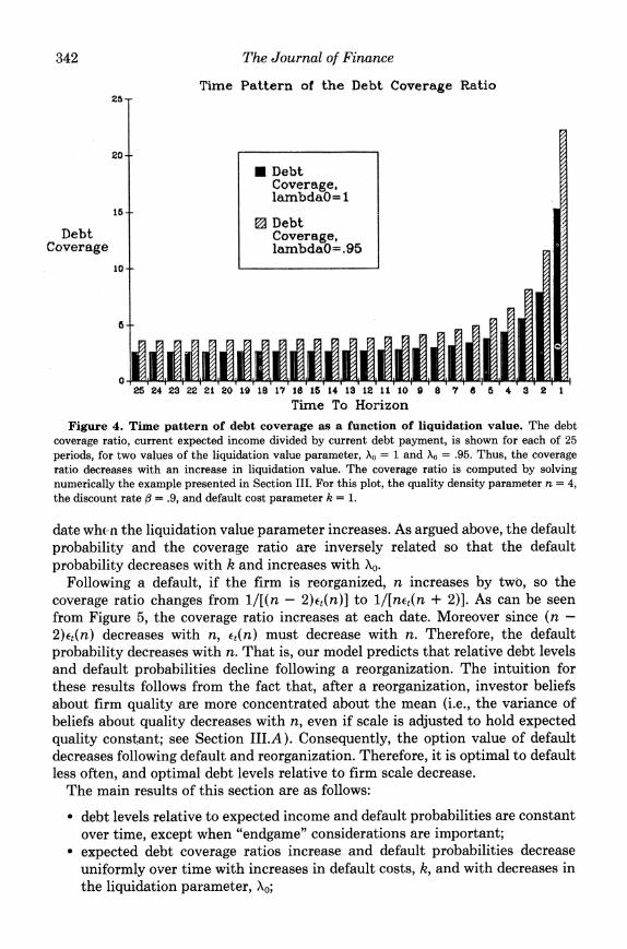
We also investigate the sensitivity of the debt coverage ratio and the default probability to changes in default costs, k, and the liquidation value parameter, Xo. In Figure 3, the coverage ratio is shown for k = .75 and k = 1. It is not surprising that, as the costs of default increase, debt levels decline relative to expected income at each date. In Figure 4, the coverage ratio is shown for Xo = .95 and Xo = 1.Since the option to liquidate is worth more when liquidation value increases, it is easy to see why, in Figure 4, relative debt levels increase at each

The Journal of Finance

Time Pattern of the Debt Coverage Ratio

Coverage,lambdaO=1i Debt

Debt Coverage

Time To Horizon Figure 4. Time pattern of debt coverage as a function of liquidation value. The debt

coverage ratio, current expected income divided by current debt payment, is shown for each of 25 periods, for two values of the liquidation value parameter, Xo = 1and XQ = .95. Thus, the coverage ratio decreases with an increase in liquidation value. The coverage ratio is computed by solving numerically the example presented in Section 111.For this plot, the quality density parameter n = 4, the discount rate p = .9, and default cost parameter k = 1.

date whc n the liquidation value parameter increases. As argued above, the default probability and the coverage ratio are inversely related so that the default probability decreases with k and increases with Xo.

Following a default, if the firm is reorganized, n increases by two, so the coverage ratio changes from l / [ (n - 2)~, (n)]to l / [n~ , (n+ 2)]. As can be seen from Figure 5, the coverage ratio increases a t each date. Moreover since ( n -2)tt(n) decreases with n, e (n ) must decrease with n. Therefore, the default probability decreases with n. That is, our model predicts that relative debt levels and default probabilities decline following a reorganization. The intuition for these results follows from the fact that, after a reorganization, investor beliefs about firm quality are more concentrated about the mean (i.e., the variance of beliefs about quality decreases with n, even if scale is adjusted to hold expected quality constant; see Section 1II.A). Consequently, the option value of default decreases following default and reorganization. Therefore, it is optimal to default less often, and optimal debt levels relative to firm scale decrease.

The main results of this section are as follows:

debt levels relative to expected income and default probabilities are constant over time, except when "endgame" considerations are important; expected debt coverage ratios increase and default probabilities decrease uniformly over time with increases in default costs, k, and with decreases in the liquidation parameter, Xo;


Time Pattern of the Debt Coverage Ratio 26

20

15

Debt Coverage

10

5

0 25 24 23 22 21 20 ID 18 17 18 15 14 13 12 11 10 9 8 7 8 5 4 9 2 1

Time To Horizon

Figure 5. Time pattern of the debt coverage ratio. The debt coverage ratio, current expected income divided by current debt payment, is shown for each of 25 periods, for two values of the quality density parameter, n = 4 and n = 6. This represents the situation before (n = 4) and after ( n= 6) a reorganization. Thus, the coverage ratio increases after a reorganization. The coverage ratio is computed by solving numerically the example presented in Section 111. For this plot, the default cost parameter k = 1,the discount rate p = .9, and the liquidation value parameter A, = 1.

expected debt coverage ratios increase and default probabilities decrease following reorganization.

The stability of coverage ratios and default probabilities over time depends strongly on our assumptions that k and At are constant over time if one is sufficiently far removed from the horizon.23 By assuming appropriate time variation of the default costs and/or liquidation value, this model is capable of generating virtually any debt repayment paths. For example, if At's are small for an initial period and then increase, the debt repayment pattern will resemble that of pure discount bonds. The dynamic implications of the model can be tested by verifying that the time patterns of observed default costs and liquidation value generate, in our model, the observed time pattern of debt levels and default probabilities.

IV. Conclusions

This paper stresses the role of debt in allowing investors to generate information useful for monitoring management and implementing efficient operating deci-sions. The significance of these benefits is highlighted by Jensen's (1989) argu-

23 At is the present value of an annuity which, for a sufficiently distant horizon, is (approximate y) independent of t.


ment that their recognition is, a t least in part, responsible for the recent increase in corporate debt levels. Trading off the value created due to these advantages against the costs of default leads to an optimal capital structure. This theory highlights the importance of liquidation value, default costs, and investor beliefs about firm quality. I t also allows predictions regarding default probabilities and the probability that a firm in financial distress will reorganize rather than liquidate.

One of the main difficulties with the model is that the complicated learning process involved makes it difficult to analyze. This difficulty is especially acute in the dynamic model, where we were forced to make specific distributional assumptions and to rely on numerical solutions for some comparative statics results. We argue, however, that the learning process is inherent in the view that informational aspects of debt are important. If a review of the firm's operating policy is contingent on income, as is the case with debt contracts, then observations of payments (or of income if it is observable) will result in revision of beliefs. Moreover, if liquidation is not automatic following default, then this decision must be based on further observations during bankruptcy. Therefore, dynamic updating of beliefs is unavoidable in any model based on this idea.

Appendix

In this Appendix, we provide formal proofs of those propositions that require them and derive the explicit solution of the dynamic model described in Section 111.

LEMMA:Given the constant returns to scale assumption, firm scale, s, is a scale parameter for the distributions H(x; s), H(x2 I XI, s), H(xz I XI, a, s), F ( a I x, s), pC(qI D, s), pd(q I x, s), and pi(q I x, a, s) (see equation (I)),and the means i ( s ) , iiC(D,s),id(x ,s),and i i (x, a, s) all exhibit constant returns to scale.

Proof: We will prove this for H(x; s) and i ( s ) . The others follow using similar arguments.

r rn

= lrnh(x I s t ) p ( t I 1)dt (using the change of variable t = q/s)

= lrn(l/s)h(x/s I t ) p ( t I 1)dt

= (11s) h(x/s; 1).

This implies that H(x; s ) = H(x/s; 1).


(x/s)h(x/s; 1)dx = th(t; 1) sdt = si(1).

Q.E.D.

Derivation of Equation (5)

First substitute for B in equation (3) from (2). This yields

However,

Therefore, substituting for ic(D, p ) [ l - H(D; p) ] in the above expression yields the objective function in (5).

Proof of Proposition 1:That P (R I x, s ) is independent of K and D is obvious. Since ii(x, a, S) is increasing in a, if L shifts up for all x, a, and s, then a(x, s ) increases for any x and s. This reduces 1- F[a(x, s ) I x, s]. If x increases but L does not, then iishifts up and L either shifts down or does not move. This results in a decrease in a(x, s) . Moreover, the increase in x shifts the distribution F ( a I x, s) down (first-order stochastic dominance). Therefore, P ( R I x, s ) increases.

Under the constant returns to scale assumption and using the previous lemma, if a(x, s ) satisfies L(x, a, s ) = p5ii(x, a, s), then a(x, s)/s satisfies L(x/s, a, 1) = pii(x/s, a, 1).Therefore, a(x, s)/s = a(x/s, 1). Consequently, using the constant returns to scale assumption and the previous lemma,

Q.E.D.

Proof of Proposition 2: We assume that the second-order condition holds; i.e., [(D, S) - K(D, s ) as a function of D cuts pid(D, S) from above a t D(s). A shift up of K or down of L shifts [ -K down but does not affect pid. Therefore, D(s) decreases if K shifts up and increases if L shifts up. Since i is independent of K and L, the expected debt coverage ratio moves in the opposite direction from D(s) . Using the lemma, it is easy to show that [ - K exhibits constant returns to scale. Therefore, D ( s ) also exhibits constant returns to scale. Q.E.D.

Proof of Proposition 3: The first statement follows immediately from Proposi- tion 2. Under the constant returns to scale assumption, H[D(s); s] = H[D(s)/s; 11= H[D(1);1] for any s. Q.E.D.

Proof of Proposition 4: From equation (4), [ shifts up with an upward shift in L. Therefore, for any given D, the objective function in (5) shifts up with an


upward shift in L. Consequently, the maximized value of this objective function, i.e., v, also increases. The proof for K is the same except for sign.

In the lemma we showed that s is a scale parameter for h(x; s) and that 2 and gd exhibit constant returns to scale. It also follows from the lemma and the constant returns to scale assumption that [ exhibits constant returns to scale. From Proposition 2, D(s) is proportional to s. Therefore, for any a # 0,

nD(s)

v(as) = (1+ P)aZ(s) + [[(x, as) - K(x, as) - PZd(x, as)] h(x; as) dx

where we have used the change of variable u = xla. Q.E.D.

Proof of Proposition 5: Let X(a, D, s) = (x I ~ ( x ,a, s) + x - K(x, s) r D > x]. It is easy to check that, under the constant returns to scale assumption, x EX(a, D, s) if and only if x/s E X(a/s, Dls, 1).Then

= 1-sPr(fu1l value) h(x; s)f(a; s ) dxda + 1 - H[D(s); s] X[a,D(s),sl

lm h(t ; l)f(u; 1)dtdu + 1- H[D(s)/s; 11. = SX[u,D(s)/s,ll

The last expression is obtained using the changes of variable t = x/s and u = a/ s and is independent of s, since D(s) is proportional to s.

Under the constant returns to scale assumption, the expected payment to bondholders is

B = D(s)Pr(full value)

= s(Pr(ful1 value) D (s)/s

[L(t, u, 1) + x - K(t, l ) ]h( t ; l)f(u; 1)dtdu],+ 1-SY[u,D(s)/s,ll

where Y(a, D, s) = (x I L(x, a, s ) + x - K(x, s) < Dl. Therefore, since D(s)/s is independent of s, we see that B is proportional to s.

Since D(s) and B are proportional to s, the promised yield, [D(s)/PB] - 1is independent of s. Also, since B and v are proportional to s, B/V is independent of s. Q.E.D.

Comparative Statics Results on Pr(Ful1 Value) and B

Given the specific functional forms described in Section 111, the critical value of the audit signal for the liquidation decision is


Substitution of a(x, s, n ) into (4) gives

where

Therefore, the first-order condition is

From (lo), the optimal debt level is given by

D(s, n) = s [ (n - l )u (n ) - P]/[P - ( n - l ) ( a (n ) - (11)k)] = ~ ( n ) s . ~ ~

The condition that debtholders receive full value is X(n)(s + x) + x(1 - k) 2

~ ( n ) s .The minimum value of X(n) required for debtholders to receive full value even when current income is zero is t (n) . If X(n) < t (n) , then debtholders receive full value if current income, x r 6(s, n) , where

Thus, the probability that debtholders receive full value is 1if h(n) r ~ ( n )and is 1-H[6(s, n); s, n] otherwise. (It can be shown that, if D(s, n) is interior, then 6(s, n) <D(s, n).) The result that Pr(ful1 value) increases in K follows from our assumption on H and our expressions for 6 and E .

Using the above results, 6

B = D[l - H(6; s , n)] + [h(n)(s+ x) + (1- k)x]h(x; s, n )

= [s/(n - 2)][(1 - k + X(n))H(G(s, n); s, n - 1)+ ( n - 2)X(n)J.

Since 1-H(6; s , n ) is increasing in k for any n, B is decreasing in default costs.

Solution of the Dynamic Model

The derivation is by induction on t. The boundary conditions are irT(n) = 1 and €T(n) = aT(n) = 0. Therefore, VT is proportional to ?(s, n) by assumption. Suppose, for some t < T - n ) = n) for some number w,+,(n) 1, V,+~(S, ~ , + ~ ( n ) ? ( s , that is independent of s and for all s and n. We claim that this implies that vt also satisfies this property for some T,. First, note that, using this expression for u t + ~and our specific distributions, we can write

&(x, S, n) = H[at(x, s, n); s + x, n + l]Xt(n)(s+ x)

24 This formula assumes an interior solution, i.e., that ~ ( n ) > 0. If X(n) <Pin, then it is optimal to continue even if a = 0 (i.e., a(x, s, n) < 0). In this case, the optimal debt level is D = 0. If u(n) - D l ( n - 1)> k, then the benefit always outweighs the cost, and the optimal debt level is infinite. In all other cases, the solution is interior.


where

and

Second, the first-order condition for D from (7 )is

[Pvt+l(s+ D, n ) - Et(D, s, n ) + k D ] h ( D ; s, n ) / [ l - H ( D ; s, n ) ]

Substituting our specific distributions for h and H and x,+,(n)Z(s + D, n ) for ~ , + ~ ( s+ D, n ) in this expression and using the above value for E,, we obtain

Solving for D gives Dt(s, n ) = ~ , ( n ) s ,where

Substitution of the optimal value of D into (7 )gives v,(s,n) = r , (n ) i ( s , n ) ,where

This shows that the solution given in Section I11 is correct.

25 This expression is correct if it is nonnegative. Otherwise, a, = D, = 0.

REFERENCES

Braden, David J. and Marshall Freimer, 1989, Newsboy distributions, Working Paper, Simon Graduate School of Management, University of Rochester.

Bulow, Jeremy I. and John B. Shoven, 1978, The bankruptcy decision, Bell Journal of Economics 9, 437-456.

Chang, Chun, 1987, Contractual Models of the Firm: A Financial Theory, Ph.D. Dissertation, Department of Finance, Kellogg School, Northwestern University.

Diamond, Douglas, 1984, Financial intermediation and delegated monitoring, Review of Economic Studies 51, 393-414.

-, 1989, Reputation acquisition in debt markets, Journal of Political Economy 97,828-862. Gale, D. and M. Hellwig, 1985, Incentive compatible debt contracts: The one period problem, Review

of Economic Studies 52, 647-663. Gertner, Robert, 1989, Inefficiency in three-person bargaining, Working Paper, Graduate School of

Business, University of Chicago. Harris, Milton, 1987, Dynamic Equilibrium Analysis (Oxford University Press, New York). -and Artur Raviv, 1988, Corporate control contests and capital structure, Journal of Financial

Economics 20,55-86. Hart, Oliver and John Moore, 1989, Default and renegotiation: A dynamic model of debt, Working

Paper, Harvard Business School. Haugen, Robert A. and Lemma W. Senbet, 1978, The insignificance of bankruptcy costs to the theory

of optimal capital structure, Journal of Finance 33, 383-393. Jensen, Michael C., 1986, Agency costs of free cash flow, corporate finance, and takeovers, American

Economic Review 76, 323-329. -, 1989, Active investors, LBOs, and the privatization of bankruptcy, Working Paper, Harvard

Business School.


-and William H. Meckling, 1976, Theory of the firm: Managerial behavior, agency costs and ownership structure, Journal of Financial Economics 3, 305-360.

John, Kose and David C. Nachman, 1985, Risky debt, investment incentives, and reputation in a sequential equilibrium, Journal of Finance 40,863-878.

Leland, Hayne and David Pyle, 1977, Informational asymmetries, financial structure, and financial intermediation, Journal of Finance 32, 371-387.

Milgrom, P., 1981, Good news and bad news: Representation theorems and applications, Bell Journal of Economics 12, 380-391.

Modigliani, Franco and Merton Miller, 1963, Corporate income taxes and the cost of capital: A correction, American Economic Review 53, 433-443.

Myers, Stewart, 1977, Determinants of corporate borrowing, Journal of Financial Economics 5, 147- 175.

Ross, Stephen A., 1977, The determination of financial structure: The incentive-signalling approach, Bell Journal of Economics 8, 23-40.

Smith, Clifford, 1986, Investment banking and the capital acquisition process, Journal of Financial Economics 15, 3-29.

Titman, Sheridan, 1984, The effect of capital structure on a firm's liquidation decision, Journal of Financial Economics 13, 137-151.

Townsend, R., 1979, Optimal contracts and competitive markets with costly state verification, Journal of Economic Theory 21, 265-293.

You have printed the following article:

Capital Structure and the Informational Role of DebtMilton Harris; Artur RavivThe Journal of Finance, Vol. 45, No. 2. (Jun., 1990), pp. 321-349.Stable URL:


This article references the following linked citations. If you are trying to access articles from anoff-campus location, you may be required to first logon via your library web site to access JSTOR. Pleasevisit your library's website or contact a librarian to learn about options for remote access to JSTOR.

[Footnotes]

7 Reputation Acquisition in Debt MarketsDouglas W. DiamondThe Journal of Political Economy, Vol. 97, No. 4. (Aug., 1989), pp. 828-862.Stable URL:

http://links.jstor.org/sici?sici=0022-3808%28198908%2997%3A4%3C828%3ARAIDM%3E2.0.CO%3B2-4

7 Risky Debt, Investment Incentives, and Reputation in a Sequential EquilibriumKose John; David C. NachmanThe Journal of Finance, Vol. 40, No. 3, Papers and Proceedings of the Forty-Third Annual MeetingAmerican Finance Association, Dallas, Texas, December 28-30, 1984. (Jul., 1985), pp. 863-878.Stable URL:

http://links.jstor.org/sici?sici=0022-1082%28198507%2940%3A3%3C863%3ARDIIAR%3E2.0.CO%3B2-H

References

Financial Intermediation and Delegated MonitoringDouglas W. DiamondThe Review of Economic Studies, Vol. 51, No. 3. (Jul., 1984), pp. 393-414.Stable URL:

http://links.jstor.org/sici?sici=0034-6527%28198407%2951%3A3%3C393%3AFIADM%3E2.0.CO%3B2-1

http://www.jstor.org

LINKED CITATIONS- Page 1 of 3 -

NOTE: The reference numbering from the original has been maintained in this citation list.

http://links.jstor.org/sici?sici=0022-1082%28199006%2945%3A2%3C321%3ACSATIR%3E2.0.CO%3B2-N&origin=JSTOR-pdf

http://links.jstor.org/sici?sici=0022-3808%28198908%2997%3A4%3C828%3ARAIDM%3E2.0.CO%3B2-4&origin=JSTOR-pdf

http://links.jstor.org/sici?sici=0022-1082%28198507%2940%3A3%3C863%3ARDIIAR%3E2.0.CO%3B2-H&origin=JSTOR-pdf

http://links.jstor.org/sici?sici=0034-6527%28198407%2951%3A3%3C393%3AFIADM%3E2.0.CO%3B2-1&origin=JSTOR-pdf

Reputation Acquisition in Debt MarketsDouglas W. DiamondThe Journal of Political Economy, Vol. 97, No. 4. (Aug., 1989), pp. 828-862.Stable URL:

http://links.jstor.org/sici?sici=0022-3808%28198908%2997%3A4%3C828%3ARAIDM%3E2.0.CO%3B2-4

Incentive-Compatible Debt Contracts: The One-Period ProblemDouglas Gale; Martin HellwigThe Review of Economic Studies, Vol. 52, No. 4. (Oct., 1985), pp. 647-663.Stable URL:

http://links.jstor.org/sici?sici=0034-6527%28198510%2952%3A4%3C647%3AIDCTOP%3E2.0.CO%3B2-W

The Insignificance of Bankruptcy Costs to the Theory of Optimal Capital StructureRobert A. Haugen; Lemma W. SenbetThe Journal of Finance, Vol. 33, No. 2. (May, 1978), pp. 383-393.Stable URL:

http://links.jstor.org/sici?sici=0022-1082%28197805%2933%3A2%3C383%3ATIOBCT%3E2.0.CO%3B2-5

Agency Costs of Free Cash Flow, Corporate Finance, and TakeoversMichael C. JensenThe American Economic Review, Vol. 76, No. 2, Papers and Proceedings of the Ninety-EighthAnnual Meeting of the American Economic Association. (May, 1986), pp. 323-329.Stable URL:

http://links.jstor.org/sici?sici=0002-8282%28198605%2976%3A2%3C323%3AACOFCF%3E2.0.CO%3B2-M

Risky Debt, Investment Incentives, and Reputation in a Sequential EquilibriumKose John; David C. NachmanThe Journal of Finance, Vol. 40, No. 3, Papers and Proceedings of the Forty-Third Annual MeetingAmerican Finance Association, Dallas, Texas, December 28-30, 1984. (Jul., 1985), pp. 863-878.Stable URL:

http://links.jstor.org/sici?sici=0022-1082%28198507%2940%3A3%3C863%3ARDIIAR%3E2.0.CO%3B2-H




http://links.jstor.org/sici?sici=0022-3808%28198908%2997%3A4%3C828%3ARAIDM%3E2.0.CO%3B2-4&origin=JSTOR-pdf

http://links.jstor.org/sici?sici=0034-6527%28198510%2952%3A4%3C647%3AIDCTOP%3E2.0.CO%3B2-W&origin=JSTOR-pdf

http://links.jstor.org/sici?sici=0022-1082%28197805%2933%3A2%3C383%3ATIOBCT%3E2.0.CO%3B2-5&origin=JSTOR-pdf

http://links.jstor.org/sici?sici=0002-8282%28198605%2976%3A2%3C323%3AACOFCF%3E2.0.CO%3B2-M&origin=JSTOR-pdf

http://links.jstor.org/sici?sici=0022-1082%28198507%2940%3A3%3C863%3ARDIIAR%3E2.0.CO%3B2-H&origin=JSTOR-pdf

Informational Asymmetries, Financial Structure, and Financial IntermediationHayne E. Leland; David H. PyleThe Journal of Finance, Vol. 32, No. 2, Papers and Proceedings of the Thirty-Fifth Annual Meetingof the American Finance Association, Atlantic City, New Jersey, September 16-18, 1976. (May,1977), pp. 371-387.Stable URL:

http://links.jstor.org/sici?sici=0022-1082%28197705%2932%3A2%3C371%3AIAFSAF%3E2.0.CO%3B2-E

Corporate Income Taxes and the Cost of Capital: A CorrectionFranco Modigliani; Merton H. MillerThe American Economic Review, Vol. 53, No. 3. (Jun., 1963), pp. 433-443.Stable URL:

http://links.jstor.org/sici?sici=0002-8282%28196306%2953%3A3%3C433%3ACITATC%3E2.0.CO%3B2-G




http://links.jstor.org/sici?sici=0022-1082%28197705%2932%3A2%3C371%3AIAFSAF%3E2.0.CO%3B2-E&origin=JSTOR-pdf

http://links.jstor.org/sici?sici=0002-8282%28196306%2953%3A3%3C433%3ACITATC%3E2.0.CO%3B2-G&origin=JSTOR-pdf

Documents

Capital Structure and the Informational Role of Debt ...ecsocman.hse.ru/data/871/126/1231/harris_raviv_-_cs_ai_1990.pdf · Capital Structure and the Informational Role of Debt Milton