Capital Requirements for Over-the-Counter Derivatives Central Counterparties

Li Lin and Jay Surti

WP/13/3

© 2013 International Monetary Fund WP/13/3

IMF Working Paper

Monetary and Capital Markets Department

Capital Requirements for Over-the-Counter Derivatives Central Counterparties1

Prepared by Li Lin and Jay Surti

Authorized for distribution by Michaela Erbenova

January 2013

Abstract

The central counterparties dominating the market for the clearing of over-the-counter interest rate and credit derivatives are globally systemic. Employing methodologies similar to the calculation of banks’ capital requirements against trading book exposures, this paper assesses the sensitivity of central counterparties’ required risk buffers, or capital requirements, to a range of model inputs. We find them to be highly sensitive to whether key model parameters are calibrated on a point-in-time versus stress-period basis, whether the risk tolerance metric adequately captures tail events, and the ability—or lack thereof—to define exposures on the basis of netting sets spanning multiple risk factors. Our results suggest that there are considerable benefits from having prudential authorities adopt a more prescriptive approach to for central counterparties’ risk buffers, in line with recent enhancements to the capital regime for banks.

JEL Classification Numbers: C53, C58, G23, G24, G28

Keywords: Central counterparties, capital, initial margin, default fund, G-14 dealers

Author’s E-Mail Addresses: li.lin@sbs.ox.ac.uk; jsurti@imf.org

1 The authors thank Aditya Narain for his support to the project. Helpful discussions with, and useful comments from Rory Cunningham, Jennifer Elliott, Michaela Erbenova, Asif Godall, Stan Ivanov, Ulrich Karl, Laura Kodres, Juri Marcucci, Bruno Momont, Kevin Sheppard, Nobu Sugimoto, Froukelien Wendt, Nicholas Vause, Philip Whitehurst, and Mark Zelmer are gratefully acknowledged. The usual disclaimer applies.

This Working Paper should not be reported as representing the views of the IMF. The views expressed in this Working Paper are those of the author(s) and do not necessarily represent those of the IMF or IMF policy. Working Papers describe research in progress by the author(s) and are published to elicit comments and to further debate.

2

Contents Page

Abstract ......................................................................................................................................2 

Glossary .....................................................................................................................................4 

I. Motivation and Overview .......................................................................................................5 

II. Systemic Importance of Global CCPs ...................................................................................7 

III. CCPs’ Risk Management Frameworks and Capital Buffers..............................................10 

IV. Methodology ......................................................................................................................14 A. Overview .................................................................................................................14 B. Simulation of CMs’ Positions .................................................................................15 C. Valuation of Cleared OTC-Derivatives ...................................................................25 D. Modeling Credit Spreads and the Term Structure ..................................................27 

V. Results .................................................................................................................................28 A. Cleared IRS and OIS ...............................................................................................28 B. Cleared CDS ............................................................................................................34 

VI. Policy Implications ............................................................................................................37 

References ................................................................................................................................45  Tables 1. Currency profile of cleared swaps and maturity profile of cleared IRS ..............................17 2. Mapping Original TtM into Maturity Buckets .....................................................................18 3. CM Outstanding Notional at Contract Level .......................................................................19 4. CM Outstanding Positions at Contract Level ......................................................................23 5. Impact of Changes in Direct Hedging on CCP Capital Requirements ................................29 6. Impact of Changing Market Conditions on CCP Risk Buffers............................................32 7. Adequacy of Buffers under Different Capital Models During Lehman Week ....................33 8. Size of CCP Risk Buffer under VaR and ES .......................................................................35 9. Impact of Changing Market Conditions on CCP Risk Buffers............................................36 10. Adequacy of Risk Buffers to Lehman-type Event .............................................................36  Figures 1. Size of the OTC-Derivatives Markets ....................................................................................7 2. Size of Selected G-SIBs’ OTC-Derivatives Exposures .........................................................8 3. The G-SIB-CCP Network ......................................................................................................9 4. CCPs in the Global Financial Network ................................................................................10 5. Representative CM Gross Notional OTC-Interest Rate Derivatives Positions ...................20 6. Comparing Simulated Asset-liability Ratios with Real Data ..............................................30 7. SwapClear IM Using Rolling Volatilities ............................................................................32 8. Five-day Close-out Gain-loss Distribution for a G-SIB CM ...............................................34 

3

9. ICE Clear Initial Margin Using Rolling Daily Returns and Volatilities ..............................37 10. Comparing Daily Returns on CDS on Two SN Obligors ..................................................42 11. Comparing Standardized Residuals on CDS on Two SN Obligors ...................................42 12. Fitting Residuals Using a Mixed Paretotail and Kernel Smoothed Interior ......................43 13. Residual Margins from Simulated (Copula) and Real (Paretotail) Data ...........................44 14. Residual Margins from Simulated and Real (Non-parametric) Data .................................44  Boxes 1. CCPs’ IM Models ................................................................................................................12 2. CCPs’ DF Models ................................................................................................................13  Appendixes I. List of CMs at SwapClear, ICE Clear Credit and ICE Clear Europe ...................................41 II. Modeling Credit Spreads .....................................................................................................42  Appendix Tables A1. Consolidated List of CMs at SwapClear ...........................................................................41 A2. List of CMs at ICE Clear ..................................................................................................41 

4

GLOSSARY

A-IRB Advanced Internal Ratings Based CCP Central Counterparty CDS Credit Default Swap CM Clearing Member CME Chicago Mercantile Exchange DF Default Fund DTCC Depository Trust and Clearing Corporation EONIA Euro Overnight Index Average ES Expected Shortfall EWMA Exponentially Weighted Moving Average FRA Forward Rate Agreement FVA Fair Value of Assets FVL Fair Value of Liabilities G14 Group of 14 Dealer Banks G-20 Group of 20 Countries GARCH Generalized Auto Regressive Conditional Heteroskedasticity GN Gross Notional G-SIB Global Systemically Important Bank ICE Inter Continental Exchange IM Initial Margin IRS Single-currency Interest Rate Swap ISDA International Swaps and Derivatives Association JtD Jump-to-Default LIBOR London Interbank Offered Rate MN Multi-name OIS Single-currency Overnight Interest Rate Swap OR Overlapping Ratio OTC-D Over-the-Counter Derivative PFE Potential Future Exposure SARON Swiss Average Rate Overnight SIB Systemically Important Bank SN Single-name SONIA Sterling Overnight Index Average TtM Time-to-Maturity VaR Value-at-Risk VM Variation Margin

5

I. MOTIVATION AND OVERVIEW

The scale of business activity in global over-the-counter derivatives (OTC-D) markets is very large. At the end of 2011, it far outstripped global banking and economic activity. Besides size, the volatility of the market value of outstanding OTC-D exposures is also significantly higher than the volatility of bank assets and economic output. Trading in the OTC-D markets is bilateral, either between dealers or between a dealer and its client. However, a very significant volume of contracts is re-traded with central clearing counterparties (CCPs) via a process called novation or clearing, wherein the CCP becomes a buyer to one counterparty and seller to the other. A majority of OTC-interest rate contracts are cleared and the percentage of OTC credit default swaps (CDS) that are cleared, while not yet comparably large, has been growing remarkably fast since the inception of the crisis. The global market structure of the provision of clearing services is monopolistic within a number of risk or product classes. Global clearing of OTC-interest rate products occurs almost exclusively through the SwapClear subsidiary of the U.K. CCP LCH.Clearnet. And, global clearing of OTC-CDS is dominated by the CCP InterContinental Exchange's (ICE) U.S. and U.K. subsidiaries, ICE Clear Credit and ICE Clear Europe. The market power of these major CCPs creates necessary conditions for them to be globally systemic financial institutions. Since the lion's share of these CCPs’ risk exposures is to the largest global banks, this also makes them especially effective shock transmitters. The post-crisis commitment of the G20 countries to mandate clearing of all standardized OTC-D trades will, in the absence of a change to the market structure of global clearing services, serve to exacerbate the global systemic importance of these CCPs. Gains from systemic risk reduction ensuing from this G20 reform initiative can only be secured, therefore, if high quality risk management practices are ensured at the major global CCPs. In this context, their pre-funded risk buffers are perhaps the most important component of the risk management framework. While the nature of CCPs’ businesses, balance-sheets and revenues are, in general, quite distinct from banks, their businesses generate the same types of financial risks. It is not surprising, therefore, that the methodologies used by major CCPs for determining their risk buffers—referred to as capital requirements in this paper—are similar to those developed by large global banks for calculating their capital charges against such risk exposures, particularly those held in their trading books. The enhancement of international prudential standards applying to internationally active banks—and their ongoing transcription into national regulation—are yet to find a parallel in the OTC-D CCP universe. While standard setting bodies have upgraded the principles for regulation and supervision of financial market infrastructures including for CCPs, the standards—particularly those applying to advanced models and techniques for calculating

6

risk buffers—are far from the level of detail and prescription that characterizes the new standards agreed by the Basel Committee on Banking Supervision (BCBS) for banks using advanced internal models to capitalize their risk exposures. Using conventional financial risk models and risk tolerance metrics, this paper conducts a range of sensitivity analyses to assess the impact of alternative model parameterizations on the size of CCPs’ required risk buffers. Our results indicate that capital requirements are very sensitive to a few key model inputs. The most important of these is the definition of the netting set used to determine a CCP’s outstanding exposures. We find that a widening of netting sets facilitated by use of model-implied correlations and bases between (the market values of) derivatives instruments that map into different risk factor classes; (e.g., maturity or currency), considerably eases capital requirements. Using instead a methodology akin to the Basel 2.5 standardized approach, wherein netting sets are defined only up to a risk factor class, results in a first-order increase in the margin and the default fund requirements. Other model inputs also exert a substantial impact. CDS contracts are characterized by discrete increases in loss experience when a default event occurs during a period of stressed markets. For CCPs clearing OTC-CDS, a departure from risk tolerance metrics that limit losses up to tail events towards metrics that limit losses in the tail can materially increase capital requirements. Calibrating returns, their volatility and market liquidity parameters on a stress period basis—similar to the stressed Value-at-Risk (VaR) capital charge against banks’ market risk exposures—significantly increases a CCP’s required margin and default fund. Capital requirements set by using VaR type metrics and based on point-in-time model inputs exhibit a high degree of procyclicality which can be mitigated by moving to stress period based parameter inputs. This has the benefit of attenuating the contagion impact on CCPs’ clearing members (CMs), and through them, also on the wider financial system. Our results suggest that there may be considerable benefits from prudential authorities adopting a more prescriptive approach that identifies acceptable risk tolerance metrics and sets a perimeter within which CCPs may calibrate key parameter inputs into their risk models. This process is already substantially further advanced for banks. Given banks’ dominant role in the market for OTC-D clearing, as the CCPs’ counterparties, there is a risk of providing them regulatory arbitrage opportunities if prudential standards for the same financial risks are different for banks and for CCPs. This concern may be brought into sharper relief going forward if BCBS’s ongoing fundamental review of banks’ trading book capitalization results in standardized supervisory approaches setting a floor for internal model based capitalization.

7

The rest of this paper is organized as follows. Section II provides the broader macro-financial stability context by outlining those characteristics of major CCPs that make them globally systemic. Section III describes CCPs’ risk management frameworks and the models they use to calculate their capital requirements. Section IV describes our approach to calculating CCPs’ risk buffers for OTC-interest rate swaps and OTC-CDS while section V describes our results. Section VI concludes with a discussion on policy implications.

II. SYSTEMIC IMPORTANCE OF GLOBAL CCPS2

We argue for considering the two CCPs that dominate the market for clearing OTC-interest rate and credit derivatives as globally systemic by assessing how they stack up against the three key characteristics of size, interconnectedness and degree of substitutability.3 In order to put this assessment in its proper context, we start by describing the relevant characteristics of the OTC-D markets. Global OTC-D markets

The volume of business activity in the OTC-D markets—aggregated across all products—stood at almost six times global banking assets and between nine-to-10 times global economic activity at end-2011. Markets for hedging and trading specific types of risks are correspondingly large also, with the smallest, credit derivatives, having outstanding gross notional amounting to more than ¼ of global banking assets (Figure 1). The market value of outstanding OTC-D contracts, while a fraction of global banking and economic activity, is substantially more volatile than either.

Figure 1. Size of the OTC-Derivatives Markets

Sources: BIS (2012) and IMF (2012).

2 This section is based on Scarlata et. al. (2012).

3 See International Monetary Fund, Bank for International Settlements and Financial Stability Board (2009).

648

504

110

7063

29

0

100

200

300

400

500

600

700

800

All OTC-D

Rates

Global banking assets

Global NGDP

FX

CDS

Gross notional positions outstanding in the OTC-derivative market, global banking assets & GDP(end-2011, in trillions of US dollars)

110

70

27

20

2.6 1.6

-25

0

25

50

75

100

125

150

Global banking assets

Global NGDP

All OTC-D

Rates

FX

CDS

Gross market values outstanding in the OTC-derivatives market, global banking assets and GDP (end-2011, in trillions of US dollars)

8

Systemically important banks’ (SIBs) are dominant players in the OTC-D markets. U.S. SIBs’ OTC-D exposures are large relative to, and in two cases, larger than their balance-sheets. Even when netting out the value of cash collateral and accounting for offsets arising from bilateral master netting agreements, the market value of these exposures constitute a significant proportion of their overall trading assets (Figure 2). And, while more dispersed, the situation is not materially different for non-U.S. SIBs.

Figure 2. Size of Selected G-SIBs’ OTC-Derivatives Exposures1/

Sources: Banks’ financial statements; Bloomberg; and authors’ calculations. Note: 1/ Barring Nomura, the banks in figure 2 were identified by the Financial Stability Board (2012) as G-SIBs, based on end-2011 data.

Systemic importance of global OTC-D CCPs

Lack of substitutability

The global CCP for OTC-interest rate derivatives, SwapClear, and the global CCPs for OTC-CDS, ICE Clear Credit and ICE Clear Europe—jointly called ICE Clear hereafter—appear, at the moment, to be too-difficult-to-substitute. Both novate close-to-100 percent of centrally cleared derivatives trades in their respective markets. If, in fact, mandatory clearing of standardized OTC-Ds comes about without a change in the existing distribution of market shares across the CCPs, then this lack of substitutability will become even more prominent. Size and volatility of the portfolio value of cleared derivatives

More than ⅓ of outstanding gross notional in the OTC-interest rates market is cleared, and hence, given its market share, the size of SwapClear’s business—whether measured by notional or market value—is very large. The volume of cleared credit derivatives is substantially smaller, albeit the rate of growth in clearing of the erstwhile nascent single-name (SN) contracts has been very impressive, with cleared gross notional outstanding doubling each year over the last three years. Moreover, the per-dollar-notional volatility in

0%

25%

50%

75%

100%

125%

150%

175%

BAML Citi GS JPM MS WF

Gross FVA-to-Total assets

Net FVA-to-trading book

(end-2011, in percentage points)

0%

25%

50%

75%

100%

125%

150%

175%

BARC BNP CA CS DB HSBC NOM RBS SOCGEN UBS

Gross FVA-to-Total Assets

Net FVA-to-Trading Book

(end-2011, in percentage points)

Major U.S. OTC-D dealers Major non-U.S. OTC-D dealers

9

market values is substantially larger for credit derivatives reflecting the embedded jump-to-default (JtD) risk. Interconnectedness

Both these CCPs, as well as the Chicago Mercantile Exchange (CME), which holds a large market share in futures and commodities derivatives clearing, are directly financially connected to the largest globally systemic banks (G-SIBs), making them particularly effective financial risk and stress transmitters (Figure 3). Through these G-SIBs, they are also connected to a much wider network of firms in the private and official sectors (Figure 4). A common set of G-SIB CMs at these CCPs ensures their exposure to common risk factors, thereby increasing their joint global systemic importance despite there being no direct financial interconnection between them at the moment.

Figure 3. The G-SIB-CCP Network

Sources: Chicago Mercantile Exchange, LCH.Clearnet and the InterContinental Exchange.

10

Figure 4. CCPs in the Global Financial Network

Note: SWF = Sovereign Wealth Fund.

III. CCPS’ RISK MANAGEMENT FRAMEWORKS AND CAPITAL BUFFERS

Given their global systemic importance, adoption of comprehensive and conservative risk management practices by the major CCPs, and ensuring this through the prudential frameworks applying to them is important for financial stability. A sound risk management framework contains a number of important elements.4 Among the most critical of these are the models CCPs use to set their pre-funded risk buffers. Their importance in the risk management framework derives in no small part from the fact that contingency arrangements providing additional layers of protection, including liquidity backstops and capital calls on CMs are susceptible to wrong-way risk; i.e., the risk that the value of such contingent arrangements falls at the same time as the financial risks that they are designed to protect against are realized.5

4 See IMF (2010) or Scarlata et. al. (2012) for overviews of the risk management frameworks. Internationally agreed principles for sound risk management by CCPs, that describe the essential elements of their risk management framework, are contained in the Committee on Payments and Settlements Systems and the International Organization of Securities Commissions (2012).

5 An exception is a liquidity backstop provided by the central bank, albeit in order to prove adequate, this may, in some circumstances, require forbearance with regard to collateral eligibility and valuation. This takes us into the realm of too-big-to-fail problems that, while important, are not directly relevant to this paper.

11

CCPs active in the OTC-D space novate traded contracts between counterparties; i.e., they become a buyer to one party and a seller to the other. In practice, where clearing is conducted on a strict principal-to-principal basis, CCPs novate contracts directly only with their CMs, typically, large internationally active banks.6 The client leg of a dealer-client trade, post-CCP novation, is assigned to the CM that is designated by the client as its clearing broker. In order to understand the basic elements of the construction of CCP risk buffers, it is essential to start with the fundamental building blocks; i.e., credit exposures, actual and potential, generated by derivatives trading and novation. Any cleared OTC-D contract generates two types of credit exposures.7 The first type of credit exposure arises from the current market value of the contract. When this moves in favor of the CCP, it acquires an exposure to the CM, and vice-versa. Industry practice and now regulation require that such exposures be fully provisioned on a daily basis. The amount of provisioning arising from a non-zero market value of the contract is called the contract’s variation margin (VM). As may be evident, VM can be posted either by the CCP or by the CM depending upon whether the market value of the contract is positive or negative for the CM. Counterparty VM is a net concept, with the total amount due from a CM being the sum of the market values to the CCP of all its contracts with that CM. The second type of credit exposure is the potential future exposure (PFE) and is covered by the initial margin (IM). The value of a contract will typically fluctuate widely over its tenor and conservative risk management entails that a CCP require CMs to provision for potential movements—normal and extreme—in the CCP’s exposure to them. Practically, this is done by calculating the maximum exposure at a given confidence level of the CCP to a CM over a fixed time horizon. The IM required of a CM is the sum of PFEs over that CM’s set of outstanding cleared contracts. As in the case of VM, full daily, or more frequent provisioning and adjustment of IM is required of all CMs on their cleared OTC-D portfolio (Box 1). Unlike VM, however, IM posting is one-sided; i.e., it is only posted by CMs to the CCP.

6 The legal relationship between the CCP, the CMs and their clients will vary across jurisdictions. Annex A details the current membership of SwapClear and ICE Clear.

7 We only aim at providing a brief and heuristic description of pre-funded risk buffers in this section. A formal introduction to these concepts can be found in Gregory (2012).

12

Box 1. CCPs’ IM Models

SwapClear’s margin model for cleared interest rate derivatives8

As its baseline model, SwapClear uses historical stress scenarios for the purpose of calibrating IM. Each day, an empirical distribution of standardized returns is generated using a look-back sampling window of 1250 (working) days. These returns are subsequently scaled by a prevailing volatility parameter estimated on the basis of a scaling approach applied to historical data. Using these inputs, a gain-loss distribution for each outstanding cleared portfolio is generated from which the worst-case loss (akin to using a 100 percent confidence level) over a five-day holding period is calculated.9 This portfolio loss then acts as the basis of the IM charged by SwapClear. ICE Clear Credit’s margin model for cleared CDS10

ICE Clear uses an IM model that combines a baseline theoretical stress scenario simulation methodology—to allocate margin against spread risk—with a number of add-ons for liquidity, concentration, bases, and JtD risk factors. The first step applies a netting set concept to outstanding cleared trades wherein proprietary model-implied index-to-SN and cross-maturity bases relationships are derived to generate a volume of outstanding net positions of each CM that is smaller than the volume implied by only netting direct offsets at the instrument level. Subsequently, a wide set of theoretical scenarios is applied to each CM’s portfolio to generate the expected shortfall (ES) calibrated at a 99 percent confidence level under a five-day close-out assumption. The ES calculation captures stressed credit spreads and stressed interest rate term structure. Separate models are then used to stress (i) the bid-offer width on each type of cleared contract (liquidity charge); (ii) provisions against adverse market reaction if significant positions need to be pushed through the market (concentration charge); (iii) index-to-SN and cross-maturity bases that may change under extreme conditions (basis risk charge); (iv) the simultaneous default of one obligor on which the CM has an outstanding CDS trade with ICE Clear (JtD charge); and (v) conditional on JtD, sensitivity to different recovery rate assumptions. The IM due from a CM is the sum of the ES and these add-on charges.

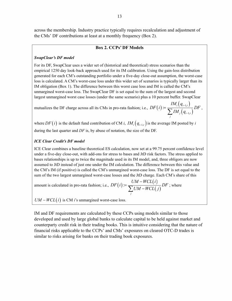
In addition to risks arising from movements in credit spreads and the term structure of interest rates, CCPs are also subject to tail risk that is not captured by the margin models. Consequently, the CCPs build a second layer of risk buffer called the default fund (DF) to pre-fund tail risk related losses. Unlike IM, wherein each CM pays 100 percent of their own contribution to potential losses to the CCP, the allocation of the DF burden is mutualized

8 This is a summary derived from LCH.Clearnet (2012a). Detailed documentation of SwapClear’s margin methodology was unavailable to the authors owing to its proprietary nature.

9 Here, a worst-case loss to the CCP is to be understood as the maximum decrease in the market value of the contract from the CM’s perspective.

10 This is a summary drawn from InterContinental Exchange (2012b, 2012c). See also InterContinental Exchange (2012a). As in the case of SwapClear, detailed documentation was unavailable owing to its proprietary nature.

13

across the membership. Industry practice typically requires recalculation and adjustment of the CMs’ DF contributions at least at a monthly frequency (Box 2).

Box 2. CCPs’ DF Models

SwapClear’s DF model

For its DF, SwapClear uses a wider set of (historical and theoretical) stress scenarios than the empirical 1250 day look-back approach used for its IM calibration. Using the gain-loss distribution generated for each CM’s outstanding portfolio under a five-day close-out assumption, the worst-case loss is calculated. A CM’s worst-case loss under this wider set of scenarios is typically larger than its IM obligation (Box 1). The difference between this worst case loss and IM is called the CM’s unmargined worst-case loss. The SwapClear DF is set equal to the sum of the largest and second largest unmargined worst case losses (under the same scenario) plus a 10 percent buffer. SwapClear

mutualizes the DF charge across all its CMs in pro-rata fashion; i.e.,

1,

1,

:i t t

j t tj

IM qDF i DF

IM q

,

where DF i is the default fund contribution of CM i, 1,i t tIM q is the average IM posted by i

during the last quarter and DF is, by abuse of notation, the size of the DF. ICE Clear Credit’s DF model

ICE Clear combines a baseline theoretical ES calculation, now set at a 99.75 percent confidence level under a five-day close-out, with add-ons for stress to bases and JtD risk factors. The stress applied to bases relationships is up to twice the magnitude used in its IM model, and, three obligors are now assumed to JtD instead of just one under the IM calculation. The difference between this value and the CM’s IM (if positive) is called the CM’s unmargined worst-case loss. The DF is set equal to the sum of the two largest unmargined worst-case losses and the JtD charge. Each CM’s share of this

amount is calculated in pro-rata fashion; i.e.,

:

j

UM WCL iDF i DF

UM WCL j

; where

UM WCL i is CM i’s unmargined worst-case loss.

IM and DF requirements are calculated by these CCPs using models similar to those developed and used by large global banks to calculate capital to be held against market and counterparty credit risk in their trading books. This is intuitive considering that the nature of financial risks applicable to the CCPs’ and CMs’ exposures on cleared OTC-D trades is similar to risks arising for banks on their trading book exposures.

14

IV. METHODOLOGY

A. Overview

As far as possible—albeit bearing in mind our information constraints as described in this and the previous section—our baseline models for IM and the DF are constructed to replicate the methodologies used by SwapClear and ICE Clear. For centrally cleared interest rate swaps (swaps)—interpreted broadly to include single currency interest rate swaps (IRS), single currency overnight index swaps (OIS) and single currency basis swaps—we estimate changes in portfolio market values using a historical volatility-scaled distribution of returns based on a 1250 day look-back period under a five-day close-out assumption. The worst-case loss for each CM pins down her IM requirement. For the DF, we start with a wider set of theoretical stress scenarios that generate more severe losses than the margin model. The DF is set equal to a Cover 2 charge; i.e., the sum of the two largest unmargined losses across all CMs, defined as the difference between the worst-case theoretical loss and the IM that they are required to post.11 For centrally cleared CDS, we use a theoretical VaR model under a five-day close out assumption to set IM, calculated as the worst-case loss at a 99 percent confidence level. We set the DF to a Cover 2 charge using a theoretical VaR model with a higher confidence level than in the IM calculation, now set at 99.75 percent. We make use of a conservative definition of the CCP’s netting set vis-à-vis each CM. As in the Basel 2.5 standardized approach—and unlike its advanced internal model based (A-IRB) approach—we do not allow for netting across risk factor classes.12 Consequently, we do not net CMs’ positions to reflect model-estimated bases or correlations between different OTC-D contracts in their cleared portfolios, nor do we, therefore, add-back basis risk. Instead, we incorporate any correlation or basis implied hedging by directly modeling the joint distribution of changes in the market value of outstanding contracts. Moreover, by calibrating key risk parameter inputs to the VaR from stressed periods for our sensitivity analyses, we are also able to address the question of how changes to bases relationships between instruments may affect capital requirements. We conduct sensitivity analyses with respect to a few key model inputs. For swaps, these include changing the degree of instrument-by-instrument hedging by CMs, using stress-period-based risk parameter inputs and assuming longer close-out periods. For CDS, these

11 A Cover k charge is one where the size of the DF is set to equal the sum of the CCP’s k largest unmargined exposures—at a chosen confidence level—across all its CMs.

12 The Basel 2.5 market risk capital rules are described BCBS (2011).

15

include changing the risk measure from VaR to ES, a tail-risk loss measure, and using stress-period-based risk parameter inputs.13 In order to calculate the risk buffers, we combine information on positions and market prices. Information on a CM’s outstanding positions at the cleared contract level is needed in order to translate the per-unit change in market value of these contracts under a given scenario into the corresponding change in market value of the CCP’s exposure to the CM. Information is also needed on prices, particularly the term structure of interest rates and credit spreads, in order to calculate the potential changes in market values of outstanding contracts over a given period of time within the remaining time to maturity (TtM). For each scenario, we calculate the per-unit-contract change in market value for all outstanding positions. We then multiply this vector of changes in market value with the vector of positions in each cleared contract. This generates a distribution of portfolio gains and losses corresponding to the set of scenarios from which we derive the worst-case loss for the CCP at a pre-fixed confidence level.

B. Simulation of CMs’ Positions

Cleared interest rate swaps In order to calculate the capital requirement, we need information on each CM’s outstanding notional long and short positions at the cleared contract level for the set of outstanding OTC interest rate derivative contracts at SwapClear at end-2011. As the information required to populate this matrix of outstanding CM positions is not available in the public domain, we simulate these positions following the approach taken by Heller and Vause (2012), albeit deviating from them along a few key dimensions. U.S. banks provide, in their regulatory filings, the sum of their long and short notional positions, aggregated separately for swaps and other types of OTC-interest rate derivatives, but not a further breakdown. Non-U.S. banks’ disclosures are coarser still, providing only the sum of their long and short positions across all types of OTC interest rate derivatives, without a further breakdown. An additional challenge is that data on positions is rarely available at the affiliate level for those G-SIBs, whose subsidiaries are themselves SwapClear CMs separately from the groups or holding companies. For example, four entities within HSBC and three within Goldman Sachs, including the groups themselves, are CMs at SwapClear. In order to operate within the constraints set by available data, we have adjusted the CM structure before proceeding with

13 ES is defined to be the expected loss conditional on losses being in excess of VaR.

16

the analysis. There are 68 CMs in all including G-SIB subsidiaries. We combine all group-affiliate CMs into one group-level CM, mindful of the fact that large global banks have strong economic incentives to have multiple affiliate companies participate simultaneously as CMs at a single CCP.14 Our consolidation reduces the number of CMs to 44. We next ask whether it is feasible to restrict attention to specific contract types. As of end-2011, 99 percent of all cleared OTC-interest rate derivatives were IRS and OIS.15 Given SwapClear’s share in this market, it is a plausible assumption that IRS and OIS also had corresponding shares of all contracts that it cleared. Consequently, for purposes of analysis, we restrict attention to IRS and OIS and assume that their shares of the total SwapClear gross notional stood at 86 percent and 14 percent respectively at end-2011. Hence, we subsume the small volume of cleared basis swaps into the cleared IRS volume. IRS In order to simulate CMs’ positions at the instrument level for cleared IRS contracts, we begin by describing the constraints implied by available information on cleared contracts at SwapClear and as reported by CM banks. We start by assembling two pieces of information provided by Trioptima for cleared contracts. First, for IRS, we have information on the distribution of contracts by remaining TtMs. Second, for all types of swaps, we have information on the distribution of cleared contracts by currency. Since over 98 percent of cleared swaps are in any one of six currencies, we restrict attention to CMs’ outstanding IRS with SwapClear in these currencies only (Table 1).

Denote a fixed, yet arbitrary IRS instrument by ; ; ;cmIRS c C m M where C is the set of

all currencies, and M is the set of all maturity buckets described in table 1. The share of

14 Large global banks, particularly those belonging to the Group of 14 dealers (G-14), typically have multiple affiliates of their group on the list of SwapClear CMs. Conversations with dealers indicate the resulting capital efficiency—owing to lower risk charges on exposures to qualifying CCPs relative to intra-group exposures under a consolidated CM model—as the primary motivation. Our institution-level, CM data on the other hand, is assembled from group-level filings—form FR-9-YC for U.S. bank holding companies, and U.S. SEC Form 20-F or annual consolidated financial statements for others. Group level notional positions already embed netting of intra-group exposures, and to this extent, the share of notional positions allocated through our assembled aggregated data to the G-14 dealers may deviate from, and understate, the real allocation. One such example that we are aware of, is of Goldman Sachs through additional data available publicly through the financial statements of its U.K. licensed subsidiary, Goldman Sachs International.

15 We obtain information on the share of each category of OTC interest rate derivatives in the total cleared notional from Trioptima whose data release for end-2011 reveals the shares of Basis Swaps, OIS, IRS and forward rate agreements (FRAs) in the global cleared notional to be three, 14, 82, and one percent respectively. The broad definition of swaps, covering the first three categories, had a share of 99 percent. The volume of cleared FRAs has increased dramatically through 2012 as reflected in the increase in their share of cleared OTC interest rate contracts from 1 percent at end 2011 to 15 percent by the end of Q3-2012.

17

cmIRS in total cleared IRS notional at SwapClear is defined as : ; cm c m where

'

'

:( )

cc

cc C

GN Swaps

GN Swaps

and

''

:( )

mm

mm M

GN IRS

GN IRS

denote, respectively, the share of the total swaps gross notional cleared in currency c, and the share of cleared IRS gross notional of remaining TtM m as of end-2011. These ratios correspond to the entries in the third and the sixth columns of table 1. Hence, the share of each IRS in our constructed SwapClear portfolio is the product of the share of interest rate swaps in the associated currency and the share of IRS of the associated remaining TtM. For example, the share of US$ IRS of less than 2 years TtM is 14¼ percent. For the A$, CHF and ¥ where the maximum TtM is 30 years, we revise the distributions accordingly.

Table 1. Currency profile of cleared swaps and maturity profile of cleared IRS (end-2011)

IRS values depend upon the fixed rate that they are contracted at; i.e., the relevant swap rate prevailing on the date when the contract was originated. Available data only gives us remaining TtM. So, we need to make assumptions regarding the distribution of the original TtM of instruments within a single maturity bucket.16 We assume that all outstanding contracts have original TtMs, (in years), from the set {2, 5, 10, 20, 30, 50}. Contracts with a given original TtM are then allocated across the reported remaining TtM buckets in symmetrically weighted fashion. For example, all 2 year original TtM US$ IRS must have a

16 Our analysis indicates that the sensitivity of portfolio value changes to alternative distributions of the original TtM of outstanding contracts is low. Nonetheless, we use different fixed rates consistent with the approach described in table 2 to increase precision. In any event, the rate at origination, i.e. the fixed rate on a contract is not a key factor affecting our results since we are not interested in portfolio value per se, but rather, in the potential change in portfolio value.

Currency Gross notional outstanding of all all swaps (in US$ billions)

Share (%)

Maturity (in years)

Gross notional outstanding of all IRS (in US$ billions)

Share (%)

US$ 90,957 36.8% 0-2 79,396 38.7%

€ 88,727 35.9% 2-5 53,395 26.0%

¥ 36,909 14.9% 5-10 48,327 23.5%

£ 24,480 9.9% 10-15 8,875 4.3%

A$ 2,886 1.2% 15-20 5,066 2.5%

CHF 2,935 1.2% 20-30 9,545 4.6%

30 & over 779 0.4%

Total 246,894 100.0% Total 205,383 100.0%

Source: Trioptima.

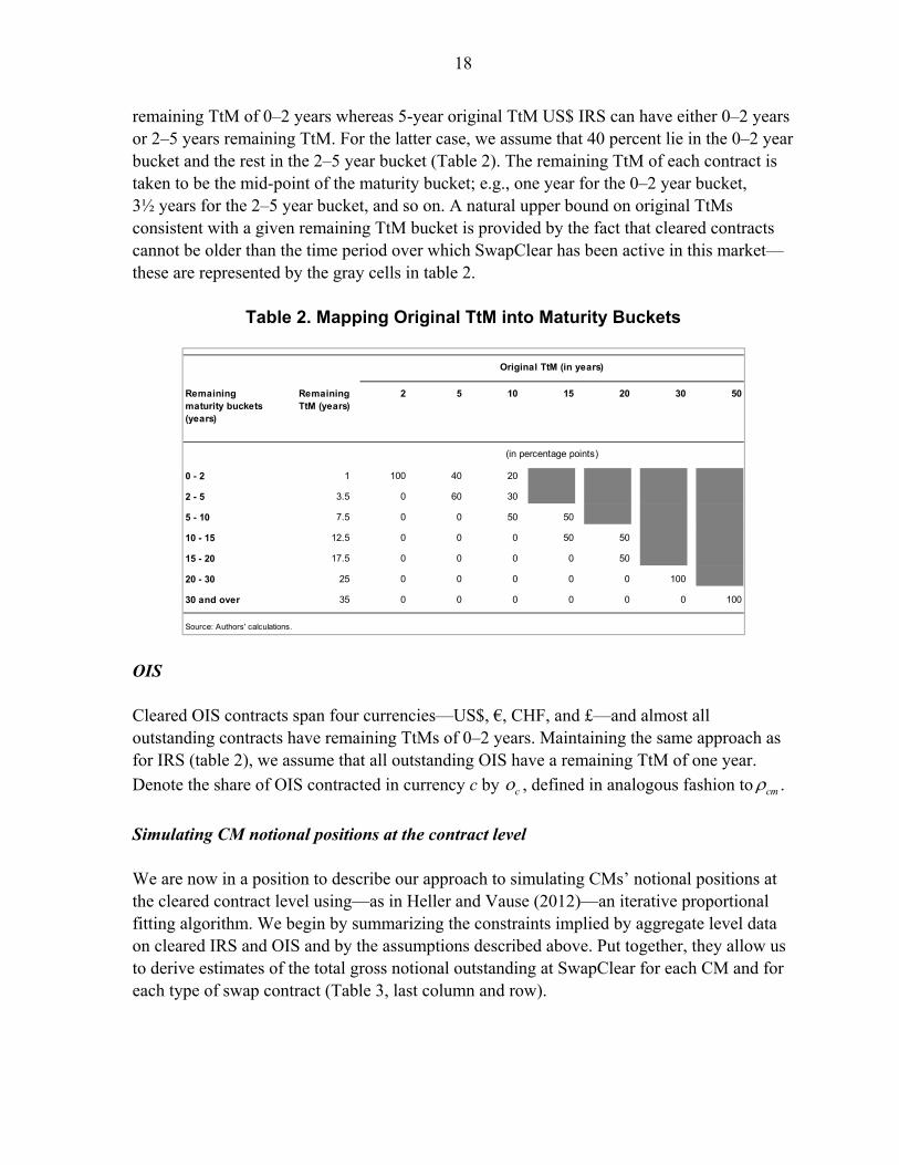
18

remaining TtM of 0–2 years whereas 5-year original TtM US$ IRS can have either 0–2 years or 2–5 years remaining TtM. For the latter case, we assume that 40 percent lie in the 0–2 year bucket and the rest in the 2–5 year bucket (Table 2). The remaining TtM of each contract is taken to be the mid-point of the maturity bucket; e.g., one year for the 0–2 year bucket, 3½ years for the 2–5 year bucket, and so on. A natural upper bound on original TtMs consistent with a given remaining TtM bucket is provided by the fact that cleared contracts cannot be older than the time period over which SwapClear has been active in this market—these are represented by the gray cells in table 2.

Table 2. Mapping Original TtM into Maturity Buckets

OIS Cleared OIS contracts span four currencies—US$, €, CHF, and £—and almost all outstanding contracts have remaining TtMs of 0–2 years. Maintaining the same approach as for IRS (table 2), we assume that all outstanding OIS have a remaining TtM of one year.

Denote the share of OIS contracted in currency c by c , defined in analogous fashion to cm .

Simulating CM notional positions at the contract level We are now in a position to describe our approach to simulating CMs’ notional positions at the cleared contract level using—as in Heller and Vause (2012)—an iterative proportional fitting algorithm. We begin by summarizing the constraints implied by aggregate level data on cleared IRS and OIS and by the assumptions described above. Put together, they allow us to derive estimates of the total gross notional outstanding at SwapClear for each CM and for each type of swap contract (Table 3, last column and row).

Remaining maturity buckets (years)

Remaining TtM (years)

2 5 10 15 20 30 50

0 - 2 1 100 40 20

2 - 5 3.5 0 60 30

5 - 10 7.5 0 0 50 50

10 - 15 12.5 0 0 0 50 50

15 - 20 17.5 0 0 0 0 50

20 - 30 25 0 0 0 0 0 100

30 and over 35 0 0 0 0 0 0 100

Source: Authors' calculations.

Original TtM (in years)

(in percentage points)

19

Table 3. CM Outstanding Notional at Contract Level

The starting point is the total gross notional volume of OTC interest rate derivatives cleared by SwapClear as of December 31, 2011, which, from LCH.Clearnet’s 2011 annual report amounted to US$ 283.4 trillion. The total gross notional outstanding of individual IRS contracts is derived by distributing the share of IRS contracts—86 percent of the total SwapClear gross notional—according to the

ratios cm derived above. Similarly, for individual OIS contracts, we distribute their share;

i.e., 14 percent of the SwapClear gross notional according to ;co c C , completing the

bottom row of table 3. Turning to the CMs’ gross notional positions, consider first, the 34 CMs that report their interest rate swaps notional. For these dealers, the share of this amount outstanding at SwapClear is estimated in two steps. First, we divide their total reported IRS and OIS notional by 99 percent, reflecting the share of these contracts in total global cleared notional (footnote 15). Second, we allocate 85 percent of this adjusted swaps notional to positions outstanding at SwapClear. This reflects the fact that CMs do not clear all of their eligible products (Figure 5).17

17 The International Swaps and Derivatives Association, in a market overview, available at http://www.isdacdsmarketplace.com/market_overview/central_clearing, indicated that major swaps dealers are committed to clearing up to 90% of their clearing eligible interest rate derivatives and were doing so as of January 2012. Nonetheless, applying this ratio to a dealer’s reported swaps notional may overstate that dealer’s positions at SwapClear since some IRS products are not clearing eligible. Balancing this to a degree is the fact that the gross notional reported in the banking group’s financial statement may underestimate the total contracts outstanding across all group affiliates that are CMs at the CCP (see footnote 14). We have chosen a clearing ratio of 85 percent bearing in mind these considerations and also because it generates a reasonable set of remaining positions for the other 10 CMs who do not report the data.

IRS1 IRS2 …. OIS1 … OIS4 Total CM position at SwapClear

CM1 GN1 (= GNL1 + GNS1)

CM2 GN2 (= GNL2 + GNS2)

… ….

SwapClear Total

86%*SC total * ρcm1 86%*SC total * ρcm2 … 14%*SC total * o 1 …. 14%*SC total * o 4 SC total

Sources: CM regulatory f ilings and f inancial statements, Derivatives Trust and Clearing Corporation (DTCC), Sw apClear, Trioptima, and authors' calculations.

(in US$ billions)

20

Figure 5. Representative CM Gross Notional OTC-Interest Rate Derivatives Positions

Sources: CMs’ regulatory filings and financial statements.

For CMs that report OTC interest rate derivatives positions but do not break these down further into swaps and other contracts, we assume that 78 percent—the same as their share in the total OTC interest rates trading notional in the global market—are in IRS and OIS. Following this, we adopt the same two-step procedure described above to calculate the notional outstanding at SwapClear. Finally, for the CMs that do not report their OTC interest rate derivatives positions, we allocate equal shares of the remaining amount of total SwapClear gross notional, completing the right column of table 3. Our interest is in estimating the missing information represented by the gray cells of table 3. Filling in the last column and row of this table assists us in obtaining 117 constraints—corresponding to 44 CMs and 73 IRS and OIS contracts—on otherwise randomly drawn granular positions. These constraints can be represented succinctly by the following two equations:

; , ; SCijh ijh ih

j

i D h H IRS OIS L S GN ; (1)

where ijhL and ijhS are long and short positions (or receive-fixed and receive-float) positions

respectively, SCihGN is CM i’s gross notional outstanding across all contracts of a specific

class h in SwapClear, and D is the set of CMs.

; ; h SCijh ijh jh

i i

j N h H L S GN ; (2)

where SCjhGN is the gross notional outstanding in an instrument in SwapClear and Nh is the

set of contract types within a specific class of contracts; i.e., IRS or OIS. In addition, we make the assumption that the shares of IRS and OIS in any CM’s portfolio of outstanding positions is the same as the share of these contracts in the CCP’s portfolio of

0

5,000

10,000

15,000

20,000

25,000

30,000

35,000

40,000

45,000

DB RBS BNP BAML JPM MS UBS CS CITI GS

(in US$ billions)

21

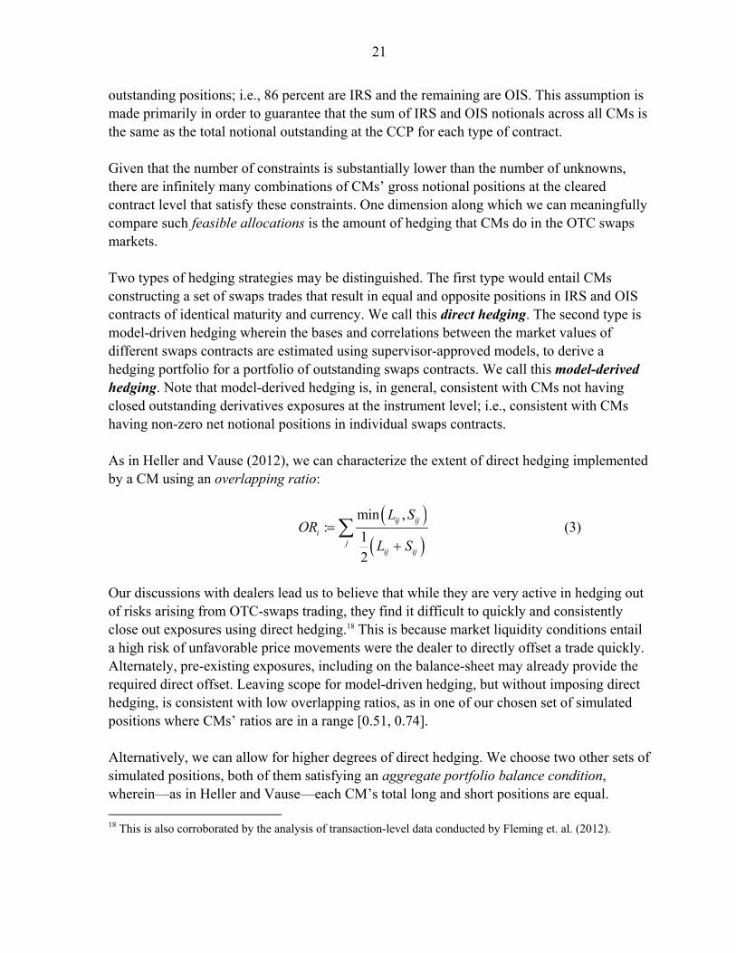
outstanding positions; i.e., 86 percent are IRS and the remaining are OIS. This assumption is made primarily in order to guarantee that the sum of IRS and OIS notionals across all CMs is the same as the total notional outstanding at the CCP for each type of contract. Given that the number of constraints is substantially lower than the number of unknowns, there are infinitely many combinations of CMs’ gross notional positions at the cleared contract level that satisfy these constraints. One dimension along which we can meaningfully compare such feasible allocations is the amount of hedging that CMs do in the OTC swaps markets. Two types of hedging strategies may be distinguished. The first type would entail CMs constructing a set of swaps trades that result in equal and opposite positions in IRS and OIS contracts of identical maturity and currency. We call this direct hedging. The second type is model-driven hedging wherein the bases and correlations between the market values of different swaps contracts are estimated using supervisor-approved models, to derive a hedging portfolio for a portfolio of outstanding swaps contracts. We call this model-derived hedging. Note that model-derived hedging is, in general, consistent with CMs not having closed outstanding derivatives exposures at the instrument level; i.e., consistent with CMs having non-zero net notional positions in individual swaps contracts. As in Heller and Vause (2012), we can characterize the extent of direct hedging implemented by a CM using an overlapping ratio:

min ,

:1

2

ij ij

ij

ij ij

L SOR

L S

(3)

Our discussions with dealers lead us to believe that while they are very active in hedging out of risks arising from OTC-swaps trading, they find it difficult to quickly and consistently close out exposures using direct hedging.18 This is because market liquidity conditions entail a high risk of unfavorable price movements were the dealer to directly offset a trade quickly. Alternately, pre-existing exposures, including on the balance-sheet may already provide the required direct offset. Leaving scope for model-driven hedging, but without imposing direct hedging, is consistent with low overlapping ratios, as in one of our chosen set of simulated positions where CMs’ ratios are in a range [0.51, 0.74]. Alternatively, we can allow for higher degrees of direct hedging. We choose two other sets of simulated positions, both of them satisfying an aggregate portfolio balance condition, wherein—as in Heller and Vause—each CM’s total long and short positions are equal. 18 This is also corroborated by the analysis of transaction-level data conducted by Fleming et. al. (2012).

22

ijh ijhj j

L S (4)

Heller and Vause also introduce, in addition to (4), a stronger assumption directly on the values and range of CMs’ overlapping ratios generating high levels of direct hedging.19 One set of simulated positions, that both satisfies (4) and generates fair values of CMs’ interest rate swaps assets and liabilities matching end-2011 reported data, results in overlapping ratios being in a range [0.84, 0.93]. If, in addition, we introduce the stronger assumption of high levels of direct hedging, then one set of positions that generates capital requirements close to actual levels at end-2011 implies CM overlapping ratios in a range [0.99, 0.996]. Before closing this part of the discussion, it is worth noting that while we do not have an adequate set of stylized facts relating to dealers’ net positions and trading or hedging in these markets, what evidence we do possess suggests that overlapping ratios are not very high. Some of the CMs are banks with a large loan book where they receive fixed payments but where they either pay floating rates or have liabilities of a shorter duration. Consequently, one may expect such banks to take larger positions on receive-float/pay-fixed interest rate swaps, as the FFIEC-031 filings of large U.S. banks appear to suggest. On the other hand, Begeneau, Piazzesi and Schneider (2012), taking a portfolio replication approach to estimating banks’ exposures to interest rate risk emanating from activity in the interest rate derivatives market, found banks mostly taking pay-float positions. In an earlier study, Gorton and Rosen (1995) concluded that banks had large net positions that were highly sensitive to interest rate risk. Cleared CDS positions The methodology for arriving at CMs’ outstanding notional positions in cleared CDS contracts is similar to that described for CMs’ simulated positions at SwapClear. As in the previous subsection, data on contract level positions is not available for cleared CDS at ICE Clear. So, we must simulate CMs’ positions. We begin again by describing how available information guides and constrains our simulation (Table 4). Combining the business of its subsidiaries—one each in the U.S. and Europe—ICE Clear has 15 CMs and clears 221 CDS contracts referencing multi-name (MN) and SN obligors. ICE Clear reports both gross and net notional positions cleared on each of these contracts. We want to simulate the gross notional protection bought and sold by a CM for each CDS cleared by ICE Clear; i.e., the gray cells in table 4.

19 They assume that the CMs’ overlapping ratios—called similarity metrics in their paper—lie within a range (0.95, 0.99) with the average value constrained to be no more than 0.001 away from 0.98.

23

Table 4. CM Outstanding Positions at Contract Level

Let us first consider the constraints implied by information on CM positions. Barring three CMs that only report the sum of gross CDS protection bought and sold, the others report both types of positions separately. The CDS notional reported by CMs include contracts that are not eligible for clearing at ICE Clear, those that are eligible, yet not cleared and those that are both eligible and cleared. From the Depository Trust and Clearing Corporation’s (DTCC) CDS data repository, we obtain the total gross notional on all CDS contracts outstanding at ICE Clear as of end-2011. From this, we calculate the share of clearing eligible CDS in the universe of all OTC-CDS contracts. Noting that only a fraction of eligible contracts are cleared, we assume—as in the case of interest rate swaps clearing—that 85 percent of such CDS are actually cleared at ICE Clear. A CM’s gross notional protection (bought/sold) at ICE Clear as of end-2011 is 85 percent of the product of its reported CDS gross notional protection (bought/sold) and the share of clearing eligible CDS contracts.20 This completes the right column of table 4. The second set of constraints arises from estimating the gross/net notional amounts outstanding for each cleared CDS contract at ICE Clear. Without going into the details—since they are the same as for interest rate swaps cleared by SwapClear—these amounts are estimated by assuming that the distribution of total gross notional across cleared CDS on ICE

Clear is the same as in the wider DTCC universe. Hence, '

'

:jG

j

jj J

GN CDS

GN CDS

, is defined

to be the share of outstanding gross notional of the jth CDS contract cleared at ICE Clear as of end-2011. We can define an analogous concept for the distribution of net notional across

20 For the three CMs that did not report gross protection bought and sold separately, we use the fact that, by definition, the total GN protection bought on ICE Clear has to be the same as the total GN protection sold. Therefore, once we have calculated the bought and sold gross positions for the 12 CMs that report both sides, we derive a net bought position that we allocated to these three remaining CMs in proportion to their gross notional outstanding.

CDS1 CDS2 …. CM gross notional bought/sold

CM1 CM1 company filing

CM2 CM2 company filing

…. ….

ICE gross notional ICE total gross notional * ς1 ICE total gross notional * ς2

….

ICE total gross notional

ICE net notional Available from ICE Clear Available from ICE Clear …. ICE total net notional

Sources: CM regulatory f ilings and f inancial reports, DTCC, ICE Clear and authors' calculations.

(in US$ billions)

24

cleared CDS contracts. In defining these ratios, the gross notional is defined on all outstanding trades, both cleared and uncleared as reported in the DTCC repository. This completes the bottom row of table 4. These two steps set up 469 constraints on otherwise randomly generated CM gross and net notional on individual cleared CDS contracts at ICE as of end-2011. First, the sum of protections bought/sold across instruments by each CM equals her total bought/sold notional amount outstanding in the ICE portfolio.

; ICE ICEij iB ij iS

j j

i D B GN S GN

; (5)

where ICEiBGN and ICE

iSGN are CM i’s gross notional bought and sold positions in ICE.

Second, the sum of positions across dealers on each derivative must equal to the total amount of that derivative in the ICE portfolio.

; ICEij ij j

i i

j N B S GN ; (6)

where ICEjGN is the gross notional amount of derivative j in ICE Clear.

The open interest of each instrument matches the data, which is reported by ICE.

; max ,0ij ij ji

j N B S OI ; (7)

where jOI is the open interest of instrument j in ICE. The open interest of an instrument is

the sum of the net notional protections bought or sold. While the number of constraints is more than thrice that for the case of interest rate swaps, the number of unknowns is significantly larger still. As a result, there are an infinite number of combinations of CMs’ gross and net notional CDS positions that are consistent with (5)–(7). As in the case of interest rate swaps, further restrictions do not appear to arise from plausible assumptions regarding the hedging strategies of CMs. Conversations with dealers revealed that while model-driven hedging is actively pursued, direct hedging is not, as the latter is subject to the same types of implementation costs and difficulties as those described for interest rate swaps. Indeed, as Chen et. al. (2011) also document, costs to direct hedging appear to be even higher in the CDS market than in the IRS market. Consequently, we choose a set of simulations providing for a wide range of overlapping ratios of [0.62, 0.87].21 21 Eight of the 15 CMs have an overlapping ratio of greater than 80 percent and only two have an overlapping ratio of less than 70 percent. Heller and Vause constrain this ratio to lie in a range [0.8, 0.94] with the average value being no more than 0.001 away from 0.89.

25

C. Valuation of Cleared OTC-Derivatives

IRS The mark-to-market value of an IRS contract is the difference between the present value of the receive-fixed and pay-float legs.

1

1

1

1 ,

1

n tn

n tn

n n

receive fixed leg pay float legj j j

Nt rreceive fixed leg

j n n jn

Nt rpay float leg f

j n n t tn

MV PV PV

PV e t t r

PV e t t r

where n tnt r

e

is the discount factor withnt

r being the LIBOR discount rate; jr , the fixed rate on

the contract; 1 ,n n

ft tr

, the forward rate between two payment dates 1and n nt t ; and N, the

number of payments. We assume a quarterly payment frequency. OIS The mark to market value of an OIS contract is also the difference between the present value of the receive-fixed and pay-float legs. The fixed rate is predetermined while the floating rate is the geometric average of the overnight rates starting from the last payment date to the next one. Therefore the present value of the pay-floating leg is adjusted as

1

/1

1

1 1365

nn tn

n

o ntNt rpay float leg s

jn s t

rPV e

for OIS-£ contracts. For the other three currencies, the corresponding expression is

1

/1

1

1 1360

nn tn

n

o ntNt rpay float leg s

jn s t

rPV e

The geometric average of the overnight rate is bootstrapped from the OIS curve. Since we assume all contracts have one year remaining TtM and that the payment is made once per year, valuing the OIS contract at today is straightforward. The expected geometric average of the overnight rate from today to maturity equals to the fixed rate on the traded OIS contract with one year TtM. To value the OIS contract k days later is slightly more involved. The overnight rate in the following k–1 days will have been realized at day k with the remaining rates through the TtM still unknown. Therefore, we simulate the overnight rate for the

26

following k–1 days. And we obtain the geometric average of the remaining overnight rates (i.e. from day k to maturity) from the prevailing OIS curve k days away in the future. CDS The mark-to-market value of a CDS contract (consider per notional amount) is the difference between the present value of the contracted premium payment and present value of the protection leg. Specifically,

premium leg protection leg

j j j

premium legj j j

MV PV PV

PV S PVBP

where jS is the contracted spread and jPVBP is the present value of the future cash flows from

a basis point of payment. The latter quantity is defined by:

1

n t n jn

Nt r t

jn

PVBP e e

;

where nt is the time from the valuation date to the thn payment date. We assume a quarterly

payment frequency. For a contract with M years remaining TtM, the total number of

payments is N = 4M; n tnt r

e

is the discount factor, withnt

r being the LIBOR discount rate;

n jte is the survival probability; and j the default density. If the underlying reference

obligor survives on the nth payment date, the buyer will continue to make the payment. The current default density is bootstrapped from the traded contract with the same underlying reference obligor by setting the present value of the premium leg equal to the present value of the protection leg of that traded contract:

' '

1' ' '

1 1

1n t n tn j n j n jn n

N Nt r t rt t tpremium leg protection leg

n n

S e e PV PV e e e R

;

where 'S is the spread for a traded CDS with the same underlying; 'N , the corresponding payment numbers; and R, the recovery rate. With a group of traded CDS on the same underlying reference obligor but of different maturity, one could bootstrap a term structure of the default density.22 Note that since the default density is bootstrapped from market data, it is a risk-neutral measure.

22 In this paper we consider traded CDS of 5 year maturity and therefore the default density is constant. For detailed discussions on the valuation of CDS contracts, see Duffie and Singleton (2003) and O'Kane and Turnbull (2003).

27

Finally, the present value of the protection leg of the contract we want to value is given by:

1

1

1n t n j n jn

Nt r t tprotection leg

jn

PV e e e R

D. Modeling Credit Spreads and the Term Structure

To forecast the future market value of OTC-derivatives, we simulate market data relevant for the purposes of valuation. The time series include all interest rates relevant for establishing the LIBOR discount curves. The rates include short-term LIBOR rates with maturity of less than 6 months, interest rate futures between 6 months and 4 years and IRS rates with maturities from one year to 50 years. The types and number of rates included vary across different currencies depending on data availability. For valuing OIS contracts, we include the relevant overnight rates (the U.S. Federal Funds rate, the EONIA, the SONIA, and the SARON). Finally, for valuation of CDS contracts, we add the time series on the premia on all SN and MN CDS contracts with five-years remaining TtM. Two types of models are used to simulate the distribution of changes in market value of the derivatives portfolio. First, following SwapClear, we use historical stress scenarios for the purpose of calculating IM.23 A look-back period of 1250 days is adopted and the rolling five-day or 10-day standardized return on the sample is calculated. Then, these standardized returns are scaled by the prevailing volatility at the chosen valuation date. The prevailing volatility is estimated using an exponentially weighted moving average (EWMA) approach. Second, we model theoretical stress scenarios, wherein we fit each time series into an asymmetric GARCH model to capture the volatility clustering feature of time series and allow the conditional variance to respond differently to past negative and positive innovations.24

1

1

2 2 221 1 1 0t

t t t

t t t t e

t t t

r r e

e e I

e z

where tr is the daily log return at date t, t the conditional volatility of tr , tz is the

standardized residual, and 1teI

is given the usual definition of a characteristic function that

takes the value one if the subscript is negative and zero otherwise. The standardized residuals

23 An introduction to historical simulation can be found in Hull and While (1998).

24 Except for the overnight rates of the US$ and the A$ for which daily returns are zero for a majority of the time.

28

from the GARCH model are fitted using a non-parametric distribution (Annex B). Since we are interested in the joint movements of the time series, the joint distributions of the residuals are then fitted with a copula. We use the estimated copula to generate random distributions of the residuals which are then introduced into the estimated GARCH model to simulate data.

V. RESULTS

A. Cleared IRS and OIS

At end-2011, SwapClear had total IM amounting to US$ 17.2 billion and a DF of US$ 206 million. Subsequent developments have resulted in an increase in the DF to US$ 4 billion by October 2012. This reflects changes to SwapClear’s risk management framework as it pertains to its default management process. These included, prominently, the creation of a segregated SwapClear DF with a size floor of £ 1 billion; inclusion of the SwapClear default management process within the LCH.Clearnet rulebook, instead of being set out as a private agreement; and, dropping requirements relating to minimum portfolio size, own-capital and credit rating for a financial institution to become a SwapClear CM.25 These changes resulted in an increase in assessed DF contributions, including a five-fold increase in the CMs’ minimum contributions, from £ 2 million to £ 10 million. Capital requirements are highly sensitive to the amount of direct hedging by CMs As discussed in the previous section, there are infinitely many combinations of CMs’ (simulated) cleared swaps positions that would satisfy the basic constraints implied by the data; i.e., (1) and (2). Of these, infinitely many survive when we impose an aggregate portfolio balance requirement; i.e., (4). Subsequently, we chose 3 sets of positions, distinguished by the amount of direct hedging that CMs are able to implement. The first set of simulated positions—Positions 1—is one characterized by a very high level of direct hedging where CMs directly offset between 99-to-99½ percent of cleared exposures through opposite positions taken at SwapClear. In fact, Positions 1 was reverse engineered to obtain IM and DF requirements sufficiently close to their actual levels (Table 5). We interpret this result to give us the amount of direct hedging CMs must implement in order to render these levels of risk buffer adequate relative to the specified risk tolerance level.

25 LCH.Clearnet (2012b) provides further details.

29

Table 5. Impact of Changes in Direct Hedging on CCP Capital Requirements

In contrast, when we imposed only the aggregate portfolio balance requirement (4), the chosen simulation—Positions 2—exhibited overlapping ratios in a lower range of values, from the set [0.84, 0.93]. Lower levels of direct hedging exert a substantial impact, raising the required IM to US$ 169 billion and the required DF to US$ 89 billion. If we also relax (4), the simulated Positions 3 exhibit still lower overlapping ratios resulting in further increases of 267 percent in the IM and 460 percent in the DF. One approach to validating the simulated Positions 1, 2 and 3, is to compare their ranges of the ratios of CMs’ swaps assets to swaps liabilities to the ranges of these ratios, when derived from end-2011 data; i.e., [0.92, 1.09]. The range of these ratios for the chosen simulated positions is too narrow for Positions 1 and too wide for Positions 3, but approximates the real data well for Positions 2 (Table 5, Figure 6). Under this validation metric, Positions 2 appear to be the most appropriate candidate, in which case, one could ask why the capital buffers held at SwapClear are not higher.26 Our knowledge is constrained by the extent of SwapClear’s disclosures regarding its IM methodology which is unavailable in the public domain. Nonetheless, we can conjecture that

26 The real FVA/FVL ratios for CMs’ swaps portfolios are those derived for the aggregate outstanding portfolio of cleared and uncleared trades rather than for cleared volumes alone. However, it is the latter that are relevant to assessing the validity of Positions 1, 2 and 3. If the FVA/FVL ratios for cleared portfolios deviate substantially from those for the aggregate portfolio, the case for using this validation metric is weaker.

SwapClear's actual risk buffers & CMs' actual A-L ratios

Positions 1 Positions 2 Positions 3

Initial Margin 17.2 17.5 168.8 619.5

Default Fund 4.0 9.2 89.4 499.0

Overlapping ratio (range) [0.99.0.996] [0.84, 0.93] [0.51, 0.74]

Asset-Liability ratio (range) 1/ [0.92, 1.09] [0.99, 1.00] [0.87, 1.10] [0.64, 1.48]

Sources: CM f ilings and f inancial reports, LCH.Clearnet and authors' calculations.

Note:

1/ The range of CMs' fair value of assets-to-fair value of liabilities; from actual position data in the f irst column and implied by simulations of positions

1, 2 and 3. The actual A-L ratios of 5 small CMs (in the first column) w ere outside of the specif ied range.

(as of end-2011; in US$ billions, unless stated otherwise)

30

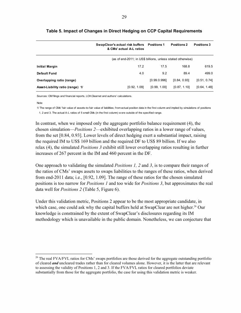
their model may include a first stage wherein the netting of CMs’ positions reflects model-derived offsets generated through bases and correlations between different cleared swaps contracts. IM is subsequently calculated at a second stage for these model-derived net positions. Equivalently, the netting sets implied by the CCP’s internal risk model are wider than in our model, and hence, their capital requirements correspondingly lower.27

Figure 6. Comparing Simulated Asset-liability Ratios with Real Data

Sources: CM filings and financial reports; and authors’ calculations. Notes:

1/ ∆ = ratio of fair value of swaps assets-to-fair value of swaps liabilities of SwapClear CMs; 2/ * = ratio of fair value of simulated swaps assets-to-fair value of simulated swaps liabilities.

27 This is akin to differences—under Basel 2.5—between an A-IRB bank’s market risk capital requirements derived under its internal model based approach and under the standardized approach.

31

Capital requirements are highly sensitive to market conditions used to calibrate key risk parameter inputs Changing market conditions may be expected to result in different levels of CCP exposures to CMs. Daily market price movements may be substantially wider during times of stress and replacing or liquidating outstanding contracts with a defaulting CM, including liquidation of collateral, may take longer and be costlier than otherwise. Capital requirements are highly sensitive to different levels of market stress assumed when calibrating risk model inputs related to the volatility of swaps market values and the length of the close-out period (Table 6). Three types of market stress levels are considered. Normal market conditions—in line with existing industry practice—we use the

standardized return over the last five working days of 2011 and the end-2011 volatility level as inputs while assuming a five-day close-out.

Volatile market conditions correspond to a setting where the volatility input is recalibrated to the higher market stress level prevailing on September 16, 2008; i.e., the Lehman Brothers default.

Illiquid market conditions correspond to a setting where it takes double the normal time; i.e., 10 days to close-out positions of defaulting CMs.

For simulated Positions 1, calibrating model inputs on the basis of volatile or illiquid market conditions results, respectively, in 22 percent and 11½ percent increases in IM requirements. It also results in increases of over 400 percent and 300 percent in the size of the required DF. For simulated Positions 2 and Positions 3, the concomitant increases are comparable or larger still. It is noteworthy that the Basel Committee on Banking Supervision, in its 2009 overhaul of banks’ market risk capital requirements, has added a stress-VaR capital charge for A-IRB banks in order to account for the perceived, high sensitivity of model-implied capital requirements to the choice of these input parameters.28

28 See the Basel Committee on Banking Supervision (2011). Using stressed market condition calibrated model inputs assists us in incorporating potential violations of normal bases/correlations in cleared CDS market values. Using longer close-out periods assists in incorporation of heightened liquidity and concentration risk.

32

Table 6. Impact of Changing Market Conditions on CCP Risk Buffers

Procyclicality of the IM Given our EWMA methodology to calibrate the prevailing volatility parameter input, daily IM resets may be expected to result in large and discrete increases in CM obligations during a sudden transition into a period of considerably higher market stress. One such transition occurred around the Lehman Brothers default event in the third quarter of 2008. Assuming that CMs’ positions are given by simulated Positions 1 and standardized returns calculated under the assumption of normal market conditions (Table 6), we calculate how the total IM requirement would evolve with the volatility input between 2007Q1 and 2010Q4. The jump in volatility in 2008 Q3 over the previous quarter results in a four-fold increase in IM requirements, from US$ 8½ billion to over US$ 33¾ billion in 2008Q3 (Figure 7).

Figure 7. SwapClear IM Using Rolling Volatilities

Source: Authors’ calculations.

Market conditions

Positions 1 Positions 2 Positions 3 Positions 1 Positions 2 Positions 3

Normal 17.5 168.8 619.5 9.2 89.4 499.0

Volatile 21.5 208.0 870.7 55.6 537.5 2,650.9

Illiquid 19.4 187.2 750.6 47.1 468.7 2,484.9

Source: Authors' calculations.

Initial Margin Default Fund

(in US$ billions)

5

15

25

35

2007Q1 2007Q2 2007Q3 2007Q4 2008Q1 2008Q2 2008Q3 2008Q4 2009Q1 2009Q2 2009Q3 2009Q4 2010Q1 2010Q2 2010Q3 2010Q4

(in U.S.$ billions)

8.6

33.7

10.6

33

Discrete jumps in margin calls by CCPs during times of extreme stress will exert an adverse knock-on effect on market volatility. SwapClear’s model currently captures a period of extreme stress in its current 1250 day look-back sampling window and this attenuates procyclicality, but this problem would reappear during periods of prolonged moderation in the future. Robustness of capital buffers to stress—the Lehman default week Finally, we look at how different modeling assumptions would impact the adequacy of resulting risk buffers if extreme market value changes of the magnitude seen during the Lehman default week are realized. We assume that simulated positions are given by Positions 1 and standardized returns are as of September 10, 2008. In setting the CMs’ IM requirements, we assume three alternative market conditions and corresponding volatility and close-out period inputs. Under normal market conditions, we assume volatility parameters as of September 10, 2008 and a five-day close-out. Under volatile markets, we assume volatility as of September 16, 2008 and a five-day close-out. And, under illiquid markets, volatility as of September 10, 2008 and a 10-day close-out. We then calculate the change in the market values of CMs’ positions between September 10 and September 17, 2008 using market data on these two days. These valuation changes are compared to the IMs for the three sets of market conditions assumed (Table 7).

Table 7. Adequacy of Buffers under Different Capital Models During Lehman Week

While unmargined losses arise for some CMs under both normal and volatile market conditions, the IM required when assuming stressed/downturn volatility is sufficiently higher

Clearing members Change in value of CM's SwapClear notional

Initial Margin Unmargined loss? Initial Margin Unmargined loss? Initial Margin Unmargined loss?

CM 1 (9,601) 63,060 No 71,216 No 86,673 No

CM 2 (12,569) 26,630 No 29,165 No 36,270 No

CM 3 (4,180) 33,977 No 39,086 No 49,493 No

CM 4 (89) 1,402 No 1,589 No 1,936 No

CM 5 (17,031) 26,180 No 31,094 No 32,948 No

CM 6 (47) 45 Yes 51 No 65 No

CM 7 (3,712) 3,434 Yes 3,639 Yes 5,548 No

CM 8 (1,922) 1,587 Yes 1,798 Yes 1,997 No

CM 9 (1,505) 1,371 Yes 1,626 No 1,772 No

CM 10 (14,083) 12,100 Yes 13,781 Yes 17,683 No

Total unmargined loss

Default Fund 7,989

Source: LCH.Clearnet; and authors' calculations.

Normal market conditions Volatile market conditions Illiquid market conditions

(in US$ millions)

2,732 499 0

34

that it significantly lowers the pressure on the DF. For the 10 CMs listed in table 7, the unmargined losses drop by 82 percent if we assume stressed volatility. They vanish entirely when we double the close-out period when calculating IM. In all cases, the DF turns out to be sufficient to cover the total unmargined loss. Our results are based on IMs sized under the assumption of high levels of direct hedging by CMs; i.e., assuming Positions 1. We know (Table 5) that IMs that result from lower levels of direct hedging are substantially higher meaning that they would materially lower unmargined losses under any given assumption on standardized returns. While table 7 suggests that current IM and DF levels would result in the CCP being robust to a Lehman type event, it is useful to bear in mind that the magnitude of losses exerted could be substantially higher under a G-SIB default than under the Lehman default.

B. Cleared CDS

Capital requirements are highly sensitive to the choice of risk measure One characteristic of CDS portfolios is that losses are considerably larger in the tail due to the presence of JtD risk. Figure 8 plots the gain-loss distribution of the portfolio of a G-SIB CM assuming a five-day close-out period under normal market conditions. The JtD risk is shown by the left tail of the distribution. The 10 percent quantile; i.e., 90 percent VaR corresponds to a loss of US$ 280 million whereas a one percent quantile; i.e., 99 percent VaR, corresponds to a loss of US$ 630 million. However, the maximum loss is US$ 2.3 billion; hence, even if one sets the IM at a 99.75 percent VaR, the corresponding risk buffer of US$ 960 million is less than half of the capital needed to cover the maximum loss.

Figure 8. Five-day Close-out Gain-loss Distribution for a G-SIB CM

Source: Authors’ calculations.

VaR is not designed to capture such tail risk, and so, we start by comparing the size of risk buffers generated under this approach against those generated by the use of ES. A large

35

increase in capital requirements implied by a move to ES would indicate the presence, and material importance, of tail risk. Our results indicate that the use of ES by a CCP clearing OTC-CDS would result in materially higher capital requirements even under an assumption of normal market conditions (Table 8). For example, using a 99 percent VaR under a five-day close-out assumption results in a total IM buffer of US$ 8.2 billion. Using ES at this confidence level instead and assuming similar market conditions results in an IM requirement of US$ 18.8 billion, more than twice the amount calculated using VaR.

Table 8. Size of CCP Risk Buffer under VaR and ES

Comparing the size of the DF under a Cover 2 rule using a 99.75 percent confidence level under normal market conditions, we find that moving from VaR to ES more than doubles the amount of required buffer, from US$ 7 billion compared to US$ 16.2 billion. Use of VaR results in a total capital requirement—excluding VM—of US$ 15.3 billion which is less than half of that required under ES; i.e., US$ 35 billion. Capital requirements are highly sensitive to market conditions used to calibrate key risk parameter inputs Capital requirements are highly sensitive to different assumptions regarding the level of stress in markets used to calibrate the risk parameter inputs into the model (Table 9). Stressed volatility and longer close-out periods increase the total capital requirement by 140 percent and 200 percent respectively, when using VaR, and by 90 percent and 47 percent respectively, when using ES, relative to a model calibrated on normal market conditions.

Market condition

Margin (99%) Default Fund (99.75%) Margin (99%) Default Fund (99.75%)

Normal 8.2 7.1 18.8 16.2

Source: Authors' calculations.

VaR Expected Shortfall

(in US$ billions)

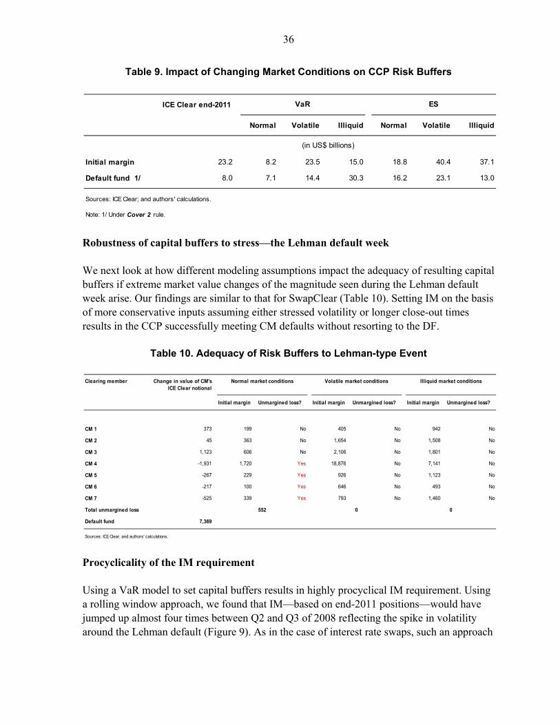
36

Table 9. Impact of Changing Market Conditions on CCP Risk Buffers

Robustness of capital buffers to stress—the Lehman default week We next look at how different modeling assumptions impact the adequacy of resulting capital buffers if extreme market value changes of the magnitude seen during the Lehman default week arise. Our findings are similar to that for SwapClear (Table 10). Setting IM on the basis of more conservative inputs assuming either stressed volatility or longer close-out times results in the CCP successfully meeting CM defaults without resorting to the DF.

Table 10. Adequacy of Risk Buffers to Lehman-type Event

Procyclicality of the IM requirement Using a VaR model to set capital buffers results in highly procyclical IM requirement. Using a rolling window approach, we found that IM—based on end-2011 positions—would have jumped up almost four times between Q2 and Q3 of 2008 reflecting the spike in volatility around the Lehman default (Figure 9). As in the case of interest rate swaps, such an approach

ICE Clear end-2011

Normal Volatile Illiquid Normal Volatile Illiquid

Initial margin 23.2 8.2 23.5 15.0 18.8 40.4 37.1

Default fund 1/ 8.0 7.1 14.4 30.3 16.2 23.1 13.0

Sources: ICE Clear; and authors' calculations.

Note: 1/ Under Cover 2 rule.

VaR ES

(in US$ billions)

Clearing member Change in value of CM's ICE Clear notional

Initial margin Unmargined loss? Initial margin Unmargined loss? Initial margin Unmargined loss?

CM 1 373 199 No 405 No 942 No

CM 2 45 363 No 1,654 No 1,508 No

CM 3 1,123 606 No 2,106 No 1,801 No

CM 4 -1,931 1,720 Yes 18,876 No 7,141 No

CM 5 -267 229 Yes 926 No 1,123 No

CM 6 -217 100 Yes 646 No 493 No

CM 7 -525 339 Yes 793 No 1,460 No

Total unmargined loss

Default fund 7,369

Sources: ICE Clear; and authors' calculations.

Normal market conditions Volatile market conditions Illiquid market conditions

552 0 0

37

to risk management exacerbates the adverse impact of the initial shock on volatility in market values of exposures and on the liquidity of derivatives instruments and collateral.

Figure 9. ICE Clear Initial Margin Using Rolling Daily Returns and Volatilities

Source: Authors’ calculations.

VI. POLICY IMPLICATIONS

Mandatory clearing of standardized OTC-D trades is motivated by its scope for enhancing netting potential, ensuring more secure and comprehensive margining of risk exposures, and increasing transparency regarding the amount, and distribution, of outstanding risk exposures. These factors, individually and in combination, may result in a considerable reduction in the quantum of counterparty credit risk in the OTC-D market. Consequently, it is expected that mandatory clearing will result in a reduction in the shock transmission potential of OTC-D trading relative to a situation where uncleared bilateral trades are preeminent. Some of these benefits are, however, predicated on a market structure wherein a small number of CCPs clear the lion’s share of standardized OTC-D contracts globally. Indeed, from the perspective of maximizing netting potential, Duffie and Zhu (2011) have demonstrated that the efficient market structure is one where a single global CCP clears all standardized OTC-D trades. While no single OTC-D CCP dominates global clearing across all risk products, the ground reality is of one CCP dominating global clearing within some of the most important product classes. These individual CCPs are globally systemically important and, barring a material change, mandatory clearing is set to increase their potential as financial shock transmitters.

0

10

20

30

2007Q1 2007Q2 2007Q3 2007Q4 2008Q1 2008Q2 2008Q3 2008Q4 2009Q1 2009Q2 2009Q3 2009Q4

(in U.S.$ billions)

7.5

(in U.S.$ billions)

7.5

(in U.S.$ billions)

7.5

26.7

11.8

38

From the perspective of financial stability policy, therefore, it is imperative that CCPs’ risk management practices and the prudential standards that apply to them are adequately comprehensive and conservative. The calculation of adequate risk buffers ought to be made on a basis that is as conservative as that governing the calculation of prudential charges for similar risks assumed by the CCP’s CMs in other parts of their portfolios. Otherwise, opportunities for regulatory arbitrage may open up which, in turn, could eventually lead to the accumulation of higher levels of systemic risk in the cleared OTC-D space. In this context, our results raise issues for prudential authorities that are similar to those being discussed in the context of the capitalization of banks’ exposures to market and counterparty credit risk held in their trading books. A first set of issues concerns the sizing of the CCP’s exposures to CMs. Capital requirements are, expectedly, particularly sensitive to the size of CMs’ net positions. Defining netting sets across multiple risk factor classes enables CCPs to offset exposures to CMs via internal model-implied bases relationships across currencies, maturities and indexes-to-SN obligors. This likely plays a vital role in lowering the IM and DF. Our results indicate that narrowing netting sets to permit offsetting only within individual risk factor classes—as in the Basel 2.5 standardized approach—would raise CCP capital requirements significantly unless model-implied netting primarily reflects direct offsets. This is one of the reasons why, in its fundamental review of banks’ trading books, the BCBS is giving consideration to arguments for compartmentalizing the portfolio models to limit offsetting that can occur between major risk factor classes. The reasoning behind this is the prudence in limiting the risk of variable correlation between different risk factors over time. A similar approach is worth considering for CCPs. In the case of A-IRB banks—particularly the G-SIBs—the fundamental review of the trading book has also deliberated the pros and cons of using the standardized approach to set a floor for capital requirements.29 This issue is, in our view, also relevant to the calculation of CCPs’ risk buffers. In this context, the BCBS Level 3 trading book reviews offer the lesson that it is important to limit the choice of methodology and standardized histories so as to have a consistent floor structure across CCPs. A second issue is the sensitivity of the capital requirement to the methodology of calibrating key risk parameter inputs. IM and DF corresponding to a given level of risk tolerance increase significantly when we move away from point-in-time towards a stress-period calibration of the volatility of standardized returns on OTC-D contracts. Similarly, accounting for the fact that it takes longer to close-out positions during times of stress has a

29 BCBS (2012).

39

first-order impact on CCP risk buffers for both interest rate swaps and CDS. Our results demonstrate the value of having CCPs use a stress period calibration. Risk buffers that correspond to the use of point-in-time risk parameter inputs into CCPs’ models can be procyclical. Moving instead to stress period parameter calibration appears to result in risk buffers that are substantially higher, and thus, more comfortably cover losses during tail events like the Lehman default. Moreover, use of this more conservative approach to set IM would also result in stability of the IM requirement in the face of a wide range of shocks. This would result in less pressure on CMs’ liquidity reserves that can be deployed to meet refinancing gaps elsewhere on the balance-sheet during times of stress. From a policy perspective, this underscores the importance of mandating by regulation the use of stress period inputs of returns, the volatility of returns, and instrument liquidity in CCPs’ risk models. Doing so would make CCPs, CMs and their clients more resilient to unexpected shocks and tail events as capital buffers will be resized to be sufficient under extreme stress. It will also have the benefit of reducing procyclicality of IM requirements which will reduce pressure on banks’ liquidity reserves when they need them the most. As a first step in this process, one may want to consider advocating a hypothetical portfolio to be run by all CCPs. The portfolio design would be structured to reveal the degree of offsetting through gross versus net position VaR and the variation from choice of data and parameterization of the VaR. A third issue concerns the choice of metric for risk measurement and tolerance. This is especially important for CDS clearing where—owing to the presence of JtD risk—choosing a tail risk loss measure such as ES raises IM and DF requirements significantly relative to VaR. The principle benefit of using a risk tolerance level built on ES instead of VaR would probably arise from the response of CMs who will have a greater incentive to redesign their portfolio of cleared OTC-D trades toward a safer one in order to avoid the sharp increases in capital costs.30 We conclude with a parting thought regarding the existing philosophy underlying the approach of prudential authorities to risk management standards of OTC-D CCPs. Standard setting bodies have heretofore eschewed a detailed and prescriptive approach to the specification of detailed standards or methodologies for calculating capital requirements for these financial market infrastructures. And, the transcription of these standards into national regulation has, correspondingly, yet to yield the establishment of standardized methodologies to the calculation of risk buffers that could set a benchmark against which to evaluate the CCPs’ model-implied risk buffers. Part of the reason for this could be that loss sharing

30 Yamai and Yoshiba (2002) demonstrate that the primary benefit of compelling banks to use ES instead of VaR is that the ES-optimal portfolio carries considerably lower tail risk relative to the VaR-optimal portfolio.

40

arrangements vary widely across CCPs at the moment in terms of the distribution of the burden represented by the risk buffers on CMs and their clients. CCPs that assign greater weight to their IM buffer lower the mutualization component and the effective burden on CMs relative to CCPs that assign greater weight to the DF. Nonetheless, given the growing global systemic importance of some CCPs, there are considerable benefits from adopting a more proactive approach to international standards and prudential regulation in this area. Greater disclosure by CCPs of their risk models would be a first step in this process.

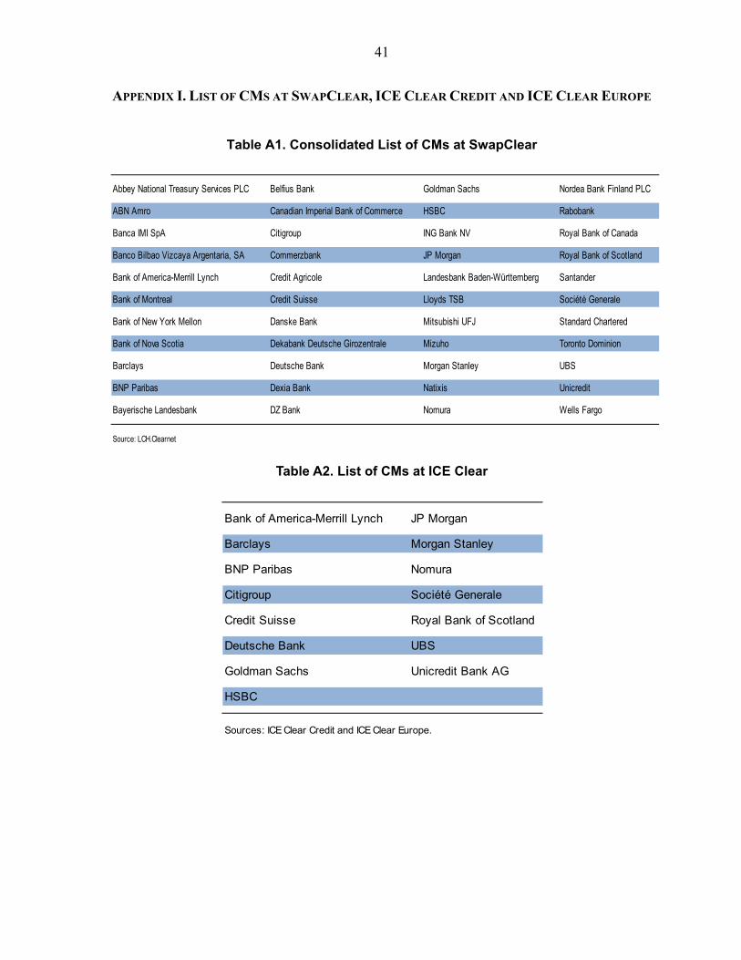
41

APPENDIX I. LIST OF CMS AT SWAPCLEAR, ICE CLEAR CREDIT AND ICE CLEAR EUROPE

Table A1. Consolidated List of CMs at SwapClear

Table A2. List of CMs at ICE Clear

Abbey National Treasury Services PLC Belfius Bank Goldman Sachs Nordea Bank Finland PLC

ABN Amro Canadian Imperial Bank of Commerce HSBC Rabobank

Banca IMI SpA Citigroup ING Bank NV Royal Bank of Canada

Banco Bilbao Vizcaya Argentaria, SA Commerzbank JP Morgan Royal Bank of Scotland

Bank of America-Merrill Lynch Credit Agricole Landesbank Baden-Württemberg Santander

Bank of Montreal Credit Suisse Lloyds TSB Société Generale

Bank of New York Mellon Danske Bank Mitsubishi UFJ Standard Chartered

Bank of Nova Scotia Dekabank Deutsche Girozentrale Mizuho Toronto Dominion

Barclays Deutsche Bank Morgan Stanley UBS

BNP Paribas Dexia Bank Natixis Unicredit

Bayerische Landesbank DZ Bank Nomura Wells Fargo

Source: LCH.Clearnet

Bank of America-Merrill Lynch JP Morgan

Barclays Morgan Stanley

BNP Paribas Nomura

Citigroup Société Generale

Credit Suisse Royal Bank of Scotland

Deutsche Bank UBS

Goldman Sachs Unicredit Bank AG

HSBC

Sources: ICE Clear Credit and ICE Clear Europe.

42

APPENDIX II. MODELING CREDIT SPREADS The residuals of the standardized returns of 30 cleared CDS contracts do not follow a normal distribution nor can their behavior be adequately described by a t–distribution owing to fat-tails. This is so for those contracts where the time series of daily returns exhibits zero variance for long periods of time. This is seen; for e.g., in the time series of daily returns on CDS contracts on two SN obligors, Valero Energy and Verizon (Figure 10).

Figure 10. Comparing Daily Returns on CDS on Two SN Obligors

Source: Authors’ calculations.

Consequently, it is reasonable to fit them with a GARCH model with time varying conditional variance. While searching for an appropriate family of distributions to fit the time series of daily returns of such contracts, we must bear in mind that for a substantially long time, the variance of daily returns for such time series can be zero with the standardized residuals exhibiting extreme values as is the case with the CDS of Verizon Communications (Figure 11).

Figure 11. Comparing Standardized Residuals on CDS on Two SN Obligors

Source: Authors’ calculations.

43

In the literature, a mixture of the Pareto distribution—in the tails—and a kernel smoothed interior is used to fit the residuals as this captures extreme values (Figure 12).

Figure 12. Fitting Residuals Using a Mixed Paretotail and Kernel Smoothed Interior

Source: Authors’ calculations.

In order to fit a copula, the margins of the residuals have to follow a uniform distribution.31 This is difficult to reconcile with fitting of a mixed Paretotail distribution, of time series such as the Verizon CDS. Whereas the random numbers generated from the copula will have uniform margins, about 99 percent of the margins generated from the mixed Paretotail distribution are concentrated in the region [0.5. 0.7] (Figure 13). Applying the uniformly distributed margin simulated from the copula to the fitted Paretotail distribution (Figure 12) leads to a larger proportion of the simulated residuals staying in the upper and lower 10 percent quantile. Therefore, the simulated data will put a larger weight on the tails, which strongly contradicts with the pattern of real data, which is concentrated in the [0.5, 0.7] range. Consequently, we use a non-parametric distribution that generates margins of the residuals closer to the uniformly distributed margins simulated by the copula (Figure 14). This is especially so for the tail wherein the weights, either from the simulated data or from the real data are close. Therefore, the simulated margins will no longer lead to a larger number of tailed residuals than in the real data. While the distribution of the margins under the non-parametric distribution still does not follow the uniform distribution in the range [0.3, 0.7], where the real data is concentrated in the [0.5, 0.55] range and the simulated data are

31 A discussion of modeling issues can be found in Marcucci (2005).

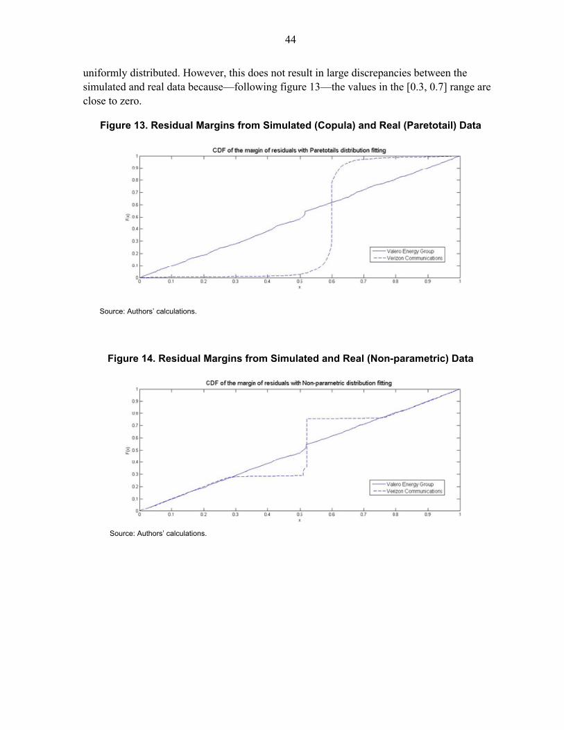
44

uniformly distributed. However, this does not result in large discrepancies between the simulated and real data because—following figure 13—the values in the [0.3, 0.7] range are close to zero.

Figure 13. Residual Margins from Simulated (Copula) and Real (Paretotail) Data

Source: Authors’ calculations.

Figure 14. Residual Margins from Simulated and Real (Non-parametric) Data

Source: Authors’ calculations.

45

REFERENCES

Bank for International Settlements (2012), “Semi-Annual OTC-Derivatives Statistics as of end-December 2011”, September, Basel: Bank for International Settlements.

Basel Committee on Banking Supervision (2011), Revisions to the Basel II Market Risk

Framework, (December 31, 2011 update), Publication 193, Basel: Bank for International Settlements.

——— (2012), Fundamental Review of the Trading Book, (Consultative Document),

Publication 219, Basel: Bank for International Settlements. Begeneau, J., M. Piazzesi and M. Schneider (2012), “Banks’ Risk Exposures”, Working

Paper, Department of Economics, Stanford University. Chen, K., M. Fleming, J. Jackson, A. Li, and A. Sarkar (2011), “An Analysis of CDS

Transactions: Implications for Public Reporting”, Staff Report 517, New York, N.Y.: Federal Reserve Bank of New York.

Committee on Payments and Settlements Systems and International Organization of

Securities Commissions (2012), Principles for Financial Market Infrastructures, Publication 101a, Basel: Bank for International Settlements.

Duffie, D. and K. Singleton (2003), Credit Risk: Pricing, Measurement, and Management,

Princeton, N.J.: Princeton University Press. Duffie, D. and H. Zhu (2011), “Does a Central Clearing Counterparty Reduce Counterparty

Risk?,” Review of Asset Pricing Studies, vol. 1, pp. 74-95. Financial Stability Board (2012), Update of Group of Global Systemically Important Banks,

November, Basel. Available at: www.financialstabilityboard.org/publications/r_121031ac.pdf

Fleming, M., J. Jackson, A. Li, A. Sarkar, and P. Zobel (2012), “An Analysis of OTC Interest

Rate Derivatives Transactions: Implications for Public Reporting”, Staff Report 557, New York, N.Y.: Federal Reserve Bank of New York.

Gorton, G. and R. Rosen (1995), “Banks and Derivatives”, NBER Macroeconomics Annual

1995, vol. 10, pp. 299-339. Gregory, J. (2012), Counterparty Credit Risk: The New Challenge for Global Financial

Markets, West Sussex, U.K.: John Wiley and Sons.

46

Heller, D. and N. Vause (2012), “Collateral Requirements for Mandatory Clearing of Over-the-Counter Derivatives”, Working Paper 373, Basel: Bank for International Settlements.

Hull, J. and A. White (1998), “Incorporating Volatility Updating into the Historical Simulation Method for Value-at-Risk”, Journal of Risk, vol. 1, pp. 5-19.

InterContinental Exchange (2012a), ICE Clear Credit Clearing Rules, Chicago, IL. ——— (2012b), ICE CDS Margin Calculator, Chicago, IL. ——— (2012c), Portfolio Approach to CDS Margining and Index Decomposition

Methodology, Chicago, IL. International Monetary Fund (2010), “Making Over-the-Counter Derivatives Safer: The Role

of Central Counterparties”, chapter 3 of the Global Financial Stability Report, April, Washington, D.C.

——— (2012), Global Financial Stability Report, Statistical Appendix, October,

Washington, D.C. International Monetary Fund, Bank for International Settlements and Financial Stability

Board (2009), Guidance to Assess the Systemic Importance of Financial Institutions, Markets and Instruments: Initial Considerations, October, Report to the G20 Finance Ministers and Central Bank Governors, Washington, D.C. and Basel. Available at: www.imf.org/external/np/g20/pdf/100109.pdf

LCH.Clearnet (2012a), “LCH.Clearnet—Initial Margins”, London, U.K. ——— (2012b), “SwapClear Rules and Regulations Update”, Circular 3143, April 26,

London, U.K. Available at: http://www.lch.co.uk/member_notices/circulars/2012-04-26_3.asp

Marcucci, J. (2005), “Forecasting Stock Market Volatility with Regime-Switching GARCH

Models”, Studies in Nonlinear Dynamics and Econometrics, vol. 9, pp. 1-53. O’Kane, D. and S. Turnbull (2003), “Valuation of Credit Default Swaps”, Lehman Brothers

Fixed Income Quantitative Credit Research, April. Scarlata, J., E. Gaston, J. Kiff, and J. Surti (2012), “Over-the-Counterparty Derivative

Central Counterparties”, Quarterly Report on Systemically Important Financial Institutions (Non-Banks), January, Washington, D.C.: International Monetary Fund.

Yamai, Y. and T. Yoshiba (2002), “Comparative Analyses of Expected Shortfall and Value-

at-Risk under Market Stress, Monetary and Economic Studies, vol. 20, pp. 181-237.