Capital Input in OECD Agriculture:A Multilateral Comparison

V. Eldon Ball, W. A. Lindamood, and Richard NehringEconomic Research Service

U.S. Department of Agriculture1800 M Street, NW

Washington, DC 20036-5831USA

Carlos San Juan Department of Economics

Universidad Carlos III de Madrid28903 Madrid, Spain

Capital Input in OECD Agriculture: A Multilateral Comparison

Overview

• We construct capital accounts for the agricultural sector in fourteen OECD countries

• In doing so we make a distinction between declines in efficiency of an asset and economic depreciation

• The efficiency of a used asset relative to that when new is defined as the marginal rate of substitution of the used asset for the new one

• Economic depreciation is the decline in price of a capital good with age, so that estimates of depreciation depend on the relative efficiencies of assets of different ages

• Economists frequently assume that relative efficiency declines geometrically

• If decay is a characterized by a geometric series, then depreciation is also geometric and occurs at the same constant rate

• Under this assumption, no distinction need be made when measuring capital

• In general, however, efficiency decline and depreciation are different

• This results in two distinct but related measures of capital--capital as a factor of production and as a measure of wealth

Capital as a Factor of Production

• The starting point for construction of a measure of capital input is the measurement of capital stock for each asset type

• For depreciable assets, the perpetual inventory method is used to derive capital stock from data on investment in constant prices

• We estimate the stock of land implicitly as the ratio of the value of land in farms to the price index of land

• The next step in developing measures of capital input is to construct estimates of prices of capital services

• Implicit rental prices for each asset are based on the correspondence between the purchase price of the asset and the discounted value of future service flows derived from that asset

• Our estimates of capital input incorporate the same data on relative efficiencies of capital goods into estimates of both capital stock and capital rental prices, so that the requirement for internal consistency of measures of capital input is meet

Depreciable Capital

• We represent depreciable capital stock at the end of each period, say Kt, as the sum of past investments, each weighted by its relative efficiency, say dt:

• We normalize initial efficiency d0 at unity and assume that relative efficiency decreases so that:

• We also assume that every capital good is eventually retired or scrapped so that relative efficiency declines to zero:

I d = K -t=0

t

,10 d Tdd ,...,1,0,01

0lim

d

• The decline in efficiency of capital goods gives rise to needs for replacement in order to maintain the productive capacity of the capital stock

• The proportion of a given investment to be replaced at age , say m , is equal to the decline in efficiency from age -1 to age :

• These proportions represent mortality rates for capital goods of different ages

• Replacement requirements, say Rt, are represented as a weighted sum of past investments

where the weights are the mortality rates

Tddm ,...,1,1

1 tt ImR

• To estimate replacement, we must introduce an explicit description of the decline in efficiency

• The efficiency function, d, may be expressed in terms of two parameters, the service life of the asset, say L, and a curvature or decay parameter, say β

• One possible form for the efficiency function is given by:

L ,0 = d

L 0 ,) - L ( / ) - L ( = d

• This function is a form of a rectangular hyperbola that provides a general model incorporating several types of depreciation as special cases

•The value of β is restricted only to values less than or equal to one

• For values of β greater than zero, the function d approaches zero at an increasing rate

• For values less than zero, d approaches zero at a decreasing rate

• Two studies (Penson, Hughes, and Nelson; Romain, Penson, and Lambert) provide evidence that efficiency decay occurs more rapidly in the later years of service, corresponding to a value of β in the zero-one interval

• The efficiency of a structure declines very slowly over most of its service life until a point is reached where the cost of repairs exceeds the increased service derived from the repairs, at which point the structure is allowed to depreciate rapidly (β=0.75)

• The decay parameter for durable equipment (β=0.5) assumes that its decline in efficiency is more uniformly distributed over the asset’s service life

• The other variable in the efficiency function is the asset lifetime L

• For each asset type, there exists some mean service life L around which there exists some distribution of the actual service lives

• It is assumed that this distribution may be accurately depicted by the standard normal distribution truncated at points two standard deviations before and after the mean service life

• An aggregate efficiency function is then constructed as a weighted sum of individual efficiency functions (corresponding to various values of L) using as weights their frequency of occurrence

Capital Rental Prices

• The behavioral assumption underlying the derivation of the rental price of capital is that firms buy and sell assets so as to maximize the present value of the firm

• This implies that firms will add to the capital stock so long as the present value of the net revenue generated by an additional unit of capital exceeds the purchase price of the asset:

• To maximize net present value, firms will continue to add to capital stock until this equation holds as an equality:

where c is the implicit rental price of capital

w> )r + (1 KR w-

K

y p t-t

1=t

c)r + (1 KR w r + wr =

K

y p t-t

1=t

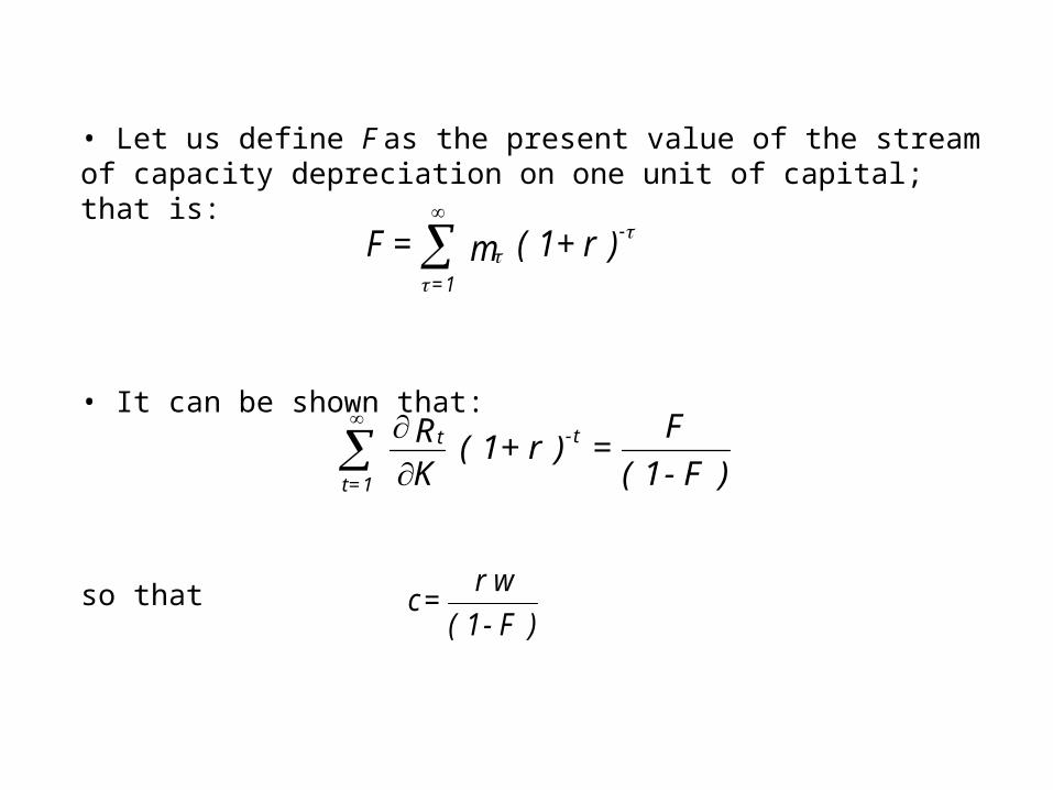
• Let us define F as the present value of the stream of capacity depreciation on one unit of capital; that is:

• It can be shown that:

so that

) r + 1 ( m = F -

1=

) F - 1 (

F = ) r + 1 (

KR t-t

1=t

) F - 1 (

wr = c

Relative Levels of Capital Input

• Comparisons of levels of capital input among countries require data on relative prices of capital input

• A price index that converts the ratio of the nominal value of capital service flows between two countries into an index of relative real capital input is referred to as a purchasing power parity of the currencies of the two countries

• The appropriate purchasing power parity for new capital goods is the purchasing power parity for the corresponding component of investment goods output

• To obtain the purchasing power parities for capital input, we must take into account the flow of capital services per unit of capital stock in each country

• This is accomplished by multiplying the purchasing power parity for investment goods for any country by the ratio of the price of capital input for that country relative to the United States

• This yields relative prices in each country expressed in terms of national currency per dollar

• Finally, we translate the purchasing power parities into relative prices in dollars by dividing by the exchange rate

Land

• To estimate the stock of land in each country, we construct time series price indexes of land in farms

• The stock of land is then constructed implicitly as the ratio of the value of land in farms to the time series price index

• Differences in the relative efficiencies of land across countries prevent the direct comparison of observed prices

• To account for these differences, indexes of relative prices of land are constructed using hedonic methods

• Under the hedonic approach, the price of land is a function of thecharacteristics it embodies

• Therefore, the hedonic function may be expressed as W=W(X,D), where W represents the price of land, X is a vector of characteristics, and D is a vector of other variables • Characteristics include soil acidity, salinity, and moisture stress, among others

• In areas with moisture stress, agriculture is not possible without irrigation, hence irrigation is included as a separate variable

• Because irrigation mitigates the negative impact of acidity on plant growth, the interaction between irrigation and soil acidity is also included in the hedonic regression

• In addition to environmental attributes, we also include a “population accessibility” score for each region in each country

• These indexes are constructed using a gravity model of urban development, which provides a measure of accessibility to population concentrations

• A gravity model accounts for both population density and distance from that population center

• The index increases as population increases and/or distance from the population center decreases

• Other variables (denoted by D) include country dummy variables which capture price effects other than quality

• Most empirical studies adopt the semilog or double-log form of the hedonic price function

• However, economic theory places few if any restrictions on the functional form of the hedonic price function

• We adopt a generalized linear form where the dependent variable and each of the continuous independent variables are represented by the Box-Cox transformation

• This mathematical expression can assume both linear and logarithmic forms, as well as intermediate non-linear forms

Capital Input, 1973-2002

Prices of capital input relative to U.S. in 1996

Year Belgium Denmark Germany Greece Spain France Ireland Italy Luxem- bourg

Nether- lands

Portugal Sweden United

Kingdom United States

1973 0.4285 0.2496 0.4923 0.9983 0.4431 0.3047 0.2456 0.4548 0.2872 0.4584 0.1788 0.3436 0.3506 0.2744 1974 0.4768 0.3645 0.5723 0.7857 0.4833 0.3937 0.3927 0.6043 0.3364 0.6512 0.2131 0.3834 0.3840 0.2752

1975 0.4347 0.3127 0.4790 0.7156 0.4568 0.4537 0.3324 0.5046 0.2569 0.5414 0.2075 0.4634 0.3286 0.2736

1976 0.4684 0.3385 0.5264 0.6302 0.3853 0.3807 0.3549 0.4525 0.3203 0.5130 0.2086 0.4701 0.3122 0.2812 1977 0.6176 0.4119 0.7211 0.6104 0.3658 0.3788 0.4255 0.5041 0.4042 0.7727 0.2501 0.4751 0.3225 0.3336

1978 0.8774 0.6062 0.8123 0.6752 0.3889 0.4395 0.4889 0.6352 0.5678 1.0461 0.2657 0.4916 0.3953 0.4156

1979 1.0806 0.7136 1.0937 0.9366 0.5016 0.4787 0.4940 0.8858 0.7665 1.3601 0.2544 0.5561 0.5899 0.5281

1980 1.6598 0.7339 1.3509 1.7038 0.6118 0.5838 0.5203 0.6055 1.2697 1.6252 0.3123 0.7161 0.7241 0.6895 1981 1.8156 0.6321 1.6223 2.3592 0.7052 0.7565 0.5865 0.6734 1.5712 1.5804 0.3198 0.7149 0.7211 0.9980

1982 1.4103 0.6395 1.4324 2.3332 0.8194 0.8294 0.5275 0.5873 1.1640 1.4049 0.3966 0.6460 0.8005 0.9662

1983 1.1040 0.5668 1.1876 1.6915 0.6987 0.6777 0.6313 0.5556 0.8099 1.1236 0.5615 0.5881 0.7655 1.0809

1984 1.0188 0.4529 1.1087 1.1456 0.8147 0.4911 0.5626 0.4808 0.7508 1.0460 0.5019 0.5522 0.7698 1.2679 1985 0.9232 0.4474 1.0357 0.7628 0.6198 0.4880 0.7638 0.4434 0.7433 1.0909 0.3745 0.5907 0.6568 1.0343

1986 1.0184 0.6117 1.2298 0.8490 0.9679 0.6679 1.0229 0.6170 0.8050 1.4728 0.6412 0.7273 0.7471 0.7485

1987 1.1306 0.8694 1.3033 1.0269 1.2545 0.8857 1.1695 0.8100 0.9800 1.8774 0.7711 0.8659 0.9417 0.8188

1988 1.3136 1.0361 1.4962 1.3849 1.9546 1.0769 1.4783 0.9493 1.2813 2.2590 0.7622 0.9939 1.1716 0.8558 1989 1.4623 0.9828 1.7569 1.6769 2.2776 1.1148 1.3853 1.0580 1.7136 2.3911 0.7348 1.0188 1.1467 0.8452

1990 1.7606 1.4008 2.5711 2.0704 3.0408 1.5528 1.4565 1.3600 2.8683 3.0504 0.8973 1.3033 1.2837 0.8823

1991 1.9065 1.4321 2.5842 2.5112 2.9475 1.5228 1.3472 1.6170 3.0636 3.0194 0.7460 1.2981 1.1862 0.8392

1992 2.0308 1.4187 2.0108 2.4902 2.5904 1.5963 1.5073 1.5353 3.9048 3.1064 0.4884 1.2624 1.2690 0.8012 1993 1.5343 1.1695 1.4391 2.4089 1.7488 1.2621 1.2209 1.1908 2.3984 2.5701 0.2364 0.9122 1.3332 0.7984

1994 1.5789 1.3172 1.6424 2.2866 1.7334 1.4053 1.0382 1.2319 1.9461 2.6867 0.3839 0.9207 1.4633 0.9073

1995 2.0608 1.7559 2.0896 2.2592 2.3010 1.6598 1.8841 1.3483 2.8551 3.3262 0.5148 1.1025 1.7431 0.9707

1996 1.8974 1.6123 1.8548 2.1689 2.2303 1.5230 1.6716 1.4323 2.8245 3.0326 0.6325 1.0943 1.6044 1.0000 1997 1.6199 1.2315 1.5645 1.7554 1.9030 1.2611 1.5712 1.2750 2.2949 2.7086 0.5784 0.9151 1.3062 1.0617

1998 1.4224 1.0194 1.4647 2.1207 1.8828 1.1636 1.0738 1.2291 1.8409 2.5897 0.5214 0.8652 1.1646 0.9511

1999 1.3414 1.0796 1.3628 1.8772 1.7670 1.1600 0.8951 1.2711 2.0966 2.2673 0.5832 0.8539 0.9917 1.1210

2000 1.4080 1.0686 1.4548 1.2694 1.4115 1.1391 1.0049 1.0758 2.8064 2.1083 0.7094 0.7557 0.9824 1.1542 2001 1.3156 1.0106 1.5345 1.2526 1.1754 1.0945 1.0452 1.1203 2.5835 2.0095 0.5462 0.7076 0.8763 0.9231

2002 1.3105 1.0129 1.4434 1.2862 1.0967 1.0474 0.8691 1.1137 2.4685 2.1059 0.4421 0.8459 0.8628 0.8528

Capital input (millions of 1996 U.S. dollars)

Year Belgium Denmark Germany 1/ Greece Spain France Ireland Italy Luxem- bourg

Nether- lands

Portugal Sweden United

Kingdom United States

1973 710 1058 10902 1345 5291 9191 929 7918 163 1410 334 1322 5900 50162

1974 741 1158 10994 1354 5340 9588 971 8116 164 1473 359 1305 5957 51455

1975 773 1235 11016 1371 5317 9932 968 8299 166 1536 387 1300 5979 52753

1976 780 1306 11023 1404 5333 10263 984 8470 167 1576 422 1316 5941 53556

1977 791 1380 11087 1414 5356 10607 1017 8702 167 1616 454 1338 5912 54654

1978 805 1439 11136 1442 5410 10836 1057 8938 164 1682 490 1338 5903 55478

1979 825 1503 10946 1445 5497 11073 1099 9125 165 1756 519 1326 5907 56454

1980 831 1567 11006 1459 5594 11251 1144 9419 165 1831 553 1316 5906 57328

1981 827 1582 11012 1463 5740 11372 1169 9814 163 1870 594 1286 5844 57129

1982 822 1570 10965 1464 5800 11478 1194 10083 162 1899 626 1259 5817 56507

1983 819 1560 10916 1470 5854 11573 1203 10150 163 1932 636 1242 5830 55344

1984 813 1555 10914 1473 5915 11608 1205 10235 164 1980 640 1227 5888 54218

1985 808 1559 10874 1491 5949 11681 1207 10385 163 2001 639 1222 5953 53054

1986 802 1580 10827 1500 5951 11646 1207 10417 162 2011 637 1201 5974 51332

1987 801 1600 10767 1496 5971 11560 1226 10425 160 2021 654 1173 5980 49457

1988 800 1602 10719 1486 5989 11491 1212 10407 158 2029 676 1150 5991 48137 1989 796 1589 10676 1484 5963 11654 1196 10258 158 2034 708 1137 5984 46936

1990 793 1594 10678 1479 5915 11732 1191 10107 159 2051 735 1131 5982 46012

1991 791 1596 11321 1469 5829 11768 1195 10061 158 2069 760 1115 5969 45276

1992 782 1582 11304 1474 5786 11750 1195 10039 159 2088 787 1085 5932 44419

1993 785 1557 11312 1472 5698 11625 1196 9981 160 2109 806 1049 5932 43561

1994 777 1516 11231 1471 5615 11521 1187 9900 159 2099 826 1015 5944 42916

1995 765 1502 11131 1470 5519 11469 1194 9881 159 2093 841 1004 5962 42358

1996 757 1498 11046 1467 5462 11464 1199 9891 157 2037 862 995 6013 41786

1997 751 1479 11043 1451 5489 11589 1219 9914 155 2051 885 979 6040 41416

1998 748 1487 10979 1417 5472 11659 1221 9950 154 2046 911 978 6020 41179

1999 745 1484 10839 1400 5429 11900 1227 10043 154 2061 926 974 5936 41032

2000 745 1478 10792 1378 5379 11998 1229 10101 153 2075 948 978 5800 40763

2001 745 1482 10771 1354 5348 12119 1228 10127 152 2085 965 984 5750 40513

2002 748 1496 10703 1330 5304 12238 1226 10175 152 2110 978 988 5666 40407

1/ Includes former East Germany beginning in 1991.

Concluding Remarks

• Our objective is to provide a farm-sector comparison of levels of capital input among OECD countries

• This comparison begins with estimating the capital stock and rental price for each asset class for each country

• The same patterns of decline in efficiency are used for both capital stock and the rental price of each asset, so that the requirement for internal consistency of measures of capital input is met

• In order to compare levels of capital input among countries, we require conversion factors that reflect the comparative value of their currencies

• We make use of purchasing power parities for investment goods output, taking into account the flow of capital services per unit of capital stock

• These conversion factors are used to express the value of capital service flows in each country in a common unit

• As a final step, we form indexes of relative prices of capital input among countries by taking the ratio of the purchasing power parity and the exchange rate

• This allows us to decompose the values of capital services into price and quantity components