Capacity and Performance Analysis ofAdvanced Multiple Antenna

Communication Systems

A THESIS SUBMITTED TO THE UNIVERSITY COLLEGE LONDONIN PARTIAL FULFILLMENT OF THE REQUIREMENTS FOR THE

DEGREE OF DOCTOR OF PHILOSOPHY

By

Caijun Zhong

Department of Electronic and Electrical Engineering

University College London

London, United Kingdom

March 2010

Declaration

I, Caijun Zhong, confirm that the work presented in this thesis is my own. Where information has been

derived from other sources, I confirm that this has been indicated in the thesis.

Acknowledgments

Foremost, I thank my supervisor, Dr. Kai-Kit Wong, for giving me the opportunity to be a part of his

research group. I am greatly indebted to him for his full support, constant encouragement, and guidance

in the past three years. I just hope I can live up to his expectations in my future career.

I am very grateful to Dr. Gan Zheng, who has helped me a lot in the beginning of my PhD study. Special

thanks to Dr. Shi Jin for introducing random matrix theory as well as collaborating on various topics,

working with Shi has been fantastic. My thanks also goes to Dr. McKay Matthew, for the insightful

discussion and collaboration.

Finally, I would like to thank my parents, my sister and brother-in-law for their love and support.

Abstract

Multiple-input multiple-output (MIMO) antenna systems have been shown to be able to substantially

increase date rate and improve reliability without extra spectrum and power resources. The increasing

popularity and enormous prospect of MIMO technology calls for a better understanding of the perfor-

mance of MIMO systems operating over practical environments. Motivated by this, this thesis provides

an analytical characterization of the capacity and performance of advanced MIMO antenna systems.

First, the ergodic capacity of MIMO Nakagami-m fading channels is investigated. A unified way of

deriving ergodic capacity bounds is developed under the majorization theory framework. The key idea is

to study the ergodic capacity through the distribution of the diagonal elements of the quadratic channel

HH† which is relatively easy to handle, avoiding the need of the eigenvalue distribution of the channel

matrix which is extremely difficult to obtain. The proposed method is first applied on the conventional

point-to-point MIMO systems under Nakagami-m fading, and later extended to the more general dis-

tributed MIMO systems.

Second, the ergodic capacity of MIMO multi-keyhole and MIMO amplify-and-forward (AF) dual-hop

systems is studied. A set of new statistical properties involving product of random complex Gaussian

matrix, i.e., probability density function (p.d.f.) of an unordered eigenvalue, p.d.f. of the maximum

eigenvalue, expected determinant and log-determinant, is derived. Based on these, analytical closed-

form expressions for the ergodic capacity of the systems are obtained and the connection between the

product channels and conventional point-to-point MIMO channels is also revealed.

Finally, the effect of co-channel interference is investigated. First, the performance of optimum com-

bining (OC) systems operating in Rayleigh-product channels is analyzed based on novel closed-form

expression of the cumulative distribution function (c.d.f.) of the maximum eigenvalue of the resultant

channel matrix. Then, for MIMO Rician channels and MIMO Rayleigh-product channels, the ergodic ca-

pacity at low signal-to-noise ratio (SNR) regime is studied, and the impact of various system parameters,

such as transmit and receive antenna number, Rician factor, channel mean matrix and interference-to-

noise-ratio, is examined.

Publications

The following is a list of journal and conference publications produced during my Ph.D. study.

Journal papers

1. C. Zhong, K. K. Wong, and S. Jin, “Capacity bounds for MIMO Nakagami-m fading channels”,

IEEE Transactions on Signal Processing, vol. 57, no. 9, pp. 3613–3623, Sep. 2009.

2. C. Zhong, S. Jin, K. K. Wong, and M. R. McKay, “Outage analysis for optimal beamforming

MIMO systems in multi-keyhole channels,” to appear in IEEE Transactions on Signal Process-

ing.

3. S. Jin, M. R. McKay, C. Zhong, and K. K. Wong, “Ergodic capacity analysis of amplify-and-

forward MIMO dual-hop systems,” to appear in IEEE Transactions on Information Theory.

4. C. Zhong, S. Jin, and K. K. Wong, “MIMO Rayleigh-product channels with co-channel interfer-

ence,” IEEE Transactions on Communications, vol. 57, no. 6, pp. 1824–1835, June 2009.

5. C. Zhong, G. Zheng, and K. K. Wong,“Feasibility conditions of linear multiuser MIMO antenna

systems in the asymptotic regime,” IEEE Communications Letters, vol. 11, no. 12, pp. 979–

981, Dec. 2007.

6. C. Zhong, S. Jin, and K. K. Wong, “Dual-hop systems with noisy relay and interference-limited

destination,” to appear in IEEE Transactions on Communications.

Conference papers

1. C. Zhong, K. K. Wong, and S. Jin, “On the Ergodic Capacity of MIMO Nakagami-fading chan-

nels,” in proceedings of IEEE International Symposium on Information Theory (ISIT 2008),

Toronto, Canada, July 2008, pp.131–135.

2. C. Zhong, S. Jin, K. K. Wong, and M. R. McKay, “Performance analysis of transmit beamforming

in multi-keyhole MIMO channels,” IEEE International Conference on Communications (ICC

2009), Dresden, Germany, June 2009, pp. 1–5.

3. S. Jin, M. R. McKay, C. Zhong, and K. K. Wong, “Ergodic capacity analysis of amplify-and-

forward MIMO dual-hop systems,” IEEE International Symposium on Information Theory

(ISIT 2008), Toronto, Canada, July 2008, pp. 1903-1907.

4. C. Zhong, S. Jin, and K. K. Wong, “Performance analysis of a Rayleigh-product MIMO chan-

nel with receiver correlation and cochannel interference,” IEEE International Conference on

Acoustics, Speech and Signal Processing (ICASSP 2008), Las Vegas, USA, March 2008, pp.

2877–2880.

5. C. Zhong, S. Jin, and K. K. Wong, “Low SNR capacity of MIMO channels with a single inter-

ferer,” accepted in IEEE International Workshop on Signal Processing Advances for Wireless

Communications (SPAWC 2009), Perugia, Italy, June 2009, pp. 578–582.

6. C. Zhong, S. Jin, and K. K. Wong, “Outage probability of dual-hop relay channels in the presence

of interference,” IEEE 69th Vehicular Technology Conference (VTC2009-Spring), Barcelona,

Spain, Apr. 2009, pp. 1–5.

7. C. Zhong, S. Jin, K. K. Wong, “Outage Probability Analysis for Systems Using Amplify-and-

Forward Relays with Direct Link,” London Communications Symposium 2009, London, UK,

Sep. 2009.

V

Notations

Here, we introduce the notations adopted in this thesis. Unless otherwise clearly indicated, boldface

upper-case letters generally denote matrices, while boldface lower-case letters generally denote column

vectors.

∈ Belongs to.

∼ Follows certain distribution.

 Majorization relationship.

⊗ Kronecker product.

∆= Defined as.

π 3.1415926∑

Summation symbol∏

Product symbol

∞ Infinite symbol

! Factorial

→ Approach symbol

[H]i,j or Hij (i, j)-th element of matrix H.

0m×n m× n matrix with all elements being zero.

In n× n Identity matrix.

Rm,Cm Real and complex m× 1 vector.

Rm×n, Cm×n Real and complex M ×N matrix.

CN (m,C) Complex circularly symmetric Gaussian vector with mean m and covariance C.

E(·) Expectation.

HT Transpose of matrix H.

H∗ Complex conjugate of matrix H.

H† Conjugate transpose of matrix H.

tr(H) Trace of matrix H.

|H| or det(H) Determinant of square matrix H.

min(x, y) Minimum of x and y.

max(x, y) Maximum of x and y.

VI

In(·) Bessel function of the first kind

B(·, ·) Beta function

U(·, ·, ·) Confluent hypergeometric function of the second kind

ψ(·) Digamma function

exp(·) Exponential function

ex Exponential function

En(·) Exponential integral function of order n

Γ(·) Gamma function

log2(·) Logarithm in base 2.

Gs,tm,n(·) Meijer-G function

Kn(·) Modified Bessel function of the second kind

ln(·) Natural logarithm function√· Square root function

Q(·) Standard Gaussian Q-function

VII

Abbreviations

1G 1st Generation Mobile Communication Systems

2G 2nd Generation Mobile Communication Systems

3G 3rd Generation Mobile Communication Systems

4G 4th Generation Mobile Communication Systems

3GPP-LTE Third Generation Partnership Project

AF Amplify-and-Forward

AWGN Additive White Gaussian Noise

BER Bit Error Rate

BFSK Binary Frequency Shift-Keying

BPSK Binary Phase Shift-Keying

CCI Co-Channel Interference

CDF Cumulative Distribution Function

C-MIMO Co-located MIMO

CSI Channel State Information

CSIT Channel State Information at Transmitter

D-MIMO Distributed MIMO

DSL Digital Subscriber Line

GPRS General Packet Radio Service

GSM Global System for Mobile Communication

IEEE Institute of Electrical and Electronics Engineers

INR Interference to Noise Ratio

LAN Local Area Network

LOS Line of Sight

MAN Metropolitan Area Network

MIMO Multiple Input Multiple Output

MISO Multiple Input Single Output

MMSE Minimum Mean Square Error

MRC Maximum Ratio Combining

OC Optimum Combining

PAM Phase Amplitude Modulation

PAN Personal Area Network

PDF Probability Density Function

RMT Random Matrix Theory

VIII

SDMA Space Division Multiple Access

SISO Single Input Single Output

SIMO Single Input Multiple Output

SM Spatial Multiplexing

SER Symbol Error Rate

SINR Signal to Interference and Noise Ratio

STBC Space Time Block Code

SNR Signal Noise Rate

SVD Singular Value Decomposition

UMTS Universal Mobile Telecommunication System

VBLAST Vertical Bell Laboratories Layered Space Time

WiMAX Worldwide Interoperability for Microwave Access

WAN Wide Area Network

ZMCSCG Zero Mean Circularly Symmetric Complex Gaussian

ZF Zero Forcing

IX

Contents

1 Introduction 1

1.1 Benefits of Wireless Communication . . . . . . . . . . . . . . . . . . . . . . . . . . . . 1

1.2 Current Wireless Networks . . . . . . . . . . . . . . . . . . . . . . . . . . . . . . . . . 2

1.2.1 Wireless PAN . . . . . . . . . . . . . . . . . . . . . . . . . . . . . . . . . . . . 2

1.2.2 Wireless LAN . . . . . . . . . . . . . . . . . . . . . . . . . . . . . . . . . . . 2

1.2.3 Wireless MAN . . . . . . . . . . . . . . . . . . . . . . . . . . . . . . . . . . . 3

1.2.4 Wireless WAN . . . . . . . . . . . . . . . . . . . . . . . . . . . . . . . . . . . 3

1.3 Motivation . . . . . . . . . . . . . . . . . . . . . . . . . . . . . . . . . . . . . . . . . . 4

1.4 Dissertation Contributions and Outline . . . . . . . . . . . . . . . . . . . . . . . . . . . 5

2 Wireless Background 7

2.1 Wireless Communication Systems . . . . . . . . . . . . . . . . . . . . . . . . . . . . . 7

2.1.1 Wireless Fading Channels . . . . . . . . . . . . . . . . . . . . . . . . . . . . . 8

2.1.2 Performance Measures . . . . . . . . . . . . . . . . . . . . . . . . . . . . . . . 9

2.2 MIMO Systems . . . . . . . . . . . . . . . . . . . . . . . . . . . . . . . . . . . . . . . 12

2.2.1 MIMO Channels . . . . . . . . . . . . . . . . . . . . . . . . . . . . . . . . . . 12

2.2.2 Benefits of MIMO Systems . . . . . . . . . . . . . . . . . . . . . . . . . . . . 13

2.2.3 Transmission Schemes . . . . . . . . . . . . . . . . . . . . . . . . . . . . . . . 14

2.2.4 Capacity of MIMO Channels . . . . . . . . . . . . . . . . . . . . . . . . . . . . 16

3 Mathematical Preliminaries 18

3.1 Majorization Theory . . . . . . . . . . . . . . . . . . . . . . . . . . . . . . . . . . . . 18

3.2 RMT . . . . . . . . . . . . . . . . . . . . . . . . . . . . . . . . . . . . . . . . . . . . . 20

3.2.1 Definitions and Preliminary Results . . . . . . . . . . . . . . . . . . . . . . . . 20

3.2.2 New Random Eigenvalue Distribution Results . . . . . . . . . . . . . . . . . . . 21

3.2.3 New Random Determinant Results . . . . . . . . . . . . . . . . . . . . . . . . . 27

3.3 Conclusion . . . . . . . . . . . . . . . . . . . . . . . . . . . . . . . . . . . . . . . . . 30

4 Capacity Bounds for MIMO Nakagami-m Fading Channels 32

4.1 Introduction . . . . . . . . . . . . . . . . . . . . . . . . . . . . . . . . . . . . . . . . . 32

4.2 System Model . . . . . . . . . . . . . . . . . . . . . . . . . . . . . . . . . . . . . . . . 33

4.2.1 MIMO Systems . . . . . . . . . . . . . . . . . . . . . . . . . . . . . . . . . . . 33

4.2.2 Ergodic Capacity . . . . . . . . . . . . . . . . . . . . . . . . . . . . . . . . . . 34

4.3 Capacity Bounds of C-MIMO Nakagami-m Channels . . . . . . . . . . . . . . . . . . . 34

4.3.1 Ergodic Capacity Upper Bounds . . . . . . . . . . . . . . . . . . . . . . . . . . 34

4.3.2 Upper Bound for Large Systems at High SNR . . . . . . . . . . . . . . . . . . . 36

4.3.3 Ergodic Capacity Lower Bounds . . . . . . . . . . . . . . . . . . . . . . . . . . 37

4.4 Capacity Bounds for D-MIMO Nakagami-m Channels . . . . . . . . . . . . . . . . . . 38

4.4.1 Ergodic Capacity Upper Bounds . . . . . . . . . . . . . . . . . . . . . . . . . . 39

4.4.2 Ergodic Capacity Lower Bounds . . . . . . . . . . . . . . . . . . . . . . . . . . 40

4.5 Numerical Results . . . . . . . . . . . . . . . . . . . . . . . . . . . . . . . . . . . . . . 40

4.6 Conclusion . . . . . . . . . . . . . . . . . . . . . . . . . . . . . . . . . . . . . . . . . 44

5 Mutual Information and Outage Analysis of Multi-Keyhole MIMO Channels 46

5.1 Introduction . . . . . . . . . . . . . . . . . . . . . . . . . . . . . . . . . . . . . . . . . 46

5.2 System Model . . . . . . . . . . . . . . . . . . . . . . . . . . . . . . . . . . . . . . . . 47

5.3 Ergodic Mutual Information Analysis . . . . . . . . . . . . . . . . . . . . . . . . . . . 48

5.4 Outage Analysis of MIMO-MRC system . . . . . . . . . . . . . . . . . . . . . . . . . . 50

XI

5.5 Numerical Results . . . . . . . . . . . . . . . . . . . . . . . . . . . . . . . . . . . . . . 52

5.6 Conclusion . . . . . . . . . . . . . . . . . . . . . . . . . . . . . . . . . . . . . . . . . 54

6 Capacity of AF MIMO Dual-Hop Systems 56

6.1 Introduction . . . . . . . . . . . . . . . . . . . . . . . . . . . . . . . . . . . . . . . . . 56

6.2 System Model . . . . . . . . . . . . . . . . . . . . . . . . . . . . . . . . . . . . . . . . 57

6.3 Exact Ergodic Capacity Analysis . . . . . . . . . . . . . . . . . . . . . . . . . . . . . . 59

6.3.1 Analogies with Single-Hop MIMO Ergodic Capacity . . . . . . . . . . . . . . . 59

6.3.2 High SNR Capacity Analysis . . . . . . . . . . . . . . . . . . . . . . . . . . . 61

6.4 Ergodic Capacity Upper Bound . . . . . . . . . . . . . . . . . . . . . . . . . . . . . . . 63

6.5 Ergodic Capacity Lower Bound . . . . . . . . . . . . . . . . . . . . . . . . . . . . . . 65

6.6 Numerical Results . . . . . . . . . . . . . . . . . . . . . . . . . . . . . . . . . . . . . . 67

6.7 Conclusion . . . . . . . . . . . . . . . . . . . . . . . . . . . . . . . . . . . . . . . . . 70

7 Performance Analysis of OC in Rayleigh-Product Channels 71

7.1 Introduction . . . . . . . . . . . . . . . . . . . . . . . . . . . . . . . . . . . . . . . . . 71

7.2 System Model . . . . . . . . . . . . . . . . . . . . . . . . . . . . . . . . . . . . . . . . 72

7.3 Performance Analysis of OC Systems in Rayleigh-Product Channels . . . . . . . . . . . 73

7.3.1 Outage Analysis of OC Systems in Rayleigh-Product Channels . . . . . . . . . . 73

7.3.2 Performance Analysis of OC Systems in Keyhole Channels . . . . . . . . . . . 74

7.4 Numerical Results . . . . . . . . . . . . . . . . . . . . . . . . . . . . . . . . . . . . . . 79

7.5 Conclusion . . . . . . . . . . . . . . . . . . . . . . . . . . . . . . . . . . . . . . . . . 83

8 Low SNR Capacity Analysis of General MIMO Channels with Single Interferer 84

8.1 Introduction . . . . . . . . . . . . . . . . . . . . . . . . . . . . . . . . . . . . . . . . . 84

8.2 System Model . . . . . . . . . . . . . . . . . . . . . . . . . . . . . . . . . . . . . . . . 85

8.3 Preliminaries . . . . . . . . . . . . . . . . . . . . . . . . . . . . . . . . . . . . . . . . 87

8.4 Low SNR Capacity Analysis of Rician MIMO Channels with Single Interferer . . . . . . 88

XII

8.4.1 Rician MISO Channels . . . . . . . . . . . . . . . . . . . . . . . . . . . . . . . 89

8.4.2 Rank-1 Mean Rician MIMO Channels for Large K . . . . . . . . . . . . . . . . 90

8.4.3 Rayleigh MIMO Channels . . . . . . . . . . . . . . . . . . . . . . . . . . . . . 91

8.5 Low SNR Capacity Analysis of Rayleigh-Product MIMO Channels with Single Interferer 92

8.6 Numerical Results . . . . . . . . . . . . . . . . . . . . . . . . . . . . . . . . . . . . . . 93

8.7 Conclusion . . . . . . . . . . . . . . . . . . . . . . . . . . . . . . . . . . . . . . . . . 98

9 Conclusions and Future Works 99

9.1 Summary of Contributions and Insights . . . . . . . . . . . . . . . . . . . . . . . . . . 99

9.2 Future Works . . . . . . . . . . . . . . . . . . . . . . . . . . . . . . . . . . . . . . . . 102

Appendices 104

XIII

Chapter 1

Introduction

Wireless communication is, by any measure, the most vibrant area and fastest growing segment of the

communication field today. The constantly evolving and developing wireless technologies are changing

the way people live, work, and entertain. Indeed, wireless communication has now become an integral

part of people’s daily life and a critical business tool with the proliferation of cellular phones and laptop

computers. Moreover, the popularity of wireless communication is set to increase with the development

of various new wireless systems and applications, and such a trend is inevitable due to the advantages

inherited from the nature of wireless communication.

1.1 Benefits of Wireless Communication

Compared with the wireline communication counterpart, wireless communication offers a number of

significant benefits. First, probably the most prominent and important feature of wireless communication

is the provision of convenient and reliable tetherless connectivity. This offers greater flexibility and

mobility. Unlike with a wired connection, people are no longer tied to their dedicated place, instead,

they will be able to move freely and access network resource from any location within the wireless

coverage area.

Another direct consequence of the tetherless connectivity is that wireless communication presents an

promising approach to bring network access to the areas which would be difficult to connect to a wired

network. For instance, possible applications include remote monitoring of natural environments such as

glaciers, volcanoes and bodies of water, monitoring the condition of historic buildings where wiring is

difficult, dangerous, or undesirable.

In addition, wireless networks are generally easier to deploy and setup compared with the wired net-

works because they remove the need of extensive cabling and patching, which also implies that wireless

networks are more cost-effective. This is an extremely desirable benefit for those applications that only

employ temporary networks, for example, trade shows, exhibitions and construction sites.

Finally, the maintenance and management of wireless networks are relatively simple and low cost. Wire-

less networks allow great expandability, i.e., one can easily add users to the current wireless network

with existing equipment without requiring additional wiring, as well as efficiently removing existing

users from the current wireless network.

Because of these attractive advantages, wireless communication has captured the attention of the industry

and the imagination of the public. Various wireless networks and applications have been developed to

explore these benefits. In the next section, we briefly review some current wireless systems and networks

in operation.

1.2 Current Wireless Networks

Depending on the service range, mobility and data transmission rate, wireless networks generally fall

into four different categories: Wireless Personal Area Network (PAN), wireless Local Area Network

(LAN), wireless Metropolitan Area Network (MAN), and wireless Wide Area Network (WAN).

1.2.1 Wireless PAN

A wireless PAN is a type of wireless network that interconnects personal devices within a relatively short

range (typically up to 10m or so), e.g., from a laptop to a nearby printer or from a cell phone to a wireless

headset. It can support both low-rate and high-rate applications with different technologies.

Wireless PAN is standardized under the IEEE 802.15 series [32] . Currently, the market for wireless

PAN has been dominated by Bluetooth (IEEE 802.15.1) products, which provide low-rate services with

low-power consumption, i.e. wireless control of and communication between a mobile phone and a

hands-free headset, wireless mouse, keyboard, and wireless game consoles. Another technology under

development for low-rate wireless PAN is defined by the ZigBee specification (IEEE 802.15.4) which

is intended to be simpler and less expensive than Bluetooth. For high-rate applications, such as digital

imaging and multimedia services, technologies are under development based on the WiMedia specifica-

tion (IEEE 802.15.3).

Overall, the technology for wireless PANs is in its infancy and is undergoing rapid development and

research, and it is expected that this technology will find its application in various new environments to

provide simple, easy to use connection to other devices and networks.

1.2.2 Wireless LAN

A wireless LAN is a type of network that provides high-speed data to wireless devices which are gen-

erally stationary or moving at pedestrian speeds within a small region, for instance, residential house,

office building, university campus, or airport. With the proliferation of laptops, wireless LAN has be-

come increasingly popular due to its ease of installation, as well as the location freedom provided.

Wireless LAN is standardized under the IEEE 802.11 series [31]. At the moment, there are primely three

2

different wireless LAN standards which have been implemented in the marketplace. IEEE 802.11b is

the first standard with wide commercial acceptance and success. It operates in the 2.4 GHz band with

a maximum speed of 11Mbps. The second standard is IEEE 802.11a which operates at 5 GHz band

and provides a maximum speed of 70Mbps by adopting Orthogonal Frequency Division Multiplexing

(OFDM) modulation. Another wireless LAN standard is IEEE 802.11g, which combines the advantages

of 802.11b (relatively large coverage) and 802.11a (higher throughput) by defining the application of the

OFDM transmission scheme in the 2.4 GHz band. It can provide access speed of up to 54Mbps.

To address the increasing high demand for high-speed high-quality wireless services, IEEE 802.11n, a

new wireless LAN standard has been proposed in 2006, which will significantly improve the network

throughput over previous standards, i.e., it can provide a maximum speed of 540Mbps. The proposal is

expected to be approved in Jan 2010.

1.2.3 Wireless MAN

A wireless MAN is a type of network which mainly aims at providing broadband wireless access in

larger geographical area than a LAN, ranging from several blocks of buildings to an entire city. Its

main advantage is fast deployment and relatively low cost, and it has been considered as an attractive

alternative solution to the wired last mile access systems such as Digital Subscriber Line (DSL) and

cable modem access, especially for very crowded geographic areas like big cities and rural areas where

wired infrastructure is difficult to deploy.

Wireless MAN is standardized under the IEEE 802.16 series [33], and is also known as Broadband Wire-

less Access standard. Based on the IEEE 802.16 standard, Worldwide Interoperability for Microwave

Access (WiMAX) technology has been put forward by the industry alliance called the WiMAX Forum.

The initial standard IEEE 802.16d only supports fixed applications which are often referred to as “fixed

WiMAX”. Later, another amendment IEEE 802.16e introduced support for mobility, which is known

as “Mobile WiMAX”. WiMAX supports very robust data throughput. The technology could provide

approximately 40Mbps per channel. However, services across this channel would be shared by multiple

customers which means that the typical rate available to users will be around 3Mbps.

A new standard (IEEE 802.16m) intending to provide data rate of 100Mbps for mobile applications and

1 Gbps for fixed applications is currently under development. The proposed work plan is expected to

complete by December 2009 and ready for approval by March 2010.

1.2.4 Wireless WAN

A wireless WAN is a form of network which uses mobile telecommunication cellular network tech-

nologies such as Universal Mobile Telecommunication System (UMTS), General Packet Radio Service

(GPRS) or Global System for Mobile Communication (GSM) to offer regionally, nationwide, or even

globally voice and date services.

3

Wireless WAN has gone through rapid development in the last three decades. In 1980s, the first gen-

eration (1G) mobile communication systems were deployed, while the second generation (2G) mobile

systems started to operate since 1990s. Both the 1G and 2G systems focus primarily on voice commu-

nications, while the 2G system has enhanced voice quality and has better spectrum management over

the 1G system. The 2G systems provide data rate in the range of 9.6 – 14.4 Kbps. Currently, the third

generation (3G) systems have started to roll out at full pace, and it is expected that 3G systems will

provide higher transmission rate: a minimum speed of 2Mpbs and maximum of 14.4Mbps for stationary

users, and 348Kbps in a moving vehicle.

While the improvement on the quality of service by 3G systems is obvious and impressive, more emerg-

ing applications are calling for higher date rate wireless service. At the moment, the industry and stan-

dardization body have already started to work on the fourth generation (4G) systems, which is intended

to be a complete replacement for the current networks and be able to provide voice, data, and streamed

multimedia to users on an “anytime, anywhere” basis. It is expected that the 4G systems will be able to

deliver data rate of 1Gbps for stationary applications and 100Mbps for mobile applications.

1.3 Motivation

In the light of the above description of the current wireless networks, one can conclude that despite

significant improvement on the provision of wireless services, there is an underlying strong demand

for higher date rate wireless services, mainly driven by wireless data applications, as well as users’

expectation of wire-equivalent quality wireless service.

Providing such high-rate high-quality wireless services is extremely challenging due to the inherent harsh

wireless propagation environment. Compared to wired communication, wireless communication faces

two fundamental problems that make fast and reliable wireless connection difficult to achieve, namely,

interference and fading (variation of the channel strength over time and frequency due to the small-scale

effect of multipath fading, as well as larger-scale fading effects such as path loss via distance attenuation

and shadowing by obstacles such as tall buildings and mountains). In addition, wireless communication

is required to carefully address the resource management problem, i.e. how to efficiently allocate and

utilize power and spectrum (two principle resources in wireless communication).

Responding to these challenges, multiple-input multiple-output (MIMO) antenna systems were proposed

independently by Telatar [94] and Foschini and Gans [23]. By introducing multiple antennas at both sides

of the communication link, MIMO systems are able to substantially increase date rate and improve reli-

ability without extra spectrum and power resources. The remarkable prospect of MIMO systems has not

only sparked huge research interests in the research community, but also attracted enormous attentions

from the industry and has led to practical implementation in real communication systems. For instance,

MIMO technology has already been incorporated into various industry standards, i.e., wireless LAN

IEEE 802.11n standard, wireless MAN IEEE 802.16e, Third Generation Partnership Project Long Term

4

Evolution (3GPP-LTE) Release 8 [1]. In general, MIMO technology is likely to become a prominent

feature of future wireless communication systems.

The huge potential of MIMO technology has sparked a surge of research activities, which greatly

strengthen our understanding of the fundamental limits and performance of MIMO channels. How-

ever, most of these research works are based on a relatively simple channel model, for instance, the

channel is assumed to be a single random matrix and is subjected to Rayleigh fading or Rician fading.

On the other hand, the increasing popularity of MIMO technology calls for a better understanding of the

performance of MIMO systems operating in more practical environments. Motivated by this, this thesis

looks into several general and practical channel models, such as Nakagami-m MIMO fading channels,

double-scattering MIMO channels, multi-keyhole MIMO channels, and AF dual-hop MIMO channels,

and investigates the fundamental capacity limits of these channels, as well as the performance of cer-

tain popular signal processing schemes. The objective of the thesis is to enhance our understanding of

MIMO systems operating in these general MIMO channels, and to derive a set of new analytical results

for understanding the performance of these advanced MIMO systems.

1.4 Dissertation Contributions and Outline

The rest of the thesis is organized as follows. Chapter 2 provides some background on wireless com-

munication systems. Chapter 3 introduces two key mathematical theories, i.e. majorization theory and

random matrix theory (RMT), on which many results of this thesis are based. The following chapters

present the major contributions of the thesis. From chapter 4 to chapter 6, we focus on single user point-

to-point communication systems, while in chapter 7 and chapter 8, the impact of co-channel interference

will be investigated.

Specifically, chapter 4 considers the ergodic capacity of MIMO Nakagami-m fading channels. In contrast

to the RMT approach adopted in previous research works on the ergodic capacity analysis, a unified way

of deriving ergodic capacity bounds is developed under the majorization theory framework. The key idea

is to study the ergodic capacity through the distribution of the diagonal elements of the quadratic channel

HH† which is relatively easy to handle, avoiding the need of the eigenvalue distribution of the channel

matrix which is extremely difficult to obtain. We first apply this method on the conventional point-

to-point MIMO systems under Nakagami-m fading, and later extend the analysis to the more general

distributed MIMO systems.

Chapter 5 examines the performance of multi-keyhole MIMO channels in details. This chapter studies

the ergodic capacity of multi-keyhole MIMO channels and also the performance of practical transmission

scheme Maximum Ratio Combining (MRC) is also investigated. The analysis is based on a set of new

statistical properties of multi-keyhole MIMO channels, which include closed-form expressions for the

distributions of an unordered eigenvalue and maximum eigenvalue, as well as solutions for the expected

log-determinant and expected characteristic polynomial. Finally, the capacity and performance in multi-

5

keyhole channels are compared with those of rich-scattering MIMO Rayleigh channels.

Chapter 6 analyzes the ergodic capacity of AF dual-hop MIMO systems. Expression for the exact er-

godic capacity, simplified closed-form expressions for the high SNR regime, and tight closed-form upper

and lower bounds are presented. These results are obtained from the new closed-form expressions for

various statistical properties of the equivalent AF MIMO dual-hop relay channel, such as the distribution

of an unordered eigenvalue and certain random determinant properties which are derived by employ-

ing recent tools from finite-dimensional RMT literatures. In contrast to prior results which deal with

asymptotic large antenna number systems, our expressions apply for arbitrary numbers of antennas and

arbitrary relay configurations. The impact of the system and channel characteristics, such as the antenna

configuration and the relay power gain, are investigated, and a number of interesting relationships be-

tween the dual-hop AF MIMO relay channel and conventional point-to-point MIMO channels in various

asymptotic regimes are revealed.

Chapter 7 investigates the impact of co-channel interference under Rayleigh-product fading. Specifi-

cally, we study the performance of the OC transmission scheme in an interference-limited scenario. The

analysis is based on novel expressions of the c.d.f. and p.d.f. of the maximum eigenvalue of the resul-

tant channel matrix. An important special case, i.e., keyhole channel, is investigated in detail, where

the ergodic capacity, outage performance and symbol error rate (SER) are analyzed based on various

closed-form expressions for exact and asymptotic measures derived.

Chapter 8 studies the ergodic capacity of general MIMO systems with a single interferer in the low

SNR regime. In contrast to prior results which deal with the interference limited scenario, our results

are general and include both the interference and additive noise. Moreover, in addition to the MIMO

Rician channels, MIMO Rayleigh product channels are considered. Exact analytical expressions for the

minimum energy per information bit and wideband slope are derived for both systems. Based on these,

the impact of system parameters, such as transmit and receive antenna number, Rician factor, channel

mean matrix and interference-to-noise-ratio, are examined.

Chapter 9 gives some concluding remarks and enumerates future lines of work.

6

Chapter 2

Wireless Background

2.1 Wireless Communication Systems

A typical wireless communication system consists of a transmitter and receiver, as well as a number

of functional blocks which facilitate information transmission. Generally, before the signal is ready for

transmission, it usually goes through the following steps: source coding (encoding the source message

into binary bit stream and removing redundant information), encryption (providing security for the com-

munication by preventing unauthorized users from understanding messages), channel coding (adding

redundancy to improve the reliability of the communication system) and modulation (converting digital

symbols to waveforms which are compatible with the transmission channel). Similarly, the signal re-

ceived at the receiver end goes through a reverse processing order to recover the original message, i.e.,

demodulation, channel decoding, decryption, and source decoding. Figure 2.1 gives a simple illustration

of a typical wireless communication system.

SourceCoding

Encryption ChannelCoding

ModulationMessage

SourceDecoding

Decryption ChannelDecoding

DemodulationMessage

An

ten

na

An

ten

na

Wire

less

Ch

an

ne

l

Figure 2.1. Schematic diagram of wireless communication systems

In this thesis, we mainly focus on understanding the impact of fading channels on the performance

of communication systems (the dash line block). By doing so, the input and output relationship of a

communication system can be mathematically described by

y = hx + n (2.1)

where x is the transmitted symbol, h is the fading channel coefficient, n is the additive white Gaussian

noise, and y is the received signal. In the following, we introduce the characteristic of the channel, and

how it affects the performance of the system.

2.1.1 Wireless Fading Channels

A defining characteristic of wireless communication channels is the variation of the channel strength

over time and over frequency, which is usually termed as “fading”. The exact and precise mathematical

description of this fading phenomena is either unknown or too complex for tractable analysis. Instead,

a large amount of effort has been devoted to characterize the fading channel in a statistical approach.

As a result, there exists a wide range of applicable statistical models corresponding to various physical

propagation environments, which are relatively accurate and simple to analyze.

The fading effect is usually divided into two types, namely large-scale fading, mainly due to path loss

as a function of distance and shadowing by large objects such as mountains and tall buildings, and

small-scale fading, due to the constructive and destructive combination of randomly scattered, reflected,

diffracted, and delayed multiple path signals. In the following, we give a mathematical description for

several typical and important channel models which will be analyzed in this thesis.

1. Log-Normal Shadowing

Empirical measurements reveal a general consensus that shadowing can be modeled by a log-

normal distribution for various outdoor and indoor environments. The standard log-normal distri-

bution can be expressed as

p(r) =10

ln 10√

2πσrexp

(− (10 log10 r − µ)2

2σ2

), (2.2)

where µ (dB) and σ (dB) are the mean and the standard deviation of 10 log10 r, respectively.

2. Rayleigh Fading

For small-scale fading, Rayleigh fading is probably one of the most frequently used models. It

provides a good fit for multipath fading channels with no direct line-of-sight (LOS) path. The

channel fading amplitude α is distributed according to

p(α) =2α

Ωexp

(−α2

Ω

), α ≥ 0, (2.3)

where Ω = Eα2 is the mean value.

3. Rician Fading

8

In contrast to Rayleigh fading, Rician fading is often used to model propagation paths consisting

of one strong direct LOS component and many random weaker components. The channel fading

amplitude distribution can be expressed as

p(r) =2(1 + n2)e−n2

r

Ωexp

(− (1 + n2)r2

Ω

)I0

(2nr

√1 + n2

Ω

), r ≥ 0, (2.4)

where n is the fading parameter, which ranges from 0 to ∞, and is related to the Rician K factor

by K = n2 which corresponding to the ratio of the power of the LOS component to the average

power of the scattered component. I0(·) is the Bessel function of the first kind [26].

4. Nakagami-m Fading

Nakagami-m fading is a more general fading distribution, which encompasses Rayleigh distri-

bution as a special case, and can approximate well the Rician distribution. The channel fading

amplitude distribution is given by

p(r) =2mmr2m−1

ΩmΓ(m)exp

(−mr2

Ω

), r ≥ 0 (2.5)

where m is the fading parameter, which ranges from 1/2 to ∞. When m = 1, Nakagami-m

distribution reduces to Rayleigh distribution. Moreover, the Rician distribution can be approxi-

mated by Nakagami-m distribution via a one-to-one mapping between the m parameter and the

K parameter as follows [87]:

m =(1 + K)2

1 + 2K,K ≥ 0, (2.6)

or

K =√

m2 −m

m−√m2 −m,m ≥ 1. (2.7)

2.1.2 Performance Measures

An important aspect of communication research is to predict or evaluate the performance of various

wireless communication systems. The elegant analytical tools developed by researchers not only offer

system engineers a simple, yet accurate means for the performance evaluation, but also shed insight

on the manner in which this performance depends on the key system parameters, thereby, providing

guidance to the system engineers in the design of their systems.

There are several measures of performance related to practical wireless communication system design,

i.e., channel capacity, outage probability, signal-to-noise ratio (SNR), signal-to-interference-and-noise

ratio (SINR), symbol error rate (SER). This section gives brief introduction of these key measures that

will be investigated through out the thesis.

9

2.1.2.1 Channel Capacity

Channel capacity is a term invented by Claude Shannon. In his landmark paper [86], he defined the

channel capacity as the maximum rate of communication for which arbitrarily small error probability

can be achieved. Mathematically, channel capacity is defined as the maximum of the mutual information

between the transmitter and the receiver. For the channel model described by (2.1), the instantaneous

channel capacity is given by [17]

C = log2

(1 + |h|2 P

σ2

), (2.8)

where P is the power of the transmit symbol, i.e., Exx∗ = P , and σ2 is the noise level.

Depending on the underlying assumptions on the property of the fading channel h, several different

notions of capacity emerged, i.e., ergodic capacity and outage capacity [3].

For ergodic capacity, the basic assumption here is that the transmission time is so long as to reveal the

long-term ergodic properties of the fading process which is assumed to be an ergodic process in time.

Mathematically, the ergodic capacity can be expressed as

Ce = E|h|C. (2.9)

The ergodicity assumption is not necessarily satisfied in practical communication systems operating on

fading channels. For the case where no significant channel variability occurs during the whole transmis-

sion, there may be a non-negligible probability that the value of the actual transmitted rate, no matter how

small, exceeds the instantaneous channel capacity. In such case, q% outage capacity C out should be con-

sidered, which is defined as the channel capacity C which is guaranteed to be supported by (100− q)%

of the channel realizations, required to provide a reliable service, i.e.,

PrC ≤ Cout ≤ q%. (2.10)

2.1.2.2 SNR

The SNR, denoted as γ, is usually measured at the output of the communication systems, and is directly

related to the data detection process. It is generally easy to evaluate, and more importantly, it often serves

as an excellent indicator of the overall fidelity of the system. The output SNR is defined by

γ =Power of signal component in the output

Power in the noise component in the output=

P |h|2σ2

. (2.11)

In the context of fading channels, the average SNR γ is often taken as the performance measure, which

is defined by

γ = E|h|γ. (2.12)

10

2.1.2.3 SINR

Wireless communication systems are generally subjected to co-channel interferences, for instance, in

cellular systems, the received signals are often impaired by interference signals due to frequency reuse

in the neighboring cells. Assuming only one strong interferer, mathematically, the input and output

signal model for the desired user can be expressed as

y = hx + gs + n, (2.13)

where g is the fading coefficient of the interferer-destination channel, and s is the interference signal

satsfying Ess∗ = Ps.

When co-channel interference is taken into consideration, SINR, denoted as β, becomes a natural per-

formance measure, which is defined by

γ =Power of the desired-user’s signal power in the output

Sum of the power in the interference and noise components in the output=

|h|2P|g|2Ps + σ2

. (2.14)

In the context of fading channels, the average SINR β is often taken as the performance measure, which

is defined by

γ = E|h|,|g|γ. (2.15)

2.1.2.4 Outage Probability

Outage probability is another standard performance criterion denoted by Pout and defined as the prob-

ability that the instantaneous channel capacity below a specified value, or equivalently, the probability

that the output SNR (or SINR) falls below a pre-defined acceptable threshold. Mathematically speaking,

the outage probability is the c.d.f. of SNR evaluated at the specified threshold, i.e.,

Pout =∫ γth

0

pγ(γ)dγ, (2.16)

where γth is the predefined threshold, and pγ(γ) is the p.d.f. of SNR γ.

2.1.2.5 SER

The average SER, denoted by PSER, is the one that is most revealing about the nature of the system

behavior and is generally the most difficult performance criterion to compute. It is defined as the

probability that a transmitted data symbol is detected in error at the receiver. The SER is typically

modulation/detection scheme dependent, and is directly related to the instantaneous SNR (or SINR for

multiuser systems). For many modulation schemes of interest, i.e, binary phase shift-keying (BPSK),

binary-frequency shift-keying (BFSK) and M-ary phase amplitude modulation (PAM), the average SER

11

can be evaluated as [75]

PSER = Eγ

αQ

(√2βγ

), (2.17)

where α, and β are modulation-specific constants, and Q(·) is the standard Gaussian Q-function.

2.2 MIMO Systems

In the previous section, we have introduced the conventional single-input single-output (SISO) commu-

nication system, several statistical channel fading models and various important performance measures.

Now we turn our attention to the theme of this thesis, namely, MIMO systems. In this section, we brief

discuss the MIMO fading channel model, benefits of MIMO systems, as well as some popular transmis-

sion schemes proposed to realize the benefits provided by MIMO systems.

2.2.1 MIMO Channels

Tra

nsm

itte

r

Re

ce

ive

rnNr

n1

n2

x1

x2

xNt

y1

y2

yNr

fda h

H

Figure 2.2. Diagram of a MIMO system with Nt transmit antennas and Nr receive antennas.

Figure 2.2 illustrates a MIMO system with Nt transmit antennas and Nr receive antennas. Mathemati-

cally, the complex baseband model is characterized by

y = Hx + n, (2.18)

where

y ∈ CNr×1 is the received signal at the receiver.

x ∈ CNt×1 is the transmit signal with sum power constraint Ex†x = P .

n ∈ CNr×1 is the noise vector with Enn† = σ2I.

H ∈ CNr×Nt is the channel matrix with (i, j)th element corresponding to the multiplicative fading

parameter for the channel between the jth transmit antenna and ith receive antenna.

12

The characteristic of the MIMO channel is determined by the distribution of the elements of channel ma-

trix H, which in turn varies according to the underlying physical propagation environment. For instance,

the elements of H can follow Rayleigh distribution, Rician distribution or Nakagami-m distribution as

in the SISO channels. In this thesis, we will mainly focus on MIMO Nakagami-m, MIMO Rician and

MIMO double-scattering fading channels, the mathematical description of these fading channels will be

given in the corresponding chapters.

2.2.2 Benefits of MIMO Systems

The introduction of multiple antennas into communication systems has offered extra degree of freedom

which can be exploited to provide various gains over conventional SISO systems, i.e., array gain (or

power gain), diversity gain and multiplexing gain. In the following, we give a brief account of these

gains.

2.2.2.1 Array Gain

Array gain is defined as the improvement of average SNR at the receiver by coherently combining the

signals from multiple transmitters or receivers. For instance, in a single-input multiple-output (SIMO)

system, the signal at the receiver is expressed as

y = hx + n, (2.19)

where h is the channel, and n is the noise Enn† = σ2I. It is easy to show that the OC vector is given

by h†||h|| , resulting the received SNR as ||h||2

σ2 , which clearly indicates the advantage when compared

with the SISO SNR ||h||2σ2 . It is important to note that realization of array gain requires channel state

information (CSI) at the transmitter or receiver.

2.2.2.2 Diversity Gain

Fading is the most prominent feature of a wireless communication channel, and diversity is an efficient

means of combating channel fading. The general principle behind diversity is that the overall link relia-

bility can be improved by observing multiple independent copies of the transmitted signal at the receiver.

The diversity gain is usually measured in terms of how fast the bit error rate of a communication system

decays with the increase of the SNR, i.e., the error exponent.

Diversity gain in SISO systems can be obtained in time or frequency domain, i.e. by repeating the

same message several times, which however incurs a penalty in terms of date rate. In multiple antenna

systems, another form of diversity is available, namely, spatial diversity, which includes receive diversity

and transmit diversity. In contrast to the temporal and frequency diversity, the realization of spatial

diversity does not incur any penalty in data rate, instead, it provides an array gain introduced earlier.

Receive diversity can be obtained in a system with multiple receive antennas by smartly combining the

13

multiple independent copies observed at the individual antenna. However, transmit diversity is generally

much difficult to exploit since it requires sophisticated coding schemes. The most popular approach to

realize transmit diversity is the so called Space-Time Coding (STC), which performs coding across space

(transmit antennas) and time to extract diversity. We will give a simple introduction of the principle of

STC later in this chapter.

2.2.2.3 Multiplexing Gain

Multiplexing gain is the most outstanding advantage of MIMO systems, and is defined as the linear in-

crease in data rate without additional power or spectrum expenditure. Unlike array gain or diversity gain,

which can be realized by either SIMO or multiple-input single-output (MISO) systems, multiplexing gain

requires multiple antennas at both the transmitter and receiver ends.

The basic principle is to split a high-rate input data sequence into multiple lower-rate sequences, which

are then modulated and independently sent in parallel via each of the transmit antennas, while the receiver

employs appropriate signal processing technique to undo the mixing of the MIMO channel to detect the

signals corresponding to each of the transmitted data streams.

Multiplexing gain and diversity gain can be achieved simultaneously by appropriate coding, in fact, there

exists a fundamental tradeoff between the multiplexing gain and diversity gain for a given system as first

discovered in [111], since which, the design of efficient and practical coding schemes achieving the

optimal diversity-multiplexing tradeoff curve has been an extremely active area of research.

2.2.3 Transmission Schemes

As discussed in the previous section, MIMO antenna systems can be exploited to increase the spectral

efficiency (multiplexing gain) or improve the link reliability (diversity gain). In the following, we in-

troduce several popular transmission schemes proposed in the literature to realize these benefits. Before

going into details, it is worth pointing out the critical value of CSI at the transmitter (CSIT)1 in the design

of practical transmission schemes. Generally, the availability of CSI limits the choice of transmission

schemes, moreover, the more CSI, the better the performance of the system.

When there is no CSIT, popular design approaches include STC and layered architectures. The STC

is a diversity oriented approach, which aims at improving the signal quality, reducing the SER, and

providing better coverage. The idea of STC is to introduce intelligently controlled redundancy in the

transmitted signal, both over space and time, which allows the receiver to recover the signal even in

difficult propagation situations. There are mainly two types of STC techniques: space-time block coding

(STBC) [2, 92] and space-time trellis coding (STTC) [91], both of which can achieve the full spatial

diversity offered by the MIMO channel. STBC is relatively simpler than STTC. We now introduce a

simple STBC scheme proposed by Alamouti in 1998 [2] for a system with two transmit antennas. For

1CSI at the receiver (CSIR) is relatively easy to obtain, i.e., via pilot training, hence, we assume that CSIR is always available.

14

the Alamouti code, the code matrix is given by

G =

x1 x2

−x∗2 x∗1

. (2.20)

At the first time slot, the first and second antenna transmit signals x1 and x2, respectively. At the

second time slot, −x∗2 and x∗1 are transmitted from the first and second antenna, respectively. Due to the

orthogonal nature of the code matrix, the optimal diversity order can be obtained by only performing the

MRC on the received the signal at the receiver.

Another scheme which does not require CSIT is known as layered architectures, also termed as layered

STCs. In contrast to STC which is diversity based, layered architectures are capacity based which

aim at realizing the linear capacity increase provided by MIMO systems. An important example is

the famous Vertical Bell-Labs Layered Space Time (VBLAST) [22]. For this system, the transmitter

splits a high-rate input data sequence into multiple lower-rate sequences, which are then modulated and

independently sent in parallel via each of the transmit antennas, while the receiver employs appropriate

signal processing technique to undo the mixing of the MIMO channel to detect the signals corresponding

to each of the transmitted data streams.

When there is perfect CSIT, even superior performance can be achieved by beamforming strategy known

as Maximum Ratio Transmission (MRT) [55]. The idea of MIMO-MRT is to steer a single transmitted

symbol stream along the best eigenmode of the channel, by which, not only the system is robust against

fading (achieve full diversity order), it also provides a boosted received SNR known as array gain. For

instance, for a MIMO system described by (2.18), the transmitted signal vector is x = wopts, with

s representing the information symbol, and wopt denoting the optimal transmit weight vector. At the

receiver, the signals on each receive antenna are linearly combined according to the MRC principle

using the optimal receive weight vector (Hwopt)† to give

z = wopt†H†Hwopts + wopt

†H†n. (2.21)

It is easy to show the optimal transmit weight vector is the dominant eigenvector of H†H (i.e., the

eigenvector corresponding to the maximum eigenvalue). The resultant SNR can be expressed as

γ =P

σ2λmax, (2.22)

where λmax is the maximum eigenvalue of HH†.

Moreover, in the context of co-channel interference, which is inevitable in a cellular communication sys-

tem, it is proved that OC [100] can effectively suppress the interference and achieve good performance.

The idea of OC is similar to that of MIMO-MRC with the difference that the transmission direction is

chosen to be the best eigenmode of the effective channel which takes into account of the interference.

15

When there is partial CSIT, such as channel mean matrix or correlation matrix, hybrid schemes can

be employed [40, 96]. The basic idea is to enhance the performance of a STC, for which no CSIT is

required, by combining it with some type of beamforming, for which the existing CSIT can be exploited.

2.2.4 Capacity of MIMO Channels

The enormous interests in MIMO systems are mainly inspired by the significant information-theoretical

results reported in pioneering works by [23] and [94], independently, where the authors have proved

that the capacity of MIMO system scales linearly with the minimum number of the transmit or receive

antennas. In this section, we give a brief review of the results obtained in [23, 94].

For a system described by (2.18), the mutual information expression was derived in [23, 94] as

I = log2 det(I +

1σ2

HRsH†)

, (2.23)

and therefore the channel capacity is given by

C = maxtrRs≤P

I , (2.24)

where the optimization is taken on the signal covariance matrix Rs = Exx† with P being the total

transmit power. Therefore, the ergodic capacity can be expressed as

Ce = EH

max

trRs≤PI

. (2.25)

The ergodic capacity depends heavily on the availability of CSIT. When perfect CSIT is available, the

transmitter can adapt its power according to the so called waterfilling principle [17] to maximize the

mutual information. In this case, we perform the singular value decomposition (SVD) on the channel

matrix H, which results in

H = UDV† (2.26)

where U ∈ CNr×Nr and V ∈ CNt×Nt are the unitary matrices and D ∈ CNr×Nr is the diagonal matrix

containing the singular values ti, i = 1, · · · , r of H where r = min(Nt, Nr). The maximum mutual

information is achieved when Rs = UΛsU†, where Λs is a diagonal matrix with elements given as

[Λs]ii =(

µ− σ2

t2i

)+

, (2.27)

where (a)+ denotes max(0, a), and µ is a constant to be decided to meet the power constraints∑r

i=1(Λs)ii = P . Therefore, the ergodic capacity is given by

Ce = E

r∑

i=1

(log2

(µt2iσ2

))+

. (2.28)

16

For the case where there is no CSIT, adaptation at the transmitter is not possible, and equal power

allocation is the most reasonable strategy, i.e. Rs = PNt

I2. Hence, the ergodic capacity can be expressed

as

Ce = EW

log2 det

(Ir +

P

NtW

), (2.29)

where r × r matrix W is defined as

W =

HH† Nr < Nt,

H†H Nt ≤ Nr.(2.30)

By eigenvalue decomposition, (2.29) can be alternatively expressed as

Ce =r∑

i=1

Eλi

log2 det

(1 +

P

Ntλi

)= rEλ

log2 det

(1 +

P

Ntλ

), (2.31)

where λi, i = 1, · · · , r are the r eigenvalues of matrix W and λ is an unordered eigenvalue of matrix

W. From Equation (2.31), it is easy to observe that the ergodic capacity of MIMO systems scales

linearly with the minimum number of transmit and receive antennas.

2It is worth to point out that equal power allocation is not necessarily optimal in all case [35].

17

Chapter 3

Mathematical Preliminaries

The research works conducted in this thesis heavily rely on two important mathematical theories. First

of all, the majorization theory, which provides a powerful tool for establishing inequalities. Majorization

theory has already been applied in wireless communications systems, for instance, in the design of

optimal linear precoding scheme for MIMO systems [73], and in the analysis of impact of channel

correlation on the ergodic capacity [42]. To make this thesis self-contained, we give necessary definitions

and essential results on majorization theory in the following section.

In the second part of this chapter, we introduce the finite Random Matrix Theory (RMT). First, we

give the basic definitions regarding multi-variates complex Gaussian distribution, followed by brief de-

scription of Wishart matrix. Then, we present a host of novel statistical results for a particular group

of random matrices possessing a matrix product structure, including p.d.f. and c.d.f. of an unordered

eigenvalue, p.d.f. and c.d.f. of the largest eigenvalue, expected determinant as well as the expected log-

determinant of the random matrix of interest. These new results are applied in the performance analysis

of various MIMO systems in the following chapters.

3.1 Majorization Theory

This section provides basic and necessary definitions on majorization theory as well as some essential

results, which will be applied in Chapter 4 for the ergodic capacity analysis of MIMO Nakagami-m

fading channels.

Definition 3.1 [62] For any x ∈ Rn, let x[1] ≥ x[2] ≥ · · · ≥ x[n] denote the components of vector x in

decreasing order, and let

x(1) ≤ x(2) ≤ · · · ≤ x(n) (3.1)

denote the components of vector x in increasing order.

Definition 3.2 [62, 1.A.1] For any vector x,y ∈ Rn, x is majorized by y (or y majorizes x) if

k∑

i=1

x[i] ≤k∑

i=1

y[i], 1 ≤ k ≤ n− 1

n∑

i=1

x[i] =n∑

i=1

y[i].

(3.2)

The notation x ≺ y, or equivalently, by y  x, is used to denote the case where y majorizes x.

Alternatively, the previous conditions can be rewritten as

k∑

i=1

x(i) ≥k∑

i=1

y(i), 1 ≤ k ≤ n− 1

n∑

i=1

x(i) =n∑

i=1

y(i).

(3.3)

Definition 3.3 [62, 3.A.1] A real-valued function φ(·) defined on a set A ⊆ Rn is said to be Schur-

convex on A if

x ≺ y on A ⇒ φ(x) ≤ φ(y). (3.4)

Similarly, φ(·) is said to be Schur-concave on A if

x  y on A ⇒ φ(x) ≤ φ(y). (3.5)

As a consequence, if φ(·) is Schur-convex on A then −φ(·) is Schur-concave on A and vice-versa.

Example 3.1 [62, p.7] For any x ∈ Rn, let 1 ∈ Rn denote the constant vector with the i-th element

given by 1i , 1n

∑nj=1 xj , then

1 ≺ x. (3.6)

This means that the vector of equal entries is majorized by any vector with the same sum-value.

Example 3.2 For any x ∈ Rn, let y ∈ Rn denote the vector with the first element being the only

non-zero element∑n

i=1 xi, namely y = [∑n

i=1 xi, 0, . . . , 0], then

y  x. (3.7)

In this example, it further states that the vector with only one non-zero element majorizes any vector

with the same sum-value.

Lemma 3.1 [62, 3.C.1] If g : R→ R is convex, then the symmetric convex function

φ(x) =n∑

i=1

g(xi) (3.8)

19

is Schur-convex. Similarly, if g is concave, then φ(x) =∑n

i=1 g(xi) is Schur-concave.

Lemma 3.2 [62, 9.B.1] Let Q be an n × n Hermitian matrix with diagonal elements denoted by the

vector d and the eigenvalues denoted by the vector λ, then

λ Â d. (3.9)

Lemma 3.3 For fixed s, t, and t ≥ s, let x = [x1, . . . , xst] denote an st-dimensional vector with joint

density p(x), where xi are i.i.d. gamma random variables. Define the vector y(1) = [y(1)1 , . . . , y

(1)t ] ∈

Rt where y(1)i is the summation of any s elements of x and for any y

(1)i , y

(1)j such that i 6= j, they do

not involve any common elements of x. Similarly, y(2) = [y(2)1 , . . . , y

(2)s , 0, . . . , 0] ∈ Rt can be defined,

such that y(2)i is the summation of any t elements of x and that for any y

(2)i , y

(2)j with i 6= j, they do not

involve any common elements of x. Then, we have

E[τ(y(1))

]≥ E

[τ(y(2))

], (3.10)

where τ(u1, . . . , ut) ,∑t

i=1 log2(1 + aui) and a > 0.

Proof: The above lemma is a special case of a more general result due to Boland et al. [9] . ¤

3.2 RMT

In this section, we give basic definitions and some preliminary results on complex multi-variate Gaussian

random distribution. In addition, we derive a set of new RMT results, which will be applied in the

capacity and performance analysis of various MIMO channels later on.

3.2.1 Definitions and Preliminary Results

Definition 3.4 The complex multivariate gamma function Γn(m) is defined as

Γn(m) ∆=∫

A=A†>0

etr(−A) det(A)m−n(dA) = πn(n−1)

2

n∏

i=1

Γ(m− j + 1). (3.11)

Definition 3.5 Let X be an n × n matrix with non-zero eigenvalues x1, · · · , xL. The Vandermonde

determinant is defined as

VL(X) ∆= det(xL−j

i i,j=1,··· ,L)

=L∏

i<j

(xi − xj). (3.12)

Definition 3.6 The n-variate complex Gaussian distribution with mean vector v ∈ Cn×1 and covariance

matrix Ω ∈ Cn×n > 0 is denoted by CNn(v,Ω).

20

Definition 3.7 [34] The random matrix X ∈ Cn×m is said to have a matrix-variate complex Gaussian

distribution with mean matrix M ∈ Cn×m and covariance matrix Ω ⊗ Σ, where Ω ∈ Cn×n and

Σ ∈ Cm×m are positive definite matrix, if

vec(X†) ∼ CNnm

(vec(M†),Ω⊗Σ

). (3.13)

And is denoted as X ∼ CNn,m(M,Ω⊗Σ).

Lemma 3.4 [34] If the n×m matrix X ∼ CNn,m(M,Ω⊗Σ), where Ω ∈ Cn×n and Σ ∈ Cm×m are

positive definite matrix, then the p.d.f. of X is given by

f(X) =etr(−Ω−1(X−M)Σ−1(X−M)†)

πnm det(Ω)m det(Σ)n. (3.14)

Lemma 3.5 [34] Let X ∼ CNn,m (0n×m,Ω⊗ Im), with n ≤ m. Then W = XX† has a complex

central Wishart Distribution Wn(m,Ω) with p.d.f.

f(W) =etr(−Ω−1W) det(W)m−n

Γn(m) det(Ω)m, (3.15)

where Γn(m) is the complex multivariate gamma function.

Lemma 3.6 [21] Let W ∼ Wn(m, In). Then the joint p.d.f. of the ordered eigenvalues Λ = diag(λ1 >

λ2 > · · · > λn > 0) of W is given by

f(Λ) =etr(−Λ) det(Λ)m−nVn(Λ)2∏n

i=1 Γ(n− i + 1)∏n

i=1 Γ(m− i + 1). (3.16)

3.2.2 New Random Eigenvalue Distribution Results

We now present some new results on the eigenvalue distribution of certain complex random matrices.

These analytical expressions will be used to characterize various performance measures of certain MIMO

channel in the following chapters.

Lemma 3.7 Let H ∼ CNm,n(0m×n, I⊗I), and Ω is an m×m positive definite matrix with eigenvalue

ω1 > ω2 > · · · > ωm > 0. Then, the marginal p.d.f. of an unordered eigenvalue λ of matrix H†ΩH is

given by

f (λ) =1

s∏m

i<j(ωj − ωi)

m∑

l=1

m∑

k=m−s+1

λn+k−m−1e−λ/ωlωm−n−1l

Γ (n−m + k)Dl,k (3.17)

where Dl,k is the (l, k)th cofactor of an m×m matrix D whose (i, j)th entry is

Di,j = ωj−1i . (3.18)

21

where s = min(m,n).

Proof: See Appendix A.1. ¤

This lemma presents a new expression for the unordered eigenvalue distribution of a complex semi-

correlated central Wishart matrix. In prior work [5], two separate alternative expressions for this p.d.f.

were obtained for the specific scenarios n ≤ m and n > m respectively; the latter case1 being a compli-

cated expression in terms of determinants with entries depending on the inverse of a certain Vandermonde

matrix. Here, Lemma 3.7 presents a simpler and more computationally-efficient unified expression,

which applies for arbitrary m and n.

Lemma 3.8 Let H ∼ CNNr,Nt(0Nr×Nt

, I⊗ I) and a being a positive constant. Then the joint p.d.f. of

the eigenvalues 0 ≤ ω1 < · · · < ωq ≤ 1/a of random matrix H†(I + aHH†)−1H is given by

f(ω1, . . . , ωq) = Kq∏

i<j

(ωj − ωi)2q∏

i=1

ωp−qi e

− ωi1−aωi

(1− aωi)p+q, (3.19)

where q = min(Nr, Nt), p = max(Nr, Nt) and

K =(∏q

i=1Γ (q − i + 1)Γ (p− i + 1)

)−1

. (3.20)

The p.d.f. of an unordered eigenvalue ω ∈ ω1, · · · , ωq is given by

f (ω) =1q

q−1∑

i=0

i∑

j=0

2j∑

l=0

A (i, j, l, p, q) ωp−q+l

(1− aω)p−q+l+2exp

(− ω

1− aω

), (3.21)

where

A (i, j, l, κ1, κ2) =(−1)l (2i−2j

i−j

)(2j+2κ1−2κ2

2j−l

)(2j)!

22i−l (κ1 − κ2 + j)! j!. (3.22)

Proof: See Appendix A.2. ¤

Now, armed with Lemma 3.7 and Lemma 3.8, we are ready to derive the following theorem, which will

be used to evaluate the ergodic capacity of MIMO dual-hop systems.

Theorem 3.1 Let H1 ∼ CNNr,Ns(0Nr×Ns

, I⊗ I), H2 ∼ CNNd,Nr(0Nd×Nr

, I⊗ I), a being a positive

real number. Then the marginal p.d.f. of an unordered eigenvalue λ of H†1H

†2(I + aH2H

†2)−1H2H1 is

1For this case (n > m), the random matrix H†ΩH has reduced rank and the corresponding distribution, conditioned on Ω, iscommonly referred to as pseudo-Wishart [58].

22

given by

fλ (λ) =2e−λaK

s

q∑

l=1

q∑

k=q−s+1

q+Ns−l∑

i=0

(q+Ns−l

i

)aq+Ns−l−i

Γ (Ns − q + k)λ(2Ns+2k+p−q−i−3)/2Kp+q−i−1

(2√

λ)

Gl,k,

(3.23)

where q = min(Nr, Nd), p = max(Nr, Nd), s = min(Ns, q), Kv (·) is the modified Bessel function of

the second kind and Gl,k is the (l, k)th cofactor of a q × q matrix G whose (m,n)th entry is

Gm,n = aq−p−m−n+1Γ (p− q + m + n− 1) U (p− q + m + n− 1, p + q, 1/a) (3.24)

with U (·, ·, ·) denoting the confluent hypergeometric function of the second kind [26, (9.211.4)].

Proof: See Appendix A.3. ¤

To this end, we present another theorem regarding the p.d.f. of an unordered eigenvalue of a matrix

involving a product of two independent complex random matrices, which will be used for deriving the

ergodic mutual information expression for MIMO multi-keyhole channels.

Theorem 3.2 Let H1 ∼ CNNt,Nk(0Nt×Nk

, I⊗I), H2 ∈ CNNr,Nk(0Nr×Nk

, I⊗I), and A ∈ CNk×Nk .

Then the marginal p.d.f. of an unordered eigenvalue of H1A†H†2H2AH†

1 is given by

f(λ) =1

p∏Nk

i<j(bj − bi)

Nk∑

i=1

Nk∑

j=Nk−p+1

2bNk−1−m+n

2i λ

m+n2 −Nk+j−1Kn−m

(2√

λbi

)

Γ(n−Nk + j)Γ(m−Nk + j)Di,j , (3.25)

where m = max(Nt, Nr), n = min(Nt, Nr), p = min(n,Nk), b1 ≤ b2 ≤ · · · ≤ bNkdenote the

non-zero eigenvalues of B ∆= AA†, and Di,j is the (i, j)th cofactor of the matrix Ξ whose (l, k)th entry

equals

[Ξ]l,k = bk−1l , for 1 ≤ l, k ≤ Nk . (3.26)

Proof: See Appendix A.4. ¤

The following theorem presents the c.d.f. of the maximum eigenvalue of a matrix involving a product

of two independent complex random matrices, and it will be used for deriving the outage probability of

transmit beamforming systems in MIMO multi-keyhole channels.

Theorem 3.3 Let H1 ∼ CNNt,Nk(0Nt×Nk

, I⊗I), H2 ∼ CNNr,Nk(0Nr×Nk

, I⊗I), and A ∈ CNk×Nk .

Then the cumulative distribution function (c.d.f.) of the maximum eigenvalue of H1A†H†2H2AH†

1 is

given by

Fλmax(x) =(−1)

p(p−1)2 det(Φ(x))∏p

i=1 Γ(n− i + 1)∏Nk

i<j(bj − bi), (3.27)

23

where m = max(Nt, Nr), n = min(Nt, Nr), p = min(n,Nk), b1 ≤ b2 ≤ · · · ≤ bNkdenote the

non-zero eigenvalues of B ∆= AA†, and Φ(x) is an Nk ×Nk matrix whose (l, k)th entry is given by

[Φ(x)]l,k =

bk−1l , k ≤ Nk − p,

g(x)l,k, k > Nk − p,(3.28)

with

g(x)l,k = Γ(q − k + 1)b2Nk−p−kl − bNk−n−1

l

m+q−n−k∑t=0

xt

Γ(t + 1)2(blx)

q−t−k+12 Kq−t−k+1

(2√

x

bl

).

(3.29)

Proof: See Appendix A.5. ¤

We now present a theorem which gives first-order expansion for the c.d.f. given in Theorem 3.3 when

n = 1, which will be used for deriving the diversity order, array gain, and asymptotic outage probability

of transmit beamforming systems in MISO/SIMO multi-keyhole channels.

Theorem 3.4 Let H1 ∼ CNNt,Nk(0Nt×Nk

, I⊗I), H2 ∼ CNNr,Nk(0Nr×Nk

, I⊗I), and A ∈ CNk×Nk ,

m = max(Nt, Nr), n = min(Nt, Nr), p = min(n,Nk), d = min(m,Nk). When n = 1, the asymptotic

expansion of the c.d.f. of the maximum eigenvalue λmax of H1A†H†2H2AH†

1 is given by

Fλmax(x) =a1

dxd + o(xd) (3.30)

where

a1 =

Γ(m−Nk)

Γ(m)Γ(Nk)QNk

i=1 bi

, m > Nk,

1Γ(m)2

(ψ(1)+ψ(m)−ln xQNk

i=1 bi

+ (−1)m−1 det(Φ3)QNki<j(bj−bi)

), m = Nk,

(−1)m−1

Γ(m)2det(Φ4)QNki<j(bj−bi)

, m < Nk,

(3.31)

where ψ(·) is the digamma function [26], and Φ3 and Φ4 are Nk ×Nk matrices with entries

[Φ3]l,k =

bk−1l , k = 1, · · · , Nk − 1,

b−1l ln bl, k = Nk,

(3.32)

and

[Φ4]l,k =

bk−1l , k = 1, · · · , Nk − 1,

bNk−m−1l ln bl, k = Nk,

(3.33)

respectively.

Proof: See Appendix A.6. ¤

The following theorem presents the exact c.d.f. expression of the maximum eigenvalue of a random

matrix involving a product of three independent complex random matrices. This will be used to analyze

24

the outage probability of optimum combining system operating in interference-limited Rayleigh-product

channels.

Theorem 3.5 Let H1 ∼ CNNt,Ns(0Nt×Ns

, I ⊗ I), H2 ∼ CNNs,Nt(0Ns×Nt

, I ⊗ I) and H3 ∼CNNr,NI

(0Nr×NI, I ⊗ I), NI ≥ Nr. Define m = min(Nr, Ns), n = max(Nr, Ns), p =

max(0,m − Nt), q = max(m,Nt). Then the c.d.f. of the maximum eigenvalue of matrix1

NsH†

2H†1

(H3H

†3

)−1

H1H2 is given by:

1) When Nt ≤ Nr or Nt ≥ Nr ≥ Ns,

Fλmax(x) =∏m

i=1(−1)pNtΓ(NI + Ns − i + 1) det(∆(x))∏mi=1 Γ(NI −Nr + m− i + 1)Γ(m− i + 1)Γ(n− i + 1)

, (3.34)

where ∆(x) is defined by

[∆(x)]i,j =

(−1)m−Nt−iB(n + i− j, NI −Nr + m− i + j), i ≤ p,

B(m + n + p− i− j + 1, NI − q −Nr + i + j − 1)−R(x), i > p,(3.35)

with

R(x) =q−i∑

k=0

(xNs)k

Γ(k + 1)Γ(NI−Nr−p+i+j+k−1)U(NI−Nr−p+i+j+k−1, i+j+k−p−n−m,xNs),

(3.36)

2) Nt ≥ Ns ≥ Nr or Ns ≥ Nt ≥ Nr,

Fλmax(x) =∏m

i=1 Γ(NI + n− i + 1) det(Θ(x))∏mj=1 Γ(NI − j + 1)Γ(n− j + 1)Γ(m− j + 1)

∏Nt

i=1 Γ(Nt − i + 1)(3.37)

where Θ(x) is an Nr ×Nr matrix whose entries are defined by

[Θ(x)]i,j = Γ(Nt − i + 1) [B(Ns + Nr − i− j + 1, NI −Nr + i + j − 1)−Nt−i∑

k=0

(xNs)k

Γ(k + 1)Γ(NI −Nr + i + j + k − 1)U(NI −Nr + i + j + k − 1, i + j + k −Nr −Ns, xNs)],

(3.38)

Proof: See Appendix A.7. ¤

When Ns = 1 in Theorem 3.5, which corresponds to the interference limited keyhole scenario, the c.d.f.

of the maximum eigenvalue can be further simplified as shown in the following corollary.

Corollary 3.1 Let H1 ∼ CNNt,Ns(0Nt×Ns

, I ⊗ I), H2 ∼ CNNs,Nt(0Ns×Nt

, I ⊗ I) and

H3 ∼ CNNr,NI(0Nr×NI

, I ⊗ I), NI ≥ Nr. Then the c.d.f. of the non-zero eigenvalue of

25

H†2H

†1

(H3H

†3

)−1

H1H2 is expressed as

Fλmax(x) = 1− Γ(NI + 1)Γ(Nr)Γ(NI −Nr + 1)

(3.39)

Nt−1∑

k=0

xk

Γ(k + 1)Γ(NI −Nr + k + 1)U(NI −Nr + k + 1, k −Nr + 1, x).

The following theorem gives the p.d.f. of the maximum eigenvalue of of a random matrix involving a

product of three independent random matrices. This will be used to investigate the ergodic capacity of

optimum combining system operating in interference-limited Rayleigh-product channels.

Theorem 3.6 Let H1 ∼ CNNt,Ns(0Nt×Ns , I ⊗ I), H2 ∼ CNNs,Nt(0Ns×Nt , I ⊗ I) and H3 ∼CNNr,NI

(0Nr×NI, I ⊗ I), NI ≥ Nr. Define m = min(Nr, Ns), n = max(Nr, Ns), p =

max(0,m − Nt), q = max(m,Nt). Then the p.d.f. of the maximum eigenvalue of matrix1

NsH†

2H†1

(H3H

†3

)−1

H1H2 is given by:

1) When Nt ≤ Nr or Nt ≥ Nr ≥ Ns,

fλmax(x) =(−1)pNt

∏mi=1 Γ(NI + Ns − i + 1)

∑ml=m−Nt+1 det(∆l(x))∏m

i=1 Γ(NI −Nr + m− i + 1)Γ(m− i + 1)Γ(n− i + 1)(3.40)

where ∆l(x) is an m×m matrix defined by

[∆l(x)]i,j =

[∆(x)]i,j , i 6= l,

Ns(Nsx)q−iΓ(NI−Nr−p+j+q)Γ(q−i+1) U(NI −Nr − p + j + q, j − p− n−m + q + 1, xNs), i = l,

(3.41)

2) Nt ≥ Ns ≥ Nr or Ns ≥ Nt ≥ Nr,

fλmax(x) =∏m

i=1 Γ(NI + n− i + 1)∑Nr

l=1 det(Θl(x))∏mj=1 Γ(NI − j + 1)Γ(n− j + 1)Γ(m− j + 1)

∏Nt

i=1 Γ(Nt − i + 1), (3.42)

where, Θl(x) is an Nr ×Nr matrix defined by

[Θl(x)]i,j =

xNt−iNNt−i+1s Γ(NI −Nr + Nt + j)U(NI −Nr + Nt + j, Nt −Nr −Ns + j + 1, xNs). (3.43)

Proof: See Appendix A.8. ¤

26

3.2.3 New Random Determinant Results

We now turn our attention to the statistical properties of the determinant of certain random complex

matrix. The derived expressions will be used to derive tight ergodic capacity (or ergodic mutual infor-

mation) upper bounds or lower bounds in the following chapters.

Lemma 3.9 Let H ∼ CNm,n(0m×n, I⊗I), and Ω is an m×m positive definite matrix with eigenvalue

ω1 > ω2 > · · · > ωm > 0. a is a positive real number. Then, the expected determinant of In +aH†ΩH

is given by

Edet

(In + aH†ΩH

)=

det (∆)∏qi<j (ωj − ωi)

, (3.44)

where ∆ is a m×m matrix with entries2

∆l,k =

ωk−1l , k ≤ m− n,

ωk−1l (1 + aωl (n−m + k)), k > m− n.

(3.45)

Proof: See Appendix A.9. ¤

This lemma presents a new expression for the expected characteristic polynomial of a complex semi-

correlated central Wishart matrix. In prior work [82, 108], alternative expressions were obtained via a

different approach (i.e., by exploiting a classical characteristic polynomial expansion for the determi-

nant). Those results, however, involved summations over subsets of numbers, with each term involving

determinants of partitioned matrices. In contrast, our result in Lemma 3.7 is more computationally-

efficient, involving only a single determinant with simple entries. Moreover, it is more amenable to the

further analysis in this paper, leading to the following two important theorems.

Theorem 3.7 Let H1 ∼ CNNr,Ns(0Nr×Ns , I ⊗ I), H2 ∼ CNNd,Nr (0Nd×Nr , I ⊗ I), a and b being

positive real numbers. Define q = min(Nd, Nr) and p = max(Nd, Nr). Then the expected determinant

of H†1H

†2(I + aH2H

†2)−1H2H1 is given by

E

det(I + bH†

1H†2(I + aH2H

†2)−1H2H1

)= K det

(Ξ

), (3.46)

where Ξ is a q × q matrix with entries

Ξ

m,n

=

a1−τϑτ−1(a), n ≤ q −Ns,

a1−τϑτ−1(a) + ba−τ (Ns − q + n) ϑτ (a), n > q −Ns

(3.47)

with τ = p− q + m + n, and

ϑτ (a) = Γ (τ) U (τ, p + q, 1/a) . (3.48)

2When m < n, ∆l,k = ωk−1l (1 + aωl (n−m + l)).

27

Proof: Utilizing Lemma 3.9, [84, Lemma 2] and (10.29) yields the desired result. ¤

Theorem 3.8 Let H1 ∼ CNNt,Nk(0Nt×Nk

, I⊗I), H2 ∼ CNNr,Nk(0Nr×Nk

, I⊗I), and A ∈ CNk×Nk .

Define m = max(Nt, Nr), n = min(Nt, Nr), p = min(n,Nk), and let b1 ≤ b2 ≤ · · · ≤bNk

denote the non-zero eigenvalues of B ∆= AA†. Then the expected determinant of the matrix

I + γNt

H1A†H†2H2AH†

1 (for some constant γ) is given by

E

det

(I +

γ

NtH1A†H†

2H2AH†1

)=

det(∆)∏Nk

i<j(bj − bi), (3.49)

where ∆ is an Nk ×Nk matrix with entries

[∆]l,k =

bk−1l , k ≤ Nk − p,

bk−1l

(1 + γbl

Nt(m−Nk + k)(n−Nk + k)

), k > Nk − p.

(3.50)

Proof: See Appendix A.10. ¤

Lemma 3.10 Let H ∼ CNm,n(0m×n, I⊗I), and Ω is an m×m positive definite matrix with eigenvalue

ω1 > ω2 > · · · > ωm > 0. Define s = min(m,n), and

Φ =

H†ΩH, m ≥ n,

ΩH1H†1, m < n.

(3.51)

The expected log-determinant of Φ is given by

E ln det (Φ) =s∑

k=1

ψ (n− s + k) +

m∑k=m−s+1

det (Yk)∏m

i<j (ωj − ωi), (3.52)

where ψ (·) is the digamma function [26], and Yk is an m×m matrix with entries

Yki,j =

ωj−1i , j 6= k,

ωj−1i lnωi, j = k.

(3.53)

When m = s, (3.52) reduces to

E ln det (Φ) =s∑

k=1

ψ (n− s + k) + ln det (Ω) . (3.54)

Proof: See Appendix A.11. ¤

We note that the above expected natural logarithm of the determinant for m ≥ n has been investigated

in [57], where the derived expression is rather complicated, involving summations of determinants whose

elements are in terms of the inverse of a certain Vandermonde matrix. We also note the m < n and

28

m = n = s cases have been considered in [28, 108]. Our result, in contrast, gives a simple unified

expression which embodies all of these cases. Moreover, based on Lemma 3.10, we obtain the following

two important theorems.

Theorem 3.9 Let H1 ∼ CNNr,Ns(0Nr×Ns , I ⊗ I), H2 ∼ CNNd,Nr (0Nd×Nr , I ⊗ I), a being positive

real numbers. Define q = min(Nd, Nr), p = max(Nd, Nr), s = min(Ns, q) and

Φ =

H†1QH1, q ≥ Ns,

QH1H†1, q < Ns.

(3.55)

where Q is a q × q matrix with the same non-zero eigenvalues as H†2(I + aH2H

†2)−1H2. Then the

expected log-determinant of Φ is given by

E ln det (Φ) =s∑

k=1

ψ (Ns − s + k) +Kq∑

k=q−s+1

det (Wk, ) (3.56)

where Wk is a q × q matrix with entries

Wkm,n =

a1−τϑτ−1(a), n 6= k,

ςm+n(a), n = k,(3.57)

where τ and ϑτ−1(·) are defined as in (3.48), and

ςt(a) =2q−t∑

i=0

a2q−t−iΓ (p + q − i− 1)(

2q − t

i

) (ψ (p + q − i− 1)−

p+q−i−2∑

l=0

gl

(1a

)), (3.58)

where gl(·) denotes the auxiliary function

gl(x) = exEl+1(x) (3.59)

with El+1 (·) denoting the exponential integral function of order l + 1.

When q = s, (3.56) reduces to

E ln det (Φ) =s∑

k=1

ψ (Ns − s + k) +q−1∑

i=0

i∑

j=0

2j∑

l=0

2q−l−2∑

k=0

(2q − l − 2

k

)A (i, j, l, p, q)

×a2q−l−2−kΓ (p + q − k − 1)(

ψ (p + q − k − 1)−p+q−k−2∑

m=0

gm (1/a))

.

(3.60)

Proof: See Appendix A.12. ¤

Theorem 3.10 Let H1 ∼ CNNt,Nk(0Nt×Nk

, I ⊗ I), H2 ∼ CNNr,Nk(0Nr×Nk

, I ⊗ I), and A ∈CNk×Nk . Define m = max(Nt, Nr), n = min(Nt, Nr), p = min(n,Nk), and let b1 ≤ b2 ≤ · · · ≤ bNk

29

denote the non-zero eigenvalues of B ∆= AA†. Define

Φ ∆=

H†1A

†H†2H2AH1, p = Nt,

A†H†2H2AH1H

†1, p = Nk,

H2AH1H†1A

†H†2, p = Nr.

(3.61)

The expected log-determinant of Φ is given by

E ln det (Φ) =p∑

s=1

ψ(m− p + s) +p∑

s=1

ψ(n− p + s) +

∑Nk

s=Nk−p+1 det(Ys)∏Nk

i<j(bj − bi), (3.62)

where ψ(·) is the digamma function [26], and Ys is an Nk ×Nk matrix with entries

[Ys]l,k =

bk−1l , k 6= s,

bk−1l ln bl, k = s.

(3.63)

When p = Nk, (3.62) reduces to

Eln det(Φ) =p∑

s=1

ψ(m− p + s) +p∑

s=1

ψ(n− p + s) + ln det(B). (3.64)

Proof: The result can be obtained by applying Lemma 3.10 twice along with some algebraic manipula-

tions. ¤

3.3 Conclusion

This chapter has introduced two key mathematical tools employed in the thesis, namely, majorization

theory and finite RMT. The first section has given a brief introduction on majorization theory which will

be primarily used in Chapter 4 for the ergodic capacity analysis of MIMO Nakagami-m fading channels.

The second part presented one of the major contributions of the thesis, namely, a set of new random

matrix results, i.e., eigenvalue distribution, expectation of determinant and log-determinant properties,

which find direct applications in the capacity and performance analysis of various MIMO systems.

Specifically, the first crucial result was presented in Lemma 3.7, which gives a unified expression for

the p.d.f. of the unordered eigenvalue of a semi-correlated Wishart matrix. This convenient and nice

expression plays a key role in the derivation of the p.d.f. of the unordered eigenvalue of certain product

matrices shown in Theorem 3.1 and Theorem 3.2, which serve as the essential mathematical tools when

studying the exact ergodic capacity performance of MIMO dual-hop AF systems in Chapter 6 and MIMO

multi-keyhole systems in Chapter 5, respectively.

We then presented new results for the c.d.f. of the maximum eigenvalue of product matrices arising from

the analysis of MIMO multi-keyhole channels in Theorem 3.3, as well as its asymptotic first-order ex-

30

pansion in Theorem 3.4. These expressions will be applied in the outage probability, diversity order and

coding gain analysis of the optimal beamforming scheme operating over MIMO multi-keyhole channels

in Chapter 5. In parallel with Theorem 3.3, Theorem 3.5 and Theorem 3.6 showed new expressions

for the product matrices emerged from the analysis of interference-limited Rayleigh product channels.

These results will be directly employed in Chapter 7 for studying the performance of optimum combin-

ing scheme, by deriving closed-form expressions for various important performance metrics of interest

such as ergodic capacity, outage probability, diversity order and SER.

In addition, new random determinant properties have been considered. Similar to the approach dealing

with the eigenvalue distribution, the first critical step was to derive simple and unified expressions for

the expected determinant and log-determinant of a semi-correlated Wishart matrix shown in Lemma

3.9 and Lemma 3.10, respectively. These results were directly invoked in the derivation of the expected

determinant and log-determinant of product matrices of interest. In particular, Theorem 3.7 and Theorem

3.9 provide new results for MIMO dual-hop AF systems, which will be utilized to investigate the ergodic

capacity upper and lower bound in Chapter 6. The expressions exhibited in Theorem 3.8 and Theorem

3.10 will be used in Chapter 5 to study the ergodic capacity bounds of MIMO multi-keyhole channels.

31

Chapter 4

Capacity Bounds for MIMO Nakagami-m

Fading Channels

4.1 Introduction

Understanding the fundamental limits of multiple antenna wireless channels has gained enormous at-

tention from the research community since the invention of MIMO antenna systems. One important

area of research is to derive exact capacity expression or tight capacity bound, which provides efficient

means for evaluating the MIMO channel capacity. And this has been done for various statistical channel

models of interest, e.g., MIMO Rayleigh fading channels [14, 46, 82, 84, 89] or MIMO Rician fading

channels [6, 18, 36, 45, 63, 107].

Although Rayleigh and Rician fading channels are arguably the most popular statistical models for fad-

ing, a more powerful model, namely Nakagami-m fading, was proposed to capture a variety of physical

channel environments [71]. The generality of Nakagami-m fading channel model not only allows to

embrace both the Rayleigh and Rician fading scenarios, but more importantly, it has been found to be

a very good fitting for the mobile radio channel [90]. However, despite its generality, there has been

very limited works available on the capacity of multiple antenna Nakagami-m fading channels in the

literature. For a SIMO or MISO Nakagami-m fading channel, exact capacity expressions were obtained

in [110]. In the latest results of [24], Fraidenraich et. al derived exact capacity formulas for 2 × 2 and

2×3 Nakagami-m channels, with the fading parameter m being restricted to be an integer. This contem-

porary list of references indicates that despite the need to know the fundamental limits of Nakagami-m

MIMO channels, little is understood.

In this chapter, we investigate the ergodic capacity of MIMO Nakagami-m fading channels with arbitrary

real m ≥ 1/2 and arbitrary finite number of antennas at both ends. Two models are considered, namely,

conventional co-located MIMO (C-MIMO) and distributed MIMO (D-MIMO) systems. We derive tight

upper and lower capacity bounds for both models. In addition, a simple and concise ergodic capacity

upper bound is obtained in the high SNR regime, which enables the analysis of the impact of the channel

fading parameter m on the ergodic capacity. Moreover, we also look into the asymptotic behavior of the

ergodic capacity in the large-system limit when the number of antennas at one or both side(s) goes to

infinity.

4.2 System Model

In this section, we introduce the mathematical models for D-MIMO and C-MIMO antenna systems. The

D-MIMO model reflects the distinctive large-scale fading effects for each antenna-pair, making it useful

for analyzing a MIMO channel with the antennas distributed in a large area. On the other hand, the

C-MIMO model will be used for the analysis of a traditional point-to-point MIMO channel where the

antennas at either side are co-located, and have the same large-scale fading.

4.2.1 MIMO Systems

We consider a general D-MIMO system, where there are Nr receive antennas and L radio ports located

far apart, each with Nt transmit antennas.1 The antennas at a given port are assumed to go through the

same large-scale fading, while the antennas at different ports undergo different large-scale fading (i.e.,

different path losses and shadowing effects). The received signal vector y ∈ CNr can be related to the

transmitted symbol vector x ∈ CNt by

y =√

P

LNtHΦ

12 x + ζ, (4.1)

where x has the covariance matrix of E[xx†] = Q, P denotes the total transmit power, ζ ∈ CNr is the

complex AWGN vector with zero mean and the covariance matrix of E[ζζ†] = N0I, and

Φ12 = diag

(√l1Dv

1

, . . . ,

√l1Dv

1

, . . . ,

√lLDv

L

, . . . ,

√lLDv

L

)∈ RNtL×NtL (4.2)

is a diagonal matrix accounting for the large-scale fading effect, in which the path loss is characterized by

D−vl for some exponent v (typically from 4 to 6 depending on the environments), liL

i=1 are independent

and log-normal random variables (i.e., with the corresponding means µi and standard deviations σi),

with p.d.f. given by

p(l) =η√

2πσ2le−

(η ln l−µ)2

2σ2 , (4.3)

where η = 10ln 10 ≈ 4.3429, and H ∈ CNr×NtL is the channel matrix addressing the small-scale fad-

ing, and the elements of H = [hij ] are assumed to be i.i.d. with uniformly distributed phase and the

magnitude, x = |hij |, following a Nakagami-m p.d.f.

p(x) =2

Γ(m)

(m

Ω

)m

x2m−1e−(mΩ )x2

, for x ≥ 0 and m ≥ 0.5, (4.4)

1Different number of antennas for each port can be easily accommodated in the formulation.

33

where Γ(·) denotes the gamma function, m , E2[x2]Var[x2] , and Ω , E[x2].

Note that in the above model, the overall channel between the transmitter and the receiver is expressed

as a product of the small-scale fading and the large-scale fading, as in [74, 75].

When L = 1, this D-MIMO model degenerates to the conventional C-MIMO system. In this case, we

focus only on the small scale fading effect and the large scale fading can be ignored, as it is identical for

every antenna pair. Hence, (4.1) can be reduced to

y =√

P

NtHx + ζ. (4.5)

4.2.2 Ergodic Capacity

We assume that CSI is known perfectly at the receiver, and that an equal-power allocation across the

transmit antennas is used, i.e., Q =√

PNt

I. Therefore, for C-MIMO systems, the ergodic capacity can

be expressed as

C = E

[log2 det

(I +

P

N0NtHH†

)]. (4.6)

Similarly, for D-MIMO systems, we have

D = E

[log2 det

(I +

P

LNtN0HΦH†

)]. (4.7)

In the following sections, we first develop exact capacity bounds for C-MIMO systems based on ma-

jorization theory, and then extend the analysis to the more general D-MIMO systems.

4.3 Capacity Bounds of C-MIMO Nakagami-m Channels

In this section, we derive ergodic capacity upper and lower bounds for C-MIMO Nakagami-m fading

channels, where only small-scale fading is considered. In addition, we study the high SNR regime, in

which simpler results can be obtained to gain insight on the system performance. The analysis we carry

out is mainly based on majorization theory. For convenience, we define

s , min(Nt, Nr), (4.8)

t , max(Nt, Nr). (4.9)

4.3.1 Ergodic Capacity Upper Bounds

Utilizing majorization theory, we derive several upper bounds of the ergodic capacity for Nakagami-m

channels, which are now given in the following theorems.

34

Theorem 4.1 The ergodic capacity of MIMO Nakagami-m fading channels is upper bounded by

C ≤ C1 =s

Γ(tm) ln 2G1,3

3,2

(P

NtN0

Ωm

∣∣∣∣1−tm,1,1

1,0

). (4.10)

Proof: See Appendix B.1. ¤

Similar upper bounds can be obtained using different majorization relationships. Nevertheless, among

them, the upper bound C1 is the tightest. This result is given in the following theorem.

Theorem 4.2 Ergodic capacity upper bounds C1, C2, C3 satisfy the following relationship:

C1 ≤ C2 and C1 ≤ C3, (4.11)

where

C2 =t

Γ(sm) ln 2G1,3

3,2

(P

NtN0

Ωm

∣∣∣∣1−sm,1,1

1,0

),

C3 =s

Γ(stm) ln 2G1,3

3,2

(P

sNtN0

Ωm

∣∣∣∣1−stm,1,1

1,0

).

(4.12)

Proof: See Appendix B.2. ¤

All the three bounds are expressed in closed form and can be evaluated very efficiently using standard

softwares like Mathematica. Since the upper bounds involve the Meijer G-function, they do not offer

much physical insight on the capacity performance. In the following, we consider the tightest capacity

upper bound, C1, in the high SNR regime to derive simpler expressions for more insights.

Corollary 4.1 For MIMO Nakagami-m fading channels, in the high SNR regime, the ergodic capacity

upper bound C1 can be approximated as

C1 ≈ Chsnr = s log2

(P

NtN0

)+

s

ln 2

[ψ(tm)− ln

(m

Ω

)], (4.13)

where ψ(·) is the digamma function [26, (8.365.4)].

Proof: At high SNRs, log2

(1 + P

NtN0x)

can be approximated by log2

(P

NtN0x). As such, we can have

Chsnr =s

ln 2

∫ ∞

0

ln(

P

NtN0r

) (mΩ

)tm

Γ(tm)rtm−1e−

mΩ rdr (4.14)

= s log2

(P

NtN0

)+

s

ln 2

(mΩ

)tm

Γ(tm)

∫ ∞

0

ln(r)rtm−1e−mΩ rdr (4.15)

= s log2

(P

NtN0

)+

s

ln 2

[ψ(tm)− ln

(m

Ω

)], (4.16)

35

where the following integration formula has been used [26, (4.352.1)]

∫ ∞

0

tv−1e−at ln tdt =1av

Γ(v)[ψ(v)− ln a]. (4.17)

¤

Corollary 4.2 The ergodic capacity upper bound approximation, Chsnr, is a monotonic increasing func-

tion of the channel fading parameter m.

Proof: We prove the corollary by showing the first derivative of Chsnr with respect to m is strictly greater

than zero regardless of s and t. This is done as follows.

dChsnr

dm=

s

ln 2

[ψ(1)(tm)− 1

m

](4.18)

=s

ln 2

[t

∞∑

k=0

1(tm + k)2

− 1m

](4.19)

>s

ln 2

[t

∞∑

k=0

1(tm + k)(tm + k + 1)

− 1m

](4.20)

=s

ln 2

[t

∞∑

k=0

(1

tm + k− 1

tm + k + 1

)− 1

m

](4.21)

= 0, (4.22)

where from (4.18) to (4.19), we have used the derivative property of digamma function [26, (8.363.8)]

ψ(n)(x) = (−1)n+1n!∞∑

k=0

1(x + k)n+1

. (4.23)

¤

Corollary 4.2 is quite intuitive since a larger m corresponds to a less severe fading environment, and the

ergodic capacity is anticipated to increase with m.

4.3.2 Upper Bound for Large Systems at High SNR

It was revealed in [15] that the ergodic capacity of a general MIMO fading channel grows linearly with

the minimum number of antennas at both ends in the large-system limit where the numbers of antennas

at both ends approach infinity. However, the asymptotic result when the number of antennas at only one

side goes to infinity is not available. Here, we derive such results for Nakagami channels through the

capacity upper bound approximation Chsnr.

Three cases are of interest: (i) Nr → ∞ while Nt being fixed, (ii) Nt → ∞ while Nr being fixed,

and (iii) both Nt, Nr → ∞ while keeping Nt

Nr= β fixed. For convenience, we assume Ω = 1. In the

36

analysis, the following approximation is used [4, (6.3.18)]

ψ(x) ≈ lnx, if x →∞. (4.24)

For case (i),

ChsnrNr→∞= Nt log2

(P

NtN0

)+ Nt log2 Nr. (4.25)

As such, asymptotically, the ergodic capacity increases logarithmically with the number of receive an-

tennas. Considering case (ii), we then have

ChsnrNt→∞= Nr log2

(P

NtN0

)+ Nr log2 Nt (4.26)

= Nr log2

(P

N0

). (4.27)

The result indicates that the increase in the number of transmit antennas does not provide any capacity

gain, which aligns with previous studies. Finally, for case (iii), we consider two separate cases, namely,

β ≤ 1 and β > 1. When β ≤ 1, we have

Chsnr

Nt

Nr→∞= log2

(P

N0

)+ log2 β−1, (4.28)

which shows that a linear increase in the ergodic capacity is achieved as long as Nt and Nr increase at

the same rate. On the other hand, when β > 1, we have

Chsnr

Nr

Nr→∞= log2

(P

N0

), (4.29)

which is independent of β, showing no capacity benefit from increasing Nt beyond Nr.

The above asymptotic results not only agree with that in [15] which indicates the linear capacity increase

with the minimum number of antennas, but also provide additional insights on how the capacity grows

with the greater number of antennas. Besides, the above scaling law for Nakagami-fading channels

reveals the same asymptotic behavior as for Rayleigh-fading channels seen in [28]. From the scaling

results, we notice that in all the three cases, the ergodic capacity is independent of m, which is intuitive

as the increasing number of antennas helps to eliminate the effect of fading.

4.3.3 Ergodic Capacity Lower Bounds

In this subsection, our focus is on the derivation of ergodic capacity lower bound for the general

Nakagami-m fading channels based on majorization theory.

Theorem 4.3 The ergodic capacity of Nakagami-m fading channels is lower bounded by

C ≥ C1 =1

Γ(stm) ln 2G1,3

3,2

(P

NtN0

Ωm

∣∣∣∣1−stm,1,1

1,0

). (4.30)

37

Proof: See Appendix B.3. ¤

When s = 1, the channel degenerates to a SIMO or MISO system. The low bound C1 becomes exact and

is the same as the upper bound C2. The lower bound is, however, not tight for a general MIMO channel

(i.e., when s > 1) as will be shown in the following high SNR analysis.

Corollary 4.3 In the high SNR regime, the lower bound C1 can be approximated by

C1 ≈ Chsnr = log2

(P

NtN0

)+

1ln 2

[ψ(stm)− ln

(m

Ω

)]. (4.31)

Proof: The proof is similar to the proof for Corollary 4.1 and is omitted. ¤

Using the high SNR approximation of the lower bound, Chsnr, and further considering it in the asymptotic

large-system limit where s or t (or both) approaches infinity, we get

Chsnrs,t→∞

= log2

(NrP

N0

). (4.32)

The lower bound shows no linear capacity increase with the minimum number of the antennas, which

does not align with the known results in the high SNR regime. Therefore, the bound, C1, is not tight at

least in the high SNR regime. Nevertheless, we shall show that this bound has an interpretation of a low

SNR approximation and may give a reasonably tight bound at low SNRs.

To see this, we assume that Nt ≥ Nr [Nt < Nr can be dealt with similarly by using (10.156)], so

det(I +

P

NtN0HH†

)=

Nr∏

i=1

(1 +

P

NtN0λk

), (4.33)

where λk, for k = 1, . . . , Nr, are the eigenvalues of HH†. Expanding the product at the right-hand-side

of (4.33), and ignoring the second and higher order terms in PN0

(for low SNRs), we get

C ≥ E

[log2

(1 +

P

NtN0‖H‖2

)], (4.34)

where ‖H‖ is the Frobenius norm of H. The right-hand-side of (4.34) is exactly the ergodic capacity

lower bound C1. Therefore, C1 should be reasonably tight in the low SNR regime, while it degrades with

the number of antennas, due to the significance of the higher order terms.

4.4 Capacity Bounds for D-MIMO Nakagami-m Channels

Here, we consider a D-MIMO channel which undergos composite Nakagami-m and log-normal fading,

and attempt to derive similar capacity bounds for this channel.

38

4.4.1 Ergodic Capacity Upper Bounds

Theorem 4.4 The ergodic capacity of a composite D-MIMO channel is upper bounded by

D ≤ D1 =Nt

Γ(Nrm) ln 2

L∑

i=1

1√π

N∑

j=1

wjVi(aj), (4.35)

where Vi(t) = G1,33,2

(P

LNtN0

e

√2σit+µi

η

Dvi

Ωm

∣∣∣1−mNr,1,11,0

), with ajN

j=1 corresponding to the zeros of the

N -th order Hermite polynomial and wjNj=1 are the weight factors tabulated in Table 25.10 of [4].

Proof: See Appendix B.4. ¤

In the proof of Theorem 4.4, Gaussian-Hermite quadratic integration has been employed to approximate

the infinite integral. While (4.35) can be used to compute the upper bound for the general composite

Nakagami-m and log-normal fading channels, the computation of Meijer G-function can still be time-

consuming at extreme low SNRs [e.g., < −15 (dB)]. A simpler expression is possible for the special

case such as the Rayleigh and log-normal composite channel, and is given below.

Corollary 4.4 The ergodic capacity of a composite Rayleigh and log-normal D-MIMO fading channel

(i.e., m = 1 and Ω = 1) is upper bounded by

DRayleigh ≤ D2 =Nt

ln 2

L∑

i=1

1√π

N∑

j=1

wjTi(aj), (4.36)

where Ti(t) = e

LNtDvi N0

P e

√2σit+µi

η∑Nr−1

k=0 Ek+1

(LNtD

vi N0

Pe

√2σit+µi

η

)with En(x) denoting the exponential integral

of order n [26], and wj and aj are defined in (4.35).

Proof: The outline of the proof is similar to that of the general Nakagami-m and log-normal composite

channel. Specifically, the proof requires the capacity expression in [82], and the Gaussian-Hermite

quadratic integration approximation. The accuracy of the Gaussian-Hermite approximation has been

studied in [74], which has shown that the approximation is very accurate for N ≥ 4. ¤

The above capacity bounds, though in closed form, are too complex to gain insights. It is thus of interest

to consider the high SNR regime for simplification, which we do in the following.

Corollary 4.5 For composite Nakagami-m and log-normal fading channels, in the high SNR regime,

the ergodic capacity upper bound D1 can be approximated as

D1 ≈ Dhsnr = LNt log(

P

LNtN0

)+

LNt

ln 2

[ψ(Nrm)− ln

(m

Ω

)]−Ntv

L∑

i=1

log Di +Nt

η ln 2

L∑

i=1

µi.

(4.37)

39

Proof: See Appendix B.5. ¤

The above result is quite informative. This clearly indicates the separate effects of small-scale and large-

scale fading on the channel ergodic capacity. (4.37) decomposes the ergodic capacity into two parts: The

first part accounts for the small-scale fading which is equivalent to a MIMO system with NtL transmit

antennas and Nr receive antennas operating in Nakagami-m fading channels, while the second part

explains the large-scale fading effect, plus the path loss effect on the ergodic capacity. The impact of

log-normal fading can also be seen from the mean fading parameters µi.

4.4.2 Ergodic Capacity Lower Bounds

In this subsection, we derive a lower bound for the ergodic capacity of the composite log-normal and

Nakagami fading channels. To do so, however, the lower bound for the general D-MIMO system is not

available due to the lack of analytical p.d.f. of the sum of weighted i.i.d. gamma random variables. We

thus consider a special case when the number of ports is L = 1.

Theorem 4.5 For the composite log-normal and Nakagami fading channels, when L = 1, the ergodic

capacity is lower bounded by

D ≥ D1 =1

Γ(stm) ln 21√π

N∑

i=1

wiU(ai), (4.38)

where U(t) = G1,33,2

(Pe

√2σt+µ

η

NtN0DvΩm

∣∣∣1−stm,1,11,0

), wi and ai have been defined in (4.35).

Proof: See Appendix B.6. ¤

Corollary 4.6 For the composite log-normal and Rayleigh fading channels (i.e., m = 1 and Ω = 1),

when L = 1, the ergodic capacity is lower bounded by

DRayleigh ≥ D2 =1

ln 21√π

N∑

i=1

wiZ(ai), (4.39)

where Z(t) = e

NtN0Dv

P e

√2σt+µ

η∑NtNr−1

k=0 Ek+1

(NtN0Dv

Pe

√2σt+µ

η

), wi and ai are defined as in (4.35).

Proof: The proof is similar to that of Theorem 4.5, and is omitted. ¤

4.5 Numerical Results

In this section, we present some numerical results to examine the tightness of various capacity upper and

lower bounds developed in the above sections.

40

For the Monte Carlo simulation method used in the section, as well as those in the remaining chapters,

unless otherwise specified, it means that the simulation results are obtained by computing the desired

function with repeated random sampling input which follows certain distribution function. Moreover,

the desired number of samples and the distribution function are generally application dependent. For

this particular case here, we generate 100,000 complex matrix H with the element of H follows the i.i.d.

Nakagami-m distribution. For each sample, we compute the capacity according to Eq. (4.6) and the final

simulation result is computed by averaging over 100,000 sample results. As for various parameters such

as Nt, Nr, m and SNR range, they are randomly chosen according to two main principles: of practical

interest and reasonable computation cost. However, in some cases, the parameters are carefully chosen

to illustrate or verify certain properties.

Figure 4.1 plots three capacity upper bounds presented in Theorem 4.1 and Theorem 4.2 when m = 0.5

and Nt = 3, Nr = 6. As we can see, all the three bounds are quite tight at the low SNR regime.

However, C2 becomes loose when the SNR increases. Also, we observe that C1 is the tightest upper

bound, which agrees with the analytical result in Theorem 4.2.

−10 −5 0 5 10 15 200

5

10

15

20

25

30

35

40

Average SNR Γ (dB)

Erg

od

ic C

ap

aci

ty (

bp

s/H

z)

Monte Carlo Simulation

Analytical Upper Bound C3

Analytical Upper Bound C 2

Analytical Upper Bound C 1

Figure 4.1. Analytical upper bound C1, C2, C3 when m = 0.5, Nt = 3, Nr = 6.

Figure 4.2 plots capacity upper bound C1 and the high SNR approximation, Chsnr against Monte Carlo

simulation results when m = 0.5, Nt = 3 and Nr = 1, 3, 6, 12, 30. As can be seen, the upper bound

C1 always overlaps with the exact capacity results when s = 1, which is expected because when s = 1,

the overall MIMO channel reduces to a SIMO or MISO channel, and the upper bound (4.10) becomes

exact. In other words, our results include those in [110] as a special case. In addition, it is observed that

the upper bound is generally very tight, e.g., when s = 3 and t = 6 or t = 12, and almost overlaps with

the exact results if t = 30, with the only exception occurs when s = t, or Nt = Nr.

Figure 4.3 examines impact of fading parameter m on the ergodic capacity of the system for Nt = 2 and

41

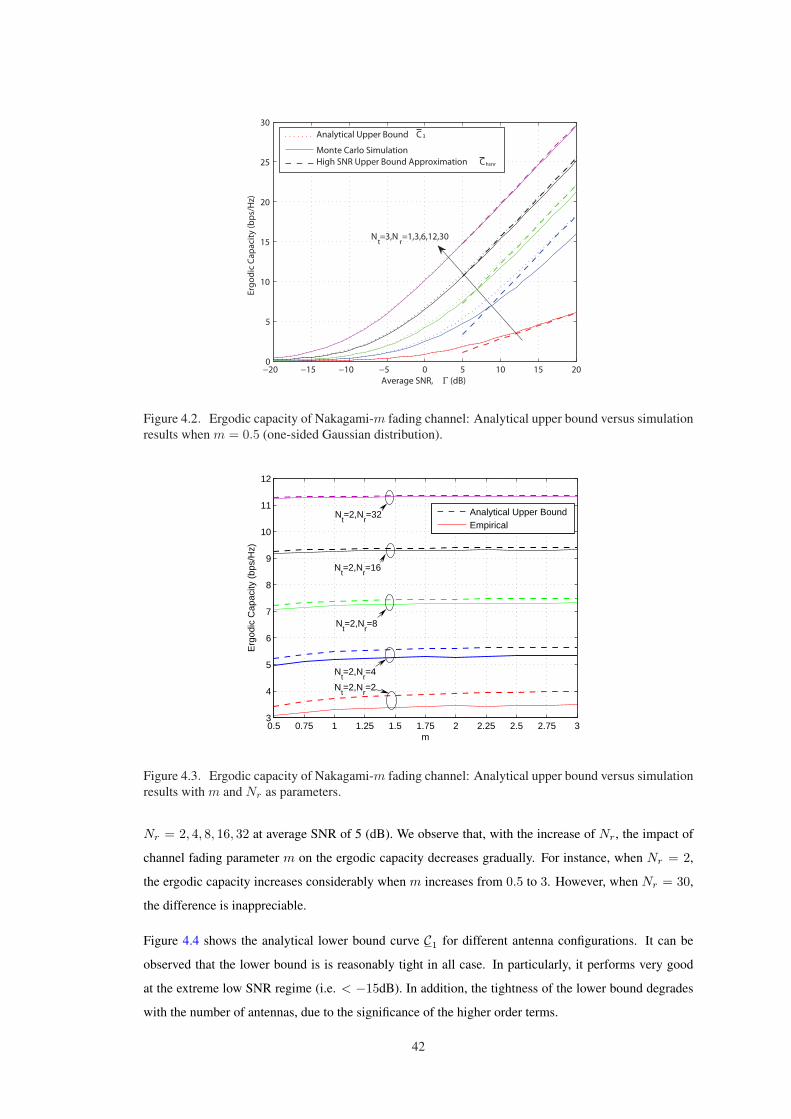
−20 −15 −10 −5 0 5 10 15 200

5

10

15

20

25

30

Average SNR, Γ (dB)

Erg

od

ic C

ap

aci

ty (

bp

s/H

z)

Analytical Upper Bound C 3

Monte Carlo Simulation

High SNR Upper Bound Approximation Chsnr

Nt=3,N

r=1,3,6,12,30

Figure 4.2. Ergodic capacity of Nakagami-m fading channel: Analytical upper bound versus simulationresults when m = 0.5 (one-sided Gaussian distribution).

0.5 0.75 1 1.25 1.5 1.75 2 2.25 2.5 2.75 33

4

5

6

7

8

9

10

11

12

m

Erg

odic

Cap

acity

(bp

s/H

z)

Analytical Upper BoundEmpirical

Nt=2,N

r=2

Nt=2,N

r=4

Nt=2,N

r=8

Nt=2,N

r=16

Nt=2,N

r=32

Figure 4.3. Ergodic capacity of Nakagami-m fading channel: Analytical upper bound versus simulationresults with m and Nr as parameters.

Nr = 2, 4, 8, 16, 32 at average SNR of 5 (dB). We observe that, with the increase of Nr, the impact of

channel fading parameter m on the ergodic capacity decreases gradually. For instance, when Nr = 2,

the ergodic capacity increases considerably when m increases from 0.5 to 3. However, when Nr = 30,

the difference is inappreciable.

Figure 4.4 shows the analytical lower bound curve C1 for different antenna configurations. It can be

observed that the lower bound is is reasonably tight in all case. In particularly, it performs very good

at the extreme low SNR regime (i.e. < −15dB). In addition, the tightness of the lower bound degrades

with the number of antennas, due to the significance of the higher order terms.

42

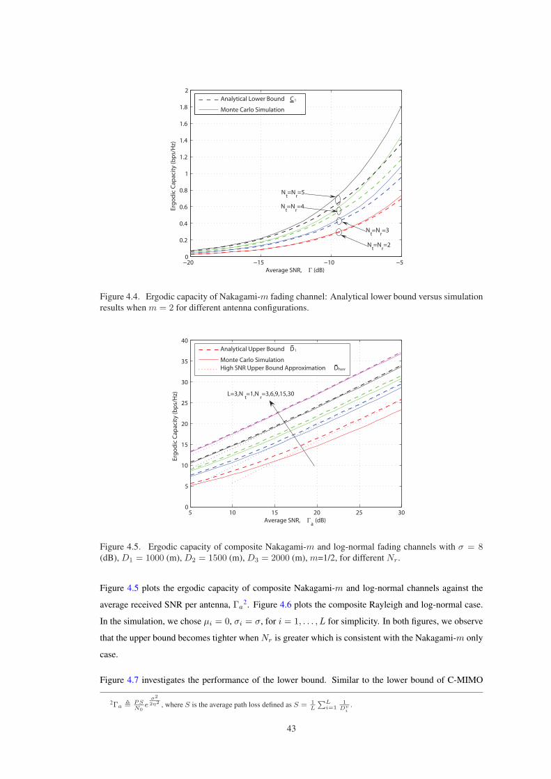
−20 −15 −10 −50

0.2

0.4

0.6

0.8

1

1.2

1.4

1.6

1.8

2

Average SNR, Γ (dB)

Erg

od

ic C

ap

aci

ty (

bp

s/H

z)

Analytical Lower Bound C1

Monte Carlo Simulation

Nt=N

r=5

Nt=N

r=4

Nt=N

r=3

Nt=N

r=2

Figure 4.4. Ergodic capacity of Nakagami-m fading channel: Analytical lower bound versus simulationresults when m = 2 for different antenna configurations.

5 10 15 20 25 300

5

10

15

20

25

30

35

40

Average SNR, Γa

(dB)

Erg

od

ic C

ap

aci

ty (

bp

s/H

z)

Analytical Upper Bound D1

Monte Carlo Simulation

High SNR Upper Bound Approximation Dhsnr

L=3,Nt=1,N

r=3,6,9,15,30

Figure 4.5. Ergodic capacity of composite Nakagami-m and log-normal fading channels with σ = 8(dB), D1 = 1000 (m), D2 = 1500 (m), D3 = 2000 (m), m=1/2, for different Nr.

Figure 4.5 plots the ergodic capacity of composite Nakagami-m and log-normal channels against the

average received SNR per antenna, Γa2. Figure 4.6 plots the composite Rayleigh and log-normal case.

In the simulation, we chose µi = 0, σi = σ, for i = 1, . . . , L for simplicity. In both figures, we observe

that the upper bound becomes tighter when Nr is greater which is consistent with the Nakagami-m only

case.

Figure 4.7 investigates the performance of the lower bound. Similar to the lower bound of C-MIMO

2Γa , PSN0

eσ2

2η2 , where S is the average path loss defined as S = 1L

PLi=1

1Dv

i.

43

−20 −10 0 10 20 300

5

10

15

20

25

30

Average SNR, Γa

(dB)

Erg

od

ic C

ap

aci

ty (

bp

s/H

z)

Analytical Upper Bound D2

Monte Carlo Simulation

High SNR Upper Bound Approximation Dhsnr

L=3,Nt=1,N

r=3,6,9,15,30

Figure 4.6. Ergodic capacity of composite Rayleigh and log-normal fading channels with σ = 8 (dB),D1 = 1000 (m), D2 = 1500 (m), D3 = 2000 (m), for different Nr.

channels, results illustrate that the lower bound is tight at low SNRs while it becomes looser at high

SNRs, particularly when the number of antennas increases.

−20 −15 −10 −5 00

0.2

0.4

0.6

0.8

1

1.2

1.4

1.6

1.8

2

Average SNR, Γa

(dB)

Erg

od

ic C

ap

aci

ty (

bp

s/H

z)

Analytical Lower Bound D2

Monte Carlo Simulation

Nt=N

r=1,2,3,4

Figure 4.7. Ergodic capacity of composite Rayleigh and log-normal fading channels: Analytical lowerbound versus simulation results when L = 1, σ = 8 (dB), D = 1000 (m), for different Nt, Nr.

4.6 Conclusion

In this chapter, by virtue of majorization theory, we have derived ergodic capacity bounds for C-MIMO

and D-MIMO fading channels. In C-MIMO, the capacity for Nakagami-m fading channels was inves-

tigated in detail, where we derived several tight upper bounds in terms of Meijer G-function, and in the

44

high SNR regime, a simple closed-form upper bound was presented to gain insight on the impacts of the

system parameters, such as fading severity m, the number of antennas Nt and Nr, etc. We also derived a

tight capacity lower bound for the low SNR regime. The same capacity analysis was also performed for

D-MIMO channels undergoing the composite (long-term) log-normal and (short-term) Nakagami fading

where similar upper and lower bounds were derived.

45

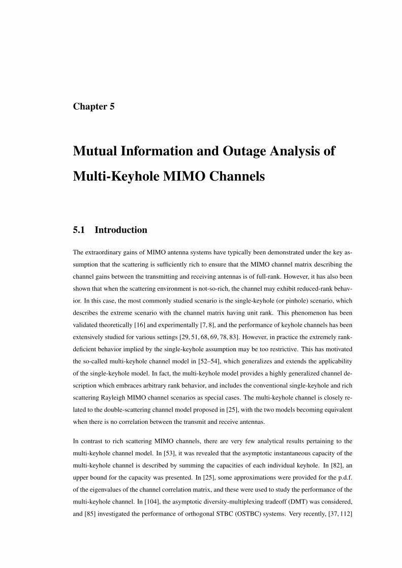
Chapter 5

Mutual Information and Outage Analysis of

Multi-Keyhole MIMO Channels

5.1 Introduction

The extraordinary gains of MIMO antenna systems have typically been demonstrated under the key as-

sumption that the scattering is sufficiently rich to ensure that the MIMO channel matrix describing the

channel gains between the transmitting and receiving antennas is of full-rank. However, it has also been

shown that when the scattering environment is not-so-rich, the channel may exhibit reduced-rank behav-

ior. In this case, the most commonly studied scenario is the single-keyhole (or pinhole) scenario, which

describes the extreme scenario with the channel matrix having unit rank. This phenomenon has been

validated theoretically [16] and experimentally [7, 8], and the performance of keyhole channels has been

extensively studied for various settings [29, 51, 68, 69, 78, 83]. However, in practice the extremely rank-

deficient behavior implied by the single-keyhole assumption may be too restrictive. This has motivated

the so-called multi-keyhole channel model in [52–54], which generalizes and extends the applicability

of the single-keyhole model. In fact, the multi-keyhole model provides a highly generalized channel de-

scription which embraces arbitrary rank behavior, and includes the conventional single-keyhole and rich

scattering Rayleigh MIMO channel scenarios as special cases. The multi-keyhole channel is closely re-

lated to the double-scattering channel model proposed in [25], with the two models becoming equivalent

when there is no correlation between the transmit and receive antennas.

In contrast to rich scattering MIMO channels, there are very few analytical results pertaining to the

multi-keyhole channel model. In [53], it was revealed that the asymptotic instantaneous capacity of the

multi-keyhole channel is described by summing the capacities of each individual keyhole. In [82], an

upper bound for the capacity was presented. In [25], some approximations were provided for the p.d.f.

of the eigenvalues of the channel correlation matrix, and these were used to study the performance of the

multi-keyhole channel. In [104], the asymptotic diversity-multiplexing tradeoff (DMT) was considered,

and [85] investigated the performance of orthogonal STBC (OSTBC) systems. Very recently, [37, 112]

studied the performance of MIMO multi-keyhole systems with CSIT, considering the special case of the

multi-keyhole channel for which the power of each keyhole is unity.

In this chapter, we present a thorough investigation of multi-keyhole MIMO channels. Based on some

newly derived statistical expressions for a product of complex random matrices presented in Chapter 3,

we examine the mutual information and outage performance of MIMO systems operating over multi-

keyhole channels. We consider two important scenarios. First, we derive new exact closed-form ex-

pressions and simplified upper and lower bounds for the ergodic mutual information, assuming that the

transmitter has no access to the CSI but the receiver has perfect knowledge. We then present new per-

formance results for optimal transmit beamforming scheme assuming both the transmitter and receiver

have perfect CSI.

5.2 System Model

We consider a communication link with Nt transmit and Nr receive antennas operating in frequency

non-selective channels. The received signals can be expressed in vector form as

y = Hx + n, (5.1)

where n ∼ CN (0, σ2I), and x = [x1, x2, . . . , xNt]T is the transmit symbol vector, with Ex‖x‖2 = P .

The matrix H represents the MIMO channel, which we model according to the multiple keyhole structure

as follows [53, 54]

H =Nk∑

k=1

akhr,kh†t,k = HrAH†

t , (5.2)

where Hr = [hr,1, . . . ,hr,Nk], Ht = [ht,1, . . . ,ht,Nk

], and A = diag(a1, . . . , aNk), with Nk de-

noting the total number of independent keyholes, and ak representing the complex gain for the kth

keyhole. Moreover, Hr and Ht are mutually-independent matrices ∼ CNNr,Nk(0Nr×Nk

, I ⊗ I) and

∼ CNNt,Nk(0Nt×Nk

, I ⊗ I), respectively. Let B ∆= AA†, We assume that channel is normalized such

that Etrace(HH†) = NrNt, and therefore trace(B) = 1.

For a general multi-keyhole MIMO channel, when the transmitter has no access to CSI while the receiver

has perfect knowledge, the ergodic mutual information of a MIMO multi-keyhole channel is readily

given by

I(γ) = EHr,Ht

log2 det

(I +

γ

NtH†H

), (5.3)

where γ , Pσ2 is the SNR per transmit antenna.

For transmit beamforming system, the transmitted signal vector is x = woptx, with x representing

the information symbol, and wopt denoting the optimal transmit weight vector given by the dominant

eigenvector of H†H (i.e., the eigenvector corresponding to the maximum eigenvalue). At the receiver,

the signals on each receive antenna are linearly combined according to the MRC principle using the

47

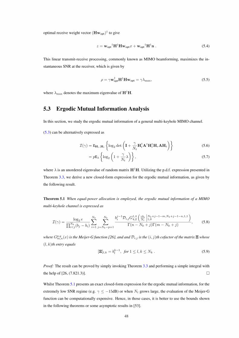
optimal receive weight vector (Hwopt)† to give

z = wopt†H†Hwoptx + wopt

†H†n . (5.4)

This linear transmit-receive processing, commonly known as MIMO beamforming, maximizes the in-

stantaneous SNR at the receiver, which is given by

ρ = γw†optH

†Hwopt = γλmax, (5.5)

where λmax denotes the maximum eigenvalue of H†H.

5.3 Ergodic Mutual Information Analysis

In this section, we study the ergodic mutual information of a general multi-keyhole MIMO channel.

(5.3) can be alternatively expressed as

I(γ) = EHr,Ht

log2 det

(I +

γ

NtH†

tA†H†

rHrAHt

)(5.6)

= pEλ

log2

(1 +

γ

Ntλ

), (5.7)

where λ is an unordered eigenvalue of random matrix H†H. Utilizing the p.d.f. expression presented in

Theorem 3.3, we derive a new closed-form expression for the ergodic mutual information, as given by

the following result.

Theorem 5.1 When equal-power allocation is employed, the ergodic mutual information of a MIMO

multi-keyhole channel is expressed as

I(γ) =log2 e∏Nk

i<j(bj − bi)

Nk∑

i=1

Nk∑

j=Nk−p+1

bj−1i Di,jG

1,44,2

(γbi

Nt

∣∣∣Nk+j−1−m,Nk+j−1−n,1,11,0

)

Γ(n−Nk + j)Γ(m−Nk + j), (5.8)

where Gp,qm,n(x) is the Meijer-G function [26], and andDi,j is the (i, j)th cofactor of the matrix Ξ whose

(l, k)th entry equals

[Ξ]l,k = bk−1l , for 1 ≤ l, k ≤ Nk . (5.9)

Proof: The result can be proved by simply invoking Theorem 3.3 and performing a simple integral with

the help of [26, (7.821.3)]. ¤

Whilst Theorem 5.1 presents an exact closed-form expression for the ergodic mutual information, for the

extremely low SNR regime (e.g. γ ≤ −15dB) or when Nt grows large, the evaluation of the Meijer-G

function can be computationally expensive. Hence, in those cases, it is better to use the bounds shown

in the following theorems or some asymptotic results in [53].

48

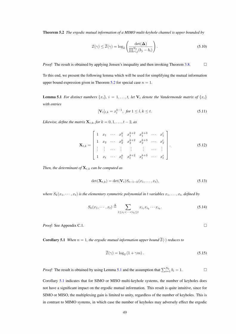
Theorem 5.2 The ergodic mutual information of a MIMO multi-keyhole channel is upper bounded by

I(γ) ≤ I(γ) = log2

(det(∆)∏Nk

i<j(bj − bi)

). (5.10)

Proof: The result is obtained by applying Jensen’s inequality and then invoking Theorem 3.8. ¤

To this end, we present the following lemma which will be used for simplifying the mutual information

upper bound expression given in Theorem 5.2 for special case n = 1.

Lemma 5.1 For distinct numbers xi, i = 1, . . . , t, let Vt denote the Vandermonde matrix of xiwith entries

[Vt]l,k = xk−1l , for 1 ≤ l, k ≤ t. (5.11)

Likewise, define the matrix Xt,k, for k = 0, 1, . . . , t− 2, as

Xt,k =

1 x1 · · · xk1 xk+2

1 xk+31 · · · xt

1

1 x2 · · · xk2 xk+2

2 xk+32 · · · xt

2

...... · · · ...

...... · · · ...

1 xt · · · xkt xk+2

t xk+3t · · · xt

t

. (5.12)

Then, the determinant of Xt,k can be computed as

det(Xt,k) = det(Vt)St−1−k(x1, . . . , xt), (5.13)

where Sk(x1, · · · , xt) is the elementary symmetric polynomial in t variables x1, . . . , xt, defined by

Sk(x1, · · · , xt)∆=

∑

1≤i1<···<ik≤t

xi1xi2 · · ·xik. (5.14)

Proof: See Appendix C.1. ¤

Corollary 5.1 When n = 1, the ergodic mutual information upper bound I(·) reduces to

I(γ) = log2 (1 + γm) . (5.15)

Proof: The result is obtained by using Lemma 5.1 and the assumption that∑Nk

i=1 bi = 1. ¤

Corollary 5.1 indicates that for SIMO or MISO multi-keyhole systems, the number of keyholes does

not have a significant impact on the ergodic mutual information. This result is quite intuitive, since for

SIMO or MISO, the multiplexing gain is limited to unity, regardless of the number of keyholes. This is

in contrast to MIMO systems, in which case the number of keyholes may adversely effect the ergodic

49

mutual information. This effect is most significant when the number of keyholes is less than the number

of transmit and receive antennas, in which case the number of keyholes limits the multiplexing gain of

the system.

Theorem 5.3 The ergodic mutual information of a MIMO multi-keyhole channel is lower bounded by

I(γ) ≥ I(γ) =

p log2

(1 +

γ

Ntexp

(1p

[p∑

s=1

ψ(m− p + s) +p∑

s=1

ψ(n− p + s) +

∑Nk

s=Nk−p+1 det(Ys)∏Nk

i<j(bj − bi)

])),

(5.16)

where Ys has been defined in (3.63).

Proof: Utilizing the result in [72, Theorem 1] and Theorem 3.10 yields the desired result. ¤

Corollary 5.2 When p = 1, the ergodic mutual information lower bound I(·) reduces to

I(γ) = log2

(1 +

γ

Ntexp

(ψ(m) + ψ(n) +

det(YNk)∏Nk

i<j(bj − bi)

)). (5.17)

If p = Nk = 1, then

I(γ) = log2

(1 +

γ

Ntexp (ψ(m) + ψ(n))

). (5.18)

Proof: The proof is straightforward and is omitted. ¤

5.4 Outage Analysis of MIMO-MRC system

In this section, we analyze the outage performance of MIMO-MRC system in multi-keyhole MIMO

channels, which is defined as the probability that the received SNR drops below some predefined thresh-

old, i.e.,

Pout(γth)∆= Pr(ρ < γth) . (5.19)

From Equation (5.5), it is clear that the performance of this optimal MIMO beamforming system is

determined by the statistics of λmax. Invoking Theorem 3.3, we obtain the following result

Theorem 5.4 The outage probability of the optimal MIMO beamforming system in multi-keyhole chan-

nels can be expressed as

Pout(γth) =(−1)

p(p−1)2 det

(Φ

(γth

γ

))

∏pi=1 Γ(n− i + 1)

∏Nk

i<j(bj − bi), (5.20)

50

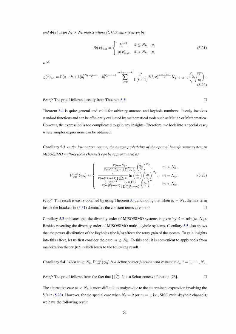
and Φ(x) is an Nk ×Nk matrix whose (l, k)th entry is given by

[Φ(x)]l,k =

bk−1l , k ≤ Nk − p,

g(x)l,k, k > Nk − p,(5.21)

with

g(x)l,k = Γ(q − k + 1)b2Nk−p−kl − bNk−n−1

l

m+q−n−k∑t=0

xt

Γ(t + 1)2(blx)

q−t−k+12 Kq−t−k+1

(2√

x

bl

).

(5.22)

Proof: The proof follows directly from Thoerem 3.3. ¤

Theorem 5.4 is quite general and valid for arbitrary antenna and keyhole numbers. It only involves

standard functions and can be efficiently evaluated by mathematical tools such as Matlab or Mathematica.

However, the expression is too complicated to gain any insights. Therefore, we look into a special case,

where simpler expressions can be obtained.

Corollary 5.3 In the low outage regime, the outage probability of the optimal beamforming system in

MISO/SIMO multi-keyhole channels can be approximated as

Pn=1out (γth) ≈

Γ(m−Nk)

Γ(m)Γ(Nk+1)QNk

i=1 bi

(γth

γ

)Nk

, m > Nk,

1

Γ(m)Γ(m+1)QNk

i=1 bi

ln(

γγth

)(γth

γ

)Nk

, m = Nk,

(−1)m−1

Γ(m)Γ(m+1)det(Φ4)QNki<j(bj−bi)

(γth

γ

)m

, m < Nk.

(5.23)

Proof: This result is easily obtained by using Theorem 3.4, and noting that when m = Nk, the lnx term

inside the brackets in (3.31) dominates the constant terms as x → 0. ¤

Corollary 5.3 indicates that the diversity order of MISO/SIMO systems is given by d = min(m,Nk).

Besides revealing the diversity order of MISO/SIMO multi-keyhole systems, Corollary 5.3 also shows

that the power distribution of the keyholes (the bi’s) affects the array gain of the system. To gain insights

into this effect, let us first consider the case m ≥ Nk. To this end, it is convenient to apply tools from

majorization theory [62], which leads to the following result.

Corollary 5.4 When m ≥ Nk, Pn=1out (γth) is a Schur-convex function with respect to bi, i = 1, · · · , Nk.

Proof: The proof follows from the fact that∏Nk

i=1 bi is a Schur-concave function [73]. ¤

The alternative case m < Nk is more difficult to analyze due to the determinant expression involving the

bi’s in (5.23). However, for the special case when Nk = 2 (or m = 1, i.e., SISO multi-keyhole channel),

we have the following result.

51

Table 5.1. Power distribution among keyholes.

Nk (b1, . . . , bNk)

1 (1)2 (0.4, 0.6)3 (0.2, 0.3, 0.5)4 (0.1, 0.2, 0.3, 0.4)5 (0.05, 0.1, 0.2, 0.3, 0.35)6 (0.05, 0.1, 0.12, 0.13, 0.25, 0.35)

Corollary 5.5 When Nk = 2 and m = 1, Pn=1out (γth) is a Schur-convex function with respect to bi, for

i = 1, . . . , Nk.

Proof: See Appendix C.2. ¤

Both Corollary 5.4 and Corollary 5.5 indicate that as the power distribution amongst the keyholes (i.e.,

the bi’s) becomes “less spread”, the outage probability improves.

5.5 Numerical Results

In this section, we provide some numerical results to verify the analytical expressions derived in the

above sections. In all simulations, the power distribution among keyholes is given in Table 5.1, and the

simulation results are obtained based on 100,000 independent channel realizations.

Figure 5.1 plots the exact curve according to (5.8) against Monte-Carlo simulation curves for Nt = 5,

Nr = 3 with different Nk. As observed from Figure 5.1, the analytical curves match perfectly with

the Monte-Carlo simulation curves for all cases, which confirms the correctness of the analytical results.

It is also observed that the mutual information of multi-keyhole channel is always inferior to that of a

standard MIMO channel with same Nt and Nr.

Figure 5.2 compares the ergodic mutual information upper (5.10) and lower bound (5.16) with the exact

results in (5.8). We see that both bounds are very tight. Moreover, in the low SNR regime the upper

bound and exact results coincide, whilst in the high SNR regime the lower bound and exact results

coincide.

Figure 5.3 illustrates the outage probability for the optimal MIMO beamforming system in multi-keyhole

channels. We see that when the number of keyholes increases, the performance approaches that of a

Rayleigh MIMO channel. Surprisingly, we also observe that there is a crossover point, indicating that at

high outage levels (equivalently, at sufficiently low SNR), the performance of a multi-keyhole channel

can be superior than that of a Rayleigh MIMO channel. However, despite this cross-over point, for

outage levels of practical interest (eg. < 0.1), achieving a given outage level requires lower SNR for a

Rayleigh MIMO channel compared with multi-keyhole channels.

52

0 5 10 15 202

4

6

8

10

12

14

16

18

20

P/σ2 (dB)

Erg

odic

Cap

acity

(bp

s/H

z)

MIMO Rayleigh Nt=5,N

r=3

Analytical Nt=5,N

r=3,N

k=2

Analytical Nt=5,N

r=3,N

k=4

Analytical Nt=5,N

r=3,N

k=6

Monte Carlo

Figure 5.1. Ergodic mutual information of multi-keyhole MIMO channels with equal-power allocation.

0 5 10 15 20 25 300

5

10

15

20

25

30

P/σ2 (dB)

Erg

odic

Cap

acity

(bp

s/H

z)

Monte CarloExact AnalyticalUpper boundLower bound

(Nt=3,N

r=5,N

k=6)

(Nt=5,N

r=3,N

k=2)

Figure 5.2. Ergodic mutual information bounds for MIMO multi-keyhole channels.

Figure 5.4 compares the exact outage probability curves based on Theorem 5.4, low outage approxima-

tion curves based on Corollary 5.3, and Monte-Carlo simulated curves. Results are shown for a system

with Nt = 4, Nr = 1, and different numbers of keyholes. It can be observed that the approximation

curves are very accurate in the low outage regime. We also see that the slope of the outage curves are

determined by the minimum of Nk and m; thereby confirming our diversity analysis.

Figure 5.5 illustrates the impact of the power distribution on the outage curves when Nt = 4, Nr = 1,

and Nk = 2. Three curves are plotted according to the power distributions (b1, b2) corresponding to

(0.05, 0.95), (0.15, 0.85) and (0.45, 0.55), respectively. Note that

(0.05, 0.95) Â (0.15, 0.85) Â (0.45, 0.55), (5.24)

53

−15 −10 −5 0 510

−7

10−6

10−5

10−4

10−3

10−2

10−1

100

P/σ2

Out

age

Pro

babi

lity

MIMO Rayleigh Nt=5,N

r=3

Analytical Nt=5,N

r=3,N

k=2

Analytical Nt=5,N

r=3,N

k=4

Analytical Nt=5,N

r=3,N

k=6

Monte Carlo

Figure 5.3. The outage probability of the optimal MIMO beamforming system in multi-keyhole chan-nels.

−5 0 5 10 15 2010

−7

10−6

10−5

10−4

10−3

10−2

10−1

100

P/σ2

Out

age

Pro

babi

lity

AnalyticalApproximationMonte Carlo

(4,1,6)

(4,1,4)

(4,1,2)

Figure 5.4. The outage probability of the optimal beamforming system in MISO multi-keyhole channelsfor different number of keyholes with Nt = 4, Nr = 1.

which, from Corollary 5.4, implies that

Pn=1out (γth)(0.05,0.95) ≥ Pn=1

out (γth)(0.15,0.85) ≥ Pn=1out (γth)(0.45,0.55) . (5.25)

The outage curves in Figure 5.5 confirm this analysis.

5.6 Conclusion

Multi-keyhole MIMO channels bridge the gap between single-keyhole and rich-scattering (full-rank)

MIMO channels. In this chapter, we have provided an analytical characterization of the statistical prop-

54

−5 0 5 10 15 20

10−4

10−3

10−2

10−1

100

P/σ2

Out

age

Pro

babi

lity

AnalyticalApproximationMonte Carlo

(0.45,0.55)

(0.15,0.85)

(0.05,0.95)

Figure 5.5. The outage probability of the optimal beamforming system in MISO multi-keyhole channelswith different power distributions with Nt = 4, Nr = 1, Nk = 2.

erties of multi-keyhole MIMO channel matrices. In particular, we derived exact expressions for the p.d.f.

of an unordered eigenvalue, exact and asymptotic expressions for the distribution of the maximum eigen-

value, as well as closed-form expressions for the expected log-determinant and expected characteristic

polynomial. These results were applied to investigate the ergodic MIMO mutual information, and the

outage probability of optimal transmit beamforming in multi-keyhole MIMO channels. The findings

suggest that performance in multi-keyhole MIMO channels is generally inferior to that of rich-scattering

MIMO channels.

55

Chapter 6

Capacity of AF MIMO Dual-Hop Systems

6.1 Introduction

Point-to-point MIMO communication systems have been receiving considerable attention in the last

decade due to their potential for providing linear capacity growth and significant performance improve-

ments over conventional SISO systems [23, 94]. Recently, the application of MIMO techniques in a

cooperative communication setting [49, 50, 79, 80] has become a topic of increasing interest as a means

of achieving further performance improvements in wireless networks [12, 13, 70, 99, 101].

A great deal of research works has been conducted to gain fundamental understanding of the capac-

ity of this class of systems [11, 65, 66, 97, 98, 105]. In [11], the ergodic capacity of AF MIMO dual-

hop systems was examined for a large numbers of relay antennas K, and was shown to scale with

log K. Asymptotic ergodic capacity results were also obtained in [97] by means of the replica method

from statistical physics. In [65, 66], the asymptotic network capacity was examined as the number of

source/desination antennas M and relay antennas K grew large with a fixed-ratio K/M → β using

tools from large-dimensional RMT. It was demonstrated that for β → ∞, the relay network behaved

equivalently to a point-to-point MIMO link. The results of [65, 66] were further elaborated in [105]

where a general asymptotic ergodic capacity formula was presented for multi-level AF relay networks.

Recently, the asymptotic mean and variance of the mutual information in correlated Rayleigh fading was

studied in [98].

All of these prior capacity results, however, were derived by employing asymptotic methods (i.e., by

letting the system dimensions grow to infinity). There appear to be no analytical ergodic capacity results

which apply for AF MIMO dual hop systems with arbitrary finite antenna and relaying configurations.

In this chapter we derive new exact analytical results, simple closed-form high SNR expressions, and

tight closed-form upper and lower bounds on the ergodic capacity of AF MIMO dual-hop systems. In

contrast to previous results, our expressions apply for any finite number of MIMO antennas and for

arbitrary number of relay antennas.

ns n nr

H1 H2

Source Relay Destination

d

Figure 6.1. Schematic diagram of a MIMO dual-hop system, where there is no direct link betweensource and destination.

6.2 System Model

We employ the same AF MIMO dual-hop system model as in [65, 66]. In particular, suppose that there

are ns source antennas, nr relay antennas and nd destination antennas, which we represent by the 3-

tuple (ns, nr, nd). All terminals operate in half-duplex mode, and as such communication occurs from

source to relay and from relay to destination in two separate time slots. It is assumed that there is no

direct communication link between the source and destination, as sketched in Figure 6.1. The end-to-end

input-output relation of this channel is then given by

y = H2FH1s + H2Fnnr+ nnd

(6.1)

where s is the transmit symbol vector, nnr and nndare the relay and destination noise vectors respec-

tively, F =√

α/ (nr (1 + ρ))Inr (α corresponds to the overall power gain of the relay terminal) is the

forwarding matrix at the relay terminal which simply forwards scaled versions of its received signals,

and H1 ∼ CNnr,ns(0nr×ns

, I⊗ I) and H2 ∼ CNnd,nr(0nd×nr

, I⊗ I) denote the channel matrices of

the first hop and the second hop respectively. The input symbols are chosen to be i.i.d. zero-mean circu-

lant symmetric complex Gaussian (ZMCSCG) random variables and the per antenna power is assumed

to be ρ/ns, i.e., Ess†

= (ρ/ns) Ins

. The additive noise at the relay and destination are assumed to be

white in both space and time and are modeled as ZMCSCG with unit variance, i.e., Ennr

n†nr

= Inr

and Ennd

n†nd

= Ind

. We assume that the source and relay have no CSI, and that the destination has

perfect knowledge of both H2 and H2H1.

The ergodic capacity (in b/s/Hz) of the AF MIMO dual-hop system described above can be written

as [65, 66, 97]

C =12E

log2 det

(I + RsR−1

n

)(6.2)

57

where Rs and Rn are nd × nd matrices given by

Rs =ρa

nsH2H1H

†1H

†2 (6.3)

and

Rn = Ind+ aH2H

†2 (6.4)

respectively, with

a =α

nr (1 + ρ). (6.5)

Using the identity

det (I + AB) = det (I + BA) , (6.6)

(6.2) can be alternatively expressed as

C (ρ) =12E

log2 det

(Ins

+ρa

nsH†

1H†2R

−1n H2H1

). (6.7)

Next, we utilize the singular value decomposition to write H2 = U2D2V†2, where

D2 = diagλ1, . . . , λmin(nd,nr)

(6.8)

is an nd × nr diagonal matrix, with diagonal elements pertaining to the increasing ordered singular

values, and U2 ∈ Cnd×nd and V2 ∈ Cnr×nr are unitary matrices containing the respective eigenvectors.

Since H1 is invariant under left and right unitary transformation, the ergodic capacity in (6.7) can be

further simplified as

C (ρ) =12E

log2 det

(Inr

+ρa

nsH†

1ΨH1

), (6.9)

where

Ψ =

diag

λ21

1+aλ21, . . . ,

λ2nr

1+aλ2nr

, nr ≤ nd,

diag

λ21

1+aλ21, . . . ,

λ2nd

1+aλ2nd

, 0, . . . , 0︸ ︷︷ ︸nr−nd

, nr > nd.

(6.10)

It is then easily established that

C (ρ) =12E

log2 det

(Ins

+ρa

nsH†

1LH1

), (6.11)

58

where H†1 ∼ CNns,q (0, Ins ⊗ Iq), with q = min (nd, nr), and

L = diagλ2

i /(1 + aλ2

i

)q

i=1. (6.12)

Equivalently, we can now write

C (ρ) =s

2

∫ ∞

0

log2

(1 +

ρa

nsλ

)fλ (λ) dλ, (6.13)

where s = min (ns, q), λ denotes an unordered eigenvalue of the random matrix H†1LH1, and fλ (·)

denotes the corresponding p.d.f..

6.3 Exact Ergodic Capacity Analysis

In this section, we present new analytical expressions for the ergodic capacity of AF MIMO dual-hop

systems.

Theorem 6.1 The exact ergodic capacity of AF MIMO dual-hop systems can be expressed as

C (ρ) = Kq∑

l=1

q∑

k=q−s+1

q+ns−l∑

i=0

(q+ns−l

i

)aq+ns−l−i

Γ (ns − q + k)Gl,kJi,k, (6.14)

where

K =(∏q

i=1Γ (q − i + 1)Γ (p− i + 1)

)−1

, (6.15)

and

Ji,k =∫ ∞

0

log2

(1 +

ρa

nsλ

)e−λaλ(2ns+2k+p−q−i−3)/2Kp+q−i−1

(2√

λ)

dλ . (6.16)

Proof: The above result can be obtained by substituting the p.d.f. expression of an unordered eigenvalue

derived in Theorem 3.1 in (6.13). ¤

The integral in (6.16) can be evaluated either numerically, or can be expressed as an infinite series

involving Meijer-G functions. To this end, we examine the ergodic capacity relationship of AF MIMO

dual-hop systems and single-hop MIMO systems in the following subsection.

6.3.1 Analogies with Single-Hop MIMO Ergodic Capacity

Let CSH−MIMO(ns, nd, ρ) denote the ergodic capacity of a conventional single-hop i.i.d. Rayleigh fading

MIMO channel matrix H ∼ CNnd,ns(0nd×ns , I ⊗ I), with ns transmit and nd receive antennas, and

59

average SNR ρ, i.e..

CSH−MIMO(ns, nd, ρ) = E

log2 det

(Ind

+ρ

nsHH†

). (6.17)

Here, we demonstrate four particular cases for which the AF MIMO dual-hop channel relates directly to

single-hop MIMO channels, in terms of ergodic capacity.

• As the number of relay antennas grows large, i.e., nr → ∞, the ergodic capacity of AF MIMO

dual-hop systems becomes

limnr→∞

C (ρ) =12CSH−MIMO

(ns, nd,

ρα

1 + ρ + α

). (6.18)

A proof is presented in Appendix D.1. Note that a similar phenomenon has been derived in [11],

for the special case ns = nd. Here, (6.18) generalizes that result for arbitrary source and destina-

tion antenna configurations.

• As the number of source antennas grows large, i.e., ns → ∞, the ergodic capacity of AF MIMO

dual-hop systems becomes

limns→∞

C (ρ) =12CSH−MIMO (nr, nd, α)− 1

2CSH−MIMO

(nr, nd,

α

1 + ρ

). (6.19)

A proof is presented in Appendix D.2. Interestingly, we see that as ρ grows large, the right-most

term in (6.19) disappears, and the AF MIMO dual-hop capacity becomes equivalent to one half

of the ergodic capacity of a single-hop MIMO channel with nr transmit antennas, nd receive

antennas, and average SNR α.

• As the number of destination antennas grows large, i.e., nd → ∞, the ergodic capacity of AF

MIMO dual-hop systems becomes

limnd→∞

C (ρ) =12CSH−MIMO (ns, nr, ρ) . (6.20)

The result is trivially obtained by directly taking λ2i → ∞ in (6.11). We see that the AF MIMO

dual-hop capacity becomes equivalent to one half of the ergodic capacity of a single-hop MIMO

channel with ns transmit antennas, nr receive antennas, and average SNR ρ.

• As the power gain of the relay grows large, i.e., α → ∞, the ergodic capacity of AF MIMO

dual-hop systems becomes

limα→∞

C (ρ) =12CSH−MIMO (ns, q, ρ) . (6.21)

The result is trivially obtained by directly taking α → ∞ in (6.11). Thus we see the interesting

result that even as the relay power gain becomes very large, the capacity of AF MIMO dual-hop

60

channels remains bounded, and in fact becomes equivalent to one half of the ergodic capacity of

a single-hop MIMO channel with ns transmit antennas, q = min(nr, nd) receive antennas, and

average SNR ρ.

We note that for each of the cases (6.18)–(6.21), closed-form expressions can be obtained by directly

invoking known results from the single-hop MIMO capacity literature (eg. see [82]).

In order to obtain further simplified closed-form results, it is useful to investigate the ergodic capacity in

the high SNR regime. This is presented in the subsection below.

6.3.2 High SNR Capacity Analysis

For the high SNR regime, we consider one important scenario where the source and relay powers grow

large proportionately.

Here we have α → ∞, ρ → ∞, with α/ρ = β, for some fixed β. Then ρa → αnr

and a → β/nr, and

the ergodic capacity at high SNR reduces to

C (ρ)|α,ρ→∞,α/ρ=β =12E

log2 det

(Ins

+ρβ

nsnrH†

1LH1

), (6.22)

where L = diagλ2

i /(1 + (β/nr) λ2

i

)q

i=1. We can express (6.22) in the general form [57]

C (ρ)|α,ρ→∞,,α/ρ=β = S∞

(ρ|dB

3dB− L∞

)+ o (1) , (6.23)

where 3dB = 10 log10(2). Here, the two key parameters are S∞, which denotes the high-SNR slope in

bits/s/Hz/(3 dB) given by

S∞ = limα,ρ→∞

C (ρ)|α,ρ→∞,α/ρ=β

log2(ρ)(6.24)

and L∞, which represents the high-SNR power offset in 3 dB units given by

L∞ = limα,ρ→∞

(log2(ρ)−

C (ρ)|α,ρ→∞,α/ρ=β

S∞

). (6.25)

From (6.22), we can evaluate S∞ and L∞ in closed-form as follows.

Theorem 6.2 For the case α → ∞, ρ → ∞, with α/ρ = β, the high-SNR slope and high-SNR power

offset of AF MIMO dual-hop systems are given by

S∞ =s

2bit/s/Hz/(3dB) (6.26)

61

and1

L∞(ns, nr, nd) = log2

(nsnr

β

)− 1

s ln 2

s∑

k=1

ψ (ns + k − s) +Kq∑

k=q−s+1

det(Wk

) (6.27)

respectively, where Wk is a q × q matrix with entries

Wk

m,n

=

(βnr

)1−τ

ϑτ−1

(βnr

), n 6= k,

ςm+n

(βnr

), n = k.

(6.28)

For the case q = s (i.e. corresponding to min(ns, nr, nd) = nd or min(ns, nr, nd) = nr), the high SNR

power offset (6.27) admits the alternative form

L∞(ns, nr, nd) = log2

(nsnr

β

)− 1

s ln 2

s∑

k=1

ψ (ns − s + k) +q−1∑

i=0

i∑

j=0

2j∑

l=0

2q−l−2∑

k=0

(2q − l − 2

k

)

×A (i, j, l, p, q)(

β

nr

)2q−l−2−k

Γ (p + q − k − 1)

(ψ (p + q − k − 1)−

p+q−k−2∑m=0

gm

(nr

β

))].

(6.29)

Proof: See Appendix D.3. ¤

Interestingly, we see that the high SNR slope depends only on the minimum system dimension, i.e.

s = min(ns, nr, nd), whereas the high SNR power offset is a much more intricate function of ns, nr,

and nd.

It is important to note that Theorem 6.2 presents an exact characterization of the key high SNR ergodic

capacity parameters, S∞ and L∞(·), for arbitrary numbers of antennas at the source, relay, and desti-

nation terminals. We now examine some particular cases of Theorem 6.2, in which these expressions

reduce to simple forms.

Corollary 6.1 Let nr = 1. Then S∞ = 1/2, and L∞(·) reduces to

L∞(ns, 1, nd) = log2

(ns

β

)− 1

ln 2

[ψ (ns) + ψ (nd)−

nd−1∑m=0

gm

(1β

)]. (6.30)

Note that, as ns grows large, ψ (ns) = lnns + o(1) [4, (6.3.18)], where the o(1) term disappears as

ns →∞, and as such we have

limns→∞

L∞(ns, 1, nd) = log2

(1β

)− 1

ln 2

[ψ (nd)−

nd−1∑m=0

gm

(1β

)]. (6.31)

1Note that here we explicitly indicate the dependence of the high SNR power offset on ns, nr , and nd.

62

Corollary 6.2 Let nd = 1. Then S∞ = 1/2, and L∞(·) reduces to

L∞(ns, nr, 1) = log2

(nsnr

β

)− 1

ln 2

[ψ (ns) + ψ (nr)−

nr−1∑m=0

gm

(nr

β

)]. (6.32)

In this case, as ns grows large we have

limns→∞

L∞(ns, nr, 1) = log2

(nr

β

)− 1

ln 2

[ψ (nr)−

nr−1∑m=0

gm

(nr

β

)]. (6.33)

Based on these results, we can easily examine the effect of the relative power gain factor β on the

ergodic capacity. In particular, noting that gl (x) in (3.59) is a monotonically decreasing function of

x in the interval2 [0,∞), we see that increasing β, whilst having no effect on the high SNR capacity

slope S∞, results in decreasing the high SNR power offset L∞(·), and therefore increasing the ergodic

capacity in the high SNR regime.

Corollary 6.3 Let ns = nr = 1. Adding k destination antennas, while not altering S∞, would reduce

the high SNR power offset as

δ(nd, k) ∆= L∞ (1, 1, nd + k)− L∞ (1, 1, nd)

= − 1ln 2

nd+k−1∑

l=nd

(1`

+ gl

(1β

)). (6.34)

Note that, to obtain this result, we have invoked the definition of the digamma function [26]. Since

gl (x) > 0 for x ∈ [0,∞), it is clear that the high SNR power offset L∞(·) in (6.34) is a decreas-

ing function of k, thereby confirming the intuitive notion that adding more antennas to the destination

terminal has the effect of improving the ergodic capacity.

6.4 Ergodic Capacity Upper Bound

The following theorem presents a new tight upper bound on the ergodic capacity of AF MIMO dual-hop

systems.

Theorem 6.3 The ergodic capacity of AF MIMO dual-hop systems is upper bounded by

C (ρ) ≤ CU (ρ) =12

log2

(K det(Ξ)), (6.35)

where Ξ is defined in (3.47).

2This conclusion is easily established by noting that d/dx (gl (x)) = ex [El+1 (x)− El (x)], and using [4, Eq. 5.1.17].

63

Proof: Application of Jensen’s inequality gives3

C (ρ) 6 12

log2 E

det

(Ins

+ρa

nsH†

1LH1

). (6.36)

The result now follows by using Theorem 3.7. ¤

The following corollaries present some example scenarios for which the upper bound (6.35) reduces to

simplified forms.

Corollary 6.4 For the case ns →∞, CU (ρ) becomes

limns→∞

CU (ρ) =12

log2

(Kdet(Ξ1)), (6.37)

where Ξ1 is a q × q matrix with entries

Ξ1

m,n

= a1−τϑτ−1(a) + ρa1−τϑτ (a). (6.38)

Proof: The proof is straightforward and is omitted. ¤

This result shows that in AF MIMO dual-hop systems, when the numbers of antennas at both the relay

and destination remain fixed, the ergodic capacity remains bounded as the number of source antennas

grows large. This is in agreement with the results in Section 6.3.1.

Note that for the scenarios nr → ∞ and nd → ∞, simplified closed-form results can also be obtained

by taking the corresponding limits in (6.37) or, alternatively, by using the equivalent single-hop MIMO

capacity relations in (6.18) and (6.20), and applying known upper bounds for single-hop MIMO channels

in [72]. We omit these expressions here for the sake of brevity.

Corollary 6.5 Let nr = 1. Then, CU (ρ) reduces to

Cnr=1U (ρ) =

12

log2

(1 + ρnde

1+ρα End+1

(1 + ρ

α

)). (6.39)

When nd →∞, Cnr=1U (ρ) becomes

limnd→∞

Cnr=1U (ρ) =

12

log2 (1 + ρ) . (6.40)

When α →∞, Cnr=1U (ρ) becomes

limα→∞

Cnr=1U (ρ) =

12

log2 (1 + ρ) . (6.41)

3Note that this inequality has also been applied in the ergodic capacity analysis of single-user single-hop MIMO systems (seeeg. [36, 63, 108]).

64

Proof: See Appendix D.4. ¤

This shows the interesting result that if a single relay antenna is employed, then when either the number

of destination antennas nd or the relay gain α grows large, the ergodic capacity is upper bounded by the

capacity of an AWGN SISO channel.

Corollary 6.6 In the high SNR regime, (i.e., as ρ →∞) for fixed relay gain α, CU (ρ) becomes

limρ→∞

CU (ρ) =12

log2

(K det(Ξ)

), (6.42)

where Ξ is a q × q matrix with entries

Ξ

m,n

=

Γ (τ − 1), n ≤ q − ns,

Γ (τ − 1)(1 + α

nsnr(ns − q + n) (τ − 1)

), n > q − ns.

(6.43)

Proof: The proof follows from the observation that when ρ → ∞, then a → 0, and that asymptotic

first-order expansion for confluent hypergeometric function U [4] can be expressed as

U (c, b, z) = z−c + o (1) , z →∞. (6.44)

¤

6.5 Ergodic Capacity Lower Bound

The following theorem presents a new tight lower bound on the ergodic capacity of AF MIMO dual-hop

systems.

Theorem 6.4 The ergodic capacity of AF MIMO dual-hop systems is lower bounded by

C (ρ) ≥ CL(ρ) =s

2log2

1 +

ρa

nsexp

1

s

s∑

k=1

ψ (ns − s + k) +Kq∑

k=q−s+1

det (Wk)

,

(6.45)

where Wk is defined as in (3.57).

Proof: See Appendix D.5. ¤

The following corollaries present some example scenarios for which the lower bound (6.45) reduces to

simplified forms.

65

Corollary 6.7 For the case ns →∞, CL(ρ) reduces to

limns→∞

CL (ρ) =s

2log2

(1 + ρa exp

(Ks

q∑

k=1

det (Wk)

)). (6.46)

Proof: When ns →∞, ψ (ns − q + k) can be approximated as [4, (6.3.18)]

ψ (ns − q + k)|ns→∞ ≈ ln (ns − q + k)

≈ lnns. (6.47)

Substituting (6.47) into (6.45) yields the desired result. ¤

Again, we note that for the scenarios nr →∞ and nd →∞, simplified closed-form results can also be

obtained by taking the corresponding limits in (6.37) or, alternatively, by using (6.18) and (6.20), and

applying known lower bounds for single-hop MIMO channels in [72].

Corollary 6.8 For the case nr = 1, CL(ρ) reduces to

Cnr=1L (ρ) =

12

log2

(1 +

ρα

ns (1 + ρ)exp

(ψ (ns) + ψ (nd)− e(1+ρ)/α

nd−1∑

l=0

El+1

(1 + ρ

α

))).

(6.48)

When ns →∞, Cnr=1L (ρ) becomes

limns→∞

Cnr=1L (ρ) =

12

log2

(1 +

ρα

1 + ρexp

(ψ (nd)− e(1+ρ)/α

nd−1∑

l=0

El+1

(1 + ρ

α

))). (6.49)

When nd →∞, Cnr=1L (ρ) becomes

limnd→∞

Cnr=1L (ρ) =

12

log2

(1 +

ρα

ns (1 + ρ)exp

(ψ (ns) + ψ

(1 + ρ

α

))). (6.50)

When α →∞, CL(ρ) becomes

limα→∞

Cnr=1L (ρ) =

12

log2

(1 +

ρ

nsexp (ψ (ns))

). (6.51)

Proof: See Appendix D.6. ¤

As also observed from the upper bound in Corollary 6.5, this result shows that for a system with a single

relay antenna, when the relay gain α grows large, the ergodic capacity of an AF MIMO dual-hop channel

is lower bounded by the capacity of an AWGN SISO channel (with scaled average SNR).

66

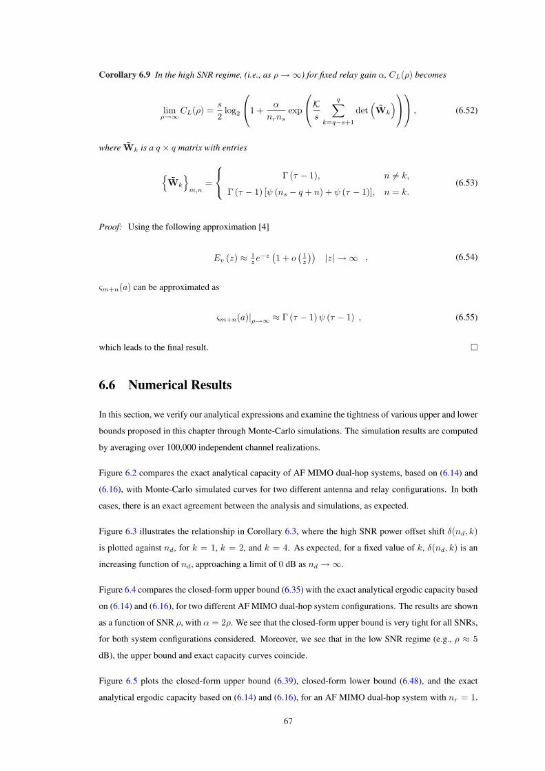
Corollary 6.9 In the high SNR regime, (i.e., as ρ →∞) for fixed relay gain α, CL(ρ) becomes

limρ→∞

CL(ρ) =s

2log2

1 +

α

nrnsexp

K

s

q∑

k=q−s+1

det(Wk

)

, (6.52)

where Wk is a q × q matrix with entries

Wk

m,n

=

Γ (τ − 1), n 6= k,

Γ (τ − 1) [ψ (ns − q + n) + ψ (τ − 1)], n = k.(6.53)

Proof: Using the following approximation [4]

Ev (z) ≈ 1z e−z

(1 + o

(1z

)) |z| → ∞ , (6.54)

ςm+n(a) can be approximated as

ςm+n(a)|ρ→∞ ≈ Γ (τ − 1) ψ (τ − 1) , (6.55)

which leads to the final result. ¤

6.6 Numerical Results

In this section, we verify our analytical expressions and examine the tightness of various upper and lower

bounds proposed in this chapter through Monte-Carlo simulations. The simulation results are computed

by averaging over 100,000 independent channel realizations.

Figure 6.2 compares the exact analytical capacity of AF MIMO dual-hop systems, based on (6.14) and

(6.16), with Monte-Carlo simulated curves for two different antenna and relay configurations. In both

cases, there is an exact agreement between the analysis and simulations, as expected.

Figure 6.3 illustrates the relationship in Corollary 6.3, where the high SNR power offset shift δ(nd, k)

is plotted against nd, for k = 1, k = 2, and k = 4. As expected, for a fixed value of k, δ(nd, k) is an

increasing function of nd, approaching a limit of 0 dB as nd →∞.

Figure 6.4 compares the closed-form upper bound (6.35) with the exact analytical ergodic capacity based

on (6.14) and (6.16), for two different AF MIMO dual-hop system configurations. The results are shown

as a function of SNR ρ, with α = 2ρ. We see that the closed-form upper bound is very tight for all SNRs,

for both system configurations considered. Moreover, we see that in the low SNR regime (e.g., ρ ≈ 5

dB), the upper bound and exact capacity curves coincide.

Figure 6.5 plots the closed-form upper bound (6.39), closed-form lower bound (6.48), and the exact

analytical ergodic capacity based on (6.14) and (6.16), for an AF MIMO dual-hop system with nr = 1.

67

0 5 10 15 20 25 300

2

4

6

8

10

12

14

SNR, ρ (dB)

Erg

odic

Cap

acity

(bp

s/H

z)

Monte CarloExact AnalyticalHigh SNR Analytical

(3,4,5)

(2,4,3)

Figure 6.2. Comparison of exact analytical, high SNR analytical, and Monte Carlo simulation resultsfor ergodic capacity of AF MIMO dual-hop systems with different antenna configurations. Results areshown for α/ρ = 2.

1 2 3 4 5 6 7 8 9 10 11 12 13 14 15−3

−2.5

−2

−1.5

−1

−0.5

0

nd

Hig

h S

NR

Pow

er O

ffset

Shi

ft, δ

(nd, k

) (d

B)

k=1k=2k=4

Figure 6.3. High SNR power offset shift, in decibels, obtaining by adding either (a) one antenna to thedestination, (b) two antennas to the destination, or (c) four antennas to the destination. Results are shownfor ns = nr = 1 and α/ρ = 2.

The results are presented as a function of the relay gain α. We see that both the upper and lower bounds

are quite tight for the entire range of α considered. The asymptotic approximations for the upper and

lower bounds, based on (6.41) and (6.51) respectively, are also shown for further comparison, and are

68

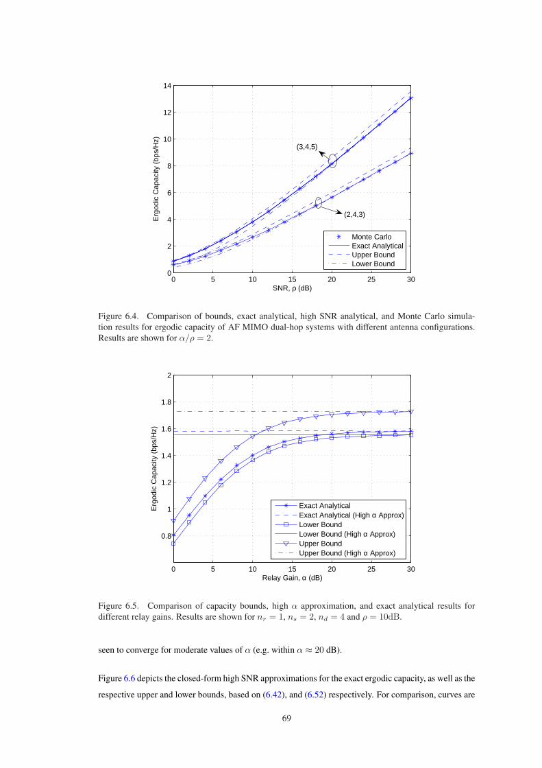
0 5 10 15 20 25 300

2

4

6

8

10

12

14

SNR, ρ (dB)

Erg

odic

Cap

acity

(bp

s/H

z)

Monte CarloExact AnalyticalUpper BoundLower Bound

(2,4,3)

(3,4,5)

Figure 6.4. Comparison of bounds, exact analytical, high SNR analytical, and Monte Carlo simula-tion results for ergodic capacity of AF MIMO dual-hop systems with different antenna configurations.Results are shown for α/ρ = 2.

0 5 10 15 20 25 30

0.8

1

1.2

1.4

1.6

1.8

2

Relay Gain, α (dB)

Erg

odic

Cap

acity

(bp

s/H

z)

Exact AnalyticalExact Analytical (High α Approx)Lower BoundLower Bound (High α Approx)Upper BoundUpper Bound (High α Approx)

Figure 6.5. Comparison of capacity bounds, high α approximation, and exact analytical results fordifferent relay gains. Results are shown for nr = 1, ns = 2, nd = 4 and ρ = 10dB.

seen to converge for moderate values of α (e.g. within α ≈ 20 dB).

Figure 6.6 depicts the closed-form high SNR approximations for the exact ergodic capacity, as well as the

respective upper and lower bounds, based on (6.42), and (6.52) respectively. For comparison, curves are

69

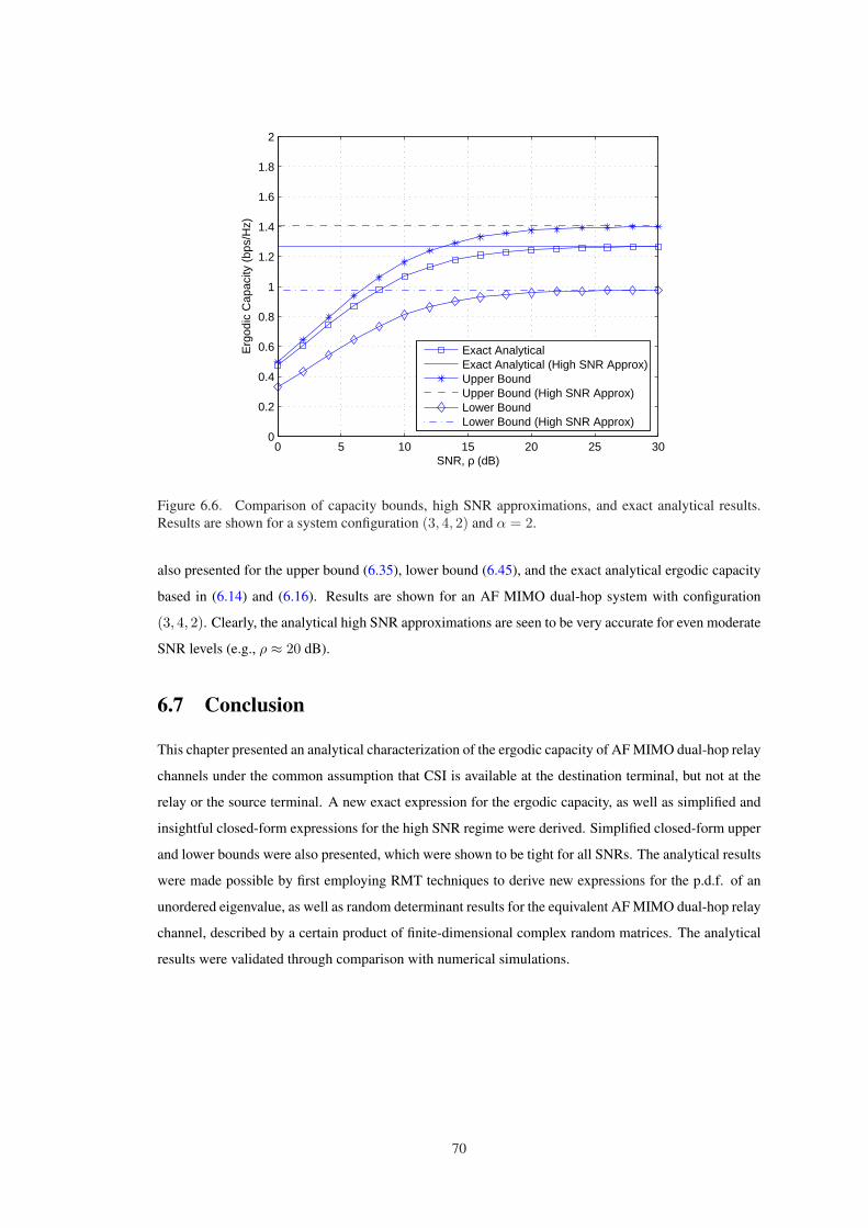
0 5 10 15 20 25 300

0.2

0.4

0.6

0.8

1

1.2

1.4

1.6

1.8

2

SNR, ρ (dB)

Erg

odic

Cap

acity

(bp

s/H

z)

Exact AnalyticalExact Analytical (High SNR Approx)Upper BoundUpper Bound (High SNR Approx)Lower BoundLower Bound (High SNR Approx)

Figure 6.6. Comparison of capacity bounds, high SNR approximations, and exact analytical results.Results are shown for a system configuration (3, 4, 2) and α = 2.

also presented for the upper bound (6.35), lower bound (6.45), and the exact analytical ergodic capacity

based in (6.14) and (6.16). Results are shown for an AF MIMO dual-hop system with configuration

(3, 4, 2). Clearly, the analytical high SNR approximations are seen to be very accurate for even moderate

SNR levels (e.g., ρ ≈ 20 dB).

6.7 Conclusion

This chapter presented an analytical characterization of the ergodic capacity of AF MIMO dual-hop relay

channels under the common assumption that CSI is available at the destination terminal, but not at the

relay or the source terminal. A new exact expression for the ergodic capacity, as well as simplified and

insightful closed-form expressions for the high SNR regime were derived. Simplified closed-form upper

and lower bounds were also presented, which were shown to be tight for all SNRs. The analytical results

were made possible by first employing RMT techniques to derive new expressions for the p.d.f. of an

unordered eigenvalue, as well as random determinant results for the equivalent AF MIMO dual-hop relay

channel, described by a certain product of finite-dimensional complex random matrices. The analytical

results were validated through comparison with numerical simulations.

70

Chapter 7

Performance Analysis of OC in

Rayleigh-Product Channels

7.1 Introduction

Wireless communications systems are generally subjected to co-channel interferences. For multiple an-

tenna systems, OC scheme which maximizes the received SINR by exploiting the CSI in a SIMO antenna

system has been proposed in [100] to combat the effect of co-channel interference. Later in [103], the

concept of OC was extended to a MIMO antenna system in which the transmit and receive antennas are

jointly optimized to maximize the SINR by projecting the transmitted signal onto the strongest eigen-

space of the interference-inverted channel matrix in quadratic form. The performance of OC systems

have been extensively analyzed in the literature, see e.g., [27, 44, 47, 59–61, 64, 81, 106].

While these prior research works are fundamental in nature and profoundly important in understanding

the performance of the MIMO OC systems, most adopted the assumption of a perfectly rich-scattering

environment that renders a full-rank MIMO channel matrix, Hence, these results tend to be overly opti-

mistic, and may fail to address practical environments such as keyholes [8] or the more general double-

scattering channels [25].

Motivated by this, in this chapter, we intend to provide an accurate account of the real performance of OC

systems operating in double-scattering channels. To allow useful results to be derived, we shall assume

that the transmit and receive antennas are uncorrelated and the scattering matrix in the double-scattering

model is identity, giving rise to a Rayleigh-product MIMO channel with co-channel interference. Fur-

thermore, as in [44], we shall adopt the interference-limited assumption so that noise can be neglected

and also the assumption that the co-channel interferers are of equal power and Rayleigh-faded.

In this chapter, we present the exact closed-form expression for the outage probability of the OP systems

in interference-limited Rayleigh product channel based on the new statistical results derived in Chapter 3.

To gain more insight, we apply these findings to develop further analytical results for the keyhole chan-

nel, an important special case of double scattering channel. In particular, the expressions in closed form

for the p.d.f. and c.d.f. (and their asymptotic expansions), the ergodic capacity, the outage probability

and the SER of the optimally-combined keyhole channel with co-channel interference are derived.

7.2 System Model

Consider a MIMO system equipped with Nt antennas at the transmitter and Nr antennas at the receiver,

and assume that there exist NI co-channel interferers with NI ≥ Nr. The received signals in vector

form can be modeled as

y =√

P0Hts0 +NI∑n=1

√Pnhnsn + η (7.1)

where s0 is the transmitted signal of the desired user, and sn (n ≥ 1) denotes the signals transmitted from

the nth interferer with E[|sn|2] = 1 ∀n so that Pn are the transmitted power of the users. Additionally,

η is the complex noise vector with independent elements following CN (0, σ2), t ∈ CNt denotes the

transmit beamforming vector of the desired user with ‖t‖ = 1, hn ∈ CNr is the complex channel vector

of the nth interferer with independent elements following CN (0, 1), and

H =1√Ns

H1H2 (7.2)

in which H1 ∼ CNNr,Ns(0Nr×Ns

, I ⊗ I) and H2 ∼ CNNs,Nt(0Ns×Nt

, I ⊗ I) are random matrices,

is the Rayleigh-product MIMO channel1 between the transmitter and the desired receiver with Ns being

the number of scatterers in the environment [104]. For ease of exposition, we define HI , [h1 · · ·hn].

As a consequence, (7.1) can be re-expressed as

y =√

P0Hts0 + HIP12I sI + η (7.4)

where PI = diag(P1, . . . , PNI ), and sI = [s1 s2 · · · sNI ]T .

In this model, the desired user’s channel is assumed to undergo double-scattering while the interferences

do not. This setting is particularly useful for an uplink space-division multiple-access (SDMA) system

in which the same spectrum is shared by a number of users within a cell. As a result, it can represent

the scenario where the desired user is at the boundary of the cell and the co-channel interferences (other

users) are much closer to the base station receiver. The double-scattering desired user link with single-

scattering interferers is therefore an important benchmark for the performance of MIMO-SDMA systems

using OC in the uplink.

To allow further analysis of the system, henceforth, we assume that the system is interference-limited,

meaning that the noise can be neglected (though the results of this paper will be examined numerically

1In the double-scattering model [25], the channel matrix in (7.2) would have been written as

H =1√Ns

Σ12 H1Φ

12 H2Ξ

12 (7.3)

where Φ denotes the scatterer correlation matrix, and Σ and Ξ denote, respectively, the spatial correlation matrices at the receiverand the transmitter. Hence, the Rayleigh product model is the special case of the double-scattering model when Σ = Φ = Ξ = I.

72

in the presence of noise in Section 7.4). This assumption is particularly reasonable when the interference

to noise ratio (INR) is high. To make the analysis tractable, we also assume that PI , P1 = P2 = · · · =PNI .

The OC for (7.4) with CSI has been well known [103]. In particular, the optimum receiver combin-

ing, which maximizes the output signal-to-interference ratio (SIR) (with noise being ignored) by left-

multiplying y with a vector r†, is achieved by having

r =(PIHIH

†I)−1

Ht, (7.5)

which gives the SIR, ρ, as

ρ = t†H†(PIHIH

†I)−1

Ht

=1

NsPIt†H†

2H†1

(HIH

†I)−1

H1H2t.(7.6)

According to the Rayleigh-Ritz theorem [30], γ is maximized by choosing t = umax, where umax

denotes the eigenvector corresponding to the largest eigenvalue of the matrix

F , 1Ns

H†2H

†1

(HIH

†I)−1

H1H2. (7.7)

The corresponding maximum SIR is given by

ρmax =P0

PIλmax, (7.8)

where λmax is the largest eigenvalue of F. Apparently, the performance of (7.4) depends directly upon

the statistical properties of λmax.

7.3 Performance Analysis of OC Systems in Rayleigh-Product

Channels

In this section, we study the performance of the OC systems in Rayleigh-product channels based on

a set of newly derived closed-form expressions of the c.d.f. and p.d.f. the maximum eigenvalue λmax

presented in Chapter 3.

7.3.1 Outage Analysis of OC Systems in Rayleigh-Product Channels

Outage probability is an important performance metric in communication systems, which is defined as

the probability that the system fails to achieve an acceptable SIR threshold, say, ρth. In this subsection,

we present the closed-form outage expressions of the OC systems in Rayleigh-product channels.

73

Theorem 7.1 For interference-limited Rayleigh-product channels, the outage probability of the OC sys-

tems can be computed as

1) When Nt ≤ Nr or Nt ≥ Nr ≥ Ns,

Pout =

∏mi=1(−1)pNtΓ(NI + Ns − i + 1) det

(∆

(PIρth

P0

))∏m

i=1 Γ(NI −Nr + m− i + 1)Γ(m− i + 1)Γ(n− i + 1), (7.9)

2) When Nt ≥ Ns ≥ Nr or Ns ≥ Nt ≥ Nr,

Pout =

∏mi=1 Γ(NI + n− i + 1) det

(Θ

(PIρth

P0

))

∏mj=1 Γ(NI − j + 1)Γ(n− j + 1)Γ(m− j + 1)

∏Nt

i=1 Γ(Nt − i + 1), (7.10)

where ∆(x) and Θ(x) is an Nr ×Nr matrix whose entries are defined in Theorem 3.5.

Proof: Following the definition of outage probability, the desired results can be obtained by directly

invoking Theorem 3.5. ¤

The above theorem gives a complete characterization of the outage behavior of OC systems in

interference-limited Rayleigh-product channels. Although these expressions can be efficiently evaluated

by standard softwares, such as Mathematica, the expressions themselves are too complicated to gain

physical insights. In the following section, we consider a special case of Rayleigh-product channels,

namely keyhole channels, for which, we give a detailed performance investigation.

7.3.2 Performance Analysis of OC Systems in Keyhole Channels

In this subsection, we examine, in detail, the keyhole channel which is a special case of double-scattering

or Rayleigh-product channels discussed in Section 7.2. We first give the exact closed-form expressions

for the c.d.f. and p.d.f. when Ns = 1, then derive the asymptotic expressions for the c.d.f. and p.d.f.,

which will enable us to reveal some insightful properties. Using these new statistical results, we also

derive the ergodic capacity, the outage probability and the SER of the keyhole channels.

When Ns = 1, the number of scatterers in the channel is one and this channel is usually referred as the

keyhole, or pinhole, channel.

Corollary 7.1 When Ns = 1, the c.d.f. of the non-zero eigenvalue of F is expressed as

Fλmax(x) = 1− Γ(NI + 1)Γ(Nr)Γ(NI −Nr + 1)

Nt−1∑

k=0

xkΓ(NI −Nr + k + 1)Γ(k + 1)

U(NI −Nr + k + 1, k −Nr + 1, x). (7.11)

Corollary 7.2 When Ns = 1, the p.d.f. of the non-zero eigenvalue of F is given by

fλmax(x) =Γ(NI + 1)Γ(NI + Nt −Nr + 1)

Γ(NI −Nr + 1)Γ(Nt)Γ(Nr)xNt−1U(NI + Nt −Nr + 1, Nt −Nr + 1, x). (7.12)

74

The proofs of the above two corollaries are straightforward and thus omitted.

To this end, we derive the asymptotic expansions for the c.d.f. and p.d.f. of the non-zero eigenvalue of

F. The simple expressions obtained enable us to investigate the asymptotic outage probability later.

Theorem 7.2 The asymptotic expansions for the c.d.f. and p.d.f. of the non-zero eigenvalue of F are

given, respectively, by

Fλmax(x)|Ns=1 = axs +O(xs+1), (7.13)

fλmax(x)|Ns=1 = asxs−1 +O(xs), (7.14)

where s = min(Nt, Nr) and

a =

Γ(NI + Nt −Nr + 1)Γ(Nr −Nt)Γ(NI −Nr + 1)Γ(Nt + 1)Γ(Nr)

,Nt ≤ Nr − 1,

− Γ(NI + 1)[lnx + ψ(NI + 1)]Γ(NI −Nr + 1)Γ(Nt + 1)Γ(Nr)

,Nt = Nr,

Γ(NI + 1)Γ(Nt −Nr)Γ(NI −Nr + 1)Γ(Nt)Γ(Nr + 1)

,Nt ≥ Nr + 1,

(7.15)

where ψ(·) is the digamma function which, for integer n, can be expressed as [26]

ψ(n) = −K +n−1∑p=1

1p, (7.16)

where K ≈ 0.57721566 denotes the Euler’s constant.

Proof: The asymptotic expansion of U(a, b, x) can be obtained from [4, (13.5.6)–(13.5.12)]. Utilizing

these results together with Corollary 7.2, we can get the first-order expansion for the p.d.f. of the keyhole

channel. The c.d.f. is obtained by an additional integration. ¤

7.3.2.1 Ergodic Capacity

Now, we present the ergodic capacity (b/s/Hz) of the MIMO OC system in keyhole channels with co-

channel interference. This is obtained by evaluating

C = Eλmax

[log2

(1 +

P0

PIλmax

)]. (7.17)

Applying the result in Corollary 7.2 and after some mathematical manipulations, (7.17) can be expressed

in closed-form as presented in the following theorem.

75

Theorem 7.3 The ergodic capacity of the interference-limited keyhole channel is given by

C =

log2 eG2,44,3

P0

PI

∣∣∣∣∣∣1, 1, 1−Nt, 1−Nr

1, 1 + NI −Nr, 0

Γ(NI −Nr + 1)Γ(Nt)Γ(Nr), (7.18)

where Gm,np,q

(x

∣∣∣a1,...,ap

b1,...,bq

)is the Meijer-G function defined in [26, (9.301)].

Proof: We start by expressing Hypergeometric function U(·, ·, ·) and ln(1 + x) [76, (8.4.6.5)] in terms

of Meijer-G function, i.e.,

U(a, b, x) =1

Γ(a)Γ(a− b + 1)G2,1

1,2

(x

∣∣∣1−a0,1−b

),

ln(1 + ax) = G1,22,2

(ax

∣∣∣1,11,0

).

(7.19)

The desired result can be obtained with the help of the integration formula [26, (7.821.3)]. ¤

Although the explicit equation given above can be used to compute the ergodic capacity efficiently, it

does not offer much insight about the system. Therefore, it is of interest to analyze the special case

which gives simplified expressions. The following two corollaries characterize the ergodic capacity of

the keyhole channel in the high and low SIR regimes.

Corollary 7.3 In the low SIR regime, for NI > Nr, the ergodic capacity in (7.18) can be expressed as

C ≈ K

(P0

PI

), (7.20)

where

K =NtNr

NI −Nr. (7.21)

Proof: At low SIRs, we can approximate the capacity formula (7.17) as C ≈ P0PI

E[λmax]. Then, utilizing

the integral formula in [26, (7.612.2)] yields

C ≈ Γ(NI + 1)Γ(NI + Nt −Nr + 1)Γ(NI −Nr + 1)Γ(Nt)Γ(Nr)

P0

PI

∫ ∞

0

xNtU(NI + Nt −Nr + 1, Nt −Nr + 1, x)dx

= K

(P0

PI

),

(7.22)

where K has been defined in (7.21). For NI = Nr, nevertheless, due to the capacity approximation at

low SIRs, the integral in (7.22) diverges and such an approximation is not available. ¤

Corollary 7.4 In the high SIR regime, the ergodic capacity in (7.18) allows the following expression

C ≈ log2

P0

PI+ (log2 e)× [ψ(Nr) + ψ(Nt)− ψ(NI −Nr + 1)]. (7.23)

76

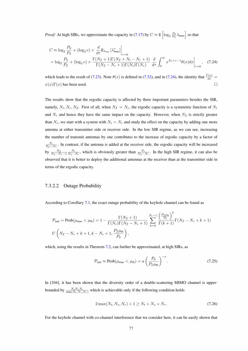
Proof: At high SIRs, we approximate the capacity in (7.17) by C ≈ E[log2

P0PI

λmax

]so that

C ≈ log2

P0

PI+ (log2 e)× d

dτEλmax [λτ

max]∣∣∣∣τ=0

= log2

P0

PI+ (log2 e)× Γ(NI + 1)Γ(NI + Nt −Nr + 1)

Γ(NI −Nr + 1)Γ(Nt)Γ(Nr)d

dτ

∫ ∞

0

xNt+τ−1θ(x)dx

∣∣∣∣τ=0

, (7.24)

which leads to the result of (7.23). Note θ(x) is defined in (7.32), and in (7.24), the identity that Γ(x)dx =

ψ(x)Γ(x) has been used. ¤

The results show that the ergodic capacity is affected by three important parameters besides the SIR,

namely, Nt, Nr, NI . First of all, when NI = Nr, the ergodic capacity is a symmetric function of Nt

and Nr and hence they have the same impact on the capacity. However, when NI is strictly greater

than Nr, we start with a system with Nt = Nr and study the effect on the capacity by adding one more

antenna at either transmitter side or receiver side. In the low SIR regime, as we can see, increasing

the number of transmit antennas by one contributes to the increase of ergodic capacity by a factor ofNr

NI−Nr. In contrast, if the antenna is added at the receiver side, the ergodic capacity will be increased

by NINI−Nr−1

Nr

NI−Nr, which is obviously greater than Nr

NI−Nr. In the high SIR regime, it can also be

observed that it is better to deploy the additional antennas at the receiver than at the transmitter side in

terms of the ergodic capacity.

7.3.2.2 Outage Probability

According to Corollary 7.1, the exact outage probability of the keyhole channel can be found as

Pout = Prob(ρmax < ρth) = 1− Γ(NI + 1)Γ(Nr)Γ(NI −Nr + 1)

Nt−1∑

k=0

(PIρth

P0

)k

Γ(k + 1)Γ(NI −Nr + k + 1)

U

(NI −Nr + k + 1, k −Nr + 1,

PIρth

P0

),

which, using the results in Theorem 7.2, can further be approximated, at high SIRs, as

Pout ≈ Prob(ρmax < ρth) = a

(P0

PIρth

)−s

. (7.25)

In [104], it has been shown that the diversity order of a double-scattering MIMO channel is upper-

bounded by NtNsNr

max(Nt,Ns,Nr) which is achievable only if the following condition holds

2max(Nt, Ns, Nr) + 1 ≥ Nt + Ns + Nr. (7.26)

For the keyhole channel with co-channel interference that we consider here, it can be easily shown that

77

this condition is satisfied and therefore

Diversity Gain =NtNr

max(Nt, 1, Nr)= min(Nt, Nr), (7.27)

which coincides with the asymptotic result in (7.13). Intriguingly, note also that the diversity order does

not depend on the number of co-channel interferers NI which turns out to affect only the coding (or

array) gain of the system. To exemplify this, let us focus on (7.15) for the case Nt ≤ Nr − 1. When the

number of interferers increases from, say, NI to NI = NI + 1, then we have

a(NI)

=Γ(NI + Nt −Nr + 1)Γ(Nr −Nt)Γ(NI −Nr + 1)Γ(Nt + 1)Γ(Nr)

=NI + Nt −Nr + 1

NI −Nr + 1Γ(NI + Nt −Nr + 1)Γ(Nr −Nt)Γ(NI −Nr + 1)Γ(Nt + 1)Γ(Nr)

> a(NI). (7.28)

As a result, a increases with the number of interferers, which in turn decreases the coding gain because

CODING GAIN =(

1a

) 1s

. (7.29)

In addition, (7.15) demonstrates that both the c.d.f. and the p.d.f. of λmax decay to zero more slowly for

Nt = Nr than for Nt 6= Nr, due to the term lnx in the leading factor a.

7.3.2.3 SER

In addition to the outage probability, SER is also a common metric used to characterize the performance

of a communication system. For most modulation formats, the average SER can be evaluated as [75]

SER(

P0

PI

)= Eρmax

[αQ

(√2βρmax

)], (7.30)

where Q(·) is the Gaussian Q-function, and α, β are modulation-specific constants. For example, BPSK

requires α = 1, β = 1; BFSK has α = 1, β = 0.5 with orthogonal signaling or α = 1, β = 0.715 with

minimum correlation while for M -ary PAM, α = 2(M − 1)/M, β = 3/(M2 − 1).

Theorem 7.4 The SER of the interference-limited keyhole channel is given by

SER(

P0

PI

)=

αG3,23,3

βP0

PI

∣∣∣∣∣∣1−Nt, 1−Nr, 1

0, 1/2, 1 + NI −Nr

2√

πΓ(NI −Nr + 1)Γ(Nt)Γ(Nr). (7.31)

Proof: Define

θ(x) ∆= U(NI + Nt −Nr + 1, Nt −Nr + 1, x). (7.32)

78

Making use of (7.8) and Corollary 7.2, the SER of keyhole channel can be evaluated as

SER(

P0

PI

)=

∫ ∞

0

[αQ

(√2β

P0

PIx

)]fλmax(x)dx

=αΓ(NI + 1)Γ(NI + Nt −Nr + 1)

Γ(NI −Nr + 1)Γ(Nt)Γ(Nr)

∫ ∞

0

[Q

(√2β

P0

PIx

)xNt−1θ(x)

]dx.

(7.33)

Utilizing the relation that Q(x) = 12erfc

(x√2

), where erfc(·) denotes the complementary error function

[26], we express erfc(x) in terms of Meijer-G function as [76]

erfc(√

x) =1√π

G2,01,2

(x

∣∣∣10,1/2

). (7.34)

Now, applying (7.19), (7.34), and integrating using [26, (7.821.3)] yields the desired result. ¤

7.4 Numerical Results

In this section, we provide numerical results to confirm the correctness of the analytical results we

have derived. In addition to that, various examples are also given to demonstrate how various system

parameters impact on the performance of a Rayleigh-product MIMO channel using OC. In particular,

we validate our two assumptions, namely, “equal power interference”, and ”interference-limited”, we

show that the assumed model can provide very good performance reference to the real system. All the

simulation results are obtained based on 1,000,000 independent channel realizations.

Figure 7.1 plots the outage probability Pout versus the normalized SIR (i.e., the SIR normalized by the

threshold) P0/(PIρth) for various number of scatterers Ns when Nt = 3, Nr = 5, and NI = 6. Results

in this figure indicate that the number of scatterers has a significant impact on the outage performance,

which agrees with the expectation that the number of scatterers should somehow link with the diversity

order of the channel which affects the outage probability. In addition, as can be seen in Figure 7.1, the

results for both the Monte Carlo simulations and the analytical formulae agree perfectly with each other.

Figure 7.2 provides similar results as in Figure 7.1 but for various number of co-channel interferers NI

for two settings when (Nt, Nr, Ns) = (3, 4, 1), and (Nt, Nr, Ns) = (3, 4, 5). It shows that a larger

number of co-channel interferers degrades the system performance and leads to an increase in the outage

probability. Also, intriguingly, it is observed that NI affects only on the coding gain but not the diversity

order.

Now, numerical results in Figure 7.3 and Figure 7.4 are provided for the outage probability performance

when (Nt, Nr, Ns) = (3, 4, 7) under the case when the interference-limited system and equal-power

interferers assumptions are no longer true. In Figure 7.3, we compare the analytical results to Monte

Carlo results for the system with equal power interference PIσ2 = 3 (dB) plus white Gaussian noise.

While in Figure 7.4, we plot the analytical results against the Monte Carlo results for the system with

unequal power inteference Pi = 2i−1NI

PI and white Gaussian noise. A close observation from the results

79

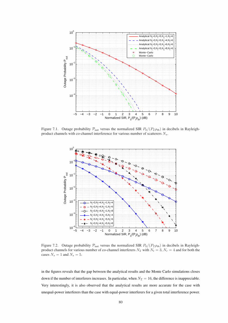
−5 −4 −3 −2 −1 0 1 2 3 4 5 6 7 8 9 10

10−4

10−3

10−2

10−1

100

Normalized SIR, P0/(P

Iρ

th) (dB)

Out

age

Pro

babi

lity

Pou

t

Analytical Nt=3,N

r=5,N

s=1,N

I=6

Analytical Nt=3,N

r=5,N

s=4,N

I=6

Analytical Nt=3,N

r=5,N

s=6,N

I=6

Analytical Nt=3,N

r=5,N

s=8,N

I=6

Monte−CarloMonte−Carlo

Figure 7.1. Outage probability Pout versus the normalized SIR P0/(PIρth) in decibels in Rayleigh-product channels with co-channel interference for various number of scatterers Ns.

−5 −4 −3 −2 −1 0 1 2 3 4 5 6 7 8 9 1010

−6

10−5

10−4

10−3

10−2

10−1

100

Normalized SIR, P0/(P

Iρ

th) (dB)

Out

age

Pro

babi

lity

Pou

t

Nt=3,N

r=4,N

s=1,N

I=4

Nt=3,N

r=4,N

s=1,N

I=6

Nt=3,N

r=4,N

s=1,N

I=8

Nt=3,N

r=4,N

s=5,N

I=4

Nt=3,N

r=4,N

s=5,N

I=6

Nt=3,N

r=4,N

s=5,N

I=8

Figure 7.2. Outage probability Pout versus the normalized SIR P0/(PIρth) in decibels in Rayleigh-product channels for various number of co-channel interferers NI with Nt = 3, Nr = 4 and for both thecases Ns = 1 and Ns = 5.

in the figures reveals that the gap between the analytical results and the Monte Carlo simulations closes

down if the number of interferers increases. In particular, when NI = 16, the difference is inappreciable.

Very interestingly, it is also observed that the analytical results are more accurate for the case with

unequal-power interferers than the case with equal-power interferers for a given total interference power.

80

−10 −9 −8 −7 −6 −5 −4 −3 −2 −1 0 1 2 3 4 510

−4

10−3

10−2

10−1

100

Normalized SIR, P0/(P

Iρ

th) (dB)

Out

age

Pro

babi

lity

Pou

t

Monte−CarloAnalytical, N

t=3, N

r = 4, N

s = 7, N

I=8

Monte−CarloAnalytical, N

t=3, N

r = 4, N

s = 7, N

I=12

Monte−CarloAnalytical, N

t=3, N

r = 4, N

s = 7, N

I=16

Figure 7.3. Outage probabilityPout versus the normalized SIR P0/(PIρth) in decibels with equal-powerco-channel interferers and white noise.

−10 −9 −8 −7 −6 −5 −4 −3 −2 −1 0 1 2 3 4 510

−4

10−3

10−2

10−1

100

Normalized SIR P0/(P

Iρ

th) (dB)

Out

age

Pro

babi

lity

Pou

t

Monte−CarloAnalytical, N

t=3,N

r=4,N

s=7,N

I=8

Monte−CarloAnalytical, N

t=3,N

r=4,N

s=7,N

I=12

Monte−CarloAnalytical, N

t=3,N

r=4,N

s=7,N

I=16

Figure 7.4. Outage probability Pout versus the normalized SIR P0/(PIρth) in decibels with unequal-power co-channel interferers Pi = 2i−1

NIPI , for i = 1, . . . , NI and white noise.

Results in Figs. 7.5–7.7 are provided for keyhole MIMO channels (i.e., Ns = 1). Figure 7.5 illustrates

the outage probability results for various number of transmit antennas Nt when Nr = 5 and NI = 6.

The results for the exact analytical expression (7.11), the asymptotic expression (7.13) and the Monte-

Carlo simulations are shown and compared. As we can see, the Monte Carlo and the exact analytical

81

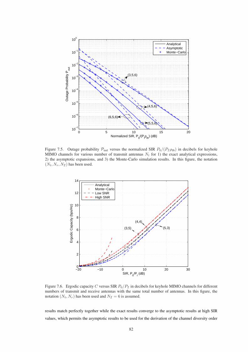
0 5 10 15 2010

−7

10−6

10−5

10−4

10−3

10−2

10−1

100

Normalized SIR, P0/(P

Iρ

th) (dB)

Out

age

Pro

babi

lity

Pou

t

AnalyticalAsymptoticMonte−Carlo

(6,5,6)

(5,5,6)

(4,5,6)

(3,5,6)

Figure 7.5. Outage probability Pout versus the normalized SIR P0/(PIρth) in decibels for keyholeMIMO channels for various number of transmit antennas Nt for 1) the exact analytical expressions,2) the asymptotic expansions, and 3) the Monte-Carlo simulation results. In this figure, the notation(Nt, Nr, NI) has been used.

−20 −10 0 10 20 300

2

4

6

8

10

12

14

SIR, P0/P

I (dB)

Erg

odic

Cap

acity

(bp

s/H

z)

AnalyticalMonte−CarloLow SNR High SNR

(3,5)

(4,4)

(5,3)

Figure 7.6. Ergodic capacity C versus SIR P0/PI in decibels for keyhole MIMO channels for differentnumbers of transmit and receive antennas with the same total number of antennas. In this figure, thenotation (Nt, Nr) has been used and NI = 6 is assumed.

results match perfectly together while the exact results converge to the asymptotic results at high SIR

values, which permits the asymptotic results to be used for the derivation of the channel diversity order

82

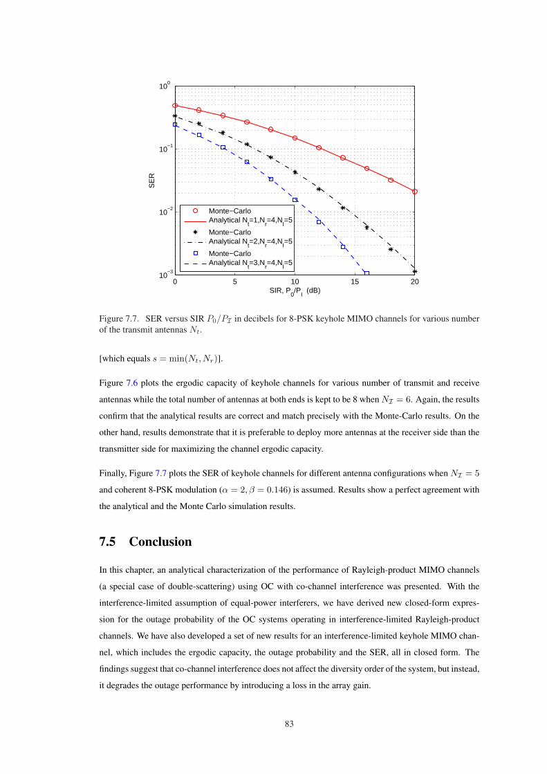
0 5 10 15 2010

−3

10−2

10−1

100

SIR, P0/P

I (dB)

SE

R

Monte−CarloAnalytical N

t=1,N

r=4,N

I=5

Monte−CarloAnalytical N

t=2,N

r=4,N

I=5

Monte−CarloAnalytical N

t=3,N

r=4,N

I=5

Figure 7.7. SER versus SIR P0/PI in decibels for 8-PSK keyhole MIMO channels for various numberof the transmit antennas Nt.

[which equals s = min(Nt, Nr)].

Figure 7.6 plots the ergodic capacity of keyhole channels for various number of transmit and receive

antennas while the total number of antennas at both ends is kept to be 8 when NI = 6. Again, the results

confirm that the analytical results are correct and match precisely with the Monte-Carlo results. On the

other hand, results demonstrate that it is preferable to deploy more antennas at the receiver side than the

transmitter side for maximizing the channel ergodic capacity.

Finally, Figure 7.7 plots the SER of keyhole channels for different antenna configurations when NI = 5

and coherent 8-PSK modulation (α = 2, β = 0.146) is assumed. Results show a perfect agreement with

the analytical and the Monte Carlo simulation results.

7.5 Conclusion

In this chapter, an analytical characterization of the performance of Rayleigh-product MIMO channels

(a special case of double-scattering) using OC with co-channel interference was presented. With the

interference-limited assumption of equal-power interferers, we have derived new closed-form expres-

sion for the outage probability of the OC systems operating in interference-limited Rayleigh-product

channels. We have also developed a set of new results for an interference-limited keyhole MIMO chan-

nel, which includes the ergodic capacity, the outage probability and the SER, all in closed form. The

findings suggest that co-channel interference does not affect the diversity order of the system, but instead,

it degrades the outage performance by introducing a loss in the array gain.

83

Chapter 8

Low SNR Capacity Analysis of General

MIMO Channels with Single Interferer

8.1 Introduction

A wide variety of digital communication systems (e.g., wireless sensor networks) operate in the low-

power region where both spectral efficiency and the energy-per-bit are relatively low. In [95], Verdu

proposed that the spectral efficiency in the low SNR (or wideband) regime can be analyzed through

two parameters; namely, the minimum Eb/N0 (with Eb denoting the average energy per information bit

and N0 being the noise spectral density) required for reliable communications, and the wideband slope

(denoted by S0). These low SNR metrics provide a useful reference in understanding the achievable rate

at low SNRs, and have subsequently been elaborated in [39, 41, 56, 77, 93, 109], where the impacts of

Rician K factor, spatial correlation, transmit and receiver CSI were investigated.

On the other hand, due to spectrum scarcity, communication systems are anticipated to be corrupted by

interference. Therefore, it is of practical interest to investigate the low SNR capacity of MIMO systems

in the presence of co-channel interference. Prior works on this topic were very limited in that explicit

expressions for these two low SNR metrics were only derived for the interference-limited Rayleigh

fading channels, the corresponding results for MIMO Rician fading channels appear to be limited [93].

Motivated by this, in this chapter, we first investigate the MIMO Rician fading channels with arbitrary

mean matrix and K factor, in which we derive exact expressions for Eb/N0min and S0 in the presence

of both interference and noise. Based on these, we further study the special cases, namely, the Rician

MISO channels, the rank-one deterministic channels and the MIMO Rayleigh channels, in which simple

expressions can be obtained to illustrate the impacts of the number of transmit and receive antennas, the

Rician K factor, the channel mean matrix, and the INR on the capacity. Also, asymptotic results in the

large-system limit and high INR are developed. In addition, we provide the low SNR capacity analysis

for Rayleigh-product MIMO fading channels [25] with interference.

8.2 System Model

Consider a communication link with Nt transmit and Nr receive antennas, corrupted by interference and

AWGN. The received signals, y ∈ CNr×1, can be expressed as1

y = Hx + hs + n, (8.1)

where x ∈ CNt×1 is the transmitted symbol vector satisfying E‖x‖2 = P , s is the interference

symbol such that E|s|2 = PI , n ∈ CNr×1 is the noise vector with i.i.d. entries following CN (0, N0),

and H ∈ CNr×Nt denotes the MIMO channel between the transmitter and receiver while h ∈ CNr×1

denotes the channel vector between the interferer and the desired receiver.

In this paper, we investigate the low SNR capacity properties of two important MIMO channel models,

namely: 1) Rician fading and 2) Rayleigh-product fading. They are described as follows:

• Rician MIMO channels—In this case, the channel matrix has the structure [20]

H =

√K

K + 1H0 +

√1

K + 1Hw, (8.2)

where K denotes the Rician K-factor, and Hw ∈ CNr×Nt is the channel matrix containing

i.i.d. zero-mean unit-variance complex Gaussian entries. On the other hand, H0 ∈ CNr×Nt de-

notes the channel mean matrix, which is normalized to satisfy

trH0H

†0

= NrNt. (8.3)

• Rayleigh-product MIMO channels—The channel matrix H can be expressed as [25]

H =1√Ns

H1H2, (8.4)

where H1 ∈ CNr×Ns and H2 ∈ CNs×Nt are statistically independent matrices containing i.i.d.

zero-mean unit-variance complex Gaussian entries, with Ns denoting the number of effective scat-

terers. By varying Ns, this model can describe various rank-deficient effects of a MIMO channel,

e.g., it degenerates to Rayleigh fading if Ns →∞, and a keyhole channel if Ns = 1.

We assume that CSI is not known at the transmitter side but perfectly known at the receiver. Thus, an

equal-power allocation policy is employed and the ergodic capacity is then expressed as [56]

C = E

log2 det

(I +

P

N0NtH†

(PI

N0hh† + I

)−1

H

). (8.5)

1For mathematic tractability, we assume a single co-channel interferer.

85

As pointed out in [56], with co-channel interference, it is more suitable to define the SNR as

ρ ,(

P

N0

)E

tr

H†(ρIhh† + I)−1H

NtNr, (8.6)

where ρI , PI

N0is regarded as the INR. This definition is different from the conventional one which

defines the SNR as the average signal power divided by the noise power. The reason is that in the

presence of interference, the noise is generally colored and SNR should be defined by averaging the

SNRs along each of the principal directions of the noise space.

Based on the above definitions, the ergodic capacity expression in (8.5) can be rewriten as

C(ρ) = E

log2 det

(I +

ρH† (ρIhh† + I

)−1H

1Nr

E tr H†(ρIhh† + I)−1H

). (8.7)

At low SNRs, it has proved useful to investigate the capacity in terms of the normalized transmit energy

per information bit, Eb/N0, rather than the per-symbol SNR, ρ. This capacity can be well approximated

for low Eb/N0 levels by the following expression [95]

C

(Eb

N0

)≈ S0 log2

(Eb

N0Eb

N0 min

), (8.8)

in which Eb

N0 mindenotes the minimum energy per information bit required to convey any positive rate

reliably and S0 is the wideband slope [56, 95]. These are the two key parameters that dictate the capacity

behavior in the low SNR regime, and can be obtained from C(ρ) via [56]2

Eb

N0 min

=NtNr

E tr H†(ρIhh† + I)−1H1

C(0), (8.9)

S0 = −2

[C(0)

]2

..

C(0)ln 2, (8.10)

where C(·) and..

C(·) represent, respectively, the first- and second-order derivatives taken with respect to

ρ. Note that C(

Eb

N0

)implicity captures the second-order behavior of C(ρ) as ρ → 0.

2To facilitate the comparison to the interference free results, we adopt a slightly different definition of EbN0 min

from that in [56].Specifically, in [56], Eb is normalized by the interference energy plus the noise energy while here Eb is normalized by the noiseenergy only. Therefore, the final result of Eb

N0 mindiffers by a factor of ρI + 1.

86

8.3 Preliminaries

Here, we present some statistical results that will be used frequently in the following sections. For

notational convenience, we define

D1(m, t) , t−mΨ(m,m, t−1

), (8.11)

D2(m, t) , t−mΨ(m,m− 1, t−1

), (8.12)

where Ψ(·, ·, ·) is the confluent hypergeometric function defined in [26].

Lemma 8.1 For any m× 1 vector h ∼ CN (0, I), and positive number t, let Λ ∆= (thh† + I)−1. Then,

we have

E tr Λ = m− 1 + D1(m, t), (8.13)

Etr

Λ2

= m− 1 + D2(m, t), (8.14)

Etr2 Λ = (m− 1)2 + 2(m− 1)D1(m, t) + D2(m, t). (8.15)

Proof: The result can be obtained by noting the unitary invariant of vector h, and using the integration

formula [26, (3.385.5)]. ¤

Lemma 8.2 For any m × n matrix H ∼ CN (0, I ⊗ I), m × 1 vector h ∼ CN (0, I), and positive

constant t, we have

EtrH†ΛH = n(m− 1) + nD1(m, t), (8.16)

Etr(H†ΛH)2 = n(m− 1)(n + m− 1) + (n2 + n)D2(m, t) + 2n(m− 1)D1(m, t), (8.17)

Etr2H†ΛH = n(m− 1)(mn− n + 1) + (n2 + n)D2(m, t) + 2(m− 1)n2D1(m, t), (8.18)

where Λ has been defined in Lemma 8.1.

Proof: See Appendix E.1. ¤

Lemma 8.3 When m → ∞ or t → ∞, we have D1(m, t) = D2(m, t) = 0. On the other hand, if

t → 0, D1(m, t) = D2(m, t) = 1.

Proof: See Appendix E.2. ¤

87

8.4 Low SNR Capacity Analysis of Rician MIMO Channels with

Single Interferer

In this section, we derive analytical expressions for Eb/N0min and the wideband slope, S0, for Rician

MIMO fading channels. The main result is given in the following theorem.

Theorem 8.1 For MIMO Rician fading channels with a single interferer, we have

Eb

N0 min

=ln 2

Nr − 1 + A0, (8.19)

S0 =2Nt(K + 1)2

2K + B0, (8.20)

where A0 and B0 are, respectively, given by

A0 = D1(Nr, ρI), (8.21)

and

B0 =1

(Nr − 1 + D1(Nr, ρI))2

2K2

(tr

(H0H

†0)

2−N2

t Nr

)

Nt(Nr + 1)+ 2(Nr − 1)

D1(Nr, ρI)

+

1 + (1 + 2K)Nt +

K2(tr

(H0H

†0)

2

+ N2t N2

r

)

NtNr(Nr + 1)

D2(Nr, ρI)

+(Nr − 1)

Nr − 1 + (1 + 2K)Nt +

K2(tr

(H0H

†0)

2

(N2r −Nr − 1) + N2

t N2r

)

NtNr(N2r − 1)

. (8.22)

Proof: See Appendix E.3. ¤

Theorem 8.1 is general and valid for mean matrix of arbitrary rank, H0, and any possible Nt, Nr, K

and ρI . From (8.19), we observe that the Rician factor K and the structure of channel mean H0 (as long

as trH0H

†0

= NtNr) do not affect Eb/N0min, while the values of Nr and ρI have a direct impact.

Also in (8.20), we see that all the parameters will affect the wideband slope S0.

Based on (8.19), we can further investigate the impact of Nr and ρI on Eb/N0min as follows.

Corollary 8.1 The Eb/N0min is a decreasing function of Nr (i.e., when Nr increases, Eb/N0min de-

creases) and is an increasing function of ρI (i.e., when ρI increases, Eb/N0min increases). Moreover,

the increase in Eb/N0min due to interference is upper bounded by ln 2Nr(Nr−1) for Nr ≥ 2.

Proof: See Appendix E.4. ¤

88

Corollary 8.2 When ρI → 0, Theorem 8.1 reduces to

Eb

N0 min

=ln 2Nr

, (8.23)

S0 =2(K + 1)2

K2tr(H0H†0)

2N2

t N2r

+ (1 + 2K)Nt+Nr

NtNr

. (8.24)

In particular, if the channel mean matrix, H0, is of rank-1, then S0 can be reduced to

S0 =2(K + 1)2

K2 + (1 + 2K)Nt+Nr

NtNr

. (8.25)

Proof: The results can be obtained with the help of Lemma 3, together with the fact that

tr

(H0H†0)

2

= N2t N2

r when H0 is of rank-1. ¤

Corollary 8.2 corresponds to the results for Rician MIMO fading channels in an interference-free envi-

ronment, which generalizes the results in [56] where a rank-1 channel mean was considered.

To gain further insight, in the following, we look at three special cases: 1) Rician MISO fading channels,

i.e., Nr = 1, 2) Rician MIMO channels of rank-1 mean in the large K regime, i.e., K → ∞ and

H0 = αβ† (with complex column vectors α,β), and 3) Rayleigh MIMO channels, i.e., K = 0.

8.4.1 Rician MISO Channels

Corollary 8.3 For Rician MISO channels, i.e., Nr = 1, we have

Eb

N0 min

=ln 2

D1(1, ρI), (8.26)

S0 =2Nt(K + 1)2D1(1, ρI)2

2K + [1 + Nt(1 + K)2]D2(1, ρI). (8.27)

Proof: The result can be obtained by substituting Nr = 1 in Theorem 8.1. ¤

Corollary 8.4 When Nr = 1, S0 is an increasing function of Nt. When 0 ≤ K < 1−D2(1, ρI), S0 is

a decreasing function of K, while for K ≥ 1−D2(1, ρI), S0 is an increasing function of K.

Proof: See Appendix E.5. ¤

In contrast to the interference-free case, where the increase of Rician factor K always improves the

wideband slope S0 when Nr = 1, Corollary 8.4 reveals that the impact of K on S0 depends on the

interference level. Moreover, when ρI → ∞, S0 = 0 which aligns with the observations in [56]

for interference-limited Rayleigh fading scenarios. However, the general impact of ρI on S0 is more

difficult to characterize, though simulation results indicate that S0 decreases when ρI increases.

89

8.4.2 Rank-1 Mean Rician MIMO Channels for Large K

Corollary 8.5 In the large K regime, for rank-1 mean Rician MIMO channels with a single interferer,

it can be derived that

Eb

N0 min

=ln 2

Nr − 1 + A0, (8.28)

S0 =2(Nr + 1)(Nr − 1 + D1(Nr, ρI))2

Nr[Nr(Nr − 1) + 2(Nr − 1)D1(Nr, ρI) + 2D2(Nr, ρI)], (8.29)

Proof: The desired results can be obtained by taking the limit K →∞ in Theorem 8.1. ¤

Corollary 8.5 indicates that in the large K regime, for rank-1 mean Rician MIMO fading channels,

multiple transmit antennas are irrelevant in terms of Eb/N0min and S0. This is actually an intuitive

result. The reason is that the large K regime corresponds to the non-fading channel scenarios, and thus,

varying the number of transmit antennas for a fixed total transmit power will not increase the receive

signal energy and will not contribute to the capacity. In addition, Nr affects both Eb/N0min and S0 in

contrast to the interference-free case where Nr is only relevant in terms of Eb/N0min [56].

With the help of Lemma 8.3, we can further obtain the results in various asymptotic regimes:

• When ρI → 0, Corollary 8.5 reduces to

Eb

N0 min

=ln 2Nr

, (8.30)

S0 = 2. (8.31)

The above results correspond to the interference-free scenario, and conforms to those in [56].

• When Nr →∞, Corollary 8.5 reduces to

Eb

N0 min

=ln 2

Nr − 1, (8.32)

S0 = 2(

1− 1N2

r

)≈ 2. (8.33)

Compared with the interference-free case, the above results suggest that interference degrade the

capacity performance by increasing Eb/N0min and decreasing S0. The loss in Eb/N0min can be

explained by the fact that one receive antenna is dedicated to suppress the single-antenna interfer-

ence, while the rest, Nr − 1 antennas, contribute to normal communication.

• When ρI →∞ and Nr ≥ 2, Corollary 8.5 reduces to

Eb

N0 min

=ln 2

Nr − 1, (8.34)

S0 = 2(

1− 1N2

r

). (8.35)

90

Intriguingly, these results coincide with the case Nr → ∞. Nevertheless, it is worth mentioning

that the situations in application are very different. One is applicable for large Nr but arbitrary

interference power ρI , while the other is valid for large ρI but arbitrary Nr.

8.4.3 Rayleigh MIMO Channels

Corollary 8.6 For Rayleigh MIMO channels with a single interferer, we have

Eb

N0 min

=ln 2

Nr − 1 + A0, (8.36)

S0 =2Nt

1 + B1, (8.37)

where B1 is defined as

B1 , Nt(Nr − 1) + (Nt + 1)D2(Nr, ρI)−D1(Nr, ρI)2

[Nr − 1 + D1(Nr, ρI)]2. (8.38)

Proof: The results follow immediately by substituting K = 0 into Theorem 8.1. ¤

Corollary 8.6 shows that the number of transmit antennas affects the capacity performance through S0.

More insights can be gained by looking into the asymptotic regimes as follows.

• When ρI → 0, we have

Eb

N0 min

=ln 2Nr

, (8.39)

S0 =2NtNr

Nt + Nr. (8.40)

This scenario corresponds to the case for Rayleigh MIMO channels without interference, and the

results are consistent with those derived in [56].

• When Nr →∞, we have

Eb

N0 min

=ln 2

Nr − 1, (8.41)

S0 =2Nt(Nr − 1)Nt + Nr − 1

. (8.42)

• When ρI →∞ and Nr ≥ 2, we have

Eb

N0 min

=ln 2

Nr − 1, (8.43)

S0 =2Nt(Nr − 1)Nt + Nr − 1

. (8.44)

Similar to the case of rank-1 mean Rician MIMO channels with a large K, it is observed that

the results for Nr → ∞ and ρI → ∞ coincide. In addition, by comparing the above results

91

to the interference-free results, we see that in Rayleigh fading, Eb/N0min and S0 for a MIMO

channel with a single interferer behaves like a channel with one less receive antenna operating in

an interference-free environment, which is different from the large K rank-1 mean Rician MIMO

channel case where S0 does not have this interpretation.

8.5 Low SNR Capacity Analysis of Rayleigh-Product MIMO

Channels with Single Interferer

In this section, we develop the low SNR capacity results for Rayleigh-product MIMO channels.

Theorem 8.2 For Rayleigh-product MIMO channels with a single interferer, we have

Eb

N0 min

=ln 2

Nr − 1 + A0, (8.45)

S0 =2NtNs

Nt + Ns + B2, (8.46)

where A0 has been defined in Theorem 8.1 and B2 is given by

B2 , (Nr − 1)(NtNs + 1) + (Nt + 1)(Ns + 1)D2(Nr, ρI)− (Ns + Nt)D1(Nr, ρI)2

[Nr − 1 + D1(Nr, ρI)]2. (8.47)

Proof: See Appendix E.6. ¤

Theorem 8.2 shows that the Eb/N0min for Rayleigh-product MIMO channels is the same as that for

Rician MIMO fading channels, although the two channels have very different information-carrying ca-

pabilities. As such, the results of Corollary 8.1 also apply for Rayleigh-product channels. Nonetheless,

this is not surprising as has already been reported in [95], and this is the consequence of the noise being

additive Gaussian. This explains that Eb/N0min is not sufficient to indicate the capacity performance

and motivates the need for higher order approximation of the capacity such as the wideband slope, S0,

which is generally different for different channels. In addition, it is observed that Nt and Ns affect the

capacity performance through the wideband slope S0 but not Eb/N0min.

Corollary 8.7 When Ns →∞, the wideband slope for Rayleigh-product fading with a single interferer

becomes the same as that for Rayleigh fading scenarios.

Proof: The corollary can be proved by noting that B2Ns|Ns→∞ = B1. ¤

The above corollary indicates that the Rayleigh-product channels converges to a Rayleigh fading channel

when Ns → ∞. This result is quite intuitive since the large Ns correspondes to a rich scattering

enviornment which is the scenario that fits well with the Rayleigh fading model.

The following asymptotic cases are looked at to gain further understanding.

92

• When ρI → 0, we have

Eb

N0 min

=ln 2Nr

, (8.48)

S0 =2NtNsNr

NtNs + NrNs + NtNr + 1. (8.49)

This scenario corresponds to the interference-free case for Rayleigh-product channels whose re-

sults have been derived in [85]. In addition, when Ns = 1, we further have

S0 =2NtNr

(Nt + 1)(Nr + 1)(8.50)

which provides the wideband slope for keyhole channels.

• When Nr →∞, we have

Eb

N0 min

=ln 2

Nr − 1, (8.51)

S0 =2NtNs(Nr − 1)

NtNs + (Nr − 1)(Ns + Nt) + 1. (8.52)

• When ρI →∞ and Nr ≥ 2, it can be easily shown that Eb/N0min and S0 are, respectively, given

by (8.51) and (8.52). In other words, the results for Nr →∞ and ρ →∞ coincide. Additionally,

similar to Rayleigh MIMO channels, the penalty of having an interferer is illustrated through a

reduction on the number of effective receive antennas by 1.

8.6 Numerical Results

In this section, we perform various simulations to further examine the derived analytical expressions.

All the Monte-Carlo simulation results were obtained by averaging over 105 independent channel real-

izations. For MIMO Rician channels, the mean matrix is generated according to [10]

H0 =L∑

l=1

βlα(θr,l)α(θt,l)T , (8.53)

where βl is the complex amplitude of the lth path, and α(θt,l) and α(θr,l) are the specular array re-

sponses corresponding to the lth dominant path at the transmitter and receiver, respectively. The array

response is defined as [1, ej2πd cos(θ), · · · , ej2πd(N−1) cos(θ)]T where d is the antenna spacing in wave-

lengths. In all simulations, we assume that d = 0.5 at both the transmit and receive sides.

For 3×2 MIMO Rician channels, the mean matrix is constructed by assuming that there are two dominant

paths (i.e., L = 2), with the arriving and departure angles given by θr,1 = θt,1 = π2 + π

8 , θr,2 = θt,2 =π2 − π

8 ,3 respectively. The complex coefficient βl is chosen such that trH0H†0 = NtNr. For rank-1

mean Rician fading MIMO channels, we assume L = 1, β1 = 1 and θr,1 = θt,1 = π2 .

3These angles are randomly chosen for simulation purpose, and our results are applicable to arbitrary angles.

93

−8 −6 −4 −2 0 2 4 6 80

2

4

6

8

10

12

14

16

18

Transmit Eb/N

0 (dB)

Cap

acity

(bp

s/H

z)

Monte Carlo SimulationLow SNR approximation

−6.69 −3.06 0.65

Nr=4

Nr=2

Nr=1

Figure 8.1. Low SNR capacity versus transmit Eb/N0 for various Nr when Nt = 3 and ρI = 0 dB.

Fig. 8.1 investigates the impact of Nr on Eb/N0min. To isolate the effect of Nr, we have set K = 0 to

eliminate the possible impact from channel mean matrix H0. From the results of Fig. 8.1, it can be seen

that the increase of Nr helps to reduce the required Eb/N0min, which confirms the analysis of Corollary

8.1. Moreover, we observe that when Nr increases, so does the wideband slope S0, which indicates the

double benefits of increasing Nr. In addition, when compared with the Monte-Carlo simulation results,

the analytical results show very high accuracy in terms of Eb/N0min, and also the wideband slope S0 if

the SNR of interest is sufficiently low, i.e., below 2 bps/Hz of capacity.

In Fig. 8.2, results for the low SNR capacity approximation are plotted for 3× 2 Rician MIMO channels

with K = 1. Results reveal a good agreement between the analysis and the simulations. We also see

that the increase in the interference power degrades the capacity performance by increasing the required

Eb/N0min, while the impact on S0 is not so pronounced. Furthermore, the increase in Eb/N0min from

a channel without interference to that with a 10 dB of INR is about 0.1, which appears to be very close

to the upper bound we obtained in Corollary 8.1 (ln 2)/(Nr(Nr − 1)) = 0.115.

Results in Fig. 8.3 are provided for the capacity of 3 × 2 MIMO Rician channels for different Rician-

K factors in the low SNR regime according to Theorem 8.1. The curves indicate the accuracy of our

analytical expression and that the range for a good approximation improves if K increases. In particular,

the approximation is very good for the capacity range from 0 to 10, when K = 100. Also, results

demonstrate that the Rician K factor affects the capacity performance through the wideband slope S0

but not the Eb/N0min, and more specifically, the wideband slope S0 increases when K becomes larger.

However, the increase is not very substantial. On the other hand, Fig. 8.4 plots the results for rank-1

mean 3 × 2 MIMO Rician channels in the large K regime both with and without interference. Results

94

−7 −6 −5 −4 −3 −2 −1 00

1

2

3

4

5

6

Transmit Eb/N

0 (dB)

Cap

acity

(bp

s/H

z)

Monte Carlo SimulationLow SNR approximation

−5.2 −4.7

ρI=10dB

ρI=0dB

−6.3

No interference

Figure 8.2. Low SNR capacity versus transmit Eb/N0 for various ρI when Nt = 2 and Nr = 3.

−4 −2 0 2 4 6 80

2

4

6

8

10

12

14

Transmit Eb/N

0 (dB)

Cap

acity

(bp

s/H

z)

Monte Carlo SimulationLow SNR approximation

K=0

K=5

K=100

−4.7

Figure 8.3. Low SNR capacity versus transmit Eb/N0 for various Rician factor K when Nt = 2,Nr = 3 and ρI = 10 dB.

confirm the correctness of the analytical results in Corollary 8.5.

Results in Fig. 8.3 are provided for the capacity of 3 × 2 Rician fading MIMO channels for different

Rician-K factors in the low SNR regime according to Theorem 8.1. The curves indicate the accuracy

of our analytical expression and that the range for a good approximation improves if K increases. In

particular, the approximation is very good for the capacity range from 0 to 10, when K = 100. Also,

95

−8 −7 −6 −5 −4 −3 −2 −1 0 10

0.5

1

1.5

2

2.5

3

3.5

4

4.5

5

Transmit Eb/N

0 (dB)

Cap

acity

(bp

s/H

z)

Monte Carlo SimulationLow SNR approximation

−6.3 −5.2−4.7

No interference

ρI=0dB

ρI=10dB

Figure 8.4. Low SNR capacity versus transmit Eb/N0 for rank-1 mean Rician fading MIMO channelswhen Nt = 2, Nr = 3 and K = 100.

results demonstrate that the Rician K factor affects the capacity performance through the wideband slope

S0 but not the Eb/N0min, and more specifically, the wideband slope S0 increases when K becomes

larger. However, the increase is not very substantial. On the other hand, Fig. 8.4 plots the results for

rank-1 mean 3 × 2 Rician MIMO channels in the large K regime both with and without interference.

Results confirm the correctness of the analytical results in Corollary 8.5.

−15 −10 −5 0 50

5

10

15

20

25

30

35

Transmit Eb/N

0 (dB)

Cap

acity

(bp

s/H

z)

Monte Carlo, Nr=21, ρ

I=10dB

Low SNR approximation

Monte Carlo, Nr=20, no interference

Low SNR approximation, no interference

−14.6

Figure 8.5. Low SNR capacity versus transmit Eb/N0 when Nt = 3 and different Nr and ρI .

96

In Fig. 8.5, we provide the results for Rayleigh MIMO fading channels. Two system configurations

are investigated: one for 3 × 21 channels with a single interferer of ρI = 10 dB, and the other for

3× 20 channels without interference. As we can see, the results of the two systems almost overlap with

inappreciable difference in the low SNR regime, which aligns with our analysis.

−6 −4 −2 0 2 4 60

1

2

3

4

5

6

7

8

9

Transmit Eb/N

0 (dB)

Cap

acity

(bp

s/H

z)

Monte Carlo SimulationLow SNR approximation

−4.6 −1.92

No interference

ρI=10dB

Figure 8.6. Low SNR capacity versus transmit Eb/N0 for Rayleigh-product channel when Nt = 3,Ns = 6 and Nr = 2.

−4 −2 0 2 4 60

1

2

3

4

5

6

7

8

9

Transmit Eb/N

0 (dB)

Cap

acity

(bp

s/H

z)

Monte Carlo, Nr=3, ρ

I=20dB

Low SNR approximationMonte Carlo, N

r=2, no interference

Low SNR approximation, no interference

−4.6

Figure 8.7. Low SNR capacity versus transmit Eb/N0 for Rayleigh-product channel when Nt = 2,Ns = 6 and different Nr and ρI .

97

Results in Figs. 8.6 and 8.7 are provided for Rayleigh-product MIMO channels. Results demonstrate

a good agreement between the analysis and simulations. Additionally, it is observed that the level of

interference increases the required Eb/N0min and reduces the wideband slope S0. On the other hand,

Fig. 8.7 plots the results for two systems both with Nt = 2 and Ns = 6: one with a single strong

interferer of ρI = 20 dB and Nr = 3, and the other with Nt = 2 in an interference-free environment.

Results for both systems overlap in the low SNR regime, which confirms our analysis.

8.7 Conclusion

This chapter has studied the capacity of Rician fading and Rayleigh-product MIMO channels with a

single interferer in the low SNR regime. Exact expressions for the minimum energy per information

bit, Eb/N0min, and the wideband slope, S0, were derived for both channels. Also, we showed that

interference degrades the capacity performance by increasing Eb/N0min and reducing S0. Moreover,

the impact of other system parameters, such as the number of transmit and receive antennas, Rician

factor K, the channel mean matrix H0, were investigated.

98

Chapter 9

Conclusions and Future Works

The theme of this thesis is on the capacity and performance analysis of MIMO antenna systems operating

over general and practical propagation channels. There are primary two key aspects in the thesis: the

first is to give a thorough investigation on the fundamental capacity limits of several important MIMO

channels, while the second is to analyze in details for some practical transmission methods over matrix

product channels. In the following, we summarize the main contributions and insights of this thesis, and

discuss some possible lines for future works.

9.1 Summary of Contributions and Insights

In Chapter 3, a host of new finite RMT results were derived, which provided the essential mathematical

tools for the performance analysis conducted in later chapters.

Chapter 4 presented a unified framework of developing capacity bounds for general MIMO Nakagami-

m fading channels based on majorization theory. By exploiting the majorization relationships between

the eigenvalues and diagonal elements of the random matrix of interest, we derived several capacity

upper bounds and lower bounds for both C-MIMO and D-MIMO systems. Based on these analytical

expressions, a number of insights were obtained:

• The ergodic capacity is a monotonic increasing function of the fading parameter m, i.e. if m

becomes greater, the ergodic capacity increases. This finding is quite intuitive since a greater m

corresponds to less severe fading, and the ergodic capacity is anticipated to increase with m.

• In the large system regime, the ergodic capacity of the system scales linearly with the minimum of

the antenna numbers, and is independent of the fading parameter m. This again is an intuitive find-

ing. Since whatever the value of m, the effect of channel fading could be completely eliminated

with the increasing antenna number.

• Both the path loss and shadowing effects affect the ergodic capacity of the system. The path loss

effect decreases the ergodic capacity as a function of the distance, while the shadowing effect

impacts the ergodic capacity through its mean fading parameter.

Chapter 5 considered the mutual information and outage performance of MIMO multi-keyhole channels.

The results for mutual information were derived by directly invoking the new marginal p.d.f. expression

of a product of random matrices (Thoerem 3.2), as well as certain random determinant (Theorem 3.8)

and log-determinant results (Theorem 3.10) from Chapter 3, while the exact and approximate analytical

outage expressions for MIMO MRC systems were obtained based on those maximum eigenvalue distri-

butions, i.e., Theorem 3.3, and Theorem 3.4. From these analytical results, we obtain the following key

insights:

• The mutual information of MIMO multi-keyhole channels is generally inferior to that of MIMO

Rayleigh channels, and the number of keyholes will significantly affect the mutual information.

For instance, when the keyhole number increases, the mutual information improves, and it gradu-

ally approaches the MIMO Rayleigh mutual information bound when the keyhole number is large

enough.

• For MIMO MRC systems, the outage probability of multi-keyhole MIMO channels can be superior

than that of MIMO Rayleigh channels at high outage regime (or equivalently, at sufficiently low

SNR regime). However, for outage level of practical interest, (e.g., ¡ 0.1), achieving a given outage

level requires lower SNR for MIMO Rayleigh channels compared with multi-keyhole channels.

• The keyhole power distribution does not affect the diversity order of the system, while the number

of keyhole does.

• The impact of keyhole power distribution on the outage performance is characterized through

Schur-concavity, and the findings suggest that the more equally distributed keyhole power, the

better is the outage performance.

• By interpreting the keyhole power matrix as the correlation matrix, the results also apply to one-

sided correlated Rayleigh-product channels. And for MIMO MRC system, this indicates that the

higher the correlation of the channel, the worse the outage performance.

Chapter 6 investigated the capacity of MIMO dual-hop systems employing AF relay node. In contrast

to prior results which primary focus on the asymptotic large antenna regime, we aimed at the finite

antenna system. Therefore, the results are applicable for arbitrary number of transmit, relay and receive

antennas. Exact capacity expression was derived by directly invoking Theorem 3.1 along with some

basic mathematical manipulations, and tight capacity upper bound and lower bound were obtained based

on Theorem 3.7 and Theorem 3.9, respectively. Moreover, several special cases were studied in great

detail. From these analytical results, we see that the ergodic capacity of AF MIMO dual-hop systems is

intimately related to that of single hop MIMO systems.

100

• The multiplexing gain of the system is one-half of the minimum of the numbers of transmit, relay

and destination antennas, where the one-half comes from the fact that two time slots are consumed

for the entire communication.

• When the number of relay antennas grows large, the ergodic capacity of AF MIMO dual-hop sys-

tems becomes one-half of that single hop MIMO systems with same transmit and receive antenna

numbers but a properly adjusted SNR. This equivalent SNR is always smaller than the first hop

SNR, which indicates that no matter how many relay antennas are employed and how much power

is used, the capacity is always smaller than one-half of that single hop MIMO systems with the

same transmit and receive antenna numbers with SNR being the first hop SNR.

• When the number of destination antennas grows large, the ergodic capacity of AF MIMO dual-hop

systems becomes one-half of that of the first hop MIMO systems.

• When the relay power grows large, the ergodic capacity of AF MIMO dual-hop systems becomes

one-half of that of a single hop MIMO systems with the same number of transmit antenna, but with

the receive antenna number being the minimum of the relay and destination antenna numbers.

Chapter 7 examined the impact of co-channel interference in Rayleigh-product channels. The exact

outage probability expressions for optimum combining systems were derived based on Theorem 3.5,

and a detailed performance investigation on the special keyhole channels was carried out. From these

analytical results, we have the following findings:

• The interference does not affect diversity order of the system, but it reduces the outage perfor-

mance by contributing in the loss of array gain.

• The number of scatterers will significantly affect the outage performance, and the outage perfor-

mance improves when the number of scatterers increases.

• For the special keyhole channels, the diversity order equals to the minimum of the transmit and

receive antenna numbers.

Chapter 8 studied the ergodic capacity of general MIMO channels with a single interferer in the low SNR

regime. For both Rician channels and Rayleigh-product channels, exact analytical expressions for the

minimum energy per information bit, Eb/N0min, and wideband slope, S0, were derived. Several special

cases were investigated in detail and the impact of transmit, receive antenna number, Rician K factor,

channel mean matrix and INR on the ergodic capacity were analyzed. We gained the following insights:

• The minimum energy per information bit is the same for Rician channels and Rayleigh-product

channels, while their wideband slopes differ significantly.

• Increasing the number of receive antennas helps to reduce the minimum energy per information bit

required for reliable communication, while increasing the interference power requires more power

to ensure reliable communication, and this extra power can be upper bounded.

101

• The structure of the channel mean matrix does not affect the ergodic capacity.

• For MISO Rician channels, the wideband slope is an increasing function of the transmit antenna

number for small K, but is a decreasing function for large K.

• For large K and rank-1 mean Rician MIMO channels, the transmit antenna number does not affect

the ergodic capacity.

• For Rayleigh-product channels, the number of scatters affects the ergodic capacity through the

wideband slope but not the minimum energy per information bit.

• For both scenarios where either the number of receive antenna is large, or the interference power

is large, the resulting capacity performance with one co-channel interference is equivalent to a

system with the same number of transmit antennas but one less receive antenna in an interference

free environment.

9.2 Future Works

In this section, we discuss several possible extensions of the problems investigated in this thesis.

A substantial portion of the thesis is devoted to the analysis of the newly emerged MIMO channels with

product matrix structure. While the contributions made in the thesis have enhanced our knowledge of the

fundamental limitations of the matrix product channels, nevertheless, much more theoretical works are

needed to gain a thorough and deep understanding of the nature of the MIMO matrix product channels.

We believe that matrix product channels will remain a fruitful area, and more important discoveries are

expected to be made. In the following, we discuss some interesting directions.

The first extension is to consider more general settings. In particular, the MIMO multi-keyhole channel

H = H1AH†2 studied in Chapter 5 is a special case of the more general model, referred to as the MIMO

double scattering channel where the channel matrix is given by H = Φ1/2r H1Φ

1/2s H2Φ

1/2t . It is of

great interest to investigate the joint effect of transmit and receive correlation and rank-deficient phe-

nomenon on the fundamental capacity of the system, as well as on the performance of various practical

transmission schemes, i.e., OSTBC and transmit beamforming receiver combining systems.

Secondly, it is interesting to investigate the performance of practically appealing linear receiver system

(i.e., ZF or MMSE receiver), as well as certain low complexity non-linear receiver system(i.e., ZF-DF

or MMSE-DF receiver). While the performance of these simple receivers in a single MIMO Rayleigh

fading channels has been extensively studied and well understood, there has been no available results in

the literature for MIMO product channels. Therefore, it is important to look into this particular system,

analytically characterize its performance, and compare it with the single MIMO Rayleigh channel case

to gain more insights.

102

In addition, the case where partial CSI (i.e., channel mean, or channel correlation matrix) is available

at the transmitter is also an important research topic. The partial CSI case has been well studied for

the single full rank MIMO channels, where optimum precoding matrix and optimal power allocation

schemes based on various performance metrics such as maximizing ergodic capacity, minimizing the

outage probability, or minimizing the mean square error, have been derived for various scenarios. Making

extension to the matrix product channels is therefore of great interest and importance, and it is expected

that the rank deficiency phenomenon will play a key role in designing the system.

While the partial CSI is a more realistic assumption in most of the cases, limited feedback schemes are

more attractive and practical, and it has received enormous attentions from the research community. In

such systems, instead of feedback the exact channel matrix, only limited number of bits is feeded back

to the transmitter, which greatly eases the demand and requirement on the feedback link. One particular

popular limited feedback schemes is the antenna selection schemes, and its performance has been studied

for two extreme cases, i.e., single full rank MIMO channels, degenerated single keyhole channels. To

bridge the gap, it is therefore important to investigate the case with multiple keyholes. Some interesting

questions arise naturally, i.e., how to select the transmit and receive antennas, whether it achieves the

maximum diversity offered by the multi-keyhole channels.

Another interesting area to look into is the multi-hop communication systems, which has attracted enor-

mous attentions from the research community due to its power saving and coverage extension advan-

tages. As the MIMO technology becomes mature, it is expected that MIMO will be incorporated into

the multi-hop system to form a MIMO multi-hop system. Therefore, analytical characterization of the

performance of MIMO multi-hop system is a very important topic. For MIMO multi-hop channels, in

essence, the effective channel of interest consists a product of multiple independent random matrices

which is a generalization of the double-scattering channel model studied in this thesis. So far, only very

limited asymptotic results are available in literature. It has been demonstrated that the asymptotic results

fail to accurately capture the finite cases, which provides great motivation to investigate the performance

of the system in the finite regime. The key challenge is to obtain the statistical properties of the resultant

random product matrices, and it remains to be seen whether the conditional approach developed in the

thesis can be applied in the general case.

In addition to the aforementioned point-to-point MIMO systems, another exciting area is the multi-user

scenarios. Some preliminary results have been developed in Chapter 7 and Chapter 8, where the impact

of co-channel interference is investigated. However, a number of questions remains to be addressed. To

name a few, what is the optimal transmit precoding strategy for each individual user, what is the optimal

power allocation scheme, what the the sum capacity of the system, and what is the optimality condition

for the beamforming transmission scheme, etc.

To sum up, the newly emerged MIMO product channel is an important class of channel model, and

considerable efforts are required to help improve our fundamental understanding of its performance.

103

Appendices

In this Appendix, we provide all the proofs for the main theorems and corollaries appeared in the thesis

in detail. Specifically, Section A gives the proofs for the new statistical results of certain random matrices

presented in Chapter 3, while the remaining sections give the proofs for the key theorems and corollaries

appeared in Chapter 4, Chapter 5, Chapter 6, and Chapter 8, respectively.

A. Proofs for Chapter 3

A.1. Proof for Lemma 3.7

To prove this lemma, it is convenient to give a separate treatment for the two cases, m < n and m ≥ n.

(i) The m < n Case

For this case, an expression for the p.d.f. f(λ) has been given previously as [5]

f(λ) =

m∑l=1

m∑k=1

λn−m+k−1e−λ/βlDl,k

m det (L)n−m+1 ∏mi=1 Γ (n− i + 1)

∏mi<j(ωj − ωi)

, (10.1)

where Dl,k is the (l, k)th cofactor of a m×m matrix with entries

D

i,j

= Γ (n−m + j)ωn−m+ji . (10.2)

After some basic manipulations, we can express this cofactor as

Dl,k =

∏mj=1 Γ (n− j + 1)Γ (n−m + k)

det (Ω)n−m+1

ωn−m+1l

Dl,k. (10.3)

Substituting (10.3) into (10.1) yields the desired result.

(ii) The m ≥ n Case

For this case, we start by employing a result from [88, (11)] to express the joint p.d.f. of the unordered

eigenvalues γ1, . . . , γn of H†ΩH, as follows

f (γ1, . . . , γn) =det (∆1)

∏ni<j (γj − γi)∏n

i=1 Γ (n− i + 1)∏m

i<j (ωj − ωi), (10.4)

where ∆1 is the m×m matrix

∆1 =

1 ω1 · · · ωm−n−11 ωm−n−1

1 e−γ1ω1 · · · ωm−n−1

1 e−γnω1

......

. . ....

.... . .

...

1 ωm · · · ωm−n−1m ωm−n−1

m e−γ1

ωm · · · ωm−n−1m e−

γnωm

. (10.5)

The p.d.f. of a single unordered eigenvalue λ is found from (10.4) via

f(λ) =∫ ∞

0

· · ·∫ ∞

0

f (γ1, . . . , γn) dγ1 · · · dγn−1

∣∣∣∣γn=λ

=1∏n

i=1 Γ (n− i + 1)∏m

i<j (ωj − ωi)

∫ ∞

0

· · ·∫ ∞

0

det (∆1) det(γj−1

i

)dγ1 · · · dγn−1

∣∣∣∣γn=λ

,

(10.6)

where we have used∏n

i<j (γj − γi) = det(γj−1

i

). To evaluate the n−1 integrals, we expand det (∆1)

along its last column and det(γj−1

i

)along its last row, and then integrate term-by-term by virtue of [84,

Lemma 2]. This yields

f (λ) =

m∑l=1

m∑k=m−n+1

βm−n−1l e−y/ωlλm−n+k−1Dl,k

n∏n

i=1 Γ (n− i + 1)∏m

i<j (ωj − ωi), (10.7)

where Dl,k is the (l, k)th cofactor of a m×m matrix Ξ =[A C

], with entries

Ai,j = ωj−1i i = 1, . . . , m, j = 1, . . . , m− n (10.8)

and

Ci,j = Γ (j) ωm−n+j−1i i = 1, . . . , m, j = 1, . . . , n . (10.9)

Then, it can be shown that

m∑

l=1

n∑

k=m−n+1

ωm−n−1l e−y/ωlλm−n+k−1Dl,k =

m∑

k=m−n+1

det (Dk), (10.10)

where Dk is a m×m matrix with entries

Dki,j =

ωj−1i , i = 1, . . . , m, j = 1, . . . , m− n,

Γ (j) ωm−n+j−1i , i = 1, . . . , m, j = m− n + 1, . . . , m, j 6= k,

ωm−n−1i e−λ/ωiλj−m+n−1, i = 1, . . . , m, j = k,

(10.11)

105

Hence, we can rewrite (10.7) as

f (λ) =

m∑k=m−n+1

det (Dk)

n∏n

i=1 Γ (n− i + 1)∏m

i<j (ωj − ωi). (10.12)

After some basic manipulations, (10.12) can be further simplified as

f (λ) =1

n∏m

i<j (ωj − ωi)

m∑

k=m−n+1

λn−m+k−1

Γ (n−m + k)det

(Dk

), (10.13)

where Dk is a m×m matrix with entries

Dk

i,j

=

ωj−1i , j 6= k,

e−λ/ωiωn−m+1i , j = k.

(10.14)

Finally, we apply Laplace’s expansion to (10.13) to yield the desired result.

A.2. Proof for Lemma 3.8

The joint p.d.f. of the non-zero eigenvalues of matrix HH† α1, . . . , αq is given in [34] as

f (α1, · · · , αq) = Ke−

qPi=1

αiq∏

i=1

αp−qi

q∏

i<j

(αj − αi)2. (10.15)

Recalling that

αi =ωi

1− aωi, (10.16)

we derive the joint p.d.f. of ω1, . . . , ωq from (10.15) by applying a vector transformation [67]

f (ω1, · · · , ωq) = f

(ω1

1− aω1, · · · ,

ωq

1− aωq

)|J ((α1, . . . , αq) → (ω1, . . . , ωq))| , (10.17)

where

J ((α1, . . . , αq) → (ω1, . . . , ωq)) = det

∂α1∂ω1

· · · ∂α1∂ωq

.... . .

...∂αq

∂ω1· · · ∂αq

∂ωq

. (10.18)

From (10.16), we have

∂αi

∂ωi=

1(1− aωi)

2 . (10.19)

106

Therefore the Jacobian transformation in (10.18) is evaluated as

J ((α1, . . . , αq) → (ω1, . . . , ωq)) =q∏

i=1

1(1− aωi)

2 . (10.20)

Substituting (10.15) and (10.20) into (10.17) yields

f (ω1, · · · , ωq) = Kq∏

i=1

ωp−qi e

− ωi1−aωi

(1− aωi)p−q+2

q∏

i<j

(ωj

1− aωj− ωi

1− aωi

)2

. (10.21)

Finally, simplifying using

q∏

i<j

(ωj

1− aωj− ωi

1− aωi

)2

=q∏

i<j

(ωj − ωi

(1− aωj)(1− aωi)

)2

=

∏qi<j(ωj − ωi)2∏q

i=1(1− aωi)2(q−1)(10.22)

yields the desired result.

We now derive the p.d.f. of an unordered eigenvalue ω. According to [82, (42)], the unordered eigenvalue

p.d.f. of HH† is given by

f (α) =1q

q−1∑

i=0

i∑

j=0

2j∑

l=0

A (i, j, l, p, q)αp−q+le−α . (10.23)

Recalling that ω = α/ (1 + aα), the result follows after applying a simple transformation.

A.3. Proof for Theorem 3.1

We start by re-expressing the unordered eigenvalue p.d.f. of a semi-correlated Wishart matrix f(λ) in

Lemma 3.7 as

f (λ) =1

s∏q

i<j (ωj − ωi)

q∑

k=q−s+1

λNs−q+j−1

Γ (Ns − q + j)det

(Dk

), (10.24)

where Dk is a q × q matrix with entries

Dk

m,n

=

ωn−1m , n 6= k,

e−λ/ωmωq−Ns−1m , n = k.

(10.25)

Now, utilizing Lemma 3.8, we can evaluate the unconditional p.d.f. as

f(λ) = EΩ [f(λ)]

=1

s∏q

i<j(ωj − ωi)2

q∏

i=1

(Γ (q − i + 1)Γ (p− i + 1))q∑

k=q−s+1

λNs−q+k−1

Γ (Ns − q + k)Ik (10.26)

107

where

Ik =∫

0≤ω1<···<ωq≤1/a

det(Dk)q∏

i<j

(ωj − ωi)q∏

l=1

ωp−ql e

− ωl1−aωl

(1− aωl)p+qdω1 · · · dωq

= det(Yk), (10.27)

where Yk is a q × q matrix with entries

Ykm,n =

∫ 1/a

0xp−q+m+n−2

(1−ax)p+q e−x

1−ax dx, n 6= k,∫ 1/a

0xp−Ns+m−2

(1−ax)p+q e−x

1−ax e−λ/xdx, n = k.(10.28)

Let t = x/ (1− ax). Utilizing [26, (3.383.5)] and [26, (3.471.9)], the integrals in (10.28) can be evalu-

ated, respectively, as1

∫ 1/a

0

xp−q+m+n−2

(1− ax)p+q e−x

1−ax dx =∫ ∞

0

tp−q+m+n−2 (1 + at)2q−m−ne−tdt

= aq−p−m−n+1Γ (p− q + m + n− 1) U (p− q + m + n− 1, p + q, 1/a) (10.29)

and

∫ 1/a

0

xp−Ns+m−2

(1− ax)p+q e−x

1−ax e−λ/xdx

= e−λa

∫ ∞

0

tp−Ns+m−2 (1 + at)q+Ns−me−t−λ/tdt

= e−λa

q+Ns−m∑

i=0

(q + Ns −m

i

)aq+Ns−m−i

∫ ∞

0

tp+q−i−2e−t−λ/tdt

= 2e−λa

q+Ns−m∑

i=0

(q + Ns −m

i

)aq+Ns−m−iλ(p+q−i−1)/2Kp+q−i−1

(2√

λ)

.

(10.30)

Combining (10.26)–(10.30) and then applying Laplace’s expansion yields the desired result.

A.4. Proof of Theorem 3.2

Due to the symmetry of the channel, we only deal with the case when Nt ≥ Nr. The case for Nr > Nt

can be dealt with by simply exchanging Nt and Nr. We find it useful to give a separate treatment for the

two cases: Nr > Nk and Nr ≤ Nk. For convenience, we define Q = A†H†2H2A.

(i) The Nr > Nk Case

Since Nt ≥ Nr > Nk, we observe that F has Nk distinct eigenvalues 0 < f1 < · · · < fNk< ∞ and Q

1Note that, by using the Binomial expansion, (10.29) can be alternatively expressed as

Z ∞

0tp−q+m+n−2 (1 + at)2q−m−n e−tdt =

2q−m−nX

i=0

aiΓ (p− q + m + n + i− 1) .

108

has Nk distinct eigenvalues 0 < q1 < · · · < qNk< ∞. We assume that 0 < b1 < · · · < bNk

< ∞. First

note that the non-zero eigenvalues of Q are the same as that of W , H2AA†H†2. Therefore, the joint

p.d.f. of the ordered eigenvalues of Q is given by [46]

f(q1, . . . , qNk) =

1∏Nk

i=1 Γ(Nr − i + 1) det(B)Nr

Nk∏

i=1

qNr−Nki

det(qNk−ji

)det

(e− qi

bj

)

∏Nk

l<k

(1bk− 1

bl

) . (10.31)

Utilizing Lemma 3.7 and (10.31), the marginal p.d.f. of an unordered eigenvalue λ of H†1QH1 can be

obtained as

f(λ) = C1

Nk∑s=1

λNt−Nk+s−1

Γ(Nt −Nk + s)det(Ds), (10.32)

where

C1 =1

Nk

∏Nk

i=1 Γ(Nr − i + 1) det(B)Nr−Nk+1∏Nk

i<j(bj − bi), (10.33)

and Ds is an Nk ×Nk matrix whose entries are defined as

[Ds]l,k =

bNr−Nk+kl Γ(Nr −Nk + k), k 6= s,

2(λbl)Nr−Nt

2 KNr−Nt

(2√

λbl

), k = s.

(10.34)

After some manipulation, we can then compute the determinant of Ds as

det(Ds) =Nk∏i=1i6=s

Γ(Nr −Nk + i) det(B)Nr−Nk+1 det(Ds), (10.35)

where Ds is defined as

[Ds]l,k =

bk−1l , k 6= s,

2λNr−Nt

2 bNk−1−Nr+Nt

2l KNr−Nt

(2√

λbl

), k = s.

(10.36)

Substituting (10.35) into (10.32) and applying the Laplace’s expansion along the sth column of Ds, we

have

f(λ) =1

Nk

∏Nk

i<j(bj − bi)

Nk∑

i=1

Nk∑

j=1

2bNk−1−Nr+Nt

2i λ

Nr+Nt2 −Nk+j−1KNr−Nt

(2√

λbi

)

Γ(Nr −Nk + j)Γ(Nt −Nk + j)Di,j , (10.37)

where Di,j is the (i, j)th cofactor of an Nk ×Nk matrix Ξ defined in (3.26).

(ii) The Nr ≤ Nk Case

When Nt ≥ Nk ≥ Nr or Nk ≥ Nt ≥ Nr, the joint p.d.f. of the ordered Nr eigenvalues 0 < q1 < · · · <

109

qNr < ∞ of Q is in (10.4). Similar to the proof in the first part, we derive the p.d.f. as

f(λ) = C2

Nk∑

s=Nk−Nr+1

λNt+s−Nk−1

Γ(Nt −Nk + s)det(Es), (10.38)

where

C2 =1

Nr

∏Nr

i=1 Γ(Nr − i + 1)∏Nk

i<j(bj − bi)(10.39)

and Es is an Nk ×Nk matrix defined as

[Es]l,k =

bk−1l , k ≤ Nk −Nr,

bk−1l Γ(Nr −Nk + k), k > Nk −Nrandk 6= s,

2bNk−Nr−1l (λbl)

Nr−Nt2 KNr−Nt

(2√

λbl

), k = s.

(10.40)

In the above, the integration technique for the product of the determinant of two matrices of different

dimensions given in [82] was used. After some manipulations, (10.38) can be further simplified as

f(λ) =1

Nr

∏Nk

i<j(bj − bi)

Nk∑

s=Nk−Nr+1

λNt+s−Nk−1

Γ(Nt −Nk + s)Γ(Nr −Nk + s)det(Es), (10.41)

where Es is an Nk ×Nk matrix defined by

[Es]l,k =

bk−1l , k 6= s,

2bNk−Nr−1l (λbl)

Nr−Nt2 KNr−Nt

(2√

λbl

), k = s.

(10.42)

Finally, we apply Laplace’s expansion in (10.42) to yield

f(λ) =1

Nr

∏Nk

i<j(bj − bi)

Nk∑

i=1

Nk∑

j=Nk−Nr+1

2bNk−1−Nr+Nt

2i λ

Nt+Nr2 +j−Nk−1KNr−Nt

(2√

λbi

)

Γ(Nt −Nk + j)Γ(Nr −Nk + j)Di,j ,

(10.43)

where Di,j is the (i, j)th cofactor of an Nk ×Nk matrix Ξ defined in (3.26).

A.5. Proof of Theorem 3.3

Similar to the proof of Theorem 3.2, we only consider the case when Nt ≥ Nr and give a separate

treatment for the two cases: Nr > Nk and Nr ≤ Nk.

(i) The Nr > Nk Case

When Nt ≥ Nr > Nk, the c.d.f. conditioned on A†H†2H2A is given in [43]

Fλmax|Q(x) =1∏Nk

i=1 Γ(Nt − i + 1)

det(qNt−i+1j γ

(Nt − i + 1, x

qj

))

∏Nk

i=1 qNti

∏Nk

l<k

(1qk− 1

ql

) . (10.44)

To obtain the unconditional c.d.f., we need to average over the joint p.d.f. of the ordered eigenvalues of

110

Q, i.e.,

Fλmax(x) =∫

Dord

Fλmax|Q(x)f(Q)dq1 · · · qNk, (10.45)

where the integrals are taking over the region Dord = 0 ≤ q1 · · · ≤ qNk≤ ∞.

The integral in (10.45) can be simplified as

Fλmax(x) =(−1)

Nk(Nk−1)2 det

(Ψ1(x)

)∏Nk

i=1 Γ(Nr − i + 1)∏Nk

i=1 Γ(Nt − i + 1) det(B)Nr−Nk+1∏Nk

i<j(bj − bi), (10.46)

where Ψ1(x) is an Nk ×Nk matrix with entries

[Ψ1(x)]l,k = Γ(Nt − l + 1)bNr−l+1k Γ(Nr − l + 1)−

Γ(Nt − l + 1)Nt−l∑t=0

xt

Γ(t + 1)2(bkx)

Nr−t−l+12 KNr−t−l+1

(2√

x

bk

). (10.47)

Further algebraic manipulations gives

Fλmax(x) =(−1)

Nk(Nk−1)2 det(Ψ1(x))∏Nk

i=1 Γ(Nr − i + 1)∏Nk

i<j(bj − bi), (10.48)

where the entries of Ψ1(x) are defined as

[Ψ1(x)]l,k = bNk−kl Γ(Nr − k + 1)− bNk−Nr−1

l

Nt−k∑t=0

xt

Γ(t + 1)2(blx)

Nr−t−k+12 KNr−t−k+1

(2√

x

bl

).

(10.49)

(ii) The Nr ≤ Nk Case

When Nt ≥ Nk ≥ Nr or Nk ≥ Nt ≥ Nr, based on [112, Lemma 1] and (10.44), the c.d.f. of the

maximum eigenvalue of F conditioned on Q is given by

Fλmax|Q(x) =1∏Nr

i=1 Γ(Nt − i + 1)

det(qNt−i+1j γ

(Nt − i + 1, x

qj

))

∏Nr

i=1 qNti

∏Nr

l<k

(1qk− 1

ql

) . (10.50)

Utilizing the joint ordered p.d.f. of the Nr eigenvalues 0 < q1 < · · · < qNr < ∞ of Q given in [88], the

unconditional c.d.f. can be obtained as

Fλmax(x) =(−1)

Nr(Nr−1)2 det(Ψ2(x))∏Nr

i=1 Γ(Nt − i + 1)∏Nr

i=1 Γ(Nr − i + 1)∏Nk

i<j(bj − bi), (10.51)

where Ψ2(x) is an Nk ×Nk matrix with entries

[Ψ2(x)]l,k =

bk−1l , k ≤ Nk −Nr,

[R(x)]l,k , k > Nk −Nr,(10.52)

111

in which [R(x)]l,k is defined as

[R(x)]l,k = b2Nk−Nr−kl Γ(Nt + Nk −Nr − k + 1)Γ(Nk − k + 1)−

bNk−Nr−1l Γ(Nt + Nk −Nr − k + 1)

Nt+Nk−Nr−k∑t=0

2xt

Γ(t + 1)(xbl)

Nk−k−t+12 KNk−k−t+1

(2√

x

bl

).

(10.53)

We can then further simplify (10.51) as

Fλmax(x) =(−1)

Nr(Nr−1)2 det(Ψ2(x))∏Nr

i=1 Γ(Nr − i + 1)∏Nk

i<j(bj − bi), (10.54)

where the entries of Ψ4(x) are given as

[Ψ2(x)]l,k =

bk−1l , k ≤ Nk −Nr,

u(x)l,k, k > Nk −Nr,(10.55)

where

u(x)l,k = b2Nk−Nr−kl Γ(Nk − k + 1)−

bNk−Nr−1l

Nt+Nk−Nr−k∑t=0

2xt

Γ(t + 1)(xbl)

Nk−k−t+12 KNk−k−t+1

(2√

x

bl

). (10.56)

A.6. Proof of Theorem 3.4

We focus on deriving the first order expansion for the p.d.f. of λmax. (The corresponding first order

expansion for the c.d.f. can be obtained by simple integration.) For the SIMO/MISO multi-keyhole

channel, we have n = p = 1, the p.d.f. of the maximum eigenvalue can be expressed as

fλmax(x) =det(Φ(x))∏Nk

i<j(bj − bi), (10.57)

where Φ(x) is an Nk ×Nk matrix with the (l, k)th entry equal to

[Φ(x)]l,k =

bk−1l , k = 1, · · · , Nk − 1,

2xm−1

2 bNk− 3+m

2l Km−1

“2√

xbl

”

Γ(m) , k = Nk.

(10.58)

To proceed, utilizing series representations of Bessel function Kv(x) and Iv(x) [4], we express the

elements of the last column in a series form as given in (10.59). Therefore, the elements of the last

112

column can be expressed as

[Φ(x)]l,Nk=

1Γ(m)

m−2∑

k=0

Γ(m− 1− k)Γ(k + 1)

(−1)kbNk−k−2l xk

︸ ︷︷ ︸Part I

+

(−1)m∞∑

k=0

(ln

(x

bl

)− ψ(k + 1)− ψ(m + k)

)bNk−m−k−1l xm+k−1

Γ(k + 1)Γ(m + k)︸ ︷︷ ︸

Part II

. (10.59)

In order to get the first order expansion, we need to find the minimum exponent of x in (10.59) such

that det(Φ(x)) 6= 0. To do this, we consider three separate cases: (i) m > Nk, (ii) m = Nk and (iii)

m < Nk.

(i) The m > Nk case

Due to the multi-linear property of the determinant, we observe that, in Part I in (10.59), the minimum

exponent of x satisfying det(Φ(x)) 6= 0 is Nk − 1, i.e., for k = Nk − 1. Note also that since the

minimum exponent of x in Part II is m − 1, so it can be omitted. Hence, for small x, we compute

det(Φ(x)) as

det(Φ(x)) =Γ(m−Nk)xNk−1

Γ(m)Γ(Nk)det(Φ1), (10.60)

where

[Φ1]l,k =

bk−1l , k = 1, · · · , Nk − 1,

(−1)Nk−1b−1l , k = Nk.

(10.61)

After some mathematical manipulation, we can compute det(Φ1) as

det(Φ1) =Nk∏

i=1

b−1i

Nk∏

i<j

(bj − bi). (10.62)

Pulling (10.60), (10.62) and (10.57) together, we have the first order expansion for the p.d.f. of λmax

fλmax(x) =Γ(m−Nk)

Γ(m)Γ(Nk)∏Nk

i=1 bi

xNk−1 + o(xNk−1). (10.63)

(ii) The m = Nk case

In this case, the elements in Part I in (10.59) do not contribute to the determinant computation, and the

minimum exponent of x such that det(Φ(x)) 6= 0 comes from Part II when k = 0.

Hence, for small x, we compute det(Φ(x)) as

det(Φ(x)) =(−1)mxm−1

Γ(m)2det(Φ2), (10.64)

113

where

[Φ2]l,k =

bk−1l , k = 1, · · · , Nk − 1,(

ln(

xbl

)− ψ(1)− ψ(m)

)b−1l , k = Nk.

(10.65)

det(Φ2) can be further simplified as

det(Φ2) = (−1)Nk−1(lnx− ψ(1)− ψ(m))Nk∏

i=1

bi−1

Nk∏

i<j

(bj − bi) + det(Φ3), (10.66)

where matrix Φ3 is defined in Theorem 3.4. To this end, the first order expansion for the p.d.f. of λmax

can be expressed as

fλmax(x) =(−1)m

Γ(m)2

((−1)Nk−1(lnx− ψ(1)− ψ(m))

Nk∏

i=1

b−1i +

det(Φ3)∏Nk

i<j(bj − bi)

)xm−1 + o(xm−1).

(10.67)

(iii) The m < Nk case

Similar to the case (ii), the minimum exponent of x such that det(Φ(x)) 6= 0 comes from Part II when

k = 0. Hence, for small x, we compute det(Φ(x)) as

det(Φ(x)) =(−1)m−1xm−1

Γ(m)2det(Φ4), (10.68)

where matrix Φ4 is defined in Theorem 3.4. To this end, the first order expansion for the p.d.f. of λmax

can be expressed as

fλmax(x) =(−1)m−1

Γ(m)2det(Φ4)∏Nk

i<j(bj − bi)xm−1 + o(xm−1). (10.69)

A.7. Proof of Theorem 3.5

We first prove the first part of the theorem, while the second part follows similarly. For convenience, we

consider three separate cases.

(i) Ns ≤ Nt ≤ Nr

Define W , H†1(H3H

†3)−1H1. It is easy to observe that both F = H†

2H†1(H3H

†3)−1H1H2 and W

have Ns non-zero eigenvalues 0 < λ1 < · · · < λNs < ∞ and 0 < φ1 < · · · < φNs < ∞, respectively.

Utilizing the results in [43], the maximum eigenvalue of F conditioned on W is given by

Fλmax,1(x|W) =det(Ψ1(x))

det(V1)∏Ns

i=1 Γ(Nt − i + 1), (10.70)

where V1 is an Ns ×Ns matrix, with determinant of

det(V1) =

(Ns∏

i=1

φNti

) ∏

1≤l≤k≤Ns

(1φk

− 1φl

). (10.71)

114

Also, Ψ1(x) is an Ns ×Ns matrix with entries given by

[Ψ1(x)]i,j = φNt−i+1j γ

(Nt − i + 1,

xNs

φj

), (10.72)

where

γ(p, x) =∫ x

0

tp−1e−tdt = (p− 1)!

(1− e−x

p−1∑

k=0

xk

k!

), p = 1, 2, . . . , (10.73)

is the lower incomplete gamma function. To obtain the unconditional c.d.f. of λmax,1, we must further

average (10.70) over the joint p.d.f of φ1,. . . , φNswhich is given by [48]

g1(W) = C1

Ns∏

j=1

φNr−Nsj (1 + φj)−NI−Ns

∏

1≤l≤k≤Ns

(φl − φk)2, (10.74)

where

C1 =

∏Ns

j=1 Γ(NI + Ns − j + 1)∏Ns

j=1 Γ(NI + Ns −Nr − j + 1)Γ(Ns − j + 1)Γ(Nr − j + 1). (10.75)

The unconditional c.d.f. of λmax,1 can be obtained by

Fλmax,1(x) =∫

W

Fλmax,1(x|W)g1(W)dW. (10.76)

Substituting (10.74) into (10.76), we then have

Fλmax,1(x) =C1∏Ns

j=1 Γ(Nt − i + 1)L1(x), (10.77)

where

L1(x) =∫

W

det(Ψ1(x)) det([

φNs−ij

]i,j

) Ns∏

j=1

φNr−Nt−1j (1 + φj)−NI−NsdW. (10.78)

Now using the method proposed in [14], and applying (10.73) and [26, (3.383.5)], and after some math-

ematical manipulation, we have

Fλmax,1 = C1 det(Ψ′1(x)), (10.79)

where

[Ψ′1(x)]i,j = B(Ns + Nr + 1− i− j, NI −Nr + i + j − 1)− U1(x) (10.80)

in which

U1(x) =Nt−i∑

k=0

(xNs)k

Γ(k + 1)

Γ(NI −Nr + i + j + k − 1)U(NI −Nr + i + j + k − 1, i + j + k −Nr −Ns, xNs), (10.81)

where B(·, ·) is the beta function [26, (8.380.1)].

115

(ii) Nt ≤ Ns ≤ Nr

From [43], we can obtain the c.d.f. of the maximum eigenvalue of F conditioned on W as

Fλmax,2(x|W) =(−1)Nt(Ns−Nt) det(Ψ2(x))

det(V2)∏Nt

i=1 Γ(Nt − i + 1), (10.82)

where V2 is an Ns ×Ns matrix with determinant of

det(V2) =

(Ns∏

i=1

φNti

) ∏

1≤l≤k≤Ns

(1φk

− 1φl

)(10.83)

and Ψ2(x) is an Ns ×Ns matrix with entries given by

Ψ2(x)ti,j =

(− 1

φj

)Ns−Nt−i

, i ≤ Ns −Nt,

φNs−i+1j γ

(Ns − i + 1, xNs

φj

), i > Ns −Nt.

(10.84)

In this case, W has only Ns non-zero eigenvalues 0 < φ1 < · · · < φNs < ∞, with the joint p.d.f. given

by (10.74). The unconditional c.d.f. of λmax,2 can be obtained by

Fλmax,2(x) =∫

W

Fλmax,2(x|W)g1(W)dW. (10.85)

Substituting (10.74) and (10.82) into (10.85), we obtain

Fλmax,2(x) =C1(−1)Nt(Ns−Nt)

∏Nt

j=1 Γ(Nt − j + 1)L2(x), (10.86)

where L2(x) = det(L2(x)) and the entries of matrix L2(x) are defined as

[L2(x)]i,j =

(−1)Ns−Nt−iB(Nr + i− j, NI + Ns −Nr − i + j), i ≤ Ns −Nt,

Γ(Ns − i + 1)D(x), i > Ns −Nt,(10.87)

where

D(x) = B(2Ns + Nr −Nt − i− j + 1, NI + Nt −Ns −Nr + i + j − 1)

−Ns−i∑

k=0

(xNs)k

Γ(k + 1)Γ(i + j + k + NI + Nt −Ns −Nr − 1)

U(i + j + k + NI + Nt −Ns −Nr − 1, i + j + k − 2Ns −Nr + Nt, xNs). (10.88)

(iii) Nt ≤ Nr ≤ Ns

In this case, W has only Nr non-zero eigenvalue 0 < φ1 < · · · < φNr < ∞, Utilizing the result

116

in [104], the c.d.f. of the maximum eigenvalue of F conditioned on W is given by

Fλmax,3(x|W) =(−1)Nt(Nr−Nt) det(Ψ3(x))

det(V3)∏Nt

i=1 Γ(Nt − i + 1), (10.89)

where V3 is an Nr ×Nr matrix with determinant of

det(V3) =

(Nr∏

i=1

φNti

) ∏

1≤l≤k≤Nr

(1φk

− 1φl

)(10.90)

and Ψ3(x) is an Nr ×Nr matrix with entries

Ψ3(x)ti,j =

(− 1

φj

)Nr−Nt−i

, i ≤ Nr −Nt,

φNr−i+1j γ

(Nr − i + 1, xNs

φj

), i > Nr −Nt.

(10.91)

The joint p.d.f. for the Nr non-zero eigenvalues of W is given by [48]

g2(W) = C2

Nr∏

j=1

φNs−Nrj (1 + φj)−Ns−NI

∏

1≤l≤k≤Ns

(φl − φk)2, (10.92)

where

C2 =

∏Nr

j=1 Γ(NI + Ns − j + 1)∏Nr

j=1 Γ(NI − j + 1)Γ(Ns − j + 1)Γ(Nr − j + 1). (10.93)

The unconditioned c.d.f. of λmax,3 can be obtained by

Fλmax,3(x) =∫

W

Fλmax,3(x|W)g2(W)dW. (10.94)

Substituting (10.89) and (10.92) into (10.94), we get

Fλmax,3(x) =C2(−1)Nt(Nr−Nt)

∏Nt

i=1 Γ(Nt − i + 1)L3(x), (10.95)

where L3(x) can be written in determinant form as L3(x) = det(L3(x)) which is defined as

[L3(x)]i,j =

(−1)Nr−Nt−iB(Ns + i− j, NI − i + j), i ≤ Nr −Nt,

Γ(Nr − i + 1)E(x), i > Nr −Nt,(10.96)

where

E(x) = B(Ns −Nt + 2Nr − i− j + 1, NI + Nt − 2Nr + i + j − 1)

−Nr−i∑

k=0

(xNs)k

Γ(k + 1)Γ(NI + Nt − 2Nr + i + j + k − 1)

U(NI + Nt − 2Nr + i + j + k − 1, i + j + k + Nt − 2Nr −Ns, xNs). (10.97)

117

A.8. Proof of Theorem 3.6

Using the fact that fλmax(x) = dFλmax(x)/dx, and a classical formula for the derivative of a determinant,

the p.d.f. can be written as

fλmax(x) =(−1)pNt

∏mi=1 Γ(NI + Ns − i + 1)

∑ml=m−Nt+1 det(∆l(x))∏m

i=1 Γ(NI −Nr + m− i + 1)Γ(m− i + 1)Γ(n− i + 1), (10.98)

where ∆l(x) is an m×m matrix of x with the (i, j)th entries

[∆l(x)]i,j =

[∆(x)]i,j , i 6= l,

−dR(x)dx , i = l,

(10.99)

where [∆(x)]i,j and R(x) are given in Theorem 3.5. Now, to make the notation simpler, we define

A , NI −Nr − p + i + j and B , i + j− p−n−m. Also, we find the following differential property

of U(·, ·, ·) useful [4, (13.4.20)]

U ′(a, b, x) = −aU(a + 1, b + 1, x). (10.100)

Using this result, we can express dR(x)dx as

dR(x)dx

=d

dx

[Γ(A− 1)U(A− 1, B, xNs) +

q−i∑

k=1

(xNs)k

Γ(k + 1)Γ(A + k − 1)U(A + k − 1, B + k, xNs)

]

= −NsΓ(A)U(A,B + 1, xNs) +q−i∑

k=1

[xk−1Nk

s

Γ(k)Γ(A + k − 1)U(A + k − 1, B + k, xNs)

− xkNk+1s

Γ(k + 1)Γ(A + k)U(A + k, B + k + 1, xNs)

]

= −Ns(xNs)q−i

Γ(q − i + 1)Γ(NI −Nr − p + j + q)U(NI −Nr − p + j + q, j − p− n−m + q + 1, xNs).

(10.101)

Substituting (10.101) into (10.99) yields the desired result.

A.9. Proof of Lemma 3.9

We will prove the lemma by giving a separate treatment for the two cases, m < n and m ≥ n.

(i) m < n Case

In this case, we start by writing

Edet

(In + aH†ΩH

)= E

det

(Im + aΩHH†)

= E

m∏

i=1

(1 + aγi)

, (10.102)

where γ1, . . . , γm are the ordered eigenvalues of ΩHH† with joint p.d.f. given in [14]. Using this result,

118

we can express (10.102) as

Edet

(Im + aΩHH†)

=

∫Dord

det(e−γj/ωi

) ∏mi=1 (1 + aγi) ωm−n−1

i γns−mi det(γj−1

i )dγ1 · · · dγm∏mi=1 Γ (n− i + 1)

∏mi<j (ωj − ωi)

, (10.103)

where the integrals are taken over the region Dord = ∞ ≥ γ1 ≥ · · · γm ≥ 0. Applying [14, Corollary

2], (10.103) can be evaluated in closed form as

Edet

(Im + aΩHH†) =

∏mi=1 ωm−n−1

i det (Ξ1)∏mi=1 Γ (n− i + 1)

∏mi<j (ωj − ωi)

, (10.104)

where Ξ1 is an m×m matrix with entries

Ξ1l,k = ωn−m+kl (Γ (n−m + k) + aωlΓ (n−m + k + 1)) . (10.105)

Extracting common factors from the determinant in (10.104) and simplifying yields the desired result.

(ii) m ≥ n Case

In this case, we use the joint eigenvalue p.d.f. (10.4) to obtain

Edet

(In + aH†ΩH

)= E

n∏

i=1

(1 + aγi)

=

∫Dord

∏ni=1 (1 + aγi) det (∆1) det(γj−1

i )dγ1 · · · dγn∏ni=1 Γ (n− i + 1)

∏mi<j (ωj − ωi)

, (10.106)

where γ1, . . . , γn are the ordered eigenvalues of H†ΩH, ∆1 is defined in (10.5), and the integration

region is Dord = ∞ ≥ γ1 ≥ · · · γn ≥ 0. Applying [84, Lemma 2], (10.106) can be evaluated in

closed form as

Edet

(In + aH†ΩH

)=

det (Ξ2)∏ni=1 Γ (n− i + 1)

∏mi<j (ωj − ωi)

, (10.107)

where Ξ2 =[A1 C1

]is an m×m matrix with entries

A1i,j = ωj−1i , j = 1, . . . , m− n (10.108)

and

C1i,j = ωj+m−n−1i (Γ (j) + aωiΓ (j + 1)) , j = 1, . . . , n. (10.109)

Extracting common factors from det (Ξ2) and simplifying yields the desired result.

119

A.10. Proof of Theorem 3.8

Due to the symmetry of the channel, we only deal with the case when Nt ≥ Nr. The case for Nr > Nt

can be dealt with by simply exchanging Nt and Nr. The expectation can be computed in the following

way.

EH1,H2

det

(I +

γ

NtH†

1A†H†

2H2AH1

)= EW

EH1|W

det

(I +

γ

NtH†

1WH1

),

(10.110)

where W = A†H†2H2A. The inner expectation is available in several forms from the literature, e.g.,

[82, 107]. However, the final expressions are rather complex, making further manipulations difficult.

Recently, a simple and unified expression was derived in [38], which we use to get

EH1|W

det

(I +

γ

NtH†

1WH1

)=

det(∆1)∏vi<j(qj − qi)

, (10.111)

where ∆1 is a v × v matrix (v , min(Nr, Nk)) with entries

[∆1]l,k = qk−1l

(1 +

γ

Ntql(Nt − v + k)

), (10.112)

where q1, . . . , qv are the v non-zero eigenvalues of W.

To proceed, it is convenient to consider two separate cases: Nr ≥ Nk and Nr < Nk.

(i) The Nr ≥ Nk Case

In this case, the joint p.d.f. of the Nk ordered eigenvalues of W is given by (10.31). Hence, we take the

expectation over W which gives

EH1,H2

det

(I +

γ

NtH†

1A†H†

2H2AH1

)= C1 det(∆2), (10.113)

where

C1 =1∏Nk

i=1 Γ(Nr − i + 1) det(B)Nr−Nk+1∏Nk

i<j(bj − bi), (10.114)

and ∆2 is an Nk ×Nk matrix with entries

[∆2]l,k = bNr−Nk+kl Γ(Nr −Nk + k)

(1 +

γbl

Nt(Nr −Nk + k)(Nt −Nk + k)

). (10.115)

After some manipulation, we can simplify (10.113) as

EH1,H2

det

(I +

γ

NtH†

1A†H†

2H2AH1

)=

det(∆2)∏Nk

i<j(bj − bi), (10.116)

where ∆2 is defined as

[∆2]l,k = bk−1l

(1 +

γbl

Nt(Nr −Nk + k)(Nt −Nk + k)

). (10.117)

120

(ii) The Nr < Nk Case

In this case, the joint p.d.f. of the Nr ordered eigenvalues of W is given in [88]. Hence, we take the

expectation over W which gives

EH1,H2

det

(I +

γ

NtH†

1A†H†

2H2AH1

)= C2 det(∆3), (10.118)

where

C2 =1∏Nr

i=1 Γ(Nr − i + 1)∏Nk

i<j(bj − bi), (10.119)

and

[∆3]l,k =

bk−1l , k ≤ Nk −Nr,

bk−1l Γ(Nr −Nk + k)

(1 + γbl

Nt(Nt −Nk + k)(Nr −Nk + k)

), k > Nk −Nr.

(10.120)

After some manipulations, we simplify (10.118) as

EH1,H2

det

(I +

γ

NtH†

1A†H†

2H2AH1

)=

det(∆3)∏Nk

i<j(bj − bi), (10.121)

where ∆3 is defined as

[∆3]l,k =

bk−1l , k ≤ Nk −Nr,

bk−1l

(1 + γbl

Nt(Nt −Nk + k)(Nr −Nk + k)

), k > Nk −Nr.

(10.122)

A.11. Proof of Lemma 3.10

To prove this lemma, it is convenient to give a separate treatment for the two cases, m < n and m ≥ n.

(i) m < n Case

Now we need to calculate the expectation Eln det

(ΩHH†). The moment generating function

(m.g.f.) of ln det(ΩHH†) is given by

M1 (t) = E

det(ΩHH†)t

. (10.123)

Utilizing the joint p.d.f. of the eigenvalues γ1, · · · , γm of ΩHH†, presented in [5, 14], we get

M1 (t) =

∫Ford

det(e−γj/ωi

) ∏mi=1 γn−m+t

i ωm−n−1i

∏mi<j (γj − γi)dγ1 · · · dγm∏m

i=1 Γ (n− i + 1)∏m

i<j (ωj − ωi), (10.124)

where the integrals are taken over the region Ford = ∞ ≥ γ1 ≥ · · · γm ≥ 0. Applying [14, Corollary

121

2], (10.124) can be further simplified as

M1 (t) =det (Ξ3)∏m

i=1 Γ (n− i + 1)∏m

i<j (ωj − ωi), (10.125)

where Ξ3 is an m×m matrix with entries

Ξ3i,j = ωm−n−1i

∫ ∞

0

e−y/ωiyn−m+t+j−1dy = ωt+j−1i Γ (n−m + t + j) . (10.126)

From M1 (t), we get

Eln det

(ΩHH†) =

d

dtM1 (t)

∣∣∣∣t=0

=

m∑k=1

det (Σk)∏m

i=1 Γ (n− i + 1)∏m

i<j (ωj − ωi), (10.127)

where Σk is an m×m matrix whose entries are

Σki,j =

ωj−1i Γ (n−m + j), j 6= k,

ωj−1i Γ (n−m + j) [ψ (n−m + j) + lnωi], j = k.

(10.128)

where ψ(·) is the digamma function. Now, det (Σk) can be further simplified as

det (Σk) = det(Σk

) m∏

k=1

Γ (n−m + k) (10.129)

where Σk is an m×m matrix with entries

Σk

i,j

=

ωj−1i , j 6= k,

βj−1i [ψ (n−m + j) + lnωi], j = k.

(10.130)

By using the multi-linear property of determinants, along with some basic manipulations, we can write

det(Σk

)= ψ (n−m + k) det

(ωj−1

i

)+ det (Yk) . (10.131)

Substituting (10.129) and (10.131) into (10.127) and simplifying yields the desired result.

(ii) m ≥ n Case

We now evaluate the m.g.f. of ln det(H†ΩH

), which is given by

M2 (t) = E

det(H†ΩH

)t

. (10.132)

122

Utilizing (10.4), (10.132) can be expressed as

M2 (t) =1∏n

i=1 Γ (n− i + 1)∏m

i<j (ωj − ωi)

∫

Dord

n∏

i=1

γti det (∆2) det(γj−1

i )dγ1, . . . , dγn,

(10.133)

where Dord = ∞ ≥ γ1 ≥ · · · γn ≥ 0. Applying [84, Lemma 2] yields

M2 (t) =det (Ξ4)∏n

i=1 Γ (n− i + 1)∏m

i<j (ωj − ωi), (10.134)

where Ξ4 =[A2 C2

]is an m×m matrix with entries

A2i,j = ωj−1i , j = 1, . . . , m− n (10.135)

and

C2i,j = Γ (t + j) ωm−n+t+j−1i , j = 1, . . . , n. (10.136)

From the m.g.f. (10.134), we can then obtain

Eln det

(H†ΩH

)=

d

dtM2 (t)

∣∣∣∣t=0

=

m∑k=m−n+1

det (Ωk)∏n

i=1 Γ (n− i + 1)∏m

i<j (ωj − ωi), (10.137)

where Ωk is an m×m matrix with entries

Ωki,j =

ωj−1i , j 6= k, j = 1, . . . , m− n,

Γ (n−m + j) ωj−1i , j 6= k, j = m− n + 1, . . . , m,

ωj−1i Γ (n−m + j) [ψ (n−m + j) + lnωi], j = k.

(10.138)

By using the multi-linear property of determinants, along with some basic manipulations, we can obtain

the desired result.

(iii) m = s Case

In this case, starting with (3.52), we can write the determinant summation over k as

m∑

k=1

det (Yk) =m∑

k=1

∑

αsgn(α)

[m∏

i=1

ωi−1α(i)

]lnωα(k) (10.139)

where the second summation is over all permutations α = α (1) , . . . , α (m) of the set 1, . . . , m,

123

with sgn(α) denoting the sign of the permutation. We can further write

m∑

k=1

det (Yk) =∑

αsgn(α)

[m∏

i=1

ωi−1α(i)

]m∑

k=1

lnωα(k)

= ln det (diag ωimi=1)

∏m

i<j(ωj − ωi)

= ln det (L)∏m

i<j(ωj − ωi). (10.140)

Substituting (10.140) into (3.52) yields the final result.

A.12. Proof of Theorem 3.9

We start with Lemma 3.10 and further take expectation on W by using Lemma 3.8 as

E ln det (Φ) =s∑

k=1

ψ (Ns − s + k)

+K∫

0<ω1<···<ωq≤1/a

det(βj−1

i

) q∏

i=1

g (ωi)q∑

k=q−Ns+1

det (Yk)dω1 · · · dωq, (10.141)

where

g (u) =up−qe−u/(1−au)

(1− au)p+q . (10.142)

Using [84, Lemma 2], these integrals can be simplified to give

E ln det (Φ)s∑

k=1

ψ (Ns − s + k) +Kq∑

k=q−Ns+1

det(Wk

), (10.143)

where Wk is a q × q matrix with entries

Wk

m,n

=

∫ 1/a

0up−q+m+n−2

(1−au)p+q e−u

1−au du, n 6= k,∫ 1/a

0up−q+m+n−2

(1−au)p+q e−u

1−au lnudu, n = k.(10.144)

124

For the case n 6= k, a closed-form expression is given in (10.29). For the case n = k, we utilize [26,

(4.358.5)] and [82, (47)], to obtain

∫ 1/a

0

up−q+m+n−2

(1− au)p+q e−u

1−au lnudu

=∫ ∞

0

tp−q+m+n−2 (1 + at)2q−m−ne−t [ln t− ln (1 + at)] dt

=2q−m−n∑

i=0

a2q−m−n−i

(2q −m− n

i

) ∫ ∞

0

tp+q−i−2e−t [ln t− ln (1 + at)] dt

=2q−m−n∑

i=0

a2q−m−n−i

(2q −m− n

i

)Γ (p + q − i− 1)

×[ψ (p + q − i− 1)− e1/a

p+q−i−2∑

l=0

El+1

(1a

)]. (10.145)

Substituting (10.29) and (10.145) into (10.144) and (10.143) yields (3.54).

When q = s, we start with (3.54) and remove the conditioning on L to give

E ln det (Φ) =q∑

k=1

ψ (Ns − q + k) + q

∫ ∞

0

f (ω) ln ωdω (10.146)

where f (ω) denotes the unordered eigenvalue p.d.f. of Ω (i.e., p.d.f. of a randomly-selected ω ∈ω1, · · · , ωq). Substituting this p.d.f. from (3.21) and integrating using (10.145), we obtain the de-

sired result.

B. Proofs for Chapter 4

B.1. Proof of Theorem 4.1

Let λisi=1 be the s eigenvalues of the matrix Hs×tH

†s×t. Now, we consider the function g(x) =

log2(1 + ax), for a > 0. The second derivative of g(x) with respect to x is given by

d2g(x)dx2

=−a2 ln 2(1 + ax)2

< 0. (10.147)

Hence, g(x) is concave. Based on Lemma 3.1, we have the Schur-concave symmetric function

φ(λ) ,s∑

i=1

log2

(1 +

P

NtN0λi

). (10.148)

Define the vector λ ,[λ[1], . . . , λ[s]

]and d(s) ,

[d(s)[1] , . . . , d

(s)[s]

], where d(s)

[i] si=1 are the diagonal

elements of Hs×tH†s×t. From Lemma 3.2, we have λ Â d(s). As a result, C = E[φ(λ)] ≤ E[φ(d(s))].

To evaluate this, the p.d.f.’s for d(s)[i] s

i=1 are required, which we obtain by first noting that d(s)[i] is actually

the sum of t squared i.i.d. Nakagami-m distributed random variables. Then, it is also known that y = r2

125

with r being a Nakagami-m distributed random variable, has the following p.d.f.

p(y) =1

Γ(m)

(m

Ω

)m

ym−1e−mΩ y for y ≥ 0, (10.149)

which is a gamma distributed random variable, x ∼ γ(b, c), with the scale parameter b = Ωm > 0 and the

shape parameter c = m > 0. Additionally, it is known in [19] that the sum of n statistically independent

gamma variables with the shape parameters cini=1 and a common scale parameter b is also a gamma

variate with the parameters∑n

i=1 ci and b. Thus, the p.d.f. of d(s)[i] is

p(r) =1

Γ(tm)

(m

Ω

)tm

rtm−1e−mΩ r for r ≥ 0. (10.150)

As a result, the capacity bound can be evaluated as

C ≤ C1 =s

ln 2

∫ ∞

0

ln(

1 +P

NtN0r

)1

Γ(tm)

(m

Ω

)tm

rtm−1e−mΩ rdr (10.151)

=s

ln 2

∫ ∞

0

G1,22,2

(P

NtN0r

∣∣∣∣1,1

1,0

)1

Γ(tm)

(m

Ω

)tm

rtm−1e−mΩ rdr (10.152)

=s

Γ(tm) ln 2G1,3

3,2

(P

NtN0

Ωm

∣∣∣∣1−tm,1,1

1,0

), (10.153)

where in (10.152), we have expressed ln(1 + ax) in terms of Meijer G-function [76, (8.4.6.5)] and in

(10.153), we have used the integration formula [26, (7.813.1)]

∫ ∞

0

x−ρe−βxGm,np,q

(αx|a1,...,ap

b1,...,bq

)dx = βρ−1Gm,n+1

p+1,q

(α

β

∣∣∣∣ρ,a1,...,ap

b1,...,bq

)(10.154)

if p + q < 2(m + n), |∠α| < (m + n− 1

2p− 12q

)π, |∠β| < π

2 , Re(bj − ρ) > −1, for j = 1, . . . , m.

B.2. Proof of Theorem 4.2

We first derive another two ergodic capacity upper bounds, and then compare them with C1. Now, define

R ,∑s

i=1 λi, and vector 1s ,[

Rs , . . . , R

s

]. Noting that R is the trace of the resultant channel matrix,

R is the sum of st squared i.i.d. Nakagami-m random variables with the p.d.f.

p(r) =1

Γ(stm)

(m

Ω

)stm

rstm−1e−mΩ r for r ≥ 0. (10.155)

With the help of Example 3.1 and following similar steps in the proof of Theorem 4.1, the bound C2 can

be easily derived and is given in Theorem 4.2.

To derive the capacity upper bound C3, we use the determinant property [30]

det(Is×s + As×tBt×s) = det(It×t + Bt×sAs×t), (10.156)

126

and then the ergodic capacity expression (4.6) can be rewritten as

C = E

[log2 det

(It×t +

P

N0NtH†

s×tHs×t

)]. (10.157)

Define the vector d(t) ,[d(t)[1] , . . . , d

(t)[t]

], where d(t)

[i] ti=1 are the diagonal elements of H†

s×tHs×t,

which are the sums of s i.i.d. gamma random variables. Also define

λ(t) ,[λ[1], . . . , λ[s], 0, . . . , 0︸ ︷︷ ︸

t−s

], (10.158)

where λisi=1 are the non-zero eigenvalues of H†

s×tHs×t. From Lemma 3.2, we then have λ(t) Â d(t).

Following the similar steps as in the proof of Theorem 4.1, we get C3 in Theorem 4.2.

To show the relative tightness of the capacity upper bounds, we note from Example 3.1 that d(s) Â1s. Due to the Schur-concavity of φ(·), we have φ(d(s)) ≤ φ(1s), which leads to C1 ≤ C2. On

the other hand, with d(s) and d(t) defined earlier, they constitute two different divisions of st gamma

random variables according to the rules in Theorem 3.3. Applying Theorem 3.3 and after some simple

integrations yields the result C1 ≤ C3, which completes the proof.

B.3. Proof of Theorem 4.3

In order to utilize the majorization theory result in Theorem 4.1, we need to find a vector which majorizes

the eigenvalue vector of the channel. From Example 3.2, we know that

[s∑

i=1

λi, 0, . . . , 0

]Â [λ1, . . . , λs]. (10.159)

Therefore, the ergodic capacity is lower bounded by

C ≥ C1 (10.160)

= E

[log2

(1 +

P

NtN0

s∑

i=1

λi

)](10.161)

=1

Γ(stm) ln 2G1,3

3,2

(P

NtN0

Ωm

∣∣∣∣1−stm,1,1

1,0

). (10.162)

B.4. Proof of Theorem 4.4

As we know, the p.d.f. of the diagonal elements is required when majorization theory is applied to derive

the capacity upper bound. However, the diagonal elements of HΦH† are weighted sums of i.i.d. gamma

random variables, of which the p.d.f. expression in closed form is unavailable. To circumvent this, we

127

use the determinant identity (10.156) to rewrite (4.7) as

D = log2 det(I +

P

LNtN0Φ

12 H†HΦ

12

). (10.163)

Define W , Φ1/2H†HΦ1/2, and let wk ≡ w(j)i , for i = 1, . . . , L, j = 1, . . . , Nt and

k = 1, . . . , LNt, be the diagonal entries of W. It is easy to see that w(j)i = li

Dvix

(j)i where x

(j)i is

the sum of Nr i.i.d. gamma random variables and therefore w(j)i is gamma distributed γ( Ω

m ,mNr).

According to Lemma 3.2, the capacity is upper bounded by

D ≤ D1

=L∑

i=1

NtE

[log2

(1 +

P

LNtN0

liDv

i

xi

)],

(10.164)

where the superscript (j) for x(j)i is not needed anymore. The expectation in (10.164) is taken over both

li and xi. Utilizing the results in (4.10), (10.164) can be expressed as

D1 =Nt

Γ(Nrm) ln 2

L∑

i=1

∫ ∞

0

G1,33,2

(P

LNtN0

liDv

i

Ωm

∣∣∣∣1−mNr,1,1

1,0

)f(li)dli. (10.165)

Now, substituting (4.3) into (10.165), and changing of variables, namely, ti = η ln li−µi√2σi

, gives

D1 =Nt

Γ(Nrm) ln 2

L∑

i=1

1√π

∫ ∞

−∞Vi (t) e−t2dt (10.166)

where Vi(t) = G1,33,2

(P

LNtN0

e

√2σit+µi

η

Dvi

Ωm

∣∣1−mNr,1,1

1,0

). In general, the integration in (10.166) cannot be

expressed in closed form but can be efficiently evaluated by Gauss-Hermite quadratic integration [87].

To conclude, we have the capacity upper bound

D ≤ D1 =Nt

Γ(Nrm) ln 2

L∑

i=1

1√π

N∑

j=1

wjVi(aj) (10.167)

where ajNj=1 are the zeros of the N -th order Hermite polynomial and wjN

j=1 are the weight factors

tabulated in Table 25.10 of [4].

B.5. Proof of Corollary 4.5

At high SNRs, we approximate log2(1 + ax) ≈ log2(ax) to evaluate the capacity upper bound as

Dhsnr =L∑

i=1

NtE

[log2

(P

LNtN0

liDv

i

xi

)]= I1 + I2, (10.168)

128

where

I1 = LNt log2

(P

LNtN0

)+

LNt

ln 2

[ψ(Nrm)− ln

(m

Ω

)]−Ntv

L∑

i=1

log2 Di (10.169)

and

I2 = Nt

L∑

i=1

∫ ∞

0

log2(li)f(li)dli

=Nt

ln 2

L∑

i=1

η√2πσs

∫ ∞

0

ln(li)1li

e− (η ln li−µi)

2

2σ2i dli

=Nt

ln 2

L∑

i=1

1√πη

∫ ∞

−∞

(√2σit + µi

)e−t2dt =

Nt

η ln 2

L∑

i=1

µi.

(10.170)

In (10.170), we have used the following integration results

∫ ∞

−∞xe−x2

dx = 0,

∫ ∞

−∞e−x2

dx =√

π.

(10.171)

B.6. Proof of Theorem 4.5

When L = 1, the ergodic capacity formula (4.7) reduces to

D = log2 det(I +

Pl

NtN0DvHH†

). (10.172)

Conditioned on the random variable l, we can then use the result of Theorem 4.3 to get

D ≥ D1 = El

[1

Γ(stm) ln 2G1,3

3,2

(Pl

NtN0Dv

Ωm

∣∣∣∣1−stm,1,1

1,0

)]. (10.173)

We then use the Gauss-Hermite quadratic integration technique to evaluate (10.173) so that

D1 =1

Γ(stm) ln 21√π

∫ ∞

−∞U

(e√

2σt+µη

)e−t2dt =

1Γ(stm) ln 2

1√π

N∑

i=1

wiU(ai), (10.174)

where U(t) = G1,33,2

(Pe

√2σt+µ

η

NtN0DvΩm

∣∣∣1−stm,1,11,0

), and wi and ai have been defined in (4.35).

C. Proofs for Chapter 5

C.1. Proof of Lemma 5.1

We prove the lemma by induction. First of all, consider t = 2, then we have k = 0. It is easy to verify

that

det(X2,0) = det(V2)S1(x1, x2). (10.175)

129

Now, assume that the following is true

det(Xt,k) = det(Vt)St−1−k(x1, . . . , xt) (10.176)

and consider

Xt+1,k =

1 x1 · · · xk1 xk+2

1 xk+31 · · · xt

1 xt+11

1 x2 · · · xk2 xk+2

2 xk+32 · · · xt

2 xt+12

...... · · · ...

...... · · · ...

...

1 xt · · · xkt xk+2

t xk+3t · · · xt

t xt+1t

1 xt+1 · · · xkt+1 xk+2

t+1 xk+3t+1 · · · xt

t+1 xt+1t+1

. (10.177)

To compute det(Xt+1,k), we can write

det(Xt+1,k) = (−1)t+2∏

i<t+1

(xi − xt+1) det(Zt), (10.178)

where Zt is a t× t matrix defined as

Zt =

1 x1 · · · xk−11 xk

1(x1 + xt+1) xk+21 · · · xt

1

1 x2 · · · xk−12 xk

2(x2 + xt+1) xk+22 · · · xt

2

...... · · · ...

...... · · · ...

1 xt · · · xk−1t xk

t (xt + xt+1) xk+2t · · · xt

t

. (10.179)

Due to the multi-linear property of determinants, and also the assumption (10.176), we have

det(Zt) = det(Vt)(xt+1St−1−k(x1, . . . , xt) + St−1−(k−1)(x1, . . . , xt)). (10.180)

With (t

k

)+

(t

k − 1

)=

(t + 1

k

), (10.181)

where (n

k

), n!

k!(n− k)!, (10.182)

we can verify that

S(t+1)−(1+k)(x1, . . . , xt+1) = xt+1St−(1+k)(x1, . . . , xt) + S(t+1)−(1+k)(x1, . . . , xt). (10.183)

Finally, combining (10.178), (10.180) and (10.183) yields

Xt+1,k = det(Vt+1)S(t+1)−(1+k)(x1, . . . , xt+1), (10.184)

which by induction completes the proof.

130

C.2. Proof of Corollary 5.5

When Nk = 2 and m = 1, the determinant of matrix Φ4 can be computed as

det(Φ4) = ln b2 − ln b1. (10.185)

Therefore, to prove Corollary 5.5, we need to show that function f(x, y) defined as

f(x, y) =lnx− ln y

x− y, (10.186)

is a Schur convex function. It is easy to observe that f(x, y) is a symmetric function. Therefore, from

Schur’s condition [62], we only need to show that

g(x, y) ∆= (x− y)(

∂f(x, y)∂x

− ∂f(x, y)∂y

)≥ 0. (10.187)

To this end, g(x, y) can be computed as

g(x, y) =1x

+1y− 2

x− yln

x

y, (10.188)

which is symmetric. Hence, without loss of generality, we assume x > y and let t = xy , and

f(t) ∆=12

(t− 1

t

)− ln t. (10.189)

Then, we have

g(x, y) =2

x− yf(t). (10.190)

The first derivative of f(t) with respect to t can be computed as

df(t)dt

=12

(1 +

1t2

)− 1

t≥ 0. (10.191)

In addition, we have f(t)|t→1+ = 0. Hence, we can conclude that f(t) ≥ 0 for t > 1. Therefore, we

have g(x, y) ≥ 0, which completes the proof.

D. Proofs for Chapter 6

D.1. Proof of (6.18)

When nr →∞, the ergodic capacity expression (6.11) can be expressed as

limnr→∞

C (ρ) =12E

log2 det

(Ins

+ρα

ns (1 + ρ)H†

1L1H1

), (10.192)

131

where L1 = diagλ2

i /(nr

(1 + aλ2

i

)). Noting that q = nd, by the Law of Large Numbers we have

limnr→∞

H2H†2

nr= Ind

(10.193)

which implies that

limnr→∞

λ2i

nr= 1 , i = 1, . . . , nd . (10.194)

Recalling (6.5), application of (10.194) in (10.192) yields

limnr→∞

C (ρ) =12E

log2 det

(Ins

+ρα

ns(1 + ρ + α)H†H

), (10.195)

where H is an nd × ns i.i.d. Rayleigh fading MIMO channel matrix. Applying the identity (6.6) to

(10.195) yields the desired result.

D.2. Proof of (6.19)

Using (6.6), the ergodic capacity expression (6.11) can be alternatively written as

C (ρ) =12E

log2 det

(Iq +

ρa

nsH1H

†1L

). (10.196)

By the Law of Large Numbers we have

limns→∞

H1H†1

ns→ Iq (10.197)

and hence (10.196) reduces to

limns→∞

C (ρ) =12E log2 det (Iq + ρaL) . (10.198)

Substituting (6.12) into (10.198), after some simple manipulations we easily obtain

limns→∞

C (ρ) =12E

log2 det

(Iq + (ρ + 1) aH†

2H2

)− 1

2E

log2 det

(Iq + aH†

2H2

). (10.199)

Substituting (6.5) into (10.199) and applying the identity (6.6) yields the desired result.

D.3. Proof of Theorem 6.2

We will consider the following cases separately; namely, q < ns and q ≥ ns.

(i) q < ns Case

132

We start by applying the identity (6.6) to obtain the ergodic capacity, in the high SNR regime, as

C (ρ)|α,ρ→∞,α/ρ=β =12

[q log2 ρ− q log2

(β

nsnr

)+ E

log2 det

(LH1H

†1

)]. (10.200)

The high SNR slope can be calculated as

S∞ = q2 bit/s/Hz (3dB) . (10.201)

Applying (6.25), the high SNR power offset is given by

L∞ =q

2log2

(β

nsnr

)− 1

2E

log2 det

(LH1H

†1

). (10.202)

Invoking Theorem 3.9 and simplifying yields the high SNR power offset for case q < ns.

(ii) q ≥ ns Case

In the high SNR regime, the ergodic capacity can be approximated as

C (ρ)|α,ρ→∞,α/ρ=β =12

[ns log2 (ρ)− ns log2

(β

nsnr

)+ E

log2 det

(H†

1LH1

)]. (10.203)

In this case, the high SNR slope is

S∞ =ns

2bits/s/Hz (3dB) (10.204)

and the high SNR power offset can be obtained as

L∞ =ns

2log2

(β

nsnr

)− 1

2E

log2 det

(H1LH†

1

). (10.205)

The result follows by applying Theorem 3.9.

D.4. Proof of Corollary 6.5

Substituting nr = 1 into (6.35) yields

Cnr=1U (ρ) =

12

log2

(a−nd

[U

(nd, nd + 1,

1 + ρ

α

)+ ρndU

(nd + 1, nd + 1,

1 + ρ

α

)]).

(10.206)

Using the following properties of the confluent hypergeometric function of the second kind [26]:

U (a, a, z) = ezz1−aEa (z) (10.207)

133

and

U (a, a + 1, z) = z−a, (10.208)

we get the final expression for Cnr=1U (ρ) in (6.39). Note that Cnr=1

U (ρ) can be lower and upper bounded

as

Cnr=1U,1 (ρ) < Cnr=1

U (ρ) ≤ Cnr=1U,2 (ρ), (10.209)

with

Cnr=1U,1 (ρ) =

12

log2

(1 + ρnd

11+ρα + nd + 1

)(10.210)

and

Cnr=1U,2 (ρ) =

12

log2

(1 + ρnd

11+ρα + nd

), (10.211)

where we have used the inequality [4, (5.1.19)]. Taking nd →∞, we see that both (10.210) and (10.211)

converge to the same limit in (6.40). Taking α →∞ and ultilizing [4, (5.1.23)], we obtain (6.41).

D.5. Proof of Theorem 6.4

We will use the lower bound derived in [72, Theorem 1] and consider the following cases separately;

namely, q < ns and q ≥ ns.

(i) q < ns Case

Applying the (6.6) and [72, Theorem 1] to (6.11), we lower bound the ergodic capacity, conditioned on

L, as

C (ρ) ≥ q log2

(1 +

ρα

nsnrexp

(1qE

ln det

(LH1H

†1

))). (10.212)

Now, using Theorem 3.9 yields the desired result.

(ii) q ≥ ns Case

In this case, the lower bound can be written as

C (ρ) ≥ ns log2

(1 +

ρα

nsnrexp

(1ns

E

ln det(H1LH†

1

))). (10.213)

Again, we use Theorem 3.9 to obtain the desired result.

D.6. Proof of Corollary 6.8

Taking ns →∞ and using [4, (6.3.18)], we get (6.49).

134

For the case nd →∞, we first apply [4, (5.1.19)] and [26, (8.365.3)] to obtain the following approxima-

tion

exp(

1 + ρ

α

) nd−1∑

l=1

El+1

(1 + ρ

α

)≈ ψ

(nd +

1 + ρ

α

)− ψ

(1 + ρ

α

). (10.214)

Furthermore, substituting (10.214) into (6.48) and using [26, (8.365.5)] and [4, (6.3.18)] yields (6.50).

Now consider the case α →∞. Utilizing the recurrence relation for the exponential integral [4, (5.1.14)],

the summation in (6.48) can be alternatively written as

exp(

1 + ρ

α

) nd−1∑

l=1

El+1

(1 + ρ

α

)

= exp(

1 + ρ

α

)E1

(1 + ρ

α

)+

nd−1∑

l=1

1l

[1− 1 + ρ

αexp

(1 + ρ

α

)El

(1 + ρ

α

)]

= exp(

1 + ρ

α

) [E1

(1 + ρ

α

)−

nd−1∑

l=1

(1 + ρ

αl

)El

(1 + ρ

α

)]+ ψ (nd) + γ

(10.215)

where γ = 0.577215 . . . is the Euler’s constant. Note that, in deriving (10.215), we have applied the

definition of the digamma function [26, (8.365.4)]. Using the series expansion given in [4, (5.1.11)],

when α →∞, we get

E1

(1 + ρ

α

)∣∣∣∣α→∞

→ −γ − ln(

1 + ρ

α

)(10.216)

and therefore

nd−1∑

l=1

(1 + ρ

αl

)El

(1 + ρ

α

)∣∣∣∣∣α→∞

→ 0 . (10.217)

Applying (10.215)–(10.217) in (6.48) yields the desired result.

E. Proofs for Chapter 8

E.1. Proof for Lemma 8.2

Utilizing the unitary invariant property of the distributions of H and h, conditioned on Λ, we have

EtrH†ΛH|Λ

= EtrH†ΛH|Λ

(10.218)

= E(vec(H))†(I⊗Λ)vec(H)|Λ

(10.219)

= ntr(Λ), (10.220)

135

in which (10.219) comes from [67, Lemma 2.2.3]. Similarly, conditioned on Λ, Etr(H†ΛH)2 can

be expressed as

Etr(H†ΛH)2|Λ

= Etr(H†ΛH)2|Λ = tr2ItrΛ2+ tr2ΛtrI, (10.221)

where (10.221) comes from [85, Lemma 6]. Finally, conditioned on Λ, and with the help of [85, Lemma

5], we have

Etr2H†ΛH|Λ

= trI2trΛ2+ tr2Itr2Λ. (10.222)

The desired results can be obtained by further taking expectation on Λ with the help of Lemma 8.1.

E.2. Proof of Lemma 8.3

First, we note that the confluent hypergeometric function can be expressed in terms of exponential inte-

gral function En(·) [102], so that

Ψ(

m,m,1t

)= tm−1e

1t Em

(1t

), (10.223)

Ψ(

m,m− 1,1t

)=

tm−2

m− 1

[e

1t Em−1

(1t

)(m− 1 +

1t

)− 1

]. (10.224)

Moreover, the exponential integral function satisfies the following inequality [4, (5.1.19)]

1x + n

< exEn(x) ≤ 1x + n− 1

, x > 0. (10.225)

Then, we can establish the following two inequalities:

11 + tm

< D1(m, t) ≤ 11 + t(m− 1)

, (10.226)

0 < D2(m, t) ≤ 1t(m− 1)[t(m− 2)− 1]

. (10.227)

For the cases m → ∞ and t → ∞, it is easy to see that both sides of (10.226) and (10.227) ap-

proach 0 and therefore, we have D1(m, t) = D2(m, t) = 0. Now, consider the case t → 0. It

is easily observed that both sides of (10.226) will approach 1 and hence, D1(m, t) = 1. However,

since 1t(m−1)[t(m−2)−1] → ∞ when t → 0, the two sides of (10.227) diverge. To obtain the limit of

D2(m, t), define a , 1t . Utilizing the property of confluent hypergeometric function [4, (13.4.24)]

and [4, (13.4.21)], we have

amΨ(m,m− 1, a) = (1−m)amΨ(m,m, a))− am+1Ψ′(m,m, a) (10.228)

= (1−m)amΨ(m,m, a) + mam+1Ψ(m + 1,m + 1, a) . (10.229)

Then, from (10.226), we have

amΨ(m,m, a) = 1, as a →∞. (10.230)

136

Therefore, (10.229) reduces to

amΨ(m,m− 1, a) = (1−m) + m = 1, as a →∞, (10.231)

which completes the proof.

E.3. Proof of Theorem 8.1

With the help of the following determinant property,

d

dxln det(I + xA) |x=0 = trA, (10.232)

d2

d2xln det(I + xA) |x=0 = −trA2, (10.233)

we compute the first and second derivatives of C(ρ) at ρ = 0 as

C(0) = Nr log2 e, (10.234)

..

C(0) = −N2

r E

tr(

H†ΛH)2

log2 e

E2 tr H†ΛH . (10.235)

As a result, Eb

N0 minand S0 can be computed according to (8.9) as

Eb

N0 min

=Nt ln 2

E tr H†ΛH , (10.236)

S0 =2E2

tr

H†ΛH

E

tr

(H†ΛH)2 . (10.237)

To proceed, we need to compute EtrH†ΛH and Etr(H†ΛH)2.

Following similar steps as in [56], we have

Etr

H†ΛH

=

K

K + 1E

tr

H0H

†0Λ

+

1K + 1

Etr

HwH†

wΛ

. (10.238)

The first term of (10.238) can be computed with the help of [56, Lemma 3] as

K

K + 1E

tr

H0H

†0Λ

=

K

K + 11

Nrtr

H0H

†0

E tr Λ =

KNt

K + 1[D1(Nr, ρI) + Nr − 1] ,

(10.239)

where in (10.239), we have used the fact that trH0H†0 = NtNr and the result of Lemma 8.1. On the

other hand, the second term of (10.238) can be obtained directly from Lemma 8.2. As such,

Etr

H†ΛH

= Nt [D1(Nr, ρI) + Nr − 1] . (10.240)

Now, it remains to derive the expression for Etr(H†ΛH)2. Utilizing the zero mean property of Hw

137

and after some basic algebraic manipulations, we have

Etr

(H†ΛH)2

=

1(K + 1)2

E

tr(

HwH†wΛ

)2

+K2

(K + 1)2E

tr

(H0H

†0Λ

)2

+2K

(K + 1)2(E

tr

HwH†

wΛH0H†0Λ

+ E

tr

H†

wΛHwH†0ΛH0

). (10.241)

The first term can be easily obtained directly from Lemma 8.2. Therefore, here, we focus on the last

three terms. With the help of [56, Lemma 3], we compute the second term as

E

tr

(H0H

†0Λ

)2

=tr

(H0H

†0)

2

N2r − 1

(E

tr2 Λ− 1

NrE

tr

Λ2

)

+N2

t N2r

N2r − 1

(E

tr

Λ2

− 1Nr

Etr2 Λ

). (10.242)

Similarly, the third and fourth terms can be obtained as

E

trHwH†

wΛH0H†0Λ

=

1Nr

Etr

HwH†

w

E

tr

H0H

†0Λ

2

(10.243)

= NtE

trH0H

†0Λ

2

(10.244)

=Nt

NrE

tr

H0H

†0

E

tr

Λ2

(10.245)

= N2t E

tr

Λ2

, (10.246)

and

E

trH†

wΛHwH†0ΛH0

=

1Nr

E tr Λ E

trHwH†

0ΛH0H†w

(10.247)

=1

NtNrE tr Λ E

trHwH†

w

E

tr

H†

0ΛH0

(10.248)

= NtE2 tr Λ . (10.249)

As a result,

Etr

(H†ΛH)2

=

1(K + 1)2

K2

(tr

(H0H

†0)

2−N2

t Nr

)

N2r − 1

+ Nt

E

tr2 Λ

+1

(K + 1)2

K2

(N2

t N3r − tr

(H0H

†0)

2)

Nr(N2r − 1)

+ (1 + 2K)N2t

E

tr

Λ2

+

2KNt

(K + 1)2E2 tr Λ .

(10.250)

Finally, applying Lemma 8.1 yields the desired result.

138

E.4. Proof of Corollary 8.1

Define the function f(Nr) , Nr − 1 + A0. Hence, we are required to prove that f(Nr) is an increasing

function of Nr which we do by considering

f(Nr + 1)− f(Nr) = 1 + D1(Nr + 1, ρI)−D1(Nr, ρI). (10.251)

With the help of (10.226), we can bound f(Nr + 1)− f(Nr) ≥ 0 by

f(Nr + 1)− f(Nr) > 1 +1

1 + ρI(Nr + 1)− 1

1 + ρI(Nr − 1)(10.252)

= 1− 2ρI

(1 + ρINr)2 − ρ2I

(10.253)

≥ 1− 2ρI

1 + 2ρI> 0, (10.254)

which completes the first half of the proof.

To prove the corresponding part for ρI , we define another function g(ρI) as g(ρI) = D1(Nr, ρI) and

then show that g(ρI) is monotonically decreasing. To do so, we compute the first derivative of g(ρI)

with the help of the derivative formula of a confluent hypergeometric function [4, (13.4.20)]

g′(ρI) = Nrρ−Nr−2I Ψ(Nr + 1, Nr + 1, ρ−1

I )−Nrρ−Nr−1I Ψ(Nr, Nr, ρ

−1I ) (10.255)

< Nrρ−1I

11 + ρINr

−Nrρ−1I

11 + ρINr

= 0. (10.256)

Hence, g(ρI) is a monotonic decreasing function. Therefore, we have

g(ρI →∞) ≤ g(ρI) ≤ g(ρI → 0). (10.257)

With the help of Lemma 8.3, we have g(ρI → 0) = 1 and g(ρI → ∞) = 0. As a consequence, the

increase in Eb/N0min is bounded by

ln 2Nr − 1 + g(ρI →∞)

− ln 2Nr − 1 + g(ρI → 0)

= ln 2(

1Nr

− 1Nr − 1

)=

ln 2Nr(Nr − 1)

, (10.258)

which completes the proof.

E.5. Proof of Corollary 8.4

The first derivative of S0 with respect to Nt can be obtained as

S′0(Nt) =

2(K + 1)2D1(1, ρI)2(2K + D2(1, ρI))(2K + (1 + Nt(K + 1)2D2(1, ρI)))2

≥ 0, (10.259)

139

which has proved the first claim. Similarly, the first derivative of S0 with respect to K is given by

S′0(K) =

4Nt(K + 1)D1(1, ρI)2(K + D2(1, ρI)− 1)(2K + (1 + Nt(K + 1)2D2(1, ρI)))2

. (10.260)

To complete the proof, we further have

D2(1, ρI) =1ρI

∫ ∞

0

e− 1

ρIx(1 + x)−2dx =

∫ ∞

0

e−x(1 + ρIx)−2dx ≤∫ ∞

0

e−xdx = 1. (10.261)

Because of the fact that 0 ≤ D2(1, ρI) ≤ 1, we have S′0(K) > 0 if 0 ≤ K < 1 − D2(1, ρI) and

S′0(K) ≤ 0 if K ≥ 1−D2(1, ρI), which has proved the second claim.

E.6. Proof of Theorem 8.2

Following the same steps as in the proof of Theorem 8.1, for Rayleigh-product MIMO channels, it can

be derived that

Eb

N0 min

=Nt ln 2

E

1Ns

trH†

2H†1ΛH1H2

, (10.262)

S0 =2E2

1

Nstr

H†

2H†1ΛH1H2

E

1

N2str

(H†

2H†1ΛH1H2

)2 . (10.263)

First define W ∆= H†1ΛH1, conditioned on W, we get

E

1

Nstr

H†

2H†1ΛH1H2

∣∣∣∣W

=1

NsE

tr

H†

2WH2

∣∣∣W

=Nt

NstrW. (10.264)

Similarly, we have

E

1

N2s

tr

(H†

2H†1ΛH1H2

)2∣∣∣∣W

=

1N2

s

E

tr(H†2WH2)2

∣∣∣W

(10.265)

=1

N2s

(trI2trW2+ tr2WtrI) (10.266)

=1

N2s

(N2

t trW2+ Nttr2W) (10.267)

With the help of Lemma 8.2 and further taking expectation on W in (10.264) and (10.267), the desired

result can be obtained after some basic algebraic manipulations.

140

References

[1] 3GPP technical specification release 8, http://www.3gpp.org/Release-8

[2] Alamouti, S. M., “A simple transmit diversity scheme for wireless communications,” IEEE Journal

Selected Areas in Commun., vol. 16, no. 8, pp. 1451–1458, 1998.

[3] Biglieri, E., J. Proakis, and S. Shamai, “Fading channels: Information-theoretic and communications

aspects,” IEEE Trans. Inform. Theory, vol. 44, no. 6, pp. 2619–2692, Oct. 1998.

[4] Abramowitz, M. and I. A. Stegun, Handbook of mathematical functions, New York: Dover Publica-

tion Inc., 1974.

[5] Alfano, G., A. Lozano, A. M. Tulino, and S. Verdu, “Capacity of MIMO channels with one-

sided correlation,” in Proc. IEEE Int. Symposium on Spread Spectrum Techniques and Applications

(ISSSTA), pp. 515–519, Sydney, Australia, Aug. 2004.

[6] Alfano, G., A. Lozano, A. M. Tulino, and S. Verdu, “Mutual information and eigenvalue distribution

of MIMO Ricean channels,” in Proc. ISITA 04, pp. 1040–1045, Parma, Italy, Oct. 2004.

[7] Almers, P., F. Tufvesson and A. F.Molisch, “Measurements of keyhole effect in a wireless multiple-

input multiple-output (MIMO) channel,” IEEE Commun. Lett., vol. 7, no. 8, pp. 373–375, Aug. 2003.

[8] Almers, P., F. Tufvesson and A. F. Molisch, “Keyhole effects in MIMO wireless channels - measure-

ments and theory,” IEEE Trans. Wireless Commun., vol. 5, no. 12, pp. 3596–3604, Dec. 2006.

[9] Boland, P. J., F. Proschan, and Y. L. Tong, Some majorization inequalities for functions of exchange-

able random variables, National Technical Information Service, Access Number: ADA188207, Oct.

1987.

[10] Bolcskei, H., M. Borgmann and A. J. Paulraj, “Impact of the propagation environment on the

performance of space-frequency coded MIMO-OFDM,” IEEE J. Select. Areas Commun., vol. 21, no.

3, pp. 427–439, Apr. 2003.

[11] Bolcskei, H., R. U. Nabar, O. Oyman, and A. J. Paulraj, “Capacity scaling laws in MIMO relay

networks,” IEEE Trans. on Wireless Commun., vol. 5, no. 6, pp. 1433–1444, Jun. 2006.

[12] Borade, S. P., L. Zheng, and R. G. Gallager, “Maximizing degrees of freedom in wireless networks,”

in Proc. Allerton Annual Conference on Communication, Control and Computing, pp. 561–570, Illi-

nois, USA, 2003.

[13] Borade, S. P., L. Zheng, and R. G. Gallager, “Amplify-and-forward in wireless relay networks:

Rate, diversity, and network size,” IEEE Trans. Inform. Theory, vol. 53, no. 10, pp. 3302–3318, Oct.

2007.

[14] Chiani, M., M. Z. Win, and A. Zanella, “On the capacity of spatially correlated MIMO Rayleigh

fading channels,” IEEE Trans. Inform. Theory, vol. 49, no. 10, pp. 2363–2371, Oct. 2003.

[15] Chuah, C., D. N. C. Tse, J. M. Kahn and R. A. Valenzuela, “Capacity scaling in MIMO wireless

systems under correlated fading,” IEEE Trans. Inform. Theory, vol. 48, no. 3, pp. 637–650, Mar.

2002.

[16] Chizhik, D., G. J. Foschini and R. A. Valenzuela, “Capacity of multi-element transmit and receive

antennas: Correlations and keyholes,” Elect. Letters, vol. 36, no. 13, pp. 1099–1100, Jun. 2000.

[17] Cover, M. T. and J. A. Thomas, Elements of Information Theory, Wiley-interscience, New York,

1991.

[18] Cui, X. W., Q. T. Zhang and Z. M. Feng, “Generic procedure for tightly bounding the capacity of

MIMO correlated rician fading channels,” IEEE Trans. Commun., vol. 53, no. 5, pp. 890–898, May

2005

[19] Evans, M., N. Hastings, and B. Peacock, Statistical distributions, 3rd ed. New York: Wiley, 2000.

[20] Farrokhi, F. R., G. J. Foschini, A. Lozano, and R. Valenzuela, “Link-optimal space-time processing

with multiple transmit and receive antennas,” IEEE Commun. Letters, vol. 5, no. 3, pp. 85–87, Mar.

2001.

[21] Fisher, R. A. “The sampling distribution of some statistics obtained from non-linear equations.”

Annals of Eugenics, vol. 9, pp. 238–249, 1939.

[22] Foschini, G. J., “Layered space-time architecture for wireless communication in a fading environ-

ment when using multiple antennas,” Bell Lab. Tech. Journal, vol. 1, no. 2, pp. 41–59, 1996.

[23] Foschini, G. J. and M. J. Gans “On limits of wireless communication in a fading environment when

using multiple antennas,” Wireless Per. Commun., Vol. 6, pp. 311–335, Mar. 1998.

[24] Fraidenraich, G., O. Leveque and J. M. Cioffi, “On the MIMO channel capacity for Nakagami-m

channel,” IEEE Trans. Inform. Theory, vol.54, no.8, pp. 3745–3751, Aug. 2008.

[25] Gesbert, D., H. Bolcskei, D. A. Gore, and A. J. Paulraj, “Outdoor MIMO wireless channels: Models

and performance prediction,” IEEE Trans. Commun., vol. 50, no. 12, pp. 1926–1934, Dec. 2002.

142

[26] Gradshteyn, I. S. and I. M. Ryzhik, Table of Integrals, Series, and Products, Orlando, FL: Academic

Press, 5th ed., 1994.

[27] Gao, H., P. J. Smith, and M. V. Clark, “Theoretical reliability of MMSE linear diversity combining

in Rayleigh fading additive interference channels,” IEEE Trans. Commun., vol. 46, no. 5, pp. 666–672,

May 1998.

[28] Grant, A. “Rayleigh fading multi-antenna channels,” EURASIP J. Applied Signal Processing, vol.

3, pp. 316–329, 2002.

[29] Gong, Y. and K. B. Letaief, “Space-time block codes in keyhole fading channels: error rate anal-

ysis and performance results,” in Proc. IEEE Veh. Tech. Conf.(VTC) Spring, vol. 4, pp. 1903–1907,

Melbourne, Australia, 2006.

[30] Horn, R. A. and C. R. Johnson, Matrix analysis, Cambridge University Press, 1985.

[31] IEEE 802.11 standard, http://www.ieee802.org/11.

[32] IEEE 802.15 standard, http://www.ieee802.org/15.

[33] IEEE 802.16 standard, http://www.ieee802.org/16.

[34] James, A. T., “Distribution of matrix variates and latent roots derived from normal samples.” Ann.

Math. Statist., vol. 35, pp. 475–501, 1964.

[35] Jayaweera, S. K. and V. Poor, “On the capacity of multiple-antenna systems in Rician fading,”

IEEE Trans. Wireless Commun., vol. 4, no. 3, pp. 1102–1111, May 2005.

[36] Jin, S., X. Gao and X. You, “On the ergodic capacity of rank-1 Rician-fading MIMO channels,”

IEEE Trans. Inform. Theory, vol. 53, no. 2, pp. 502–517, Feb. 2007.

[37] Jin, S., M. R. McKay, K. K. Wong, and X. Gao, “Transmit beamforming in Rayleigh product

MIMO channels: Capacity and performance analysis,” IEEE Trans. Signal Processing, vol. 56, no.

10, pp. 5204–5221, Oct. 2008.

[38] Jin, S., M. R. McKay, C. Zhong, and K. K. Wong, “Ergodic capacity analysis of Amplify-and-

Forward MIMO dual-hop systems,” accepted in IEEE Trans. Inform. Theory, 2009.

[39] Jin, S., M. R. McKay, K. K. Wong and X. Li, “Low SNR capacity of double-scattering MIMO

channels with transmitter channel Knowledge,” in Proc. IEEE Int. Conf. Commun.(ICC), Dresden,

German, 2009.

[40] Jongren, G., M. Skoglund and B. Ottersen, “Combining beamforming and orthogonal space-time

block coding,” IEEE Trans. on Inform. Theory, vol, 48, no. 3, pp. 611–627, Mar. 2002.

[41] Jorswieck, E. A. and H. Boche, “Multiple-antenna capacity in the low-power regime:channel

knowledge and correlation,” in Proc. IEEE Int. Conf. Acoustic, Speech, and Sig. Proc.(ICASSP), pp.

385–388, Philadelphia, USA, 2005.

143

[42] Jorswieck, E. A. and H. Boche, “Optimal transmission strategies and impact of correlation in multi-

antenna systems with different types of channel state information”, IEEE Trans. on Signal Processing,

vol. 52, no. 12, pp. 3440–3453, Dec. 2004.

[43] Kang, M. and M. -S. Alouini, “Impact of correlation on the capacity of MIMO channels,” in Proc.

IEEE Int. Conf. on Commun.(ICC), pp. 2623–2627, Paris, France, Jun. 2003.

[44] Kang, M. and M. S. Alouini, “Quadratic forms in complex Gaussian matrices and performance

analysis of MIMO systems with co-channel interference,” IEEE Trans. Wireless Commun., vol. 3, no.

2, pp. 418–431, Mar. 2004.

[45] Kang, M. and M. S. Alouini, “Capacity of MIMO Rician channels,” IEEE Trans. Wireless Com-

mun., vol. 5, no. 1, pp. 112–122, Jan. 2006.

[46] Kang, M. and M. -S. Alouini, “Capacity of correlated MIMO Rayleigh channels,” IEEE Trans.

Wireless Commun., vol. 5, no. 1, pp. 143–155, Jan. 2006.

[47] Kang, M., L. Yang, and M. S. Alouini, “Outage probability of MIMO optimum combining in the

presence of unbalanced co-channel interferers and noise,” IEEE Trans. Wireless Commun., vol. 5, no.

7, pp. 1661–1668, Jul. 2006.

[48] Khatri, C. G. “Classical statistical analysis based on a certain multivariate complex Gaussian dis-

tribution,” Ann. Math. Statist., vol. 36, no. 1. pp. 98–114, Feb. 1965.

[49] Laneman, J. N. and G. W. Wornell, “Distributed space-time-coded protocols for exploiting coop-

erative diversity in wireless nertworks,” IEEE Trans. Inform. Theory, vol. 49, no. 10, pp. 2415–2425,

Oct. 2003.

[50] Laneman, J. N., D. N. C. Tse, and G. W. Wornell, “Cooperative diversity in wireless networks:

efficient protocols and outage behavior,” IEEE Trans. Inform. Theory, vol. 50, no. 12, pp. 3062–3080,

Dec. 2004.

[51] Levin, G. and S. Loyka, “Capacity Distribution of a correlated keyhole channel,” in Proc. Canadian

workshop on inform. theory(CWIT), pp. 319-322, Montreal, QC, Jun. 2005.

[52] Levin, G. and S. Loyka, “Multi-keyhole and measure of correlation in MIMO channels,” in Proc.

23rd Biennial Symp. on Commun., Kingston, May 2006.

[53] Levin, G. and S. Loyka, “Multi-keyhole MIMO channels: Asymptotic analysis of outage capacity,”

in Proc. Int. Symp. on Inf. Theory(ISIT), pp.1305-1309, Seattle, WA, Jul. 2006.

[54] Levin, G. and S. Loyka, “On the outage capacity distribution of correlated keyhole MIMO chan-

nels,” IEEE Trans. Inform. Theory, vol. 54, no. 7, pp. 3232–3245, Jul. 2008.

[55] Lo, T. K. Y., “Maximum ratio transmission,” IEEE Trans. Commun., vol. 47, no. 10, pp. 1458–

1461, Oct. 1999.

144

[56] Lozano, A., A. M. Tulino, and S. Verdu, “Multiple-antenna capacity in the low-power regime,”

IEEE Trans. Inform. Theory, vol. 49, no. 10, pp. 2527–2544, Oct. 2003.

[57] Lozano, A., A. M. Tulino, and S. Verdu, “High-SNR power offset in multiantenna communication,”

IEEE Trans. Inform. Theory, vol. 51, no. 12, pp. 4134–4151, Dec. 2005.

[58] Mallik, R. K., “The pseudo-wishart distribution and its application to mimo systems,” IEEE Trans.

Inform. Theory, vol. 49, no. 10, pp. 2761–2769, Oct. 2003.

[59] Mallik, R. K., M. Z. Win, M. Chiani, and A. Zanella, “Bit-error probability for optimum combining

of binary signals in the presence of interference and noise,” IEEE Trans. on Wireless Commun., vol.

3, no. 2, pp. 395–407, Mar. 2004.

[60] Mallik, R. K. and Q. T. Zhang, “Optimum combining with correlated interference,“ IEEE Trans.

on Wireless Commun., vol. 4, no. 5, pp. 2340–2348, Sep. 2005.

[61] Mallik, R. K., “Optimized diversity combining with imperfect channel estimation,” IEEE Trans. on

Inform. Theory, vol. 52, no. 3, pp. 1176–1184, Mar. 2006.

[62] Marshall, A. W. and I. Olkin, Inequalities: Theory of majorization and its applications, Academic

Press, New York, 1979.

[63] McKay, M. R. and I. B. Collings, “General capacity bounds for spatially correlated Rician MIMO

channels,” IEEE Trans. Inform. Theory, vol. 51, no. 9, pp. 3121–3145, Sep. 2005.

[64] McKay, M. R., A. Zanella, I. B. Collings, and M. Chiani, “Error probability and SINR analysis of

optimum combining in Rician fading,”IEEE Trans. Commun., vol. 57, no. 3, pp. 676–687, Mar. 2009.

[65] Morgenshtern, V. I. and H. Bolcskei, “Random matrix analysis of large relay networks,” in Proc.

Allerton Conf. Comm., pp. 106–112, Illinois, USA, Sep. 2006.

[66] Morgenshtern, V. I. and H. Bolcskei, “Crystallization in large wireless networks,” IEEE Trans. on

Inform. Theory, vol. 53, no. 10, pp. 3319–3349, Oct. 2007.

[67] Muirhead, R. J. Aspects of Multivariate Statistical Theory. New York: John Wiley and Sons, 1982.

[68] Muller, A. and J. Speidel, “Bit error rate analysis of orthogonal space-time block codes in

Nakagami-m keyhole channels,” in Proc. IEEE Intern. Conf. on Commun. and Networking in China

(CHINACOM), pp. 1–5, Beijing, China, Oct. 2006.

[69] Muller, A. and J. Speidel, “Characterization of mutual information of spatially correlated MIMO

channels with keyhole,” in Proc. Intern. Conf. Commun.(ICC), pp. 750–755, Glasgow, Scotland, Jun.

2007.

[70] Nabar, R. U., H. Bolcskei, and F. W. Kneubuhler, “Fading relay channels: performance limits and

space-time signal design,” IEEE J. Selected Areas Commun., vol. 22, no. 6, pp. 1099–1109, Aug.

2004.

145

[71] Nakagami, M. “The m-distribution–A general formula for intensity distribution of rapid fading,” in

Statistical methods in Radio Wave Propagation, W. G. Hoffman, Ed. Oxford, U.K.: Pergamon, 1960.

[72] Oyman, O., R. U. Nabar, H. Bolcskei, and A. J. Paulraj, “Characterizing the statistical properties

of mutual information in MIMO channels,” IEEE Trans. Signal Processing, vol. 51, no. 11, pp. 2784–

2795, Nov. 2003.

[73] Palomar, D., J. M. Cioffi and M. A. Lagunas, “Joint Tx-Rx beamforming design for multicarrier

MIMO channels: A unified framework for convex optimization,” IEEE Trans. Signal Processing, vol.

51, no. 9, pp. 2381–2401, 2003.

[74] Park, M., C. Chae and R. W. Heath Jr. “Ergodic capacity of spatial multiplexing MIMO systems

with ZF receivers for log-normal shadowing and Rayleigh fading channels,” in Proc. IEEE Int. Sym.

Personal, Indoor and Mobile Radio Commun.(PIMRC). Athens, 2007.

[75] Proakis, J. G. Digital Communications, 4th ed. New York: McGraw-Hill, 2001.

[76] Prudnikov, A. P., Y. A. Brychkov and O. I. Marichev, Integrals and series, Volume 3: More special

functions. New York: Gordon and Breach Science Publishers, 1990.

[77] Rao, C. and B. Hassibi, “Analysis of multiple antenna wireless links at low SNR,” IEEE Trans.

Inform. Theory, vol. 50, no. 9, pp. 2123–2130, Sep. 2004.

[78] Sanayei, S., A. Hedayat and A. Nosratinia, “Space-time codes in keyhole channels: analysis and

design,” in Proc. IEEE Globecom Conf.(GLOBECOM), vol. 6, pp. 3768-3772, Dallas, TX, Dec. 2004.

[79] Sendonaris, A., E. Erkip, and B.Aazhang, “User cooperation diversity-Part I: system description,”

IEEE Trans. Commun., vol. 51, no. 11, pp. 1927–1938, Nov. 2003.

[80] Sendonaris, A., E. Erkip, and B.Aazhang, “User cooperation diversity-Part II: implementation as-

pects and performance analysis,” IEEE Trans. Commun., vol. 51, no. 11, pp. 1939–1948, Nov. 2003.

[81] Shah, A. and A. M. Haimovich, “Performance analysis of optimum combining in wireless commu-

nication with Rayleigh fading and cochannel interference,” IEEE Trans. Commun., vol. 46, no. 4, pp.

473–479, Apr. 1998.

[82] Shin, H. and J. H. Lee, “Capacity of multi-antenna fading channels: Spatial fading correlation,

double scattering, and keyhole,” IEEE Trans. Inform. Theory, vol. 49, no. 10, pp. 2636–2647, Oct.

2003.

[83] Shin, H. and J. H. Lee, “Effect of keyholes on the symbol error rate of space-time block codes,”

IEEE Commun. Lett., vol. 7, no. 1, pp. 27–29, Jan. 2003.

[84] Shin, H., M. Z. Win, J. H. Lee and M. Chiani, “On the capacity of doubly correlated MIMO

Channels,” IEEE Trans. Wireless Commun., vol. 5, no. 8, pp. 2253–2265, Aug. 2006.

146

[85] Shin, H., and M. Z. Win, “MIMO diversity in presence of double scattering,” IEEE Trans. Inform.

Theory, vol. 54, no. 7, pp. 2976–2996, Jul. 2008.

[86] Shannon, C. E. and W. Weaver, “A Mathematical Theory of Communication,” Urbana, IL: Univ. of

Illinois Press, 1949.

[87] Simon, M. G. and M. S. Alouini, Digital communications over fading channels, New York: John

Wiley & Sons, 2000.

[88] Smith, P. J., L. M. Garth and S. Loyka, “Exact capacity distribution for MIMO systems with small

numbers of antenna,” IEEE Commun. Lett., vol. 7, no. 10, pp. 481–483, Oct. 2003.

[89] Smith, P. J., S. Roy, and M. Shafi, “Capacity of MIMO systems with semi-correlated flat fading,”

IEEE Trans. Inform. Theory, vol. 49, no. 10, pp. 2781–2788, Oct. 2003.

[90] Suzuki, H. “A statistical model for urban radio propagation,” IEEE Trans. Commun., vol. 25, no. 7,

pp. 673–679, Jul. 1977.

[91] Tarokh, V., N. Seshadri, and A. R. Calderbank, “Space-time codes for high data rate wireless

communication: Performance criterion and code construction,” IEEE Trans. Inform. Theory, vol. 44,

no. 2, pp. 744–765. 1998.

[92] Tarokh, V., H. Jafarkhani, and A. R. Calderbank, “Space-time block codes from orthogonal de-

signs,” IEEE Trans. on Inform. Theory, vol. 45, no. 5, pp. 1456–1467, July 1999.

[93] Tulino, A. M., A. Lozano, and S. Verdu, “The impact of antenna correlation on the capacity of

multiantenna channels,” IEEE Trans. Inform. Theory, vol. 51, no. 7, pp. 2491–2509, Jul. 2005.

[94] Telatar, I. E. “Capacity of multi-antenna Gaussian channels,” Euro. Trans. Telecommun., vol 10,

pp. 585–596. Nov.-Dec. 1999.

[95] Verdu, S. “Spectral efficiency in the wideband regime,” IEEE Trans. Inform. Theory, vol. 48, no. 6,

pp. 1319–1343, Jun. 2002.

[96] Vu, M. and A. Paulraj, “Optimal linear precoders for MIMO wireless correlated channels with

nonzero mean in space-time coded systems,” IEEE Trans. Signal Processing, vo. 54, no. 6, pp. 2318–

2336, Jun. 2006.

[97] Wagner, J., B. Rankov, and A. Wittneben, “On the asymptotic capacity of the Rayleigh fading

amplify-and-forward MIMO relay channel,” in Proc. IEEE Int. Symp. on Information Theory (ISIT),

pp. 2711–2715, Nice, France, Jun. 2007.

[98] Wagner, J., B. Rankov, and A. Wittneben, “Large n analysis of amplify-and-forward MIMO relay

channels with correlated rayleigh fading,” to appear in IEEE Trans. on Inform. Theory, 2008.

[99] Wang, B., J. Zhang, and A. Host-Madsen, “On the capacity of MIMO relay channels,” IEEE Trans.

Inform. Theory, vol. 51, no. 1, pp. 29–43, Jan. 2005.

147

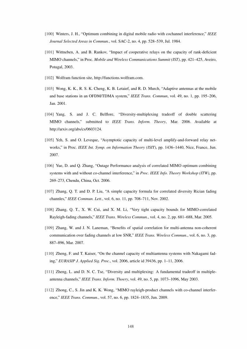
[100] Winters, J. H., “Optimum combining in digital mobile radio with cochannel interference,” IEEE

Journal Selected Areas in Commun., vol. SAC-2, no. 4, pp. 528–539, Jul. 1984.

[101] Wittneben, A. and B. Rankov, “Impact of cooperative relays on the capacity of rank-deficient

MIMO channels,” in Proc. Mobile and Wireless Communications Summit (IST), pp. 421–425, Aveiro,

Potugal, 2003.

[102] Wolfram function site, http://functions.wolfram.com.

[103] Wong, K. K., R. S. K. Cheng, K. B. Letaief, and R. D. Murch, “Adaptive antennas at the mobile

and base stations in an OFDM/TDMA system,” IEEE Trans. Commun, vol. 49, no. 1, pp. 195–206,

Jan. 2001.

[104] Yang, S. and J. C. Belflore, “Diversity-multiplexing tradeoff of double scattering

MIMO channels,” submitted to IEEE Trans. Inform. Theory, Mar. 2006. Available at

http://arxiv.org/abs/cs/0603124.

[105] Yeh, S. and O. Leveque, “Asymptotic capacity of multi-level amplify-and-forward relay net-

works,” in Proc. IEEE Int. Symp. on Information Theory (ISIT), pp. 1436–1440, Nice, France, Jun.

2007.

[106] Yue, D. and Q. Zhang, “Outage Performance analysis of correlated MIMO optimum combining

systems with and without co-channel interference,” in Proc. IEEE Info. Theory Workshop (ITW), pp.

269–273, Chendu, China, Oct. 2006.

[107] Zhang, Q. T. and D. P. Liu, “A simple capacity formula for correlated diversity Rician fading

channles,” IEEE Commun. Lett., vol. 6, no. 11, pp. 708–711, Nov. 2002.

[108] Zhang, Q. T., X. W. Cui, and X. M. Li, “Very tight capacity bounds for MIMO-correlated

Rayleigh-fading channels,” IEEE Trans. Wireless Commun., vol. 4, no. 2, pp. 681–688, Mar. 2005.

[109] Zhang, W. and J. N. Laneman, “Benefits of spatial correlation for multi-antenna non-coherent

communication over fading channels at low SNR,” IEEE Trans. Wireless Commun., vol. 6, no. 3, pp.

887–896, Mar. 2007.

[110] Zheng, F. and T. Kaiser, “On the channel capacity of multiantenna systems with Nakagami fad-

ing,” EURASIP J. Applied Sig. Proc., vol. 2006, article id 39436, pp. 1–11, 2006.

[111] Zheng, L. and D. N. C. Tse, “Diversity and multiplexing: A fundamental tradeoff in multiple-

antenna channels,” IEEE Trans. Inform. Thoery, vol. 49, no. 5, pp. 1073–1096, May 2003.

[112] Zhong, C., S. Jin and K. K. Wong, “MIMO rayleigh-product channels with co-channel interfer-

ence,” IEEE Trans. Commun., vol. 57, no. 6, pp. 1824–1835, Jun. 2009.

148

149