Embed Size (px)
Citation preview
Probabilistic Engineering Analysis Using the NESSUS Software
Ben H. Thackera, David S. Rihaa, Simeon H.K. Fitchb, Luc J. Huysea
aSouthwest Research Institute, 6220 Culebra Road, San Antonio, TX 78228, USA
bMustard Seed Software, San Antonio, TX
ABSTRACT
The development of reliability-based design methods requires the use of general-purpose
engineering analysis tools that predict the uncertainty in a response due to uncertainties in the
model formulation and input parameters. Barriers that have prevented the full acceptance of
probabilistic analysis methods in the engineering design community include availability of tools,
ease of use, robust and accurate probabilistic analysis methods, and the ability to perform
probabilistic analyses for large-scale problems. The goal of the reported work has been to
develop a software tool that fully addresses these three aspects (availability, robustness and
efficiency) to enable the designer to efficiently and accurately account for uncertainties as they
might affect structural reliability and risk assessment. The paper discusses the NESSUS
probabilistic engineering analysis software with specific sections on the reliability modeling and
analysis process in NESSUS, the robust and accurate solution strategies incorporated in the
available probabilistic analysis methods, and several application examples to demonstrate the
applicability of probabilistic analysis to large-scale engineering problems.
Keywords: NESSUS, Probabilistic, Software, Reliability, Uncertainty, Stochastic
1 INTRODUCTION AND BACKGROUND
As performance requirements and testing costs for engineered systems continue to increase,
computational simulation is being increasingly relied upon to serve as a predictive tool. To meet
these requirements, analysts are developing higher fidelity models in an attempt to accurately
1

represent the behavior of the physical system. It is not uncommon nowadays for these models to
involve multiple physics, complex interfaces, and several million finite elements. Despite the
recent extraordinary increase in computer power, analyses performed with these high fidelity
models continue to take hours or even days to complete for a single deterministic analysis.
Structural performance is directly affected by uncertainties associated with models or in physical
parameters and loadings. The traditional design approach has been to adopt safety factors to
ensure that the risk of failure is sufficiently small, albeit not quantified. However, probabilistic
analysis permits a more rigorous quantification of the various uncertainties, and ultimately will
facilitate a more efficient design process. Areas in which probabilistic methods are being
successfully applied include engineered components and systems with high consequences of
failure driven by safety or cost concerns. Some of these areas include aircraft propulsion
systems, airframes, biomechanical systems and prosthetics, nuclear and conventional weapon
systems, space vehicles, pipelines, nuclear waste disposal, offshore structures and automobiles.
In general, probabilistic analysis requires multiple solutions of the underlying (deterministic)
performance model. Consequently, the development of efficient and accurate probabilistic
analysis methods and software tools are critically needed.
Southwest Research Institute (SwRI) has been addressing the need for efficient probabilistic
analysis methods for over twenty years. Much of the reliability technology developed and
implemented by SwRI researchers is available in the NESSUS probabilistic analysis software.
[1] NESSUS (Numerical Evaluation of Stochastic Structures Under Stress) is a general-purpose
tool for computing the probabilistic response or reliability of engineered systems. NESSUS can
be used to simulate uncertainties in loads, geometry, material behavior, and other user-defined
random variables to predict the probabilistic response, reliability and probabilistic sensitivity
measures of engineered systems. The software was originally developed by a team led by SwRI
as part of the NASA project entitled “Probabilistic Structural Analysis Methods (PSAM) for
Select Space Propulsion Components.” [2]
Since the inception of the NASA program, SwRI has continued to conduct research,
development and implementation of probabilistic methods in NESSUS. Through automatic
2

downloads from the NESSUS web site (www.nessus.swri.org), over a thousand copies of the
software have been distributed to a wide range of users around the world. Many of these users
include professors, researchers and students who are incorporating probabilistic design
methodologies into their teaching and research projects. Users from commercial industry and
government are applying NESSUS to a wide range of problems.
NESSUS allows the user to perform probabilistic analysis with analytical models, external
computer programs such as commercial finite element codes, and general combinations of the
two. As an example, consider the problem of estimating the damage to the high-strength steel
used in a containment vessel that confines high explosive experiments. In NESSUS the user can
define a simulation to include 1) an explosive burn calculation to compute the pressure history at
the containment wall boundary, 2) a finite element stress analysis using the computed pressure
history as a load input, and 3) an analytical cumulative damage life calculation based on the
computed stresses. Each model in the simulation can include random variables. This sequentially
linked hierarchy of models allows the user to quickly and easily create complex multi-physics
based probabilistic simulations.
The NESSUS graphical user interface (GUI) is highly configurable and allows tailoring to
specific applications. This GUI provides a capability for commercial or in-house developed
codes to be easily integrated into the NESSUS framework. Eleven probabilistic algorithms are
available in NESSUS including methods such as Monte Carlo simulation, first order reliability
method, advanced mean value method and adaptive importance sampling. [3]
NESSUS is available on a wide variety of computer platforms including Windows (NT, 2000,
XP), IRIX, Solaris, HP-UX and Linux. The user selects the desired platform before downloading
from the NESSUS web site.
Recent work in NESSUS has been based on reducing the time required to define complex
probabilistic problems, improving support for large-scale numerical models (greater than one
million elements), and improving the robustness of the low-level probability integration routines.
In the area of robustness, research is underway to improve most probable point (MPP) search
3
algorithms, develop solution strategies for identifying and solving problems that have multiple
MPP’s, and implement adaptive algorithms that can detect numerical difficulties and
automatically switch to alternative solution strategies. [4,5] Work is also underway to allow
uncertainty due to vague or non-specific input such as expert opinion to also be considered in the
probabilistic analysis. [6,7]
In the following sections, the capabilities and approach to reliability modeling using the
NESSUS software is described. As appropriate, references are made to considerations for large-
scale complex models. Three application problems are presented at the end of the paper to
illustrate the application of NESSUS to real-world problems.
2 OVERVIEW OF NESSUS
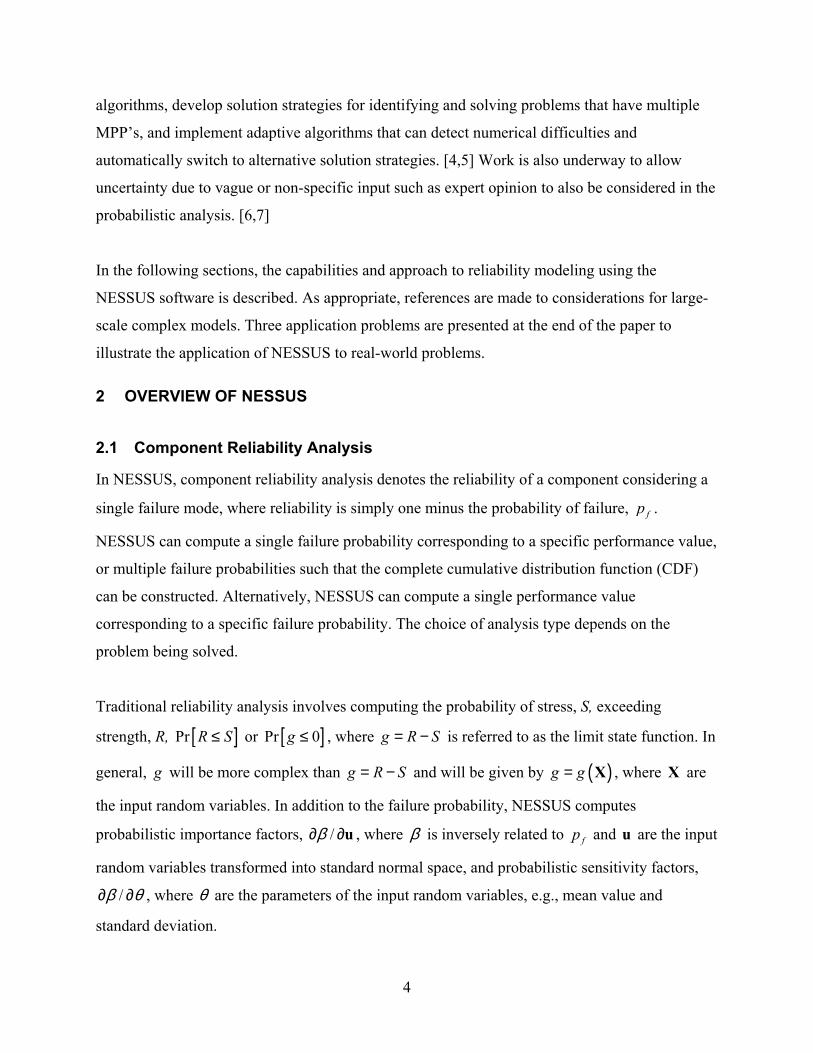
2.1 Component Reliability Analysis
In NESSUS, component reliability analysis denotes the reliability of a component considering a
single failure mode, where reliability is simply one minus the probability of failure, fp .
NESSUS can compute a single failure probability corresponding to a specific performance value,
or multiple failure probabilities such that the complete cumulative distribution function (CDF)
can be constructed. Alternatively, NESSUS can compute a single performance value
corresponding to a specific failure probability. The choice of analysis type depends on the
problem being solved.
Traditional reliability analysis involves computing the probability of stress, S, exceeding
strength, R, [ ]Pr R S≤ or [ ]Pr 0g ≤ , where is referred to as the limit state function. In
general, will be more complex than and will be given by , where are
the input random variables. In addition to the failure probability, NESSUS computes
probabilistic importance factors,
g R S= −
S−g g R= ( )g g= X X
/β∂ ∂u , where β is inversely related to fp and u are the input
random variables transformed into standard normal space, and probabilistic sensitivity factors,
/β θ∂ ∂ , where are the parameters of the input random variables, e.g., mean value and
standard deviation.
θ
4

2.2 System Reliability Analysis
Most engineering structures can fail in more than one way. System reliability considers the
possible failure of multiple components of a system, or multiple failure modes of a component.
In NESSUS, system reliability problems are formulated and solved using a probabilistic fault
tree analysis (PFTA) method. [8]
A fault tree is constructed in NESSUS by connecting “bottom events” with “AND” and “OR”
gates. Each bottom event models a separate failure event, which can be a complex multi-physics
simulation as described earlier in the paper. The topology of the fault tree is defined by the
failure modes being simulated. Once defined, several options are available for solving the system
reliability problem. First, direct Monte Carlo simulation is available but may be cost prohibitive
if the limit state functions of the bottom events are computationally expensive. Alternatively,
NESSUS can compute the probability of system failure using the Advanced Mean Value
(AMV+) method [9] or Adaptive Importance Sampling (AIS) [10]. Because the NESSUS PFTA
uses a limit state function to represent each bottom event, correlations due to common random
variables between the bottom events is fully accounted for regardless of the probabilistic method
used.
In addition to quantifying the system reliability, NESSUS also computes probabilistic
sensitivities of the system probability of failure with respect to the each random variable’s mean
value and standard deviation. [3] These results provide a ranking based on the relative
contribution of each variable to the total probability of failure. The sensitivities are also useful in
design optimization, test planning and resource allocation.
Probabilistic fault trees for system problems are defined in NESSUS using a graphical editor.
Once the system is defined in the GUI, the corresponding Boolean algebraic statement is
transferred to the problem statement window, where the user then defines each event. An
example fault tree and problem statement for a two gate, three-event system is shown in Figure
1.
5

2.3 Reliability Modeling Process
The steps needed to solve a reliability problem in NESSUS include: 1) Develop the functional
relationships that define the model, 2) define the random variable inputs, 3) define the numerical
models needed in the functional relationship, 4) perform parameter variation studies to check and
understand the deterministic behavior of the model, 5) perform the probabilistic analysis, and 6)
visualize the results. NESSUS uses an outline structure to define the problem, as shown in the
left hand side of Figure 2. The user navigates through the nodes of the outline from top to bottom
to define the problem and perform the analysis. Each of these steps is described in more detail in
the following sections.
2.3.1 Problem Statement Definition
The problem statement window in NESSUS is where the functional relationships are entered to
define the model. In the problem statement window, each model is defined only in terms of input
and output variables and mathematical operators. This improves readability, conveys the
essential flow of the analysis, and allows complex reliability assessments to be defined when
more than one model is required to define the system performance.
An example problem statement is shown in the upper right hand portion of Figure 2. A powerful
feature of NESSUS is the ability to create complex probabilistic simulations by linking models
together in a sequential fashion. In this example, the performance measure is life (given by
number of cycles to failure), which requires input from other models. Two stress quantities from
an ABAQUS (ABAQUS, Inc.) finite element analysis are used in the analytical life model. Many
other finite element codes are interfaced with NESSUS and will be described in a subsequent
section. Finally, the ABAQUS model requires input from several independent variables. The
problem statement parser in NESSUS identifies all of the independent variables in the problem
statement window and transfers these variables to the random variable input window for further
definition.
2.3.2 Random Variable Input and Probabilistic Database
The random variable inputs are defined in the random variable definition window in NESSUS. A
graphical input editor is provided for distributions requiring parameters other than the mean and
standard deviation, such as upper and lower bounds for truncated distributions. The probability
6

density function (PDF) and cumulative distribution function (CDF) plotting capability in
NESSUS provides a quick visual inspection of the random variables. Random variables allowed
in NESSUS include normal, lognormal, Weibull, extreme value type I, chi-square, maximum
entropy, curve-fit, Frechet, truncated normal and truncated Weibull. The maximum entropy and
curve-fit distributions can be used for distributions not directly supported.
NESSUS maintains a library of relevant PDFs in a probabilistic database. Random variables can
be defined and stored using a distribution type and associated parameters. Distribution fitting
functions are provided to determine the best fit from raw data. The entries can be grouped and
multiple databases are supported. This allows users to develop their own, possibly proprietary,
databases for use in NESSUS. Random variable definitions from the database contents can be
inserted directly in the random definition table in NESSUS using a right mouse click as shown in
Figure 3.
2.3.3 Response Model Definition
Functions defined in the problem statement window (Figure 2) are assigned in the response
model definition. The available function types are selected from the model type drop down menu
and include analytical, regression, numerical, and predefined as shown in Figure 4. The
analytical function type allows models to be defined with standard mathematical operators, using
a format identical to definitions in the problem statement window. The numerical model type
allows the use of interfaced codes or a user-defined code. Codes currently interfaced to NESSUS
include ABAQUS, ANSYS (ANSYS, Inc.), DYNA3D (Lawrence Livermore National
Laboratory), LS-DYNA (LSTC, Inc.), NASA_GRC_FEM (NASA Glenn Research Center),
MADYMO (TNO Automotive), MSC.NASTRAN (MSC.Software), PRONTO (Sandia National
Laboratories), and USER_DEFINED. The regression model type allows the user to input
function coefficients or raw perturbation data that can be fit to linear or quadratic functions using
linear regression. Finally, the predefined model type allows linking user-written Fortran
subroutines with NESSUS, which requires the user to have access to a Fortran compiler. The
user-defined numerical model allows the user to link the NESSUS probabilistic engine with any
stand-alone analysis code.
7

Figure 4 shows an example using the ABAQUS finite element program. The execution command
window provides the command or commands required to execute ABAQUS. The input and
output files are also defined on this input screen. Default execution options for the supported
codes are inserted automatically by NESSUS from a configurable template file, and can be
modified by the user as needed.
A batch processing option is provided to allow processing on different computers. This allows
NESSUS to run on a local workstation while the analysis codes run on a different workstation,
cluster, supercomputer, etc. Related to the batch processing feature, NESSUS also provides an
automatic restart option. The restart capability provides probabilistic solution refinement,
recovering from abnormal solver termination, and evaluating additional performance measures
without rerunning previous steps of the solver analyses.
2.3.3.1 Mapping Random Variables to Numerical Models
When performing probabilistic analysis using a numerical model, a realization of a random
variable must be reflected in the numerical model’s input. The variable may be a random
variable or a computed variable from another code or analytical equation. In general, the variable
can map to a single value in the code’s input or to a vector of values such as nodal coordinates in
a finite element model. Typical examples of single value mappings include Young's modulus or
a concentrated point load. Examples of vector mappings are a pressure field acting on a set of
elements or a geometric parameter that effects multiple node locations.
Mapping variables to the numerical model input in NESSUS is achieved by graphically
identifying the lines and columns that are changed when the variable changes as shown in Figure
5. The visual feedback of the mapping between the random variable and the finite element input
greatly reduce the chance for error. The mapping capability in NESSUS has been optimized to
support model input files in excess of several million lines in length.
Vector mappings require a functional relationship between the input random variable and the
analysis program input. Because different realizations of these variables are required, a general
approach is used in NESSUS to relate a change in the input random variable value to the code’s
8
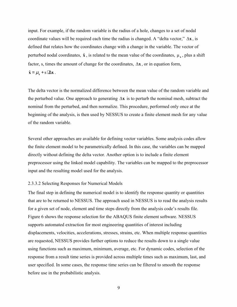
input. For example, if the random variable is the radius of a hole, changes to a set of nodal
coordinate values will be required each time the radius is changed. A “delta vector,” ∆ , is
defined that relates how the coordinates change with a change in the variable. The vector of
perturbed nodal coordinates, x , is related to the mean value of the coordinates, , plus a shift
factor, s, times the amount of change for the coordinates, ∆ , or in equation form,
x
ˆ xµ
x
ˆ sµ= + ⋅∆xx x .
The delta vector is the normalized difference between the mean value of the random variable and
the perturbed value. One approach to generating is to perturb the nominal mesh, subtract the
nominal from the perturbed, and then normalize. This procedure, performed only once at the
beginning of the analysis, is then used by NESSUS to create a finite element mesh for any value
of the random variable.
x∆
Several other approaches are available for defining vector variables. Some analysis codes allow
the finite element model to be parametrically defined. In this case, the variables can be mapped
directly without defining the delta vector. Another option is to include a finite element
preprocessor using the linked model capability. The variables can be mapped to the preprocessor
input and the resulting model used for the analysis.
2.3.3.2 Selecting Responses for Numerical Models
The final step in defining the numerical model is to identify the response quantity or quantities
that are to be returned to NESSUS. The approach used in NESSUS is to read the analysis results
for a given set of node, element and time steps directly from the analysis code’s results file.
Figure 6 shows the response selection for the ABAQUS finite element software. NESSUS
supports automated extraction for most engineering quantities of interest including
displacements, velocities, accelerations, stresses, strains, etc. When multiple response quantities
are requested, NESSUS provides further options to reduce the results down to a single value
using functions such as maximum, minimum, average, etc. For dynamic codes, selection of the
response from a result time series is provided across multiple times such as maximum, last, and
user specified. In some cases, the response time series can be filtered to smooth the response
before use in the probabilistic analysis.
9

A flexible user defined numerical model capability is provided in NESSUS. This capability
allows users to link in-house developed codes with NESSUS. The response of interest is selected
by defining a specific location in the analysis code’s results file. A user subroutine for extracting
responses is also available for more complex situations such as results extraction from a binary
database file.
2.3.4 Deterministic and Parameter Variation Analysis
NESSUS’ deterministic analysis option provides a useful tool to verify the problem statement
definition. Any computed value (on the left of the equal sign) in the problem statement will be
evaluated at the mean values of the input random variables.
Parameter variation analysis is another useful tool to understand how the performance varies
with changes in the random variables. NESSUS provides several methods for defining variable
perturbations including, backward, central, and forward differences as well as variable sweeps.
In addition, specific perturbation values can be input directly to define experimental designs.
Visualization of the response variation is provided in predefined XY scatter plots.
2.3.5 Probabilistic Analysis Definitions
Many efficient probabilistic analysis methods have been devised to alleviate the need for Monte
Carlo simulation, which is impractical for large-scale high-fidelity problems. [11] The traditional
methods include, for example, the first and second-order reliability methods (FORM and SORM)
[12], the response surface method (RSM) [13], and Latin hypercube simulation (LHS) [14].
Methods tailored for complex probabilistic finite element analysis include, for example, the
advanced mean value family of methods (AMV+) [9] and adaptive importance sampling (AIS).
[10] Further details on these methods and their implementation in NESSUS are given in Ref. [3].
NESSUS has a suite of probabilistic analysis methods as listed in Table 1 for both component
and system probabilistic analysis. The range of methods allows the analyst to obtain probabilistic
solutions with different levels of fidelity based on the requirements of the analysis. NESSUS
provides complete control of each of the available probabilistic methods. As an example, Figure
7 shows the probabilistic analysis definition screen for the AMV+ method. Default parameters
10

for the different methods are supplied based on experience with the method on previous
problems.
In addition to defining the probabilistic method, several other options can be selected: parameter
correlations, confidence bounds, and analysis type. Linear correlation between any two input
variables is defined by entering the correlation coefficient. By default the input variables are
assumed to be statistically independent, i.e., zero correlation. If any non-zero correlations are
entered, NESSUS will perform a numerical transformation during the probability integration to
account for the correlation. NESSUS computes confidence bounds on the computed probabilities
from statistical uncertainty on the mean or standard deviation of each input random variable. To
define statistical uncertainty, the user enters a coefficient of variation (COV) on the mean and
standard deviation for each of the input random variables. All COV values are zero by default.
The analysis type definition indicates that the probabilistic method will compute 1) the full CDF
of the response, 2) the probability associated with a specified performance or list of performance
values, or 3) the performance given a specified probability or set of probability values.
2.3.6 Results Visualization
NESSUS includes a powerful post processing capability. After completing the probabilistic
analysis, the user can visualize the CDF in several formats (Figure 8). In addition, the various
probabilistic sensitivity measures computed by NESSUS can be viewed as shown in Figure 8.
Multiple analyses can be compared on a single plot as a means of comparing different analysis
methods (e.g., Monte Carlo and AMV+) or random variable changes (design “what-if” analyses).
Finally, the user has control over all plot formats such as line styles, titles, and number format.
All plots are easily exported for inclusion in reports or presentations.
Three-dimensional model viewing with color probability contouring is another highly useful
visualization output of NESSUS. The failure probability is computed at different locations in the
model (e.g. all of some of the nodes in a finite element mesh) and visualized by contouring iso-
probability values. Contours of probability can reveal regions of high risk that may not be
apparent from the contours of model response quantities. Consider the spatial thickness
fluctuations of a part induced by the rolling or stamping process. Figure 9 shows that even
11

though the mean stress at point B is higher than at point A, the probability of failure is lower due
to the larger uncertainty at point A.
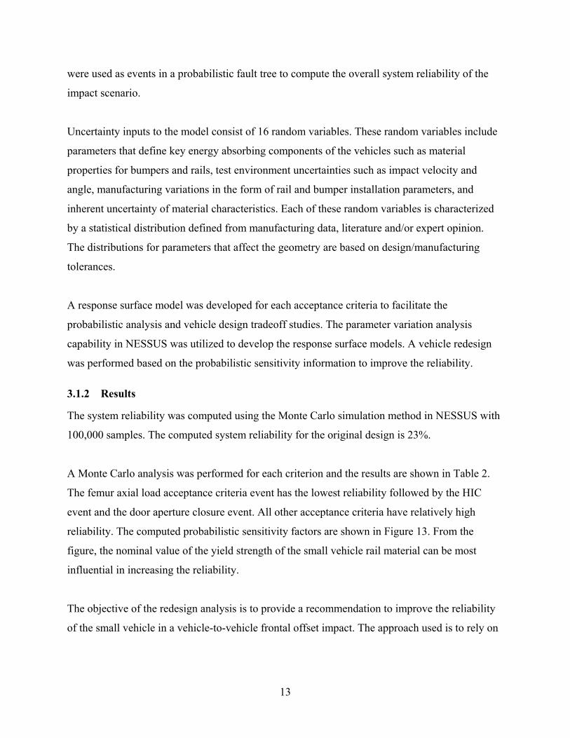
An example of a large-scale analysis utilizing probability contouring is shown in Figure 10. The
probability contours identify regions where there is significant probability that the equivalent
plastic strain exceeds the design limit. As shown, these high-probability regions are not
identified by the equivalent plastic strain contours.
3 APPLICATION EXAMPLES
The NESSUS software has been used to predict the reliability and probabilistic response for a
wide range of problems. [15-23] Three problems are presented in this section to demonstrate the
application and flexibility of NESSUS and to illustrate the current developments to support
efficient probabilistic model development and support for large-scale problems.
3.1 Stochastic Crashworthiness
The NESSUS probabilistic analysis software was used to compute the system reliability of a
Sport utility vehicle to small vehicle frontal offset impact event. The analysis was designed to
identify important variables contributing to the crashworthiness reliability and use this
information to improve the design and manufacturing processes. The ultimate goal of the
analysis is to improve vehicle reliability using a computational approach to reduce expensive
crash testing. Additional details about this analysis can be found in Ref. [24].
3.1.1 Problem Description
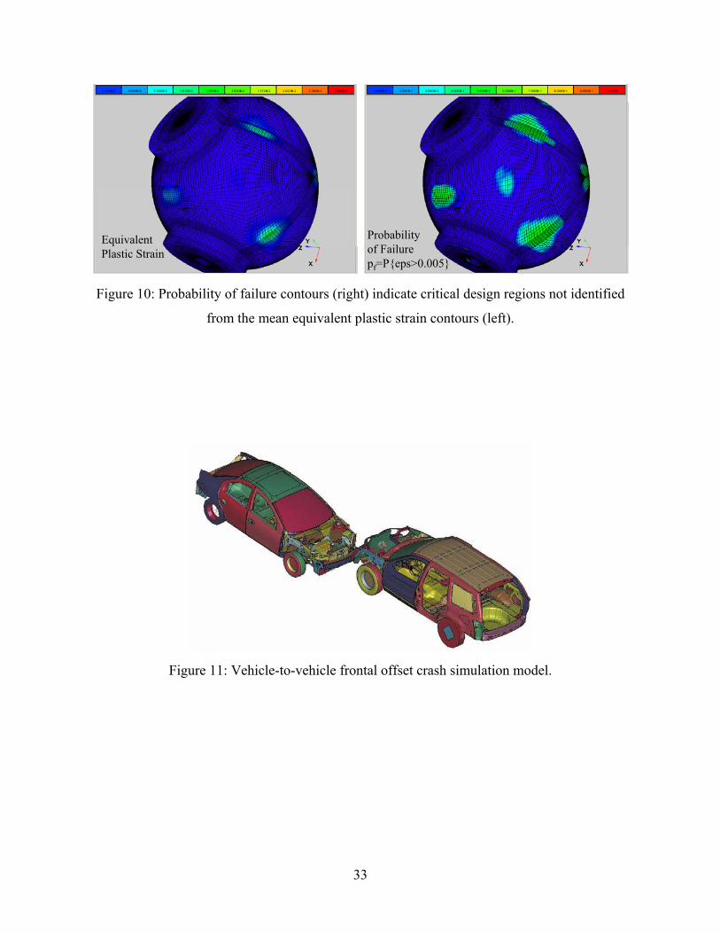
An LS-DYNA finite element model of a vehicle frontal offset impact and a MADYMO model of
a 50th percentile male Hybrid III dummy were integrated with NESSUS to comprise the
crashworthiness characteristics (Figure 11). A number of different response quantities from the
models were used to define four occupant injury acceptance criteria and six compartment
intrusion criteria. The NESSUS problem statement for the Head Injury Criteria (HIC) is shown
in Figure 12. An acceleration history from the LS-DYNA vehicle model is used as the crash
pulse input to the occupant injury model in MADYMO. The other three occupant injury criteria
are modeled in the same fashion. The compartment intrusion criteria are determined from
relative displacements of the points in the small vehicle model. These ten acceptance criteria
12
were used as events in a probabilistic fault tree to compute the overall system reliability of the
impact scenario.
Uncertainty inputs to the model consist of 16 random variables. These random variables include
parameters that define key energy absorbing components of the vehicles such as material
properties for bumpers and rails, test environment uncertainties such as impact velocity and
angle, manufacturing variations in the form of rail and bumper installation parameters, and
inherent uncertainty of material characteristics. Each of these random variables is characterized
by a statistical distribution defined from manufacturing data, literature and/or expert opinion.
The distributions for parameters that affect the geometry are based on design/manufacturing
tolerances.
A response surface model was developed for each acceptance criteria to facilitate the
probabilistic analysis and vehicle design tradeoff studies. The parameter variation analysis
capability in NESSUS was utilized to develop the response surface models. A vehicle redesign
was performed based on the probabilistic sensitivity information to improve the reliability.
3.1.2 Results
The system reliability was computed using the Monte Carlo simulation method in NESSUS with
100,000 samples. The computed system reliability for the original design is 23%.
A Monte Carlo analysis was performed for each criterion and the results are shown in Table 2.
The femur axial load acceptance criteria event has the lowest reliability followed by the HIC
event and the door aperture closure event. All other acceptance criteria have relatively high
reliability. The computed probabilistic sensitivity factors are shown in Figure 13. From the
figure, the nominal value of the yield strength of the small vehicle rail material can be most
influential in increasing the reliability.
The objective of the redesign analysis is to provide a recommendation to improve the reliability
of the small vehicle in a vehicle-to-vehicle frontal offset impact. The approach used is to rely on
13

the probabilistic sensitivity factors to identify the dominant parameters (random variable mean
and standard deviation) that will improve system reliability.
The reliability for each acceptance criteria in the new design is listed in Table 2. The dominant
event for the original design was the femur axial load acceptance criteria. The femur axial load
also shows the lowest reliability for the final design but increased from a reliability of 46% to
93%. The reliability improvements are shown in Figure 14 along with a description of the
parameter changes to achieve the improvement. The system reliability for the final design is
86%.
A system reliability analysis is critical to the correct evaluation of the vehicle performance
especially for evaluating the probabilistic sensitivity factors at the system level for redesign
analysis. Certain parameters such as stiffness/strength parameters can improve reliability for
compartment intrusion performance measures but may be detrimental to the crash pulse
attenuated to the vehicle occupant. The system model correctly accounts for events with common
variables (correlated events) and thus correctly identifies the important variables on the system
level.
3.2 Blast Containment Vessel
Over the past 30 years, Los Alamos National Laboratory (LANL), under the auspices of DOE,
has been conducting confined high explosion experiments utilizing large, spherical, steel
pressure vessels. These experiments are performed in a containment vessel to prevent the release
of explosion products to the environment. Design of these spherical vessels was originally
accomplished by maintaining that the vessel’s kinetic energy, developed from the detonation
impulse loading, be equilibrated by the elastic strain energy inherent in the vessel. Within the last
decade, designs have been accomplished utilizing sophisticated and advanced 3D computer
codes that address both the detonation hydrodynamics and the vessel’s highly nonlinear
structural response. Additional details about this analysis can be found in Refs. [22,25].
3.2.1 Problem Description
The containment vessel, shown on the left side in Figure 15, is a spherical vessel with three
access ports: two 16-inch ports aligned in one axis on the sides of the vessel and a single 22-inch
14

port at the top of the vessel. The vessel has an inside diameter of 72 inches and a 2 inch nominal
wall thickness. The vessel is fabricated from HSLA-100 steel, chosen for its high strength, high
fracture toughness, and no requirement for post weld heat treatment. The vessel’s three ports
must maintain a seal during use to prevent any release of reaction product gases or material to
the external environment. Each door is connected to the vessel with 64 high strength bolts, and
four separate seals at each door ensure a positive pressure seal.
A series of hydrodynamic and structural analyses of the spherical containment vessel were
performed using a combination of two numerical techniques. Using an uncoupled approach, the
transient pressures acting on the inner surface of the vessel were computed using the Eulerian
hydrodynamics code, CTH (Sandia National Laboratories), which simulated the high explosive
(HE) burn, the internal gas dynamics, and shock wave propagation. The HE was modeled as
spherically symmetric with the initiating burn taking place at the center of the sphere. The
vessel’s structural response to these pressures was then analyzed using the DYNA3D explicit
finite element structural dynamics code.
The simulation required the use of a large, detailed mesh to accurately represent the dynamic
response of the vessel and to adequately resolve the stresses and discontinuities caused by
various engineering features such as the bolts connecting the doors to their nozzles. Taking
advantage of two planes of symmetry, one quarter of the structure was meshed using
approximately one million hex elements. Six hex elements were used through the 2-inch wall
thickness to accurately simulate the bending behavior of the vessel wall. The one-quarter
symmetry model is shown on the right hand side of Figure 15. The structural response simulation
used an explicit finite element code called PARADYN (Lawrence Livermore National
Laboratory), which is a massively parallel version of DYNA3D, a nonlinear, explicit Lagrangian
finite element analysis code for three-dimensional transient structural mechanics. PARADYN
was run on 504 processors of LANL’s “Blue Mountain,” massively parallel computer, which is
an interconnected array of independent SGI (Silicon Graphics, Inc.) computers. The containment
vessel model can be solved on the Blue Mountain computer with approximately 2.5 hours of run
time. The same analysis would have taken about 35 days when run on a single processor.
15

The four random variables considered are radius of the vessel wall (radius), thickness of the
vessel wall (thickness), modulus of elasticity (E), and yield stress (Sy) of the HSLA steel. A
summary of the probabilistic inputs is included in Table 3. The properties for radius and
thickness are based on a series of quality control inspection tests that were performed by the
vessel manufacturer. The coefficients of variation for the material properties are based on
engineering judgment. In this case, the material of the entire vessel, excluding the bolts, is taken
to be a random variable.
When the thickness and radius random variables are perturbed, the nodal coordinates of the finite
element model change with the exception of the three access ports in the vessel, which remain
constant in size and move only to accommodate the changing wall dimensions. This was
accomplished in NESSUS by defining a set of scale factors that defined how much and in what
direction each nodal coordinate was to move for a given perturbation in both thickness and
radius. The NESSUS mapping procedure allows the perturbations in radius and thickness to be
cumulative so these variables can be perturbed simultaneously. Once the scale factors are defined
and input to NESSUS, the probabilistic analysis, whether by simulation or using AMV+, can be
performed without further user intervention.
The response metric for the probabilistic analysis is the maximum equivalent plastic strain
occurring over all times at the bottom of the vessel finite element model. This maximum value
occurred well after the initial pulse and was caused by bending modes created by the ports.
3.2.2 Results
The AMV+ method in NESSUS was used to calculate the CDF of equivalent plastic strain. Also,
LHS was performed with 100 samples to verify the correctness of the AMV+ solution near the
mean value. The CDF is plotted on the left in Figure 16 on a standard normal probability scale.
As shown, the LHS and AMV+ results are in excellent agreement. However, in contrast to the
LHS solution, the AMV+ solution predicts accurate probabilities in the extreme tail regions with
far fewer PARADYN model evaluations.
Probabilistic sensitivities are shown in on the right in Figure 16. The sensitivities are multiplied
by to nondimensionalize the values and facilitate a relative comparison between parameters. iσ
16

The values are also normalized such that the maximum value is equal to one. It can be concluded
that the reliability is most sensitive to the mean and standard deviation of the thickness of the
containment vessel wall.
3.3 Cervical Spine Impact Injury
Cervical spine injuries occur as a result of impact or from large inertial forces such as those
experienced by military pilots during ejections, carrier landings, and ditchings. Other examples
include motor vehicle, diving, and athletic-related accidents. Reducing the likelihood of injury
by identifying and understanding the primary injury mechanisms and the important factors
leading to injury motivates research in this area. [26]
Because of the severity associated with most cervical spine injuries, it is of great interest to
design occupant safety systems to minimize probability of injury. To do this, the designer must
have quantified knowledge of the probability of injury due to different impact scenarios, and also
know which model parameters contribute the most to the injury probability. Finite element stress
analysis plays a critical role in understanding the mechanics of injury and the effects of
degeneration as a result of disease on the structural performance of spinal segments. However, in
many structural systems, there is a great deal of uncertainty associated with the environment in
which the structure is required to function. This variability or uncertainty has a direct effect on
the structural response of the system. Biological systems are a textbook example: uncertainty and
variability exist in the physical and mechanical properties and geometry of the bone, ligaments,
cartilage, as well as uncertainty in joint and muscle loads. Hence, the broad objective of this
investigation is to explore how uncertainties influence the performance of an anatomically
accurate, three-dimensional, non-linear, experimentally validated finite element model of the
human lower cervical spine.
3.3.1 Problem Description
A validated three-dimensional ABAQUS finite element model of the C4-C5-C6 spinal segment
developed at the Medical College of Wisconsin [27] was used to calculate the structural response
of the lower cervical spine and to quantify the effect of uncertainties on the performance of the
biological system. The load-deflection response was validated against experimental results from
eight cadaver specimens [28]. The moment–rotation response of the finite element model was
17

validated against experimental results reported in the literature [29]. The model is shown in
Figure 17. Additional details about this analysis can be found in Ref. [30].
Biological variability was accounted for by modeling material properties and spinal segment
loading as random variables. Where available, experimental data was used to generate the
random variable definitions (e.g. the spinal ligaments load-deflection behavior).
The probabilistic finite element model was exercised under flexion (chin down) loading by
applying a pure bending moment of 2 N-m to the superior surface of the C4 vertebra. The
inferior surface of the C6 vertebra was fixed in all directions and rotation was measured between
the superior aspect of C4 and the fixed boundary of C6. Computing the rotation and monitoring
the reaction forces at the fixed boundary quantified the moment-rotation behavior. Cumulative
probability distribution functions, probability distribution functions, and probabilistic sensitivity
factors were determined.
The random variables considered in the analysis are given in Table 4. The mean values were set
equal to the nominal values used in Ref. [27]. Thus, the original deterministic solution will be
obtained when the random variables are set equal to their mean values. Since data were not
available to characterize all of the model inputs, it was decided to model all random variables
with a coefficient of variation of ten percent. Default distributions were assigned based on
experience, i.e., a lognormal distribution was used to model modulus variables and a normal
distribution was used otherwise.
3.3.2 Results
Probabilistic results were computed using the coupled NESSUS – ABAQUS model and the
AMV+ probabilistic method. In the analysis, 41 function (ABAQUS) evaluations were required.
The probabilistic rotation response had an approximate mean of 3.82 degrees and a standard
deviation of 0.38 degrees resulting in a coefficient of variation of 10%. The CDF and PDF of
rotation is shown on the left in Figure 18. The CDF is used to determine probabilities directly,
e.g., the probability that the rotation will be less than or equal to 4.2o is 82%.
18

The probabilistic sensitivity factors indicate that the loading (FLEXLOAD) is the dominant
variable. The bar graph on the right in Figure 18 shows the sensitivity information for the eight
most significant random variables with FLEXLOAD removed so that the other variables can be
more clearly seen. Not including FLEXLOAD, the most important variables are the: 1) annulus
C45 and C56 Young’s modulus, 2) interspinous ligament nonlinear spring force-deflection
relationship, and 3) ligamentum flavum nonlinear spring force-deflection relationship. These
results can be used eliminate unimportant variables from the random variable vector and to focus
further characterization efforts on those variables that are most significant.
4 CONCLUSIONS
Although NESSUS was initially developed for aerospace applications, the methods are broadly
applicable and their use warranted in situations where uncertainty is known or believed to have a
significant impact on the structural response. The framework of NESSUS allows the user to link
advanced probabilistic algorithms with analytical equations, commercial finite element analysis
programs and “in-house” stand-alone deterministic analysis codes to compute the probabilistic
response or reliability of a system.
For probabilistic methods to be accepted for use in design, probabilistic tools must be robust,
easy to use, and interfaced with widely used commercial analysis packages. This integration with
commercially available analysis software leverages the investment made in learning and
becoming proficient with the software. The graphical user interface in NESSUS makes defining
and executing the probabilistic analysis straightforward and efficient for simple problems as well
as problems involving extremely large multi-physics models.
Several applications were presented that demonstrated the flexibility of the NESSUS software.
The advanced probabilistic analysis methods in NESSUS allow for using high-fidelity models to
define the structure or system even when each function evaluation may take several hours to run.
In the application problems presented, the probabilistic results revealed additional information
that would not have been available if deterministic approaches were used.
19

Future progress in probabilistic mechanics relies strongly on the development of validated
analysis models, systematic data collection and synthesis to resolve probabilistic inputs, and
identification and classification of failure modes. Research and development in this area is
needed to improve the robustness of the underlying probability integration methods, to develop
alternative uncertainty modeling approaches and integrate these approaches with established
probabilistic tools, and to apply probabilistic methods to model verification and validation,
system certification and prognosis, component life assessment and integrity, and structural
system health monitoring and management.
5 ACKNOWLEDGEMENTS
The authors wish to acknowledge the support of the NASA Glenn Research Center and the Los
Alamos National Laboratory for their significant support of the NESSUS software. The 2000
DaimlerChrysler Challenge Fund, Naval Air Warfare Center Aircraft Division, and Los Alamos
National Laboratory are also acknowledged for their support for the applications problems
summarized in the paper.
6 REFERENCES
1. NESSUS User’s manual, Version 8, Southwest Research Institute, www.nessus.swri.org,
2004.
2. Southwest Research Institute, “Probabilistic Structural Analysis Methods (PSAM) for Select
Space Propulsion System Components,” Final Report NASA Contract NAS3-24389, NASA
Lewis Research Center, Cleveland, Ohio, 1995.
3. NESSUS Theory manual, Version 8, Southwest Research Institute, 2004.
4. Thacker, B.H., Riha, D.S., Millwater, H.R., Enright, M.P., “Errors and Uncertainties in
Probabilistic Engineering Analysis,” Proceedings AIAA/ASME/ASCE/AHS/ASC 42nd
Structures, Structural Dynamics, and Materials (SDM) Conference, AIAA 2001-1239,
Seattle, WA, 16-19 April 2001.
5. Riha, D.S., Thacker, B.H.,Fitch, S.H.K “NESSUS Capabilities for Ill-Behaved Performance
Functions,” Proceedings AIAA/ASME/ASCE/AHS/ASC 45th Structures, Structural
Dynamics, and Materials (SDM) Conference, AIAA 2004-1832, Palm Springs, CA, 19-22
April 2004.
20

6. Huyse, L. and B.H. Thacker, “Treatment of Conflicting Expert Opinion in Probabilistic
Analysis,” Proc. 11th IFIP WG7.5 Working Conference on Reliability and Optimization of
Structural Systems, M.A. Maes and L. Huyse, Eds, A.A. Balkema Publishers, Banff, Canada,
November 2003.
7. Thacker, B.H. and L. Huyse, A Framework to Estimate Uncertain Random Variables, AIAA
Paper 2004-1828, 45th AIAA/ASME/ASCE/AHS/ ASC Structures, Structural Dynamics and
Materials Conference, 2004.
8. Torng, T.Y., Wu, Y.-T., and Millwater, H.R., "Structural System Reliability Calculation
Using a Probabilistic Fault Tree Analysis Method," Proc. 33rd
AIAA/ASME/ASCE/AHS/ASC Structures, Structural Dynamics, and Materials Conf., Paper
No. AIAA-92-2410, Dallas, TX, April 13-15, 1992.
9. Wu, Y.-T., H. R. Millwater, and T. A. Cruse, “Advanced Probabilistic Structural Analysis
Methods for Implicit Performance Functions,” AIAA Journal, 28(9), 1990.
10. Wu, Y.-T., “Computational Method for Efficient Structural Reliability and Reliability
Sensitivity Analysis,” AIAA Journal, Vol. 32, 1994.
11. Ang, A. H.-S. and Tang, W. H., Probabilistic Concepts in Engineering Planning and Design,
Volume II: Decision, Risk, and Reliability, New York: John Wiley & Sons, Inc., 1984.
12. Madsen, H. O., Krenk, S., and Lind, N. C., Methods of Structural Safety, Prentice-Hall, Inc.,
New Jersey, 1986
13. Faravelli, L., “Response Surface Approach for Reliability Analysis,” J. of Eng. Mech.,
115(12), 1989.
14. McKay, M.D. and R.J. Beckman, 1979, “A Comparison of Three Methods for Selecting
Values of Input Variables in the Analysis of Output From a Computer Code.”
Technometrics, Vol. 21, No. 2, pp. 239-245.
15. Riha, D.S., B.H. Thacker, D.A. Hall, T.R. Auel, and S.D. Pritchard, “Capabilities and
Applications of Probabilistic Methods in Finite Element Analysis,” Int. J. of Materials &
Product Technology, Vol. 16, Nos. 4/5, 2001.
16. Millwater, H., Griffin, K., Wieland, D., West, A., Smith, H., Holly, M., and Holzwarth, R.,
“Probabilistic Analysis of an Advanced Fighter/Attack Composite Wing Structure,” Proc.
41st AIAA/ASME/ASCE/AHS/ASC Structures, Structural Dynamics, and Materials Conf.,
Paper No. 2000-1567, Atlanta, GA, April 3-6, 2000.
21

17. Shah, C.R., Sui, P., Wang, W., and Wu, Y.-T., "Probabilistic Reliability Analysis of an
Engine Crankshaft," Proceedings 8th Int. ANSYS Conf., August 1998.
18. Thacker, B.H., Oswald, C.J., Wu, Y.-T., Patterson, B.C., Senseny, P.E., and Riha, D.S., "A
Probabilistic Multi-Mode Damage Model for Tunnel Vulnerability Assessment," Proc. 8th
Annual Symposium on the Interaction of the Effects of Munitions with Structures, Volume
II, pg. 137-148, McClean, VA, April 22-25, 1997.
19. Millwater, H. R. and Wu, Y.-T., 1993, “Computational Structural Reliability Analysis of a
Turbine Blade,” Proc. of the International Gas Turbine And Aeroengine Congress and
Exposition, Cincinnati, OH, May 24-27.
20. Thacker, B. H., Wu, Y.-T., Nicolella, D. P. and Anderson, R. C., "Probabilistic Injury
Analysis of the Cervical Spine," Proc. AIAA/ASME/ASCE/AHS/ASC 38th Structures,
Structural Dynamics, and Materials (SDM) Conf., AIAA 97-1135, Kissimmee, Florida, 7-10
April 1997.
21. Thacker, B.H., Rodriguez, E.A., Pepin, J.E., Riha, D.S., “Application of Probabilistic
Methods to Weapon Reliability Assessment,” Proc. AIAA/ASME/ASCE/AHS/ASC 42nd
Structures, Structural Dynamics, and Materials (SDM) Conference, AIAA 2001-1458,
Seattle, WA, 16-19 April 2001.
22. Rodriguez, E.A., Pepin, J.W., Thacker, B.H., Riha, D.S., “Uncertainty Quantification of A
Containment Vessel Dynamic Response Subjected to High-Explosive Detonation Impulse
Loading”, Proc. AIAA/ASME/ASCE/AHS/ASC 43rd Structures, Structural Dynamics, and
Materials (SDM) Conference, AIAA 2002-1567, Denver, CO, April 2002.
23. Pepin, J.E., Thacker, B.H., Rodriguez, E.A., Riha, D.S., “A Probabilistic Analysis of a
Nonlinear Structure Using Random Fields to Quantify Geometric Shape Uncertainties”, Proc.
AIAA/ASME/ASCE/AHS/ASC 43rd Structures, Structural Dynamics, and Materials (SDM)
Conference, AIAA 2002-1641, Denver, CO, April 2002.
24. Riha, D.S., Hassan, J.E., Forrest, M.D., Ding, K., “Stochastic Approach for Vehicle Crash
Models,” Proc. SAE 2004 World Congress & Exhibition, 2003-01-0460, Detroit, MI., March
2004.
25. Thacker, B.H., Rodriguez, E.A., Pepin, J.E., Riha, D.S., “Uncertainty Quantification of a
Containment Vessel Dynamic Response Subjected to High-Explosive Detonation Impulse
22

Loading,” IMAC-XXI: Conference & Exposition on Structural Dynamics, No. 261,
Kissimmee, FL, 3-6 February 2003.
26. Thacker, B.H., Y.-T. Wu, and Nicolella, D.P., Frontiers in Head and Neck Trauma: Clinical
and Biomechanical, Probabilistic Model of Neck Injury, N. Yoganandan, F.A. Pintar, S.J.
Larson and A. Sances, Jr. (eds.), IOS Press, Harvard, MA, 1998.
27. Kumaresan, S., Yoganandan, N., Pintar, F.A., and Maiman D., “Finite Element Modeling of
the Lower Cervical Spine; Role of Intervertebral Disc under Axial and Eccentric Loads,”
Medical Engineering and Physics, Vol. 21, pp. 689-700, 2000.
28. Pintar, F.A., Yoganandan, N., Pesigan, M., Reinartz, J.M., Sances, A., and Cusik, J.F.,
“Cervical vertebral strain measurements under axial and eccentric loading,” ASME Journal
of Biomechanical Engineering, Vol. 117, pp. 474-478, 1995.
29. Shea, M., Edwards, W.T., White, A.A., and Hayes, W.C., “Variations of stiffness and
strength along the human cervical spine,” Journal of Biomechanics, Vol. 24(2) pp. 95-107,
1991.
30. Thacker, B.H., D. P. Nicolella, S. Kumaresan, N. Yoganandan, F. A. Pintar, “Probabilistic
Finite Element Analysis of the Human Lower Cervical Spine,” Math. Modeling and Sci.
Computing, Vol. 13, No. 1-2, pp. 12-21, 2001.
23

Table 1: Probabilistic analysis methods in NESSUS.
Probabilistic Method Component System First order reliability method (FORM) X Advance first order reliability method X Second order reliability method (SORM) X Importance sampling with radius reduction factor X X Monte Carlo simulation X X Importance sampling with user-defined radius X Plane-based adaptive importance sampling X Curvature-based adaptive importance sampling X X Mean value X Advanced mean value X Advanced mean value with iterations X Latin hypercube simulation X Response surface method with Monte Carlo simulation X
Table 2: Original and final design reliability for the stochastic car crash example.
Acceptance Criteria Reliability Description NESSUS Variable Original Design Final Design
HIC g_hic 57.7910% 94.0120% Chest acceleration g_cg 92.2970% 98.8240% Chest deflection g_chestd 99.9752% 99.9999% Femur axial load g_femurl 46.4020% 92.9330% Footrest intrusion g_fri 99.9623% 100.0000%
Toepan deflection g_tpd 100.0000% 100.0000%
Brake pedal location g_bpd 100.0000% 100.0000%
Instrument panel def. g_ipd 99.6870% 99.9719%
Door aperture closure g_dac 72.6750% 98.7460%
Engine location g_engd 99.6000% 99.9997%
Table 3: Probabilistic inputs for the containment vessel example problem.
Variable PDF σ µ COV Radius (in) Normal 37.0 0.0521 0.00141 Thick (in) Lognormal 2.0 0.08667 0.04333 E (lb/in2) Lognormal 29.0E+06 1.0E+06 0.03448 Sy (lb/in2) Normal 106.0E+03 4.0E+03 0.03774
24

Table 4: Probabilistic inputs for the cervical spine impact injury example problem.
Name Description Mean Standard Deviation Distribution
MALLRV Anterior longitudinal ligament nonlinear spring force-deflection relationship. 0 1.0 Normal
MPLLRV Posterior longitudinal ligament nonlinear spring force-deflection relationship.
0 1.0 Normal
MISRV Interspinous ligament nonlinear spring force-deflection relationship. 0 1.0 Normal
MCLRV Capsular ligament nonlinear spring force-deflection relationship. 0 1.0 Normal
MLFRV Ligamentum flavum nonlinear spring force-deflection relationship. 0 1.0 Normal
C45AREA 45 disc cross-sectional area (rebar element) inner/middle/outer & in/out. 0.195 0.0195 Lognormal
C56AREA 56 disc cross-sectional area (rebar element) inner/middle/outer & in/out. 0.1985 0.01985 Lognormal
C4PE C4 posterior Young’s modulus. 3500 735 Lognormal C5PE C5 posterior Young’s modulus. 3500 735 Lognormal C6PE C6 posterior Young’s modulus. 3500 735 Lognormal C4CE C4 cancellous Young’s modulus. 100 30 Lognormal C5CE C5 cancellous Young’s modulus. 100 30 Lognormal C6CE C6 cancellous Young’s modulus. 100 30 Lognormal A45E Annulus C45 Young’s modulus. 4.7 0.705 Lognormal
LM45E Lusckha membrane C45 Young’s modulus. 12 1.2 Lognormal
A56E Annulus C56 Young’s modulus. 4.7 0.705 Lognormal
LM56E Lusckha membrane C56 Young’s modulus. 12 1.2 Lognormal
SM456E Synovial membrane C45/C56 facet Young’s modulus. 12 1.2 Lognormal
NP45FD Nucleus pulposus C45 fluid density. 0.000001 0.0000001 Normal NP56FD Nucleus pulposus C45 fluid density. 0.000001 0.0000001 Normal FSF45FD Facet synovial fluid C45 fluid density. 0.000001 0.0000001 Normal FSF56FD Facet synovial fluid C56 fluid density. 0.000001 0.0000001 Normal LJ45FD Luschka’s joint C45 fluid density. 0.000001 0.0000001 Normal LJ56FD Luschka’s joint C56 fluid density. 0.000001 0.0000001 Normal CORTE Cortical Young’s modulus. 12000 2520 Lognormal ENDPE Endplate Young’s modulus. 600 126 Lognormal CARTE Cartilage Young’s modulus. 10.4 1.04 Lognormal FIBRE Fiber Young’s modulus. 500 50 Lognormal
FLEXLOAD Flexion loading. 1 0.01 Normal
25

Figure 1: Multiple limit states are combined in a probabilistic fault tree that is created graphically
by the user (left) and entered into the problem statement window in equation form by NESSUS
(right).
26

Figure 2: NESSUS outline structure guides the probabilistic problem setup and analysis.
27

Figure 3: NESSUS allows random variables to be defined from the probabilistic database via a
right mouse click.
Figure 4: The numerical model definition screen in NESSUS defines the execution command
and required input/output files for executing the numerical model.
28

Figure 5: NESSUS provides a graphical mapping tool to identify the portions of the code’s input
that change when the random variable changes. The mapping can include multiple lines and
columns in the code’s input.
29

Figure 6: NESSUS result selection screen for ABAQUS.
30

Figure 7: Options for the AMV+ probabilistic method in NESSUS.
31

Figure 8: NESSUS computed cumulative distribution function (left) and probabilistic importance
factors (right).
Stress Contours
Probability Contours
A
B
Point B:Higher mean stressLower probability
Stress
Failure Stress
Point A:Lower mean stressHigher probability
Stress Contours
Probability Contours
A
B
Point B:Higher mean stressLower probability
Stress
Failure Stress
Point A:Lower mean stressHigher probability
Figure 9: Stress and probability contours illustrating how the failure probability can be higher at
a low stress point than at a higher stress point.
32
Equivalent Plastic Strain
Probabilityof Failurepf=P{eps>0.005}
Figure 10: Probability of failure contours (right) indicate critical design regions not identified
from the mean equivalent plastic strain contours (left).
Figure 11: Vehicle-to-vehicle frontal offset crash simulation model.
33

Figure 12: NESSUS problem statement for the head injury criterion (HIC).
Figure 13: Probabilistic sensitivity factors for the original design indicate that changing the mean
value of the rail yield strength will have the largest impact on the overall reliability.
34

0 2 4 6 8 10
Redesign Iteration
10
20
30
40
50
60
70
80
90
100
Sys
tem
Rel
iabi
lity
(%)
Increase yield stressReduce yield stress COV
Increase weld stiffness
Increase weld stiffness (front)
Reduce yield stress COV
Reduce front weld stiff. COVReduce rail thickness COV
Reduce front weld stiff. COV
Reduce yield stress COVReduce foam properties COV
Tighten rail and bumper installation tolerances
Figure 14: Vehicle system reliability improvement study performed with NESSUS.
Figure 15: Containment vessel (left) and one quarter symmetry mesh used for the structural
analysis (right).
35

Figure 16: Cumulative distribution function of equivalent plastic strain plotted on standard
normal scale (left) and probabilistic sensitivity factors (u = 3) (right).
Figure 17: Probabilistic cervical motion segment model (C4-C6).
36

00.10.20.30.40.50.60.70.80.9
1
1 2 3 4 5 6Rotation (Degrees)
Prob
abili
tyCDFPDF
-0.15-0.1
-0.050
0.050.1
0.150.2
A45E
A56E
MLFRV
MISRV
MCLRV
FIBRE
C56
AREA
C45
AREA
Pro
babi
listic
Sen
sitiv
ity
Figure 18: Cumulative distribution function and probability density function of the rotation of
the lower cervical spine segment subjected to pure flexion loading (left). The eight most
influential random variables (normalized scale on ordinate) are shown (variable FLEXLOAD
removed for clarity).
37