Can Variation in Subgroups’ Average Treatment Effects Explain

Treatment Effect Heterogeneity? Evidence from a Social

Experiment

Marianne P. Bitler

University of California, Davis and NBER

Jonah B. Gelbach

University of Pennsylvania Law School

Hilary W. Hoynes

University of California, Berkeley and NBER1

Forthcoming, Review of Economics and Statistics

1Correspondence to Hoynes at Richard & Rhoda Goldman School of Public Policy, UC Berkeley, 2607Hearst Avenue, Berkeley, CA 94720-7320, phone (510) 642-1166, fax (510) 643-9657, or hoynes@berkeley.edu;Gelbach at jgelbach@law.upenn.edu; or Bitler at bitler@ucdavis.edu. The data used in this paper are derivedfrom data files made available to researchers by MDRC. The authors remain solely responsible for how thedata have been used or interpreted. We are very grateful to MDRC for providing the public access tothe experimental data used here. We would also like to thank Alberto Abadie, Michael Anderson, JoeAltonji, Richard Blundell, Mike Boozer, David Brownstone, Moshe Buchinsky, Raj Chetty, Julie Cullen, JoeCummins, Peng Ding, Avi Feller, David Green, Jeff Grogger, Jon Guryan, John Ham, Pat Kline, ThomasLemieux, Bruce Meyer, Luke Miratrix, Robert Moffitt, Enrico Moretti, Giuseppe Ragusa, Shu Shen, JeffSmith, Melissa Tartari, and Rob Valetta for helpful conversations, as well as seminar participants at the IRPSummer Research Workshop, the SOLE meetings, the IZA-SPEAC conference, the Harris School, UBC, UCDavis, UC Irvine, UCL, UCLA, UCSD, UCSC, UCSB, the San Francisco Federal Reserve Bank, TinbergenInstitute, Toronto, and Yale University. We thank Dorian Carloni for helpful research assistance.

Abstract

In this paper, we assess whether welfare reform affects earnings only through mean impacts thatare constant within but vary across subgroups. This is important because researchers interestedin treatment effect heterogeneity typically restrict their attention to estimating mean impacts thatare only allowed to vary across subgroups. Using a novel approach to simulating treatment groupearnings under the constant mean-impacts within subgroup model, we find that this model does apoor job of capturing the treatment effect heterogeneity for Connecticut’s Jobs First welfare reformexperiment. Notably, ignoring within-group heterogeneity would lead one to miss evidence that theJobs First experiment’s effects are consistent with central predictions of basic labor supply theory.

1 Introduction

In previous work we estimated quantile treatment effects using data from a randomized ex-

periment to evaluate the labor supply impact of Connecticut’s welfare reform program Jobs First

(Bitler, Gelbach & Hoynes (2006)). In that context, labor supply theory predicts that the reform

should cause heterogeneous treatment effects across the earnings distribution. The data revealed a

pattern consistent with these predictions, which, roughly speaking, are that there should be mass

points at zero earnings in both the treated and control distributions, positive (or negative) earnings

effects in the middle of the earnings distribution, and negative earnings effects at the top of the

earnings distribution. We found exactly this pattern of results, as Figure 3 of our earlier paper

shows, using estimated quantile treatment effects (QTE) of Jobs First on the earnings distribution.

Moreover, the range of QTE was quite broad, from -$300 to $500, far above the mean impact of

$82.

Our QTE-based approach to measuring treatment effect heterogeneity differs from the conven-

tional one. One common approach involves estimating mean treatment effects but allowing the

treatment effects to vary across subgroups based on demographic or other covariates. One then

evaluates whether the subgroup-specific differences in treatment effects appear to vary importantly

(for a review within the welfare reform literature see Grogger & Karoly (2005)).1 Because this

conventional approach is very simple and is widely followed, it is important to assess whether it

is adequate to the task of measuring real-world treatment effect heterogeneity. A natural question

is whether the heterogeneity revealed by QTE could somehow be explained using only constant

treatment effects allowed to vary across judiciously chosen subgroups that are theorized or known

to predict locations in the budget set.2

We address this issue in the present paper. In particular, we return to the Jobs First exper-

iment, with its powerful and heterogeneous labor supply predictions, and seek to estimate the

earnings distribution that would prevail under experimental treatment under the null hypothesis

that a “constant-treatment-effects” model was adequate to characterize Jobs First’s effects. While

1Kline & Tartari (Forthcoming) use the Jobs First experimental data and apply restrictions implied by laborsupply theory to develop bounds on intensive and extensive margin responses to reform. Lehrer, Pohl & Song (2014)also use the Jobs First data and look at where in the distribution there are gains to the program while payingparticular attention to issues of multiple testing (across quantiles, across subgroups, etc.).

2Our paper is related to work on the effects of changing the distribution of explanatory variables on quantiles of theunconditional distribution (Firpo, Fortin & Lemieux (2009)) or of changing either the distribution of covariates or theconditional distribution of the outcome given covariates on the marginal distribution (Chernozhukov, Fernandez-Val& Melly (2013)).

estimating mean impacts over a finite set of subgroups is a simple parametric problem, constructing

this null distribution is not, because only the mean impacts are parametrically specified. All other

features of the null earnings distribution under treatment must be left nonparametric.

To deal with this challenge, we construct an estimate of what we term the “simulated earnings

distribution under treatment.” We construct an estimate of this simulated distribution in a few

basic steps. First, we estimate the program’s mean impact on earnings for each subgroup of interest;

we do so in the usual way, by subtracting the control group’s sample mean from the treatment

group’s sample mean. Second, we estimate each control group woman’s “simulated earnings level

under treatment” by adding the relevant subgroup-specific mean impact to her actual earnings

level. The result is an estimate of the woman’s simulated earnings under treatment, given that

the constant-treatment-effects model is correct. We use these individual estimates to construct

an estimate of the simulated earnings distribution under treatment and compare it to the actual

observed earnings distribution under treatment to evaluate the predictive power of the mean impacts

approach.

For example, suppose the subgroups are high and low education women. For high and low edu-

cation women in each time period, we calculate the mean difference in earnings between treatments

and controls. We then add this subgroup- and time-specific mean treatment effect to the earnings

of each woman in the control group. The empirical distribution of simulated earnings across all

control group women is then our estimate of the earnings distribution under treatment that would

prevail if the constant-treatment-effects model were correct for subgroups defined by education.

We evaluate the performance of various constant-treatment-effects models by comparing earnings

QTE estimated using the actual treatment and control earnings distribution to simulated QTE

estimated using the simulated earnings under treatment and the actual control group distribution.

We consider three constant-treatment-effects statistical models. In the first, we assume that

there is a single mean impact within each subgroup over the entire post-random assignment period

we consider. Since the period is relatively long—seven quarters—we then relax the approach

by allowing the subgroup-specific mean impact to vary by the quarter after random assignment.

We find that the simulated earnings distributions under treatment generated by these constant-

treatment-effects models do a very poor job of replicating the pattern of estimated actual QTE.

Furthermore, the presence of large and quite different mass points at zero in both the control

group distribution and the actual treated distribution are, by themselves, sufficient reason to reject

these two constant-treatment-effects models (Heckman, Smith & Clements (1997)). To explore

2

other nulls and avoid rejecting solely on this basis, we consider a third constant-treatment-effects

statistical model, which imposes equal mass points at zero in the actual and simulated earnings

distributions under treatment (equal probabilities of working in either counterfactual state). The

simulated earnings QTE based on this third, “participation-adjusted” constant-treatment-effects

model look much closer to the actual QTE, in part by construction. Even so, they fail to exhibit the

negative earnings effects at the top of the distribution that we observe in the actual QTE estimates.

As we discuss, since these negative effects are a key prediction of labor supply theory, we believe

this is an important failure of (even our most flexible) constant-treatment-effects model. Finally,

we apply distributional statistical tests. For each family of subgroups, we test a set of joint null

hypotheses that treatment effects are constant within subgroups, after adjusting for participation.

We adjust for the multiple testing nature of this using the conservative Bonferroni adjustment, and

find that for nearly every set of subgroups we consider, we reject this joint null.

In sum, we find compelling evidence against the null hypothesis that any of three “constant-

treatment-effects” models can explain the important features of the treatment effect heterogeneity

evident using QTE, shown in Bitler et al. (2006). But, importantly, we find that not all subgroups

fare equally poorly in generating simulated QTE. We consider a rich set of covariates to assign

subgroups including standard demographics (education and marital status of the woman, number

and ages of children) as well as variables capturing earnings and welfare participation prior to the

experiment. We also consider interactions of these variables, such as education by earnings history.

We find that groups defined based on pre-treatment earnings do considerably better than groups

based on demographics (as might be expected given Heckman, Ichimura, Smith & Todd (1998) and

other papers in the program evaluation literature). Given that, it is important to point out that

analyses using standard cross-sectional survey data (such as the Census or Current Population

Survey) do not allow for the measurement and use of these most predictive variables. Instead,

these cross sectional data sets allow only for differences in treatment effects across the standard

demographic variables which we find provide comparatively little ability to capture treatment effect

heterogeneity. With the growing use of administrative data, these limitations of survey data may

become less important.

In addition to these substantive findings, which we believe are quite important and represent

the core contribution of our paper, this paper makes an informal methodological contribution by

complementing some important work in the program evaluation literature. For example, Crump,

Hotz, Imbens & Mitnik (2008) develop convenient nonparametric tests of the null hypothesis that

3

average treatment effects are zero, or non-zero but constant, across subgroups. By comparison, we

test the null hypothesis of constant within-group treatment effects while allowing these treatment

effects to vary arbitrarily across subgroups. In addition, one can regard our simulation-based

method as an application of Abadie’s (2002, p. 289) suggestion that one might be able to test the

null hypothesis of a constant treatment effect using distributional equality tests, applied to many

subgroups.3

To our knowledge, ours is the first paper in the applied literature to construct and test a non-

parametric null hypothesis under which all heterogeneity is driven by treatment effects that are

constant within, but vary across, a large number of identifiable subgroups.4 Since many applied

researchers use subgroup-specific mean impacts to assess the presence of treatment effect hetero-

geneity, this is an important addition to the program evaluation testing toolkit.

2 Experimental Setting

Concerns about welfare dependency and low employment rates led many states to reform their

Aid to Families with Dependent Children (AFDC) programs during a wave of reform in the 1990s.

This movement, which initially involved state-level waivers from federal welfare AFDC rules, cul-

minated in 1996 with the enactment of the Personal Responsibility and Work Opportunity Act

(PRWORA). PRWORA eliminated AFDC and replaced it with Temporary Assistance for Needy

Families (TANF). Under TANF, welfare recipients face lifetime time limits for welfare receipt,

stringent work requirements, and the threat of financial sanctions. PRWORA also allows states

substantial flexibility in designing their TANF programs, and some states decided to provide greater

financial incentives for participants to combine welfare and work. One such state was Connecticut,

which chose to convert its existing, waiver-based Jobs First program into its TANF program. Be-

cause Jobs First started out as a demonstration program under federal waiver rules, Connecticut

ran a random assignment experiment to evaluate the program. We used MDRC’s public use data

from this experiment in our earlier paper, Bitler et al. (2006), and we use the same data here.

3An interesting direction for future work involves work on program evaluation as a statistical decision problemaccounting for effects on distributions, like Manski (2004) and Dehejia (2005), and Bhattacharaya & Dupas (2012).If there is substantial within-group heterogeneity, then it might be possible to improve program assignment decisionsmore by accounting for this heterogeneity, rather than using only information on within-group mean impacts. Ding,Feller & Miratrix (Forthcoming) consider a similar problem from a statistical perspective.

4Importantly, Koenker & Xiao (2002) lay out an approach to such testing for iid data, extending Khmaladze’sapproach to testing in the location scale and other related models.

4

2.1 The Jobs First Program and Labor Supply Theory

We discuss the Jobs First experiment and its likely incentive effects in considerable detail in

Bitler et al. (2006).5 Here we simply summarize the experiment’s main features and explain why it

is a good choice for our present analysis. The experimental participants were either assigned to the

pre-existing AFDC program (control) or Jobs First (treatment). Jobs First includes a lifetime time

limit of 21 months, compared to no time limit under AFDC. The maximum monthly benefit level

received by a program participant in a family of 3 was $543 in 2001 under both programs. Under

AFDC assignment, a woman’s benefit payment would be reduced by 67 cents for each dollar she

earned during her first four months on aid, and by 100 cents thereafter (a 100% implicit tax rate).

By comparison, the Jobs First program disregards all earned income below the federal poverty

guideline in determining benefit levels. As a result, the implicit marginal tax rate under Jobs First

program assignment is 0% for all earnings up to the poverty line, at which point there is a cliff

(in principle, another penny of earnings above the federal poverty line would cause the state to

terminate the entire benefit payment for women assigned to Jobs First). Thus, the two programs

present women with starkly different budget sets.

In this paper, we focus on each experimental subject’s first 21 months following random assign-

ment. We do so because the time limit cannot yet bind during this period, so that static labor

supply theory makes especially clear predictions concerning Jobs First’s effects on earnings. As we

discuss in Bitler et al. (2006), these predictions are heterogeneous. First, Jobs First should cause

employment to rise, reducing the share of women with zero earnings. Second, by substantially

reducing the implicit tax rate on earnings, Jobs First should cause hours worked to rise for women

who would have had both welfare income and earnings under AFDC (provided that substitution

effects dominate income effects). Since women could receive AFDC only if they had quite low

income to begin with, such women will tend to be located low in the earnings distribution in the

relevant quarters. Thus, Jobs First should cause an increase in earnings over the lower part of the

earnings distribution.

Third, by extending eligibility for cash assistance to women with earnings right below the federal

poverty line—which is considerably greater than the level of earnings at which women would lose

eligibility for AFDC payments—Jobs First creates incentives for some women to reduce earnings.

For women whose earnings would be less than the federal poverty line were they assigned to AFDC,

5For a detailed description of the Jobs First experiment and the evaluation results MDRC provided under contractto the state of Connecticut, see Bloom, Scrivener, Michalopoulos, Morris, Hendra, Adams-Ciardullo & Walter (2002).

5

Jobs First assignment provides a lump-sum transfer of income, which will reduce a woman’s optimal

earnings in the presence of any income effect. In addition, the cliff nature of the Jobs First budget

set creates an incentive to gain Jobs First eligibility by reducing earnings to just under the federal

poverty line, among those women whose earnings would not exceed the federal poverty line by

more than the maximum benefit payment. Further, even some women who would earn more than

the sum of the federal poverty level and the Jobs First benefit payment might choose to reduce

earnings to become eligible for Jobs First, due to the disutility of labor supply. Finally, among

women whose earnings under AFDC would be sufficiently above the sum of the federal poverty

level and the maximum benefit payment, Jobs First assignment will have no effect on earnings,

since these women would choose not to receive cash assistance under either program assignment.

In sum, static labor supply theory predicts changes to extensive and intensive margins of labor

supply: (i) both the AFDC and Jobs First earnings distributions will have mass points at zero,

with the mass being larger among those assigned to AFDC (Job’s First should increase extensive

margin labor supply); (ii) earnings will be greater under Jobs First over some range of the earnings

distribution above zero; (iii) higher up in the distribution, Jobs First may lead to reduced earnings;

and (iv) there might be a range in the distribution even further up where there will be no impact

of Jobs First assignment.

2.2 The Jobs First Evaluation Data

The Jobs First evaluation was conducted by MDRC, which made public-use data available for

outside researchers upon application. The data include information on 4,803 cases; 2,396 were

assigned to Jobs First, with 2,407 assigned to AFDC. There are administrative data on quarterly

earnings and monthly welfare payments,6 available for most of the two years preceding program

assignment as well as for at least 4 years after assignment. Our outcome variable of interest is

quarterly earnings, and as noted above, we restrict attention to the first 21 months, or seven

quarters, following each woman’s random assignment. In all analyses, we pool the seven quarters

of data for each woman, so that there are a total of 4, 803 x 7 = 33, 621 quarterly observations in our

estimation sample. In addition to the administrative earnings and welfare data, the public-use data

set contains demographics collected at the experiment’s baseline, including each woman’s number

of children, education, age, marital status, race, and ethnicity.

6For confidentiality purposes, MDRC rounded all earnings data. Earnings between $1–$99 were rounded to $100,so that there are no false zeros. All other earnings amounts were rounded to the nearest $100. Welfare paymentswere also rounded, though with $50 rather than $100 increments.

6

An advantage of the Jobs First data is that it includes pre-random assignment data on earnings

and welfare use. These are exactly the variables that the program evaluation literature has sug-

gested one condition on (e.g., Heckman et al. (1998)). These data allow us to construct variables

related to pre-experiment earnings and welfare history—variables that are not available in standard

survey data such as the Current Population Survey or in many other settings. Using the earnings

and welfare history, we can then construct subgroups that are plausibly more likely to map to the

theoretical labor supply predictions discussed above. If the constant-treatment-effects model fails

here, where we can create unusually well designed subgroups, it is unlikely to succeed elsewhere.

2.3 Defining Subgroups

As discussed above, the Jobs First program is predicted to affect extensive and intensive labor

supply. Static labor supply theory implies that variation in the impact of the policy intervention

will depend on a woman’s earnings opportunities, her preferences for market work versus home

time, and her fixed costs of work. Good subgroup choices will proxy for one or more of these

elements. Available variables that might proxy for wages include education, earnings and welfare

history, age, and marital status. Variables that might proxy for preferences related to market work

versus home time include number and ages of children, as well as welfare and earnings history. Age

of youngest child is an important predictor of fixed costs of work (child care).

The primary subgroups we use in this paper are based on educational attainment, which is

available in standard survey data settings, and earnings and welfare-use history, which are not

usually available in such data sets. We also consider other demographics such as age and number

of children and marital history as well as interactions of these demographic variables and earnings

or welfare history. Our primary interest in choosing subgroups is to find covariates that are useful

in separating our samples into women likely to have earnings in the bottom, middle, and top of

the earnings distribution when assigned to AFDC. Variables that do a good job of separating the

sample this way are more likely to exhibit mean impacts that track the predictions made by labor

supply theory, which we discussed above.7

First, in online Appendix Figures 1a and 1b, we consider where in the overall control group

distribution each of the education or earnings seven quarters before random assignment subgroup

members are concentrated. Within a figure, each line shows the share of observations with earnings

7We have also used combined demographic variables to estimate a “single index” subgroup measure. We estimateda standard wage equation for a sample of low educated single female heads of household in the CPS. We then usedthe equation’s estimated coefficients to create subgroups based on predicted wages. The qualitative results involvingthis subgroup were similar to those based on the educational attainment subgroups.

7

at the qth percentile of the earnings distribution that are in the given subgroup relative to the

subgroup’s overall population share. We use the control group for this analysis.

The online appendix figure shows, unsurprisingly, that high school graduates (relative to high

school dropouts) have earnings shifted toward the top of the (control group’s) post random as-

signment earnings distribution. It also shows that high school dropouts have a greater share of

quarterly observations with zero earnings. The fact that education leads to “sorting” along the

earnings distribution, combined with strong labor supply predictions along the “potential” earn-

ings distribution, suggest that mean impacts calculated using subgroups defined by educational

attainment might reflect the treatment effect heterogeneity predicted by static labor supply theory.

We consider other demographically based subgroups in online Appendix Figure 2. These show

that subgroups based on age of youngest child (online Appendix Figure 2a) and marital status

(online Appendix Figure 2b) do not show much “sorting” along the post-treatment earnings dis-

tribution, but instead are fairly evenly (although noisily) spread out across the control group. We

found similar results for number of children and age of the woman as well as interactions of these

demographic variables. This suggests the mean effects for these other demographic subgroups will

not be helpful in uncovering treatment effect heterogeneity.

We also take advantage of our earnings and welfare history data to construct additional sub-

groups. As discussed above, we observe earnings and welfare participation, at the quarterly level,

for seven quarters prior to random assignment. These lagged earnings values and welfare history

values are exactly the type of variables the program evaluation literature focuses on for explaining

later earnings behavior. Because a large fraction of the sample is in the middle of a welfare spell at

random assignment, our main measure uses the earnings for the most distant measure from random

assignment—(7th quarters prior)—thus minimizing the influence of “Ashenfelter’s dip” (Ashenfel-

ter (1978)). Online Appendix Figure 1b shows the relative shares for this subgroup. In particular,

we split the sample into three groups: those with no earnings 7 quarters prior to random assignment

(2/3 of the sample), those with earnings at or below the median (among nonzero earnings), and

those with earnings above the median (the median being $1600). We label these zero, low, and high

earnings history groups. Online Appendix Figure 1b shows that those with high prior earnings are

disproportionately likely to be at the top of the earnings distribution post-treatment, while those

with no earnings and low earnings 7 quarters prior to random assignment are concentrated in the

bottom and middle of the post-random assignment control group earnings distribution.

Online Appendix Figures 2c and 2d show two other similar measures using welfare history

8

and other earnings history data. This shows a similar result to online Appendix Figure 1b—

those controls with more earnings history are more likely to exhibit higher earnings in the post-

random assignment period while those with no earnings history are more likely to have zero earnings

post-random assignment. Finally, in online Appendix Figure 2d we use welfare history to define

subgroups, based on whether a woman had any welfare income in the seventh quarter prior to

random assignment (47% did, 53% did not). This graph generally shows that women with no

welfare history are disproportionately located at the top of the control group earnings distribution

post random assignment.

We conclude from this analysis that educational attainment and earnings history represent the

most promising candidates for revealing treatment effect heterogeneity, as would be suggested from

the previous literature. Women with lower education and less prior earnings should be more likely

to have positive mean impacts while those with high education and more earnings history will be

the most likely ones to exhibit the negative effects related to program entry and income effects.

Welfare history also holds some promise. Other demographics, including marital status and number

and ages of children are expected to be less effective. Thus, for the balance of the paper, we will

focus primarily on subgroups defined by educational attainment and earnings or welfare-use history

(and their interactions).

2.4 Covariate Balance Across Treatment and Control Groups

Exploratory work in Bitler et al. (2006) shows that observed variables are well balanced across

the Jobs First treatment and control groups. In that paper, we report means of the baseline

characteristics between the two groups and test for statistically significant differences. As described

there (and in Bloom et al. (2002)), there were some small but statistically significant treatment-

control differences in average values for a small number of these characteristics.8 However, a test

for joint significance of the differences fails to reject the null hypothesis that the vector of covariate

means is equal across program assignment (p = 0.16). We thus use simple treatment-control

differences in this paper (i.e., there are no other controls included in our main results).9

8The Jobs First group is statistically significantly more likely than the AFDC group to have more than two childrenand has lower earnings and higher welfare benefits for the period prior to random assignment.

9In Bitler et al. (2006), we presented QTE using inverse propensity score weighting (Firpo (2007)) to account forthe (small amount of) imbalance in pre-random assignment variables. Weighting does not change our qualitativeconclusions in our earlier paper or here. Note that this inverse propensity score weighting can be regarded assemiparametric way of adjusting for many Xs.

9

3 Results

3.1 Mean Impacts

To begin, we explore whether subgroup-specific mean impacts are consistent with the heteroge-

neous labor supply predictions discussed above. In Table 1, we report estimated mean treatment

effects for the full sample and the subgroups discussed in section 2.3. Each panel presents mean

differences for a different set of subgroups, with the estimated mean treatment effects in column 1,

their 95 percent confidence intervals in column 2, and the (AFDC) control group means in col-

umn 3. Note that we fully stratify the sample and estimate mean impacts within each subgroup.

An approach which is probably more common in the broader empirical literature is to estimate

regressions which include the treatment dummy as well as interactions of the treatment dummy

and subgroup indicators. We view these as alternative models that both fit under our rubric of

‘constant-treatment-effects’ estimators. The first row in the table shows the overall number of

observations in the control (NC) and treatment (NT ) groups in columns 4 and 5, while the other

rows show the share of the control and treatment groups in each subgroup (within the panel) in

columns 4 and 5. At the bottom of the panel for each set of subgroups, we present an F -statistic

(column 1) and p-value (column 2) for testing the null that the subgroup means are equal (where

the standard errors account for correlation within individuals).

The first row of Table 1 shows that overall Jobs First is associated with a statistically insignifi-

cant increase in quarterly earnings of $34, representing a 3% increase over the control group mean

of $1,139. The next four panels of the table present estimates for demographic subgroups defined

using the woman’s education, number and ages of children, and marital status. The results show

some differences in the point estimates across groups, with larger mean impacts for those with

lower education levels, those with older children and more children, and for those who had ever

been married. These differences in mean impacts are broadly consistent with labor supply theory’s

predictions of smaller impacts for those likely to have higher wages or high fixed costs of work or

lower taste for work.

Notably, however, none of the mean impacts among subgroups defined based on demographic

variables exhibit the negative impacts that labor supply theory predicts should occur for at least

some women. Moreover, there is no demographic-variable-based subgroup for which the mean

impacts vary significantly across subgroups. For example, we cannot reject the equality of the mean

treatment effects of $105 for high school dropouts and $42 for women with high school graduates

10

(F = 0.52, implying a p-value of 0.47). The same is true for the subgroups based on number and

ages of children, and marital status (see the table for F -statistics). These small mean impacts on

earnings and a lack of heterogeneity across demographic subgroups in the underlying mean impacts

for welfare reform is not unique to the Connecticut experiment. In their comprehensive review

of the welfare reform literature, Grogger, Karoly & Klerman (2002) conclude that “the effects of

reform do not generally appear to be concentrated among any particular group of recipients” (p.

231).10

The remainder of Table 1 provides similar analyses for subgroups based on pre-random assign-

ment earnings and welfare history. In contrast to the results for demographic subgroups, the results

using earnings history show striking and statistically significant differences across subgroups.

Table 1 shows that for the earnings history subgroupings, the cross-subgroup pattern of mean

impacts reflects the labor supply theory predictions we discussed in section 2.1. Among those

with no earnings 7 quarters prior to random assignment, the mean impact is $157, which is a

substantial effect by comparison to the mean control group earnings level of $762. Among those

with low earnings 7 quarters prior to random assignment, the mean impacts are positive but smaller

($35) and statistically insignificant. Strikingly, the mean impacts for women with high earnings 7

quarters prior to random assignment are negative and sizeable (-$361). A similar pattern is found

using the number of quarters of earnings pre-random assignment: the means are $212 for zero

quarters, $103 for a low number of quarters, -$137 for a high number of quarters. The F -test results

show that for both measures of earnings history, the mean impacts vary statistically significantly

across the three subgroup members. These results, together with the patterns in Figure 1b and

online Appendix Figure 1c concerning the control-group earnings distribution location of women

in different subgroups, suggest that the earnings history subgroups might do a respectable job of

reflecting the pattern of effects that basic labor supply theory predicts.

Finally, the results using presence of AFDC income in the 7th quarter before random assignment

show an $83 mean impact for those with AFDC income in the seventh quarter prior to random

assignment, compared to a small negative effect (-$9) for those with no AFDC income in that

quarter. However, neither mean impact is significantly different from zero. More tellingly, the

10A very small subset of the sample has missing values for these demographic variables. If we include theseobservations and form separate mean impacts for the “missing data” subgroups, we still fail to reject that the meansare equal across any of these sets of subgroups. Note that in constructing the simulated earnings variables usedbelow, we treat women with missing data as a separate category, so that we use the same sample of women for allcomparisons.

11

F -statistic p-value of 0.33 shows that we cannot reject the null hypothesis of equal mean impacts

for these two subgroups. In light of online Appendix Figure 2d, this pattern is not surprising.

All in all, these estimates are notable for their consistency with labor supply predictions, given

the subgroup-specific patterns of women’s locations across the post-random assignment earnings

distribution explored above. Subgroups that have a high likelihood of having zero post-random

assignment earnings under control group assignment tend to have larger positive mean earnings

impacts. Subgroups whose members are concentrated toward the top of the control group earnings

distribution are the ones most likely to have negative mean earnings impacts. And subgroup

definitions that are not successful in pinpointing women’s locations in the post-random assignment

control group earnings distribution tend not to have significant differences in, or uniform patterns

of, mean earnings impacts.

3.2 Quantile Treatment Effects by Subgroup

In this section we provide another exploration of the adequacy of the constant-treatment-effects

model. In particular, we present quantile treatment effects by subgroups (since they are estimated

within subgroup, they are termed “conditional” QTE). We adopt the usual potential outcomes

model notation. Let di = 1 if observation i is assigned to the Jobs First rules facing the treatment

group and 0 if i is assigned to the AFDC rules facing the control group. To account for multiple

quarters of data per individual, we let Yit(d) be the value of Y that i would have in quarter t if

i were assigned to program d (Y in our setting is earnings). The treatment effect for person i

in period t is equal to the difference between her period-t outcome when treated and untreated:

δit ≡ Yit(1) − Yit(0). We calculate sample quantiles, within program assignment d, using the

pooled sample of observed earnings values, {Yit(d)}. Let Fd(y) be the population earnings CDF

for women when they are assigned to program group d. The qth-quantile of Fd is the smallest value

y such that Fd(y) ≥ q. Then the qth QTE is the simple difference between the q-quantiles of the

treatment and control distributions: ∆q = yq1 − yq0. Finally, we can estimate conditional QTE

using the cross-program differences in the sample q-quantiles within the subsample of women who

belong to the subgroup in question. In the figures below, we plot the QTE and conditional QTE

estimates at 99 centiles, i.e., we plot (∆1, ∆2, . . . , ∆99). Note that the QTE (overall or conditional,

within subgroup) are not the same as the distribution of treatment effects for individual persons.

The distribution of treatment effects is unidentified without strong assumptions such as constant

treatment effects for everyone or rank-invariance (where each person is at the same percentile of

each potential outcomes distribution given each counterfactual treatment), which involve features of

12

the joint distribution of potential outcomes. See Abadie, Angrist & Imbens (2002) for a discussion

of the usefulness of the QTE despite this, and for more on QTE, see Heckman et al. (1997) or

Djebbari & Smith (2008). That said, there is still interest in understanding the QTE themselves,

and they are useful, for example, for social welfare function analysis of effects of a program, and

they are what is frequently estimated in the literature.

We present conditional QTE within education group categories in Figure 1a. These are esti-

mated analogously to the full sample QTE, but each on a sample that is restricted to one of the

various education groups. We then plot these on the same X-axis. The solid line represents esti-

mated conditional QTE for high school graduates, while the dashed line is for high school dropouts.

For high school graduates, the conditional QTE are zero through quantile 43, although the treat-

ment leads to a positive extensive margin labor supply response.11 Higher up the distribution, the

conditional QTE are positive, then negative. The conditional QTE plot for high school dropouts

differs a bit. Note that some part of this difference is driven by the fact that we have plotted the

graphs with a common X-axis of centiles, but the values of the qth centiles are not equal across

groups.

For both groups, the heterogeneity in Jobs First’s impact across the earnings distribution is

unmistakable. The pattern of estimated conditional QTE for the high school graduate subgroup

mirrors the pattern for the full sample, which we described above and reported in Figure 3 of Bitler

et al. (2006): the conditional QTE are zero at the bottom of the distribution, rise in the middle,

and then fall in the upper part of the distribution. These results match the labor supply predictions

we discussed above. It is very important to note that each education subgroup’s conditional QTE

profile shows substantial variation in conditional QTE across quantiles. This finding hints strongly

that no constant-treatment-effects model is likely to be adequate to explain the pattern of QTE we

observe in the overall sample of women.

In Figure 1b, we plot the conditional QTE among earnings history subgroups (earnings 7 quar-

ters prior to random assignment). These figures show substantial within- and across-group hetero-

geneity in estimated conditional QTE. The dotted line concerns women with no earnings 7 quarters

prior to random assignment and for these women, the estimated conditional QTE are zero for more

than the half of the earnings distribution, have large positive effects higher in the earnings distri-

bution, and then return to smaller positive or zero values at the very top of the distribution. A

reasonable interpretation is that these women would have lower earnings when assigned to AFDC,

11To avoid clutter, we omit confidence intervals from the conditional QTE plots.

13

so that Jobs First is likely to cause them to increase earnings along the extensive and intensive

labor supply margins.

The solid line shows estimated conditional QTE for women with high earnings 7 quarters prior

to random assignment. These estimated conditional QTE are zero only for the first 30 percentiles

of the distribution and are negative for the rest of the distribution. In general, women with high

earnings 7 quarters before random assignment would likely have had relatively high earnings even

under assignment to the control group: Table 1 shows that average quarterly earnings are $2,524

for members of this subgroup when they are assigned to the control group—nearly twice the level

for those with positive but low earnings in the seventh quarter before random assignment, and

more than three times the level for those with no earnings in that quarter. Thus, these women are

relatively more likely to be located in the part of the control group earnings distribution for which

Jobs First will likely cause earnings reductions due to entry and income effects.12

4 The Constant-Treatment-Effects Model and Simulated Earnings

QTE

Thus far, we have established that the heterogeneity revealed by the QTE is consistent with

labor supply predictions and shown that only non-demographic variables such as earnings history

are likely to explain the results. Here we develop a method to assess the adequacy of the constant-

treatment-effects-within-subgroup model in explaining the QTE. To do so, we construct an estimate

of the earnings distribution that would prevail if Jobs First (i) had heterogeneous mean impacts

across subgroups, but (ii) had the same effect on each woman within a given subgroup. A bit of

notation will help us be more precise. Let δgt be the population mean impact for subgroup g in

period t (t can be either a particular quarter or the whole time period).13 Let Yigt(d) be woman i’s

period-t earnings when she is assigned to program group d, given that she is a member of subgroup

g. As above, this woman’s actual earnings level when she is assigned to the treatment group is

thus Yigt(1) = Yit(1). We define her simulated earnings level when assigned to the treatment group,

or “simulated earnings under treatment” to be Y ∗igt(1) = Yigt(0) + δgt. If the constant-treatment-

12We find qualitatively similar results when we define subgroups based on the share of positive-earnings quartersover the seven quarters preceding random assignment, shown in online Appendix Figure 3c. On the other hand,conditional QTE based on welfare-use history are more similar across subgroups (see online Appendix Figure 3d),perhaps reflecting the fact that the welfare-use subgroup definition does less well in separating women across differentparts of the AFDC earnings distribution than do the two earnings history subgroup definitions (see figures discussedin section 2.3).

13While in our setting we estimate δ separately for each subgroup (e.g., high education), in many quasi-experimentalsettings subgroup mean impacts are obtained by pooling subgroups and interacting the key treatment variable withindicators for subgroups. The ideas here carry over to that alternative specification.

14

effects model is correct, then for each i, t, and g, simulated earnings must equal actual earnings:

Y ∗igt(1) = Yit(1). This is the null hypothesis we wish to test.

We construct an estimate of the simulated earnings distribution implied by the constant-

treatment-effects model as follows:

1. Calculate the sample mean impact, δgt, for each subgroup g and period t.

2. For each woman actually assigned to the control group, calculate an estimate of her simulated

earnings in period t, given that she is a member of group g, as Y ∗igt = Yit(0) + δgt.

3. The estimated simulated earnings distribution under treatment is then given by F ∗1 (y) ≡

n−10

∑i,g,t 1[Y ∗

igt ≤ y], the empirical distribution of simulated earnings.

Under the null hypothesis that the constant-treatment-effects model is correct, this estimated

simulated earnings distribution will converge to the true simulated earnings distribution. This

convergence is a consequence of the Glivenko-Cantelli Theorem, as extended to deal with estimated

parameters (see, e.g., van der Vaart (1998)).

We use our empirical simulated earnings distribution to evaluate the performance of the constant-

treatment-effects model. In so doing, it will be here more convenient to work with quantiles, rather

than distribution functions, since we have a clear understanding of the predictions labor supply

theory makes for the quantiles of the earnings distribution. We thus calculate the sample quantiles

of the estimated simulated earnings distribution F ∗1 , or “sample simulated quantiles” for short;

we call these y∗q1. Our main measure is then the “simulated QTE under treatment” defined as

the difference between the sample simulated quantiles and the sample actual quantiles for women

in the control group: ∆∗q ≡ y∗q1 − yq0. . If the constant-treatment-effects model captures Jobs

First’s actual effects on the earnings distribution, then the graph of the set of simulated QTE,

{∆∗q}99

q=1, should look almost identical to the graph of the actual sample QTE, {∆q}99q=1. Note that

it is not only the shape but the magnitude of the effects which matters. Further note that we

use the control group’s sample earnings quantiles in constructing both the simulated and actual

QTE. Thus any differences across the QTE reflect differences in the estimated quantiles of the true

treatment group and simulated earnings distribution under treatment. Since ∆q = yq1 − yq0, then

∆∗q− ∆q = y∗q1− yq1. In words, the contrast in QTE is the same at any q as the contrast in earnings

quantiles at that q.

We begin in Figure 2a, where we plot the simulated QTE generated by the educational at-

tainment subgroups alongside the actual QTE. In this figure, we construct our estimate of the

15

simulated QTE by assuming that Jobs First’s mean impacts are constant across all 7 quarters

post-random assignment within each education subgroup (δgt = δg); thus it is labeled “Education:

Time invariant.” We use the two estimated mean impacts for those with at least a high school

degree or no high school degree reported in Table 1, plus the estimated mean impact for a third

subgroup of women whose educational attainment level is missing. The figure’s dashed line presents

the simulated QTE, while the solid line presents the actual QTE.14 The simulated QTE shown in

Figure 2a do a very poor job of replicating the actual QTE. They do not exhibit the substantial

range of treatment effects, and their pattern bears no resemblance to the theoretical labor supply

predictions. For example, there is essentially no range of negative QTE at the top of the distribu-

tion. We found qualitatively similar results for subgroups based on the age of youngest child and

marital status; we omit these results for brevity.

One candidate explanation for the poor performance of the simulated QTE in Figure 2a is

that they were constructed under the assumption that subgroup treatment effects are constant

across time. If mean impacts vary not only across education subgroups, but also across time within

subgroups, then the simulated QTE in Figure 2a will have been based on a mis-specified model.

We therefore consider a second version of the constant-treatment-effects model, which allows mean

impacts to vary across both quarter and education subgroup (labeled “Education: Time varying” in

Figure 2b). In this more flexible model, which we call the time-varying constant-treatment-effects

model, we have 21 estimated mean impacts (three education subgroups for each of seven quarters).

Figure 2b shows that results for the time-varying mean impacts only model are hardly better than

those for the time-constant one. In Figures 2c and 2d we plot simulated QTE from the time-varying

constant-treatment-effects model implemented using subgroups based on earnings history (defined

using earnings seven quarters prior to random assignment) and welfare history. Simulated QTE

based on these subgroup definitions also do poorly in replicating the actual sample QTE.

One striking difference between the actual and simulated QTE involves the mass point at zero

earnings. The percentage of person-quarters with zero earnings is 55 percent in the control group

and 48 percent in the (actual) treatment group. As a result, sample actual QTE equal zero for all

q ≤ 48. The simulated QTE do not have this feature. The reason why is simple. Estimated mean

impacts are nonzero for all subgroups (this is true regardless of whether we use the time-constant or

14The full sample QTE included here are directly comparable to Figure 3 in Bitler et al. (2006). The sole differenceis that there we adjusted for observables using inverse propensity score weighting but we do not do so here; thisadjustment does not substantively affect the results.

16

time-varying mean impacts). When we construct “simulated earnings under treatment” for the 55

percent of quarterly control group observations that have zero earnings, we therefore add something

nonzero to zero. The result is necessarily nonzero, so that the simulated earnings distribution under

treatment has no mass at zero. This key problem with focusing only on mean impacts when both

the treatment and control groups have mass points is not new (e.g., Heckman et al. (1997)) and

leads to interest in evaluating impacts on the extensive margin. It suggests that the constant-

treatment-effects model must be modified to allow for mass points at zero if it is to reproduce the

Jobs First earnings distribution.

To account for the mass points at zero, we introduce a third version of the constant-treatment-

effects model. In this version of the model, we calculate simulated earnings under treatment

differently from the first two versions. First, define δgt+ as the treatment-control difference in

mean earnings conditional on positive earnings within subgroup g and quarter t. That is, δgt+ ≡

E[Yigt(1)|Yigt(1) > 0] − E[Yigt(0)|Yigt(0) > 0], and let δgt+ be the sample analog of δgt+. Second,

let p0gt be the probability that a subgroup-g woman would have zero earnings in quarter t when

assigned to the control group, and define p1gt analogously for treatment group assignment; and let

p0gt and p1gt be the sample analogs. Using this, we calculate estimated simulated earnings under

treatment as follows:

1. Calculate δgt+, p0gt, and p1gt.

2. For each woman actually assigned to the control group, set simulated earnings in quarter t as

follows: Y ∗igt(1) ≡ (1 − Zit)[Yigt(0) + δgt+], where Zit ≡ 1[Yit(0) = 0]. This is 0 if Yigt(0) = 0

but is Yigt(0) + δgt+ if Yigt(0) 6= 0.

3. Next, reweight each woman in the control group to ensure that the share of zero earners is

the same for the treatment group and the simulated earnings distribution under treatment

for those in the control group. This weight for control group woman i (who is in subgroup g)

in quarter t is wit ≡ Zit · p1gt/p0gt + (1− Zit) · (1− p1gt)/(1− p0gt).

4. The estimated simulated earnings distribution is then F ∗1 (y) ≡ n−1

0

∑i,g,twit · 1[Y ∗

igt ≤ y].

By construction, the share p1gt of subgroup-g, quarter-t observations in the control group in

this third constant-treatment-effects model will have simulated earnings equal to zero, as there are

p0gt such women, each with a weight of p1gt/p0gt. Consequently, the overall share of zero-earnings

observations will be the same in the actual and simulated treatment group earnings distributions.

17

Thus, our third constant-treatment-effects model effectively removes the share of zeros as a reason

for the simulated earnings distribution to fail to mimic the actual treatment group’s earnings

distribution. If this “participation-adjusted” constant-treatment-effects model is correct, then, the

conditional actual and simulated earnings distributions must be the same, where the conditioning

is on being in the set of person-quarters with positive earnings. We return to this point below

when we discuss formal testing of our third model. For the moment, we observe that under the null

hypothesis that the participation-adjusted constant-treatment-effects model is correct, the actual

and simulated QTE must be the same up to sampling variation.15

We report actual QTE and simulated QTE based on the participation-adjusted constant-

treatment-effects model in Figure 3. As in previous graphs, we plot the actual QTE using a solid

line and the simulated QTE using a dashed line. Figure 3a plots simulated QTE for subgroups

defined by education; Figure 3b plots simulated QTE for subgroups defined using earnings in the

seventh quarter before random assignment; Figure 3c plots simulated QTE for subgroups defined

using the share of pre-random assignment quarters with positive earnings; and Figure 3d plots

simulated QTE for subgroups defined using the presence of welfare income in the seventh quarter

prior to random assignment.

Overall, these graphs show a much closer resemblance between the simulated and actual QTE

than do those presented in Figure 2. But there remain some notable differences. First, there

are negative simulated QTE at the bottom of the simulated distributions. These effects occur

because some women in the control group have positive but very low earnings and are members

of subgroups with negative δgt+. As a result, these women’s simulated treatment group earnings

estimates are negative, so they wind up at the very bottom of the simulated treatment group

earnings distribution. With the exception of this minor difference, both the actual and simulated

QTE equal zero for nearly all of the first 48 quantiles in all panels of Figure 3. Of course, this result

follows somewhat mechanically from the participation adjustment (we have set the same share of

individuals to be nonworkers in both group).

Over quantiles 50–80 or so, the simulated QTE do a reasonably good job of replicating the

general shape of the actual QTE. However, they fail to achieve the amplitude of the actual QTE,

which suggests that the constant-treatment-effects model fails to capture some important within-

subgroup/within-quarter variation. Moreover, in every case the simulated QTE fail to fully replicate

the negative QTE at the top of the earnings distribution. This result is a potentially serious mark

15Note also that this process could be done interchanging the treatment and control groups.

18

against even the participation-adjusted constant-treatment-effects model.

Notably, the subgroups differ in their ability to capture this important result predicted by

labor supply theory. The simulated QTE using demographic variables—education (in Figure 3a);

age of youngest child (in online Appendix Figure 4a), and marital status (in online Appendix

Figure 4b)—show little evidence of negative simulated QTE at the top of the earnings distribution.

By contrast, the simulated QTE using earnings history subgroups show more evidence of negative

simulated QTE.

5 Testing

The results and discussion above have focused on point estimates and do not address the issue

of whether we can statistically reject the null hypothesis that the participation-adjusted constant-

treatment-effects model is correct. Perhaps the simulated QTE in Figure 3 differ from the actual

ones only because of sampling variation. We thus turn to formal tests of the participation-adjusted

constant-treatment-effects model. We do not bother testing the two constant-treatment-effects

models that do not account for the mass points at zero earnings (e.g., Figure 2). As Heckman

et al. (1997) have pointed out, such models cannot be correct when there are differing mass points

(e.g. share with positive earnings) in the two groups. Thus, we regard these two models as already

formally rejected.

5.1 Null Hypotheses

We test the null hypotheses that treatment effects are constant for those with positive earnings,

within each subgroup g and time period t. That is, within group g, we are testing the null H0g :

F (y|G = g, T = 1, y > 0) = F (y − α|G = g, T = 0, y > 0), where T is the treatment indicator,

α, the subgroup specific treatment effect is a nuisance parameter, and g is a specific value of a

subgroup. Note that a joint test of these across a mutually exclusive set of subgroupings rejects if

any one rejects. We then consider whether this null is rejected for any of the subgroups within a

family, using a Bonferroni adjustment to deal with the multiple testing issue.

5.2 Dealing with Estimated Parameters

There are many tests developed in the literature for testing equality of distributions. Unfor-

tunately, there are two complications in applying existing tests to our setting. First, our estimate

for the empirical simulated earnings distribution depends on estimated nuisance parameters (the

vector of estimated subgroup-specific treatment-control differences in mean earnings). The second

issue is that our data cannot be treated as iid. Women are randomly assigned to the treatment

19

and control groups, but we include seven quarterly earnings observations for each woman, so there

is likely to be within-person dependence in earnings across quarters. In the absence of a single test

statistic with appropriate critical values that incorporates estimation of multiple nuisance parame-

ters and non-iid data, we instead test the null of constant effects within each of our subgroups and

time periods. Within time period, the data are iid, leaving only the estimated parameters prob-

lem. We are therefore able to make use of a result in Praestgaard (1995) which is also sufficient to

solve the issue of estimated parameters. He shows that the permutation-based critical values for

the Kolmogorov-Smirnov test statistic are asymptotically valid even in the presence of estimated

parameters, provided a technical condition is satisfied. We have verified that this condition is sat-

isfied in our context (available upon request). A recent paper by Ding et al. (Forthcoming) also

considers a setting very much like ours. We are applying what Ding et al. (Forthcoming) term the

Fisher-randomization test using the plug-in method. We present the results of these permutation

tests carried out within each quarter and subgroup.16

We start by testing whether the simulated earnings model is sufficient by allowing for time-

varying mean differences. If the constant-treatment-effects model is correct, it is sufficient to

test that the actual treatment group earnings distribution and simulated earnings distribution

(conditional on positive earnings) are the same within each subgroup and quarter. Thus to reject

the null hypothesis that all of these distributions are the same for each subgroup and time period

within a family of subgroups (e.g., education or 7 quarters pre-random assignment earnings), it is

sufficient that we reject the null of equal actual and simulated treatment distributions for at least

one of the subgroup by quarter combinations. Such an approach, however, runs into a multiple

testing issue unless thinking about the full sample (and therefore only estimating one treatment

effect and comparing one set of distributions).

5.3 Family Wise Error Rate Control and Permutation Statistics

The approach we use which controls the Family Wise Error Rate17 is the Bonferroni correction,

which adjusts the p-value for multiple testing and is obtained by multiplying the unadjusted p-value

by the number of tests (here we multiply by the number of subgroups). The Bonferroni correction

16Koenker & Xiao (2002) offer a solution to the incidental parameters problem for testing this location-scale model.Chernozhukov & Fernandez-Val (2005) also prove the validity of a subsampling-based test for distributional equalityand Linton, Maasoumi & Whang (2005) have a framework for stochastic dominance tests that allows for estimatedparameters. We have also implemented tests of constant-treatment-effects within subgroups and time periods usingthe approach of Chernozhukov & Fernandez-Val (2005) and Linton et al. (2005), adjusting for the multiple testing asabove. Either of latter these alternative approaches leads to similar conclusions to we show here.

17The family wise error rate is the probability of making one type 1 error or falsely rejecting one of the family ofnulls.

20

for p-values has limitations, and in particular is known to be conservative.

The KS statistic, for a pair of distributions F 1 and F 0, is given by: KS = sup |F 1 − F 0|. We

calculate the KS statistic for each subgroup and period using the simulated and actual treatment

group earnings distribution for that subgroup and period. We then permute the data many times

with the null hypothesis imposed, calculating a permutation KS statistic on each iteration. The

critical values for our original KS statistic are then based on the permutation distribution. To

impose the null hypothesis on each permutation iteration, we do the following procedure. First,

we pool the treatment and control groups. Then, we create a random treatment indicator that

separates this pooled distribution into two samples, the first having the same number of observations

as the true treatment group and the second having the same number of observations as the control

group. Using this random treatment indicator, we create simulated treatment group earnings by

adding δgt+ to the “random” control group. Because this treatment indicator is random, the KS

statistic for this permutation will be zero up to sampling variation. Next, we calculate the permuted

value of the KS statistic 2999 times. Then, we sort the resulting KS statistics. The unadjusted p-

value for the null for this subgroup and period is calculated as the rank of the original KS statistic in

the overall permutation distribution, divided by 3000 (2999 permutation replicates plus the actual

data).18

Next, we account for multiple testing within each subgroup and time period. We compare the

Bonferroni-adjusted p-value for a family of subgroup tests to the desired significance level. For

example, when we use education subgroupings, there are 7 quarters by 3 education groups = 21

test statistics. With 21 test statistics, the Bonferroni-adjusted p-value is obtained by multiplying

the unadjusted p-value by 21. If any of the 21 education subgroupings has an adjusted p-value

below the desired significant level (e.g., 0.05), then we reject the null hypothesis for education.

5.4 Empirical Test Results

Table 2 reports the results for these tests. Each row contains the results from tests for a

particular set or family of subgroups. The first column reports the number of test statistics involved

(7 for the overall pooled results labeled “Full sample”, 21 for the education-quarters). Column 2

reports the smallest unadjusted p-value for the family of tests. Without the necessary adjustment

for the multiplicity of tests, one would conclude that the constant treatment effect within subgroup

models fail miserably. Columns 3–5 report the results after adjusting for the multiplicity of tests

within the families of subgroups using the Bonferroni correction. Column 3 reports the number of

18If the original KS statistic is the largest (rank 1), then we can only bound the p-value as < 1/3000 = 0.0033.

21

the permutation tests for each subgrouping that reject the null of equality of the within subgroup-

quarter distributions after a Bonferroni adjustment at the 10% level while Column 4 reports the

number of adjusted tests that reject at the 5% level. Column 5 reports the minimum Bonferroni

adjusted p-value (the level at which the test of equality can be rejected for the test with the lowest

p-value).

The first row of Table 2 allows variation only in time period. The results show that 4 of 7 of the

full sample permutation tests reject at the 5% level after Bonferroni adjustment, while 5 of 7 reject

at the 10% level. Thus, when we do not use any earnings or welfare use history to form simulated

earnings and rely on demographics, equality of the actual earnings distribution and the simulated

distribution of treated earnings is strongly rejected. The next rows present tests for demographic

groups; education, age of youngest child, and marital status; each of which have 21 tests within

the “family”. For education, one of twenty-one tests rejects at the 5% level after adjustment while

3 of the tests reject at the 10% level. For the 21 subgroup-quarter tests for age of youngest child

and marital status, 2 of the 21 tests reject at the 5% level after adjustment. Thus, we easily reject

the null of the constant-treatment-effects model for the demographic variables.

Next consider the results when we create subgroups based on a woman’s earnings in the 7th

quarter before random assignment. Of the 21 subgroup-quarters tests, 1 rejects the null at the 5%

level and 2 reject at the 10% level, after adjustment. When we instead use groups based on the

number of quarters with any earnings before random assignment, we also reject once at the 5%

level after adjustment. Finally, groups based on welfare history reject at the 5% level 3 of 14 times.

Overall, Table 2 shows that we can resoundingly reject the null of equality of distributions

within each demographic and earnings/welfare history by time subgroups, even using the relatively

conservative Bonferroni adjustment for our permutation test approach. In the remainder of the

table we report the results of tests for interactions of the various subgroups (e.g., education group

by number of quarters of positive earnings pre-random assignment by quarter after random assign-

ment). Here, the number of groups is much larger, and the Bonferroni correction potentially more

restrictive. For example, for the interaction of education with age of youngest child, there are 49

tests. Some of the subgroupings yield as many as 63 tests. Yet despite this, of the 15 “families” of

three-way groupings in the table, we reject the null for 6 at the 5% level and 9 at the 10% level,

using the adjusted p-values from the permutation tests. Further, as suggested by Figures 2 and 3,

the bulk of the subgroupings where we fail to reject include the pre-random assignment earnings

measures. Fully 5 of the 6 subgroupings for which we fail to reject at the 10% level, and 5 of 9 at

22

the 5% level include the earnings history measures among the 3-way interactions.

Given how conservative the Bonferroni correction can be, the evidence we have shown in Tables

2 resoundingly rejects the constant mean impacts within subgroup model in this setting, even with

participation adjustment and time-varying mean impacts. And note that when we stay within

the realm of 2-way interactions between subgroup and time which is the level of much testing of

heterogeneity in applied work, we always reject the constant treatment effects within subgroup

model.

5.5 Discussion

We note here that we have demonstrated for a specific example about a experiment with strong

theoretical predictions about heterogeneity that the type of typical mean impacts or mean impacts

within subgroups models common in applied work fail to capture this heterogeneity. Yet this het-

erogeneity which is consistent with these models is apparent in QTE estimates. We have conducted

formal tests of the sufficiency of these constant treatment effects within subgroups models, and they

fail, even using conservative adjustments for multiple testing. We note that our testing approach

may not be the most useful for the applied researchers we hope to reach, but think this substantive

point is important. We aim researchers more interested in the technical issues to the econometrics

and statistics literature (e.g., Ding et al. (Forthcoming)).

6 Conclusion

A common approach to explore treatment effect heterogeneity is to estimate mean impacts by

subgroups (e.g., Angrist (2004)). These subgroup-mean impacts may come from estimating the

mean impact for each subsample of interest (e.g., a fully stratified model) or in a pooled model

by adding interactions of the treatment with subgroup indicators (or other parametric models).

Another approach is to examine heterogeneity using quantile treatment effects (QTE), which we

previously used to examine the effects of welfare reform on earnings (Bitler et al. (2006)). In that

setting, we found the QTE revealed striking heterogeneity consistent with labor supply theory.

Here we return to that data and setting and explore whether estimating mean impacts by subgroup

reveals the observed heterogeneity found in the QTE. The Jobs First experiment and data that we

use here are well suited to examine this issue due to the randomization, the substantial changes to

labor supply incentives introduced by the treatment, and the access provided to extensive data on

pre-random assignment earnings and program participation.

We construct an estimate of the “simulated earnings distribution under treatment” which is

the earnings distribution for the control group that would result under the assumption that all

23

heterogeneity is contained in constant treatment effects within subgroup that are differential across

subgroups. Under the null of the constant treatment effects within subgroup model, the treatment

group distribution and the simulated earnings distribution under treatment are the same. We then

evaluate the performance of the constant-treatment-effects model by comparing earnings QTE

estimated using the actual treatment and control earnings distribution to the “simulated QTE”

estimated using the simulated earnings under treatment and the actual control group distribution.

The graphical comparison of the actual and simulated QTE shows that the constant treatment

effects within subgroup model does a poor job in capturing the heterogeneity evident using QTE.

This is true when we estimate effects across the whole time period within subgroup; when we pool

the time periods and estimate one mean effect per subgroup for the entire 21 months of data;

when we allow the mean effects to vary across time; or even we allow the heterogeneity to be

such that the share of non-participants in the labor market is the same within the treatment and

control groups. This finding is confirmed by statistical tests that reject the null hypothesis of

equality between the actual treatment earnings and the earnings under treatment simulated under

the constant-treatment-effects models.

Importantly we find that not all subgroupings fare equally well or poorly in generating simulated

earnings under treatment under the mean impacts only model. We find that groups defined based

on earnings history (pre-treatment) do considerably better than groups based on demographics or

welfare history. Taken together, these results suggest that even estimating subgroup-specific mean

effects for a wide range of subgroups may not reveal all important treatment effect heterogeneity.

This is merely one example of such treatment effect heterogeneity, but should raise concerns about

relying on mean impact analysis when heterogeneity is of interest.

24

ReferencesAbadie, A. (2002), ‘Bootstrap tests for distributional treatment effects in instrumental variable models’, Journal of

the American Statistical Association 97, 284–92.

Abadie, A., Angrist, J. D. & Imbens, G. (2002), ‘Instrumental variables estimates of the effect of subsidized trainingon the quantiles of trainee earnings’, Econometrica 70(1), 91–117.

Angrist, J. D. (2004), ‘Treatment effect heterogeneity in theory and practice’, Economic Journal 114, C52–C83.

Ashenfelter, O. (1978), ‘Estimating the effect of training programs on earnings’, Review of Economics and Statistics60, 47–50.

Bhattacharaya, D. & Dupas, P. (2012), ‘Inferring welfare-maximizing treatment assignment under budget constraints’,Journal of Econometrics 167(1), 168–196.

Bitler, M. P., Gelbach, J. B. & Hoynes, H. W. (2006), ‘What mean impacts miss: Distributional effects of welfarereform experiments’, American Economic Review 96(4).

Bloom, D., Scrivener, S., Michalopoulos, C., Morris, P., Hendra, R., Adams-Ciardullo, D. & Walter, J. (2002), JobsFirst: Final Report on Connecticut’s Welfare Reform Initiative, Manpower Demonstration Research Corpora-tion, New York, NY.

Chernozhukov, V. & Fernandez-Val, I. (2005), ‘Subsampling inference on quantile regression processes’, Sankya: TheIndian Journal of Statistics 67, part 2, 253–256.

Chernozhukov, V., Fernandez-Val, I. & Melly, B. (2013), ‘Inference on counterfactual distributions’, Econometrica13(6), 2205–2268.

Crump, R., Hotz, V. J., Imbens, G. & Mitnik, O. (2008), ‘Nonparametric tests for treatment effect heterogeneity’,Review of Economics and Statistics 90(3), 389–406.

Dehejia, R. H. (2005), ‘Program evaluation as a decision problem’, Journal of Econometrics 125, 141–173.

Ding, P., Feller, A. & Miratrix, L. (Forthcoming), ‘Randomization inference for treatment effect variation’, Journalof the Royal Statistical Society, Series B .

Djebbari, H. & Smith, J. (2008), ‘Heterogeneous program impacts of the PROGRESA program’, Journal of Econo-metrics 145(1–2), 64–80.

Firpo, S. (2007), ‘Efficient semiparametric estimation of quantile treatment effects’, Econometrica 75(1), 259–276.

Firpo, S., Fortin, N. & Lemieux, T. (2009), ‘Unconditional quantile regressions’, Econometrica 77(3), 953–973.

Grogger, J. & Karoly, L. A. (2005), Welfare Reform: Effects of a Decade of Change, Harvard University Press,Cambridge, MA.

Grogger, J., Karoly, L. A. & Klerman, J. A. (2002), Consequences of welfare reform: A research synthesis, WorkingPaper DRU-2676-DHHS, RAND.

Heckman, J., Ichimura, H., Smith, J. & Todd, P. (1998), ‘Characterizing selection bias using experimental data’,Econometrica 66(5), 1017–1098.

Heckman, J. J., Smith, J. & Clements, N. (1997), ‘Making the most out of programme evaluations and socialexperiments: Accounting for heterogeneity in programme impacts’, Review of Economic Studies 64, 487–535.

Kline, P. & Tartari, M. (Forthcoming), ‘Bounding the labor supply response to a randomized welfare experiment: Arevealed preference approach’, American Economic Review .

Koenker, R. & Xiao, Z. (2002), ‘Inference on the quantile regression process’, Econometrica 81, 1583–1612.

Lehrer, S., Pohl, V. & Song, K. (2014), Reinvestigating how welfare reform influences labor supply: A multiple testingapproach, Working paper, UBC.

Linton, O., Maasoumi, E. & Whang, Y.-J. (2005), ‘Consistent testing for stochastic dominance under general samplingschemes’, Review of Economic Studies 72, 735–765.

Manski, C. F. (2004), ‘Statistical treatment rules for heterogeneous populations’, Econometrica 72(4), 1221–1246.

Praestgaard, J. T. (1995), ‘Permutation and bootstrap Kolmogorov-Smirnov tests for the equality of two distribu-tions’, The Scandinavian Journal of Statistics 22(3), 305–322.

van der Vaart, A. (1998), Asymptotic Statistics, Cambridge University Press, New York.

25

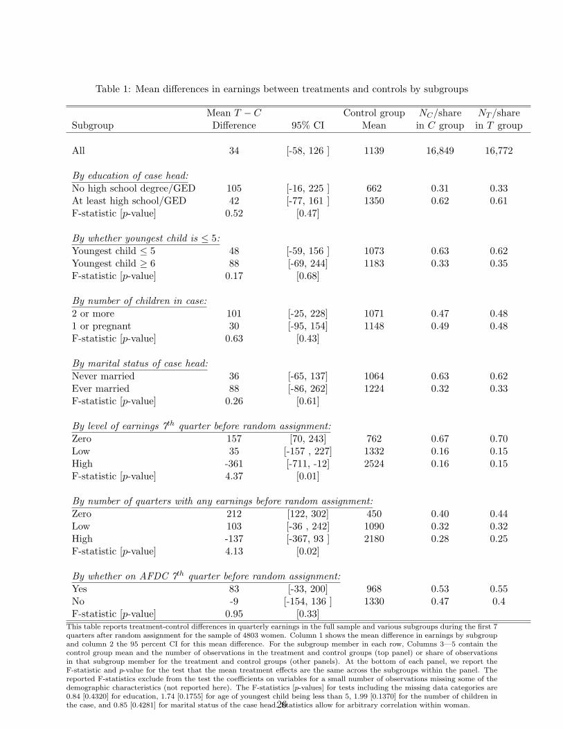
Table 1: Mean differences in earnings between treatments and controls by subgroups

Mean T − C Control group NC/share NT /shareSubgroup Difference 95% CI Mean in C group in T group

All 34 [-58, 126 ] 1139 16,849 16,772

By education of case head:No high school degree/GED 105 [-16, 225 ] 662 0.31 0.33At least high school/GED 42 [-77, 161 ] 1350 0.62 0.61F-statistic [p-value] 0.52 [0.47]

By whether youngest child is ≤ 5:Youngest child ≤ 5 48 [-59, 156 ] 1073 0.63 0.62Youngest child ≥ 6 88 [-69, 244] 1183 0.33 0.35F-statistic [p-value] 0.17 [0.68]

By number of children in case:2 or more 101 [-25, 228] 1071 0.47 0.481 or pregnant 30 [-95, 154] 1148 0.49 0.48F-statistic [p-value] 0.63 [0.43]

By marital status of case head:Never married 36 [-65, 137] 1064 0.63 0.62Ever married 88 [-86, 262] 1224 0.32 0.33F-statistic [p-value] 0.26 [0.61]

By level of earnings 7th quarter before random assignment:Zero 157 [70, 243] 762 0.67 0.70Low 35 [-157 , 227] 1332 0.16 0.15High -361 [-711, -12] 2524 0.16 0.15F-statistic [p-value] 4.37 [0.01]

By number of quarters with any earnings before random assignment:Zero 212 [122, 302] 450 0.40 0.44Low 103 [-36 , 242] 1090 0.32 0.32High -137 [-367, 93 ] 2180 0.28 0.25F-statistic [p-value] 4.13 [0.02]

By whether on AFDC 7th quarter before random assignment:Yes 83 [-33, 200] 968 0.53 0.55No -9 [-154, 136 ] 1330 0.47 0.4F-statistic [p-value] 0.95 [0.33]

This table reports treatment-control differences in quarterly earnings in the full sample and various subgroups during the first 7quarters after random assignment for the sample of 4803 women. Column 1 shows the mean difference in earnings by subgroupand column 2 the 95 percent CI for this mean difference. For the subgroup member in each row, Columns 3—5 contain thecontrol group mean and the number of observations in the treatment and control groups (top panel) or share of observationsin that subgroup member for the treatment and control groups (other panels). At the bottom of each panel, we report theF-statistic and p-value for the test that the mean treatment effects are the same across the subgroups within the panel. Thereported F-statistics exclude from the test the coefficients on variables for a small number of observations missing some of thedemographic characteristics (not reported here). The F-statistics [p-values] for tests including the missing data categories are0.84 [0.4320] for education, 1.74 [0.1755] for age of youngest child being less than 5, 1.99 [0.1370] for the number of children inthe case, and 0.85 [0.4281] for marital status of the case head. Statistics allow for arbitrary correlation within woman.26

Table 2: Permutation tests of equality of actual and simulated treatment group distributions,time-varying mean treatment effects by subgroup with participation adjustment

Unadj. Bonferroni adjusted# of Minimum # reject # reject Minimum

Subgroup Tests p-val at 10% at 5% p-valFull sample 7 <0.0003∗∗∗ 5 4 <0.0023∗∗∗

Education 21 0.0007∗∗∗ 3 1 0.0140∗∗

Age of youngest child 21 <0.0003∗∗∗ 2 2 <0.0070∗∗∗

Marital status 21 0.0003∗∗∗ 4 2 0.0070∗∗∗

Earnings level 7th Q pre-random assignment 21 0.0017∗∗∗ 2 1 0.0350∗∗

# pre-random assignment Q with earnings 21 0.0007∗∗∗ 1 1 0.0140∗∗

Welfare receipt 7th Q pre-random assignment 14 <0.0003∗∗∗ 3 3 <0.0047∗∗∗

Education subgroups interacted with:Age of youngest child 49 0.0020∗∗∗ 1 0 0.0980∗

Marital status 35 <0.0003∗∗∗ 3 3 <0.0117∗∗

Earnings level 7th Q pre-random assignment 63 0.0003∗∗∗ 1 1 0.0210∗∗

# pre-random assignment Q with earnings 63 0.0050∗∗∗ 0 0 0.3150Welfare receipt 7th Q pre-random assignment 42 0.0033∗∗∗ 0 0 0.1400Age of youngest child subgroup interacted with:Marital status 35 0.0027∗∗∗ 1 0 0.0933∗

Earnings level 7th Q pre-random assignment 63 0.0033∗∗∗ 0 0 0.2100# pre-random assignment Q with earnings 49 0.0010∗∗∗ 1 1 0.0490∗∗

Welfare receipt 7th Q pre-random assignment 42 0.0013∗∗∗ 1 0 0.0560∗

Marital status subgroup interacted with:Earnings level 7th Q pre-random assignment 63 0.0003∗∗∗ 1 1 0.0210∗∗

# pre-random assignment Q with earnings 63 0.0050∗∗∗ 0 0 0.3150Welfare receipt 7th Q pre-random assignment 42 <0.0003∗∗∗ 1 1 <0.0140∗∗

Earnings level 7th Q pre-random assignment subgroup interacted with:# pre-random assignment Q with earnings 49 0.0003∗∗∗ 0 0 0.1633Welfare receipt 7th Q pre-random assignment 42 <0.0003∗∗∗ 1 1 <0.0140∗∗

# of quarters any earnings pre-random assignment subgroup interacted with:Welfare receipt 7th Q pre-random assignment 42 0.0060∗∗∗ 0 0 0.2520

Notes: Table reports the result of tests of the nulls that simulated and actual CDFs are equal for those with positiveearnings within each subgroup and quarter for different set of subgroups. p-values adjusted using the Bonferroniadjustment, and represent the upper bound of the p-value. Thus the adjusted p-values for the full sample subgroupwhere seven tests are carried out (1 for each quarter) are the unadjusted p-values times 7. Test results reported incolumns 2–5. are the results of permutation tests of the KS statistic, following Praestgaard (1995). Each familyof tests for a number of mutually exclusive subgroups tests the null that the CDF for earnings for workers in thetreatment group is equal to the distribution obtained from adding time varying conditional mean earnings for thoseworking in the control group to the control group values, within each period and subgroup. The first column reportsthe number of tests for each family of subgroups. The second column reports the smallest unadjusted p-value for thefamily of tests. The third and fourth columns report the number of tests where the Bonferroni adjusted p-value forthe permutation KS test rejects at the 10% level and 5% level, respectively. The fifth column reports the smallest ofthe Bonferroni adjusted p-values for this family of tests. The values in column 5 have ∗∗∗ if the smallest unadjustedp-value allows rejection at the 1 percent level, ∗∗ if the smallest adjusted p-value allows rejection at the 5 percentlevel, and ∗ if the smallest adjusted p-value allows rejection at the 10 percent level. The values in column 5 have∗∗∗ if the smallest adjusted p-value allows rejection at the 1 percent level, ∗∗ if the smallest adjusted p-value allowsrejection at the 5 percent level, and ∗ if the smallest adjusted p-value allows rejection at the 10 percent level. Formore details, see text.

27

Figure 1: Conditional QTE, using education and earnings prior to random assignment to definesubgroups

(a) Education: Subgroup QTE

−800

−400

0

400

800

10 20 30 40 50 60 70 80 90Percentile index

HS grad.HS DO

(b) Earnings 7Q pre-random assignment: Sub-group QTE

−800

−400

0

400

800

10 20 30 40 50 60 70 80 90Percentile index

High LowZero

Notes: Figures for subgroups defined by education (left) and subgroups defined by earnings the 7thquarter before random assignment (right). Graphs show conditional QTE within each educationsubgroup (left graph) or earnings during the 7th quarter before random assignment (right graph).

28

Figure 2: Actual and simulated QTE, subgroups based on education (top graphs): and earningsand welfare use before random assignment (bottom graphs)

(a) Education: Time invariant

−800

−400

0

400

800

10 20 30 40 50 60 70 80 90Percentile index

Actual Simulated

(b) Education: Time varying

−800

−400

0

400

800

10 20 30 40 50 60 70 80 90Percentile index

Actual Simulated

(c) Earnings 7Q pre-random assignment: Timevarying

−800

−400

0

400

800

10 20 30 40 50 60 70 80 90Percentile index

Actual Simulated

(d) Any welfare 7Q pre-random assignment:Time varying

−800

−400

0

400

800

10 20 30 40 50 60 70 80 90Percentile index

Actual Simulated

Notes: In each figure, the solid line plots the actual QTE, and the dashed line plots the simulatedQTE. In all figures, we allow for either time invariant or time varying program effects on meanearnings within subgroup. -In the top graphs, subgroups are based on education. In the bottomgraphs, subgroups are based on earnings 7 quarters before random assignment (left) or welfarehistory before random assignment (right). In the left top figure, simulated earnings are calculatedunder the constraint that subgroup-specific treatment effects are constant across quarter. In theright top and bottom two figures, we allow the subgroup-specific treatment effects to vary acrossquarters.

29

Figure 3: Actual and simulated QTE with participation adjustment and time varying means,various subgroups

(a) Education

−800

−400

0

400

800

10 20 30 40 50 60 70 80 90Percentile index

Actual Simulated

(b) Earnings 7Q pre-random assignment

−800

−400

0

400

800

10 20 30 40 50 60 70 80 90Percentile index

Actual Simulated

(c) # pre-random assignment Q with earnings

−800

−400

0

400

800

10 20 30 40 50 60 70 80 90Percentile index

Actual Simulated

(d) Any welfare 7Q pre-random assignment

−800

−400

0

400

800

10 20 30 40 50 60 70 80 90Percentile index

Actual Simulated

Notes: In each figure, the solid line plots the actual QTE and the dashed line plots the simulatedQTE. In all figures, we allow for time-varying program effects on conditional mean earnings withinsubgroup. Data for simulated QTE constrained to have the share of non-participants equal andthe mean treatment-control difference in earnings the same. In the top left graph, subgroups arebased on education. In the top right graph, subgroups are based on the level of earnings 7 quarterspre-random assignment. In the bottom left graph, subgroups are based on the number of quarterspre-random assignment with positive earnings. In the bottom right graph, subgroups are based onwelfare history pre-random assignment.

30