Embed Size (px)
Citation preview
Journal of International Economics 68 (2006) 267–295
www.elsevier.com/locate/econbase
Can the standard international business cycle model
explain the relation between trade and comovement?
M. Ayhan Kose a,*, Kei-Mu Yi b
a International Monetary Fund, 700 19th St., N.W., Washington, DC 20431, United Statesb Research Department, Federal Reserve Bank of Philadelphia, 10 Independence Mall, Philadelphia,
PA 19106, United States
Received 11 December 2002; received in revised form 25 April 2005; accepted 5 July 2005
Abstract
Recent empirical research finds that pairs of countries with stronger trade linkages tend to have
more highly correlated business cycles. We assess whether the standard international business cycle
framework can replicate this intuitive result. We employ a three-country model with transportation
costs. We simulate the effects of increased goods market integration under two asset market
structures, complete markets and international financial autarky. Our main finding is that under both
asset market structures the model can generate stronger correlations for pairs of countries that trade
more, but the increased correlation falls far short of the empirical findings. Even when we control for
the fact that most country-pairs are small with respect to the rest-of-the-world, the model continues to
fall short. We also conduct additional simulations that allow for increased trade with the third country
or increased TFP shock comovement to affect the country-pair’s business cycle comovement. These
simulations are helpful in highlighting channels that could narrow the gap between the empirical
findings and the predictions of the model.
D 2005 Elsevier B.V. All rights reserved.
Keywords: International trade; International business cycle comovement
JEL classification: F4
0022-1996/$ -
doi:10.1016/j.
* Correspon
E-mail add
see front matter D 2005 Elsevier B.V. All rights reserved.
jinteco.2005.07.002
ding author.
resses: [email protected] (M.A. Kose), [email protected] (K.-M. Yi).

M.A. Kose, K.-M. Yi / Journal of International Economics 68 (2006) 267–295268
1. Introduction
Do countries that trade more with each other have more closely synchronized
business cycles? Yes, according to the conventional wisdom. Increased trade simply
increases the magnitude of the transmission of shocks between two countries. Although
this wisdom has circulated widely for a long time, it was not until recently that empirical
research was undertaken to assess its validity. Running cross-country or cross-region
regressions, first Frankel and Rose (FR, 1998), and then, Clark and van Wincoop
(2001), Otto et al. (2001), Calderon et al. (2002), Baxter and Kouparitsas (2004), and
others have all found that, among industrialized countries, pairs of countries that trade
more with each other exhibit a higher degree of business cycle comovement.1 Using
updated data, we re-estimate the FR regressions, and find that a doubling of the median
(across all country-pairs) bilateral trade intensity is associated with an increase in the
country-pair’s GDP correlation of about 0.06. These empirical results are all statistically
significant, and they suggest that increased international trade may lead to a significant
increase in output comovement.
While the results are in keeping with the conventional wisdom, it is important to
interpret them from the lens of a formal theoretical framework. The international real
business cycle (RBC) framework is a natural setting for this purpose because it is one of
the workhorse frameworks in international macroeconomics, and because it embodies the
demand and supply side spillover channels that many economists have in mind when they
think about the effect of increased trade on comovement. For example, in the workhorse
Backus et al. (1994) model, final goods are produced by combining domestic and foreign
intermediate goods. Consequently, an increase in final demand leads to an increase in
demand for foreign intermediates.
The impact of international trade on the degree of business cycle comovement has yet
to be studied carefully with this framework, as FR note: bthe large international real
business cycle literature, which does endogenize [output correlations]. . . does not focus
on the effects of changing economic integration on. . . business cycle correlationsQ.2 Thegoal of this paper is to focus on these effects by assessing whether the international RBC
framework is capable of replicating the strong empirical findings discussed above. We
develop, calibrate, and simulate an international business cycle model designed to
address whether increased trade is associated with increased GDP comovement. Our
model extends the BKK model in three ways. First, recent research by Heathcote and
Perri (2002) shows that an international RBC model with no international financial asset
markets (international financial autarky) generates a closer fit to several key business
cycle moments than does the model in a complete market setting or a one-bond setting.
Based on this work, in our model we study settings with international financial autarky,
1 Anderson et al. (1999) also find that there is a positive association between trade volume and the degree of
business cycle synchronization. Canova and Dellas (1993) and Imbs (2004) find that international trade plays a
relatively moderate role in transmitting business cycles across countries.2 FR, pp. 1015–1016. While several papers (that we cite in footnote 12) have looked at the relationship between
trade and business cycle comovement, their focus was not on explaining the recent cross-sectional empirical
research.
M.A. Kose, K.-M. Yi / Journal of International Economics 68 (2006) 267–295 269
as well as complete markets. Second, in the above empirical work, the authors recognize
the endogeneity of trade and instrument for it. In our framework, we introduce
transportation costs as a way of introducing variation in trade. Different levels of
transportation costs will translate into different levels of trade with consequent effects on
GDP comovement.
The typical international business cycle model is cast in a two-country setting. Indeed,
in a previous paper (Kose and Yi, 2001), we partially addressed the issue of this paper
using a two-country model. We argued that the model was able to explain about one-third
to one-half of the FR findings; our conclusion was that the model had failed to replicate
these findings. However, it turns out that this setting is inappropriate for capturing the
empirical link between trade and business cycle comovement. In particular, in a two-
country setting, by definition, the (single) pair of countries constitutes the entire world, and
one country is always at least one-half of the world economy. This would appear to grossly
exaggerate the impact of a typical country on another. In reality, a typical pair of countries
is small compared to the rest-of-the-world. Also, a typical country-pair trades much less
with each other than it does with the rest-of-the world. Moreover, Anderson and van
Wincoop (2003) carefully show theoretically and empirically that bilateral trading
relationships depend on each country’s trade barrier with the rest-of-the-world.
Consequently, a more appropriate framework is one that captures the facts that pairs of
countries tend to be small relative to the rest-of-the-world, pairs of countries trade much
less with each other than they do with the rest-of-the-world, and bilateral trade patterns
depend on trading relationships with the rest-of-the-world. These forces can only be
captured in a setting with at least three countries. This is our third, and most important,
modification of the BKK model.
Our three-country model is calibrated to be as close to our updated FR regressions
as possible. In particular, two of our countries are calibrated to two countries from the
FR sample (the country-pair), and the third country is calibrated to the other 19
countries, taken together (the rest-of-the-world). We choose four country-pairs, all of
which are close to the median bilateral trade intensity and GDP correlation. We solve
and simulate our model under a variety of transport costs between the two small
countries. Following the empirical research, we compute the change in GDP correlation
per unit change in the log of bilateral trade intensity. We find that under either set of
market structures, the model can match the empirical findings qualitatively, but it falls
far short quantitatively. In our baseline experiment, the model explains at most 1/10th
of the responsiveness of GDP comovement to trade intensity found in our updated FR
regressions.
A key reason for the model’s weak performance is that the trade intensity for each of
our benchmark country-pairs is small to begin with. A typical country does not trade much
with any other country: the median trade intensity in our sample is 0.0023, or
approximately 1/4 of 1% of GDP. For trade intensities close to the median, a doubling
or tripling is not a large increase in level terms. Moreover, we perform simulations
indicating that what matters for the model is the change in trade intensity levels, not logs.
Consequently, we re-estimate the FR regressions using trade intensity levels. We also
compute the responsiveness of GDP comovement to trade intensity levels implied by our
model and compare it to the new coefficient estimates. Now the model performs better. For

M.A. Kose, K.-M. Yi / Journal of International Economics 68 (2006) 267–295270
the best benchmark country-pair, the model implies that a one percentage point increase in
trade intensity (roughly 1% of GDP) would increase their GDP correlation by about 0.036,
which is more than 1/4 of the empirical findings. Nevertheless, for the other country-pairs
the model continues to fall short by more than an order of magnitude.
While the model performs even better when we employ a lower Armington elasticity of
substitution, there is still a sufficient gap between the model and the empirical findings that
it is suggestive of a trade–comovement puzzle. This puzzle would be distinct from the
puzzles that Obstfeld and Rogoff (2001) document; in particular, it is different from the
consumption correlation puzzle. The consumption correlation puzzle is about the inability
of the standard international business cycle models to generate the ranking of cross-
country output and consumption correlations in the data. Our trade–comovement puzzle is
about the inability of these models to generate a strong change in output correlations from
changes in bilateral trade intensity. In other words, the consumption correlation puzzle is
about the levels and ranking of output and consumption correlations, while the trade–
comovement puzzle is about a slope.
We conduct two further experiments that might help explain the gap between the model
and the empirical findings. In one experiment, we vary all transport costs, not just those
between the country-pair, but we attribute all of the correlation changes to changes in the
country-pair’s bilateral trade. This experiment yields a slope that is closer to, and in some
cases, exceeds, the empirically estimated slopes. We also find that the empirical
association between trade and total factor productivity (TFP) comovement is almost as
strong as the association between trade and GDP comovement. We conduct an experiment
in which as we vary transport costs and trade, the correlation of TFP shocks changes in a
way that is consistent with our regressions. Now there are two channels affecting GDP
correlation, the pure trade channel, and an indirect channel operating through TFP
comovement. Not surprisingly, the model does a much better job in this experiment. Both
of our experiments provide guidance for future empirical and modeling work on resolving
this puzzle.
In Section 2, we update the Frankel–Rose regressions to study the empirical
relationship between trade and business cycle comovement. Next, we describe our
three-country model and its parameterization. Our quantitative assessment of the model is
conducted in Section 4. Section 5 concludes.
2. Empirical link between trade and comovement
We update the Frankel–Rose (FR) regressions, which employed quarterly data running
from 1959 to 1993. Our sample covers the same 21 OECD countries as in FR, but our data
are annual, and cover the period 1970–2000. We employ one of the FR measures of
bilateral trade intensity, the sum of each country’s imports from the other divided by the
sum of their GDPs, averaged over the entire period. The median bilateral trade intensity
(hereafter btrade intensityQ) over all countries and all years is 0.0023, and the standard
deviation of the trade shares is 0.0098. We employ two of the FR measures of business
cycle comovement, Hodrick–Prescott (HP) filtered and (log) first-differenced correlations
of real GDP between the two countries. Summary statistics of the trade and comovement

Table 1
Empirical link between trade and business cycle comovement
(a) Descriptive statistics
Bilateral trade
intensity
HP-filtered
correlation GDP
Log first-differenced
GDP correlation
Median 0.0023 0.42 0.34
Minimum 0.0002 �0.57 �0.32Maximum 0.0727 0.93 0.83
Standard deviation 0.0098 0.35 0.22
(b) Estimation results (updated Frankel–Rose regressions)
Coefficient on trade intensity
Logs Levels
HP-filtered GDP 0.091 (0.022) 12.557 (3.760)
Log first-differenced GDP 0.078 (0.014) 11.262 (2.859)
(c) Trade and comovement properties of benchmark country-pairs
Country-pair Bilateral trade
intensity
HP-filtered
GDP correlation
Log first-differenced
GDP correlation
Belgium–U.S, 0.0019 0.403 0.359
Australia–Belgium 0.0015 0.442 0.363
Finland–Portugal 0.0017 0.452 0.377
France–U.S. 0.0040 0.434 0.363
Annual GDP and trade data for 21 OECD countries, 1970–2000, are from IMF’s International Financial Statistics
and Direction of Trade Statistics. Bilateral trade intensity is sum of imports divided by sum of GDPs, averaged
over 1970–2000. GMM estimation of GDP correlation on a constant and log or level of trade intensity. Standard
errors in parentheses. Instrumental variables for trade intensity are log of distance, adjacency dummy, and
common language, and are obtained from Andrew Rose’s web site: http://faculty.haas.berkeley.edu/arose/
RecRes.htm.
M.A. Kose, K.-M. Yi / Journal of International Economics 68 (2006) 267–295 271
data are presented in Table 1a, and the data for HP-filtered GDP are illustrated in Fig. 1.
While the data look cloudy, there is also a fairly clear positive slope.3
We estimate two (cross-section) regressions. In the first, we follow FR by running
instrumental variables (IV) estimation on the log of trade intensity:
Corrij ¼ b0 þ b1ln Tradeij� �
þ eij ð1Þ
where i and j denote the two countries. In the second, we run the regression on the levels
of Tradeij:
Corrij ¼ b0 þ b1Tradeij þ eij: ð2Þ
As mentioned in the introduction, the regressions using the log of trade intensity imply that
an increase in a country-pair’s trade intensity from 0.002 to 0.004 is associated with the
same change in its GDP correlation as an increase in its trade intensity from 0.02 to 0.04.
This would appear to be counterfactual, which motivates our second regression, in which
3 Baxter and Kouparitsas (2004) produce a similar figure using data from developed and developing countries.

FinPortAusBelg BelgUS
FR-US
-0.8
-0.6
-0.4
-0.2
0
0.2
0.4
0.6
0.8
1
1.2
-9 -8 -7 -6 -5 -4 -3 -2 -1 0
(log) Bilateral Trade Intensity
HP Filtered GDPCorrelation
Fig. 1. GDP correlation and trade intensity.
M.A. Kose, K.-M. Yi / Journal of International Economics 68 (2006) 267–295272
trade intensity is measured in level terms. We employ a GMM instrumental variable
estimator that corrects for heteroskedasticity in the error terms. Our instruments for Tradeijare the same as in FR: a dummy variable for whether the two countries are adjacent, a
dummy variable for whether the two countries share a common language, and the log of
distance. The coefficients on trade intensity are listed in Table 1b.
Our estimates are consistent with those in the empirical literature. In the logs
regression, the slope coefficient estimate implies that a country-pair with twice the trade
intensity as another country-pair will have a 0.063 (HP-filtered GDP) or 0.054 (log first-
differenced GDP) higher GDP correlation, all else equal.4 FR’s estimates with HP-filtered
GDP imply that a doubling of trade intensity is associated with a 0.033 higher GDP
correlation. The slope coefficient from our levels regression implies that a doubling of the
median trade intensity, i.e., an increase of 0.0023, is associated with an increase in GDP
correlation of about 0.029 (HP-filtered GDP) or 0.026 (log first-differenced GDP). Note
that these numbers are about half as large as what is implied from the logs regression. We
also examined two other measures of trade intensity, the sum of each country’s imports
from each other divided by the sum of their total imports, and bilateral imports divided by
total imports of the smaller of the two countries. The results are very similar to those
obtained with our benchmark measure of trade intensity.5
4 Running the logs regression with OLS yields a coefficient of 0.05, which is about half of the GMM
coefficient. Consequently, controlling for the endogeneity of trade generates a stronger relationship than would be
suggested by Fig. 1.5 The motivation for the second measure comes from the idea that a high GDP correlation seems to arise from a
large bilateral trade share (of total trade) by the smaller of the two countries. For the first measure, and for the HP-
filtered data (the first-differenced results are very similar) a doubling of the median trade intensity is associated
with an increase in GDP correlation of 0.08 (logs) and 0.035 (levels). For the second measure, a doubling of the
median trade intensity is associated with an increase in GDP correlation of 0.08 (logs) and 0.051 (levels).
M.A. Kose, K.-M. Yi / Journal of International Economics 68 (2006) 267–295 273
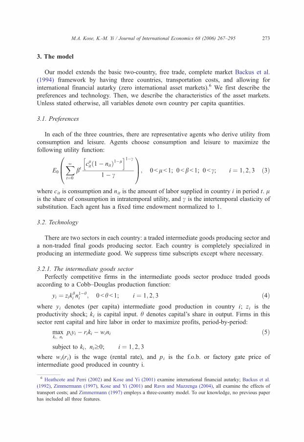
3. The model
Our model extends the basic two-country, free trade, complete market Backus et al.
(1994) framework by having three countries, transportation costs, and allowing for
international financial autarky (zero international asset markets).6 We first describe the
preferences and technology. Then, we describe the characteristics of the asset markets.
Unless stated otherwise, all variables denote own country per capita quantities.
3.1. Preferences
In each of the three countries, there are representative agents who derive utility from
consumption and leisure. Agents choose consumption and leisure to maximize the
following utility function:
E0
Xlt¼0
btclit 1� nitð Þ1�l
h i1�c
1� c
0B@
1CA; 0blb 1; 0bbb 1; 0b c; i ¼ 1; 2; 3 ð3Þ
where cit is consumption and nit is the amount of labor supplied in country i in period t. lis the share of consumption in intratemporal utility, and c is the intertemporal elasticity of
substitution. Each agent has a fixed time endowment normalized to 1.
3.2. Technology
There are two sectors in each country: a traded intermediate goods producing sector and
a non-traded final goods producing sector. Each country is completely specialized in
producing an intermediate good. We suppress time subscripts except where necessary.
3.2.1. The intermediate goods sector
Perfectly competitive firms in the intermediate goods sector produce traded goods
according to a Cobb–Douglas production function:
yi ¼ zikhi n
1�hi ; 0bhb 1; i ¼ 1; 2; 3 ð4Þ
where yi denotes (per capita) intermediate good production in country i; zi is the
productivity shock; ki is capital input. h denotes capital’s share in output. Firms in this
sector rent capital and hire labor in order to maximize profits, period-by-period:
maxki; ni
piyi � riki � wini ð5Þ
subject to ki; niz0; i ¼ 1; 2; 3
where wi(ri) is the wage (rental rate), and pi is the f.o.b. or factory gate price of
intermediate good produced in country i.
6 Heathcote and Perri (2002) and Kose and Yi (2001) examine international financial autarky; Backus et al.
(1992), Zimmermann (1997), Kose and Yi (2001) and Ravn and Mazzenga (2004), all examine the effects of
transport costs; and Zimmermann (1997) employs a three-country model. To our knowledge, no previous paper
has included all three features.

M.A. Kose, K.-M. Yi / Journal of International Economics 68 (2006) 267–295274
The market clearing condition in each period for the intermediate goods producing
firms in country i is:
X3j¼1
pjyij ¼ piyi ð6Þ
where pi is the number of households in country i, and determines country size. yij denotes
the quantity of intermediates produced in country i and shipped to each agent in country j.
The total number of households in the world is normalized to 1:
X3i¼1
pi ¼ 1: ð7Þ
3.2.2. Transportation costs
When the intermediate goods are exported to the other country, they are subject to
transportation costs. We think of these costs as a stand-in for tariffs and other non-tariff
barriers, as well as transport costs. Following Backus et al. (1992) and Ravn and Mazzenga
(1999), we model the costs as quadratic iceberg costs. This formulation of transport costs
generalizes the standard Samuelson linear iceberg specification and takes into account that
transportation costs become higher as the amount of traded goods gets larger.7 Specifically,
if country i exports yij units to country j, gij( yij)2 units are lost in transit, where gij is the
transport cost parameter for country i’s exports to country j. That is, only:
1� gijyij� �
yijumij ð8Þunits are imported by country j. We think of gijyij as the iceberg transportation cost; it is the
fraction of the exported goods that are lost in transit. In our simulations,we evaluate the transport
costs at the steady-state values of yij. Below, we discuss our transport technology further.
3.2.3. The final goods sector
Each country’s output of intermediates is used as an input into final goods production.
Final goods firms in each country produce their goods by combining domestic and foreign
intermediates via an Armington aggregator. To be more specific, the final goods
production function in country j is given by:
F y1j; y2j; y3j� �
¼X3i¼1
xij 1� gijyij� �
yij� �1�a
" #1= 1�að Þ
ð9Þ
¼X3i¼1
xijm1�aij
" #1= 1�að Þ
ð10Þ
x1j;x2j;x3j[0; a[0; j ¼ 1; 2; 3
7 An additional reason for using quadratic costs is that our linearization solution procedure eliminates any
marginal impact of the usual linear or proportional costs. For transport costs to have "bite" in our framework, non-
linear costs are needed.

M.A. Kose, K.-M. Yi / Journal of International Economics 68 (2006) 267–295 275
where x1j denotes the Armington weight applied to the intermediate good produced by
country 1 and imported by country j (m1j). We assume that gii =0 and that gijyij =gjiyji. In
other words, there is no cost associated with intra-country trade, i.e., m22=y22, and iceberg
transport costs between two countries do not depend on the origin of the goods. 1/a is the
elasticity of substitution between the inputs.
Final goods producing firms in each country j maximize profits, period-by-period:
maxm1j;m2j;m3j
qjX3i¼1
xijm1�aij
" #1= 1�að Þ
� p1jm1j � p2jm2j � p3jm3j ð11Þ
where qj is the price of the final good produced by country j, and pij is the c.i.f. (cost,
insurance, and freight) price of country i’s good imported by country j. Note that pjj =pj.
The non-traded good in country 1 is the numeraire good; hence, q1=1.
As in Ravn and Mazzenga (1999), we can use the first-order conditions from (11) to
calculate the price of an imported good i relative to j’s own good:
pij
pj¼ xij
xjj
yjj
mij
� �a
: ð12Þ
Also, because BF/Byij =(BF/Bmij)(1�2gijyij), we know that:
pi ¼ 1� 2gijyij� �
pij: ð13Þ
Comparing (8) and (13), it is easy to see that the c.i.f. price multiplied by imports exceeds
the f.o.b. price multiplied by exports:
pijmij � piyij ¼ pij 1� gijyij� �
yij � piyij ¼ yij pij 1� gijyij� �
� pi� �
N0: ð14Þ
In other words, if we think of the transportation costs as arising from transportation
services provided to ship goods between countries, with the quadratic costs arising
because the transportation technology is decreasing returns to scale, then, in a perfect
competition setting, there are positive profits. That is, the firms providing the
transportation services pay the exporting firm the factory gate or f.o.b. price of the good,
and then receive the c.i.f. price from the final goods firm in the importing country. We
think of a single representative shipping firm that chooses yij to maximize the leftmost
expression of (14). We assume that households in the exporting country own this firm,
whose profits are distributed as dividends to the households.
Capital is accumulated in the standard way:
kjtþ1 ¼ 1� dð Þkjt þ xjt; j ¼ 1; 2; 3 ð15Þ
where xit is investment, and d is the rate of depreciation. Final goods are used for domestic
consumption and investment in each country:
cjt þ xjt ¼ F y1jt; y2jt; y3jt� �
; j ¼ 1; 2; 3: ð16Þ

M.A. Kose, K.-M. Yi / Journal of International Economics 68 (2006) 267–295276
3.3. Asset markets
We consider two asset market structures, (international) financial autarky and complete
markets. Under financial autarky, there is no asset trade; hence, trade is balanced period by
period. As mentioned above, Heathcote and Perri (2002) have shown that international
business cycle models with financial autarky yield a closer fit to some key business cycle
moments than the same models under complete markets. Also, financial autarky is the
natural other extreme relative to complete markets.8 The following budget constraint must
hold in each period:
qit cit þ xitð Þ � ritkit � witnit � Rit ¼ 0; 8t ¼ 0; N ;l; i ¼ 1; 2; 3 ð17Þ
where Rit is profits that the transportation firms distribute as dividends to the household
¼P2
j¼1 pijtmijt � pityijt� ��
. In addition to dividends, the household obtains income
from its labor and from the capital it owns. The household spends its income on
consumption and investment goods. The complete markets framework, i.e., complete
contingent claims or fully integrated international asset markets, is the usual benchmark.
We follow Heathcote and Perri (2002) in assuming there are complete contingent claims
denominated in units of one of the countries’ tradable (intermediate) good (say country 1).
Let st denote the particular state of the economy in period t, and let st denote the complete
history of events up until date t. Also, let Bi(st,st+1) denote the quantity of bonds
purchased by the household in country i after history st that pays one unit of country 1’s
tradable good if and only if state st+1 occurs; P(st,st+1) is the price of these bonds in units
of country 1’s tradable good. Then, we can write the budget constraint for country i in
period t as follows:
qi stð Þ ci stð Þ þ xi s
tð Þð Þ þ p1i stð ÞXstþ1
P st; stþ1ð ÞBi st; stþ1ð Þ
¼ ri stð Þki stð Þ þ wi s
tð Þni stð Þ þ p1i stð ÞBi s
t�1; st� �
þ Ri stð Þ: ð18Þ
Households maximize (3) subject to either (17) or (18).
3.4. Equilibrium
Definition 1. An equilibrium is a sequence of goods and factor prices and quantities such
that the first-order conditions to the firms’ and households’ maximization problems, as
well as market clearing conditions (6) and (16) are satisfied in every period.
3.5. Calibration and solution
Our goal is to quantitatively assess whether our three-country international RBC model
can generate the high responsiveness of GDP comovement to bilateral trade intensity
8 A third asset structure that is popular involves one-period risk-free bonds. However, recent research by
Heathcote and Perri (2002), Baxter and Crucini (1995), and others suggest that, when productivity shocks are
stationary, a bond economy typically implies results very similar to those of a complete markets economy.
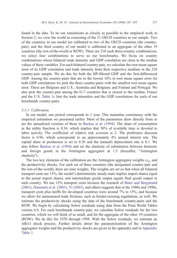
M.A. Kose, K.-M. Yi / Journal of International Economics 68 (2006) 267–295 277
found in the data. To tie our simulations as closely as possible to the empirical work in
Section 2, we view the world as consisting of the 21 OECD countries in our sample. Two
of the countries in our model are calibrated to two of the OECD countries (the country-
pair), and the third country of our model is calibrated to an aggregate of the other 19
countries (the rest-of-the-world or ROW). There are 210 such three-country combinations;
we select four combinations to serve as our benchmarks. We focus on country
combinations whose bilateral trade intensity and GDP correlation are close to the median
values of these variables. For each bilateral country-pair, we calculate the root mean square
error of its GDP correlation and trade intensity from their respective medians in the 210
country-pair sample. We do this for both the HP-filtered GDP and the first-differenced
GDP. Among the country-pairs that are in the lowest 10% in root mean square error for
both GDP correlations we pick the three country-pairs with the smallest root mean square
error. These are Belgium and U.S.; Australia and Belgium; and Finland and Portugal. We
also pick the country-pair among the G-7 countries that is closest to the median: France
and the U.S. Table 1c lists the trade intensities and the GDP correlations for each of our
benchmark country-pairs.
3.5.1. Calibration
In our model, one period corresponds to 1 year. This maintains consistency with the
empirical estimation we presented earlier. Most of the parameters draw directly from or
are the annualized versions of those in Backus et al. (1994). The share of consumption
in the utility function is 0.34, which implies that 30% of available time is devoted to
labor activity. The coefficient of relative risk aversion is 2. The preference discount
factor is 0.96, which corresponds to an approximately 4% annual interest rate. The
capital share in production is set to 0.36 and the (annual) depreciation rate is 0.1. We
also follow Backus et al. (1994) and set the elasticity of substitution between domestic
and foreign goods in the Armington aggregator at 1.5 (hereafter, bArmington
elasticityQ).The two key elements of the calibration are the Armington aggregator weights xij, and
the productivity shocks. For each set of three countries (the designated country-pair and
the rest-of-the-world), there are nine weights. The weights are set so that when all bilateral
transport costs are 15%, the model’s deterministic steady-state implies import shares equal
to the actual import shares, and intermediate goods output equals final goods output in
each country. We use 15% transport costs because the research of Baier and Bergstrand
(2001), Hummels et al. (2001), Yi (2003), and others suggests that in the 1980s and 1990s,
transport costs plus tariffs for developed countries were around 7% to 15%, and because
we allow for unmeasured trade frictions, such as border-crossing regulations, as well. We
estimate the productivity shocks using the data of the benchmark country-pairs and the
ROW. We begin by calculating Solow residuals using data from the Penn World Tables
version 6.0. For each benchmark country-pair, we calculate Solow residuals for the two
countries, which we will think of as small, and for the aggregate of the other 19 countries
(ROW). We do this for 1970 through 1998. With the Solow residuals, we estimate an
AR(1) shock process. Further details about the parameterization of the Armington
aggregator weights and the productivity shocks are given in the appendix and in Appendix
Table 1.
M.A. Kose, K.-M. Yi / Journal of International Economics 68 (2006) 267–295278
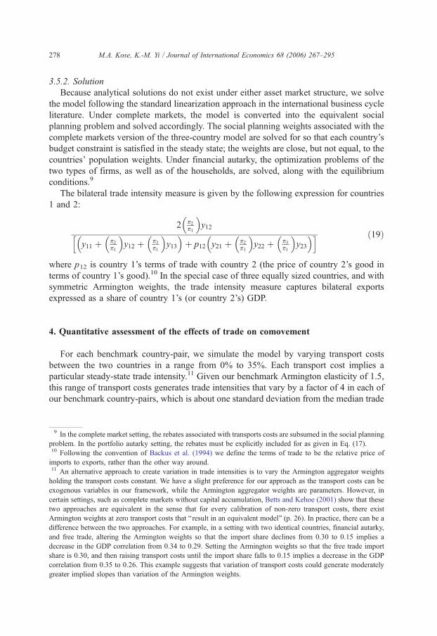
3.5.2. Solution
Because analytical solutions do not exist under either asset market structure, we solve
the model following the standard linearization approach in the international business cycle
literature. Under complete markets, the model is converted into the equivalent social
planning problem and solved accordingly. The social planning weights associated with the
complete markets version of the three-country model are solved for so that each country’s
budget constraint is satisfied in the steady state; the weights are close, but not equal, to the
countries’ population weights. Under financial autarky, the optimization problems of the
two types of firms, as well as of the households, are solved, along with the equilibrium
conditions.9
The bilateral trade intensity measure is given by the following expression for countries
1 and 2:
2 p2
p1
� y12
y11 þ p2
p1
� y12 þ p3
p1
� y13
� þ p12 y21 þ p2
p1
� y22 þ p3
p1
� y23
� h i ð19Þ
where p12 is country 1’s terms of trade with country 2 (the price of country 2’s good in
terms of country 1’s good).10 In the special case of three equally sized countries, and with
symmetric Armington weights, the trade intensity measure captures bilateral exports
expressed as a share of country 1’s (or country 2’s) GDP.
4. Quantitative assessment of the effects of trade on comovement
For each benchmark country-pair, we simulate the model by varying transport costs
between the two countries in a range from 0% to 35%. Each transport cost implies a
particular steady-state trade intensity.11 Given our benchmark Armington elasticity of 1.5,
this range of transport costs generates trade intensities that vary by a factor of 4 in each of
our benchmark country-pairs, which is about one standard deviation from the median trade
9 In the complete market setting, the rebates associated with transports costs are subsumed in the social planning
problem. In the portfolio autarky setting, the rebates must be explicitly included for as given in Eq. (17).10 Following the convention of Backus et al. (1994) we define the terms of trade to be the relative price of
imports to exports, rather than the other way around.11 An alternative approach to create variation in trade intensities is to vary the Armington aggregator weights
holding the transport costs constant. We have a slight preference for our approach as the transport costs can be
exogenous variables in our framework, while the Armington aggregator weights are parameters. However, in
certain settings, such as complete markets without capital accumulation, Betts and Kehoe (2001) show that these
two approaches are equivalent in the sense that for every calibration of non-zero transport costs, there exist
Armington weights at zero transport costs that bresult in an equivalent model Q (p. 26). In practice, there can be a
difference between the two approaches. For example, in a setting with two identical countries, financial autarky,
and free trade, altering the Armington weights so that the import share declines from 0.30 to 0.15 implies a
decrease in the GDP correlation from 0.34 to 0.29. Setting the Armington weights so that the free trade import
share is 0.30, and then raising transport costs until the import share falls to 0.15 implies a decrease in the GDP
correlation from 0.35 to 0.26. This example suggests that variation of transport costs could generate moderately
greater implied slopes than variation of the Armington weights.
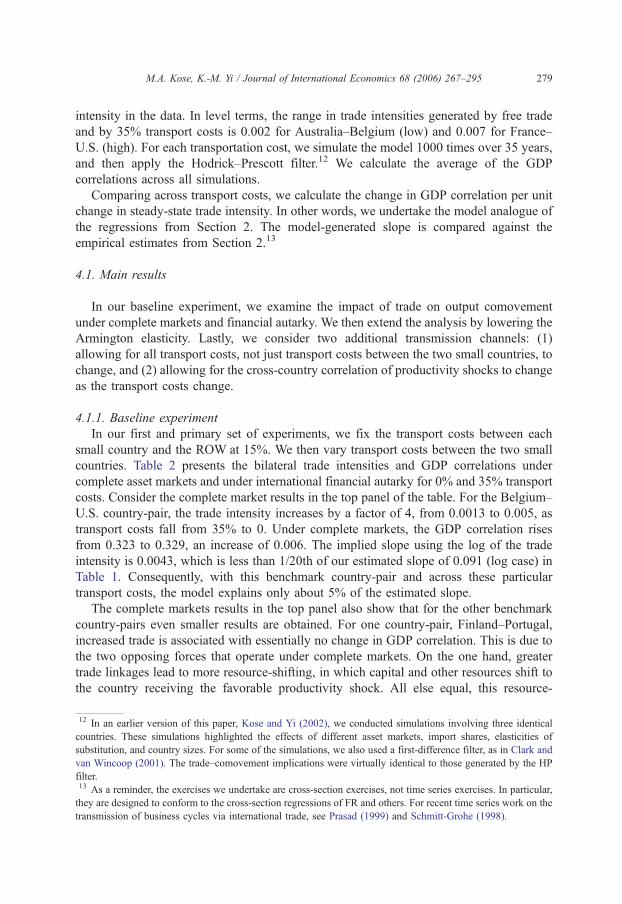
M.A. Kose, K.-M. Yi / Journal of International Economics 68 (2006) 267–295 279
intensity in the data. In level terms, the range in trade intensities generated by free trade
and by 35% transport costs is 0.002 for Australia–Belgium (low) and 0.007 for France–
U.S. (high). For each transportation cost, we simulate the model 1000 times over 35 years,
and then apply the Hodrick–Prescott filter.12 We calculate the average of the GDP
correlations across all simulations.
Comparing across transport costs, we calculate the change in GDP correlation per unit
change in steady-state trade intensity. In other words, we undertake the model analogue of
the regressions from Section 2. The model-generated slope is compared against the
empirical estimates from Section 2.13
4.1. Main results
In our baseline experiment, we examine the impact of trade on output comovement
under complete markets and financial autarky. We then extend the analysis by lowering the
Armington elasticity. Lastly, we consider two additional transmission channels: (1)
allowing for all transport costs, not just transport costs between the two small countries, to
change, and (2) allowing for the cross-country correlation of productivity shocks to change
as the transport costs change.
4.1.1. Baseline experiment
In our first and primary set of experiments, we fix the transport costs between each
small country and the ROW at 15%. We then vary transport costs between the two small
countries. Table 2 presents the bilateral trade intensities and GDP correlations under
complete asset markets and under international financial autarky for 0% and 35% transport
costs. Consider the complete market results in the top panel of the table. For the Belgium–
U.S. country-pair, the trade intensity increases by a factor of 4, from 0.0013 to 0.005, as
transport costs fall from 35% to 0. Under complete markets, the GDP correlation rises
from 0.323 to 0.329, an increase of 0.006. The implied slope using the log of the trade
intensity is 0.0043, which is less than 1/20th of our estimated slope of 0.091 (log case) in
Table 1. Consequently, with this benchmark country-pair and across these particular
transport costs, the model explains only about 5% of the estimated slope.
The complete markets results in the top panel also show that for the other benchmark
country-pairs even smaller results are obtained. For one country-pair, Finland–Portugal,
increased trade is associated with essentially no change in GDP correlation. This is due to
the two opposing forces that operate under complete markets. On the one hand, greater
trade linkages lead to more resource-shifting, in which capital and other resources shift to
the country receiving the favorable productivity shock. All else equal, this resource-
12 In an earlier version of this paper, Kose and Yi (2002), we conducted simulations involving three identical
countries. These simulations highlighted the effects of different asset markets, import shares, elasticities of
substitution, and country sizes. For some of the simulations, we also used a first-difference filter, as in Clark and
van Wincoop (2001). The trade–comovement implications were virtually identical to those generated by the HP
filter.13 As a reminder, the exercises we undertake are cross-section exercises, not time series exercises. In particular,
they are designed to conform to the cross-section regressions of FR and others. For recent time series work on the
transmission of business cycles via international trade, see Prasad (1999) and Schmitt-Grohe (1998).
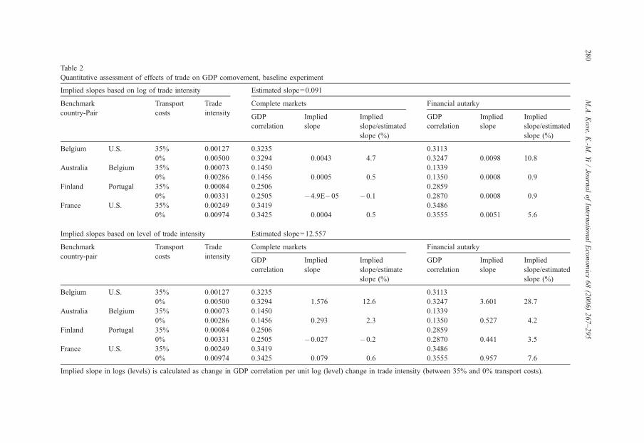
Table 2
Quantitative assessment of effects of trade on GDP comovement, baseline experiment
Implied slopes based on log of trade intensity Estimated slope=0.091
Benchmark
country-Pair
Transport
costs
Trade
intensity
Complete markets Financial autarky
GDP
correlation
Implied
slope
Implied
slope/estimated
slope (%)
GDP
correlation
Implied
slope
Implied
slope/estimated
slope (%)
Belgium U.S. 35% 0.00127 0.3235 0.3113
0% 0.00500 0.3294 0.0043 4.7 0.3247 0.0098 10.8
Australia Belgium 35% 0.00073 0.1450 0.1339
0% 0.00286 0.1456 0.0005 0.5 0.1350 0.0008 0.9
Finland Portugal 35% 0.00084 0.2506 0.2859
0% 0.00331 0.2505 �4.9E�05 �0.1 0.2870 0.0008 0.9
France U.S. 35% 0.00249 0.3419 0.3486
0% 0.00974 0.3425 0.0004 0.5 0.3555 0.0051 5.6
Implied slopes based on level of trade intensity Estimated slope=12.557
Benchmark
country-pair
Transport
costs
Trade
intensity
Complete markets Financial autarky
GDP
correlation
Implied
slope
Implied
slope/estimate
slope (%)
GDP
correlation
Implied
slope
Implied
slope/estimated
slope (%)
Belgium U.S. 35% 0.00127 0.3235 0.3113
0% 0.00500 0.3294 1.576 12.6 0.3247 3.601 28.7
Australia Belgium 35% 0.00073 0.1450 0.1339
0% 0.00286 0.1456 0.293 2.3 0.1350 0.527 4.2
Finland Portugal 35% 0.00084 0.2506 0.2859
0% 0.00331 0.2505 �0.027 �0.2 0.2870 0.441 3.5
France U.S. 35% 0.00249 0.3419 0.3486
0% 0.00974 0.3425 0.079 0.6 0.3555 0.957 7.6
Implied slope in logs (levels) is calculated as change in GDP correlation per unit log (level) change in trade intensity (between 35% and 0% transport costs).
M.A.Kose,
K.-M
.Yi/JournalofIntern
atio
nalEconomics
68(2006)267–295
280

M.A. Kose, K.-M. Yi / Journal of International Economics 68 (2006) 267–295 281
shifting force lowers business cycle comovement. Second, there is a trade-magnification
force: greater trade linkages lead to greater business cycle comovement because, loosely
speaking, of the usual supply and demand linkages mentioned previously. From the tables
we can infer that for the Finland–Portugal case, the two forces essentially cancel.14
Under financial autarky, the resource-shifting channel cannot operate, so the only
force at work is the trade-magnification force discussed above. Consequently, it is
natural to suppose that the model implied slopes would be closer to the estimated slope.
This is the case, as the right-hand side of the top panel of Table 2 shows. For the
Belgium–U.S. country-pair, for example, the GDP correlation rises from 0.3113 to
0.3247 as transport costs fall from 35% to 0, an increase of 0.0134. This increase is
more than double the increase in the complete market case. The implied slope, again
using the log of the trade intensity, is 0.0098, which is slightly more than 1/10 of our
estimated slope. The implied slopes for the other three country-pairs are all smaller than
the Belgium–U.S. slope. Relative to complete markets, the France–U.S. country-pair
showed the greatest increase; the implied slope is about 5.6% of our estimated slope,
which is 10 times higher than under complete markets. Hence, while financial autarky
does generate higher implied slopes than complete markets, the model is still off by an
order of magnitude or more.15
While the primary goal of this section is to provide a quantitative assessment of the
model, we believe it is useful at this point to provide a more thorough intuition on how the
trade-magnification force works, especially because this is the force that generates greater
comovement through increased trade.16 One country’s GDP is correlated with another’s to
the extent that its TFP, capital, and labor are correlated with the other country’s TFP,
capital, and labor. Capital is essentially fixed in the short run. The TFP processes are
exogenous and remain unchanged in our baseline experiment. Consequently, the increase
in GDP correlation due to lower transport costs must stem primarily from increases in the
two countries’ employment correlation.
The employment correlation, in turn, is driven by TFP shocks. Consider a pair of
countries. A positive TFP shock to one country, bOneQ, will raise output of One’s
intermediate good. Output of the intermediate good rises further because employment in
One rises. In addition, the relative price of One’s intermediate falls, i.e., One’s terms of
trade increase. This makes labor in the other country, bTwoQ, effectively more
productive, thus raising labor demand and employment in Two. It turns out that the
decrease in Two’s (increase in One’s) terms of trade is larger under free trade than under
transport costs. Hence, under free trade the employment and output response in Two is
14 Our finding that the model with complete asset markets can produce essentially no relationship between trade
intensity and business cycle comovement in the data is consistent with other research that has examined the
effects of transport costs on comovement including Backus et al. (1992), Zimmermann (1997), Kose and Yi
(2001, 2002), and Mazzenga and Ravn (2004). On the other hand, see Head (2002) for an international business
cycle model based on monopolistic competition. In this model, under complete markets, lower transport costs
leads to higher output comovement.15 For both complete markets and financial autarky, we calculated the model’s implied slope when transport
costs fall from 35% to 20%, from 20% to 10% and from 10% to 0%. The results are essentially the same. For
example, for Belgium–U.S. under financial autarky, the slopes are 0.005, 0.014, and 0.023, respectively.16 We thank one of the referees for suggesting much of the following intuition.
Output-Country 1
-0.2
0
0.2
0.4
0.6
0.8
1
1.2
0 5 10 15 20 25 30 35
Years
% D
evia
tion
fro
m S
tead
y S
tate
Free Trade
35% Transport Cost
Terms of Trade-Country 2
-4
-3
-2
-1
0
1
0 5 10 15 20 25 30 35
Years
% D
evia
tion
fro
m S
tead
y St
ate
Free Trade
35% Transport Cost
Output-Country 2
-0.05
0
0.05
0.1
0.15
0.2
0.25
0 5 10 15 20 25 30 35
Years
% D
evia
tion
fro
m S
tead
y St
ate
Free Trade
35% Transport Cost
a.
b.
c.
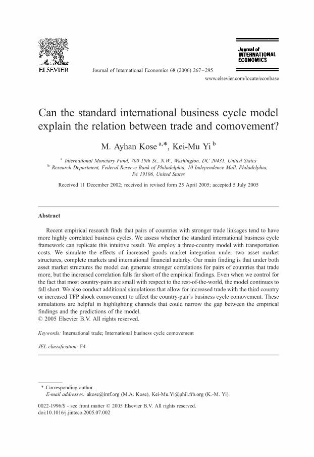
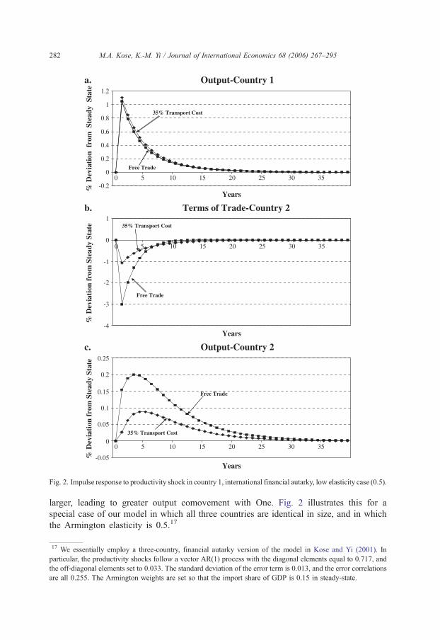
Fig. 2. Impulse response to productivity shock in country 1, international financial autarky, low elasticity case (0.5).
M.A. Kose, K.-M. Yi / Journal of International Economics 68 (2006) 267–295282
larger, leading to greater output comovement with One. Fig. 2 illustrates this for a
special case of our model in which all three countries are identical in size, and in which
the Armington elasticity is 0.5.17
17 We essentially employ a three-country, financial autarky version of the model in Kose and Yi (2001). In
particular, the productivity shocks follow a vector AR(1) process with the diagonal elements equal to 0.717, and
the off-diagonal elements set to 0.033. The standard deviation of the error term is 0.013, and the error correlations
are all 0.255. The Armington weights are set so that the import share of GDP is 0.15 in steady-state.

M.A. Kose, K.-M. Yi / Journal of International Economics 68 (2006) 267–295 283
The last part of the intuition addresses why Two’s terms of trade falls by more
under free trade than under transport costs. There are two channels operating. The
first channel begins with the idea that world demand for One’s good is the sum of
One’s demand and Two’s demand. One’s demand is less responsive to changes in
prices (steeper demand curve) because any price changes have both a substitution
effect and an income effect. A positive TFP shock in One leads to a decline in the
price of its good. Demand rises because of substitution effects, but this increase is
partially offset by the adverse income effect owing to the worsened terms of trade.
Two’s demand for One’s good, on the other hand, is driven mainly by the substitution
effect. This means Two’s demand curve is flatter. As the world moves to free trade,
Two’s share of world demand for One’s good increases; this means the overall world
demand curve becomes flatter, which would lead to a smaller fall in Two’s terms of
trade.
The second channel works in the opposite direction. As the world moves towards
free trade, the importance of the income effect for One’s response to its own
productivity shocks rises. This is because the income effect is realized to the extent the
country purchases imported goods. One’s demand curve becomes steeper; this
contributes to a steeper world demand curve, which, all else equal, would lead to a
steeper fall in Two’s terms of trade (in response to a positive TFP shock in One). Our
interpretation of the second panel of Fig. 2 is that this second channel dominates the
first channel. Summarizing, then, due to composition of demand effects, the terms of
trade response to a positive TFP shock is larger under free trade than under transport
costs. This raises the effective marginal product of labor in the other country by more,
leading to a greater increase in employment and GDP, and hence, greater GDP
comovement.
Returning to the quantitative analysis, a key reason for the small explanatory power
of the model is that the trade intensity for each of our benchmark country-pairs is small
to begin with. A typical country does not trade much with any other country. This
implies that a large percentage increase in trade intensity may not be a large increase in
trade intensity levels. In the Belgium–U.S. case above, the factor of 4 increase in trade
intensity translates into an increase in the trade intensity level of only 0.0037, or
approximately 0.4% of GDP. Put differently, while a log trade specification may fit the
data well, as mentioned in Section 2, it is difficult to see how a model would imply
that an increase in trade intensity from 0.002 to 0.004 has the same effect on GDP
comovement as an increase in trade intensity from 0.02 to 0.04. Indeed, drawing from
the Belgium–U.S. case under financial autarky, the model implied slope when
transport costs fall from 35% to 30%, from 20% to 15% and from 5% to 0, are
0.0026, 0.012, and 0.026, respectively. At lower levels of transport costs, trade
intensity levels are higher, so a given percentage change in trade intensity translates
into a larger absolute change; the fact that the model-implied slope is 10 times higher
when transport costs are at around 5% compared to when they are at 35% indicates
that the model is driven more by level changes, rather than logarithmic changes, in
trade intensity.
Hence, to put the model on a better footing, we calculate the change in GDP
correlation per unit change in the trade intensity level and compare that against our

M.A. Kose, K.-M. Yi / Journal of International Economics 68 (2006) 267–295284
estimated coefficient on the level of trade intensity. We are, in a sense, controlling for
the fact that for country-pairs that trade a small amount, large percentage increases in
trade do not translate into large level increases. The bottom panel of Table 2 presents
the results from the level calculations for both complete markets and financial autarky.
They show that the explanatory power of the model is indeed greater. For example,
with the Belgium–U.S. country-pair and under financial autarky, the model implied
slope is 3.6, which is more than 1/4 of the estimated slope of 12.6, and more than
double the explanatory power calculated from the log slopes. Based on the logic
above, it would be expected that the country-pairs with lower trade intensity would
show a larger increase in explanatory power than country-pairs with higher trade
intensity. Indeed, this is the case, as a comparison of Finland–Portugal to France–U.S.
illustrates.
Table 2 shows that the explanatory power of the model for the two benchmark
country-pairs involving the U.S. is greater than for the two other benchmark
country-pairs, regardless of the market structure and whether the log or level slopes
are used. This is because a given increase in trade intensity translates into a greater
impact on the world economy the larger is the country-pair. (It is useful to recall
that bilateral trade intensity is bilateral trade divided by the sum of the two
country’s GDPs.) In general equilibrium, the greater impact on the world economy
will eventually be transmitted back to the two countries, generating greater
comovement.
Nevertheless, even under financial autarky and using the level slopes, it is still the case
that the best country-pair, Belgium–U.S. explains less than 30% of the estimated slope.
For the other three country-pairs, the model still falls short by more than an order of
magnitude.
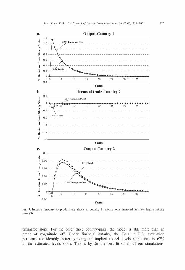
4.1.2. Low elasticity experiment
Heathcote and Perri (2002) make a case that the Armington elasticity is less than 1.
Lower Armington elasticities make the countries’ intermediate goods behave more like
complements, and less like substitutes, in the Armington aggregator. This would be
expected to raise comovement, as well as the responsiveness of comovement to changes in
trade intensity. The latter would arise to the extent that lower transport costs lead to a
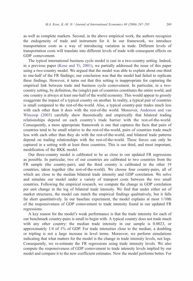
larger terms of trade movement in response to a TFP shock. Fig. 3 illustrates the impulse
response of the terms of trade and country 2’s output for the same case as Fig. 2, but with a
high Armington elasticity, 3. A comparison of the two figures shows that under a low
Armington elasticity the increase in the terms of a trade response to a TFP shock in
moving from 35% transport costs to free trade is larger than under a high Armington
elasticity.
We re-run our primary set of experiments with the elasticity Heathcote and Perri
use, 0.9. Table 3 reports the results under complete markets and financial autarky,
and computing both log and level slopes. The table shows that using lower
Armington elasticities does indeed improve the fit of the model; however, it still falls
short for both market structures and even with the levels slopes. Under complete
markets for example, the country-pair with an implied levels slope closest to the
estimated levels slope is Belgium–U.S., but the model slope is only about 21% of the
Output-Country 1
-0.2
0
0.2
0.4
0.6
0.8
1
1.2
1.4
0 5 10 15 20 25 30 35
Years
% D
evia
tion
fro
m S
tead
y St
ate
Free Trade
35% Transport Cost
Terms of trade-Country 2
-2
-1.6
-1.2
-0.8
-0.4
0
0.4
0 5 10 15 20 25 30 35
Years
% D
evia
tion
fro
m S
tead
y St
ate
Free Trade
35% Transport Cost
Output-Country 2
-0.02
0
0.02
0.04
0.06
0.08
0.1
0 5 10 15 20 25 30 35
Years
% D
evia
tion
fro
m S
tead
y St
ate
Free Trade
35% Transport Cost
a.
b.
c.
Fig. 3. Impulse response to productivity shock in country 1, international financial autarky, high elasticity
case (3).
M.A. Kose, K.-M. Yi / Journal of International Economics 68 (2006) 267–295 285
estimated slope. For the other three country-pairs, the model is still more than an
order of magnitude off. Under financial autarky, the Belgium–U.S. simulation
performs considerably better, yielding an implied model levels slope that is 67%
of the estimated levels slope. This is by far the best fit of all of our simulations.

Table 3
Quantitative assessment of effects of trade on GDP comovement, low elasticity experiment
Log slopes Estimated slope=0.091
Benchmark
country-pair
Transport
costs
Trade
intensity
Complete markets Financial autarky
GDP
correlation
Implied
slope
Implied
slope/
estimated
slope (%)
GDP
correlation
Implied
slope
Implied
slope/
estimated
slope (%)
Belgium U.S. 35% 0.00211 0.3607 0.3513
0% 0.00404 0.3658 0.0080 8.8 0.3676 0.0251 27.5
Australia Belgium 35% 0.00121 0.1886 0.1852
0% 0.00231 0.1893 0.0011 1.2 0.1865 0.0020 2.2
Finland Portugal 35% 0.00140 0.2881 0.3056
0% 0.00268 0.2893 0.0019 2.0 0.3067 0.0017 1.8
France U.S. 35% 0.00412 0.3579 0.3685
0% 0.00789 0.3603 0.0038 4.2 0.3792 0.0164 18.0
Level slopes Estimated slope=12.557
Benchmark
country-pair
Transport
costs
Trade
intensity
Complete markets Financial autarky
GDP
Correlation
Implied
slope
Implied
slope/
estimated
slope (%)
GDP
correlation
Implied
slope
Implied
slope/
estimated
slope (%)
Belgium U.S. 35% 0.00211 0.3607 0.3513
0% 0.00404 0.3658 2.681 21.4 0.3676 8.438 67.2
Australia Belgium 35% 0.00121 0.1886 0.1852
0% 0.00231 0.1893 0.642 5.1 0.1865 1.173 9.3
Finland Portugal 35% 0.00140 0.2881 0.3056
0% 0.00268 0.2893 0.941 7.5 0.3067 0.841 6.7
France U.S. 35% 0.00412 0.3579 0.3685
0% 0.00789 0.3603 0.652 5.2 0.3792 2.827 22.5
Implied slope in logs (levels) is calculated as change in GDP correlation per unit log (level) change in trade
intensity (between 35% and 0% transport costs).
M.A. Kose, K.-M. Yi / Journal of International Economics 68 (2006) 267–295286
However, again, in the other three country-pairs, the model explains 25% or less of
the empirical estimates.18
4.2. Two additional experiments
Our results suggest that the large gap between the model’s predictions and the empirical
evidence is certainly suggestive of a trade–comovement puzzle. However, in all of our
experiments until now, we have focused only on the channels directly linking bilateral
18 While the model performs relatively better with a low elasticity substitution, we note that such a low elasticity
is inconsistent with existing estimates–almost all of which are greater than our benchmark elasticity–and with
explaining large differences in trade across countries and over time. See Anderson and van Wincoop (2003),
Obstfeld and Rogoff (2001), and Yi (2003), for example. Hence, with respect to the volume of trade, the low
elasticity is counterfactual.
M.A. Kose, K.-M. Yi / Journal of International Economics 68 (2006) 267–295 287
trade to bilateral GDP correlations. In this section, we report on two experiments designed
to see if additional channels can help improve the fit to the data. The first experiment
examines a scenario in which all transport costs, not just those involving the country-pair
in question, change. However, we attribute all of the increase in GDP correlation only to
trade between the country-pair. The second experiment stems from the fact that TFP
correlation is closely related to bilateral trade intensity. In this experiment, we allow for the
correlation of TFP shocks to change when transport costs change.
4.2.1. All transport costs change
Many of the European countries in our sample share the same trading partners. Also,
for almost all countries, the U.S. is an important trading partner. It is possible, then, that
two small countries’ GDP’s are highly correlated because both trade heavily with the U.S.
and other countries. This channel would complement the direct bilateral channel. If pairs
of countries with higher bilateral trade intensity also tend to trade extensively with
common trading partners, then it is possible that the empirical estimates of the effect of
trade on GDP correlation suffer from a positive omitted variable bias.19 We assess the
possibility that the empirical estimates are upwardly biased by running simulations in
which transport costs between all three countries change simultaneously, and by
continuing to focus on the relationship between the two small countries’ bilateral trade
intensity and their GDP correlation. By doing so, we are essentially comparing pairs of
countries that trade heavily with each other and with the ROW to countries that trade little
with each other and with the ROW. As before, we calculate the change in GDP correlation
between the two small countries as the transport costs between them are varied, and
compare that against what would be predicted by the empirical estimates (based on the
change in the country-pair’s trade intensity).
Table 4 reports our results under financial autarky.20 The panel shows clearly that when
all transport costs decline simultaneously, the explanatory power of the model increases
substantially. Consider, for example, the Australia–Belgium benchmark case. Reducing all
transport costs from 35% to 0% raises the Australia–Belgium trade intensity from 0.00093
to 0.00248.21 The lower transport costs raise the GDP correlation from 0.0939 to 0.1645.
The implied log slope is 0.0716, which is 79% of our estimated slope of 0.091. Hence,
19 If there is a bias, one way to rectify this would be to construct a bilateral measure of intensity of trade with
common trading partners, and to re-estimate Eq. (1) including this variable in addition to the trade intensity
variable. However, it is likely that any such measure would be endogenous, and would need to be instrumented
for. It is unclear what instruments would be correlated with this measure, but uncorrelated with GDP
comovement. Among the cross-section and panel empirical papers, to our knowledge only Fidrmuc (2004)
attempts to control for common third-party trade. He enters a dummy variable for whether the pair of countries
belong to the EMU. He finds that the EMU countries tend to have higher comovement, all else equal.20 Under complete markets the responsiveness of GDP correlation to decreases in transport costs is non-
monotonic, rising when transport costs are high, but then declining when transport costs are low. We infer that the
resource-shifting channel associated with complete markets is more important at lower transport costs. Three of
our four benchmark country-pairs implied a negative relation between GDP comovement and trade (comparing
free trade and 35% transport costs).21 This is a smaller increase than in the first experiment, but is consistent with the insight from Anderson and van
Wincoop (2003) that bilateral trade flows depend on barriers relative to other countries. If all barriers fall, the
increase in (bilateral) trade is less than what would occur if only bilateral barriers fell.
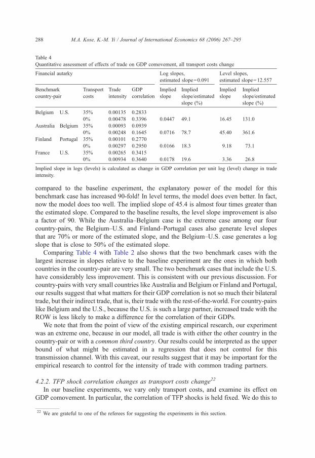
Table 4
Quantitative assessment of effects of trade on GDP comovement, all transport costs change
Financial autarky Log slopes,
estimated slope=0.091
Level slopes,
estimated slope=12.557
Benchmark
country-pair
Transport
costs
Trade
intensity
GDP
correlation
Implied
slope
Implied
slope/estimated
slope (%)
Implied
slope
Implied
slope/estimated
slope (%)
Belgium U.S. 35% 0.00135 0.2833
0% 0.00478 0.3396 0.0447 49.1 16.45 131.0
Australia Belgium 35% 0.00093 0.0939
0% 0.00248 0.1645 0.0716 78.7 45.40 361.6
Finland Portugal 35% 0.00101 0.2770
0% 0.00297 0.2950 0.0166 18.3 9.18 73.1
France U.S. 35% 0.00265 0.3415
0% 0.00934 0.3640 0.0178 19.6 3.36 26.8
Implied slope in logs (levels) is calculated as change in GDP correlation per unit log (level) change in trade
intensity.
M.A. Kose, K.-M. Yi / Journal of International Economics 68 (2006) 267–295288
compared to the baseline experiment, the explanatory power of the model for this
benchmark case has increased 90-fold! In level terms, the model does even better. In fact,
now the model does too well. The implied slope of 45.4 is almost four times greater than
the estimated slope. Compared to the baseline results, the level slope improvement is also
a factor of 90. While the Australia–Belgium case is the extreme case among our four
country-pairs, the Belgium–U.S. and Finland–Portugal cases also generate level slopes
that are 70% or more of the estimated slope, and the Belgium–U.S. case generates a log
slope that is close to 50% of the estimated slope.
Comparing Table 4 with Table 2 also shows that the two benchmark cases with the
largest increase in slopes relative to the baseline experiment are the ones in which both
countries in the country-pair are very small. The two benchmark cases that include the U.S.
have considerably less improvement. This is consistent with our previous discussion. For
country-pairs with very small countries like Australia and Belgium or Finland and Portugal,
our results suggest that what matters for their GDP correlation is not so much their bilateral
trade, but their indirect trade, that is, their trade with the rest-of-the-world. For country-pairs
like Belgium and the U.S., because the U.S. is such a large partner, increased trade with the
ROW is less likely to make a difference for the correlation of their GDPs.
We note that from the point of view of the existing empirical research, our experiment
was an extreme one, because in our model, all trade is with either the other country in the
country-pair or with a common third country. Our results could be interpreted as the upper
bound of what might be estimated in a regression that does not control for this
transmission channel. With this caveat, our results suggest that it may be important for the
empirical research to control for the intensity of trade with common trading partners.
4.2.2. TFP shock correlation changes as transport costs change22
In our baseline experiments, we vary only transport costs, and examine its effect on
GDP comovement. In particular, the correlation of TFP shocks is held fixed. We do this to
22 We are grateful to one of the referees for suggesting the experiments in this section.

Table 5
Quantitative assessment of effects of trade on GDP comovement, TFP correlations change
Complete markets Level slopes, estimated slope=12.557
Benchmark
country-pair
Transport
costs
Trade
intensity
GDP
correlation
Implied
slope
Implied
slope/estimated
slope (%)
Belgium U.S. 35% 0.00127 0.3235
0% 0.00500 0.3533 7.99 63.6
Australia Belgium 35% 0.00073 0.1450
0% 0.00286 0.1565 5.39 43.0
Finland Portugal 35% 0.00084 0.2506
0% 0.00331 0.2679 7.01 55.8
France U.S. 35% 0.00249 0.3419
0% 0.00974 0.3900 6.64 52.9
Financial autarky Level slopes, estimated slope=12.557
Benchmark
country-pair
Transport
costs
Trade
intensity
GDP
correlation
Implied
slope
Implied
slope/estimated
slope (%)
Belgium U.S. 35% 0.00127 0.3113
0% 0.00500 0.3479 9.82 78.2
Australia Belgium 35% 0.00073 0.1336
0% 0.00286 0.1456 5.59 44.5
Finland Portugal 35% 0.00084 0.2859
0% 0.00331 0.3040 7.30 58.1
France U.S. 35% 0.00249 0.3486
0% 0.00974 0.4016 7.32 58.3
Implied slope in logs (levels) is calculated as change in GDP correlation per unit log (level) change in trade
intensity.
M.A. Kose, K.-M. Yi / Journal of International Economics 68 (2006) 267–295 289
make our model simulations conform to the conditions underlying the empirical research.
Nevertheless, there may be another source of omitted variable bias in that increased trade
integration could be associated with increased TFP correlation. Recent evidence from the
trade and growth literature certainly supports this idea, at least for data at lower
frequencies.23 Moreover, our own data support this idea too. We re-run the regressions
from Section 2, except we replace GDP correlation with TFP correlation. The coefficient
in the levels regression is 13.08 (3.03).24 This is actually slightly larger than the estimated
coefficient in the GDP correlation regressions.25 This suggests that increased trade is
indeed associated with increased TFP comovement, or some force that looks like TFP
comovement.
We thus undertake an experiment in which, as transport costs decline, the correlation
between the TFP shocks in the two countries increases by an amount consistent with what
23 See Keller (2004) for a survey of international technology diffusion.24 The coefficient in the logs regression is 0.089 and the standard error on the coefficient is 0.017.25 We recognize that the apparent increase in TFP correlation associated with increased trade integration could
reflect forces such as variable factor utilization over the cycle. In this case, a more appropriate interpretation of
our measures of TFP are Solow residuals, which include both TFP and factor utilization.

M.A. Kose, K.-M. Yi / Journal of International Economics 68 (2006) 267–295290
is predicted by the TFP regressions.26 By doing so, we are essentially comparing pairs of
countries that trade heavily with each other and have high TFP shock correlations against
countries that trade little with each other and have low TFP shock correlations.
Consequently, as in the previous experiment, there are two forces driving comovement;
there is a direct effect from higher trade and an indirect effect resulting from trade’s effect
on TFP shock correlations. As before, we also attribute all changes in the GDP correlation
to variation in trade intensity.
Table 5 presents the results for blevelQ slope case. Under both complete markets and
financial autarky, the model performs much better. In all cases it explains at least 43% of
the estimated slopes. Under financial autarky, and for the Belgium–U.S. country-pair, the
model explains 78% of the estimated slope. Comparing these results to the bottom panel of
Table 2 shows that including for this indirect TFP correlation channel provides a
significant boost in the ability of the model to generate slopes close to those estimated in
the data.
Hence, like the experiment considered above, this experiment provides an alternative
explanation for why the empirical regressions yield a much greater responsiveness of
comovement to trade than our baseline exercise. It suggests that both the empirical
research and models might want to take this additional channel into account.
5. Conclusion
In this paper we examine whether the standard international business cycle
framework can quantitatively replicate the results of recent empirical research that finds
a positive association between the extent of bilateral trade and output comovement. We
employ a three-country business cycle model in which changes in transportation costs
induce an endogenous link between trade intensity and output comovement. On the face
of it, the model is expected to provide a good fit, because it embodies the key demand
and supply side spillover channels that are often invoked in explaining the trade-induced
transmission of business cycles. In particular, increased output in one country leads to
increased demand for the other country’s output. Following Heathcote and Perri (2002),
we study a model with international financial autarky, as well as complete markets.
Also, we calibrate our three-country model as closely as possible to the leading
empirical paper in the literature, Frankel and Rose (1998). The three-country aspect of
the model is important, because it captures the fact that most pairs of countries are small
relative to the world.
We find that the standard international business cycle model is able to capture the
positive relationship between trade and output comovement, but our baseline experiment
falls far short of explaining the magnitude of the empirical findings. This is true even
when we control for the fact that bilateral trade between countries is typically quite
26 Specifically, the decline in transport costs implies an increase in steady-state trade. That increase in trade is
associated with a particular increase in TFP correlation, according to the regression estimates. We adjust the
correlation of the TFP shocks to produce that increase in the TFP correlation.

M.A. Kose, K.-M. Yi / Journal of International Economics 68 (2006) 267–295 291
small as a share of GDP and relative to a country’s total trade by computing level
slopes, as opposed to the log slopes that are typically estimated in the empirical
research. Another reason for the model’s failure has to do with feedback effects from the
country-pair to the world economy and then back. Even country-pairs with large
absolute changes in their bilateral trade share of GDP will not generate large feedback
effects if the pair constitutes a small share of world GDP. In this sense, we have
identified a trade–comovement puzzle.
Our trade–comovement puzzle is different from the six puzzles in international
macroeconomics that Obstfeld and Rogoff (2001) identify. The two puzzles most closely
related to ours are the consumption correlations puzzle and the home-bias-in-trade puzzle.
As discussed earlier, the consumption correlations puzzle is a puzzle about levels and
rankings of cross-country consumption and output correlations. The home-bias-in-trade
puzzle is about explaining low levels of trade. Our problem is about the responsiveness of
output correlations to changes in bilateral trade. It is about slopes, not levels, of
correlations. We do not seek to explain the low levels of trade; rather, we take these levels
as given, and ask how variation in them affects output correlations.
We conduct two further experiments that might help explain the empirical findings. In
one experiment, we vary all transport costs, not just those between the country-pair, but we
attribute all of the correlation changes to change in the country-pair’s bilateral trade. This
experiment allows us to obtain a slope that is closer to, and in some cases, exceeds, the
estimated slopes. This suggests that the empirical research might benefit from controlling
for intensity of third-party trade. In addition, we conduct an experiment in which as
transport costs decline, and trade increases, the correlation of TFP shocks increases, as
well. With two channels affecting GDP correlation, the pure trade channel, and an indirect
channel operating through TFP comovement, it is not surprising that the model does a
much better job in this experiment. Both of these experiments suggest additional control
variables for the empirical research. Our empirical finding that TFP comovement is
strongly positively associated with trade suggests a puzzle for model builders, as well. We
leave this for future research.
In their empirical work, FR do not control for variables other than bilateral trade
intensity. Other researchers, especially Imbs (2004), contend that controlling for sectoral
similarity in the regressions leads to smaller coefficients on trade. However, Baxter and
Kouparitsas (2004), Calderon et al. (2002), Clark and van Wincoop (2001), and Otto et al.
(2001) also control for industrial or sectoral similarity (among other variables) and the
coefficients on trade are still statistically significant. An additional empirical finding is that
intra-industry trade is more important than inter-industry trade or total trade in driving
GDP comovement.27 We would suggest addressing the importance of these sectoral issues
from the lens of a dynamic stochastic general equilibrium model. Indeed, there are models
that include multiple sectors, including those by Kouparitsas (1998) and Ambler et al.
(2002). Also, Burstein et al. (2004) implement a version of a multiple sector model with
27 See, for example, Fidrmuc (2004), Shin and Wang (2004), and Gruben et al. (2002). Allowing for increased
specialization poses a double-edged sword, however. To the extent that it generates less industrial similarity
across countries, and to the extent that industry-specific shocks are important drivers of the business cycle, then
increased specialization could reduce output comovement.
M.A. Kose, K.-M. Yi / Journal of International Economics 68 (2006) 267–295292
production sharing. A further extension would be to replace the Armington aggregator in
these models, in which specialization patterns are invariant to changing trade costs, with
neoclassical trade theory, in which specialization patterns can endogenously change when
trade costs change.
Acknowledgements
The previous version of this paper circulated under the title bThe Trade-Comovement
Problem in International Macroeconomics. We thank two anonymous referees for
extremely helpful comments that greatly improved the paper. We also thank Julian de
Giovanni, Tim Kehoe, Narayana Kocherlakota, Michael Kouparitsas, Paolo Mauro,
Fabrizio Perri, Linda Tesar, Eric van Wincoop, Christian Zimmermann, and participants at
the 2002 Growth and Business Cycle Theory Conference, the Spring 2002 Midwest
International Economics Meetings, Korea University, and at the IMF Research Department
brown bag for useful comments. Mychal Campos, Matthew Kondratowicz, Edith Ostapik,
and Kulaya Tantitemit provided excellent research assistance. The views expressed in this
paper are those of the authors and are not necessarily reflective of views of the
International Monetary Fund, the Federal Reserve Bank of Philadelphia, or the Federal
Reserve System.
Appendix A. Productivity shock process and import shares
A.1. Estimating productivity shock process
Our raw data for computing the productivity shocks comes from the Penn World
Tables, version 6.0. For the period 1970–1998, we obtain data on population, real GDP
(chained), and real GDP per worker for the 21 countries in our sample. For each simulation
involving a particular country-pair, we calculate three sets of Solow residuals. The first
two sets correspond to the two countries in the country-pair. The third set corresponds to
the other 19 countries, which serve as the rest-of-the-world (ROW). Output and labor are
summed across countries to yield a ROW aggregate. The Solow residuals are constructed
as follows:
Zit ¼ ln Yitð Þ � 0:64ln Litð Þ ð20Þ
where Yit is real GDP for country i in year t, and Lit is the number of workers in country
i in year t. Our coefficient on labor corresponds to the labor share of output used by
BKK, for example. The capital stock data in the latest Penn World Tables are currently
not available.
With the three sets of Solow residuals, we estimate an AR1 productivity shock matrix
A. We regress each set of residuals on a constant, a time trend, and lagged values of each
of the three residuals. This yields the A matrices listed in Appendix Table 1. The standard
deviations and correlation matrix of the residuals are used to construct the variance–
covariance matrix V of the residuals; these values are also listed in Appendix Table 1.

Appendix Table 1
Estimated productivity shock process and import shares
Belgium–U.S. Australia–Belgium Finland–Portugal France–U.S.
A matrix (matrix of AR1 productivity shocks)
Belgium U.S. ROW Australia Belgium ROW Finland Portugal ROW France U.S. ROW
Belgium 0.513 0.352 0.074 Austral. 0.731 �0.143 �0.317 Finland 0.669 �0.189 0.396 France 0.581 0.241 0.020
U.S. �0.168 0.823 �0.464 Belgium 0.197 0.436 0.421 Portugal �0.244 0.562 1.018 U.S. �0.296 0.762 �0.293ROW �0.252 0.197 0.771 ROW 0.108 �0.303 0.783 ROW �0.071 �0.133 0.829 ROW 0.025 0.268 0.432
Standard deviation of residuals
Belgium U.S. ROW Australia Belgium ROW Finland Portugal ROW France U.S. ROW
0.016 0.018 0.011 0.018 0.016 0.013 0.031 0.029 0.013 0.012 0.018 0.012
Correlation of residuals
Belgium U.S. ROW Australia Belgium ROW Finland Portugal ROW France U.S. ROW
Belgium Austral. Finland France
U.S. 0.368 Belgium 0.248 Portugal 0.125 U.S. 0.438
ROW 0.577 0.684 ROW 0.461 0.516 ROW 0.339 0.496 ROW 0.670 0.694
Matrix of import shares
To From To From To From To From
Belgium U.S. ROW Australia Belgium ROW Finland Portugal ROW France U.S. ROW
Belgium 0.359 0.047 0.594 Austral. 0.830 0.002 0.168 Finland 0.721 0.003 0.277 France 0.792 0.022 0.186
U.S. 0.002 0.899 0.099 Belgium 0.003 0.359 0.638 Portugal 0.002 0.649 0.349 U.S. 0.004 0.899 0.097
ROW 0.024 0.074 0.901 ROW 0.014 0.047 0.940 ROW 0.035 0.019 0.946 ROW 0.038 0.072 0.890
Data sources include Penn World Tables, version 6.0; and the IMF’s Direction of Trade Statistics.
M.A.Kose,
K.-M
.Yi/JournalofIntern
atio
nalEconomics
68(2006)267–295
293
M.A. Kose, K.-M. Yi / Journal of International Economics 68 (2006) 267–295294
A.2. Calculating import shares
We calibrate the Armington aggregator parameters so that under transportation costs of
15% the implied steady-state import shares match the actual import shares, and
intermediate goods output equals final goods output.28 Specifically, for each set of three
countries (the specified country-pair and the rest-of-the-world) there are nine aggregator
parameters to set. We use two first-order conditions from final goods firm j’s maximization
problem, (six equations in total), where the actual import shares enter in the expression in
parentheses on the right-hand side below:
pij
pj
� �1�a
¼ xij
xjj
pjyjj=yjpijmij=yj
� �a
: ð21Þ
We also set intermediate goods output equal to final goods output, as in Backus et al.
(1992), (three equations) to determine the nine parameters. These nine equations must be
solved along with the other steady-state equations of the model.
We follow Zimmermann (1997) by calculating the import shares, e.g. ( pijmij)/( yj), for
each trading partner of each of the three countries. This is complicated by the fact that
imports by ROW countries from other ROW countries are in our framework redundant or
internal trade, and need to be subtracted from the raw imports data. Then, for each country,
we divide the import share of GDP (with ROW imports appropriately adjusted) among the
two other countries according to their share in the country’s imports from these two
countries. Imports from the own country are defined as 1-import share of GDP (again, with
ROW imports appropriately adjusted).
References
Ambler, Steve, Cardia, Emanuela, Zimmerman, Christian, 2002. International transmission of the business cycle
in a multi-sector model. European Economic Review 46, 273–300.
Anderson, James, van Wincoop, Eric, 2003. Gravity with gravitas: a solution to the border puzzle. American
Economic Review, March 93, 170–192.
Anderson, Heather, Kwark, Noh Sun, Vashid, Farhid, 1999. Does International Trade Synchronize Business
Cycles? Manuscript, Monash University and Texas A&M University, July 1999.
Backus, David K., Kehoe, Patrick J., Kydland, Finn E., 1992. International real business cycles. Journal of
Political Economy, August 100 (4), 745–775.
Backus, David K., Kehoe, Patrick J., Kydland, Finn E., 1994. Dynamics of the trade balance and the terms of
trade: the J-curve? American Economic Review 84 (1), 84–103 (March).
Baier, Scott, Bergstrand, Jeffrey H., 2001. The growth of world trade: tariffs, transport costs, and income
similarity. Journal of International Economics 53, 1–28.
Baxter, Marianne, Crucini, Mario, 1995. Business cycles and the asset structure of foreign trade. International
Economic Review 36, 821–854.
Baxter, Marianne, Kouparitsas, Michael, 2004. Determinants of Business Cycle Comovement: A Robust
Analysis. NBER Working Paper 10725, August 2004.
Betts, Caroline M., Kehoe, Timothy J., 2001. Tradability of Goods and Real Exchange Rate Fluctuations.
Manuscript, University of Southern California and University of Minnesota.
28 In Kose and Yi (2002), we calibrated the aggregator parameters so that the steady-state import shares match
the actual import shares under free trade. The results are virtually identical.
M.A. Kose, K.-M. Yi / Journal of International Economics 68 (2006) 267–295 295
Burstein, Ariel, Kurz, Johann, Christopher, Tesar, Linda, 2004. Trade, Production Sharing, and the International
Transmission of Business Cycles. Manuscript, UCLA and University of Michigan, November.
Calderon, Cesar A., Chong, Alberto E., Stein, Ernesto H., 2002. Trade Intensity and Business Cycle
Synchronization: Are Developing Countries any Different? Manuscript, Inter-American Development Bank,
March.
Canova, Fabio, Harris, Dellas, 1993. Trade interdependence and the international business cycle. Journal of
International Economics 34, 23–47.
Clark, Todd E., van Wincoop, Eric, 2001. Borders and business cycles. Journal of International Economics 55,
59–85.
Fidrmuc, Jarko, 2004. The endogeneity of the optimum currency area criteria, intra-industry trade, and EMU
enlargement. Contemporary Economic Policy, January 22 (1), 1–12.
Frankel, Jeffrey A., Rose, Andrew K., 1998. The endogeneity of the optimum currency area criteria. Economic
Journal, July 108, 1009–1025.
Gruben, William C., Koo, Jahyeong, Millis, Eric, 2002. Does International Trade Affect Business Cycle
Synchronization?, Manuscript, Federal Reserve Bank of Dallas, November.
Head, Allen, 2002. Aggregate fluctuations with national and international returns to scale. International Economic
Review, November 43 (4), 1101–1125.
Heathcote, Jonathan, Perri, Fabrizio, 2002. Financial autarky and international business cycles. Journal of
Monetary Economics, April 49 (3), 601–628.
Hummels, David, Ishii, Jun, Yi, Kei-Mu, 2001. The nature and growth of vertical specialization in world trade.
Journal of International Economics, June 54, 75–96.
Imbs, Jean, 2004. Trade, finance, specialization, and synchronization. Review of Economics and Statistics,
August 86 (3), 723–734.
Keller, Wolfgang, 2004. International technology diffusion. Journal of Economic Literature, September 42 (3),
752–782.
Kose, M. Ayhan, Yi, Kei-Mu, 2001. International trade and business cycles: is vertical specialization the missing
link? American Economic Review, Papers and Proceedings 91, 371–375.
Kose M. Ayhan, Yi, Kei-Mu, December 2002. The Trade–Comovement Problem in International Macroeco-
nomics, Federal Reserve Bank of New York Staff Report #155.
Kouparitsas, Michael, April 1998. North–South Business Cycles. Manuscript, Federal Reserve Bank of Chicago.
Mazzenga, Elisabetta, Ravn, Morton O., 2004. International business cycles: the quantitative role of
transportation costs. Journal of International Money and Finance 23, 645–671 (August).
Obstfeld, Maurice, Rogoff, Kenneth, 2001. The six major puzzles in international macroeconomics: is there a
common cause? NBER Macroeconomics Annual 2000, pp. 339–389.
Otto, Glenn, Voss, Graham, Willard, Luke, 2001. Understanding OECD Output Correlations, RDP 2001–05.
Reserve Bank of Australia.
Prasad, Eswar S., 1999. International trade and the business cycle. Economic Journal, October 109, 588–606.
Ravn, Morton O., Mazzenga, Elisabetta, 1999. Frictions in International Trade and Relative Price Movements.
Manuscript, London Business School.
Ravn, Morton O., Mazzenga, Elisabetta, 2004. International business cycles: the quantitative role of
transportation costs. Journal of International Money and Finance 23, 645–671.
Schmitt-Grohe, Stephanie, 1998. The international transmission of economic fluctuations: effects of U.S. business
cycles on the canadian economy. Journal of International Economics 44, 257–287.
Shin, Kwanho, Wang, Yunjong, 2004. Trade integration and business cycle co-movements: the case of Korea with
other Asian Countries. Japan and the World Economy 16, 213–230.
Yi, Kei-Mu, 2003. Can vertical specialization explain the growth of world trade? Journal of Political Economy,
February, 52–102.
Zimmermann, Christian, 1997. International real business cycles among heterogeneous countries. European
Economic Review 41, 319–355.