Can Productivity Increases Really Explain The Lira

Loyola University Chicago Loyola University Chicago

Loyola eCommons Loyola eCommons

Topics in Middle Eastern and North African Economies Journals and Magazines

9-1-2012

Can Productivity Increases Really Explain The Lira Appreciation: Can Productivity Increases Really Explain The Lira Appreciation:

Questions For The Central Bank Of The Republic Of Turkey Questions For The Central Bank Of The Republic Of Turkey

Kenan Lopcua Çukurova University

Almila Burgacb Çukurova University

Fikret Dulger Çukurova University

Follow this and additional works at: https://ecommons.luc.edu/meea

Part of the Economics Commons

Recommended Citation Recommended Citation Lopcua, Kenan; Burgacb, Almila; and Dulger, Fikret, "Can Productivity Increases Really Explain The Lira Appreciation: Questions For The Central Bank Of The Republic Of Turkey". Topics in Middle Eastern and North African Economies, electronic journal, 14, Middle East Economic Association and Loyola University Chicago, 2012, http://www.luc.edu/orgs/meea/

This Article is brought to you for free and open access by the Journals and Magazines at Loyola eCommons. It has been accepted for inclusion in Topics in Middle Eastern and North African Economies by an authorized administrator of Loyola eCommons. For more information, please contact [email protected]. © 2012 the authors

https://ecommons.luc.edu/

https://ecommons.luc.edu/meea

https://ecommons.luc.edu/meea

https://ecommons.luc.edu/periodicals

https://ecommons.luc.edu/meea?utm_source=ecommons.luc.edu%2Fmeea%2F163&utm_medium=PDF&utm_campaign=PDFCoverPages

http://network.bepress.com/hgg/discipline/340?utm_source=ecommons.luc.edu%2Fmeea%2F163&utm_medium=PDF&utm_campaign=PDFCoverPages

http://www.luc.edu/orgs/meea/

mailto:[email protected]

Topics in Middle Eastern and African Economies

Vol. 14, September 2012

311

CAN PRODUCTIVITY INCREASES REALLY EXPLAIN THE LIRA

APPRECIATION: QUESTIONS FOR THE CENTRAL

BANK OF THE REPUBLIC OF TURKEY

Kenan LOPCUa Almıla BURGAÇ

b Fikret DÜLGER

c

Çukurova University, Turkey

Prepared for presentation at the 32nd

Annual Meeting of the MEEA, ASSA

January 5-8, 2012, Chicago, IL

Abstract

This paper studies the Balassa-Samuelson (B-S) hypothesis between Turkey and 27

members of the European Union (EU-27). The Central Bank of the Republic of Turkey

(CBRT) in recent years has emphasized the importance of the B-S hypothesis for Turkey.

Specifically, the CBRT states that structural reforms, increased confidence, and

macroeconomic stability in the post 2001 era have contributed to the strengthening of the

national currency through the relative price differentials between tradable versus non-tradable

goods (Inflation Report II, 2006, pp: 31-34). Given this emphasis by the CBRT, we test the

cointegrating relationship between the real effective exchange rate, relative productivity, real

interest rate differentials and the net foreign asset, using recently developed cointegration

techniques with multiple structural breaks. The findings reveal that the relative productivities

play a limited role in explaining the real effective exchange rate appreciation. In particular,

the relationship between the real effective exchange rate and productivity is not supported for

the post 2001 era.

Keywords: Balassa-Samuelson Hypothesis, Real Effective Exchange Rate, Relative

Productivity, Cointegration, Multiple Structural Breaks

JEL Codes: C22, E31, F31

a Corresponding author. [email protected], Department of Econometrics, Çukurova University, Balcalı, Adana

01330, Turkey

[email protected], Department of Economics, Çukurova University, Balcalı, Adana 01330, Turkey

[email protected], Department of Economics, Çukurova University, Balcalı, Adana 01330, Turkey




Topics in Middle Eastern and African Economies Vol. 14, September 2012

312

Introduction

The Balassa-Samuelson (B-S) hypothesis relies on the productivity differentials

between tradable and non-tradable sectors to explain deviations in purchasing power parity.

According to the B-S hypothesis, because productivity growth in tradable sectors is higher

than in non-tradable sectors, real wages increase in tradable sectors. On the other hand,

because the prices of tradable goods are determined in the world market, tradable prices will

not increase. With an assumption of perfect labor mobility within a country, increases in

wages in tradable sectors will be reflected in non-tradable sectors as well. However, an

increase in wages in non-tradable sectors is not accompanied by an increase in productivity.

As a result, the prices of non-tradable goods will increase, leading to an increase in the overall

price level and the appreciation of the real exchange rate for the domestic economy. Thus,

within this framework, the relative productivity differences in tradable vis-à-vis non-tradable

sectors between two countries will determine the long-run changes of the real exchange rate.

The Central Bank of the Republic of Turkey (CBRT) in recent years has emphasized

the importance of the Balassa-Samuelson hypothesis for Turkey. Specifically, co-observance

of the Turkish lira’s tendency to appreciate and the price differentials between tradable and

non-tradable sectors necessitates a close investigation of the relationship between the real

exchange rate and price differentials. In this regard, part of the appreciation of the Turkish lira

(TL) can be attributed to the productivity differentials between tradable and non-tradable

sectors. In particular, in addition to the direct effects of structural reforms undertaken after

the 2001 crisis, increased confidence, optimism, and macroeconomic stability in recent years

have contributed to the strengthening of the national currency through the relative price

differentials between tradable versus non-tradable goods (Inflation Report II, 2006).

The main purpose of this study then, given the increased consideration of the Balassa-

Samuelson effect by the CBRT, is to test whether part of the appreciation of the TL is driven

by the relatively rapid productivity increases in the tradable sectors in recent years. Hence, the

study examines the validity of the B-S hypothesis between Turkey and 27 member countries

of the European Union (EU-27), which includes the majority of Turkey’s main trading

partners, for the post-financial liberalization era, using recently developed cointegration

techniques with multiple structural breaks.

The paper consists of five sections, including the introduction. Section two presents

the theoretical framework of the B-S hypothesis and reviews the literature. In section three,


313

the data and the empirical method used to test the B-S hypothesis are explained. Section four

presents the empirical finding, and section five concludes.

Theoretical Framework

There are several possible theoretical explanations in the literature for the real

exchange rate movements. One of the most important models of long-run deviations from the

purchasing power parity (PPP) was developed by Balassa (1964) and Samuelson (1964). They

explained that relative productivity differences across countries cause the real exchange rate

to deviate from the PPP in the long run. A rapid productivity increase in the tradable sector

vis-à-vis the non-tradable sector in the home country in relation to the rest of the world will

cause the aggregate price level to increase faster and consequently cause the home currency to

appreciate.

In other words, an increase in productivity in the tradable sector will cause an increase

in real wages in that sector. Given the perfect labor mobility within a country, increases in

wages in tradable sectors will also increase the wages in non-tradable sectors. However, this

increase in wages in non-tradable sectors is not supported by an increase in productivity.

Hence, the prices of non-tradable goods will increase, pushing the aggregate price level up,

thereby leading to the appreciation of the real exchange rate for the home country.

The basic features of the B-S hypothesis were first described by Samuelson (1964),

and empirically tested by Balassa (1964). The functioning of the model relies on some basic

assumptions: the PPP holds for tradables; labor productivity determines wages in the tradable

sector; labor is not mobile between countries but perfectly mobile within a country, which

causes the wages to match between sectors within the home country; and finally, there is

perfect capital mobility within and between countries.

Consider a small economy that produces output in tradable and nontradable sectors,

using constant returns to scale technology with capital and labor1:

1)()( TTTT KLAY (1)

1)()( NTNTNTNT KLAY (2)

Where T and NT denote the tradable and non-tradable sectors, Y is output level, and A,

L, and K are technology, labor, and capital, respectively. γ and δ denote the share of labor in

1 Obstfeld and Rogoff, 1996, 204-216


314

the tradable and non-tradable sectors. Assuming the perfect mobility of factors of production,

the profit maximization under the perfect competition yields:

1)/( TTT LKAW (3)

1)/()/(TNNTNTTNT LKAPPW (4)

)/)(1( TTT LKAR (5)

)/)(1()/( NTNTNTTNT LKAPPR (6)

Where W and R reflect the wage rate and the interest rate, respectively. The interest

rate is determined in the world market. PNT / PT is the relative price of non-tradables in term

of tradables. Taking the logarithms, totally differentiating, and rearranging equations (3-6)

yields the domestic version of the B-S hypothesis:

NTTTNT dada)/()pp(d (7)

NTTTNT aa)/(cons)pp( . (7a)

Where, cons stands for constant.

Equation (7) indicates that given the equal factor intensities in the tradable and non-

tradable sectors (δ = γ), faster productivity increases in the tradable sector will cause higher

prices in the non-tradable sector than those of the tradable sector. The assumption of equal

factor intensity is sufficient but not even necessary to reach this conclusion from equation (7).

Since the labor intensity is likely to be higher in the non-tradable sector (δ > γ), even a mild

productivity increase in favor of the tradable sector can generate a higher relative price for the

non-tradable sector (Ègert, Halpern and MacDonald, 2006; Kravis and Lispey 1982;

Bhagwathi, 1984). Hence, the relative productivity-price relationship in (7) may alternatively

be expressed as

NTTTNT aafpp (7b)

Assuming that the factor intensities are the same for the domestic, and foreign

economies (δ = γ and δ* = γ*), then the relationship between the relative price and relative

productivity differences between the domestic and foreign economies can be written as

follows.

*

NT

*

TNTT

*

T

*

NTTNT aaaaconspppp (7c)

Equation (7c) reflects the international transmission mechanism of the B-S hypothesis.

It explains why the increase in relative productivity of the tradable sector vis-à-vis the non-

tradable sector for the domestic economy compared to the foreign economy leads to an

appreciation of the domestic currency. An increase in the relative productivity of the tradables


315

leads to an increase in the prices of non-tradables. This in turn increases the aggregate price

level for the domestic economy, causing appreciation of the domestic currency.

The real exchange rate can be expressed as the nominal exchange rate times the

domestic price level divided by the foreign price level:

*/ PEPQ (8)

Where, P* and P denote foreign and domestic price levels, and Q and E reflect the real

and nominal exchange rates. In foreign and domestic economies, the general price level is

expressed by the weighted average of tradable and non-tradable goods.

1

NTT PPP (9)

** 1*** NTT PPP (9a)

Where, PT and PT* represent the price levels of tradables in home and foreign country;

while PNT and PNT*

reflect the price level of non-tradables in the home and foreign country,

respectively. α and α* are shares of the tradable goods in the aggregate price level in home

and foreign country.

Assuming that equation (7c) holds and α=α*, taking the natural logarithms of equations

(8, 9, 9a), and then substituting (9 and 9a) into equation (8), yields equation (10).

*** )1()( NTtTtNTtTtTtTttt aaaappeconsq (10)

TtNTtTtt qqconsq , (10a)

The second term in equation (10), Ttq , is the PPP for tradable goods. It is equal to zero

if PPP holds for the tradable sector, so, equation (10) can be rewritten as

**)1( NTtTtNTtTtt aaaaconsq (10b)

Equation (10b) is the standard B-S hypothesis and is purely supply sided and hence

fairly restrictive. We relax the assumption of PPP for tradables to be true all the time and

focus on balance of payments to explain deviations in it. Given the floating exchange rate

regime and assuming no intervention in the exchange rate market, the equilibrium condition

for balance of payments would hold (Kanamori and Zhoa, 2006).

0t tca ka (11)

cat and kat in equation (11) are the current account and capital account, respectively.

Assuming that the current account in period t is determined by net exports, nxt and interest

earnings (payments) on net foreign assets, nfat, we have

tttt nfanxca (12)


316

Where denotes the real lending (borrowing) rate for the home country while the

term, tt nfa represents the net real interest payments (earnings) for the domestic economy.

We are assuming the real lending (borrowing) rate to be constant for the domestic economy

and ignoring some other minor components that might influence the current account in

equation (12). Next, we turn to the determinants of net exports and assume that changes in

the real exchange rate or terms of trade, an indicator of competitiveness, have an effect on net

exports and the current account. Open economy macroeconomics also suggests that domestic

and foreign incomes also have an impact on net exports. The former worsens net exports by

stimulating imports while the latter improves net exports via increasing the demand for

domestically produced goods abroad. Hence, the following standard relationship for net

exports is proposed.

*

32

*

1 )( ttTtTttt yyppenx (13)

Where et is the nominal exchange rate, Ttp and *

Ttp are the log domestic and foreign

price levels, respectively, for tradables, and ty and *

ty denote the log of the real domestic and

foreign income levels in that order. i , for i=1,2,3 are the elasticities with respect to the real

exchange rate, and real domestic and foreign incomes correspondingly at time t.

Turning to the second component of balance of payments, we presume that the capital

account is determined by the following relationship.

)( 1

* e

tttt eiika (14)

The term in parenthesis is the uncovered interest rate parity, where it and *

ti represent

the domestic and foreign nominal interest rate correspondingly, and e

te 1 is the expected

change in the nominal exchange rate. Uncovered interest rate parity does not necessarily hold

all the time. However, when there are deviations from the parity, appropriate flows of capital

will tend to establish the parity again. Specifically, an increase in the home country interest

rate will attract international capital and cause the exchange rate to appreciate, while a rise in

the foreign interest rate will reduce capital inflow, causing the expected value of domestic

currency to depreciate and thus stimulate capital outflow. Hence, assuming the combined

impacts of domestic and foreign income levels in equation (13) to be constant (at least fairly

stable), the balance of payments nominal exchange rate equation can be written (or

approximated) as

)()( 1

*

11

* e

ttttTtTtt eiinfappconse

(15)


317

Equation (15) can be thought of as a general formulation, corresponding to the

equilibrium exchange rate. It is compatible with the balance of payments equilibrium under

the floating exchange rate regime. Given that the expected change in the exchange rate can be

proxied by the home and foreign expected inflation differentials, equation (15) can be

rewritten as follows.

)()()( *

11

*

tttTtTtt rrnfappconse

(15a)

For tradable goods the real exchange rate is defined as follows.

*

TtTttTt ppeq (16)

Hence, we can write the real exchange rate for tradables at time t as follows.

)( *

11

tttTt rrnfaconsq

(17)

Where rt and rt*

reflect real interest rate in home and foreign country at time t.

Substituting equation (17) in equation (10) we obtain

***

11

)1()( NTtTtNTttTtttt aaaarrnfaconsq

(18)

or in compact form, we have

),,( *

ttttt rrnfaprodfq (18a)

Equation (18) is our real exchange rate model, indicating that the real exchange rate is

a function of relative productivity differentials, net foreign assets and real interest rate

differentials. Equation (18) is completely compatible with equation (5) in Clark and

MacDonald (2000).

We study several variations of this model based on the combinations of net foreign

assets and real interest rate differentials in addition to relative productivities. In particular,

according to the specific to general principle, the following fundamental determinants of the

real exchange rate are employed as independent variables in the empirical models analyzed.

Model 1a: ttt uprodconsreer 1

Model 1b: tttt uprodeuprodtrconsreer 21

Model 2a: tttt unfaprodconsreer 21

Model 2b: ttttt unfaprodeuprodtrconsreer 321

Model 3a: tttt urirprodconsreer 21


318

Model 3b: ttttt urirprodeuprodtrconsreer 321

Model 4: ttttt urirnfaprodconsreer 321

Where prodtr and prodeu stand for relative productivities in the tradable and non-

tradable sectors in Turkey and EU27, respectively; rir describes real interest rate differentials

between Turkey and EU27; prod is relative productivity differentials, prodtr-prodeu ; and nfa

is net foreign assets of the home country.

Literature Review

There is a large body of empirical literature dealing with changes in the real exchange

rate. Table 1 presents some selected empirical studies with time period, variables used, proxy

for productivity, method and the effect of productivity on the real exchange rate.

Alberola et. al (1999) investigated the relationship between the real exchange rate and

fundamentals of its external and internal components (stock of the net foreign assets and

relative sectoral prices) for the United States (US), Japan Canada, and the EU countries for

the 1980:Q1- 1998:Q4 period, using panel cointegration methods. They found the coefficient

of relative price differentials (proxy for the B-S effect) to be significant and circa unity as

theoretically expected.

MacDonald and Nagayasu (2000) investigated the long-run relationship between the

real exchange rate and the real interest rate differential for 14 industrialized countries for the

period of 1976-1997. Using panel cointegration tests, they found that the estimated slope

coefficients were consistent with the model and that there was a long-run relationship between

real exchange rate and real interest rate differentials.

Rahn (2003) estimated the real exchange rate for five EU accession countries by

applying the Behavioral Equilibrium Exchange Rate (BEER) and Permanent Equilibrium

Exchange Rate (PEER) approach, using quarterly data from 1990:Q1 to 2002:Q1. Both

Johansen and panel cointegration techniques revealed that the impacts of productivity

differences and net foreign assets on the real exchange rate were positive and significant.

MacDonald and Wojcik (2004) examined the exchange rate behavior of four

transitional and EU accession economies, with panel DOLS for the period from 1995 to 2001.

They found that the B-S effect led to modest appreciation of the real exchange rate with an

elasticity not exceeding 0.51. The results were robust to various changes in the model, such as

adding supply and demand effects, and real wages in addition to real interest rate differentials

and net foreign assets, and all the macroeconomic variables had correct signs (positive) and


319

were statistically significant. For related group countries, Alberola and Navia (2008) focused

on the role of capital flows and the B-S hypothesis to determine the real exchange rate for

new EU members. The authors concluded that the real exchange rate appreciated with

productivity growth, and productivity gains improved competitiveness without the need for

the exchange rate adjustment.

Table1. Selected Empirical Studies for Testing the B-S Hypothesis

Author(s) Country Period Independent

Variables

Productivity

Proxy

Method Sign

(B-S)

Balassa (1964) 12 1960 GDP GDP OLS +

Alberola et al.

(1999) 11 1980-1998 Prod, nfa CPI/WPI Panel +

Clark and

MacDonald (2000) 3 1960-1997 Prod, nfa, rir CPI/WPI

VECM,

Johansen +,-

Rahn (2003) 5 1990-2002 Prod, nfa CPI/WPI Johansen,

Pedroni

+

MacDonald and

Ricci (2003)

South

Africa 1970-2001

Prod, rir, open,

nfa, fb, GDP Johansen +

Lommatzsch and

Tober (2004) 3 1994-2003 Prod, debt, r, Y/L E-G +, -

Lane and Milesi-

Ferretti (2004) 64 1970-1997 Prod, tot, nfa GDP DOLS +

MacDonald and

Wojcik (2004) 4 1995-2001 Prod, nfa, rir Y/L PDOLS +

Égert (2005) 6 1985-2004 at-an Y/L ARDL,

DOLS +

MacDonald and

Ricci (2005) 10 1970-1991

Prod, nfa , at, an,

ad, rir TFP DOLS +

Gente (2006) 6 1970-1992 at, an, rir TFP Calibration +

Alberola and Navia

(2008) 3 1993-2004 Prod, nfa Y/L Johansen +

Mejean (2008) 16 1981-1999 Prod, nfa, ulc, sa Y/L Pedroni -

Coudert and

Couharde (2009) 128 1974-2004 Prod, nfa GDP Pedroni +

Camarero (2008) 12 1970-1998 at, an, ad, nfa, rir,

pe. Y/L PMGE +

Bénassy-Quéré et

al, (2010) 15 1980-2005 Prod, nfa, tot CPI/WPI Panel -

Alper and Civcir

(2012) Turkey 1987-2010 Y/L, nfa Y/L Johansen +

ARDL: Autoregressive Distributed Lag; at: Relative productivity in tradables; an: Relative productivity in nontradables; ad: Relative

productivity in the distribution sector; CPI: Consumer price index; debt: Total foreign debt; E-G: Engle Granger Cointegration Method; fb: Ratio of fiscal balance to GDP; GDP: Real GDP per capita; nfa: Ratio of net foreign assets to GDP; OLS: Ordinary Least Squares; open:

Openness; pe: Public expenditure; PDOLS: Panel Dynamic Ordinary Least Squares; PMGE: Pooled Mean Group Estimation; p.oil: Price

of oil, prod: Relative productivity differentials; r: Real interest rate; rir: Real interest rate differentials; sa: Supplier access; tot: Terms of trade; ulc Unit labor cost; VECM: Vector Error Correction Model; Y/L: Average labor productivity; WPI: Producer price index.

Camarero (2008) examined the role of productivity in the behavior of the real

exchange rate of the US dollar against the currencies of a group of Organization for Economic


320

Co-operation and Development (OECD) countries for the 1970-1998 period, employing the

pooled mean group estimation (PMGE) method. The study emphasized the relevance of

dividing productivity into three sectors: tradable, nontradable and distribution sectors and

examined the effects of both productivity and other fundamentals proposed in the real

exchange rate literature. The empirical model was constituted from general to specific by

dropping variables based on the statistical significance and information criteria. The results

suggested that some of the explanatory variables, such as productivity and real interest rate

differentials, offer only a limited (partial) explanation for movements of the real exchange

rate.

Using yearly data from 1974 to 2004, Coudert and Couharde (2009) employed panel

cointegration techniques to investigate the relationship between the real exchange rate and its

determinants for 128 countries. They used PPP-adjusted GDP per capita as a proxy for the B-

S effect and net foreign assets explanatory variables. The results showed that the real

exchange rates appreciated in response to an increase in productivity and net foreign assets.

The estimated effect of the B-S magnitudes was fairly modest, between 0 and 0.5.

Bénassy-Quéré et al, (2010) estimated the equilibrium exchange rate by using

fundamental and behavioral approaches. The authors investigated 15 advanced and emerging

economies, accounting for over 80 percent of the world GDP for the period of 1980-2005,

using panel cointegration techniques. To determine the real equilibrium exchange rate, they

included net foreign assets, CPI/WPI as proxy for relative productivity differentials, and terms

of trade as explanatory variables. The results were all consistent with a priori expectations

and statistically significant, with an estimated B-S effect of 0.88.

Clark and MacDonald (2000) extended the BEER approach by analyzing permanent

and transitory components of the real exchange rate via the Johansen cointegration method.

They identified and estimated the equilibrium relationship between the real exchange rate and

the B-S effect, net foreign assets and real interest rate differentials for the US and Canadian

dollars and the British pound for the period of 1960-1997. They found all variables to be

positive and significant for all three currencies except the net foreign assets for the British

pound. Net foreign assets for the British pound were found to be positive but statistically

insignificant.

MacDonald and Ricci (2003) analyzed the real effective exchange rate for South

Africa using the real interest rate differentials, real GDP per capita as a proxy for productivity,

terms of trade, openness, fiscal balance, and net foreign assets for the 1970-2001 period. The

results obtained via the Johansen cointegration method suggested that one percentage increase


321

in the interest rate and real GDP per capita relative to the trading partners, appreciated the real

exchange rate by 3% and 0.1-0.2%, respectively.

The number of studies dealing with the B-S hypothesis for Turkey is rather few. One

noteworthy study by Égert (2005) analyzed the domestic B-S effect (see equation 7 above) for

a group of EU-acceding, EU-accession (including Turkey) and the Common Wealth of

Independent States (CIS) countries. The study indicated that the relative price–relative

productivity relationship was mostly insignificant for Turkey. A recent study for estimating

the equilibrium exchange rate for Turkey was conducted by Alper and Civcir (2012) for the

1987:Q1-2010:Q4 period, using the Johansen cointegration method. They employed the

BEER approach and included net foreign assets in addition to productivity in the analysis. The

authors used the nominal exchange rate expressed in units of dollars per Turkish lira and the

GDP deflators of Turkey and the US to construct the real exchange rate. They used the

average labor productivity for Turkey as a proxy for productivity due to the lack of

availability of sectoral data. They also added three dummy variables (1994, 2001 and 2009) to

represent the currency and financial crises in the Turkish economy. The authors concluded

that the real exchange rate appreciated with positive productivity shocks while it depreciated

in response to the increase in net foreign assets. However, the magnitude of the estimated

elasticity for productivity, 5.116, was rather large and well above any reasonable a priori

expectation and the estimates discussed in the literature above. This result might have been

contaminated by the use of a particular proxy for the productivity differential and the way that

the real exchange rate series was constructed. In particular, movements of the two series seem

to be extremely similar except that the levels are different (see Alper and Civcir, 2012, figure

1).

Data

The data set covers the period from 1990:Q1 to 2011:Q2. We take the EU-27 as the

benchmark foreign country. Manufacturing represents the tradable sector, while the non-

tradable sector includes construction, wholesale and retail trade, and community, social and

personal services. Average labor productivity is used as a proxy for the productivity variable

suggested by the theoretical model. Hence, in order to compute productivity in the tradable

sector, the total output in manufacturing is divided by the employment level in the

manufacturing sector. To calculate productivity for the non-tradable sector as a whole, a

weight is needed for each sub-sector productivity. To calculate the weights, we total the

output for all non-tradable sub-sectors separately. Then, we calculate the percentage of the


322

total output attributed to each sub-sector by dividing the total output for each sub-sector into

the grand total of output of the broad category of non-tradable sector. All the sectoral output

and employment series for EU27 as well as the sectoral output series for Turkey are obtained

from the statistical office of the European Union (Eurostat). The employment series for

Turkey is from the Turkstat (Turkish Statistical Institute) and the CBRT. The output and

employment series for each sub sector are seasonally adjusted using X-12, before the average

productivity for each sub-sector is calculated.

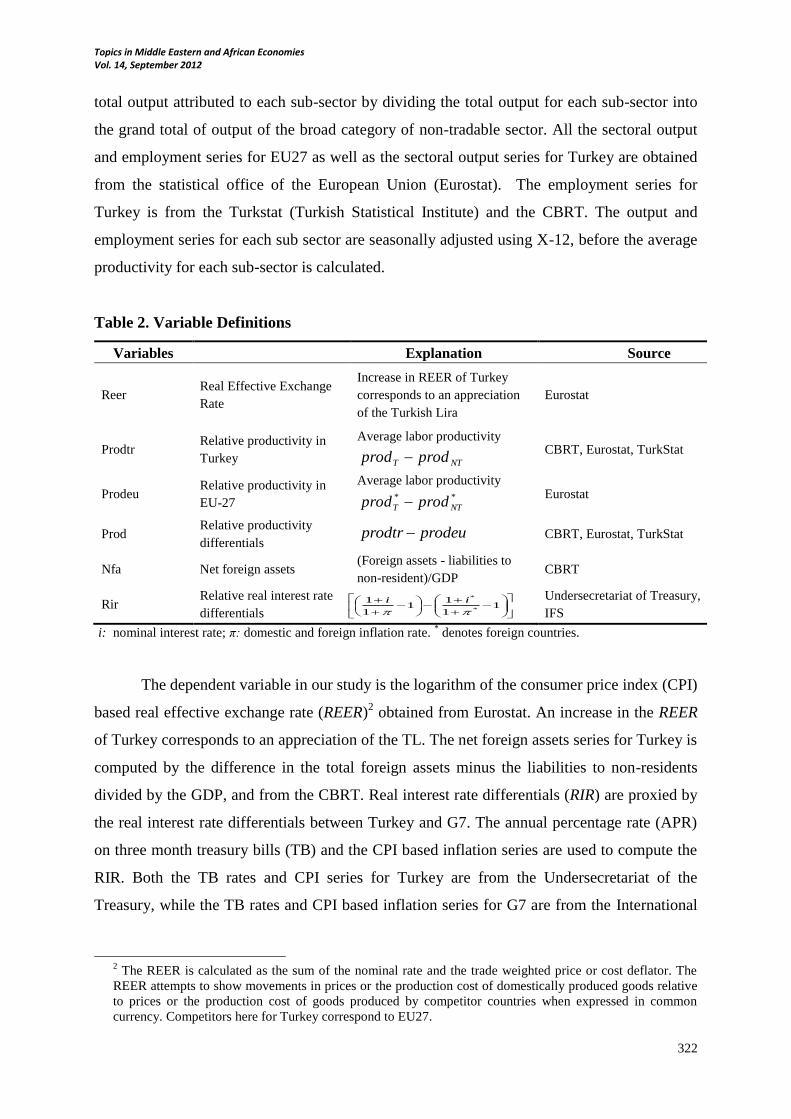
Table 2. Variable Definitions

Variables Explanation Source

Reer Real Effective Exchange

Rate

Increase in REER of Turkey

corresponds to an appreciation

of the Turkish Lira

Eurostat

Prodtr Relative productivity in

Turkey

Average labor productivity

NTT prodprod CBRT, Eurostat, TurkStat

Prodeu Relative productivity in

EU-27

Average labor productivity

**

NTT prodprod Eurostat

Prod Relative productivity

differentials prodeuprodtr CBRT, Eurostat, TurkStat

Nfa Net foreign assets (Foreign assets - liabilities to

non-resident)/GDP CBRT

Rir Relative real interest rate

differentials

Undersecretariat of Treasury,

IFS

i: nominal interest rate; π: domestic and foreign inflation rate. * denotes foreign countries.

The dependent variable in our study is the logarithm of the consumer price index (CPI)

based real effective exchange rate (REER)2 obtained from Eurostat. An increase in the REER

of Turkey corresponds to an appreciation of the TL. The net foreign assets series for Turkey is

computed by the difference in the total foreign assets minus the liabilities to non-residents

divided by the GDP, and from the CBRT. Real interest rate differentials (RIR) are proxied by

the real interest rate differentials between Turkey and G7. The annual percentage rate (APR)

on three month treasury bills (TB) and the CPI based inflation series are used to compute the

RIR. Both the TB rates and CPI series for Turkey are from the Undersecretariat of the

Treasury, while the TB rates and CPI based inflation series for G7 are from the International

2 The REER is calculated as the sum of the nominal rate and the trade weighted price or cost deflator. The

REER attempts to show movements in prices or the production cost of domestically produced goods relative

to prices or the production cost of goods produced by competitor countries when expressed in common

currency. Competitors here for Turkey correspond to EU27.

1

1

11

1

1*

*

ii


323

Financial Statistics (IFS). For Turkey the inflation series is calculated by the authors using the

Turkish CPI series. The variables used and the data sources are also summarized in Table 2.

Econometric Methodology

As a first step, we start by investigating the order of integration of the real exchange

rate and its determinants. Next, the stability of the relationship between the real exchange rate

and its determinants are assessed using the tests proposed by Kejriwal and Perron (2010)

involving non-stationary but cointegrated variables with multiple structural changes of

unknown timing in regression models. The global minimization procedure for the break

fractions is the same as in Bai and Perron (1998, 2003). It is obtained via an algorithm, using

the principle of dynamic-programming. Nevertheless, the distributions of the break fraction

estimates and the sub-Wald test statistics are different from the ones in Bai and Perron (1998,

2003) due to the nonstationarity of the time series. If the empirical application of the

Kejriwal-Perron tests corroborates the existence of structural break, then whether the

variables are indeed cointegrated needs to be verified, as these tests can reject the null of

stability when the regression is a spurious one (Kejriwal, 2008). So, the cointegration tests

following Kejriwal (2008), which are based on the extension of the one-break cointegration

tests developed by Aria and Kuruzomi (2007) (A-K henceforth) with a null of cointegration,

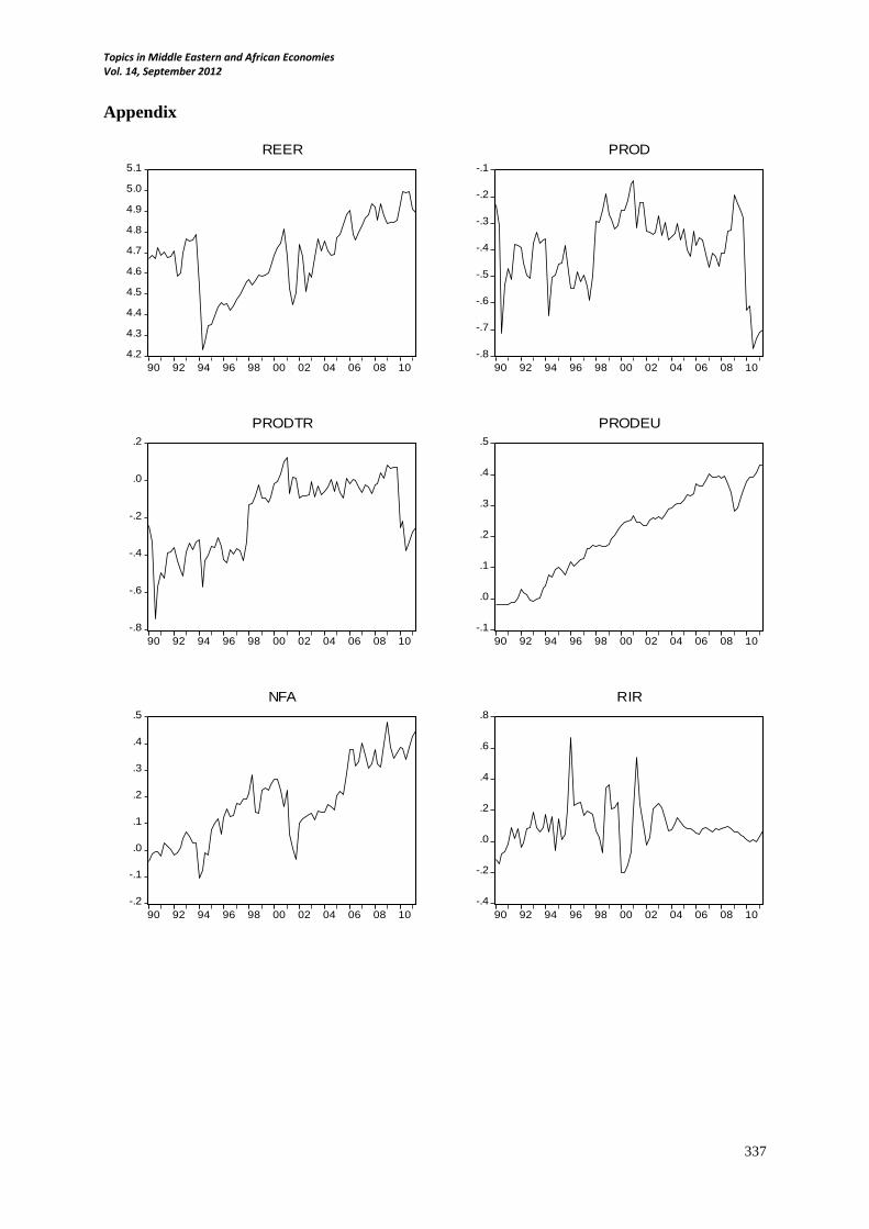
are performed. Because our series seem to exhibit a deterministic time trend (see the figures

in the Appendix), we include the trend in the unit root as well as cointegration tests. Finally,

we estimate the model with breaks to investigate how the relationship between the real

exchange rate and its determinants may have altered over time.

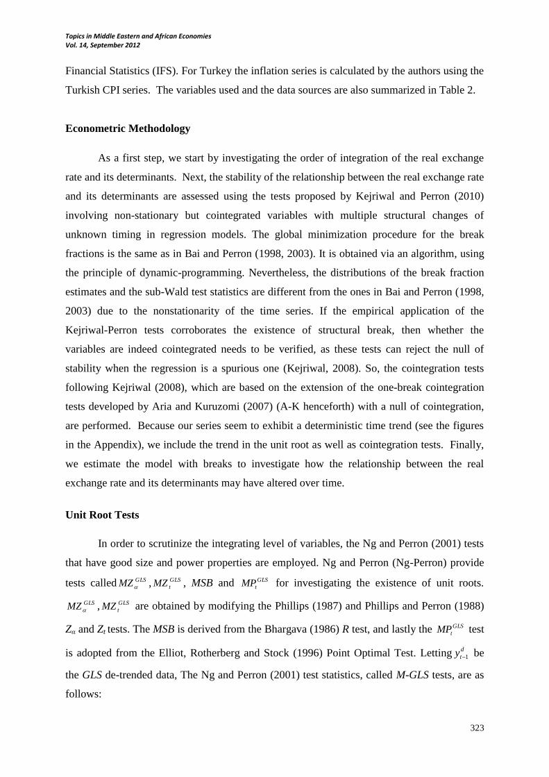
Unit Root Tests

In order to scrutinize the integrating level of variables, the Ng and Perron (2001) tests

that have good size and power properties are employed. Ng and Perron (Ng-Perron) provide

tests called GLSMZ , GLS

tMZ , MSB and GLS

tMP for investigating the existence of unit roots.

GLSMZ , GLS

tMZ are obtained by modifying the Phillips (1987) and Phillips and Perron (1988)

Zα and Zt tests. The MSB is derived from the Bhargava (1986) R test, and lastly the GLS

tMP test

is adopted from the Elliot, Rotherberg and Stock (1996) Point Optimal Test. Lettingd

ty 1 be

the GLS de-trended data, The Ng and Perron (2001) test statistics, called M-GLS tests, are as

follows:


324

)2/())(( 21 kfyTMZ d

T

d

a

MSBMZMZ a

d

t

2/1)/( fkMSBd

.,1/)()1(

1/(

0

212

0

212

txiffyTckc

xiffyTckcMP

t

d

T

t

d

Td

T

Where

T

t

d

t Tyk2

22

1 /)( ,

txif

xifc

t

t

,15.13

17 , and 0f is the frequency zero spectrum estimation.

In order to corroborate the results of the Ng-Perron tests, we also employ more

conventional unit root tests, namely ADF and KPSS tests.

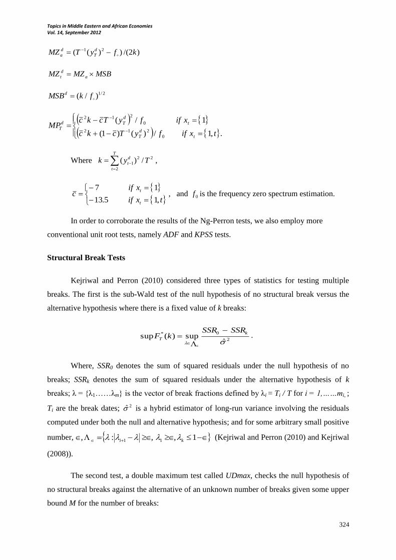
Structural Break Tests

Kejriwal and Perron (2010) considered three types of statistics for testing multiple

breaks. The first is the sub-Wald test of the null hypothesis of no structural break versus the

alternative hypothesis where there is a fixed value of k breaks:

2

0*

ˆsup)(sup

k

T

SSRSSRkF

.

Where, SSR0 denotes the sum of squared residuals under the null hypothesis of no

breaks; SSRk denotes the sum of squared residuals under the alternative hypothesis of k

breaks; λ = {λ1……λm} is the vector of break fractions defined by λi = Ti / T for i = 1,……mi, ;

Ti are the break dates; 2̂ is a hybrid estimator of long-run variance involving the residuals

computed under both the null and alternative hypothesis; and for some arbitrary small positive

number, 1,,:, 11 ki (Kejriwal and Perron (2010) and Kejriwal

(2008)).

The second test, a double maximum test called UDmax, checks the null hypothesis of

no structural breaks against the alternative of an unknown number of breaks given some upper

bound M for the number of breaks:


325

)(max)(max *

1

* kFMFUD Tmk

T

The third test involves a sequential procedure (SEQ) that analyzes the null hypothesis

of k breaks against the alternative hypothesis of k+1 breaks:

2

1

111

11 ˆ

ˆ,...,ˆ,,ˆ,...,ˆ()ˆ,....,ˆ(supmax)1(

, k

kjjTkT

kjT

TTTTSSRTTSSRkkSEQ

j

Where , 1 1 1ˆ ˆ ˆ ˆ ˆ ˆ: ( ) ( )j j j j j j jT T T T T T , and

2

1ˆ

k is a consistent

hybrid estimate of long run variance as in the SubF test given above. The model with k breaks

is obtained by a global minimization of the sum of squared residuals, as in Bai and Perron

(2003). The sequential procedure provides a consistent true number of breaks. However,

when the parameters change in such a way that the first and third regimes are identical, the

sequential procedure may end up selecting no breaks (Bai and Perron, 2006). A useful

strategy, then, to determine the number of breaks is to use SubF and UDmax tests which are

significant, and then use the sequential procedure to determine the number of breaks

(Kejriwal, 2008). As an alternative, the number of breaks can also be determined by using the

Bayesian information criterion (BIC) suggested by Yao (1998) and the modified Schwarz

criterion proposed by Liu et al. (1997) (LWZ), defined as;

,/)ln()(ˆln)( *2 TTpmmBIC and

.))(ln()/())/()ˆ,...,ˆ((ln)( 02

0

**

1

TcTppTTTSmLWZ mT

Where ).ˆ,....,ˆ()(ˆ,)1( 1

12*

mT TTSTmandpmqmp mTT ˆ,....,ˆ

1denote the

estimated break dates and )ˆ,....,ˆ( 1 mT TTS is the sum of squared residuals under m breaks. q is

the number of coefficients which are allowed to change and p is the number of coefficients

that are held fixed, and finally δ0 = 0.1 and c0 =0.299

In this study, stability tests for the relationship between the real effective exchange and

a number of regressors are performed, using the sequential procedure as well as the

information criteria, following Kejriwal (2008), to investigate the existence of breaks in the

real effective exchange rate regressions.


326

Cointegration Tests with Multiple Structural Breaks

Kejriwal and Perron (2010) show that the structural change tests they suggest have

good size and power properties. However, as pointed out in Kejriwal (2008) structural change

tests also have power against a purely spurious regression. This means that when the

cointegrating relation is unstable, the conventional cointegration tests are biased towards the

non-rejection of the null hypothesis of no cointegration Therefore, structural changes in the

cointegrating vector may be the reason for the findings of no cointegration in the literature.

Hence, cointegration analysis should consider the structural changes. Residual-based tests for

one structural change in the cointegration vector at an unknown time under the null of no

cointegration against several alternative hypotheses of cointegration are provided by Gregory

and Hansen (G-H) (1996). Nonetheless, these tests are developed to have power against the

alternative of a single break, and therefore can have a low power when there is more than a

single break in parameters Also, the test statistics, which are based on the minimal values of

overall possible breakpoints, are not in general consistent estimates of a break date if a change

exists (Kejriwal, 2008). Finally, if the primary concern is cointegration with structural breaks,

the null of cointegration is a more natural choice from the viewpoint of conventional

hypothesis testing.

To avoid these problems, Kejriwal (2008) extends the cointegration test with the

known or unknown one structural break tests proposed by A-K to analyze multiple structural

breaks under the null hypothesis of cointegration. In current study, following the work of A-K

and Kejriwal, we further augment the A-K model with a deterministic trend and allow shifts

in the trend as well. The regime and trend shift model used in this study is as follows:

Where k is the number of breaks, zt is a vector of I (1) regressors, given by

ztt uzz 1 , yt is the dependent I (1) variable, and by convention, T0=0 and Tk+1=T.

Augmenting the above regression model to deal with the simultaneity bias, we use the

dynamic OLS, adding the leads and lags of the first differences of the regressors.

1k1,..,ifor TtT ifuzztcy i-1i

*

t

l

lj

j

'

jti

'

tiit

T

T

The test statistic for k breaks, then, is given by:

11

1

22 )ˆ()ˆ(

~

T

t k

k

STV

.

111 k,..iforTtTifuztcy iiti

'

tiit


327

Where Ω11 is a consistent estimation of the long run variance of

kkt TTandTTTTu ˆ,....ˆ)/ˆ,......,/ˆ(ˆ, 11

* are obtained by minimizing the sum of the

squared residuals. The above test statistics are compared with the critical values provided by

A-K (2007) for one structural break. Critical values for multiple breaks are generated by the

authors, modifying the programs developed for Kejriwal (2008)3.

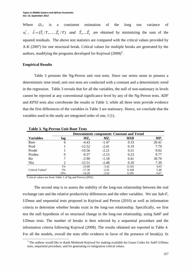
Empirical Results

Table 3 presents the Ng-Perron unit root tests. Since our series seem to possess a

deterministic time trend, unit root tests are conducted with a constant and a deterministic trend

in the regression. Table 3 reveals that for all the variables, the null of non-stationary in levels

cannot be rejected at any conventional significance level by any of the Ng-Perron tests. ADF

and KPSS tests also corroborate the results in Table 3, while all three tests provide evidence

that the first differences of the variables in Table 3 are stationary. Hence, we conclude that the

variables used in the study are integrated order of one, I (1).

aCritical values are from Table 1 of Ng and Perron (2001)

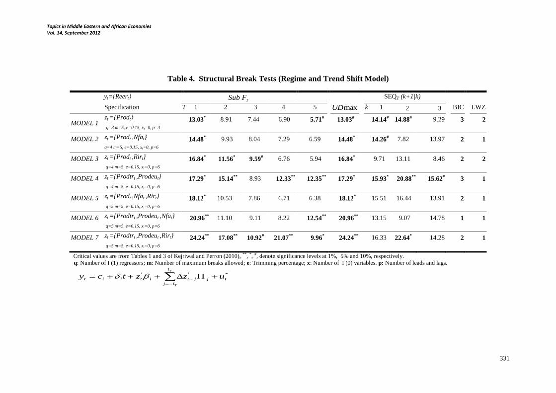
The second step is to assess the stability of the long-run relationship between the real

exchange rate and the relative productivity differences and the other variables. We use Sub-F,

UDmax and sequential tests proposed in Kejriwal and Perron (2010) as well as information

criteria to determine whether breaks exist in the long-run relationship. Specifically, we first

test the null hypothesis of no structural change in the long-run relationship, using SubF and

UDmax tests. The number of breaks is then selected by a sequential procedure and the

information criteria following Kejriwal (2008). The results obtained are reported in Table 4.

For all the models, overall the tests offer evidence in favor of the presence of break(s). In

3 The authors would like to thank Mohitosh Kejriwal for making available his Gauss Codes for SubF-UDmax

tests, sequential procedure, and for generating co-integration critical values.

Table 3. Ng-Perron Unit Root Tests

Deterministic component: Constant and Trend

Variables lag MZα MZt MSB MPt

Reer 6 -4.43 -1.47 0.33 20.41

Prod 1 -12.52 -2.41 0.19 7.79

Prodtr 1 -10.56 -2.21 0.21 9.02

Prodeu 0 -9.37 -2.15 0.23 9.77

Rir 7 -2.90 -1.18 0.41 30.70

Nfa 2 -12.51 -2.48 0.20 7.39

Critical Valuesa 1%

5%

10%

-23.80

-17.30

-14.20

-3.42

-2.91

-2.62

0.143

0.168

0.185

4.03

5.48

6.67


328

particular, at least one of the SubF, UDmax tests and the sequential procedure and both the

BIC and LWZ information criteria select at least one break for all the models studied. It is

important to point out that most break dates selected coincide with the period of two crises in

Turkey, in the mid-nineties and early 2000s. The mid-nineties and early 2000s were the

periods of financial and economic crises in Turkey, in which the Turkish lira lost its value

sharply, interest rates sky-rocketed, and inflation began to soar. The Turkish GDP was also

reduced significantly in these crises periods. The break fractions and the corresponding break

dates are reported in Tables 5 and 6, respectively. Table 6 clearly indicates that most of the

break points coincide with these crises periods.

The next step is to confirm the presence of cointegration among the real exchange rate

and the other variables to ensure that the rejection of stability is indeed derived from the

existence of a cointegration relationship with breaks, and not from a purely spurious

regression. In this context, first, both the conventional one break G-H, as well as A-K

cointegration tests, and second, cointegration tests with multiple breaks based on the A-K

framework, using the break dates selected by the sequential procedure and/or information

criteria, are performed.

Table 5 presents the results for G-H (1996) and A-K (2007) one structural break

cointegration tests in addition to the multiple structural break cointegration tests. For all the

tests, the regression representation is the regime and trend shift model, and the tests with

multiple breaks are based on the augmented version of the A-K framework. The results of the

G-H tests show we cannot reject the null of no cointegration for Models 1, 2, 3, and 5. For

Model 4, the null is rejected only by the ADFt test, and for Models 6 and 7 both by the Zt and

ADFt tests. The A-K one break test, on the other hand, rejects the null of cointegration at least

at the 5% significance level, except for Models 1 and 3. Putting it differently, A-K tests

cannot reject the null of cointegration at the 1% significance level, except for Model 5. In

short, G-H and A-K test results for one break are consistent at all conventional significance

levels only for Model 5, and certainly contradict each other for Models 1 and 3. The results

for the other models are mixed.

Turning to the two-break A-K tests, we cannot reject the null of cointegration for

Models 2 and 7 at any conventional significance level. The tests reject the null of

cointegration at 5% and 1% significance levels for Models 4, 5 and for Models 1, 3,

respectively. Finally, noting that we have evidence of three structural breaks only for Models


329

1 and 4, the A-K test, )ˆ(3

~

V , cannot reject the null of cointegration for Model 4, and rejects it

only at the 10% level for Model 1.

As the final step, we estimate the models for which there is evidence of cointegration,

and compare the coefficients for the sub periods to see how the cointegration relationship may

have changed over time. Table 6 shows estimated regressions with the regime and trend shift

model. Typically structural breaks are related to Turkey’s crises periods, such as 1994 and

2001. The estimated slope coefficients are denoted by φ1, φ2,…,φ9 in Table 6. As an example,

for Model 5, zt={prodt, Nfat, Rirt}, φ1-φ3, φ4-φ6 and φ7-φ9 show the estimated impact of prod,

Nfa and Rir on REER for regimes 1, 2, and 3 respectively. According to Table 6, for Models

1, 2, 3, and 7, relative productivity differentials are significant and have a positive sign, and

thereby are consistent with the B-S hypothesis before the structural break in 1994-1995.

However, after the 1994-95 structural-break through 2000s, relative productivities, as well as

the other explanatory variables, are not generally successful in explaining changes in the

REER.

The RIR either has the wrong sign or is not significant in all the models included. The

effect of NFA, on the other hand, is always positive and significant until 2001-2002. For

Model 2, it is significant until 2006, and for Model 6 for the whole sample period. The effect

of a 1% point increase in NFA appreciates the REER between 0.48% and 1.21%or about

0.8%, averaging over all the sub-periods. Overall, the results offer only very limited support

to the B-S hypothesis. In particular, the results do not support the productivity- REER

relationship for the post 2001 era, contrary to the emphasis placed on the B-S effect by the

CBRT. The only exception to this is the positive and significant coefficient for Prodtr in

Model 6. However, the magnitude of the Prodtr coefficient is small (0.17), and all the other

coefficients of Model 6 are either insignificant or have the wrong sign.

Conclusions

This paper analyzed the movements of the real effective exchange rate for the Turkish

economy for 1990:Q1-2011:Q2 using multiple structural breaks. According to the CBRT

Inflation Report II (2006), the experienced appreciation of the Turkish lira in recent years can

be attributed to relative productivity differentials. To explain movements of the real effective

exchange rate, seven models related to the B-S hypothesis are constituted by adding other

variables such as net foreign assets and real interest rate differentials.


330

According to the estimated cointegration relationships under multiple structural

breaks, the findings offer very limited support for the B-S hypothesis. The existence of the B-

S effect is generally limited to the pre-2001 period and in some cases even to the pre-1994

period. Given the span of our dataset and the econometric techniques employed, the results do

not support the emphasis placed on the B-S hypothesis by the CBRT.

Given the many determinants of the real exchange rate, the above results with a

limited number of variables and a relatively short span of data need to be interpreted with

caution. In particular, the liquidity surplus in the world in the 2000s combined with the

reduced risk premium for Turkey as a result of structural reforms and a relatively more stable

macroeconomic environment might have contributed to the wrong signs we obtained for the

real interest rate differentials. Furthermore, a change in the expectations about the future value

of the real exchange rate might be the driving force for the tendency of the Turkish lira to

appreciate in the 2000s. Future research needs to scrutinize these potential explanations as

well as the lack of support for the B-S hypothesis for Turkey in the 2000s.


331

Table 4. Structural Break Tests (Regime and Trend Shift Model)

yt={Reert} TFSub SEQT (k+1|k)

Specification T 1 2 3 4 5 maxUD k 1 2 3 BIC LWZ

MODEL 1 zt ={Prodt}

q=3 m=5, e=0.15, xt=0, p=3

13.03* 8.91

* 7.44

* 6.90 5.71

## 13.03

# 14.14

# 14.88

# 9.29 3 2

MODEL 2 zt ={Prodt ,Nfat}

q=4 m=5, e=0.15, xt=0, p=6

14.48* 9.93

** 8.04

* 7.29

* 6.59

* 14.48

* 14.26

# 7.82 13.97 2 1

MODEL 3 zt ={Prodt ,Rirt}

q=4 m=5, e=0.15, xt=0, p=6

16.84* 11.56

* 9.59

# 6.76

* 5.94

* 16.84

* 9.71 13.11

* 8.46 2 2

MODEL 4 zt ={Prodtrt ,Prodeut}

q=4 m=5, e=0.15, xt=0, p=6

17.29* 15.14

** 8.93* 12.33

** 12.35

** 17.29

* 15.93

* 20.88

** 15.62

# 3 1

MODEL 5 zt ={Prodt ,Nfat ,Rirt}

q=5 m=5, e=0.15, xt=0, p=6

18.12* 10.53

* 7.86

* 6.71

* 6.38

* 18.12

* 15.51

* 16.44

* 13.91 2 1

MODEL 6 zt ={Prodtrt ,Prodeut ,Nfat}

q=5 m=5, e=0.15, xt=0, p=6

20.96**

11.10 * 9.11

* 8.22

* 12.54

** 20.96

** 13.15

* 9.07

* 14.78 1 1

MODEL 7 zt ={Prodtrt ,Prodeut ,Rirt}

q=5 m=5, e=0.15, xt=0, p=6

24.24**

17.08**

10.92# 21.07

** 9.96

* 24.24

** 16.33

* 22.64

* 14.28 2 1

Critical values are from Tables 1 and 3 of Kejriwal and Perron (2010), **, *, #, denote significance levels at 1%, 5% and 10%, respectively.

q: Number of I (1) regressors; m: Number of maximum breaks allowed; e: Trimming percentage; x: Number of I (0) variables. p: Number of leads and lags.

*''

t

l

lj

jjtitiit uzztcyT

T


332

Table: 5. Gregory-Hansen and Arai-Kurozumi Cointegration Tests (Regime and Trend Shift Model)

G-H One Breakb A-K One Breaka A-K Two Breaksa A-K Three Breaksa

yt={Reert} *

tZ *

Z *

tADF )ˆ(1

~

V 1̂ )ˆ(2

~

V 1̂

2̂ )ˆ(3

~

V

1̂

2̂ 3̂

zt ={Prodt} Model 1 -3.83* -26.48 -4.22** 0.060 0.18 0.069** 0.18 0.52 0.023# 0.18 0.52 0.76

** %1

* %5

# %10

-6.02

-5.50

-5.24

-69.37

-58.58

-53.31

-6.02

-5.50

-5.24

0.118

0.085

0.069

0.052

0.037

0.032

0.031

0.024

0.021

zt ={Prodt , Nfat} Model 2 -4.31* -31.97 -4.42** 0.093* 0.18 0.029 0.18 0.76 - - - -

** %1

* %5

# %10

-6.45

-5.96

-5.72

-70.65

-68.43

-63.10

-6.45

-5.96

-5.72

0.100

0.068

0.057

0.055

0.037

0.031

zt ={Prodt , Rirt} Model 3 -4.38* -32.68 -4.46** 0.040 0.25 0.046** 0.18 0.52 - - - -

** %1

* %5

# %10

-6.45

-5.96

-5.72

-70.65

-68.43

-63.10

-6.45

-5.96

-5.72

0.088

0.061

0.049

0.044

0.032

0.027

zt ={Prodtrt , Prodeut} Model 4 -5.71* -49.19 -6.21* 0.080* 0.18 0.039* 0.18 0.52 0.018# 0.19 0.52 0.70

** %1

* %5

# %10

-6.45

-5.96

-5.72

-70.65

-68.43

-63.10

-6.45

-5.96

-5.72

0.100

0.068

0.057

0.044

0.032

0.027

0.027

0.020

0.018

zt ={Prodt , Nfat , Rirt} Model 5 -4.45* -33.82 -4.44** 0.115** 0.18 0.035* 0.18 0.55 - - - -

** %1

* %5

# %10

-6.89

-6.32

-6.16

-90.84

-78.87

-72.75

-6.89

-6.32

-6.16

0.083

0.055

0.045

0.035

0.026

0.022

zt ={Prodtrt , Prodeut ,Nfat} Model 6 -6.47* -60.03 -7.23** 0.057* 0.24 - - - - - - -

** %1

* %5

# %10

-6.89

-6.32

-6.16

-90.84

-78.87

-72.75

-6.89

-6.32

-6.16

0.074

0.052

0.042

zt ={Prodtrt , Prodeut , Rirt} Model 7 -6.45* -57.63 -6.37* 0.055* 0.21 0.026# 0.18 0.52 - - - -

** %1

* %5

# %10

-6.89

-6.32

-6.16

-90.84

-78.87

-72.75

-6.89

-6.32

-6.16

0.076

0.051

0.041

0.035

0.027

0.023 a Critical values are obtained by simulations using 100 steps and 2500 replications. **,*, #, denote significance levels at 1%, 5% and 10%, respectively. b Critical values are taken from Gregory-Hansen (1996)

*''

t

l

lj

jjtitiit uzztcyT

T


333

Table 6. Estimated Regressions with Multiple Structural Breaks (Regime and Trend Shift Model)

yt={Reert}

c1 c2 c3 c4 δ1 δ2 δ3 δ4 φ 1 φ 2 φ 3 φ 4 φ 5 φ 6 φ 7 φ 8

φ 9 1

T 2

T 3

T

zt ={Prodt}

BIC

SEQ

5.26 (0.00)

4.25 (0.00)

3.73 (0.00)

4.38 (0.00)

-0.02 (0.00)

0.01 (0.00)

0.01 (0.00)

0.01 (0.06)

0.97 (0.00)

0.23 (0.18)

-0.55 (0.21)

-0.14 (0.22) - - - - - 94:Q2 01:Q2 06:Q2

4.77 (0.00)

4.23 (0.00)

- - -0.00 (0.98)

0.01 (0.00)

- - 0.18 (0.59)

0.06 (0.42)

- - - - - - - 94:Q2 - -

zt ={Prodt , Nfat}

BIC SEQ

4.90 (0.00)

4.28 (0.00)

4.40 (0.00) -

-0.00 (0.55)

0.01 (0.00)

0.01 (0.02) -

0.42 (0.10)

0.24 (0.02)

-0.09 (0.32)

1.15 (0.01)

0.77 (0.00)

-0.17 (0.66) - - - 94:Q2 06:Q2 -

zt ={Prodt , Rirt}

5.51 (0.00)

4.39 (0.00) - -

-0.02 (0.00)

0.01 (0.00) - -

1.40 (0.00)

-0.00 (0.99)

-0.12 (0.64)

-0.45 (0.00) - - - - - 95:Q4 - -

zt ={Prodtrt , Prodeut}

SEQ

BIC

6.38 (0.00)

3.92 (0.00)

6.44 (0.00)

4.36 (0.00)

0.01 (0.49)

0.01 (0.03)

0.02 (0.00)

0.01 (0.00)

0.62 (0.14)

0.10 (0.56)

-0.88 (0.05)

-0.16 (0.29)

-2.12 (0.04)

0.05 (0.94)

-1.94 (0.16)

0.22 (0.47) - 94:Q2 01:Q2 05:Q1

LWZ

6.27 (0.00)

3.63 (0.00)

- - 0.01 (0.44)

0.01 (0.00)

- - 0.20 (0.70)

0.11 (0.22)

-1.77 (0.19)

0.50 (0.07)

-

- - - - 95:Q4 - -

zt ={Prodt , Nfat , Rirt}

BIC

4.79 (0.00)

4.18 (0.00)

4.44 (0.00) -

-0.00 (0.57)

0.01 (0.00)

0.01 (0.03) -

0.30 (0.17)

0.07 (0.60)

-0.08 (0.34)

1.21 (0.00)

0.76 (0.00)

0.19 (0.34)

-0.37 (0.16)

0.10 (0.18)

-0.65 (0.00) 94:Q2 02:Q1 -

zt ={Prodtrt , Prodeut ,Nfat}

BIC

LWZ 4.93 (0.00)

3.55 (0.00) - -

-0.00 (0.87)

0.00 (0.10) - -

0.40 (0.36)

0.17 (0.02)

-0.50 (0.71)

0.56 (0.01)

1.11 (0.04)

0.48 (0.00) - - - 94:Q2 - -

zt ={Prodtrt , Prodeut , Rirt}

LWZ

8.44 (0.00)

4.02 (0.00) - -

0.01 (0.33)

0.01 (0.00) - -

1.53 (0.00)

-0.01 (0.85)

-4.78 (0.00)

0.35 (0.12)

-0.51 (0.05)

-0.34 (0.00) - - - 94:Q2 - -

BIC

6.56 (0.00)

4.12 (0.00)

3.77 (0.00)

- 0.01 (0.22)

0.02 (0.05)

0.01 (0.00)

- 0.74 (0.06)

0.02 (0.92)

0.02 (0.88)

-2.41 (0.03)

-0.13 (0.88)

0.47 (0.03)

-0.37 (0.20)

-0.05 (0.64)

-0.45 (0.00)

94:Q2 01:Q2 -

p-values are in parenthesis. *''

t

l

lj

jjtitiit uzztcyT

T


334

References

Alberola, E., and D. Naiva. “Equilibrium Exchange Rates in the New EU Members: External

Imbalances vs. Real Convergence.” Review of Development Economics, 12(3), 2008,

605-619.

Alberola, E., S. G. Cervero, H. López, and A. Ubide. “Global Equilibrium Exchange Rates:

Euro, Dollar, “Ins”, “Outs” and Other Major Currencies in a Panel Cointegration

Framework.” IMF Working Paper, 99 (175), 1999.

Alper, A. M., and I. Civcir. “Can Overvaluation Prelude to crisis and Harm Growth in

Turkey.” Journal of Policing Modeling, 34 (1), 2012, 112-131.

Arai, Y., and E. Kurozumi. “Testing for the Null Hypothesis of Cointegration with a

Structural Break,” Econometric Reviews, 26 (6), 2007, 705-739.

Bai, J., and P. Perron. “Estimating and Testing Linear Models with Multiple Structural

Changes,” Econometrica, 66, 1998, 47-78.

Bai, J., and P. Perron. “Computation and Analysis of Multiple Structural Change Models,”

Journal of Applied Econometrics, 18, 2003, 1-22.

Bai, J., and P. Perron. “Multiple Structural Change Models: A Simulation Analysis,” in D.

Corbea, S.Durlauf and B.E. Hansen (eds), Econometric Theory Practice Frontiers of

Analysis Applied Research, Cambridge University Press, 2006, 212-237.

Balassa, Bela. “Purchasing Power Parity Doctrine: A Reappraisal,” The Journal of Political

Economy, 72, 1964, 584-596.

Bénassy-Quéré, A., S. Béreau, and V. Mignon. “On the Complementarity of Equilibrium

Exchange-Rate Approaches, Review of International Economics, 18 (4), 2010, 618–632.

Bhagwati, Jagdish, N. “Why are Services Cheaper in Poor Countries?” Economic Journal, 94

(374), 1984, 279–286.

Bhargava, A. ,“On the Theory of Testing for Unit Roots in Observed Time Series,” Review of

Economic Studies, 53 (3), 1986, 369-384.

Camarero, Mariam. “The Real Exchange Rate of the Dollar for a Panel of OECD Countries:

Balassa-Samuelson or Distribution Sector Effect,” Journal of Comparative Economics,

36, 2008, 620-632.

Clark, P. B., and R. MacDonald. “Filtering the BEER: A Permanent and Transitory

Decomposition.” IMF Working Paper, 00 (144), 2000.

Coudert, V., and C. Couharde. “Currency Misalignments and Exchange Rate Regimes in

Emerging and Developing Countries.” Review of International Economics, 17(1),

2009, 121-136.


335

Égert, Balasz. “Balassa-Samuelson Meets South Eastern Europe, the CIS and Turkey: A

Close Encounter of the Third Kind?,” European Journal of Comparative Economics, 2

(2), 2005, 221-243

Égert, B., L. Halpern, and R. MacDonald. “Equilibrium Exchange Rates in Transition

Economies: Taking Stock of the Issues,” Journal of Economic Surveys, 20 (2), 2006,

257-324.

Elliot, G., T. J. Rothenberg, and J. Stock. “Efficient Test for an Autoregressive Unit Root,”

Econometrica, 64, 1996, 813-36.

Gente, Karine. “The Balassa-Samuelson Effect in a Developing Country,” Review of

Development Economics, 10 (4), 2006, 683-699.

Gregory, A. W. and B.E. Hansen. “Tests for the Cointegration in Models with Regime and

Trend Shifts,” Oxford Bulletin of Economics and Statistics, 58 (3), 1996, 555-560.

Inflation Report II (2006), Inflation Report, The Central Bank of the Republic of Turkey

http://www.tcmb.gov.tr/yeni/eng/ (12/25/2011).

Kanamori, T. and Z. Zhao. The Renminbi Exchange Rate Revaluation: Theory, Practice and

Lessons from Japan, Asian Development Bank Institute, 2006,

http://www.adbi.org/files/2006.05.09.book.renminbi.exchange.rate.pdf (10/20/2011).

Kejriwal, M. and Perron, P., “Testing for Multiple Structural Changes in Cointegrated

Regression Models,” American Statistical Association Journal of Business and

Economic Statics, 28 (4), 2010, 503-522.

Kejriwal, M., “Cointegration with Structural Breaks: An Application to the Feldstein-Horioka

Puzzle,” Studies in Nonlinear Dynamics and Econometrics, 12 (1), 2008, Article 3.

Kravis, I. B., and R. E. Lipsey. “Toward an Explanation of National Price Levels”, NBER

Working Paper Series, 1034, 1982, 1-52.

Lane, P., R., and M. G. Milesi-Feretti. “The Transfer Problem Revisited: Net Foreign Assets

and Real Exchange Rates,” The Review of Economics and Statistics, 86 (4), 2004, 841-

857.

Liu, J., Wu, S. and J. V. Zidek. “On Segmented Multivariate Regression,” Statistica Sinica, 7,

1997, 497-525.

Lommatzsch, K., and S. Tober. “What is behind the Real Appreciation of the Accession

Countries’ Currencies? An Investigation of the PPI-based Real Exchange Rate,”

Economic Systems, 28 (4), 2004.,383–403.

http://www.tcmb.gov.tr/yeni/eng/

http://www.adbi.org/files/2006.05.09.book.renminbi.exchange.rate.pdf


336

MacDonald, R., and J. Nagayasu. “The Long-Run Relationship between Real Exchange Rates

and Real Interest Rate Differentials: A Panel Study.” IMF Staff Papers, 47(1) ,2000,

116-128.

MacDonald, R., and L. Ricci, “Estimation of the Equilibrium Real Exchange Rate for South

Africa,” IMF Working Paper, 3 (44), 2003.

MacDonald, R., and L. Ricci. “The Real Exchange Rate and the Balassa Samuelson Effect:

The Role of the Distribution Sector,” Pacific Economic Review, 10, no.1, 2005, 29-48.

MacDonald, R., and C. Wojcik. “Catching up: The Role of Demand, Supply and Regulated

Price Effects on the Real Exchange Rates of Four Accession Countries,” Economics of

Transition, 12 (1), 2004, 153–179.

Mejean, Isabelle, “Can Firms Location Decisions Counteract the Balassa Samuelson Effect?”

Journal of International Economics, 76, 2008, 139-154.

Ng, S., and P. Perron. “Lag Length Selection and the Construction of Unit Root Tests with

Good Size and Power,” Econometrica, 69, 2001, 1519-1554.

Obstfeld, M., and K. Rogoff., Foundations of International Macroeconomics, Cambridge,

MA: The MIT Press, 1996.

Phillips, P.C.B. “Times Series Regression with a Unit Root,” Econometrica, 55, 1987, 277-

301.

Phillips, P.C.B., and P. Perron. “Testing for a Unit Root in Time Series Regression,”

Biometrika, 75, 1988, 335-346.

Rahn, Jörg. “Bilateral Equilibrium Exchange Rates of EU Accession Countries Against the

Euro.” BOFIT Discussion Paper, 11, 2003. 1-29

Samuelson, Pau, A., “Theoretical Notes on Trade Problems,” Review of Economics and

Statistics, 46 (2), 1964, 145-54.

Yao, Y., C. “Estimating the Number of Change Points via Schwartz Criterion”, Statistics and

Probability Letters, 6, 1988, 181-189


337

Appendix

4.2

4.3

4.4

4.5

4.6

4.7

4.8

4.9

5.0

5.1

90 92 94 96 98 00 02 04 06 08 10

REER

-.8

-.7

-.6

-.5

-.4

-.3

-.2

-.1

90 92 94 96 98 00 02 04 06 08 10

PROD

-.8

-.6

-.4

-.2

.0

.2

90 92 94 96 98 00 02 04 06 08 10

PRODTR

-.1

.0

.1

.2

.3

.4

.5

90 92 94 96 98 00 02 04 06 08 10

PRODEU

-.2

-.1

.0

.1

.2

.3

.4

.5

90 92 94 96 98 00 02 04 06 08 10

NFA

-.4

-.2

.0

.2

.4

.6

.8

90 92 94 96 98 00 02 04 06 08 10

RIR

Documents

Can Productivity Increases Really Explain The Lira