Can Land Broadband Seismic Be as Good as Marine Broadband

O f f s h o r e a n d o n s h o r e b r o a d b a n d s e i s m o l o g y

1382 The Leading Edge November 2013

SPECIAL SECTION: Offshore and onshore broadband seismology

Can land broadband seismic be as good as marine broadband?

The recent development of techniques to extend the bandwidth of marine towed-streamer surveys has

significantly changed the marine seismic landscape. In fact, it has coined the new category of “broadband seismic,” now synonymous with the marine towed-streamer market.

The bandwidth challenge for marine towed-streamer seismic is well documented and is related to mitigating, or completely removing, the interference pattern from the inter-action of the upgoing primary wave and its surface reflection (i.e., its ghost) at the source and receiver side. The interfer-ence results in the ghost notches in the amplitude spectrum which bound the useful bandwidth of the data at the high and low ends of the spectrum.

Over the last few years, we have seen the proliferation of broadband solutions (which employ specific combinations of equipment, acquisition techniques, and processing meth-odologies) as well as standalone broadband processing treat-ments which can be applied in a variety of situations. The best broadband results to date have come from the solutions which have tackled both the receiver and source ghost notch-es to extend the seismic bandwidth to more than six octaves.

Broadband benefitsBefore we consider whether we can achieve similar results with onshore surveys, let us try to qualitatively define the characteristics and benefits of six-octave bandwidth seismic that constitute our current benchmark. We will use data examples from a 3D narrow-azimuth survey using variable-depth streamer acquisition (Soubaras, 2010) in the Santos

MICHEL DENIS, VALÉRIE BREM, FABIENNE PRADALIE, FREDERIC MOINET, MATTHIEU RETAILLEAU, JEREMY LANGLOIS, BING BAI, and ROGER TAYLOR, CGGVAUGHAN CHAMBERLAIN and IAN FRITH, AngloGold Ashanti

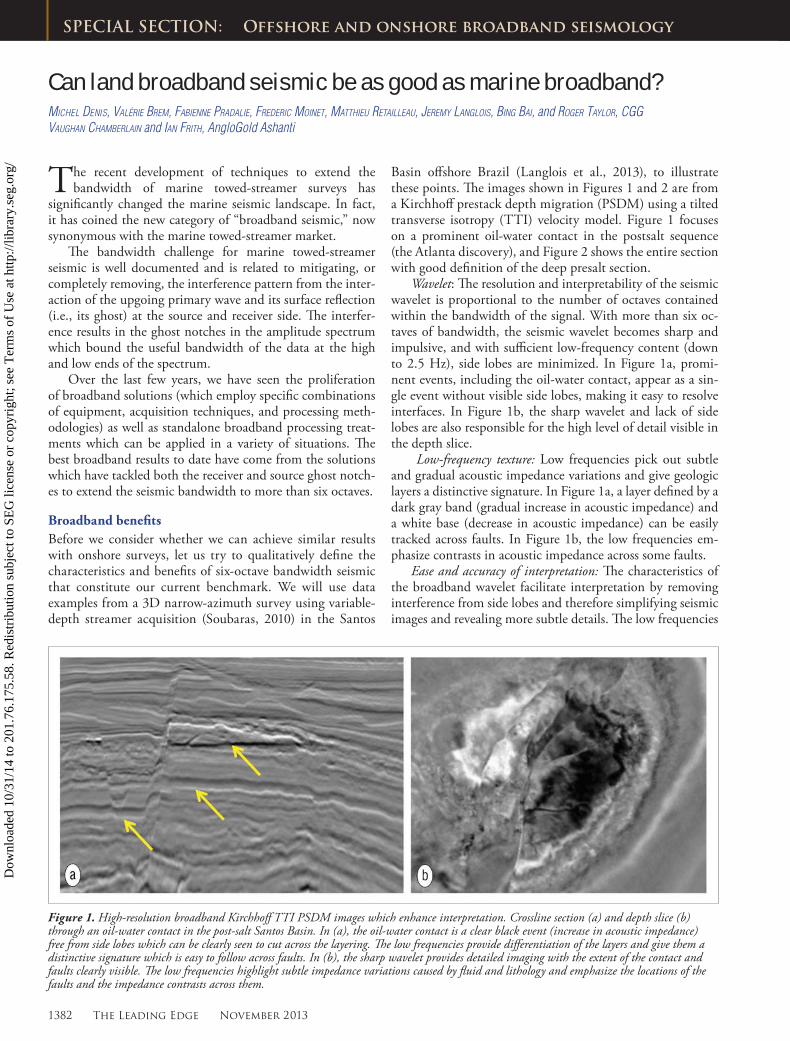
Basin offshore Brazil (Langlois et al., 2013), to illustrate these points. The images shown in Figures 1 and 2 are from a Kirchhoff prestack depth migration (PSDM) using a tilted transverse isotropy (TTI) velocity model. Figure 1 focuses on a prominent oil-water contact in the postsalt sequence (the Atlanta discovery), and Figure 2 shows the entire section with good definition of the deep presalt section.

Wavelet: The resolution and interpretability of the seismic wavelet is proportional to the number of octaves contained within the bandwidth of the signal. With more than six oc-taves of bandwidth, the seismic wavelet becomes sharp and impulsive, and with sufficient low-frequency content (down to 2.5 Hz), side lobes are minimized. In Figure 1a, promi-nent events, including the oil-water contact, appear as a sin-gle event without visible side lobes, making it easy to resolve interfaces. In Figure 1b, the sharp wavelet and lack of side lobes are also responsible for the high level of detail visible in the depth slice.

Low-frequency texture: Low frequencies pick out subtle and gradual acoustic impedance variations and give geologic layers a distinctive signature. In Figure 1a, a layer defined by a dark gray band (gradual increase in acoustic impedance) and a white base (decrease in acoustic impedance) can be easily tracked across faults. In Figure 1b, the low frequencies em-phasize contrasts in acoustic impedance across some faults.

Ease and accuracy of interpretation: The characteristics of the broadband wavelet facilitate interpretation by removing interference from side lobes and therefore simplifying seismic images and revealing more subtle details. The low frequencies

Figure 1. High-resolution broadband Kirchhoff TTI PSDM images which enhance interpretation. Crossline section (a) and depth slice (b) through an oil-water contact in the post-salt Santos Basin. In (a), the oil-water contact is a clear black event (increase in acoustic impedance) free from side lobes which can be clearly seen to cut across the layering. The low frequencies provide differentiation of the layers and give them a distinctive signature which is easy to follow across faults. In (b), the sharp wavelet provides detailed imaging with the extent of the contact and faults clearly visible. The low frequencies highlight subtle impedance variations caused by fluid and lithology and emphasize the locations of the faults and the impedance contrasts across them.

Dow

nloa

ded

10/3

1/14

to 2

01.7

6.17

5.58

. Red

istr

ibut

ion

subj

ect t

o SE

G li

cens

e or

cop

yrig

ht; s

ee T

erm

s of

Use

at h

ttp://

libra

ry.s

eg.o

rg/

November 2013 The Leading Edge 1383


successfully preserve bandwidth during data processing. In the case of the vibroseis source, bandwidth can also be limited by our ability to generate sufficient low- and high-frequency energy that can penetrate the near-surface. Although recent work has been done to investigate the onshore ghost effect, the case studies in this article do not cover this issue.

To summarize, matching the benchmark set by the recent marine towed-streamer broadband techniques is not a trivial exercise in the onshore environment.

Benefits of high-density acquisition onshoreAn increasing body of evidence in the industry points to the improvements in seismic imaging that can be achieved by

highlight subtle impedance variations caused by fluid and lithology and clearly show the faulted reservoir compartments in Figure 1b. Duval (2012) demonstrates that broadband data are less subject to tuning effects and allow interpreta-tion of pinch-outs and thin beds which cannot be resolved by conventional band-limited seismic. In addition, automated horizon picking has been shown to be quicker (more data-driven with fewer manual interventions) and more accurate, and horizon amplitude extractions are cleaner and less noisy.

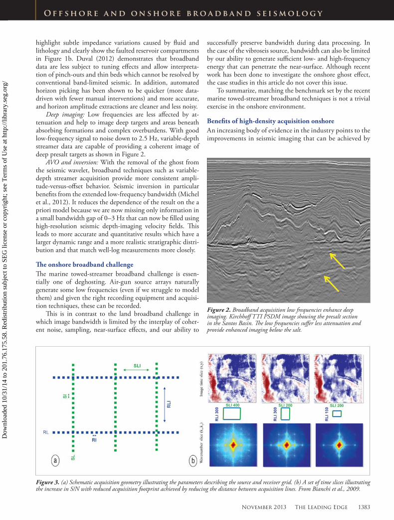
Deep imaging: Low frequencies are less affected by at-tenuation and help to image deep targets and areas beneath absorbing formations and complex overburdens. With good low-frequency signal to noise down to 2.5 Hz, variable-depth streamer data are capable of providing a coherent image of deep presalt targets as shown in Figure 2.

AVO and inversion: With the removal of the ghost from the seismic wavelet, broadband techniques such as variable-depth streamer acquisition provide more consistent ampli-tude-versus-offset behavior. Seismic inversion in particular benefits from the extended low-frequency bandwidth (Michel et al., 2012). It reduces the dependence of the result on the a priori model because we are now missing only information in a small bandwidth gap of 0–3 Hz that can now be filled using high-resolution seismic depth-imaging velocity fields. This leads to more accurate and quantitative results which have a larger dynamic range and a more realistic stratigraphic distri-bution and that match well-log measurements more closely.

The onshore broadband challengeThe marine towed-streamer broadband challenge is essen-tially one of deghosting. Air-gun source arrays naturally generate some low frequencies (even if we struggle to model them) and given the right recording equipment and acquisi-tion techniques, these can be recorded.

This is in contrast to the land broadband challenge in which image bandwidth is limited by the interplay of coher-ent noise, sampling, near-surface effects, and our ability to

Figure 2. Broadband acquisition low frequencies enhance deep imaging. Kirchhoff TTI PSDM image showing the presalt section in the Santos Basin. The low frequencies suffer less attenuation and provide enhanced imaging below the salt.

Figure 3. (a) Schematic acquisition geometry illustrating the parameters describing the source and receiver grid. (b) A set of time slices illustrating the increase in S/N with reduced acquisition footprint achieved by reducing the distance between acquisition lines. From Bianchi et al., 2009.

Dow

nloa

ded

10/3

1/14

to 2

01.7

6.17

5.58

. Red

istr

ibut

ion

subj

ect t

o SE

G li

cens

e or

cop

yrig

ht; s

ee T

erm

s of

Use

at h

ttp://

libra

ry.s

eg.o

rg/



increasing source and receiver density, with examples avail-able in a range of geologic settings from the North Slope of Alaska (Firth et al., 2012) to the Middle East (Seeni et al., 2011). For the acquisition geometry, the parameters, in or-der of importance, are: source and receiver line increments (SLI, RLI), source and receiver station intervals along ac-quisition lines (SI, RI), and source and receiver array size.

By decreasing the distance between source and receiver lines, aliasing in the stack response is reduced (Bianchi et al., 2009). This has a major impact on the signal-to-noise ratio with better noise cancellation, reduced acquisition imprint (Figure 3), and additional benefits for imaging. For wide-azi-muth common-offset vector (COV) imaging schemes, offset vector sampling distances are reduced for higher-resolution imaging and more accurate orthorhombic velocity analysis leading to improving signal summation. Reduced SLI and RLI distances also allow us to record short offsets to improve inversion for near-surface velocities which will improve the imaging of shallow and deep targets.

Moving from the line spacing to source and receiver intervals, by de-creasing the distance between source (SI) and receiver stations (RI), we can better sample the slow-velocity surface wave. Because it is difficult to fully remove aliased coherent noise in a way that preserves the amplitude of the primaries, sufficient sampling of slow-velocity arrivals helps us to re-move these waves and preserve the signal over a large range of frequen-cies. Reduced bin size based on the smaller SI and RI values also im-proves imaging resolution by remov-ing the need for frequency filtering when migrating the data. This means that a small RI and SI value is a re-quirement to maximize the benefits of broadband sources (on the high-frequency side) by delivering optimal vertical and lateral resolution.

The final consideration in our schematic geometry is the array size. The reduction of the SLI, RLI, SI, and RI parameters naturally leads to a reduction of field array size on both source and receiver sides. This has two major benefits.

The first benefit relates to opera-tional efficiency during acquisition; small arrays imply narrower acquisi-tion lines and a reduced amount of line opening work. Reduction in the size of receiver arrays also implies fewer sensors to deploy, transport,

and maintain. For vibroseis operations, reduced source arrays increase source fleet efficiency and maneuverability. Despite early concerns in reducing the number of vibrators per fleet (and therefore the energy emitted per shotpoint), Bianchi et al. (2009) demonstrate that this is more than compensated by the increase in shotpoint density and the associated benefits discussed earlier.

When arrays are reduced to a single element, we end up with single-source, single-receiver acquisition which brings further acquisition efficiencies. On the subsurface imaging side, we observe that high-density, long-offset, wide-azimuth surveys recorded with single source and single receivers pro-vide a notably high signal-to-noise ratio and fine resolution from very shallow to deep across all reservoir levels (Seeni et al., 2011). The use of dense single source and single receivers yields the following benefits:

Figure 4. Sampling and attenuation of slow-velocity surface waves on common source gathers (x, t) as a function of array size: (a) single sensor, (b) 2 × 2 array, and (c) 4 × 4 array. Corresponding (f, k) displays are shown as a function of receiver station interval: (d) RI, (e) 2 × RI, and (f ) 4 × RI. Although the surface-wave amplitude is reduced by the field array, it can be seen that the remaining energy is progressively more aliased as array size increases.

Dow

nloa

ded

10/3

1/14

to 2

01.7

6.17

5.58

. Red

istr

ibut

ion

subj

ect t

o SE

G li

cens

e or

cop

yrig

ht; s

ee T

erm

s of

Use

at h

ttp://

libra

ry.s

eg.o

rg/



• higher productivity with more efficient equipment use and independent single vibrators

• more accurate azimuthal measurements (no directivity bias from field arrays)

• improved coherent noise attenuation with properly sampled low-velocity waves

• improved near-surface model and surface-consistent pro-cessing with denser sampling (statics, deconvolution, etc.)

• high imaging signal-to-noise ratio and exceptional spatial and temporal bandwidths with small bin sizes and mini-mal acquisition footprint

• optimal imaging at all target depths

Field arrays are still popular, and their main purpose is to at-tenuate surface waves. The sampling interval within the arrays is small enough to properly sample slow-velocity waves, but the finite length of the array and the simple analog summation in-volved makes them poor performers compared to digital low-pass filters. As a result, slow-velocity waves are only slightly attenuated, with remaining amplitude levels still much higher than the signal and often aliased (Figure 4) because of to the large distances between stations. A more effective solution is to use smaller arrays or single source/receivers with a small SI and RI. In this way, the surface waves are well sampled and easy to remove at the processing stage without damaging underlying primaries. In fact, the real issue is aliased sampling and not high-amplitude surface waves. To summarize, field arrays have limited noise reduction capabilities; they introduce directivity bias and intra-array distortions.

Broadband sourcesAs discussed earlier, low frequencies benefit a range of applica-tions from improved seismic interpretation in general to deep imaging and more quantitative inversion results. Our preferred onshore source is vibroseis, particularly for high-productivity operations on dense source grids. A range of solutions for broadband vibroseis sweeps has been developed and can be customized and deployed for all types of objectives (Meunier and Bianchi, 2012). There has been a particular focus on low-dwell, nonlinear sweeps (Baeten et al., 2010) to increase vibra-tor output at low frequencies, which has led to sweeps start-ing as low as 1.5 Hz being used in production. To put this in context, recent examples suggest that we are now able to input lower frequencies with vibroseis than with marine air guns or, in fact, conventional dynamite shots onshore.

Broadband receiversThere is an ongoing discussion as to the best choice from the current range of commercially available receiver technology to record an extended bandwidth. One important aspect is the performance of the industry-standard 10-Hz analog geophones versus the current generation of digital sensors for recording low frequencies, discussed in detail by Maxwell et al. (2011).

MEMS (micromachined electromechanical systems) digital accelerometers have a lesser roll-off to low frequencies (–6 dB instead of –12 dB in the velocity domain compared to analog geophones). In addition, they have a response to DC, which

should make them good candidates for low-frequency record-ing. However, the noise floor of these digital sensors, which is higher than that of an analog geophone system, may be a limitation for recording low-amplitude, low-frequency signals.

Another class of electronically controlled sensor is based on geophones which have amplitude responses that are flattened around their resonant frequency to create a roll-off to low frequencies which is not as sharp as analog geophones.

Contrary to popular perception, industry-standard 10-Hz analog geophones can be a valid option for low-frequency recording. Maxwell et al. (2011) state that a 10-Hz geophone (with 70% damping) is already –3 dB at 10 Hz and will be an additional –24 dB at 2.5 Hz. However, because the geophone low-frequency roll-off is a mechanical effect, it will reduce the signal and ambient noise by the same degree, preserving the signal-to-(ambient) noise ratio. Maxwell et al. (2011) con-clude that with reasonable signal strength (relative to instru-ment noise), we can typically flatten the geophone response to about two octaves below the natural frequency; so for a 10-Hz geophone, we can get down to about 2.5 Hz.

Finally, a new generation of high-sensitivity geophones is now available with a natural frequency of 5 Hz. These are specifically designed for single-sensor application and provide excellent low-frequency recording.

Both of our case studies, by coincidence, feature data re-corded with 10-Hz analog geophones. This does not reflect any bias on behalf of the authors for or against digital sen-sors or analog geophones. However, the second case study is a good demonstration of our ability to recover frequencies down to the 2– 4-Hz octave from analog geophones.

Case study 1: Broadband land seismic for mining applicationsOur first case study comes from South Africa (Denis et al., 2013). To evaluate the value of dense broadband seismic for the mining industry, AngloGold Ashanti (AGA) commis-sioned a test survey over a prospect area of 35 km2 located 160 km southwest of Johannesburg. The geologic objectives of this test were to image the formations above the Vaal Reef (a gold-bearing conglomerate in the Witwatersrand Basin) and define the features that bound and modify the Vaal Reef target blocks at depths ranging from 2.7 to 3.8 km. This test was an opportunity to illustrate how new onshore acquisition techniques, dense geometries, and the latest pro-cessing can improve land seismic imaging.

The survey was acquired on a fixed spread (Figure 5) and processed as a fast track on site. Figure 6 compares the legacy conventional data set acquired in 1996 and the new high-den-sity broadband data set. To explore the specific contribution of the increased bandwidth, the broadband data set is also shown filtered to the bandwidth of the legacy survey (Figure 6b):

1) Legacy data set: SLI 420 m, SI 70 m, RLI 300 m, RI 50 m; 10-90 Hz sweep

2) Dense acquisition: SLI 50 m, SI 50 m, RLI 100 m, RI 50 m; filtered to 10–90 Hz

Dow

nloa

ded

10/3

1/14

to 2

01.7

6.17

5.58

. Red

istr

ibut

ion

subj

ect t

o SE

G li

cens

e or

cop

yrig

ht; s

ee T

erm

s of

Use

at h

ttp://

libra

ry.s

eg.o

rg/



3) Dense broadband acquisition: SLI 50 m, SI 50 m, RLI 100 m, RI 50 m; 3–160 Hz sweep

Our expectations from the dense acquisition are met and the poststack time migration (post-STM) image quality is out-standing at all depths, from ultrashallow to deep targets, as seen in Figure 6. With this level of image quality, it was pos-sible to significantly improve the velocity model to give opti-mal focusing and positioning of the seismic reflections with a prestack time migration final product. The broadband vibro-seis sweep achieves remarkable seismic wavelet compression with a sharp main lobe and minimum side lobes, thanks to the addition of nearly one octave at the high end and close to two octaves at the low end of the spectrum. With a band-width just short of six octaves, the images have a broadband texture with greatly improved stratigraphic and structural detail available for interpretation.

Case study 2: Broadband land seismic in the Middle EastOnshore North Africa and the Middle East have been at the forefront of land seismic technology in recent years. These re-gions typically offer open terrain where large seismic spreads can be deployed and vibrators have good access, making it ideal for the deployment of high-channel-count crews and high-productivity vibroseis operations for high-density wide-azimuth surveys.

The survey in this case study was acquired in 2010 and covered 2600 km2 in an exploration area with sparse well cov-erage. A dense 50 50-m shotpoint grid was acquired with single vibrators operating using the distance separated simul-taneous sweeping technique (Bouska, 2009). The receiver line spacing was 250 m with 25-m inline spacing of arrays of 12 geophones. The survey geometry provided maximum inline offsets of 8 km, crossline offsets of 6.5 km, and a nominal fold of 8320 for 25- 25-m bins. The survey started with a conventional vibroseis sweep of 6–86 Hz, but this was replaced by a 1.5–86 Hz broadband sweep partway through the survey after successful testing.

Initial processing using a con-ventional sequence produced results that were somewhat disappointing because the extended low-frequency bandwidth was not evident in the fi-nal migrated images. This resulted in reprocessing tests to try to recover the full bandwidth of the data.

For the initial reprocessing tests on this data set, recovery of the low-frequency signal was accom-plished initially through geophone amplitude compensation down to 2

Hz applied to the shot gathers, followed by poststack am-plitude balancing on octave slices derived from a frequency decomposition of the stack. The geophone amplitude com-pensation resulted in noise being boosted on the individual traces, but after pre-STM on this high-density data set, a good level of signal to noise was achieved. The poststack amplitude balancing of the octave slices from frequency decomposition was done using long windows (2000 ms) to ensure that the relative amplitude of reflectors was preserved and the geologic character was not changed. This further boosted the low-fre-quency signal but did not result in any significant increase in the noise, except in the octaves below 2 Hz where the signal-to-noise ratio was marginal or poor, as shown in Figure 7.

Figure 5. Case study 1. Acquisition geometry with nominal source positions shown in red and the nominal fixed receiver spread shown in blue.

Figure 6. Case study 1. Comparison of post-STM images for (a) legacy conventional data set, 10–90 Hz: (b) high-density data set filtered to conventional bandwidth, 10–90 Hz; and (c) full-bandwidth high-density data set, 3–160 Hz. With nearly six octaves of bandwidth, the quality of (c) approaches our marine broadband benchmark. Data courtesy of AngloGold Ashanti.

Dow

nloa

ded

10/3

1/14

to 2

01.7

6.17

5.58

. Red

istr

ibut

ion

subj

ect t

o SE

G li

cens

e or

cop

yrig

ht; s

ee T

erm

s of

Use

at h

ttp://

libra

ry.s

eg.o

rg/



From this straightforward investigation, it is clear that for this data set, in an area which exhibits relatively good image quality, low-frequency data with an acceptable signal-to-noise ratio after stack can be observed down to the 2–4 Hz octave, agreeing with the conclusions of Maxwell et al. (2011). In Figure 8, we recompose the stack using the four octaves from 8 to 128 Hz and then progressively add the octaves down to 2 Hz to get a six-octave broadband image with a rich and detailed character typical of the marine broadband examples shown in Figure 1.

These initial reprocessing tests indicate that we can gener-ate, record, and image data with good signal to noise down to the lowest frequencies and add some useful octaves to our land seismic bandwidth, albeit given the appropriate geology

Figure 7. Case study 2. Frequency decomposition of the pre-STM stack into individual octaves, shown after amplitude balancing across the octaves. The time window displayed is approximately 2 s. Data courtesy of PDO.

and environment. We are continuing to investigate what ad-ditional improvements can be made to the standard process-ing sequence with further testing to get the best value out of the extended bandwidth of the data.

ConclusionLand broadband may have different specific challenges to marine broadband, but both require an integrated approach. The role of acquisition design, equipment, operations, and subsurface imaging must be considered carefully because a weak link at any point in this chain can limit the achieved bandwidth.

Here are the key lessons learned through our recent ex-perience:

Dow

nloa

ded

10/3

1/14

to 2

01.7

6.17

5.58

. Red

istr

ibut

ion

subj

ect t

o SE

G li

cens

e or

cop

yrig

ht; s

ee T

erm

s of

Use

at h

ttp://

libra

ry.s

eg.o

rg/



• High-density sampling with small arrays or single-source, single receivers is the best strategy for overcoming source-generated low-velocity wave-noise issues and facilitates high-resolution processing and imaging which preserves the bandwidth.

• Vibroseis is becoming a widely used broadband source and may now offer better low-frequency content than impul-sive sources such as air guns or dynamite.

• Digital sensors and analog geophones can both record a broad bandwidth which includes low frequencies.

These imply specific support on the equipment side from high-channel-count recording systems and vibrator systems suitable for customized sweeps. Operational challenges in-clude day-to-day management of large crews and high-density operations with fleets of independently operating single vibra-tors. Finally, a high-fidelity approach must be adopted across the whole processing sequence to preserve the signal-to-noise ratio across the extended bandwidth through to the imaging.

Despite the intrinsic difficulties faced in the onshore en-vironment, our case studies demonstrate that land broadband seismic can achieve the same bandwidth and be “as good as” marine broadband.

ReferencesBaeten, G. J. M., A. Egreteau, J. Gibson, F. Lin, P. Maxwell, and J. Sal-

las, 2010, Low-frequency generation using seismic vibrators: 72nd

Conference and Exhibition, EAGE, Extended Abstracts, B015.

Bianchi, T., D. Monk, and J. Meunier, 2009, Fold or force: 71st Con-

ference and Exhibition, EAGE, Extended Abstracts, S005.

Bouska, J., 2009, Distance separated simultaneous sweeping: Ef-

ficient 3D vibroseis acquisition in Oman: 79th Annual Inter-

national Meeting, SEG, Expanded Abstracts, http://dx.doi.

org/10.1190/1.3255248.

Denis, M., V. Brem, F. Pradalie, and F. Moinet, 2013, Is broadband

land seismic as good as marine broadband?: 75th Conference and

Exhibition, EAGE.

Duval, G., 2012, How broadband can unlock the remaining hydro-

carbon potential of the North Sea: First Break, 30, no. 12, 85–91.

Firth, J., K. Milani, and R. Schmid, 2012, Innovative acquisition

techniques improve data quality on Alaska’s North Slope: World

Oil, December, 73–76.

Langlois, J., B. Bai, and Y. Huang, 2013, Challenges of presalt imaging in

Brazil’s Santos Basin—A case study on a variable-depth streamer data

set: 75th Conference and Exhibition, EAGE, Extended Abstracts.

Maxwell, P., 2011, What receivers will we use for low frequencies?:

81st Annual International Meeting, SEG, Expanded Abstracts,

72–76, http://dx.doi.org/10.1190/1.3628181.

Meunier, J. and T. Bianchi, 2012, How long should the sweep be?:

82nd Annual International Meeting, SEG, Expanded Abstracts,

http://dx.doi.org/10.1190/segam2012-0182.1.t

Michel, L., Y. Lafet, R. Sablon, D. Russier, and R. Hanumantha,

2012, Variable-depth streamer—Benefits for rock property inver-

sion: 74th Conference and Exhibition. EAGE.

Seeni, S., H. Zaki, K. Setiyono, J. Snow, A. Leveque, M. Guerroudj,

and S. Sampanthan, 2011, Ultra high-density full wide-azimuth

processing using digital array forming—Dukhan Field, Qatar: 73rd

Conference and Exhibition, EAGE, Extended Abstracts, F006.

Soubaras, R., 2010, Deghosting by joint deconvolution of a migra-

tion and a mirror migration, 80th Annual International Meet-

ing, SEG, Expanded Abstracts, 3406–3410, http://dx.doi.

org/10.1190/1.3513556.

Acknowledgments: The authors thank CGG, AngloGold Ashanti (AGA), and Petroleum Development Oman (PDO) for permission to discuss these topics and to publish the images used in the figures. We thank Ramy Elasrag of PDO for his valuable contribution and our colleagues Kristin Johnston, Peter Pecholcs, and Denis Mouge-not for their suggestions and review.

Corresponding author: [email protected]

Figure 8. Case study 2. Broadband imaging onshore with six octaves. (a) Pre-STM of conventional “high-resolution” bandwidth of four octaves from 8 to 128 Hz. By adding additional octaves at the low-frequency end, we obtain (b) with six octaves starting from 2 Hz and a rich and detailed pre-STM image typical of the broadband marine examples shown in Figure 1. Data courtesy of PDO.

Dow

nloa

ded

10/3

1/14

to 2

01.7

6.17

5.58

. Red

istr

ibut

ion

subj

ect t

o SE

G li

cens

e or

cop

yrig

ht; s

ee T

erm

s of

Use

at h

ttp://

libra

ry.s

eg.o

rg/

Documents

Can Land Broadband Seismic Be as Good as Marine Broadband