9333 2021

September 2021

Can Institutional Transplants Work? A Reassessment of the Evidence from Nineteenth- Century Prussia Jeremy Edwards

Impressum:

CESifo Working Papers ISSN 2364-1428 (electronic version) Publisher and distributor: Munich Society for the Promotion of Economic Research - CESifo GmbH The international platform of Ludwigs-Maximilians University’s Center for Economic Studies and the ifo Institute Poschingerstr. 5, 81679 Munich, Germany Telephone +49 (0)89 2180-2740, Telefax +49 (0)89 2180-17845, email office@cesifo.de Editor: Clemens Fuest https://www.cesifo.org/en/wp An electronic version of the paper may be downloaded · from the SSRN website: www.SSRN.com · from the RePEc website: www.RePEc.org · from the CESifo website: https://www.cesifo.org/en/wp

CESifo Working Paper No. 9333

Can Institutional Transplants Work? A Reassessment of the Evidence from

Nineteenth-Century Prussia

Abstract The institutional reforms France imposed in the parts of Germany it occupied in the late eighteenth and early nineteenth centuries are claimed to provide an example of successful externally-imposed institutional reforms. The most detailed study is that of Lecce and Ogliari (2019), who argue that the effectiveness of transplanted French institutions in different parts of Prussia depended on the cultural proximity between France and the relevant part of Prussia. However, Lecce and Ogliari take no account of a widely-recognized feature of nineteenth-century Prussian economic development: the importance of regional effects. The French reforms were concentrated in the west of Prussia, which was more economically advanced than the east before the French invasion, and this pre-existing difference must be disentangled from the effect of the French reforms in order to identify the effect of the latter. Once this is done, the evidence shows neither any favourable effect of French rule nor an effect of cultural proximity on the impact of French rule. JEL-Codes: N130, O430, O520. Keywords: institutional reform, regional effects, omitted variable bias.

Jeremy Edwards Faculty of Economics

University of Cambridge Sidgwick Avenue

United Kingdom – CB3 9DD Cambridge jssel2@yahoo.co.uk

29 September 2021 I thank Tim Guinnane and Sheilagh Ogilvie for very helpful comments.

1

1. Introduction

If good economic performance requires a good institutional framework, the key

question is how an economy without good institutions can acquire them. Can good

institutions be transplanted from one economy to another? A historical episode of

institutional transplantation which has attracted much attention is the French invasion of parts

of the German lands in the late eighteenth and early nineteenth centuries.

This episode was first invoked by Acemoglu et al. (2011) (henceforth ACJR), who

argued that the institutional reforms France imposed in the parts of Germany it occupied had

positive long-run economic effects, providing an example of successful externally-imposed

institutional reforms. This claim was challenged by Kopsidis and Bromley (2016). First, they

argued, since the institutional framework operates as a whole, imposing new formal

institutions (“legal (codified) parameters that carry the weight of collective authority”) may

fail to improve economic performance if the informal institutions (“durable customs and

habituated patterns of interaction”) required to complement the formal ones are not also

changed, and it is much harder to reform informal than formal institutions (Kopsidis and

Bromley 2016, 163). Second, they argued, ACJR misdated German institutional reforms, and

a corrected dating showed little difference between French-controlled and other parts of

Germany (Kopsidis and Bromley 2016, 164-8, 174). Third, French institutional reforms were

often imposed for just three to six years, an implausibly short period to exert substantial long-

run effects (Kopsidis and Bromley 2016, 168, 185). Finally, they argued, nineteenth-century

German economic development can be explained without reference to French institutional

reforms: “[r]egions whose industrial development was well advanced at the eve of the French

Revolution, and which were well endowed with coal, easily became the early industrializers

2

and thus comprised the leading regions of German industrialization” (Kopsidis and Bromley

2016, 183).

In addition to the criticisms made by Kopsidis and Bromley, there is a further problem

with the ACJR argument. For a number of reasons, discussed in detail in Appendix A.1, the

data ACJR use are not capable of providing evidence in support of their claim that the

institutional reforms France imposed on German territories had positive long-run effects on

economic growth. Assessment of that claim requires more detailed data. The Prussian data

analysed by Lecce and Ogliari (2019) (henceforth LO) meet this requirement.

The argument that short-lived reforms of formal institutions were unlikely to have

long-run effects without appropriate informal institutions is persuasive. But if French reforms

were complemented by existing informal institutions, they might indeed have had enduring

effects. This is the argument of LO, who argue that the effect of French reforms depended on

cultural proximity to France – the degree to which each Prussian region shared French values,

language, ethnicity and religion. Where a Prussian region had informal institutions

resembling those in France, they argue, short periods of formal institutional reform had

positive effects; conversely, where a Prussian region was culturally dissimilar to France,

reforms had negative effects. LO’s general conclusion from their analysis is that the result of

foreign institutional transplantation is likely to depend on its compatibility with social norms

in the importing country (Lecce and Ogliari 2019, 1090).

This paper revisits LO’s empirical analysis, and finds that it is invalidated by omitted

variable bias. Pronounced institutional differences among Prussian regions existed before the

French invasion, and continued to influence economic outcomes throughout the nineteenth

century. A first basic difference was between west and east: in western Prussia institutions

favoured economic development much more than in the east, and economic outcomes

worsened from west to east across Prussia in both the eighteenth and the nineteenth centuries.

3

Most areas of Prussia which experienced French institutional reforms lay in the west, and

already had institutions favourable to economic development before the French invasion.

LO’s preferred measure of cultural proximity between Prussia and France is the inverse of the

proportion of Protestants in the population, and the eastern Prussian regions subjected to

French reforms were more Protestant, and thus less culturally similar to France, than those in

the west. But this cannot be regarded as showing that French reforms had negative effects in

culturally dissimilar parts of Prussia, and positive effects in culturally similar ones, without

taking account of other causes of economic differences between west and east. The obvious

measure of west-east differences is longitude, which LO omit from their regressions.

Including longitude as a regressor, this paper shows, yields dramatically different results.

Prussia also had other region-specific institutional differences, which LO do not

adequately consider. Taking these regional effects into account greatly changes the

conclusions about French reforms and cultural proximity. There is no evidence that early-

nineteenth-century French reforms affected the late-nineteenth-century Prussian economy.

Nor is there any evidence that cultural proximity to France influenced the success of

institutional transplantation. Prussian evidence provides no support for the idea that

externally-imposed institutional reforms can succeed, even when cultures are similar.

2. The Sources of Institutional Variation in Nineteenth-Century Prussia

To identify the effect of French institutional reforms, it is necessary to take account of

the other sources of institutional variation in nineteenth-century Prussia. According to LO, all

nineteenth-century Prussian territories still had feudal privileges when the French invaded:

“[i]n rural areas, peasants were subject to several restrictions and burdened by a list of duties

and services they had to provide to their lords, even in areas where serfdom had been

4

abolished. In the cities, guilds regulated access to different trades, often limiting the

development and growth of the industry they controlled.”1 The historical evidence, however,

reveals enormous institutional variation inside Prussia before the French invaded. Ignoring

this variation vitiates LO’s empirical analysis.

Nineteenth-century Prussia consisted of territories that had been part of the Prussian

state for very different lengths of time. The Duchy of Prussia was created in 1525. In 1618, it

was unified with Brandenburg to become the state of Brandenburg-Prussia, which also

included some small territories in the Rhineland. During the seventeenth century, this state

acquired several territories, especially in Westphalia. In 1701, Brandenburg-Prussia became

the Kingdom of Prussia, and during the eighteenth century it expanded by acquiring, inter

alia, Pomerania, Silesia, and parts of Poland. In 1815, Prussia acquired the entire Rhineland,

Westphalia, and various other territories, and in 1866 Prussia annexed Hannover, Hessen, and

Schleswig-Holstein.2 Of the 447 late-nineteenth-century Prussian counties analyzed by LO,

66 had been Prussian since 1525; a further 34 became Prussian by 1700. During the

eighteenth century, 133 more counties became Prussian, 56 of them from the annexation of

Silesia in 1742, 11 from the first partition of Poland in 1772, and 27 from the second partition

of Poland in 1793. In the nineteenth century, 214 more counties became Prussian. Of these,

97 did so in 1815, 58 of which were in the Rhineland, 17 in Prussian Saxony, 7 in

Westphalia, and the remainder in various parts of eastern Prussia. Finally, Prussian annexed a

further 86 counties in 1866.

Substantial parts of late-nineteenth-century Prussia had thus not been Prussian at the

time of the French invasion. In the rest of this paper, I shall, for simplicity, refer to these

1 LO (2019), 1065. 2 The Peace of Tilsit in 1807 involved Prussia ceding many counties to France and states associated with France: nearly half of Prussian territory was lost. These counties were returned to Prussia in 1815, and I treat them as having been Prussian since their original date of acquisition.

5

territories as Prussian without the qualification that they did not become part of Prussia until

later in the nineteenth century.

The importance of regional effects is a central theme in the literature on nineteenth-

century German development, and the extent and timing of industrialization differed

substantially between Prussian regions.3 These nineteenth-century differences originated in

institutional differences dating back to the early modern period.4 The west of Prussia was

more economically advanced than the east well before industrialization started. The eastern

parts of Prussia had very large estates and powerful aristocratic landowners: manorialism

survived until the early nineteenth century, damaging agricultural productivity and

entrepreneurship.5 In the western parts of Prussia, by contrast, tenant farming, peasant

agriculture, and smallholdings were more common.6 Industrial development in the eighteenth

and early nineteenth centuries was primarily rural, because of the ability of towns and guilds

to restrict entrepreneurial activities. Rural industry was far more widespread in the west than

the east, while urbanization differed much less.7 The origins of nineteenth-century factory

industry lay in eighteenth-century export-oriented rural industries, and the regional pattern of

manufacturing in Prussia remained similar across both centuries.8

The most economically advanced part of Prussia at the beginning of the nineteenth

century was the Rhineland. Landlord power had declined here by the sixteenth century,

allowing flexible land use, livelier commerce, more open rural goods markets, and labour

markets unconstrained by serfdom.9 The Rhineland was also highly fragmented politically,

3 Tipton (1976); Ogilvie (1996b), 265; Tilly and Kopsidis (2020), 1-3, Ch. 2. 4 Ogilvie (1996b), 297; Kopsidis and Bromley (2016), 170, 183; Tilly and Kopsidis (2020), 4-5. A fuller discussion of the early modern origins of institutional differences which influenced Prussian economic development is provided in Appendix A2. 5 Ogilvie (2014). 6 Tilly and Kopsidis (2020), 3. 7 Tilly and Kopsidis (2020), 20. 8 Tilly and Kopsidis (2020), 252. 9 Kisch (1989); Ogilvie (1996b), 283.

6

enabling proto-industries easily to cross territorial boundaries to avoid political and

institutional constraints.10

Hardach (1991) dates the first step in the German industrial revolution to 1784, when

a mechanised spinning plant was opened in the Rhineland town of Ratingen. Kaufhold (1986)

identifies 39 industrial regions, defined as having an above-average density of industrial

employment and a large proportion of output sold beyond the region, in Germany around

1800. Of these, 16 were in territory that was part of Prussia by 1815: nine in the Rhineland,

five in Westphalia, and two in Silesia. In contrast, the central and north-eastern parts of

Prussia had no such industrial regions in 1800, reflecting the institutional obstacles still

afflicting these regions in the eighteenth century.

How did French reforms affect institutional variation in late-nineteenth-century

Prussia? These reforms had three main components. Privilege-based law was abolished and

replaced by the French Civil Code; the requirement to be a member of a guild in order to

practice an occupation was abolished; and agricultural relations were restructured by the

abolition of serfdom and the enactment of laws permitting feudal landholding arrangements

to become free contracts and peasants to become owners of land by buying it from landlords.

Prussia itself also introduced reforms from 1807. The shock of military defeat by

France in 1806 meant that the abolition of serfdom and deregulation of the economy, which

had been debated in Prussia since the later eighteenth century, began at last. Serfdom was

formally abolished in 1807, although it took until c. 1850 for serfs to be freed of labour

coercion, gain ownership of land, and be released from their landlords’ jurisdiction. The

abolition of guild restrictions on occupations took place more rapidly: in 1810 freedom of

occupations (Gewerbefreiheit) was introduced, ending the restrictive powers of guilds.

The vast majority of the economically advanced Prussian west – all of Westphalia and

10 Kisch (1989), Ogilvie (1996a), 124-5.

7

almost all of the Rhineland – underwent French reforms, but only a small minority of the

poorer Prussian east did so.11 Landlord powers were already much weaker in the west than

the east, so the agrarian reforms imposed by France were of little consequence, especially in

the Rhineland, where peasants already paid rents in cash rather than as coerced labour, and

had nearly full property rights in their farms.12 Eastern Prussia had much stronger landlords,

and in practice serfdom in the east continued for some time beyond the formal date of

abolition in 1807. This difference was not due to French reform, but a reflection of the long-

standing difference in the extent of serfdom in west and east. The French agrarian reforms

were potentially more important when imposed in the east, but lasted for only a few years

before the eastern counties were restored to Prussian possession, at which point the

restructuring of agricultural relations introduced as part of Prussia’s reforms took effect. The

requirement to be a guild member in order to practice occupations was abolished by France in

the Rhineland about 15 years earlier than elsewhere, in the mid-1790s rather than late 1800s,

but otherwise the ending of guild restrictions occurred at similar dates in Westphalia,

Prussian Saxony, and the eastern territories of Prussia. In the territories that formed the

Prussian provinces of Hannover and Hessen after 1866, however, the French abolition of

guilds was reversed after 1815, and guild requirements survived for another 20-30 years. The

French Civil Code, which ensured equality before the law, was introduced in the Rhineland a

few years earlier than in the other French-controlled territories, in 1802 rather than 1810, and

remained in force there throughout the nineteenth century. Elsewhere in Prussia, by contrast,

the Civil Code operated only briefly, and (except in the province of Posen)13 patrimonial

jurisdiction, whereby landlords continued to adjudicate civil disputes among their former

11 The longitude, measured in radians times 100, of the 447 counties in LO’s dataset ranged from a minimum of 10.52 to a maximum of 39.4. 238 of these counties were subject to French control, of which 204 were in the west (with longitude less than 23.39) and only 34 in the east (with longitude greater than 27.15). 67 of the 68 Rhineland counties, and all 33 Westphalian counties, were subject to French control. 12 Kopsidis and Bromley (2016), 170. 13 Weinfort (1994), 209.

8

serfs, was reintroduced in 1815 and persisted for several decades.

For all these reasons, French reforms contributed little to institutional variation in

late-nineteenth-century Prussia. In the Rhineland, the Civil Code and slightly earlier guild

abolition may have had some beneficial effects. But elsewhere in Prussia, reforms were in

place so briefly that they can hardly have had more than a tiny effect in the late nineteenth

century.

Why, then, do LO find sizeable effects of French reforms on parts of Prussia that were

culturally similar to France? As we shall see, such findings derive from ignoring the

institutional variation that already prevailed in Prussia before the French invasion.

3. Measures of Prussian Economic Development

Standard measures of economic development, such as GDP per capita, are not

available for nineteenth-century Prussia. ACJR mainly focus on urbanisation as such a

measure, with subsidiary attention to industrial employment. LO use the log of average

annual income of male elementary school teachers in 1886, with subsidiary attention to

income tax revenue per capita in 1877, the log of the wage of male urban day labourers in

1892, and urbanisation in 1871. In the analysis that follows, I employ most of the measures

used by LO. However, LO do not use the proportion of the population living in urban areas as

a measure of urbanisation, but a different urbanisation measure which, as I discuss in

Appendix A3, has serious drawbacks. A better urbanisation measure, which I employ instead,

is the fraction of the population in 1871 living in towns with over 2,000 inhabitants.

Following ACJR, I also use a sectoral employment measure, the share of the labour force in

nonagricultural occupations in 1882.

9

There are, of course, drawbacks to each of these measures of economic outcomes

(Becker and Woessmann 2009, 564-6; LO 2019, 1073). ACJR (2011, 3291) argue that in

general urbanisation rates and per capita income are closely associated both before and after

industrialisation. However, it is not clear that this is the case in nineteenth-century Prussia.

The Prussian west was richer and more industrialised than the east in the early nineteenth

century, but much western industry was rural so urbanisation rates differed little.14 With

multiple measures of economic outcomes, none ideal, a natural question is whether we can

identify common components of economic development that each measure reflects more or

less well.

Observations on all five economic outcome measures are available for 355 Prussian

counties. The first principal component of this set of variables accounts for 57.3% of the total

variance, and the second principal component accounts for a further 16.2%. Table 1 shows

the loadings of the five measures in these two principal components, and the correlation

matrix of the two principal components and the five measures. The 1871 urbanisation rate is

less strongly correlated with any of the other four measures than those four measures are

correlated among themselves. It also has a smaller loading on the first principal component

than any of the other four measures, and its correlation with the first principal component is

lower than those of the other measures, though at 0.549 this correlation is not negligible. By

contrast, the 1871 urbanisation rate has a much larger loading on the second principal

component, and a much higher correlation with it, than does any of the other four measures.

Thus the main common component in the variance of the five measures is more closely

associated with log teacher income, income tax per capita, non-agricultural share, and log day

labourer wage than it is with the urbanisation rate, although the urbanisation rate certainly

14 Tilly and Kopsidis (2020), Table 2.1, 21, show that around 1800 the urbanisation rate was 25.7% in western Prussia and 25.3% in eastern Prussia, but persons employed in manufacturing comprised 9.7% of the total population in the west and only 3.6% in the east.

10

Table 1. Principal Components of Economic Outcome Measures in Nineteenth-Century Prussia

Loadings on principal

components

Correlation matrix of five economic development measures and first two principal components

Princ. comp.

1

Princ. comp.

2

Log teacher income

Income tax per capita.

Non-agric share

Log wage

Urbanisation rate

Princ. comp.

1

Princ. comp.

2 Log teacher income

0.510 -0.136 1.000

Income tax per capita

0.472 0.048 0.604 1.000

Non-agric share

0.463 -0.206 0.665 0.456 1.000

Log wage

0.444 -0.343 0.549 0.532 0.476 1.000

Urbani- sation rate

0.325 0.905 0.355 0.386 0.299 0.234 1.000

Princ. comp.1

- - 0.864 0.799 0.783 0.751 0.549 1.000

Princ. comp.2

- - -0.122 0.043 -0.185 -0.309 0.815 0.000 1.000

plays some role in this component. The urbanisation rate is much more strongly associated

with the second principal component, while the other four measures are only rather weakly

associated with it. This suggests that, as a measure of county economic outcomes in

nineteenth-century Prussia, the urbanisation rate reflects something different from the other

four measures, and hence is a less compelling economic outcome measure. In the following

analysis, I report results for all five measures, but place less weight on those using the

urbanisation rate when they differ from those using the other four measures.

The importance of rural industry in the eighteenth century, and its influence on

economic development in the nineteenth century, was not confined to Prussia, but can be

observed in several other parts of Europe.15 This suggests that the limitations of the

urbanisation rate as an economic outcome measure are not restricted to nineteenth-century

Prussia, but apply more generally.

15 De Vries (1976), Ch. 3, Ogilvie and Cerman (1996), 237-9.

11

4. Omitted variable bias in the LO results

LO’s baseline regression model (equation (5) in Table 3 of LO 2019) includes a large

number of regressors to control for differences between economic outcomes which were not

due to French institutional reforms (LO 2019, 1074-5). Some of these control for influences

that predated the French invasion. Thus dummy variables indicating whether there had been

Hanseatic or Free Imperial cities in a county in the sixteenth century are included to register

such cities’ economic privileges. A measure of urban population density in 1500 is included

to control for pre-Napoleonic economic development. However, these variables do not

satisfactorily measure German economic development before the French invasion. First, the

sixteenth century is too early to capture the eighteenth-century beginnings of

industrialization. Second, urban variables neglect the fact that the early growth of

manufacturing occurred primarily in the countryside, not in towns.

LO include some regional characteristics of a county: latitude, distance from Berlin,

distance from the district capital, and whether it was Polish-speaking. They also include a

dummy variable for whether it had coal deposits, and the year in which it became part of

Prussia. However, these regressors cannot adequately control for regional differences that, as

discussed above, pre-dated the French invasion and continued to influence Prussian economic

development throughout the nineteenth century. Most obviously, as discussed in detail below,

LO do not include longitude as a regressor, a serious omission given the profound differences

in economic institutions between western and eastern Prussia. As I shall show, one

consequence of omitting longitude is that the errors in the LO baseline regression model are

spatially correlated, which is evidence that this model is mis-specified.

12

LO acknowledge that their baseline model includes a number of regressors which are

potential outcomes of the French reforms, and hence bad controls.16 LO justify including

these regressors on the grounds that doing so has little impact on their estimates, but if their

inclusion is defended by arguing that the estimates are similar when these regressors are

omitted, a more straightforward approach is not to include them in the first place, which is the

one adopted here.17

LO’s main measure of the imposition of institutional reforms by France is a dummy

variable, Napoleon, which takes the value one if a county was under French control at any

point between 1795 and 1814. LO interpret the estimated coefficient of Napoleon in their

regressions as identifying a causal effect of the reforms imposed by France on economic

development in late-nineteenth-century Prussia, on the grounds that the French reforms were

more far-reaching than the reforms introduced as a defensive response to the French invasion

in those areas which remained part of the Prussian state.18 As Section 2 showed, however, it

is unclear whether, except in the Rhineland, French reforms did actually alter the institutional

framework more than the reforms introduced by Prussia.

LO’s main measure of cultural similarity between Prussian counties and France is the

share of Protestants in a location in 1871, on the grounds that religious affiliation is an

important component of culture. France was mainly Catholic, and the religious composition

of a Prussian county was very stable over time, so the share of Protestants in 1871 is an

inverse measure of the extent of a county’s cultural similarity to France at the time of the

French invasion.19 LO consider alternative measures of cultural similarity based on two broad

16 LO (2019), 1078; Angrist and Pischke (2009), 64. 17 The regressors in LO’s baseline model which are omitted from the regressions reported in Tables 2 and 3 of this paper are as follows: the number of farms in 1882, the percentage of the labour force in mining in 1882, the percentage of the population in urban areas in 1871, the logarithm of county population in 1871, the percentage of the population that was Jewish in 1871, the date of becoming Prussian, the percentage of pupils travelling more than three kilometres to attend school in 1886, the log of the total number of pupils in 1886, the log of the total number of teachers in 1886, and the number of free apartments for male teachers in 1886 (LO 2019, 1075). 18 LO (2019), 1067-8. 19 LO (2019), 1074.

13

approaches. One is the linguistic difference between French and the languages spoken in

different parts of Prussia, and the other is the extent to which the eighteenth-century rulers of

territories that were Prussian after 1815 were influenced by French culture. For each of these

approaches, LO construct three different culture measures, and show that their results using

the share of Protestants are robust to using these six alternative measures of cultural

similarity.

The coefficient of the term in LO’s baseline regression model which interacts the

share of Protestants with Napoleon is taken to show how the effect of French reforms in a

particular part of Prussia depended on its cultural similarity to France. LO also include

interactions of Napoleon with a number of pre-existing county characteristics to ensure that

the estimated effect of the Napoleon x Protestant Share interaction is not biased by any

interactions between such pre-existing characteristics and Napoleon. They find that the

estimated coefficient of Napoleon x Protestant Share is negative and both economically and

statistically significant, from which they conclude that greater cultural dissimilarity decreased

the effect of French reforms on late-nineteenth-century Prussian economic outcomes. LO find

that French reforms affected economic outcomes positively in parts of Prussia that were

culturally similar to France, and negatively in areas that were culturally dissimilar to France.

Panel A in Table 2 reports the effects of Napoleon obtained when the LO baseline

model, modified by the omission of bad controls, was estimated for each of the five county

economic outcome measures. The point estimate of the effect of Napoleon x Protestant Share

in equations (2.1) – (2.5) is negative in only three of these equations, and in one of these three

the 95% confidence interval includes some positive values. The two point estimates that are

positive are both imprecisely estimated. Once bad controls are omitted from the LO baseline

model, the estimated sign of Napoleon x Protestant Share is no longer the same for all

economic outcome measures.

14

Table 2: The Effects of French Reforms on Economic Outcomes in Prussia with Longitude Omitted and Included

Dependent variable Log teacher

income Income tax per capita.

Non-agric share

Log wage Urbanisation rate

A. Omitting Longitude (2.1) (2.2) (2.3) (2.4) (2.5) Napoleon (Prot. Share=0) 0.120 0.211 -1.040 0.141 -0.039 [0.06, 0.18] [-0.08, 0.51] [-6.50, 4.42] [0.06, 0.22] [-0.10, 0.02] Percentage change 12.7 11.6 -3.2 15.2 -12.6 Napoleon (Prot. Share=1) -0.049 -0.258 0.401 0.062 0.011 [-0.09, -0.00] [-0.47, -0.05] [-2.94, 3.74] [0.00, 0.12] [-0.03, 0.06] Percentage change -4.7 -12.6 1.2 6.4 3.7 Napoleon x Prot. Share -0.168 -0.468 1.440 -0.079 0.051 [-0.25, -0.09] [-0.86, -0.08] [-5.89, 8.77] [-0.18, 0.02] [-0.03, 0.13] p value of Moran test 0.000 0.000 0.000 0.000 0.947 Adjusted R2 0.453 0.166 0.445 0.463 0.577 Number of observations 447 421 447 430 447 B. Including Longitude (2.6) (2.7) (2.8) (2.9) (2.10) Napoleon (Prot. Share=0) -0.041 -0.558 -8.956 -0.186 -0.066 [-0.10, 0.02] [-0.90, -0.22] [-14.53,

-3.38] [-0.25, -0.12] [-0.14, 0.01]

Percentage change -4.0 -23.9 -24.0 -17.0 -20.4 Napoleon (Prot. Share=1) -0.072 -0.337 -0.681 0.012 0.008 [-0.12, -0.02] [-0.54, -0.14] [-4.01, 2.65] [-0.03, 0.06] [-0.04, 0.05] Percentage change -6.9 -15.4 -1.9 1.2 2.6 Napoleon x Prot. Share -0.031 0.221 8.275 0.198 0.074 [-0.11, 0.05] [-0.17, 0.61] [0.85, 15.70] [0.11, 0.29] [-0.01, 0.16] Longitude -0.011 -0.067 -0.442 -0.028 -0.001 [-0.01, -0.01] [-0.08, -0.05] [-0.65, -0.23] [-0.03, -0.03] [-0.00, 0.00] Napoleon x Longitude -0.004 0.021 -0.458 0.013 -0.003 [-0.01, 0.00] [-0.01, 0.05] [-0.88, -0.04] [0.01, 0.02] [-0.01, 0.00] p value of Moran test 0.227 0.583 0.719 0.855 0.669 Adjusted R2 0.548 0.332 0.480 0.698 0.578 Number of observations 447 421 447 430 447

Notes: All regressions include as regressors Protestant Share, distance to Berlin, distance to the district capital, the geographical and historical control variables used by LO, and interactions between the Napoleon dummy variable and the geographical and historical controls (LO 2019,1074-6). The coefficients of these variables are not reported. The point estimates of Napoleon when Protestant Share was zero and one are obtained by setting all other variables with which Napoleon is interacted except Protestant Share to their sample of 447 mean values, and Protestant Share to zero or one as appropriate. The figures in brackets are 95% confidence intervals obtained from heteroscedasticity-robust estimates of the covariance matrix.

The effect of French reforms at low and high values of Protestant share also differs

according to which measure of economic outcomes is used. Table 2 reports two point

estimates for Napoleon. One sets Protestant Share to zero and all the other regressors with

which Napoleon is interacted to their mean values to give the estimated effect of French

15

reforms when cultural similarity was highest. The other differs only in setting Protestant

Share to one, and hence gives the estimated effect when cultural similarity was lowest. Table

2 reports the implied percentage change in each economic outcome due to French reforms.

When the dependent variable is in logarithmic form, this can be read off simply from the

exponentiated values of the point estimates. For the other three equations, the percentage

change is calculated from the predicted values when Napoleon is respectively zero and one,

with all other regressors at their sample mean values.

In equations (2.1) and (2.4), the point estimate of Napoleon when the share of

Protestants is zero is positive, precisely estimated, and economically significant. In equation

(2.2), this point estimate is also economically significant, but the 95% confidence interval

includes negative values so it is not precisely estimated. In (2.3) and (2.5), the point estimates

are negative, though imprecisely estimated. The estimate in (2.3) is economically as well as

statistically insignificant, but the negative point estimate in (2.5) is economically significant.

The point estimates of the effect of French reforms when the share of Protestants is

one are negative, economically significant, and precisely estimated in (2.1) and (2.2).

However, in the other three equations these point estimates are positive: in (2.3) the point

estimate is both economically and statistically insignificant; in (2.5) it is of modest economic

significance though imprecisely estimated; and in (2.4) it is economically significant and

precisely estimated.

It could be argued that three of the five equations in panel A of Table 2 support the

LO claim. Equations (2.1) and (2.2) clearly do so. In (2.4), although the estimated effect of

French reforms when the share of Protestants was one is positive and not clearly lower than it

is when the share of Protestants was zero, the results are broadly consistent with the LO

claim. But the evidence of spatial correlation in the errors of equations (2.1) – (2.4) suggests

that there is a fundamental problem with most of the results in panel A of Table 2: the

16

regression model from which they are derived is mis-specified. Table 2 reports the p values

of a Moran test of the null hypothesis that the errors of the various equations are spatially

uncorrelated, using each county’s latitude and longitude to form the spatial weighting

matrix.20 These Moran tests are based on a spatial weighting matrix using exponential

distance weights with a distance decay parameter of 0.05, but the results of the tests were the

same for all distance decay parameters between 0.01 (very slow decline of weights with

distance) and 0.1 (very rapid decline). The Moran statistic rejects the null hypothesis for all

the equations except (2.5), and indicates positive spatial correlation of the errors. Nearby

counties therefore tend to have similar error values, which is consistent with there being

omitted spatial effects on economic outcomes in equations (2.1) – (2.4). Appendix A3 shows

that LO’s baseline model (equation (5) in their Table 3) also has errors that are positively

spatially correlated.

As discussed in Section 2, Prussian economic development displayed a strong west-

east gradient, reflecting underlying institutional differences, in both the eighteenth and

nineteenth centuries. The natural way to allow for this aspect of county economic outcomes

would be to include longitude as a regressor. But although all the regressions reported by LO

in their Table 3 include latitude, none of them include longitude. LO justify this omission on

the grounds that longitude is strongly correlated with Napoleon because of the west-to-east

trajectory of the French invasion (LO 2019,1074 n. 27). However, the correlation between

these two variables is -0.623, which is not so high as to make it impossible to identify distinct

effects of the French reforms and the west-east differences in economic institutions. But even

if the correlation had been much higher, the omission of longitude would not be justifiable. If

two variables have distinct effects on an outcome, but are so highly correlated that these

distinct effects cannot be separately identified from the data available, it cannot be claimed

20 The Moran tests were implemented using the Stata command moransi of Kondo (2018).

17

that omitting one of them allows the effect of the other to be identified. The estimate of the

variable that is retained in the regression will suffer from omitted variable bias, and hence

will fail to identify its effect on the outcome. Precisely because French institutional reforms

were concentrated in the west of Prussia, it is necessary to take into account the longstanding

and deeply-rooted difference in economic institutions and performance between western and

eastern Prussia in order to identify the effect of French reforms. LO’s omission of longitude

from their baseline model is not defensible in the light of Prussian economic history.

The equations in panel B of Table 2 show the estimated effects of French-imposed

reforms when longitude and its interaction with Napoleon are added as regressors to

equations (2.1) – (2.5). The Moran tests show no evidence of spatial correlation in the errors

of equations (2.7) – (2.10), and in equation (2.6) it is only for high values of the distance

decay parameter that there is evidence of spatial correlation.21

In each of equations (2.6) – (2.9), longitude has a negative effect on county economic

outcomes that is precisely estimated and economically significant, corresponding to

elasticities at sample mean values which range from -0.24 to -0.75. The estimated effects of

Napoleon and Napoleon x Protestant Share in (2.6) – (2.9) differ from the estimates in the

corresponding equations in panel A, in which longitude is omitted. The only negative point

estimate of Napoleon x Protestant Share is that in (2.6), but its 95% confidence interval

includes positive values. The point estimates are positive in (2.7) – (2.9), although only that

in (2.9) is precisely estimated. In all four of (2.6) – (2.9), the point estimates of Napoleon

when the share of Protestants was zero are negative and economically significant (much less

so in (2.6) than in the other three equations), and three of these are precisely estimated. The

point estimates of Napoleon when the share of Protestants was one are negative in equations

21 When the distance decay parameter for the exponential distance weights is 0.1, the p value of the Moran test for (2.6) is 0.036.

18

(2.6) – (2.8), with those in (2.6) and (2.7) being economically and statistically significant. In

(2.9) this point estimate is positive, but both economically and statistically insignificant.

In contrast to equations (2.6) – (2.9), equation (2.10), in which the dependent variable

is the fraction of the county population living in urban areas, provides no evidence of an

effect of longitude. For both those parts of Prussia that were and were not under French

control, the effect of longitude is imprecisely estimated, and although the point estimates are

negative, they correspond to smaller elasticities (in absolute value) than in the other four

equations, particularly for the Prussian counties that were not under French control. In the

light of the principal component analysis of the five economic outcome measures in Section

3, and the agreement among economic historians of Germany that there was a clear west-to-

east gradient in economic development in the eighteenth and nineteenth centuries, this

suggests that the urbanisation rate is a less satisfactory measure of county economic

outcomes than the measures used in (2.6) – (2.9). The estimates of Napoleon and Napoleon x

Protestant Share in (2.10) are broadly similar to those in (2.5), and in any case neither in

(2.10) nor in (2.5) are the estimated effects of French-imposed reforms consistent with the

LO claim.

In the light of the doubts about the adequacy of the urbanisation rate as a measure of

economic development in Prussia, I focus on the results using the other four measures.

Counties subjected to French-imposed reforms were, on average, significantly more westerly

than those which were not. Furthermore, counties subjected to French-imposed reforms with

high shares of Protestants were more easterly on average than counties subjected to French

reforms with low shares of Protestants.22 Because there were deep-rooted west-east

differences in Prussian economic institutions, not only did counties subjected to French

22 See Appendix A4 for evidence showing that these statements are correct, and a more detailed discussion of how omitted variable bias affects LO’s baseline model.

19

reforms have better economic outcomes on average than those that did not, but also counties

subjected to the reforms that had low shares of Protestants had better outcomes on average

than those with high shares of Protestants. When longitude is omitted from the regressors,

this spatial influence on economic outcomes is not captured, and hence French-imposed

reforms falsely appear to have positive effects on such outcomes in counties with low shares

of Protestants, and negative effects in counties with high shares of Protestants. Both LO’s

baseline model and equations (2.1) – (2.4) in Table 2 therefore suffer from omitted variable

bias. Adding longitude as a regressor to the LO baseline model and to equations (2.1) – (2.4)

results in very large changes to the estimated effects of Napoleon and Napoleon x Protestant

Share.23 Once longitude is included in the regression models, there is no evidence to support

the LO claim that the effects of French reforms depended on the cultural similarity to France

of the parts of Prussia in which the reforms were imposed.

Appendix A4 shows that, for five of the six alternative measures of cultural similarity

between France and Prussian counties considered by LO, the counties subjected to French

reforms that were more culturally similar to France were typically located in the west of

Prussia, while those that were less culturally similar were typically located further east.

Consequently, if longitude is omitted as a regressor, the estimated effect of Napoleon in

counties that are culturally very similar to France is positive, and that in counties that are very

dissimilar is negative. However, once longitude is included in the regression model, the

apparent effect of cultural similarity disappears. The effect of cultural similarity that LO find

is an artefact which arises when the regression model does not include a regressor to take

account of the west-east gradient in economic institutions and performance.

23 Appendix A4 shows the effect of adding longitude to LO’s baseline model.

20

5. Regional Fixed Effect Models of Prussian Economic Development

The regressions in panel B of Table 2 show that the effects of French reforms on

Prussian economic outcomes cannot be assessed in models that omit longitude. However, the

longitude of a county almost certainly fails to capture fully pre-existing regional differences

in economic development in Prussia. For example, the Rhineland was the most economically

advanced region of Prussia in the eighteenth century, but some counties in the Prussian

province of Hannover were more westerly than some in the Rhineland. The estimated effects

of French reforms in panel B of Table 2 may still suffer from omitted variable bias, because

they fail to take account of pre-existing regional differences not registered by location on a

west-east gradient. A natural way to allow for such regional differences is to add regional

fixed effects to the regression equations, the results of which are reported in Table 3.

To control for features that were common to territories under the same ruler, such as

the legal framework, LO used fixed effects corresponding to the sets of pre-Napoleonic

territories that had specific rulers at the time of the French invasions.24 But this approach

suffers from severe deficiencies. A fundamental problem is that ruler fixed effects are not a

measure of region fixed effects. To give just one example, in 1789 the King of Prussia ruled

some counties in the Rhineland as well as many counties in the east of Prussia, and these

were 1,000 kilometres apart.

Even if ruler fixed effects accurately reflected region fixed effects, LO do not

correctly assign territories to rulers, as discussed fully in Appendix A5. LO treat territories

ruled by the Elector of Brandenburg as having a different ruler to those ruled by the King of

Prussia, even though the Elector of Brandenburg was identical to the King of Prussia; this

error means that LO incorrectly categorised the ruler of 38 counties in 1789. In addition, LO

24 These estimates are reported in equation (1) of Table A5 of LO’s Appendix.

21

base their ruler fixed effects on 37 states in 1789 to which they mapped the Prussian counties

in their dataset (LO 2019, 1073, Appendix p. 19). However, these 37 states include two

artificial states, “Imperial cities” and “Independent cities”. The basis for assigning different

cities to these two categories is not clear. Moreover, they contain cities that are distant from

each other: Danzig and Aachen, for example, are both categorised as Imperial cities, but are

505 kilometres apart. For this reason I did not use the 37 states identified by LO as fixed

effects: instead, I categorised each city in LO’s “Imperial City” and “Independent City”

categories as being part of the 1789 territory to which it was closest. This procedure yielded

35 pre-Napoleonic territories.25 Four of these territories comprise just a single county, and

thus cannot be used for fixed-effect estimation, so there are only 31 regional fixed effects in

the regressions in Table 3 below. The results in Table 3 are not, in fact, very much affected

by whether the fixed effects used are those corresponding to the 31 regions, or to LO’s rulers,

or to LO’s regions including the artificial city-based states, as I show in Appendix A6. The

reason that LO’s ruler fixed effects estimates differ from those reported in Table 3 is that they

omit longitude, as Appendix A6 explains.

The addition of regional fixed effects to the regression models of county economic

outcomes results in several of the terms involving interactions of Napoleon with pre-existing

county characteristics becoming very imprecisely estimated. I therefore tested whether these

interaction terms could be omitted in order to improve the precision of the estimates of the

other regressors. In all the regressions except that in which the urbanisation rate was the

dependent variable, it was possible to omit the interactions involving the presence of

Hanseatic or Free Imperial cities, Polish-speaking counties, latitude, longitude, and the log of

county area. When the urbanisation rate was the dependent variable, it was not possible to

25 Details of this recategorisation are provided in Appendix A4.

22

omit the interactions involving Polish-speaking counties and the log of county area, but the

other restrictions could be imposed.26

Table 3 shows the results of estimating fixed-effect models which incorporate the

restrictions just discussed. The Moran tests show no evidence of spatial correlation in the

errors of any of the equations in Table 3, and this is so for all values of the distance decay

parameter between 0.01 and 0.1. The p values of the Mundlak tests (Mundlak 1978;

Wooldridge 2010, 331-3) reported in Table 3 provide strong evidence that regional fixed

effects should be included in the regression specifications, and hence that inference about the

consequences of French reforms should be based on these equations. In three of the five

equations in Table 3, the point estimate of longitude is negative, precisely estimated, and

economically significant, with the corresponding elasticities at sample mean values in the

range -0.25 to -1.12. In the other two it is negative, with the corresponding elasticities being -

0.24 and -0.34, but the 95% confidence intervals include positive values. Thus there is fairly

strong, though not decisive, evidence that moving from west to east in late-nineteenth-century

Prussia was associated with deteriorating economic outcomes, even taking account of specific

regional effects on these outcomes.

The only negative point estimate of the effect of Napoleon x Protestant Share in

Table 3 is in equation (3.1), where it is both very small in absolute value and imprecisely

estimated. In the other four equations, this point estimate is positive. It is poorly determined

and of modest economic significance in (3.2), but it is economically significant in the other

three equations, and in (3.3) and (3.4) it is also precisely estimated. There is no evidence that

the effect of French reforms was greater in those parts of Prussia that were culturally most

similar to France, as measured by the (inverse of) the share of Protestants. If anything, the

26 The p values of the test of these restrictions were as follows: 0.813 in the case of log teacher income, 0.876 (income tax per capita), 0.998 (non-agricultural share), 0.467 (log wages), and 0.716 (urbanisation rate).

23

Table 3: The Effect of French Reforms on Economic Outcomes in Prussia with Regional Fixed Effects

Dependent variable Log teacher

income Income tax per capita.

Non-agric share

Log wage Urbanisation rate

(3.1) (3.2) (3.3) (3.4) (3.5) Napoleon (Prot. Share=0) -0.038 -0.078 -11.792 -0.166 -0.079 [-0.13, 0.05] [-0.48, 0.32] [-19.13,

-4.46] [-0.25, -0.08] [-0.19, 0.03]

Percentage change -3.7 -3.9 -31.2 -15.3 -24.5 Napoleon (Prot. Share=1) -0.056 0.056 0.322 -0.008 -0.017 [-0.15, 0.04] [-0.23, 0.35] [-4.45, 5.09] [-0.07, 0.06] [-0.09, 0.05] Percentage change -5.4 2.8 0.9 -0.8 -5.4 Napoleon x Prot. Share -0.018 0.134 12.114 0.158 0.062 [-0.10, 0.07] [-0.28, 0.55] [3.64, 20.59] [0.07, 0.25] [-0.06, 0.18] Longitude -0.011 -0.100 -0.535 -0.029 -0.003 [-0.02, -0.00] [-0.14, -0.06] [-1.22, 0.15] [-0.04, -0.02] [-0.01, 0.01] p value of Moran test 0.350 0.325 0.355 0.433 0.238 p value of Mundlak test 0.000 0.000 0.002 0.000 0.000 Adjusted R2 0.685 0.467 0.609 0.751 0.638 Number of observations 443 417 443 426 443

Notes: All regressions include as regressors a dummy for the presence of an Imperial city in the sixteenth century, a dummy for the presence of a Hanseatic city in the sixteenth century, urban population density in 1500, a dummy for being Polish-speaking, latitude, the log of county area, a dummy for the existence of coal deposits, distance to Berlin, distance to the district capital, an interaction between the Napoleon dummy and urban population density in 1500, and an interaction between the Napoleon dummy and a dummy for the existence of coal deposits. The regression in which the dependent variable is the urbanisation rate also includes an interaction between the Napoleon dummy and the dummy for being Polish-speaking, and an interaction between the Napoleon dummy and the log of county area. The coefficients of these variables are not reported. The point estimates of Napoleon when Protestant Share is zero and one are obtained by setting all other variables with which Napoleon is interacted except Protestant Share to their sample mean values, and Protestant Share to zero or one as appropriate. The figures in brackets are 95% confidence intervals obtained from heteroscedasticity-robust estimates of the covariance matrix.

evidence suggests that the effect of French reforms was greater in the culturally least similar

parts of Prussia, though the imprecision of the estimated interaction effect for three of the five

economic outcome measures means that this evidence is by no means definite.

When the share of Protestants was zero, the point estimates of the effect of Napoleon

are negative for all five equations in Table 3. In (3.1) and (3.2) the point estimates are

imprecise and of modest economic significance. However, in the other three equations, these

estimates imply that French reforms had an economically significant negative effect in the

24

culturally most similar parts of Prussia – precisely the opposite of what LO argue. This effect

is precisely estimated in (3.3) and (3.4).

When the share of Protestants was one, the point estimates of the effect of Napoleon

vary in sign, are never precisely estimated, and are economically significant only in (3.1) and

(3.5). There is no evidence that French reforms had any effect on economic outcomes –

whether positive or negative – in the culturally least similar parts of Prussia.

It might be argued that using the dummy variable Napoleon as a measure of the effect

of French reforms fails to take account of the variation in the length of time that the 238

counties for which Napoleon is one were subject to French control. Of these counties, 48

were under French control for 19 years, 183 for six years, and 7 for three years.27 Appendix

A7 reports the results of estimating regression equations corresponding to (3.1) – (3.5) in

which French reforms are measured by two different dummy variables, one indicating the

counties that were under French control for 19 years, and the other the counties that were

under French control for three or six years. These estimates do not provide any evidence that

the effects of French reforms differed depending on the length of time for which they were

imposed, justifying use of the single Napoleon dummy.

Although there is clear evidence that regional fixed effects influenced economic

outcomes, it is only when income tax per capita is the dependent variable that the estimated

effects of French reforms in Table 3 differ from the corresponding estimates in panel B of

Table 2. For the other four economic outcome measures, there are some differences in the

point estimates of these effects between Table 3 and panel B of Table 2, but these are not

economically significant. Furthermore, the p values for the test of no difference between the

estimated effects of Napoleon (Prot. Share=0), Napoleon (Prot. Share=1), and Napoleon x

27 These figures differ slightly from those used by LO, who incorrectly treat the counties of Lingen and Meppen as having been subject to French control for 19 years rather than 3.

25

Protestant Share in the relevant regressions are all greater than 0.52. However, the estimated

effects of French reforms in (3.2) are very different from those in (2.7), and the p value of the

test of equality is 0.003.

The results in Table 3 do not support the idea that French reforms had positive long-

term economic effects in parts of Prussia culturally similar to France. A necessary condition

for that claim to hold is that the effect of the Napoleon x Protestant Share term in the

economic outcome regressions should be negative. But four of the five point estimates of this

term in Table 3 are positive. Three of these four are economically significant, and two are

statistically significant. The sole negative point estimate, in (3.1), is imprecisely estimated

and economically insignificant.

What evidence does Table 3 provide about the effects of French reforms? There are

ten relevant point estimates in this table, showing two effects of French reform (when the

share of Protestants is zero and one respectively) on each of five economic outcome

measures. Eight are negative. The two positive point estimates (in (3.2) and (3.3)), are

imprecisely estimated, economically insignificant, and apply to the case when the share of

Protestants was one. When the share of Protestants was zero, there is no evidence that French

reforms had any positive effect: the point estimate is always negative, economically

significant for three of the five economic outcomes, and statistically significant for two of

them. Table 3 provides no support for the view that French reforms benefited long-term

Prussian development.

Are the conclusions from Table 3 robust to the use of alternative culture measures?

Appendix A8 summarises the results of estimating the regression specifications in Table 3

using, in addition to the share of Protestants, the six alternative measures of cultural distance

between Prussian counties and France employed by LO. The specific point estimates in Table

3 of the term that interacts Napoleon with culture as measured by the share of Protestants

26

change when other measures of culture are used. It might appear from Table 3 that, if

anything, the Napoleon-culture interaction term implies that reforms combined with

dissimilarity to France had a positive economic effect, but this finding is not robust to the use

of different culture measures. However, different culture measures do support the conclusion

from Table 3 that there is no evidence that reforms combined with dissimilarity to France had

a negative economic effect. As for the effect of French reforms on Prussian economic

outcomes, Table 3 shows that there is no evidence of a positive effect, and, if anything, the

effect of these reforms on long-term Prussian economic development was negative. Appendix

A8 shows that this conclusion is robust to using alternative measures of cultural similarity.

6. Conclusion

At the beginning of the nineteenth century, when some of the territories that

constituted later-nineteenth-century Prussia were subject to institutional reforms as a

consequence of the Napoleonic invasion, economic institutions already varied widely across

Prussia. As a result, Prussia displayed significant regional differences in economic outcomes

before French reforms were imposed. These reforms were concentrated in the west of

Prussia, which was more economically advanced than the east before the French invasion. To

identify the effect of French reforms on long-term Prussian economic outcomes, it is essential

to disentangle the effect of the reforms from the effect of the pre-existing institutional

framework in locations where reforms were imposed. Once this is done, there is no evidence

that French reforms had a positive effect on Prussian economic outcomes.

In the absence of conventional measures such as GDP per capita, it is also necessary

to consider carefully how best to measure economic outcomes in nineteenth century Prussia.

Although urbanisation is often used, there are reasons to doubt that it is a good measure of

27

economic outcomes, and this paper provides evidence that other available measures are

superior to it. The reason that the urbanisation rate is a less good measure of economic

outcomes in Prussia is that rural industry played an important role in economic development,

and this is a feature of eighteenth- and nineteenth-century Europe more generally. One

conclusion of this paper, therefore, is that caution needs to be exercised in using the

urbanisation rate as a measure of economic outcomes not just in Prussia, but in all Europe.

The analysis in this paper provides clear evidence that pre-Napoleonic-territory fixed

effects influenced economic outcomes in later-nineteenth-century Prussia. Regional

differences dating from the eighteenth century therefore had long-term economic

consequences. The paper also provides some evidence that, even allowing for these regional

differences, economic outcomes within Prussia deteriorated in locations with greater

longitudes (i.e. further east), although this evidence is less clear than that for the regional

effects. The negative association between longitude and economic outcomes reflects the less

favourable institutional framework for economic activity that existed in locations which lay

further east in Prussia. Taking account of these influences on county economic outcomes in

Prussia leaves no role for the French institutional reforms. These reforms were mainly

implemented in Prussian regions that were already relatively more developed, and which

were located in the west. Omitting these regional characteristics from the analysis, as LO do,

makes it appear that the French reforms improved economic outcomes, but this is simply the

result of omitted variable bias.

The same applies to the claim that French reforms were beneficial in parts of Prussia

which were culturally similar to France, but harmful in areas culturally dissimilar to France.

All but one of the measures of cultural proximity to France used by LO to make this

argument have the feature that they register greater similarity to France in the western regions

of Prussia that were already more economically advanced before the reforms, and greater

28

dissimilarity in the eastern regions which were less advanced before the reforms. The

omission of regional effects and longitude makes it appear that French reforms combined

with cultural proximity to France improved economic outcomes. But this too is the result of

omitted variable bias. Once the regional variation in Prussian economic institutions is taken

into account, there is no evidence that cultural similarity to France had any influence on the

effectiveness of French reforms.

Prussian experience in the nineteenth century does not therefore support the idea that

it is possible for transplanted institutions to benefit an economy. There is no evidence that

Prussian counties which experienced French reforms in the early nineteenth century had

better economic outcomes in the later nineteenth century than counties which did not. This is

true irrespective of the degree of cultural similarity to France.

The absence of any evidence that French reforms improved Prussian economic

outcomes is unsurprising, since in most cases these reforms were in place only briefly. It is

possible that reforms imposed for much longer periods might have beneficial effects,

although this paper finds no evidence that the effects of French reforms differed between

those counties in which the reforms lasted for 19 years and those in which they lasted for

three or six years. It is also possible that institutional transplants which were voluntarily

adopted rather than imposed by an invading foreign country might yield better outcomes.

These are interesting questions for future research. But there is no evidence that the Prussian

economy benefitted from the institutional reforms that were imposed by French invasion.

These reforms cannot be adduced as an example of a succeessful externally-imposed

institutional transplant.

29

References Acemoglu, D., D. Cantoni, S. H. Johnson and J. A. Robinson (2011). “The Consequences of Radical Reform: The French Revolution”, American Economic Review, 101, 3286-3307. Angrist, J.D. and J-S. Pischke (2009). Mostly Harmless Econometrics. Princeton: Princeton University Press. Becker, S. O., and L. Woessmann (2009). “Was Weber Wrong? A Human Capital Theory of Protestant Economic History”, Quarterly Journal of Economics, 124, 531-596. De Vries, J. (1976). The Economy of Europe in an Age of Crisis, 1600-1750. Cambridge: Cambridge University Press. Hardach, G. (1991). “Aspekte der Industriellen Revolution”, Geschichte und Gesellschaft, 17, 102-113. Kaufhold, K.-H. (1986). “Gewerbelandschaften in der frühen Neuzeit”, in H. Pohl (ed.), Gewerbe- and Industrielandschaften vom Spätmittelalter bis ins 20. Jahrhundert. Stuttgart: Steiner. Kisch, H. (1989). From Domestic Manufacture to Industrial Revolution. New York and Oxford: Oxford University Press. Kondo, K. (2018). moransi: Stata module to compute Moran’s I. https://ideas.repec.org/c/boc/bocode/s458473.html Kopsidis, M. and D. W. Bromley (2016). “The French Revolution and German Industrialization: Dubious Models and Doubtful Causality”, Journal of Institutional Economics, 12, 161-190. Lecce, G. and L. Ogliari (2019). “Institutional Transplant and Cultural Proximity: Evidence from Nineteenth-Century Prussia”, Journal of Economic History, 79, 1060-1093. Mundlak, Y. (1978). “On the Pooling of Time Series and Cross Section Data”, Econometrica, 46, 69-85. Ogilvie, S. C. (1996a). “Proto-Industrialization in Germany”, in S.C. Ogilvie and M. Cerman (eds.), European Proto-Industrialization. Cambridge: Cambridge University Press. Ogilvie, S. C. (1996b). “The Beginnings of Industrialization”, in S.C. Ogilvie (ed.), Germany: a New Social and Economic History, Vol. II: 1630-1800. London, Edward Arnold. Ogilvie, S. C. (1997). State Corporatism and Proto-Industry. Cambridge: Cambridge University Press. Ogilvie, S. C. (2014). “Serfdom and the Institutional System in Early Modern Germany”, in S. Cavaciocchi (ed.), Schiavitu e servaggio nell”economia europea. Secc. XI-XVIII. / Slavery and Serfdom in the European Economy from the 11th to the 18th Centuries. XLV settimana

30

di studi della Fondazione istituto internazionale di storia economica F. Datini, Prato 14-18 April 2013. Florence: Firenze University Press. Ogilvie, S. C. and M. Cerman (1996). “Proto-industrialization, Economic Development and Social Change in Early-Modern Europe”, in S. C. Ogilvie and M. Cerman (eds.), European Proto-industrialization. Cambridge: Cambridge University Press. Tipton, F. B. (1976). Regional Variations in the Economic Development of Germany During the Nineteenth Century. Middletown: Wesleyan University Press. Tilly, R. H. and M. Kopsidis (2020). From Old Regime to Industrial State: A History of German Industrialization from the Eighteenth Century to World War 1. Chicago: University of Chicago Press. Weinfort, M. (1994). “Ländliche Rechtsverfassung und Bürgerliche Gesellschaft: Patrimonialgerichtsbarkeit in den deutschen Staaten 1800 bis 1855”, Der Staat, 33, 207-239. Wooldridge, J. M. (2010). Econometric Analysis of Cross-Section and Panel Data (second edition). Cambridge: MIT Press.

31

Appendix

This Appendix provides greater detail on a number of points in the main text. Section

A1 shows that the data analysed by Acemoglu et al. (2011) provides no support for the claim

that French reforms had a positive effect on long-run growth in Germany. Section A2

discusses differences in the institutional framework for economic activity in Prussia that

existed before the Napoleonic invasion. Section A3 explains the problems with LO’s use of

urbanisation as a measure of economic outcomes. Section A4 gives a detailed discussion of

the bias in the LO baseline regression model created by the omission of longitude. Section A5

discusses the problems with the ruler fixed effects used by LO, and explains the construction

of the regional fixed effects used in Table 3 of the main text. Section A6 shows that the

results in Table 3 are robust to the use of alternative regional fixed effects. Section A7 shows

that the conclusions from Table 3 of the main text about the effects of French reforms are left

unaltered if allowance is made for the different lengths of time that these reforms were in

force. Section A8 considers how the results in Table 3 are affected by the use of alternative

measures of cultural similarity to France.

A1. The Acemoglu et al. evidence

This section discusses the evidence put forward by Acemoglu et al. (2011) (ACJR

henceforth) in support of their contention that French reforms had positive long-run effects

on German economic growth. It leaves aside the problems associated with using the

urbanisation rate as a measure of economic outcomes, and takes only limited account of the

criticisms of ACJR made by Kopsidis and Bromley (2016).

32

ACJR have data on the urbanisation rates, defined as the fraction of the population

living in cities with more than 5,000 inhabitants, of 19 German territories at six different

dates (1700, 1750, 1800, 1850, 1875, and 1900). They use these urbanisation rates, together

with the number of years in which there was a French presence in these territories in the late

eighteenth and early nineteenth centuries, to estimate a reduced-form relationship between

urbanisation, the different dates, and the number of years of French presence at the different

dates.28 These reduced-form regressions show how urbanisation rates changed over time, and

whether the development of urbanisation over time was associated with the number of years

of French presence. ACJR’s baseline sample consists of the 13 territories west of the Elbe, in

five of which there was a French presence. Because feudal labour relations were stronger in

the territories east of the Elbe, ACJR regard these territories as “less comparable to, and thus

worse controls for, the Western polities occupied by the French”.29 However, ACJR also

report results for the full sample of 19 territories.

The standard errors of the coefficients in the regressions estimated by ACJR are

clustered at the territory level to allow for serial correlation in the regression error term.

However, the standard cluster-robust variance estimate assumes that the number of clusters

tends to infinity, while in this case the number of clusters is 13 or 19, and the effective

number of clusters (Carter, Schnepel and Steigerwald 2017) is below four in both cases.30

ACJR report clustered standard errors based on the finite-sample adjustments implemented

by Stata. However, Cameron, Gelbach and Miller (2008) show that these adjustments are not

sufficiently conservative to avoid over-rejection of the null hypothesis, and recommend

instead using the wild cluster bootstrap to calculate standard errors. ACJR note this problem,

28 Acemoglu et al. (2011), 3295-6. 29 Acemoglu et al. (2011), 3294. 30 The effective number of clusters was computed using the Stata command clusteff (Lee and Steigerwald 2018).

33

but focus on the results using Stata’s adjustments, arguing that use of the wild cluster

bootstrap does not have a consistent effect on significance levels.

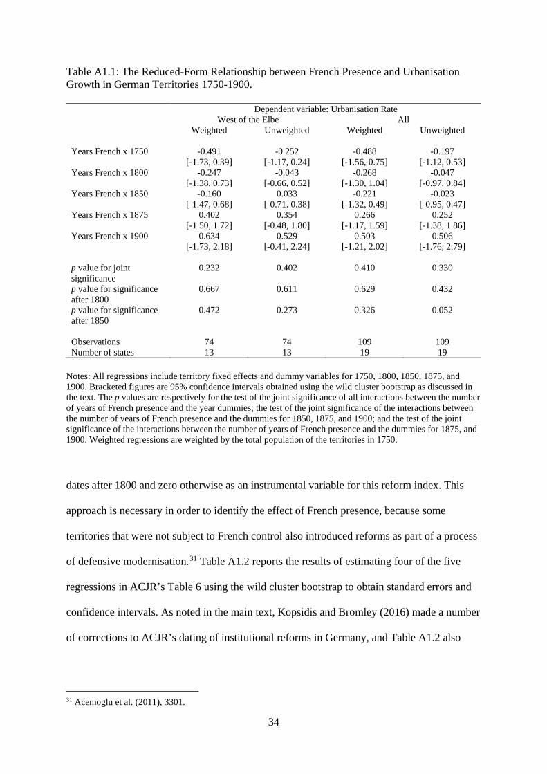
Table A1.1 reports the results of estimating the same regressions as in ACJR’s Table

3, but using the wild cluster bootstrap to obtain standard errors and confidence intervals.

These were calculated employing the Stata user-written command boottest of Roodman et al.

(2019). The number of replications in each case was 9,999 and the weights on the residuals

were drawn from the distribution proposed by Webb (2014). Table A1.1 follows ACJR in

presenting results for regressions weighted by the population of territories in 1750 as well as

unweighted regressions.

The point estimates of the terms which interact the number of years of French

presence with the five years from 1750 onwards show whether there was an association

between French presence in territories and urbanisation growth relative to the base year of

1700. The 95% confidence intervals obtained from the wild cluster bootstrap show that in all

four regressions these point estimates are estimated very imprecisely. The smallest of the four

p values for the test of the null hypothesis that all five interaction terms are zero is 0.232, so

that none of the four regressions provides any evidence of an effect of French presence on the

growth of urbanisation over the period as a whole. ACJR focus on the joint significance of

the three terms which interact French presence with the years after 1800, but the smallest of

the p values for this test is 0.432. Testing the joint significance of the two terms which

interact French presence with the years after 1850 does produce one p value of 0.052, but the

smallest of the other three is 0.273. The conclusion from Table A1.1 is that ACJR’s data are

uninformative about the association between French presence and urbanisation.

To establish a causal relationship between institutional reforms imposed by France

and urbanisation growth, ACJR constructed an index of reforms in all 19 territories, and used

the number of years of French presence interacted with a linear time trend that is positive for

34

Table A1.1: The Reduced-Form Relationship between French Presence and Urbanisation Growth in German Territories 1750-1900.

Dependent variable: Urbanisation Rate West of the Elbe All Weighted Unweighted Weighted Unweighted Years French x 1750 -0.491 -0.252 -0.488 -0.197 [-1.73, 0.39] [-1.17, 0.24] [-1.56, 0.75] [-1.12, 0.53] Years French x 1800 -0.247 -0.043 -0.268 -0.047 [-1.38, 0.73] [-0.66, 0.52] [-1.30, 1.04] [-0.97, 0.84] Years French x 1850 -0.160 0.033 -0.221 -0.023 [-1.47, 0.68] [-0.71. 0.38] [-1.32, 0.49] [-0.95, 0.47] Years French x 1875 0.402 0.354 0.266 0.252 [-1.50, 1.72] [-0.48, 1.80] [-1.17, 1.59] [-1.38, 1.86] Years French x 1900 0.634 0.529 0.503 0.506 [-1.73, 2.18] [-0.41, 2.24] [-1.21, 2.02] [-1.76, 2.79] p value for joint significance

0.232 0.402 0.410 0.330

p value for significance after 1800

0.667 0.611 0.629 0.432

p value for significance after 1850

0.472 0.273 0.326 0.052

Observations 74 74 109 109 Number of states 13 13 19 19

Notes: All regressions include territory fixed effects and dummy variables for 1750, 1800, 1850, 1875, and 1900. Bracketed figures are 95% confidence intervals obtained using the wild cluster bootstrap as discussed in the text. The p values are respectively for the test of the joint significance of all interactions between the number of years of French presence and the year dummies; the test of the joint significance of the interactions between the number of years of French presence and the dummies for 1850, 1875, and 1900; and the test of the joint significance of the interactions between the number of years of French presence and the dummies for 1875, and 1900. Weighted regressions are weighted by the total population of the territories in 1750.

dates after 1800 and zero otherwise as an instrumental variable for this reform index. This

approach is necessary in order to identify the effect of French presence, because some

territories that were not subject to French control also introduced reforms as part of a process

of defensive modernisation.31 Table A1.2 reports the results of estimating four of the five

regressions in ACJR’s Table 6 using the wild cluster bootstrap to obtain standard errors and

confidence intervals. As noted in the main text, Kopsidis and Bromley (2016) made a number

of corrections to ACJR’s dating of institutional reforms in Germany, and Table A1.2 also

31 Acemoglu et al. (2011), 3301.

35

reports the results of estimating these regressions with the ACJR reform index replaced by

one constructed on the basis of the Kopsidis-Bromley (henceforth KB) corrections.32

Table A1.2 reports both instrumental-variable and OLS estimates of each regression

equation. It also reports the first-stage F statistic for the instrumental-variable estimates, and

the p value of a control function version of the Hausman test of whether the reform index can

be treated as an exogenous regressor: this is robust to clustering at the territory level and is

implemented using the wild cluster bootstrap. When the ACJR reform index is used, the first-

stage F statistics show no evidence of weak-instrument problems, and there is no evidence

that the ACJR index needs to be treated as an endogenous regressor. Inference can therefore

be based on the OLS estimates. The effect of the ACJR reform index is imprecisely estimated

in the weighted OLS regressions both for the territories west of the Elbe and for the sample

that also includes the east-Elbian territories. However, both the unweighted OLS regressions

yield estimates of the effect of the ACJR reform index which suggest that it probably had a

positive effect on urbanisation growth in the nineteenth century, although the 95% confidence

interval is sufficiently wide that it includes both economically quite large effects and effects

that are essentially zero.

I do not consider the reasons for this difference between the weighted and unweighted

regression estimates of the effect of the ACJR index further, because the estimates of the KB

reform index show that, when the ACJR index is corrected, the limited evidence of an effect

of the reforms disappears. The first-stage F statistics in this case are lower than when the

ACJR index is used, although there is only one regression for which the F statistic is low

enough as to suggest that weak-instrument problems might arise. There are greater

differences between the instrumental-variable and OLS point estimates of the effect of the

KB index than of the ACJR index, although none of the p values for the test of exogeneity of

32 Kopsidis and Bromley (2016), 164-168.

36

Table A1.2: Estimates of the Causal Effect of Reforms on Nineteenth-Century Urbanisation Growth in German Territories

Dependent Variable: Urbanisation Rate West of the Elbe Weighted Unweighted IV OLS IV OLS Reforms measured by ACJR index ACJR reforms index 0.291 0.281 0.204 0.220 [-0.30, 0.65] [-0.14, 0.45] [-0.13, 0.58] [-0.01, 0.49] p value of exogeneity test 0.925 - 0.847 - First-stage F statistic 119.72 - 61.85 - Reforms measured by KB index KB reforms index 0.511 0.230 0.369 0.234 (-∞, ∞) [-0.41, 0.71] (-∞, ∞) [-0.10, 0.66] p value of exogeneity test 0.132 - 0.420 - First-stage F statistic 31.32 - 24.85 - Observations 74 74 74 74 Number of states 13 13 13 13 All Weighted Unweighted IV OLS IV OLS Reforms measured by ACJR index ACJR reforms index 0.284 0.268 0.193 0.191 (-∞, ∞) [-0.12, 0.47] [-0.49, 0.81] [-0.002, 0.45] p value of exogeneity test 0.875 - 0.987 - First-stage F statistic 87.58 - 43.71 - Reforms measured by KB index KB reforms index 0.549 0.179 0.384 0.146 (-∞, ∞) [-0.34, 0.61] (-∞, ∞) [-0.15, 0.45] p value of exogeneity test 0.372 - 0.461 - First-stage F statistic 21.78 - 12.96 - Observations 109 109 109 109 Number of states 19 19 19 19

Notes: All regressions include territory fixed effects and dummy variables for 1750, 1800, 1850, 1875, and 1900. Figures in brackets and parentheses are 95% confidence intervals obtained using the wild cluster bootstrap as discussed in the text. Weighted regressions are weighted by the total population of the territories in 1750.

the KB index are low enough to suggest that the difference is statistically significant. But the

point estimates of the effect of the KB reform index are all very imprecise. This is especially

the case for the instrumental-variable estimates, for which all four 95% confidence intervals

37

are (-∞, ∞).33 But even the OLS point estimates are very poorly determined. The conclusion

from Table A1.2 is that any evidence of a positive causal effect of institutional reforms

imposed by France disappears once the KB corrections to the ACJR reform index are taken

into account. As with ACJR’s reduced-form regressions, there is no evidence from the

instrumental-variable regressions that the French presence in German territories had positive

effects on the growth of urbanisation. ACJR’s data are simply not detailed enough to provide

any evidence in support of their claim.

A2. Pre-Nineteenth-Century Institutional Variation and Nineteenth-Century Economic Development in Prussia

Section 2 of the main text discusses the differences in the institutional framework for

economic activity in Prussia which existed before the French invasion. This section expands

on that discussion. It also compares the Rhineland and Silesian textile industries to provide a

specific illustration of how different institutional frameworks resulted in different nineteenth-

century experiences for industrial regions that already existed in Germany at the end of the

eighteenth century.

Throughout the territories that comprised later nineteenth-century Prussia, economic

activity in both the early modern period and the nineteenth century was constrained by

institutions, but there was considerable variation between these territories. In rural areas,

these constraints involved manorial systems with powerful landlords and village

communities; in urban areas, craft guilds, merchant associations, and towns themselves; and

in both areas, the state, which played an important role in enforcing the privileges of urban

and rural institutions. Repeated military crises throughout the seventeenth and eighteenth

centuries led the rulers of many of these territories to grant privileges to the groups within

33 The range of values actually considered was -10,000 to 10,000.

38

their societies on which they depended for fiscal, military, administrative, and political

support. The importance of the state in enforcing institutional privileges combined with the

territorial fragmentation of the Holy Roman Empire meant that the institutional framework

could vary greatly over short distances. In the Rhineland (most of which was not Prussian

until 1815), for example, there were eight distinct sovereign rulers in the seventeenth century.

This fragmentation enabled early industries easily to cross territorial boundaries in order to

locate where institutional conditions were least oppressive.

There was substantial regional variation in the importance of the different institutions

that affected economic activity. Serfdom was stronger east of the river Elbe, where landlords

were powerful, demesne farms were large, labour dues were heavy, serf mobility was

restricted, and serfs’ decisions about the allocation of the labour they retained for their own

use were often subject to restrictions imposed by landlords. In the west, landlords were

typically less powerful and received revenue mainly from cash rents paid by tenants who

were mostly free. But there was some variation in landlord power west of the Elbe. In the

Rhineland, landlord power had declined sufficiently by the sixteenth century to allow flexible

land use, livelier commerce, more open rural goods markets, and the operation of labour

markets unconstrained by serfdom.34 However, in parts of Westphalia landlords were able to

influence land use and the size of the rural industrial labour force at least until the abolition of

the communal-manorial system of regulating agriculture, which occurred in 1770 in the

Prussian-ruled county of Ravensberg, but not until 1810 in the neighbouring prince-bishopric

of Osnabrück. The successful factory industrialisation of Ravensberg in the nineteenth

century, when most other Westphalian linen districts de-industrialised, is attributed partly to

the early abolition of communal-manorial agricultural regulation there.35

34 Kisch (1959), 555; Ogilvie (1996b), 283. 35 Ogilvie (1996b), 283.

39

Strong village communities could constrain economic activity by regulating markets

in most commodities, enforcing the privileges of rural guilds, and restricting migration,

marriage and settlement. These communities tended to be stronger west of the Elbe, where

landlords were weaker, but there were regional exceptions. In many areas of the Rhineland

village communities were weak from before the sixteenth century. But in Westphalia the

communal-manorial agrarian system gave village communities as well as landlords the power

to regulate land and labour markets, with harmful effects on industrial growth that have

already been noted.36

The privileges of towns, guilds, and merchant associations also constrained economic

activity. In parts of the Rhineland, such as Krefeld and Monschau, the weakness of such

constraints enabled the growth of highly successful textile industries (in silk and fine woollen

fabrics respectively). But elsewhere in the Rhineland these constraints were stronger and

hampered economic development. Guild restrictions on production resulted in the stagnation

of the Aachen woollen industry in the eighteenth century, and guild opposition to new

techniques led scythe-makers in Remscheid and cutlery-makers in Solingen to fall behind

their western European competitors. The Wuppertaler Garnnahrung, a powerful merchant

association, was granted privileges over bleaching and trading linen in the Wupper valley by

the Dukes of Berg in 1527 and continued to regulate the regional textile industry in its own

interests until the beginning of the nineteenth century. The mechanised spinning mill which

was opened in the Rhineland town of Ratingen in 1784 by a merchant called Jan Brügelmann

is regarded by Hardach (1991) as marking the beginning of the German industrial revolution.

However, Brügelmann had first tried to set up this mill in the Wupper valley in 1782.

Determined opposition by the Wuppertaler Garnnahrung and the rural weavers’ guild meant

36 Ogilvie (1996b), 284.

40

that when he did get a state monopoly concession two years later the mill was built outside

the Wupper valley.37

In Westphalia, the linen export trade was a legal monopoly of urban merchants

because of a law requiring rural spinners and weavers to sell through inspection offices in the

towns. Most of these inspection offices were strengthened by rulers in the 1770s and survived

into the nineteenth century. Ravensberg’s successful transition to factory industrialisation

around 1850, while other Westphalian linen regions de-industrialised, is partly ascribed to the

operation of illegal rural traders made possible by its less thorough enforcement of the

requirement to sell through inspection offices.38

As a result of differences in the institutional framework for economic activity, the

west of Prussia was more economically advanced than the east at the end of the eighteenth

century, although the continued existence of some traditional institutions meant that the

Rhineland and Westphalia lagged behind England. Of the 16 industrial regions in Prussia

around 1800 identified by Kaufhold (1986), 14 were in the west – in Rhineland and

Westphalia – and only two were in the east, in Silesia.

The following comparison of the development of the textile industry in the Rhineland

and Silesia, which draws heavily on Kisch (1959), throws further light on the role of pre-

1800 institutional differences for nineteenth-century economic development. In both the

Rhineland and Silesia, linen production developed in the sixteenth century, and by the

seventeenth century both regions were supplying linen to the north Atlantic economies.39

Subsequently the Rhineland expanded its textile production into cotton, silk, and woollen

cloth, but linen continued to constitute almost all Silesia’s textile exports throughout the

eighteenth century. During the nineteenth century, textile production became mechanised in

37 Ogilvie (1996b), 286-7. 38 Ogilvie (1996b), 288-9. 39 Kisch (1959), 543; Ogilvie (1996b), 264-5.

41

the Rhineland and continued to play an important role in the region’s economic development,

but in Silesia the textile industry stagnated. The Rhineland had the advantage of being located

nearer the Netherlands and England than Silesia, but Silesia’s less favourable location did not

prevent its linen being exported to these economies in the seventeenth and eighteenth

centuries, so location cannot be the explanation of the nineteenth-century decline of the

Silesian linen industry.

As already noted, the institutional framework in the Rhineland imposed

comparatively few constraints on economic activity. Thus it was possible for people to set up

textile firms and respond to new opportunities, such as the demand for cotton and silk,

without great difficulty. Some of these textile entrepreneurs became very successful and

accumulated the capital required to undertake the technological advances in textile

production that developed at the end of the eighteenth and the beginning of the nineteenth

century.40 The introduction of mechanised textile production methods did face opposition, as

Brügelmann’s problems in setting up his spinning mill reveal, but this example also shows

that the introduction of new technologies in the Rhineland was possible. Thus Rhineland

textile production was able to develop into a mechanised manufacturing industry in the

nineteenth century.41

In Silesia, one of the areas east of the Elbe which experienced the state-supported

expansion of landlord powers known as the “second serfdom” from the later sixteenth

century onwards, the ties of serfdom were much stronger. The development of Silesian linen

production therefore required the consent of landlords, which was given because the linen-

producing part of Silesia had low agricultural fertility. Landlords therefore gained more by

allowing their serfs to work in the linen proto-industry rather than in agriculture, extracting

40 Kisch (1959), 555-7. 41 Kisch (1959), 559-62.

42

revenues in a variety of ways such as loom and cloth fees; compelling serfs to work at low

wages; and, most importantly, by having the monopsony right to purchase the products of

their subjects, which they either exploited themselves or ceded to third parties such as

merchant associations in exchange for large fees.42 The low prices which made Silesian linen

internationally competitive in the seventeenth and for much of the eighteenth century derived

from the strong seigneurial institutions in Silesia, which enabled landlords coercively to

reduce labour costs. However, by the late eighteenth and early nineteenth centuries, the cost

advantage of Silesian linen had largely disappeared because of competition from English

cotton and mechanised production.43 In order to remain internationally competitive, it was

necessary to mechanise Silesian linen production or shift to mechanised cotton

manufacturing, but such technological changes were opposed by the landlords, who wished to

maintain the revenues they extracted from their linen-producing serfs. The landlords

persuaded the Prussian state to prohibit linen mechanisation. Furthermore, from the 1760s, a

state credit institution, the Landschaft, channelled almost all Silesian savings to the feudal

landlords, so that there were no funds for investment in industrial machinery.44 The result

was that the Silesian linen proto-industry withered away in the nineteenth century instead of

becoming a fully-fledged mechanized industry.

A3. Measures of Urbanisation

This section explains how my use of urbanisation as a measure of economic outcomes

differs from that of LO. In their Appendix A, LO conduct a number of checks of the

robustness of their baseline regression model, one of which is to use the urban population in a

42 Ogilvie (1997), 407. 43 Kisch (1959), 547-8. 44 Kisch (1959), 550-1.

43

county in 1871 as a measure of county economic outcomes. However, the results they report

using this measure (in their Table A4) are obtained not from their baseline regression model,

but from a regression model which adds two regressors to the baseline model: the urban

population in 1816 and the total population in 1816. LO do not explain why their baseline

model is modified in this way when the urban population in 1871 is the dependent variable.

Furthermore, LO’s use of the urban and total population in 1816 as regressors reduces the

number of observations substantially, to 291.

There is another curious feature of the regression that LO estimate using the urban

population in 1871 as the dependent variable. One of the regressors is the fraction of the

county population in 1871 which lived in towns of more than 2,000 inhabitants, which, for

brevity, I call the urbanisation rate in 1871. Since LO’s regression also includes the total

county population in 1871 as a regressor, it is unclear why the urbanisation rate in 1871

should also be a regressor. This variable is a regressor in LO’s baseline regression

specification, and it may have been included as a regressor when the urban population in

1871 is the dependent variable simply for that reason. However, the presence of this regressor

makes it difficult to interpret the results of LO’s regression with the urban population in 1871

as the dependent variable, and LO offer no explanation of why it is included in their

urbanisation regression. More generally, as noted in the main text, the urbanisation rate in

1871 is a bad control: it is a variable that is a potential outcome of the French institutional

reforms.

By contrast, the natural urbanisation variable to use as a measure of county economic

outcomes is the urbanisation rate in 1871. It is available for all 447 counties in LO’s dataset,

and I use it as an economic outcome measure throughout the paper.

44

A4. Omitted Variable Bias in the LO Baseline Model

This section provides a detailed analysis of the LO baseline regression model

(equation (5) of Table 3 in LO 2009). The economic outcome measure used in this regression

is the log of teacher income, and the culture measure is the share of Protestants. In Table 5 of

their paper, LO report the results of using six alternatives to the share of Protestants as

measures of cultural similarity to France in this baseline model. They conclude that the six

alternative measures of cultural similarity all confirm the results obtained using the share of

Protestants.

Three of LO’s alternative culture measures are based on the relationship between

French and the languages spoken in Prussian counties. The first of these measures, linguistic

distance, is constructed using information about the languages currently spoken in France and

regions that were Prussian in the nineteenth century. The second measure is an ordinal

version of linguistic distance, the ranking implied by the first measure. The third measure,

ancestral linguistic distance, uses information from an ancestral language map to identify the

languages in France and Prussian counties and calculates linguistic distance accordingly.45

The other three alternative culture measures are based on the attitudes to French

culture held by the eighteenth-century rulers of the territories that constituted later-

nineteenth-century Prussia. The no-French-ties dummy variable is zero if any one of four

conditions indicating a relationship with France applies to the eighteenth-century pre-

Napoleonic rulers of a Prussian county, and one otherwise. The no-French-ties index weights

the no-French-ties dummy by the number of years a ruler was in power in the period 1701-

1790. The French exposure dummy variable is one if either local rulers in the period 1701-90

had direct French relatives or there were Huguenot migrants in the county; Huguenots were

45 LO (2019), 1086-8, Appendix B.

45

French Calvinists, often invited by eighteenth-century German rulers to settle in their realms

in order to transmit manufacturing expertise.46 In contrast to the six other culture measures

used by LO, an increase in French exposure corresponds to a higher, not lower, cultural

similarity. In the discussion that follows, I use a no-French-exposure dummy variable,

defined as one minus the LO French exposure dummy, so that all culture measures have the

characteristic that increases in their value imply greater cultural dissimilarity with France.

Panel A of Table A4.1 shows, for each of the seven culture measures used by LO, the

estimated effects of French-imposed reforms and the interaction between Napoleon and the

measure of culture on the log of teacher income in the LO baseline model. These results

replicate those in Table 3 (equation (5)) and Table 5 of LO 2019.47 The point estimates of the

effect of French reforms when cultural similarity with France was greatest are positive for all

seven culture measures, and are precisely estimated in all cases except when culture is

measured by the no-French-exposure dummy. The point estimates of the term which interacts

Napoleon and the measure of culture are all negative and precisely estimated. The point

estimates of the effect of French reforms when cultural dissimilarity with France was greatest

are negative for all seven culture measures, and again these are precisely estimated except

when culture is measured by the no-French-exposure dummy.

However, the Moran test shows evidence of spatial correlation in the errors of all

seven regressions in panel A of Table A4.1. There is no evidence of spatial correlation in the

errors of the seven regressions in panel B of Table A4.1, which differ from those in panel A

only by including longitude as a regressor.48 In all seven regressions in panel B of Table

A4.1, longitude has a negative and precisely estimated effect. The estimated effects of French

reforms when the cultural similarity with France was greatest are very different from those in

46 LO (2019), 1088-9, Appendix B. 47 Recall that I use the no-French-exposure rather than the French exposure dummy. 48 To keep the argument as simple as possible, the regressions in panel B of Table A4.1 do not include the interaction of Napoleon with longitude as a regressor.

46

Table A4.1: Omitted Variable Bias in the LO Baseline Model

Measure of cultural similarity to France Protestant Share Linguistic

Difference Rank of

Linguistic Difference

Ancestral Linguistic Difference

No French Ties Dummy

No French Ties Index

No French Exposure Dummy

A. Omitting longitude Napoleon (Cult. Var. = Min) 0.144 0.056 0.115 1.251 0.056 0.087 0.055 [0.09, 0.20] [0.00, 0.11] [0.05, 0.18] [0.27, 2.23] [0.01, 0.10] [0.04, 0.13] [-0.01, 0.12] Napoleon (Cult. Var. = Max) -0.064 -0.832 -0.126 -0.080 -0.305 -0.190 -0.016 [-0.12, -0.01] [-1.48, -0.18] [-0.19, -0.06] [-0.17, 0.01] [-0.37, -0.24] [-0.27, -0.11] [-0.06, 0.03] Napoleon x Cult. Var. -0.208 -0.013 -0.0005 -0.201 -0.361 -0.523 -0.070 [-0.29, -0.13] [-0.02, -0.00] [-0.001, -0.000] [-0.36, -0.04] [-0.44, -0.28] [-0.69, -0.36] [-0.13, -0.01] p value of Moran test 0.000 0.000 0.000 0.000 0.000 0.000 0.000 Adjusted R2 0.654 0.634 0.645 0.636 0.709 0.664 0.635 B. Including Longitude Napoleon (Cult. Var. = Min) -0.002 -0.060 0.006 -0.222 0.016 0.017 0.044 [-0.06, 0.05] [-0.11, -0.01] [-0.05, 0.06] [-1.16, 0.71] [-0.04, 0.07] [-0.03, 0.07] [-0.02, 0.11] Napoleon (Cult. Var. = Max) -0.049 0.246 -0.088 -0.028 -0.248 -0.128 -0.052 [-0.10, 0.00] [-0.23, 0.72] [-0.15, -0.03] [-0.11, 0.06] [-0.31, -0.18] [-0.21,-0.04] [-0.09, -0.01] Napoleon x Cult. Var. -0.045 0.005 -0.0002 0.030 -0.264 -0.273 -0.096 [-0.12, 0.03] [-0.003, 0.012] [-0.0004,

-0.0000] [-0.12, 0.18] [-0.36, -0.17] [-0.46, -0.09] [-0.15, -0.04]

Longitude -0.012 -0.012 -0.012 -0.012 -0.008 -0.010 -0.012 [-0.014, -0.009] [-0.014, -0.010] [-0.014, -0.009] [-0.014, -0.010] [-0.011, -0.005] [-0.013, -0.007] [-0.014, -0.009] p value of Moran test 0.621 0.653 0.613 0.724 0.664 0.676 0.708 Adjusted R2 0.713 0.702 0.707 0.701 0.737 0.696 0.706

Notes: The dependent variable in all regressions is the logarithm of teacher income. The number of observations for all regressions is 447. All regressions include as regressors the culture variable, the geographical, historical, educational, and socio-economic control variables used by LO, and the interactions between the Napoleon dummy variable and the geographical and historical controls (LO 2019, 1074-6). The coefficients of these variables are not reported. The point estimates of Napoleon when the culture variables are at their minimum and maximum values are obtained by setting all other variables with which Napoleon is interacted except the culture variable to their sample mean values, and the culture variable to its sample minimum or maximum value as appropriate. The figures in brackets are 95% confidence intervals obtained from heteroscedasticity-robust estimates of the covariance matrix.

47

panel A in all cases except when culture is measured by the no-French-exposure dummy. In

the other six cases, the positive and precisely-estimated point estimates in panel A change to

become economically and statistically insignificant in four cases; economically significant,

negative, but imprecisely estimated in a fifth; and, in the sixth, negative and economically

and statistically significant. The point estimates of the term which interacts Napoleon and the

measure of culture are smaller (in absolute value) than those in panel A in all cases except

when culture is measured by the no-French-exposure dummy. When culture is measured by

the share of Protestants or the three measures based on linguistic distance, these point

estimates are imprecisely estimated, and positive in two cases. In panel B, the estimated

effects of French reforms when the cultural dissimilarity with France was greatest are not, in

most cases, very different from those in panel A. But the results in panel B of Table A4.1

show that, once the deeply rooted west-east difference in economic outcomes is taken into

account by including longitude as a regressor, there is no evidence that French reforms had

any positive effect on log teacher income. The claim that the term which interacts Napoleon

and the measure of cultural dissimilarity to France has a negative economic effect is not

robust to different culture measures.

The reason for the difference between the results in panel A and those in panel B of

Table A4.1 is clear from Table A4.2. This table reports the results of estimating regressions

of longitude on the regressors in the various regressions in panel A of Table A4.1. Table A4.2

shows that, whichever measure of culture is used, the Prussian counties under French control

which were culturally similar to France were typically in the more western parts of Prussia

(as shown by the negative point estimates of Napoleon (Cult. Var. = Min)), while those that

were culturally dissimilar to France were typically in the more eastern parts (as shown by the

positive point estimates of Napoleon (Cult. Var. = Max)). When longitude is omitted, the

estimated effects of any regressors in LO’s baseline model that are correlated with longitude

48

Table A4.2: The Association between Longitude and the Napoleon Dummy Variable at Different Values of the Culture Variables

Measure of cultural similarity to France Protestant Share Linguistic

Difference Rank of

Linguistic Difference

Ancestral Linguistic Difference

No French Ties Dummy

No French Ties Index

No French Exposure Dummy

Napoleon (Cult. Var. = Min) -12.285 -9.626 -9.340 -121.531 -4.808 -7.331 -0.915 [-14.98, -9.59] [-12.27, -6.98] [-12.09, -6.60] [-150.86, -92.20] [-6.08, -3.54] [-8.73, -5.93] [-3.01, 1.18] Napoleon (Cult. Var. = Max) 1.255 89.192 3.237 4.225 6.749 6.438 -3.083 [-0.07, 2.58] [57.76, 120.62] [0.93, 5.55] [2.27, 6.19] [4.14, 9.36] [4.57, 8.30] [-4.42, -1.74] Napoleon x Cult. Var. 13.540 1.472 0.029 19.042 11.557 25.979 -2.168 [10.39, 16.69] [0.97, 1.97] [0.02, 0.04] [14.36, 23.72] [8.71, 14.70] [21.27, 30.69] [-4.49, 0.15]

Notes: The dependent variable in all regressions is longitude. The number of observations for all regressions is 447. All regressions include as regressors the culture variable, the geographical, historical, educational, and socio-economic control variables used by LO, and the interactions between the Napoleon dummy variable and the geographical and historical controls (LO 2019, 1074-6). The coefficients of these variables are not reported. The point estimates of Napoleon when the culture variables are at their minimum and maximum values are obtained by setting all other variables with which Napoleon is interacted except the culture variable to their sample mean values, and the culture variable to its sample minimum or maximum value as appropriate. The figures in brackets are 95% confidence intervals obtained from heteroscedasticity-robust estimates of the covariance matrix.

49

will be biased. As Table A4.2 shows, the effects of French reforms at the largest and smallest

values of cultural similarity, as well as the interaction between Napoleon and the culture

measure, are correlated with longitude, so the estimated effects of these variables in the LO

baseline regressions in panel A of Table A4.1 are biased. The bias is given by the product of

the relevant point estimate in Table A4.2 and the point estimate of longitude in the

corresponding equation in panel B of Table A4.1.49 In the case of Napoleon (Cult. Var. =

Min), for example, the point estimates in Table A4.2 are all negative, and the point estimates

of longitude in the corresponding equations in Table A4.1 are also all negative, so the omitted

variable bias in the point estimates of Napoleon (Cult. Var. = Min) in the LO baseline

regressions is always positive. As Table A4.1 shows, this bias is also typically large.

A5. Problems with LO’s Ruler Fixed Effects

One of the robustness checks carried out by LO in their Appendix is to add ruler fixed

effects to their baseline regression model in order to take account of unobserved effects, such

as the institutional setting, which may be present in all territories with a common ruler. LO

identify 37 different territories in 1789 which, by the later nineteenth century, were part of

Prussia. LO’s ruler fixed effects reflect the different rulers of these territories in 1789;

according to LO, there were 18 different rulers. However, LO’s assignment of territories to

rulers is factually inaccurate. Several territories that were ruled by the King of Prussia are

treated by LO as having a different ruler. The most serious error is LO’s treatment of

territories ruled by the Elector of Brandenburg as having a different ruler to territories ruled

by the King of Prussia. The Elector of Brandenburg and the King of Prussia were one and the

same. But there are also other errors. LO treat the county of Tecklenburg, which was Prussian

49 This follows from the omitted variable bias formula: see, for example, Angrist and Pischke (2009), 60.

50

from 1707, as being ruled by the Bishop of Münster, and the counties of Usedom-Wollin and

Kammin, which were Prussian from 1720, as being ruled by Sweden. They also treat the four

counties of Hohenzollern, which did not become Prussian until 1850, as part of Brandenburg.

A further problem is that LO categorise all territories with a religious ruler as forming

a group with a common ruler, namely “the Church”. But different religious rulers followed

different policies and fostered different institutions, so they cannot all be treated as forming a

single homogeneous group.

It would be possible to correct LO’s errors of categorisation in order to obtain a

correct set of ruler fixed effects as of 1789. But even if all counties were correctly allocated

to their rulers, it is very difficult to believe that they all were subject to the same unobserved

ruler-level effect. The counties ruled by the King of Prussia extended from Kleve in the west

(longitude 10.71) to Stallupönen in the east (longitude 39.4). The Kings of Prussia did not

pay as much attention to their relatively small number of far western possessions as they did

to their more numerous other territories (Tilly and Kopsidis 2020, 45), and this had

implications for the economic development of these regions. During the eighteenth century,

for example, the silk industry of Krefeld (longitude 11.45) became highly successful despite

receiving no support from the Prussian state, in contrast to the expensive failure of the state-

supported Berlin silk manufacture. The failure of the latter led the Comte de Mirabeau in the

1790s to write of the Krefeld industry, “Unhappy those manufactures if ever a Prussian king

should love them” (Ogilvie 2000, 115). Roughly 40% of the counties in LO’s dataset were

ruled by the King of Prussia in 1789, and these extended over much of the geographical area

of late-nineteenth-century Prussia. If regional effects influenced economic development, it is

very unlikely that they were constant across the entirety of the territories ruled by the King of

Prussia before the French invasion.

51

A natural way to take account of unobserved regional effects would appear to be to

treat them as operating at the level of the 37 pre-Napoleonic territories identified by LO.

However, the 37 pre-Napoleonic territories identified by LO include two artificial states

(“Imperial Cities” and “Independent Cities”) which collect together large numbers of

autonomous cities. As discussed in the main text, the interpretive basis for combining the

autonomous cities in this way is highly questionable. I therefore assigned each of these cities

to its closest 1789 territory, as shown in Table A5.1, to obtain an alternative set of 35 regions

at which unobserved effects operate. These are the regional fixed effects used in Table 3 of

the main text. However, the following section of the Appendix shows that the results of Table

3 of the main text are robust if either LO’s ruler fixed effects or LO’s territory fixed effects

including the two artificial states comprising autonomous cities are used instead.

Table A5.1: Assignment of Imperial and Independent Cities to Pre-Napoleonic Territories

Imperial cities Independent cities City Territory assigned City Territory assigned

Landkreis Aachen Austrian Netherlands Berent Kingdom of Prussia Stadtkreis Aachen Austrian Netherlands Deliztsch Electorate of Saxony Landkreis Danzig Kingdom of Prussia Landkreis Duisburg Duchy of Berg Stadtkreis Danzig Kingdom of Prussia Stadtkreis Duisburg Duchy of Berg Dortmund County of Mark Eckartsberga Electorate of

Brandenburg Frankfurt am Main County of Nassau Lippstadt County of Mark Gelnhausen Landgraviate of Hesse-

Kassel Mühlhausen Electorate of Saxony

Liebenburg Duchy of Brunswick-Wolfenbüttel

Nordhausen Electorate of Saxony

Wetzlar County of Nassau

A6. The Robustness of the Results to Alternative Specifications of Regional Fixed Effects

Table 3 in the main text reports the estimated effects of French reforms on economic

outcomes in Prussia using regression models that include regional fixed effects which, as

52

discussed in the previous section, are based on LO’s pre-Napoleonic territories, but do not

include the two artificial states comprising autonomous cities. To check that these estimates

are not sensitive to the particular specification of regional fixed effects, Table A6.1 reports

the estimated effects of French reforms obtained from regression models that have alternative

specifications of such fixed effects, as discussed in the previous section, but are otherwise

identical to the regression models used in Table 3 of the main text. The estimates in panel A

of Table A6.1 are from models in which LO’s ruler fixed effects are used, while those in

panel B are from models in which the fixed effects are LO’s pre-Napoleonic territories,

including the two artificial states comprising autonomous cities.

There are some differences between the point estimates in Table 3 and the

corresponding ones in Table A6.1, but the estimates in Table A6.1 yield essentially the same

conclusions about the effect of French reforms as do those in Table 3. A necessary condition

for the LO claim that French reforms had positive effects on long-term Prussian economic

outcomes when they were imposed in culturally similar parts of Prussia, but negative effects

when imposed in culturally dissimilar parts, is that the Napoleon x Protestant Share

interaction term should have a negative effect on county economic outcomes. However, in

panel A of Table A6.1 the point estimates of this term are all positive, and three of them are

both economically and statistically significant. In panel B, four of the five point estimates are

positive, all four being economically significant, and two being statistically significant. The

single negative point estimate is neither economically nor statistically significant. The

conclusion drawn from Table A6.1 is the same as that from Table 3: there is no evidence to

support the LO claim.

As for the effects of French reforms, all ten point estimates in Table A6.1 of the effect

of the reforms when the share of Protestants was zero are negative. Six of these are

economically significant, and five are statistically significant. Table A6.1 provides no

53

Table A6.1: The Effect of French Reforms on Economic Outcomes in Prussia with Alternative Regional Fixed Effects

Dependent variable Log teacher

income Income tax per capita.

Non-agric share

Log wage Urbanisation rate

A. LO ruler fixed effects Napoleon (Prot. Share=0) -0.043 -0.143 -10.161 -0.091 -0.099 [-0.13, 0.05] [-0.50, 0.21] [-17.35,

-2.98] [-0.18, -0.00] [-0.19, -0.01]

Napoleon (Prot. Share=1) 0.005 0.121 2.529 0.031 0.020 [-0.04, 0.05] [-0.15, 0.39] [-2.20, 7.26] [-0.03, 0.09] [-0.05, 0.09] Napoleon x Prot. Share 0.047 0.264 12.690 0.122 0.119 [-0.04, 0.14] [-0.11, 0.63] [4.57, 20.81] [0.02, 0.22] [0.01, 0.23] Longitude -0.012 -0.049 -0.744 -0.024 -0.005 [-0.017,

-0.008] [-0.07, -0.03] [-1.13, -0.66] [-0.029,

-0.019] [-0.01, -0.00]

p value of Moran test 0.938 0.583 0.724 0.491 0.318 p value of Mundlak test 0.000 0.000 0.001 0.000 0.000 Adjusted R2 0.623 0.428 0.517 0.695 0.592 Number of observations 445 419 445 427 445 B. LO regional fixed effects with two artificial city-based states Napoleon (Prot. Share=0) -0.018 -0.110 -10.095 -0.154 -0.067 [-0.10, 0.07] [-0.49, 0.27] [-17.72,

-2.47] [-0.24, -0.07] [-0.17, 0.03]

Napoleon (Prot. Share=1) -0.061 0.254 0.023 0.006 -0.014 [-0.14, 0.02] [-0.03, 0.54] [-4.40, 4.45] [-0.05, 0.06] [-0.08, 0.06] Napoleon x Prot. Share -0.043 0.364 10.117 0.160 0.053 [-0.12, 0.03] [-0.04, 0.77] [1.84, 18.39] [0.07, 0.25] [-0.06, 0.17] Longitude -0.014 -0.082 -0.691 -0.024 -0.002 [-0.018,

-0.009] [-0.11, -0.05] [-1.20, -0.18] [-0.031,

-0.017] [-0.009, 0.004]

p value of Moran test 0.359 0.333 0.367 0.475 0.239 p value of Mundlak test 0.000 0.000 0.001 0.000 0.001 Adjusted R2 0.680 0.474 0.599 0.747 0.638 Number of observations 443 417 443 426 443

Notes: All regressions include as regressors Protestant Share, a dummy for the presence of an Imperial city in the sixteenth century, a dummy for the presence of a Hanseatic city in the sixteenth century, urban population density in 1500, a dummy for being Polish-speaking, latitude, the log of county area, a dummy for the existence of coal deposits, the distance to Berlin, the distance to the district capital, an interaction between the Napoleon dummy and urban population density in 1500, and an interaction between the Napoleon dummy and a dummy for the existence of coal deposits. The regressions in which the dependent variable is the urbanisation rate also include an interaction between the Napoleon dummy and the dummy for being Polish-speaking, and an interaction between the Napoleon dummy and the log of county area. The coefficients of these variables are not reported. The point estimates of Napoleon when Protestant Share is zero and one are obtained by setting all other variables with which Napoleon is interacted except Protestant Share to their sample mean values, and Protestant Share to zero or one as appropriate. The figures in brackets are 95% confidence intervals obtained from heteroscedasticity-robust estimates of the covariance matrix.

evidence that French reforms had a positive effect in those parts of Prussia that were

culturally most similar to France. When the share of Protestants was one, all the five point

54

estimates of the effect of French reforms in panel A of Table A6.1 are positive, though none

are statistically significant and at best their economic significance is modest. In panel B, three

of the five point estimates of the effect of French reforms in this case are positive and two are

negative, but none of them are statistically significant and only one (when income tax per

capita is the dependent variable) is economically significant. Table A6.1, like Table 3 of the

main text, provides no evidence that French reforms had positive effects on long-term

Prussian economic development.

In equation 1 of their Table A6, LO report results from a regression in which ruler

fixed effects are added to the LO baseline model. LO interpret these results as showing that

their claim about the importance of cultural proximity for the effects of French reforms

continues to hold when unobserved ruler fixed effects are taken into account. This conflicts

with the results reported in Table A6.1 of the present paper, in which there is no evidence in

support of the LO claim from the regressions using ruler fixed effects.

The reason for this conflict is simple, as Table A6.2 shows. LO’s omission of

longitude as a regressor continues to bias their estimates even when ruler fixed effects are

taken into account. Table A6.2 reports the estimated effects of French reforms, and the

Napoleon x Protestant Share interaction term, from LO’s regression with ruler fixed effects,

which omits longitude, and from a regression that adds longitude as a regressor to the LO

ruler fixed effect regression. When longitude is omitted, the estimated effect of Napoleon x

Protestant Share is negative and both economically and statistically significant. French

reforms are estimated to have positive effects on the log of teacher income whatever the share

of Protestants, but the effect is larger when the share of Protestants was zero. However, the

inclusion of longitude completely changes these estimates. Longitude itself has a very

precisely estimated negative effect on teacher incomes even though ruler fixed effects are

taken into account. Once longitude is included, the estimated effect of Napoleon x Protestant

55

Table A6.2: LO Ruler Fixed Effect Estimates of the Effect of French Reforms Omitting and Including Longitude

LO baseline model with ruler fixed effects

LO baseline model with ruler fixed effects and

longitude Napoleon (Prot. Share=0) 0.136 0.024 [0.07, 0.20] [-0.04, 0.09] Napoleon (Prot. Share=1) 0.047 -0.003 [0.00, 0.09] [-0.05, 0.04] Napoleon x Prot. Share -0.088 -0.027 [-0.16, -0.01] [-0.10, 0.04] Longitude - -0.010 [-0.013, -0.006] p value of Moran test 0.386 0.539 Adjusted R2 0.764 0.780

Notes: The dependent variable is the log of teacher income and the number of observations is 445. All regressions include as regressors Protestant Share, the geographical, historical, educational, and socio-economic control variables used by LO, and the interactions between the Napoleon dummy variable and the geographical and historical controls, (LO 2019, 1074-6). The coefficients of these variables are not reported. The point estimates of Napoleon when Protestant Share was zero and one are obtained by setting all other variables with which Napoleon is interacted except Protestant Share to their sample mean values, and Protestant Share to zero or one as appropriate. The figures in brackets are 95% confidence intervals obtained from heteroscedasticity-robust estimates of the covariance matrix.

Share, though negative, becomes much smaller (in absolute value) and is not precisely

estimated, and there is no evidence of an economically or statistically significant effect of

French reforms, whatever the share of Protestants.

A7. Allowing for Different Durations of French-Imposed Reforms

As noted in the main text, 48 Prussian counties were under French control for 19

years, 183 for 6 years, and 7 for 3 years. In Table A7.1 I report the results of estimating

regression models which are the same as those in Table 3 of the main text except that the

single Napoleon dummy is replaced, both on its own and when interacted with other

regressors, by two different dummy variables, in order to allow the effect of French reforms

to differ according to the duration of French control. LongFr takes the value one for the 48

counties that were subject to French control for 19 years and is zero otherwise, while ShortFr

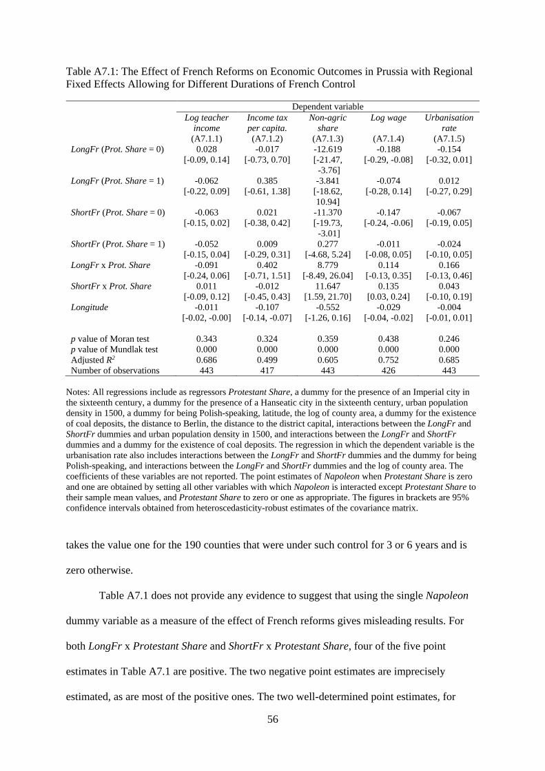
56

Table A7.1: The Effect of French Reforms on Economic Outcomes in Prussia with Regional Fixed Effects Allowing for Different Durations of French Control

Dependent variable Log teacher

income Income tax per capita.

Non-agric share

Log wage Urbanisation rate

(A7.1.1) (A7.1.2) (A7.1.3) (A7.1.4) (A7.1.5) LongFr (Prot. Share = 0) 0.028 -0.017 -12.619 -0.188 -0.154 [-0.09, 0.14] [-0.73, 0.70] [-21.47,

-3.76] [-0.29, -0.08] [-0.32, 0.01]

LongFr (Prot. Share = 1) -0.062 0.385 -3.841 -0.074 0.012 [-0.22, 0.09] [-0.61, 1.38] [-18.62,

10.94] [-0.28, 0.14] [-0.27, 0.29]

ShortFr (Prot. Share = 0) -0.063 0.021 -11.370 -0.147 -0.067 [-0.15, 0.02] [-0.38, 0.42] [-19.73,

-3.01] [-0.24, -0.06] [-0.19, 0.05]

ShortFr (Prot. Share = 1) -0.052 0.009 0.277 -0.011 -0.024 [-0.15, 0.04] [-0.29, 0.31] [-4.68, 5.24] [-0.08, 0.05] [-0.10, 0.05] LongFr x Prot. Share -0.091 0.402 8.779 0.114 0.166 [-0.24, 0.06] [-0.71, 1.51] [-8.49, 26.04] [-0.13, 0.35] [-0.13, 0.46] ShortFr x Prot. Share 0.011 -0.012 11.647 0.135 0.043 [-0.09, 0.12] [-0.45, 0.43] [1.59, 21.70] [0.03, 0.24] [-0.10, 0.19] Longitude -0.011 -0.107 -0.552 -0.029 -0.004 [-0.02, -0.00] [-0.14, -0.07] [-1.26, 0.16] [-0.04, -0.02] [-0.01, 0.01] p value of Moran test 0.343 0.324 0.359 0.438 0.246 p value of Mundlak test 0.000 0.000 0.000 0.000 0.000 Adjusted R2 0.686 0.499 0.605 0.752 0.685 Number of observations 443 417 443 426 443

Notes: All regressions include as regressors Protestant Share, a dummy for the presence of an Imperial city in the sixteenth century, a dummy for the presence of a Hanseatic city in the sixteenth century, urban population density in 1500, a dummy for being Polish-speaking, latitude, the log of county area, a dummy for the existence of coal deposits, the distance to Berlin, the distance to the district capital, interactions between the LongFr and ShortFr dummies and urban population density in 1500, and interactions between the LongFr and ShortFr dummies and a dummy for the existence of coal deposits. The regression in which the dependent variable is the urbanisation rate also includes interactions between the LongFr and ShortFr dummies and the dummy for being Polish-speaking, and interactions between the LongFr and ShortFr dummies and the log of county area. The coefficients of these variables are not reported. The point estimates of Napoleon when Protestant Share is zero and one are obtained by setting all other variables with which Napoleon is interacted except Protestant Share to their sample mean values, and Protestant Share to zero or one as appropriate. The figures in brackets are 95% confidence intervals obtained from heteroscedasticity-robust estimates of the covariance matrix.

takes the value one for the 190 counties that were under such control for 3 or 6 years and is

zero otherwise.

Table A7.1 does not provide any evidence to suggest that using the single Napoleon

dummy variable as a measure of the effect of French reforms gives misleading results. For

both LongFr x Protestant Share and ShortFr x Protestant Share, four of the five point

estimates in Table A7.1 are positive. The two negative point estimates are imprecisely

estimated, as are most of the positive ones. The two well-determined point estimates, for

57

ShortFr x Protestant Share in equations (A7.1.3) and (A7.1.4), are similar to the

corresponding point estimates for LongFr x Protestant Share. There is no evidence of a

general tendency for LongFr to have a positive effect on economic outcomes: when the share

of Protestants was zero, four of the five point estimates of the effect of LongFr are negative,

while three of the five point estimates of the effect of LongFr are negative when the share of

Protestants was one. The absolute values of the point estimates of the effect of LongFr do

tend to be larger than those of the effect of ShortFr: this is the case for three of the five pairs

of estimates when the share of Protestants was zero, and four of the five when the share of

Protestants was one. But there is no general tendency for the LongFr point estimates to be

positive and the ShortFr ones to be negative.

Most of the point estimates of the effects of LongFr and ShortFr are poorly

determined, and this raises the question of whether there is any clear evidence of differences

between them. The p values for the joint test of the null hypotheses that there was no

difference between the effects of LongFr and ShortFr both when the share of Protestants was

zero and when the share of Protestants was one were as follows: 0.228 in (A7.1.1), 0.748 in

(A7.1.2), 0.798 in (A7.1.3), 0.620 in (A7.1.4), and 0.519 in (A7.1.5). There is no evidence

that the effects of French reforms differed by the duration of French control.

A8. Alternative Measures of Cultural Similarity

LO’s main measure of the cultural distance between Prussian counties and France is

the share of Protestants, but they check the robustness of their results by using several

alternatives to religious affiliation as the basis for identifying cultural similarities. Three of

these alternatives are based on the linguistic difference between French and the languages

spoken in Prussian counties, and a further three are based on the attitudes to French culture

58

held by the eighteenth-century rulers of the territories that constituted later-nineteenth-

century Prussia.50 In order to investigate how the results in Table 3 of the main text depended

on the measure of culture, I estimated the regional fixed effect regression specifications in

that table using each of these six alternatives. These six culture measures, together with the

share of Protestants, mean that there are seven different sets of regression results for each

measure of county economic outcomes, and thus 35 sets of results altogether. What general

conclusions emerge from these?

I begin with the LO view that the sign of the term which interacts Napoleon with the

culture measure should show the effect of French reforms decreasing as cultural dissimilarity

increases. 18 of the 35 point estimates had a negative sign and were thus consistent with the

LO view. However, none of these 18 point estimates had a p value below 0.1. Only four of

the 35 point estimates of this interaction term had a p value below 0.1. These all had positive

signs and so were inconsistent with the LO view. Two of these four positive point estimates

with p values less than 0.1 were those in equations (3.3) and (3.4) of Table 3. The variation in

the sign of the point estimates of this interaction term across all 35 sets of results was

repeated within the seven sets of results for each particular economic outcome measure. For

two of the outcome measures the sign of the point estimate was the same for five of the seven

alternative culture measures, but for the other three outcome measures the point estimate took

one sign in four cases and the opposite sign in three. There was less variation in the sign of

the point estimates of the interaction term within alternative culture measures. The five point

estimates were all negative, and hence consistent with the LO view, for one of the seven

culture measures, though the p values were all above 0.1 in this case. For three other culture

measures four of the five point estimates were of the same sign, although this sign was

50 LO (2019), pp 1086-9.

59

inconsistent with the LO view for two of the measures. For the remaining three culture

measures, only three of the five point estimates were of the same sign.

This variation in the sign of the point estimates of the interaction between Napoleon

and the culture measures means that the specific point estimates of this interaction term in

Table 3 of the main text are not robust to the use of alternative culture measures. But this

variation also suggests strongly that the long-term impact of French reforms on Prussian

economic outcomes was not influenced by the cultural similarity between Prussian counties

and France. Table 3 shows that there is no evidence that this cultural similarity influenced

economic outcomes in the way LO claim, but it suggests that the interaction between

Napoleon and the culture measure might have had a positive effect on economic outcomes.

This conclusion is not supported by the robustness tests using other culture measures than the

share of Protestants, so the conclusion drawn from Table 3 should be limited to the absence

of evidence supporting the LO claim.

I now turn to the estimated effects of French reforms on economic outcomes in the

cases when cultural similarity to France was largest and smallest. When the cultural similarity

to France was greatest, 27 of the 35 point estimates are negative, of which eight had p values

below 0.1. All the eight positive point estimates had p values above 0.1. In the case of

greatest cultural dissimilarity to France, there were again 27 negative point estimates, six of

which had p values below 0.1. Once again, all the eight positive point estimates had p values

above 0.1. The total of 14 negative point estimates with p values below 0.1 were distributed

among all five economic outcome measures, though income tax per capita and the

urbanisation rate each had only one such estimate. These 14 point estimates were distributed

among six of the seven alternative culture measures: the measure based on ancestral linguistic

difference yielded no point estimate of the effect of French reforms with a p value below 0.1.

60

These alternative measures of the cultural difference between Prussian counties and

France strongly suggest that there is no clear evidence that French reforms influenced long-

term economic outcomes in Prussia. If there was any effect, the evidence suggests that it was

a negative one, a finding consistent with the results in Table 3.

61

Additional references for Appendix Cameron, A. C., J. B. Gelbach, and D. L. Miller (2008). “Bootstrap-based Improvements for Inference with Clustered Errors”, Review of Economics and Statistics, 90, 414-427. Carter, A. V., K. T. Schnepel, and D. G. Steigerwald (2017). “Asymptotic Behaviour of a t-test Robust to Cluster Heterogeneity”, Review of Economics and Statistics, 99, 698-709. Kisch, H. (1959). “The Textile Industries in Silesia and the Rhineland: A Comparative Study in Industrialization”, Journal of Economic History, 19, 541-564. Lee, C. H. and D. G. Steigerwald (2018). “Inference for Clustered Data”, The Stata Journal, 18, 447-460. Ogilvie, S. C. (2000). “The European Economy in the Eighteenth Century”, in T. C. W. Blanning (ed.), The Eighteenth Century: Europe 1688-1815. Oxford: Oxford University Press. Roodman, D., J. G. MacKinnon, M. Ø. Nielsen, and M. D. Webb (2019). “Fast and Wild: Bootstrap Inference in Stata using Boottest”, The Stata Journal, 19, 4-60. Webb, M. D. (2014). “Reworking Wild Bootstrap Based Inference for Clustered Errors”, Queen’s University, Department of Economics, Working Paper No. 1315. https:// ideas.repec.org/p/qed/wpaper/1315.html.