Embed Size (px)
Citation preview

Can Flares Contribute to the Total Solar Irradiance
Variations?
Matthieu Kretzschmar and T. Dudok de WitLPCE / CNRS, Université d'Orléans, France
“Flare contribution to TSI”, M. Kretzschmar et al. , SVECSE, Bozeman, June 2008

✤The response of TSI to flare.
✤How could flares contribute to the TSI variations ?
“Flare contribution to TSI”, M. Kretzschmar et al. , SVECSE, Bozeman, June 2008

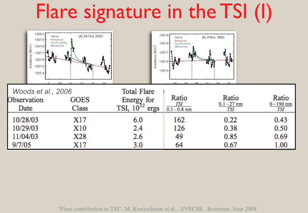
Flare signature in the TSI (I)
TSI signature observed for only 4 flares. This is because the TSI fluctuations (due to p-modes and convection) are about ~70ppm=0.1W/m2 and hide the emission increase due to flare.
Woods et al., 2006
“Flare contribution to TSI”, M. Kretzschmar et al. , SVECSE, Bozeman, June 2008
“Flare contribution to TSI”, M. Kretzschmar et al. , SVECSE, Bozeman, June 2008
Woods et al., 2006
Flare signature in the TSI (I)
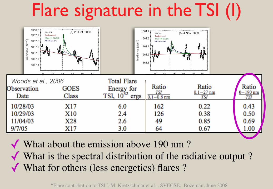
✓ What about the emission above 190 nm ?✓ What is the spectral distribution of the radiative output ?✓ What for others (less energetics) flares ?
“Flare contribution to TSI”, M. Kretzschmar et al. , SVECSE, Bozeman, June 2008
Woods et al., 2006
Flare signature in the TSI (I)

“Flare contribution to TSI”, M. Kretzschmar et al. , SVECSE, Bozeman, June 2008
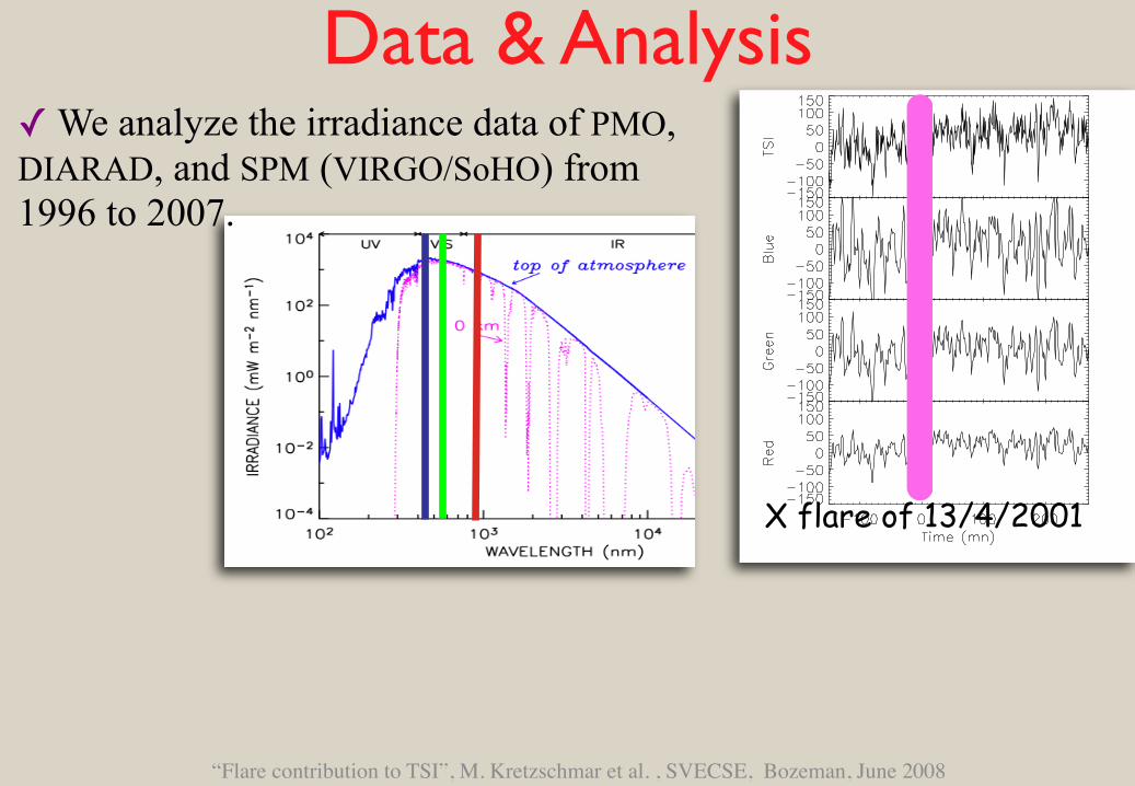
✓ We analyze the irradiance data of PMO, DIARAD, and SPM (VIRGO/SoHO) from 1996 to 2007.
Data & Analysis
“Flare contribution to TSI”, M. Kretzschmar et al. , SVECSE, Bozeman, June 2008
✓ We analyze the irradiance data of PMO, DIARAD, and SPM (VIRGO/SoHO) from 1996 to 2007.
X flare of 13/4/2001
Data & Analysis

“Flare contribution to TSI”, M. Kretzschmar et al. , SVECSE, Bozeman, June 2008
✓ We analyze the irradiance data of PMO, DIARAD, and SPM (VIRGO/SoHO) from 1996 to 2007.
To “see” the flares, we perform a conditional average or superposed epoch analysis:
1. Extract time series around each flare in the GOES db.2. Sum them: if random noise, it goes to zero.
X flare of 13/4/2001
Data & Analysis

Averaged total radiative output of large flare
Conditional average of TSI for all flares such that I0.1-0.8 > 10-4.3 W/m2 (X and strong M ones,)
“Flare contribution to TSI”, M. Kretzschmar et al. , SVECSE, Bozeman, June 2008
The TSI response to flares
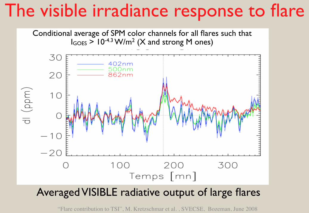
Averaged VISIBLE radiative output of large flares“Flare contribution to TSI”, M. Kretzschmar et al. , SVECSE, Bozeman, June 2008
The visible irradiance response to flareConditional average of SPM color channels for all flares such that
IGOES > 10-4.3 W/m2 (X and strong M ones)

1ppm ~0.0013 W/m^2 ~1.1 1030 ergs/s
IGOES > X2
M9.9 < IGOES < X2
M3.1 < IGOES < M9.9.
C9.9 < IGOES < M3.1
C1 < IGOES < C9.9
“Flare contribution to TSI”, M. Kretzschmar et al. , SVECSE, Bozeman, June 2008

IGOES > X2
M9.9 < IGOES < X2
M3.1 < IGOES < M9.9.
C1 < IGOES < C9.9
“Flare contribution to TSI”, M. Kretzschmar et al. , SVECSE, Bozeman, June 2008

10-4.5 < IGOES < 10-4.10-6. < IGOES < 10-5.
WL emission is ubiquitous during flare !!15 arcsec
1ppm in the irradiance ~ 20% contrast in 5 arcsec2. This agrees with other observations (Hudson, 2006)
White Light Flares
“Flare contribution to TSI”, M. Kretzschmar et al. , SVECSE, Bozeman, June 2008

Relative Optical and TSI increaseIGOES > 10-3.7
10-4 < IGOES < 10-3.7
10-4.5 < IGOES < 10-4.

“Flare contribution to TSI”, M. Kretzschmar et al. , SVECSE, Bozeman, June 2008
Energetics Confirm the value of Woods et al.(2006) for the effect of large flares on the TSI.
Large uncertainty for smaller flares, due to timing and statistics.
Red: random timing
Largest flares radiate about 1031-1032 ergs (in average, lower estimation)
Mea
n To
tal r
adia
tive
ener
gy [
Ergs
]
Rat
io T
otal
/ 0.
1-0.
8nm
Preliminary Conclusion✓ Flares do impact the TSI, even small ones.
✓ The emission at short (SXR, EUV) wavelengths during a flare constitutes a relatively small part of the total radiated energy (Egoes ~0.01 Etot for large flares).
✓ In particular, visible emission seems (quasi) systematic and to constitute an important contribution to the TSI increase.
✓ Largest flares have a total radiative energy of about 1032 ergs.
Could this imply a contribution of flares to long term (cycle) TSI variation ?
“Flare contribution to TSI”, M. Kretzschmar et al. , SVECSE, Bozeman, June 2008

Flare contribution to TSI variation (I)✓ TSI variations can be reproduced at about 90% by using the
changing areas of bright (plages..) and dark (spot). Last 10% ? Change from cycle to cycle ?
✓ The idea is: ‣ Each (nano)flare, in addition to heat the corona, produce an
emission at short wavelength (visible, near UV, IR) that has been neglected before.
‣ Heating of the corona requires a continuum of flares (Parker scenario).
‣ There is a natural modulation of the number (or the energy) of flares in phase with the solar cycle due to the heating of active region.
✓ Let’s quickly test this idea, neglecting many aspects.“Flare contribution to TSI”, M. Kretzschmar et al. , SVECSE, Bozeman, June 2008

Flare contribution to TSI variation (II)‣ Heating of the corona requires a continuum of flares (Parker
scenario).
“Flare contribution to TSI”, M. Kretzschmar et al. , SVECSE, Bozeman, June 2008
The number of observed flares at energy W follows a power law:
N(W ) = N1(W1
W)α
where ~ 1.8. This is valid between respectively the low and upper energy cut-off W1 and W2 such that ∫ W2
W1
WN(W )dW = Wtotis the energy released by all flares per unit of time and surface
W1,QS ~ W1,AR=1024erg; W2,QS~1030erg; W2,AR~1032ergWtot,qs~3.105 erg.cm-2.s-1; Wtot,AR~107 erg.cm-2.s-1 Aschwanden (2006)

dS ∼ f(W ) ∼ f(EGoes)
Flare contribution to TSI variation (II)‣ Each (nano)flare, produce an emission at short wavelength
(visible, near UV, IR) that has been neglected before.
“Flare contribution to TSI”, M. Kretzschmar et al. , SVECSE, Bozeman, June 2008
✓ We need a relation:
Mea
n To
tal r
adia
tive
ener
gy [
Ergs
]
10-4.5 < IGOES < 10-4.
✓Difficult ! ... still in progress..
We will assume
Or
dS ∼Wtot,AR

f(Wtot ∗ σAR(t))
Flare contribution to TSI variation (II)‣ modulation of the number (or energy) of flares.
“Flare contribution to TSI”, M. Kretzschmar et al. , SVECSE, Bozeman, June 2008
✓ With the active region we have a modulation of the energy:
✓ Two ways to estimate : •Use DSA (minimum estimate)•Use EIT/195 AR area from segmentation (Barra et al., in, preparation)
σAR(t)
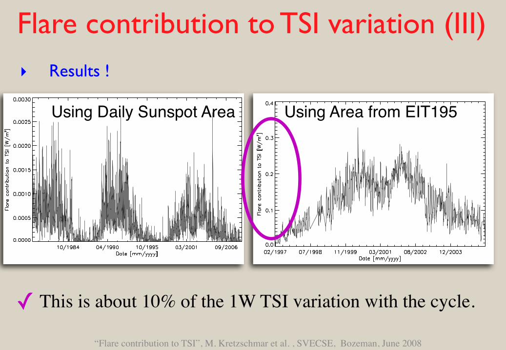
Flare contribution to TSI variation (III)‣ Results !
“Flare contribution to TSI”, M. Kretzschmar et al. , SVECSE, Bozeman, June 2008
Using Daily Sunspot Area Using Area from EIT195
✓ This is about 10% of the 1W TSI variation with the cycle.

Conclusion✓ Flares do impact the TSI, even small ones.
✓ Largest flares have a total radiative energy of about 1032 ergs.
✓ The emission at short (SXR, EUV) wavelengths during a flare constitutes a small part of the total radiated energy (Egoes ~0.01 Etot).
✓ In particular, visible emission seems (quasi) systematic and to constitute an important contribution to the TSI increase.
✓ Flares COULD contribute to the TSI variation, but probably not much.
“Flare contribution to TSI”, M. Kretzschmar et al. , SVECSE, Bozeman, June 2008
Thanks to W. Schmutz and S. Mekaoui for providing high cadence irradiance data !:
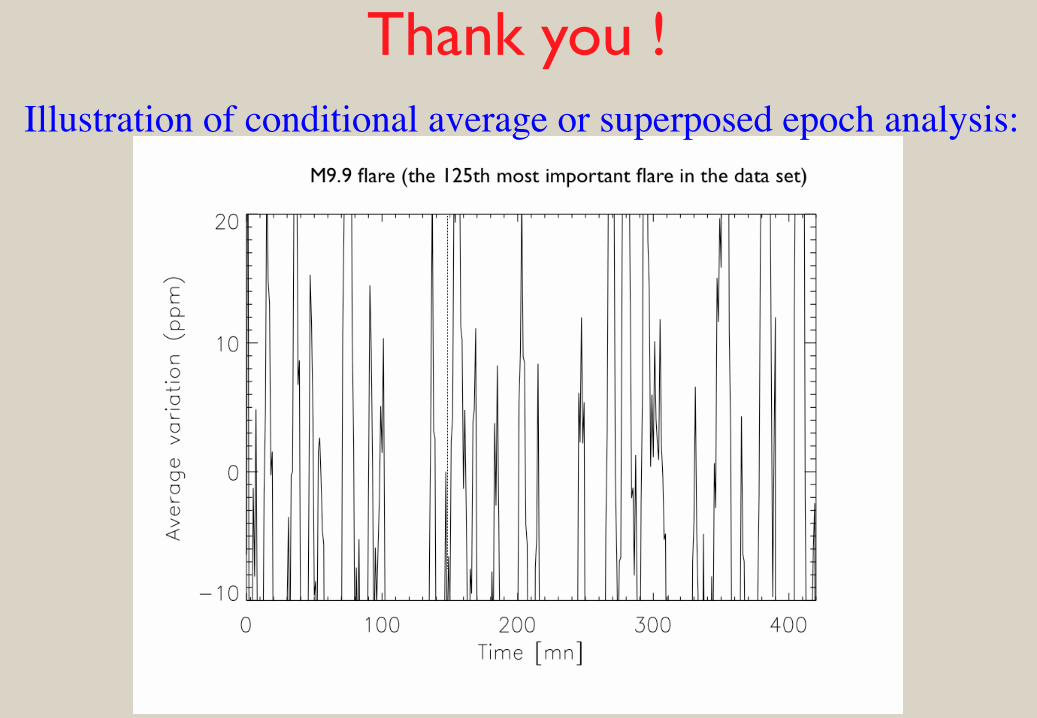
Thank you !Illustration of conditional average or superposed epoch analysis:

Backup slides
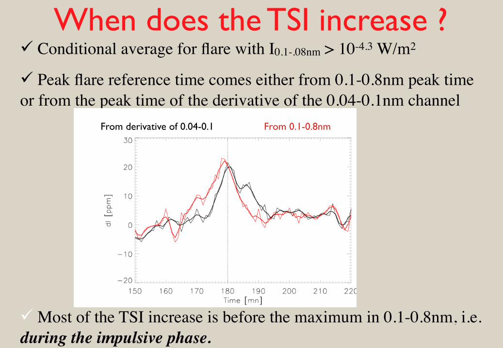
When does the TSI increase ? Conditional average for flare with I0.1-.08nm > 10-4.3 W/m2
Peak flare reference time comes either from 0.1-0.8nm peak time or from the peak time of the derivative of the 0.04-0.1nm channel
From derivative of 0.04-0.1 From 0.1-0.8nm
Most of the TSI increase is before the maximum in 0.1-0.8nm, i.e. during the impulsive phase.

where is the solar noise and is the signal due to the flare, e.g. . In the following, we concentrate on the time of the peak of the flare t0., such that yi(t0)=Si, and z=z(t0), x=x(t0).
xi(t) yi(t)
yi(t) = Si exp(− t− t0τi
)θ(t− t0)
Thus we can represent each time series as :
zi(t) = xi(t) + yi(t)
Our objective is that the signal becomes higher than the noise in the average time-series; it is then natural to average on the first n largest (as deduced from GOES classification) events, noted <...>n:
< z >n=n∑
i=1
zi =< x >n + < S >n
Conditional averaging: details (1/3)

We make the reasonable assumption that the xi are normally distributed with variance 2, thus:
< x >n∼ σ/√
n
and depends thus on the distribution function of the Si. If the average value decreases slower than n-1/2, then the SNR ratio increase. For Si, the reasonable assumption is to adopt the power law observed for flares at short wavelength:
f(S) ∼ C
S1+µ=
C
Sα, α ∼ 1.8
The ratio signal-over-noise of the averaged time-series is< S >n
< x >n=
1σ
√n < S >n
Conditional averaging: details (2/3)

Remember that we average the signal over the n largest flares, i.e. S1>S2>...>Sn and <S>n=1/n.i=1,n Si
The rank ordering statistics gives us the most probable values of the p-th variable Sp :
Conditional averaging: details (3/3)
Smpp =
[C(µN + 1)
µp + 1
] 1µ
And thus, Sn = (C(µN + 1))
1µ
1n
n∑
i=1
[1
µi + 1
] 1µ
Sn ∼1n
n∑
i=1
1
i1µ
or

Manual Movie

M9.9 flare (the 125th most important flare in the data set)

M9.9 flare + the 10 next

M9.9 flare + the 20 next

M9.9 flare + the 30 next

M9.9 flare + the 40 next

M9.9 flare + the 50 next
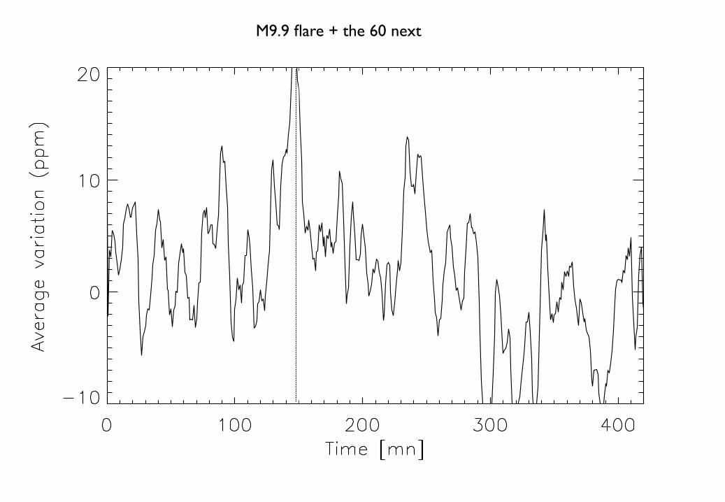
M9.9 flare + the 60 next

M9.9 flare + the 70 next

M9.9 flare + the 80 next

M9.9 flare + the 90 next
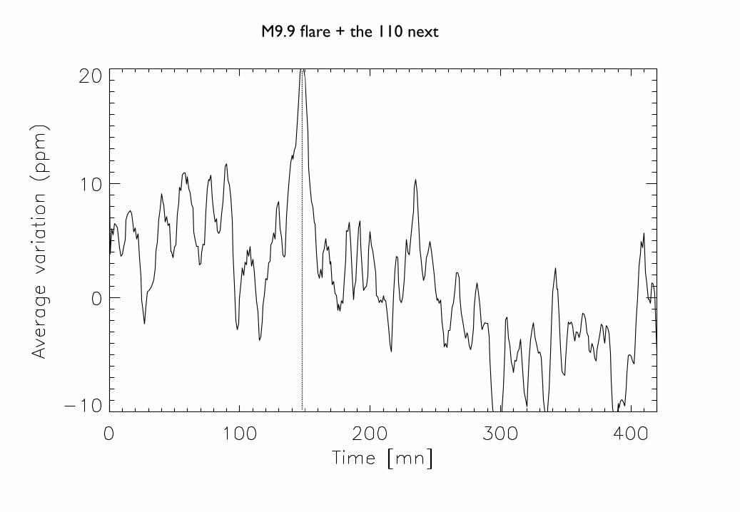
M9.9 flare + the 110 next
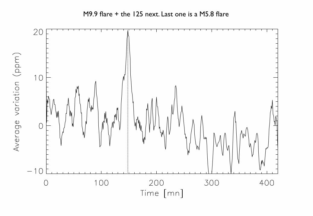
M9.9 flare + the 125 next. Last one is a M5.8 flare