Can Compensation Save Free Trade?†

Carl Davidson*, Steven J. Matusz*, and Douglas R. Nelson**

March 2004

Trade reform creates winners and losers. When the median voter loses from reform, free trade is blocked. Allowing the electorate to vote for compensatory wage or employment subsidies may lead to free trade under these circumstances. However, placing compensation on the agenda may also lead to an outcome where trade is blocked when it would have been supported otherwise. The reason for the latter result is that the transfer entailed under compensation is larger than the gains that the winners obtain from liberalization. Seeing the inevitable outcome of a series of votes, this group turns against liberalization.

* Michigan State University and GEP, University of Nottingham ** Tulane University and GEP, University of Nottingham Corresponding Author: Steven J. Matusz; Department of Economics; Michigan State University; East Lansing, MI 48824; Tel: 517-353-8719; Fax: 517-432-1068; Email: matusz@msu.edu. † We thank seminar participants at the University of Nottingham and Syracuse University for insightful comments on earlier drafts of this paper.

1

Introduction Welfare economics generally, and the welfare economics of international trade in

particular, has long understood that there is a close connection between liberalization and

the need for compensation. While liberalization generally implies gains, it also implies

adjustment, and, loosely speaking, the bigger the gains, the bigger the adjustment. We

have a sizable number of results, under quite general conditions, showing that free trade

dominates autarky and, under more restricted conditions, that existing forms of protection

could be liberalized in such a way as to produce an increase in aggregate economic

welfare. These results, however, rely on two fundamental abstractions: first, these are

long-run/comparative static results that do not consider the short-run costs of adjustment

from the distorted to the undistorted equilibrium; and, second, these results implicitly or

explicitly assume that compensation is carried out in such a way as to ensure that a

potential welfare gain is made actual. While both sorts of questions have produced

research seeking to evaluate the robustness of gains from trade results to their concerns,

in this paper we are interested in the positive political economy of the second question.1

The great majority of research on the positive political economy of domestic trade

policy can be seen as an attempt to answer the question: if protection is so bad, why is

there so much of it? The key result, presented most clearly in Mayer’s (1984)

fundamental paper: under the assumptions of the 2-good x 2-factor small HOS model,

with heterogeneity in household factor ownership, and determination of equilibrium

policy by simple referendum, except in the razors edge case in which the median

1 See Davidson and Matusz (2004) for an overview and extension of research on the first question. Fundamental normative research on the second question goes back to debates on the status of potential gain criterion of the Kaldor-Hicks sort, eventually evolving into questions about the feasibility of, and limits to, various compensation schemes. Examples of this latter research include Dixit and Norman (1986), Kemp

2

household factor ownership happens to be identical to that of the economy as a whole,

free trade will not generally be an equilibrium policy.2 This result, of course, relies on an

assumption that the government does not possess a redistributive instrument (or does not

choose to use it). Given the goals of that paper, and the plausible empirical claim that

governments do not, in fact, seem to do much in the way of trade-contingent

redistribution, this was an appropriate strategy.

In this paper, we follow Mayer’s lead and adopt a referendum-based approach to

the political economy of trade policy in which both protection and redistribution are

essential components. Specifically, we construct a simple model in which a continuum

of heterogeneous agents is inefficiently distributed between two industries due to

protection. We assume that these agents face a choice between liberalization and

protection, in which they will also choose whether or not to redistribute (some of) the

gains from trade from (some of) the gainers to (some of) the losers. The particular

institution involves three stages of voting: in the first stage, voters decide whether or not

to liberalize trade. If liberalization is chosen, then in the second stage they vote on

whether or not to provide compensation to the dislocated workers. Finally, if

compensation is chosen, then in the third stage the workers vote on the method of

compensation. We then compare the outcome of this political process with the outcome

that would emerge if the only two choices were uncompensated free trade or no

liberalization. As in Mayer, the continuum assumption and the median voter framework

allow us to focus on the fundamental question of policy choice/sustainability without

and Wan (1986), Brecher and Choudhri (1994), Feenstra and Lewis (1994), Hammond and Sempere (1995), Guesnerie (2001), and Spector (2001). 2 For all of the massive boom in research on the political economy of trade policy, there is surprisingly little substantive content beyond this result.

3

getting bogged down in institutional details that have little claim to descriptive accuracy

and even less claim to generating additional insight. That is, we can see the referendum

as a reduced form for a more detailed representation of the political process.

In the context of this model, we are able to address two interesting questions.

First, would coupling trade liberalization measures with policies aimed at compensating

dislocated workers increase the chances that free trade will emerge as the outcome of the

political process? Many economists have argued that, in addition to moving trade

liberalization in the direction of actual, as opposed to simply potential, Pareto

improvement, compensation makes liberalization politically more sustainable (Lawrence

and Litan, 1986). However, most attempts to evaluate this claim proceed under the

assumption that the government seeks to maximize national welfare, but is constrained

politically in the pursuit of this goal (Feenstra and Bhagwati, 1982; Magee, 2003). Our

approach proceeds by considering the simple referendum model in the institution

described above.3 Second, we ask whether or not the optimal compensation policy will

be chosen if workers are allowed to vote on the design of that policy. In the context of

our model, we consider two policies that have received some attention in the policy

debates on compensation: wage subsidies; and employment subsidies (Davidson and

Matusz, 2002). We show that in this model the wage subsidy is preferred to the

employment subsidy on efficiency grounds and then ask whether the wage subsidy is

preferred in the referendum.

Our results are mixed in the sense that they offer both hope and concern for those

that favor compensating displaced workers. On the one hand, we find that in many

instances allowing for compensation increases the likelihood that liberalization will

4

emerge as the equilibrium outcome. On the other hand, there are also some cases in

which the possibility that compensation might be offered results in the blockage of

liberalizing legislation that would have passed otherwise. Finally, we find that in some

instances in which workers vote in favor of liberalization with compensation, they also

select an inefficient compensation policy.

2. The Model

A. Assumptions

We assume that labor is the only input, but workers differ by ability. Letting a

represent ability, we assume that a is uniformly distributed over the unit interval.

Workers can produce one of two goods. We refer to the first good as the “low-

skill” good and assume that each worker, regardless of ability, can produce 1 unit of this

good. We call the other good the “high-skill” good and assume that a worker with ability

a can produce a units of this good. Workers are perfectly mobile across sectors and can

immediately find employment at the going (sector-specific and ability-specific) wage.

We assume that all markets are perfectly competitive and choose the high-skill

good to serve as numeraire.

Finally, in order to simplify the exposition, we assume that all workers have

identical, Cobb-Douglas preferences, spending a fraction of their income ( )1≤α on the

low-skill good and their remaining income on the high-skill good.

Let ( )awi be the ability-specific wage, measured in terms of the numeraire, paid

to a worker in sector i, where HLi ,= represents the low-skill or high-skill sector,

3 We return to a comparison of our results with those of Feenstra/Bhagwati and Magee in the conclusion.

5

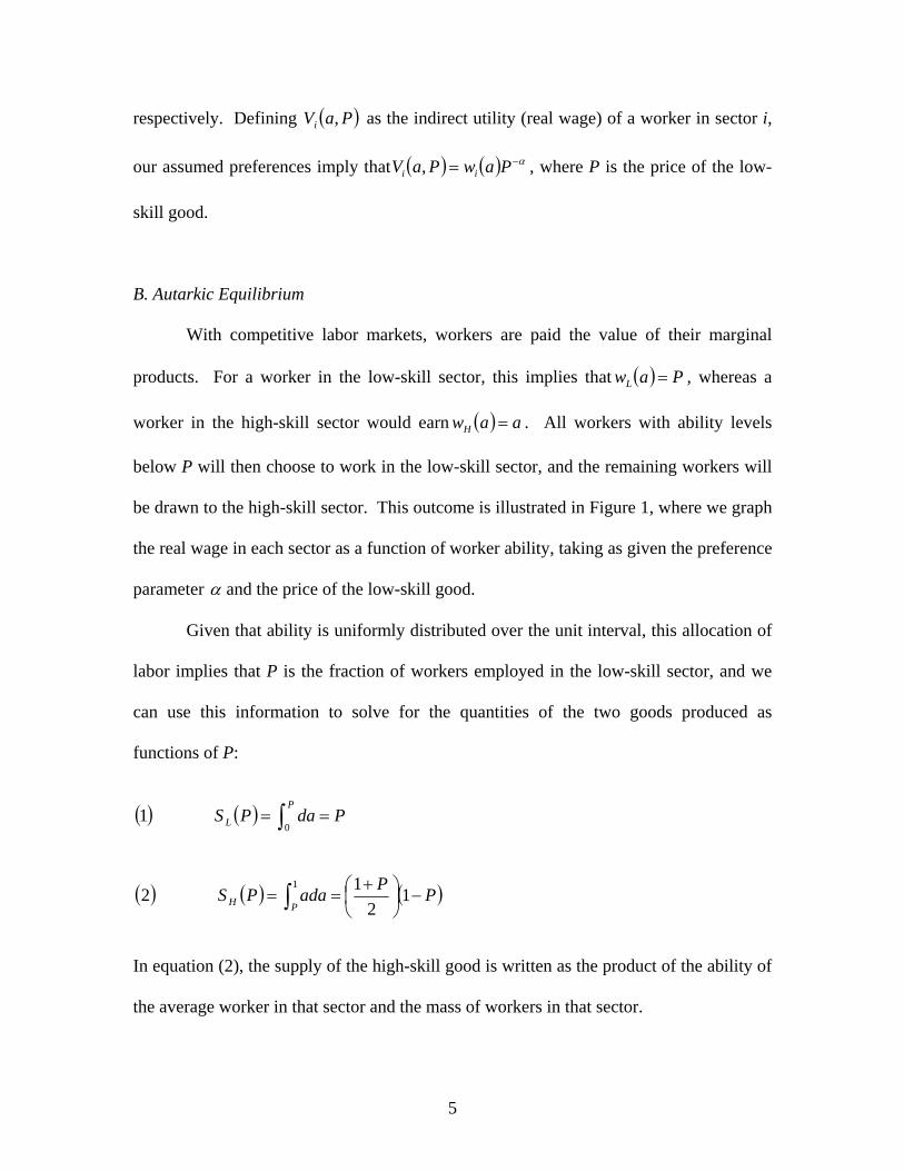
respectively. Defining ( )PaVi , as the indirect utility (real wage) of a worker in sector i,

our assumed preferences imply that ( ) ( ) α−= PawPaV ii , , where P is the price of the low-

skill good.

B. Autarkic Equilibrium

With competitive labor markets, workers are paid the value of their marginal

products. For a worker in the low-skill sector, this implies that ( ) PawL = , whereas a

worker in the high-skill sector would earn ( ) aawH = . All workers with ability levels

below P will then choose to work in the low-skill sector, and the remaining workers will

be drawn to the high-skill sector. This outcome is illustrated in Figure 1, where we graph

the real wage in each sector as a function of worker ability, taking as given the preference

parameter α and the price of the low-skill good.

Given that ability is uniformly distributed over the unit interval, this allocation of

labor implies that P is the fraction of workers employed in the low-skill sector, and we

can use this information to solve for the quantities of the two goods produced as

functions of P:

( ) ( ) PdaPSP

L == ∫ 01

( ) ( ) ( )PPadaPSPH −⎟

⎠⎞

⎜⎝⎛ +

== ∫ 12

121

In equation (2), the supply of the high-skill good is written as the product of the ability of

the average worker in that sector and the mass of workers in that sector.

6

Our assumption that all workers share the same Cobb-Douglas preferences

implies that the demands for the two goods are related in the following way:

( ) ( ) ( )LHL PDPPDα

α−

=1

3 .

In the absence of trade, the demand for each good must equal its supply. Using

( ) ( )31 − , this implies that the autarky price of the low-skill good is

( )α

α−

=2

4 AP .

Note that the uniform distribution of ability combined with the assumption of

Cobb-Douglas preferences implies that autarkic prices depend only on the single

preference parameter,α . When 1=α , consumers spend all of their income on the low-

skill good. As such, 1=AP and all workers choose to be employed in the low-skill

sector. At the other extreme, if 0=α there is no demand for the low-skill good and its

price is zero. In this case, all workers are drawn to the high-skill sector.

C. Trade

We now allow this country to trade with the rest of the world. We assume that

this is a small economy, taking the world price of the low-skill good as given. We are

particularly interested in the potential negative effects that trade might have on low-

income, displaced workers. As such, we focus our attention on the case where this

country has a comparative advantage in the high-skill good. Using TP to represent the

price of the low-skill good in world markets, we therefore restrict our attention to the case

where AT PP ≤ . From (4), this inequality can be re-written as

7

( )α

α−

≤2

5 TP .

We graph this inequality in Figure 2, which for future reference we divide into five areas.

The inequality in (5) is satisfied in areas B, C, D, or E in Figure 2. The inequality is

violated in area A, implying that the country would have a comparative advantage in the

low-skill good. Therefore area A is not relevant for the analysis in this paper.

The opening of trade creates three distinct groups of workers, which we illustrate

in Figure 3. Workers with APa ≥ choose to be in the high-skill sector in the absence of

trade and remain there once trade is opened. Liberalization clearly makes these workers

better off since the price index falls while their wage is unchanged. We refer to this

group of workers as “incumbents”. The area of trapezoid E measures the gross benefit of

trade (in real terms) that accrues to this group. Symmetrically, workers with TPa ≤

choose the low-skill sector in the absence of trade, and remain trapped in that sector once

liberalization occurs. Each worker in this group is clearly made worse off by trade since

their wage falls when measured in terms of either the low-skill or the high-skill good.

The area of rectangle B measures the magnitude of their loss. The remaining workers

choose to work in the low-skill sector in autarky, but move to the high-skill sector after

liberalization. We can refer to this group as “displaced,” in line with the terminology

used by Jacobsen, Lalonde, and Sullivan (1993), Lori Kletzer (2001) and others who have

attempted to measure the financial impact that globalization has had on this group of

workers. As illustrated in Figure 3, the lowest-ability displaced workers are worse off

after trade opens (their loss is measured by the area of triangle C), but those with the

highest ability are better off (their gain is measured by the value of triangle D).

8

D. Identifying the Median Voter

Given our assumption that ability is uniformly distributed, the median voter is the

worker for whom 5.0=a .4 Therefore the median voter is trapped in the low-skill sector

if AT PP ≤≤5.0 (area B in Figure 2), is displaced if AT PP << 5.0 (areas C and D in

Figure 2), and is an incumbent if 5.0≤≤ AT PP (area E in Figure 2).5 These areas are

labeled to correspond with the labeling in Figure 3.

3. Preferences Over Compensated and Uncompensated Trade

A. Preferences over Uncompensated Trade

Define a~ as the ability of a worker who is just indifferent between autarky and

uncompensated free trade. As Figure 3 illustrates, it must be the case that AT PaP << ~ ,

implying that there exists a displaced worker who is just indifferent between autarky and

free trade. By definition, a displaced worker is employed in the low-skill sector under

autarky and moves to the high-skill sector after liberalization. We can therefore find a~

by solving ( ) ( )THAL PaVPaV ,~,~ = for a~ . Doing so yields:

( ) αα −= 1~6 AT PPa

We are particularly interested in circumstances under which the median voter is

just indifferent between uncompensated trade and autarky. Therefore, we can set 5.0~ =a

4 Strictly speaking, this is true when there is no attempt at coupling redistributive policies with trade reform. In this case, the net welfare effect of trade is monotonically increasing in ability. As we show in Section 4, this monotonicity is not present when we allow for labor market policies that redistribute income. 5 From (4), this last inequality is satisfied for 4.0≤α . Depending upon our purposes, we can apply the same analysis to focus on any other voter, e.g., the 75th percentile voter, etc.

9

and then solve (6) for ( )αMP , the free trade price at which the median voter would be

indifferent between autarky and free trade, to obtain

( ) αα

α

ααα

211

221)7(

−

⎟⎠⎞

⎜⎝⎛

−⎟⎠⎞

⎜⎝⎛=MP .

From (7), ( ) ( ) 5.014.0 == MM PP and ( ) 5.0<αMP for 14.0 <<α . Using these

properties, we can deduce that when the median voter is a displaced worker, the graph of

equation (7) forms the boundary between areas C and D in Figure 2. The median voter

prefers autarky in area C, and prefers free trade (even in the absence of compensation) in

area D. Incumbents strictly benefit from uncompensated free trade if AT PP < . Therefore,

if 4.0<α the median voter is an incumbent and ( ) ( )αα AM PP = . The graph of this

relationship forms the boundary between areas A and E in Figure 2.

To recap, the majority of the workers would benefit from trade liberalization if the

combination of free trade prices and preferences lie in areas D or E in Figure 2. In

contrast, the majority would lose from trade liberalization if the relevant parameters lie in

areas B or C of that figure. It follows that a simple referendum on liberalization would

result in free trade in areas D or E and autarky in areas B and C. The existence of areas B

and C indicates that, as Mayer (1984) emphasized, free trade may not be the equilibrium

outcome when the median voter’s preferences determine trade policy.6

6 Our approach here is a bit different from Mayer’s. In his model agents have preferences over tariffs and he shows that the equilibrium tariff is the one preferred by the median voter. Since this tariff is zero only if the median voter’s factor ownership is identical to that of the economy as a whole, his result is that free trade in not likely to be the equilibrium outcome when agents vote on the level of protection. In contrast, we are assuming that prohibitive protection is already in place (so that the economy is effectively closed) and ask under what conditions society will choose to liberalize.

10

B. Alternative Compensation Schemes

Our focus in this paper is on analyzing compensation schemes that require the

government to have relatively minimal information. Essentially, we assume that the

government can only observe whether any particular worker is trapped, displaced, or is

an incumbent. Based upon this information, the government can either tax the worker or

offer a subsidy. Moreover, the subsidy can either depend upon the worker’s wage (and

therefore, in the case of the high-skill good, his ability) or it can be independent of the

worker’s wage.

Since we know that incumbents gain from trade, we assume that this group is

taxed, not subsidized. In fact, we assume something even stronger: we assume that it is

the incumbents who bear the full tax burden of any compensation program. Doing so

allows us to simplify the analysis considerably and it also captures the notion that in an

economy with a progressive tax system the wealthy (who, in our model, are incumbents)

pay they vast majority of the taxes. Let ( )TPG ,α represent the aggregate gross gain that

the incumbents receive in the move from autarky to trade. This is the maximum amount

by which the incumbents can be taxed and still prefer trade to autarky. We have:

( ) ( ) ( ) ( )

( ) ( )αα

α

−− −⎟⎠

⎞⎜⎝

⎛ +−=

−= ∫∫

ATA

A

P AP TT

PPP

P

daPaVdaPaVPGAA

21

1

,,,811

where ( )AP−1 represents the mass of incumbents, ⎟⎠⎞

⎜⎝⎛ +

21 AP represents the average

productivity (and therefore the average wage) of this group (measured in terms of the

11

numeraire good), and ( )αα −− − AT PP is the increase in real income due to the price

difference.

Let t be the marginal tax rate applied to the income of incumbents. Then total

(real) tax revenues equal ( )TPG ,α if

( )α−

⎟⎟⎠

⎞⎜⎜⎝

⎛=−

T

A

PP

t19 .

Who is compensated and how is the compensation paid? In principle, the

government could choose to compensate those trapped in the low-skill sector, displaced

workers, or both. For illustrative purposes, in this paper we focus on compensation

programs aimed at compensating the displaced workers. We do so primarily because the

vast majority of the public policy debate has focused on providing compensation for this

group7, but it should be clear that our analysis could be extended easily to consider the

implications of compensating those trapped in the low-tech sector.

Compensating displaced workers necessarily entails providing a subsidy to some

workers who already benefit from trade. Compensating this group also generates a

distortion as workers incorporate the promised compensation into their decisions

regarding where to work. For example, some workers who would make the efficient

decision to stay in the low-skill sector in the absence of compensation might be tempted

to move to the high-skill sector when the government subsidizes such movement. We

7 See, for example, Baily, Burtless, and Litan (1993), Jacobson, LaLonde and Sullivan (1993), Brander and Spencer (1994), Brecher and Choudhri (1994), Feenstra and Lewis (1994), Burtless, et al (1998), Parsons (2000), Hufbauer and Goodrich (2001), Kletzer (2001), and Kletzer and Litan (2001).

12

refer to these as “policy-induced” displaced workers in contrast to “trade-induced”

displaced workers.8

In earlier work (Davidson and Matusz 2002) we showed that the magnitude of the

distortion created by the compensation scheme depends upon the manner in which the

compensation scheme is tied to the worker’s wage. Suppose, for instance, that the

government implements a policy that fully compensates the marginal (trade) displaced

worker for his losses. From Figure 3, the identity of this worker is TPa = . This is also

the wage that he would earn (measured in terms of the numeraire) with free trade. The

compensation scheme that fully compensates this worker is either a wage subsidy ( )ω that

is the solution to (10) or an employment subsidy ( )ε that is the solution to (11), where in

both instances TPa = :9

( ) ( ) ( ) 1;,;,101

−=⇒=−

aPP

PaVPaV ATTHAL

αα

ωωω

( ) ( ) ( ) aPPPaVPaV ATTHAL −=⇒= −ααεεε 1;,;,11

where the indirect utility functions in (10) and (11) should be modified such that

( ) ( ) αεω −== 1;,;, PPaVPaV LL , ( ) ( ) αωω −+= PaPaVH 1;, , and ( ) ( ) αεε −+= PaPaVH ;, .

We compare the effects of the wage subsidy to that of the employment subsidy in

Figure 4.10 The broken line illustrates the indirect utility function for a high-skill worker

who receives a wage subsidy, whereas the indirect utility function for a high-skill worker

8 We recognize that decisions on the degree of openness constitute “policy” as well, but in this case we use the term “policy” to refer to the labor market policies that might be implemented to compensate workers for their losses. 9 With a wage subsidy, the worker’s subsidy-inclusive wage is ( )ω+1a . With the employment subsidy, his subsidy-inclusive wage is ε+a .

13

who receives an employment subsidy is illustrated by the solid line. In either case, an

efficient allocation of resources would entail only workers with [ ]AT PPa ,∈ moving to

the high-skill sector. With the wage subsidy, all workers with [ ]APaa ,ω∈ move, while

the employment subsidy induces all workers with [ ]APaa ,ε∈ to switch.11 The

deadweight loss in the former case is represented by the striped triangle. This is the

difference between the value of output of the low-skill good (measured at world prices)

that workers with [ ]TPaa ,ω∈ could produce and the value of output of the high-skill good

that these same workers actually produce. By analogy, we can calculate the deadweight

loss due to the employment subsidy. This magnitude of the deadweight loss in this case

is represented by the entire shaded triangle (both the striped and solid portions), and

therefore clearly exceeds the deadweight loss associated with the employment subsidy.

Despite the fact that the wage subsidy is preferable to the employment subsidy on

efficiency grounds, it is quite possible that the wage subsidy actually entails a larger

transfer from those who are taxed to those who are subsidized compared with an

“equivalent” employment subsidy. In this case, “equivalence” between the two

instruments means that a particular target worker is just as well off under either policy.

Consider again the case illustrated in Figure 4. The transfer involved with an

employment subsidy exceeds that for a wage subsidy when focusing only on policy-

displaced workers (i.e., those for whom ωε aaa ≤≤ ). There are two reasons for this.

First, more workers choose to switch sectors when an employment subsidy is offered;

10 To avoid clutter, we have not graphed the indirect utility function for a worker in the high-skill sector under autarky. 11 These two critical values are found by equating the subsidy-inclusive wage for a worker who moves to the high-skill sector with TP , the wage that the worker would earn in the low-skill sector. Doing so (and recognizing that these critical values must be non-negative) yields ( )εε −= TPa ,0max and ( )ωω += 1TPa .

14

therefore more workers are eligible for the program. Second, the employment subsidy

per worker exceeds the wage subsidy per worker because these workers have relatively

low ability, and therefore low wages. However, the transfer associated with the wage

subsidy is larger than that associated with the employment subsidy when we only

consider the trade-displaced workers. All inframarginal workers in this group have

higher ability (and therefore wages) than the marginal worker, and therefore compared

with the employment subsidy, the wage subsidy for each of them is larger in magnitude.

Clearly, as TP gets close to zero, the difference between the two policies in terms of the

transfer to the policy-induced displaced workers goes to zero, while the difference for the

trade-displaced workers goes to infinity.12 While not true for all parameter values,

numeric calculations show that indeed the transfer entailed by the wage subsidy is larger

than that associated with the employment subsidy over all relevant ranges, where we

describe the relevant ranges below. Therefore, in what follows, we assume that the

transfer is larger for the wage subsidy than it is for the employment subsidy.

4. Political Equilibrium

Suppose now that we start with a closed economy and consider a series of three

votes. The first vote is on whether or not to allow for free trade. In the event that the

majority votes against free trade, the process stops. If the vote is in favor of trade, the

second vote takes place on whether or not to provide compensation to displaced workers

for losses that they would incur due to liberalization. Here, we explicitly assume that any

compensation would be fully paid by taxing the incumbents (those who are in the high-

12 The maximum employment subsidy is finite, even if the marginal trade-displaced worker has zero ability. The wage subsidy, by contrast, goes to infinity as the free trade price goes to zero.

15

skill sector prior to reform) and received only by those who switch from the low-skill to

the high-skill sector subsequent to reform. We also assume that the amount of the

compensation is sufficient to fully offset the loss of the marginal trade-displaced worker.

If the result of this second vote is negative, the outcome is uncompensated free trade. If

the result is positive, the third vote is taken to determine whether the compensation

should be given in the form of a wage subsidy or an employment subsidy.

Our adoption of this particular structure induces a unique equilibrium despite the

multidimensionality of the problem. There is now a sizable literature on the way in

which political structures induce equilibrium.13 In the general context of policy

referenda, even as a reduced form for some broader political process, it seems unlikely

that governments are able to choose the structure of the voting agenda, and the particular

3-stage agenda we choose to focus on seems like a reasonable place to begin our analysis

of the impact of placing compensation on the political agenda. Nonetheless, the

possibility of having the government free to choose the agenda raises interesting

possibilities and we consider the case in which the government controls the agenda (i.e.,

the order of the votes). In solving this case we assume that the government’s goal is to

ensure free trade.14

Since we are only considering programs designed to compensate displaced

workers, it is clear that placing compensation on the agenda will not alter the political

outcome if the free trade prices and preference parameters fall in areas B or E of Figure 2.

In area B, the median voter is a trapped worker and this group is strong enough to block

any attempt to liberalize trade. In area E, the median voter is an incumbent and this

13 See Shepsle (1979) for the classic statement and Shepsle (1986) or Rosenthal (1990) for an overview.

16

group is strong enough to ensure that the equilibrium outcome will always be

uncompensated free trade. Thus, in what follows we focus attention on the areas in

which the median voter is displaced by liberalization (C and D).

To determine the equilibrium of this process, we begin with the third vote and

work backwards. For each vote, we assume that all agents vote unless they are

indifferent as to the outcome and that all agents vote sincerely15

As noted above, we assume that the magnitude of the transfer from the

incumbents to the displaced workers is higher for a wage subsidy than it is for an

employment subsidy. While this is not true for all parameter values, numeric techniques

show that it is true for all relevant parameter values.16 Given this assumption, all

incumbents prefer the employment subsidy to the wage subsidy. As argued above and is

evident from Figure 4, workers for whom [ ]TPaa ,ε∈ prefer the employment subsidy as

well. By contrast, all workers for whom [ ]AT PPa ,∈ prefer the wage subsidy. Finally,

workers for whom εaa < are indifferent between the two policies. They do not benefit

from either policy, nor do they bear the burden of the tax. Once again relying on our

assumption that ability is uniformly distributed, we conclude that the (more efficient)

wage subsidy will be chosen if and only if:

( ) ( ) ( ){ } ( ){ }TTATA PaPPPP ,112 ααα ε−+−>−

14 In a future paper we intend to consider alternative objective functions that the government might be attempting to maximize. 15 So, for example, if the trapped workers fail to block liberalization in stage 1, then they will choose not to vote in subsequent stages. This follows from the fact that they do not care whether or not compensation is offered (they do not get compensated nor do they have to pay for it) nor do the care about the type of compensation that may be offered. 16 In particular, this is true for all parameters where incumbents are unable to block any form of compensation due to their small share of the population. There does exist a range of parameters for which the employment subsidy is more costly to the incumbents, but for this range, the incumbents are sufficiently numerous that they can block all forms of compensation.

17

Holding TP constant, it is easy to show that the left hand side of (12) is increasing

in α while the right hand side is decreasing inα . That is, increasing α leads to a higher

proportion of trade-displaced workers who favor wage subsidies versus the group of

incumbents and policy-displaced workers who favor employment subsidies. Moreover,

holding α constant, decreasing TP increases the left-hand side of (12) while the right

hand side may either increase or decrease. Differentiation reveals, however, that even in

the case that the right hand side also increases, the increase is smaller in magnitude that

the increase in the left hand side. We conclude that lower values of TP also lead to a

higher proportion of trade-displaced workers relative to the coalition of incumbents and

policy-displaced workers. Putting both results together, wage subsidies will be selected

when a large share of income is spent on the low-skill good and when the free trade price

of that good is relatively low. Otherwise employment subsidies will be favored by a

majority of voters.

We now take a step back to examine the vote on whether there should be any

compensation at all. We assume that forward-looking voters rationally anticipate the

outcome of the third election. To start, we assume that they correctly anticipate that if a

majority votes in favor of compensation, they will ultimately choose wage subsidies.

Who will actively favor compensation? From Figure 4, wage subsidies will only benefit

workers for whom APaa ≤≤ω . Incumbents, who pay the taxes, will oppose

compensation. All remaining workers are indifferent. Note that for any set of parameters,

the mass of workers who favor compensation (knowing that the form of the

compensation will be a wage subsidy) is larger than the mass of workers who favor a

wage subsidy in the third vote. In addition, the mass of workers opposed to any form of

18

compensation is smaller than the mass of workers who favor employment subsidies in the

third vote. Since the larger group of incumbents and policy-induced workers is not

sufficiently large to obtain employment subsidies in the third vote, the smaller group

(consisting only of incumbents) is clearly too small to block compensation in the second

vote. Therefore, over the range of parameters where wage subsidies would prevail in the

third vote, a majority will favor compensation in the second vote.

Continue to think about the case where wage subsidies would be supported in the

third vote. Suppose we now move back to the first vote regarding the opening of trade.

Will liberalizers prevail? There are two cases to consider. In both cases, all trade-

displaced workers will clearly favor trade, since the worst that will happen is that they are

fully compensated for any loss. In fact, all trade-displaced workers will end up strictly

better off with trade compared with autarky. Even though policy-displaced workers

benefit ex-post from the compensation scheme, they are not fully compensated, and so

would oppose trade. Likewise, all workers who would remain trapped in the low-skill

sector oppose trade. Incumbents will support trade if the magnitude of the transfer

involved in the compensation scheme is not larger than the gross benefits that the group

receives from trade. Otherwise, this group will actually oppose free trade. In the latter

case, they rationally perceive that if trade is opened, they will ultimately be heavily taxed

to pay compensation to displaced workers. As we argued earlier, this possibility arises

when the free trade price of the low-skill good is very low, implying that the wage

subsidy necessary to compensate the marginal trade-displaced worker is very high.

We now take the other path, assuming that an employment subsidy would be

chosen in the third vote. The analysis of the second vote is similar in this case, but there

19

are some differences. In this case, we recognize that the group favoring an employment

subsidy is larger than the group favoring a wage subsidy. However, some workers who

are allied with the incumbents during the third vote are on the other side in the second

vote. In particular, the group favoring compensation in the second round includes

workers with ability ωε aaa ≤≤ . If the third round vote is close, this difference is

significant enough that the result can be a majority voting for compensation in round two

when they correctly forecast an employment subsidy in round three. However, it may be

that incumbents are numerous enough that they can essentially get what they want

without help from other quarters, meaning that they can on their own defeat any move to

implement compensation in round two. This would be true if the preference parameter is

sufficiently small (suggesting that ( )αAP is small and the mass of incumbents is large).

If the preference parameter is not too small, incumbents cannot block

compensation. When the vote for trade liberalization is held, all trade-displaced workers

and all incumbents vote in favor, while all others vote against.17 If the preference

parameter is sufficiently small, no compensation will be forthcoming, and the only group

supporting free trade will be the incumbents. All others will be opposed.

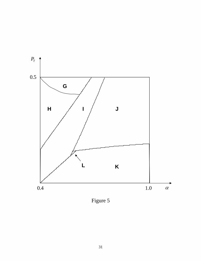
Putting all of the pieces together results in Figure 5, which was drawn by

numerically calculating the boundaries of the various inequalities discussed in this

section. Each of the areas in this figure corresponds to the different outcomes of the

sequence of votes. Before describing the areas individually, we reiterate that, holding the

free trade price of the low-skill good constant, the mass of incumbents and policy-

displaced workers falls relative to the mass of trade-displaced workers as the preference

20

parameter gets larger. That is, moving from left to right in this diagram, trade-displaced

workers become relatively more numerous and incumbents become relatively less

numerous. Similarly, moving from top to bottom (holding the preference parameter

constant and reducing the free trade price of the low-skill good), trade displaced workers

become more numerous relative to incumbents.

We start with area G, which is a subset of area C from Figure 2. For this set of

parameters, no trade will be the political outcome because the median voter loses from

trade and will not receive compensation. The reason is that for this set of parameters, the

incumbents are strong enough to block all compensation. Knowing this, the displaced

workers who are harmed by liberalization align themselves with the trapped workers to

block free trade. This is one case, however, where the government could manipulate the

agenda to change the outcome. Free trade can be achieved by moving the vote on

compensation up to stage 1. The incumbents, looking ahead, will now realize that if they

vote down compensation in stage 1, liberalization will be voted down in the next stage.

Thus, they shift their support, vote for compensation and team with all displaced workers

to push through liberalization in stage 2. This turns out to be the only case in which

changing the agenda can alter the outcome.

If parameters lie in area H (which is a subset of area D in Figure 2), then the

outcome will be uncompensated free trade. Here, incumbents are strong enough to block

all compensation and the median voter is a displaced worker who gains from trade even

in the absence of compensation. Although the displaced workers would prefer additional

compensation, they do not have enough power to push it through on their own.

17 In the case of an employment subsidy, numeric calculations indicate that the magnitude of the transfer is always smaller than the gross benefits of trade accruing to the incumbents.

21

In area I, incumbents are not strong enough to block all compensation, but they

are strong enough to obtain the form of compensation that they find least costly (the

employment subsidy). Since trade-displaced workers benefit, they ally with incumbents

to successfully obtain free trade.

Areas J, K, and L represent the parameter space where the incumbents are not

strong enough to block compensation, and not even strong enough to obtain the least

costly form of compensation. In these areas, the result of the vote in round three will be a

wage subsidy. Moreover, in areas L and K, the magnitude of the transfer involved in the

wage subsidy is larger than the magnitude of the gross benefits of trade, so incumbents

will actually oppose trade in the first round, though they support trade if parameters lie in

area J. In areas J and K, supporters of free trade outnumber opponents. But in area L,

opposition by incumbents is sufficiently strong that, when allied with those trapped in the

low-skill sector and the policy-displaced workers, they are able to block trade. It is

important to note that in this case, unlike area G, changing the agenda will not alter the

outcome. No trade is the outcome in area L regardless of the order of the votes.

Does the opportunity to provide compensation lead to a higher probability of trade

reform? That depends. Our analysis shows that allowing for the possibility of

compensating trade-displaced workers does lead to trade in instances where trade would

have otherwise been blocked, but conversely, there are situations where trade is blocked

that would have otherwise been permitted (area L). This situation arises when the cost of

compensating the displaced workers is relatively high, causing the incumbents to alter

their stage 1 behavior and vote against freer trade.

22

5. Conclusions

We see this paper as making three contributions. First, we illustrate a simple,

tractable model of agent heterogeneity that has a variety of uses in analyzing the

economics and political economy of trade. Second, we have extended the standard

referendum model of political economy of trade policy to incorporate compensation; and

third, our specific application considered the issue of whether compensation can “save

free trade”.

For many issues of current interest in trade theory and policy, worker

heterogeneity is of considerable importance. When such heterogeneity is central,

standard trade models in which agents own only one factor of production are less helpful,

and expanding the number of factors to permit, say, multiple qualities of labor expands

the dimensionality of these models in unhelpful ways. The continuum assumption has

proven to be exceptionally useful in disciplining exactly this sort of dimensionality

problem in a wide range of applications in economics from Aumann’s (1964) use of the

continuum in demonstrating the identity between the core and the set of Walrasian

equilbiria, to Dornbusch, Fisher and Samuelson’s (1977) continuum model of a Ricardian

economy with many goods. Of particular relevance for our work in this paper is Mayer’s

(1984) use of the continuum in a median voter model of trade policy-making. Mayer’s

model involves agents with one unit of labor and some non-negative quantity of capital

so that agents’ capital-labor ratios are distributed continuously. Standard results from

endogenous tariff theory yield a determinate relationship between agent endowment and

preference over the tariff (a one-dimensional issue in a two-good model). Since this

preference varies continuously with endowment, Mayer is able to use simple Reimann

23

integration to identify the median voter. In our case, it is ability that varies continuously,

but our analytic approach is very similar. In addition to the ease of political economic

analysis, however, we would first like to stress the usefulness of the continuum for the

analysis of worker heterogeneity in a simple general equilibrium context. As the first

substantive part of the paper indicates, we are able to provide a simple, but compelling,

analysis of the impact of trade on labor market outcomes in a model with worker

heterogeneity. The graphical illustration of this model also indicates its pedagogical

value.

Our second contribution involves the extension of a Mayer-type referendum

model to endogenize the compensation, as well as the trade policy, decision. Although

there is a sizable literature on the common-sense notion that compensation, in addition to

moving a potentially Pareto-improving policy in the direction of an actual Pareto

improvement, increases the political sustainability of trade liberalization, there is very

little in the way of systematic political economic analysis on this question. Early work by

Harry Johnson and Rachel McCulloch (1973) argued that a welfare maximizing

government that was politically constrained to offer protection might gain relative to a

tariff by using the distribution of quota revenues to support lower levels of protection.

Bhagwati and Feenstra (1982) apply similar reasoning in a model in which a welfare

maximizing government uses tariff revenues to induce lower levels of lobbying on the

part of a protection-seeking labor union. While Bhagwati and Feenstra do present an

explicit model of political-economic interaction, the assumption of a welfare-maximizing

government seems broadly inconsistent with the underlying goals of political economic

analysis. More closely related to our work is a recent paper by Christopher Magee

24

(2003). As with Bhagwati and Feenstra, in Magee’s model the government is an active

player, but unlike Bhagwati and Feenstra, instead of seeking purely to maximize welfare

the government is of the Grossman-Helpman (1994) sort. Contrary to Bhagwati and

Feenstra, Magee finds that, precisely because it lowers the cost of any given level of

protection, the presence of compensation permits the government to offer more

protection.18 In particular, at low levels of protection (such as those currently applied in

virtually all industrial countries) compensation may hinder further liberalization.19

There are two major differences between Magee’s analysis and ours. First, where

Magee’s analysis evaluates the contribution of compensation to liberalization at the

margin, our analysis focuses on the contribution of compensation to the overall

sustainability of liberalization. That is, our model considers a choice between fixed,

finite policy options. Second, and perhaps more importantly, Magee’s analysis, like

Bhagwati and Feenstra’s, is really only indirectly about liberalization. As in Grossman

and Helpman, what is really for sale is protection. In our analysis the issue on the agenda

is liberalization. We think it is worth noting that trade policy in the post Second World

War era has been overwhelmingly about liberalization, and that arguments about

compensation have been directly related to this policy and not to protection per se.

Furthermore, this commitment to liberalization has been only very indirectly related to

the sorts of forces modeled in standard work on political economy (Nelson, 2003). Thus,

while the details of inter-sectoral variation in protection may be well-modeled in

18 This effect is particularly large in Magee’s simulations because he takes the “result” of Golberg and Maggi (1999) that the government’s weight on aggregate social welfare is 50 to 70 times the weight placed on contributions. 19 This result is contrary to that obtained by Fung and Staiger (1986) who analyze compensation in a model without domestic political competition. Their model treats domestic compensation as part of the international political economy of trade policy. In their paper the implicit bribe is not directed to domestic factors of production but to one’s negotiating partners in a trade agreement.

25

something like a Grossman-Helpman framework, we believe that the issue of overall

sustainability of a liberalization policy (adopted for some unmodeled reason) is more

clearly treated in a framework such as that developed here.

Directly related to the last comment, our third contribution is an evaluation of

claims that a well-constructed compensation program can help “save free trade”

(Lawrence and Litan, 1986). As we noted in the introduction, there is both good and bad

news here. In the context of our simple model we find that allowing for the possibility of

compensating trade-displaced workers does lead to trade in instances where trade would

have otherwise been blocked, but conversely, there are situations where trade is blocked

that would have otherwise been permitted.

Our analysis suggests that this framework is potentially very useful and we think

that all three contributions could usefully be extended. With respect to the basic model of

the economy: in its current form, it would be useful to formulate the core theorems of

trade theory for this model; and, more generally, since this is a general equilibrium model

with worker heterogeneity, it would be interesting to permit type (i.e. ability) to be

private information and to introduce labor market institutions to deal with that

heterogeneity (e.g. efficiency wages, etc.). With respect to the political economy model:

first, it would be interesting to consider alternative structures of referendum; second,

introducing an active government with alternative objectives would seem to be a useful

extension; and third, it would seem important to consider the sustainability of

compensation in the context of less robust information than considered here. Finally,

with respect to the specific issue of “saving free trade”, it would be interesting to bring

more concrete structure to the analysis to permit some more specific evaluation of the

26

role of compensation (i.e., with respect to the model, what part of the parameter space do

we find ourselves in?).

27

( ) α−×= AAAL PPPaV ,

( ) α−×= AAH PaPaV ,

aAP

Figure 1

28

A B

C

TP

0.1

5.0

0.1 α

D E

4.0

Figure 2

29

( )AL PaV ,

( )AH PaV ,

aAP 0.1

( )TH PaV ,

( )TL PaV ,B C

D E

TP a~

Figure 3

30

aAP

( )TH PaV ,

( )TL PaV ,

TP

( )ε;, TH PaV

( )ω;, TH PaV

εaωa

Figure 4

( )AL PaV ,

31

G

H I J

K

α

TP

5.0

4.0 0.1

L

Figure 5

32

References

Aumann, Robert (1964). “Markets with a Continuum of Traders”. Econometrica; V.32-

#1/2, pp. 39-50.

Baily, Martin Neil, Gary Burtless, and Robert Litan (1993). Growth with Equity.

Washington D.C.: Brookings Institution.

Brander, James and Barbara Spencer (1994). “Trade Adjustment Assistance: Welfare and

Incentive Effects of Payments to Displaced Workers.” Journal of International

Economics, V.36: 239-261.

Brecher, Richard and Ehsan Choudhri (1994). “Pareto Gains from Trade, Reconsidered:

Compensating for Jobs Lost.” Journal of International Economics, V36: 223-238.

Burtless, Gary, Robert Lawrence, Robert Litan, and Robert Shapiro (1998).

Globaphobia: Confronting Fears about Open Trade. Washington D.C.:

Brookings Institution.

Davidson, Carl and Steven J. Matusz (2002). “Trade Liberalization and Compensation.”

Michigan State University Working Paper.

(2004). International Trade and Labor Markets: Theory, Evidence and

Policy Implications. Kalamazoo: W.E. Upjohn Institute.

Dixit, Avinash and Victor Norman (1986). “Gains from Trade without Lump-Sum

Compensation.” Journal of International Economics, V.21-#1/2, pp. 111- 122.

Dornbusch, Rudiger, Stanley Fisher, and Paul Samuelson (1977). “Comparative

Advantage, Trade and Payments in a Ricardian Model with a Continuum of

Goods”. American Economic Review; V.67-#5, pp. 823-839.

33

Feenstra, Robert and Jagdish Bhagwati (1982). “Tariff Seeking and the Efficient Tariff”.

In Jagdish Bhagwati, ed. Import Competition and Response. Chicago: University

of Chicago Press/NBER, pp. 245-258.

Feenstra, Robert and Tracey Lewis (1994). “Trade Adjustment Assistance and Pareto

Gains from Trade.” Journal of International Economics, V.36: 201-222.

Fung, K.C. and Robert Staiger (1996). “Trade Liberalization and Trade Adjustment

Assistance”. In Matthew Canzoneri, Wilfred Ethier, and Bittorio Grilli, eds. The

New Transatlantic Economy. Cambridge: Cambridge University Press/CEPR, pp.

265-286.

Goldberg, Pinelopi and Giovanni Maggi (1999). “Protection for Sale: An Empirical

Investigation”. American Economic Review; V.89-#5, pp. 1135-1155.

Grossman, Gene and Elhanan Helpman (1994). “Protection for Sale”. American

Economic Review; V.84-#4, pp. 833-850.

Guesnerie, Roger (2001). “Second Best Redistributive Policies: The Case of International

Trade”. Journal of Public Economic Theory; V.3-#1, pp. 15-25.

Hammond, Peter and Jaume Sempere (1995). “Limits to the Potential Gains from Trade”.

Economic Journal; V.105-#432, pp. 1180-1204.

Hufbauer, Gary and Ben Goodrich (2001). “Steel: Big Problems, Better Solutions.”

Policy Brief. Washington D.C.: Institute for International Economics.

Jacobson, Louis, Robert LaLonde, and Daniel Sullivan (1993). “Earnings Losses of

Displaced Workers.” American Economic Review, V.83: 685-709.

Johnson, Harry G. and Rachel McCulloch (1973). “A Note on Proportionally Distributed

Quotas”. American Economic Review; V.63-#4, pp. 726-732.

34

Kemp, Murray and Henry Wan (1986). “Gains from Trade with and without

Compensation”. Journal of International Economics; V.21-#1/2, pp. 99-110.

Kletzer, Lori (2001). What are the Costs of Job Loss From Import-Competing

Industries? Washington D.C.: Institute for International Economics.

Kletzer, Lori and Robert Litan (2001). “A Prescription to Relieve Worker Anxiety.”

Policy Brief No. 73. Washington D.C.: Brookings Institution.

Lawrence, Robert and Robert Litan (1986). Saving Free Trade: A Pragmatic Approach.

Washington D.C.: Brookings Institution.

Mayer, Wolfgang (1984). “Endogenous Tariff Formation”. American Economic Review;

V.74-#5, pp. 970-985.

Magee, Christopher (2003). “Endogenous Tariffs and Trade Adjustment Assistance”.

Journal of International Economics; V.60-#1, pp. 203-222.

Nelson, Douglas (2003). “Political Economy Problems in the Analysis of Trade Policy”.

Inaugural Lecture, University of Nottingham.

Parsons, Donald (2000). "Wage Insurance: A Policy Review." Research in Employment

Policy, V.2: 119-140.

Rosenthal, Howard (1990). “The Setter Model”. in J. Enelow and M. Hinich, eds.

Advances in the Spatial Theory of Voting. Cambridge: CUP, pp. 199-234.

Shepsle, Kenneth (1979). “Institutional Arrangements and Equilibrium in

Multidimensional Voting Models”. American Journal of Political Science; V.23:

27-58.

(1986). “The Positive Theory of Legislative Institutions: An Enrichment

of Social Choice and Spatial Theory”. Public Choice; V.50: 135-178.

35

Spector, David (2001). “Is It Possible to Redistribute the Gains from Trade Using Income

Taxation?”. Journal of International Economics; V.55-#2, pp. 441-460.