Embed Size (px)
Citation preview

Can analysts pick stocks for the long-run?
Forthcoming, Journal of Financial Economics
Oya Altınkılıça, Robert S. Hansenb,*, Liyu Yeb
aSchool of Business, George Washington University, Washington, D.C. 20052, USA bA.B. Freeman School of Business, Tulane University, New Orleans, LA 70118, USA
c U.S. Treasury, Fannie Mae, Washington D.C., 20016, USA
Abstract
This paper examines post-revision return drift, or PRD, following analysts’ revisions of their stock recommendations. PRD refers to the finding that the analysts’ recommendation changes predict future long-term returns in the same direction as the change (i.e., upgrades are followed by positive returns, and downgrades are followed by negative returns). During the high-frequency algorithmic trading period of 2003-2010, average PRD is no longer significantly different from zero. The new findings agree with improved market efficiency after declines in real trading cost inefficiencies. They are consistent with a reduced information production role for analysts in the supercomputer era. JEL classification: G02, G14, G24.
Keywords: Analysts’ forecasts, Financial analysts, Financial markets, Investment banking, Market efficiency, Security analysts, Behavioral finance. First draft: January, 2010 Latest draft: February, 2015 We thank the editor, Bill Schwert. We thank an anonymous referee for very constructive comments, and for helpful comments received on early drafts of the paper we thank colleagues at The Freeman School of Business, Tulane University and The School of Business at George Washington University. * Corresponding author contact information: Tulane University, New Orleans, LA 70118. Tel +504-865-5624. E-mail addresses: [email protected] (O. Altınkılıç), [email protected] (R.S. Hansen), [email protected] (L. Ye).

1
1. Introduction
For decades researchers have examined average long-run stock returns after sell-side security analysts
revise their recommendations for buying and selling stocks. The universal finding is that the
recommendation changes predict future long-term returns in the same direction as the change (i.e.,
upgrades are followed by positive returns, and downgrades are followed by negative returns). This
phenomenon is known as post-revision return drift (PRD). This result has supported the hypothesis that
PRD persists because investors typically underreact to analysts, responding partly at their revision
announcements and slowly thereafter, perhaps taking months. It has also underpinned the nested
hypothesis that security analysts are better-informed, skilful at information discovery from non-public
sources (e.g., from insiders) and from neglected public information in inefficient markets, as noted by
Grossman and Stiglitz (1980).1
This article provides new evidence about PRD that extends the literature in a number of ways. The
primary contribution is the finding that average PRD is no longer persistently different from zero in the
May 2003 through 2010 sample post-period. A second contribution is new results that show a causal
relationship between analysts’ revisions and PRD is not supported in many tests of the PRD cross-section.
A third contribution is new evidence from the PRD cross-section regarding the investor underreaction
hypothesis and the informed analyst hypothesis. Results from tests for underreaction that use proxies
suggested by other researchers do not support the underreaction hypothesis in the post-period. For
instance, one finding in this article shows there is no significant association between PRD and analysts’
coverage, a widely used proxy for underreaction. Tests of the informed analyst hypothesis that employ
proxies for better-informed analysts used in prior research, do not support the idea that analysts typically
supply new information that correctly picks stocks for the long run. One example is that the PRD cross-
1 Givoly and Lakonishok (1979), Womack (1996), Hong, Lim, and Stein (2000), Gleason and Lee (2003), Jegadeesh, Kim, Krische, and Lee (2004), and Loh (2010) discuss underreaction to analysts.

2
section reveals no significant association with extreme revisions, a commonly used proxy for better-
informed analysts.
A further contribution of this article is new findings supporting the alternative explanation for the
persistence of PRD noted by Barber, McNichols, and Trueman (2001), that transaction costs, a real
inefficiency, are high enough to fence PRD from profitable arbitrage trading strategies. The results agree
with the explanation that PRD has broadly vanished due to a general decline in transaction costs, pushed
down to historic lows by decimalization, the expanded use of supercomputers, and algorithmic trading.
The PRD disappearance coincides with notable reductions in transaction costs that have attracted profit-
taking arbitrageurs to PRD.2
The empirical findings in this article are robust to a number of concerns. First, the bad model concern
is addressed by using PRD measures built with different asset pricing models and benchmark returns,
including the market return and the return on a similar group of stocks identified by the four
characteristics model return of Daniel, Grinblatt, Titman, and Wermers (1997). Using these same models
to estimate returns in both the post-period and the sample pre-period, 1997 through April 2003, suggests
that the insignificance of the average PRD in the post-period is unlikely to be the result of switching
expected return models. Still, the findings do not preclude that future research could yield expected return
models that capture long-run drift effects. Second, the findings are not the result of a particular method
for aligning the measurement of the PRD. Third, the conclusions are reinforced for refined types of
revisions noted in the literature, which include consensus recommendations and extreme revisions. Lastly,
out-of-sample tests confirm a general absence of PRD in the post-period. This tests uses international
2 In the supercomputer era the equity trading market was transformed into the supercomputer intermediated market (Angel, Harris, and Spatt 2012). Along with decimalization that cuts the bid-ask spread increments to 1¢ per share from 6.25¢ (a 16th of a dollar), supercomputers cut electronic transaction costs, institutional commissions, and arbitrage costs to historic lows, enabling high frequency trading (hundreds and thousands of buy and sell transactions per minute) using complex algorithmic models and software at low cost, fueling growth in hedge funds and trading volume, as well as attenuation of some anomalies (Korajczyk and Sadka, 2004; French, 2008; Chordia, Roll, and Subrahmanyam 2011; Chordia, Subrahmanyam, and Tong 2014; Hendershott, Jones, and Menkveld 2011; Beneish, Lee, and Nichols 2013).

3
analysts’ revisions in the other Group of 7 countries: Canada, France, Germany, Italy, Japan, and the UK.3
The findings show that drift after analysts’ revisions in these countries also is not informative in the post-
period, supporting similar findings for U.S. analysts.
PRD is examined from several perspectives, reflecting different ways that researchers have measured
PRD, and a variety of samples that are employed for different tests. One PRD measure uses an event
study approach in which the revisions are aligned on their announcement date, similar to that used by
Womack (1996) and by Jegadeesh, Kim, Krische, and Lee (2004). This measure is examined in the Event-
Time Sample (see Appendix A.1 for sample descriptions). A second measure evaluates PRD from a
portfolio perspective in calendar time and examines the returns on buy portfolios of upgraded stocks and
sell portfolios of downgraded stocks, and compares their differences. This drift measure is similar to that
employed in Barber, McNichols, and Trueman (2001) and utilizes the Portfolio Sample. PRD is examined
from a third viewpoint first introduced in this article, which aligns firms on their earnings report
announcement dates, and compares the drift for firms with upgrades to the drift for the other firms with
continuations (i.e., those with unchanged recommendations), and similarly for the downgrades. This
method controls for the influence of post-earnings announcement drift (PEAD) and uses the Earnings
Sample. Revisions in each of these three Samples are examined in both the post-period and in the pre-
period. This provides opportunities to replicate findings from the earlier studies, and to compare the pre-
and post-period PRD behavior side-by-side. PRD is also examined in a sample of consensus
recommendations within each period.4
Although average transaction costs are lower in the post-period, it is unlikely that they have entirely
disappeared (for example, see Beneish, Lee, and Nichols 2013; Boehmer, and Wu, 2013). Under the
transaction cost rationale, some PRD is likely present for stocks with relatively high transaction costs. In
3 We thank the referee for suggesting this out of sample test. 4 Dimson and Marsh (1984), Elton, Gruber, and Grossman (1986), Stickel (1992), and Mikhail, Walther, and Willis
(2004) also study PRD. Cowles (1933, 1944) does not find evidence of PRD in a much earlier sample period.

4
agreement, after sorting the Event-Time Sample into trading volume deciles, some statistically significant
average PRD exists in the lowest decile, or 10% of the revisions. Significant average PRD is also present
in the lowest deciles in sorts by firm size and by analysts’ coverage of the firm. The VSC revisions which
are common to the lowest deciles for all three characteristics, and make up 3% of all revisions, are
expected to have high transaction costs. In agreement VSC revision stocks have a number of
characteristics that are consistent with high transaction costs. Their stock prices are among the lowest, so
trading a certain weight of these shares in a given portfolio will be more costly (i.e., requiring the sale of
many more shares). They are twice as likely to be listed on the Nasdaq, where bid-ask spreads are larger
than for NYSE-listed firms in the post-period (Angel, Harris, and Spatt 2012). Furthermore, VSC revision
stocks are among the smallest firms, with other firms’ average equity valued 50 times higher. Also, their
trading volume is the lowest, showing they are in limited short-run demand and supply.
The findings also allow that some PRD could be the unintended result of the way in which the long-
run abnormal returns are measured. For example, the small sample evidence of PRD is ever-present in the
lowest deciles in a number of sorts for the Event-Time Sample, while the evidence is inconsistent in the
lowest deciles of the Portfolio and Earnings Samples.
While PRD may come from analysts’ new information discovery and asset pricing model effects, this
article documents a third potential source: drift that is associated with other recent news and events about
the covered firm. A number of studies find that analysts often piggyback their reports on recent events
and news, which contribute to magnifying return reactions measured during the days around the revision
announcements, and to masking how much of the return reaction can be credited to analysts’ new
information (Altınkılıç and Hansen, 2009; Altınkılıç, Balashov, and Hansen 2013; Kim and Song, 2014).
Similarly, recent events and news themselves can be associated with their own return drift which could
confound the average PRD and consequently raise the question of how much of the PRD can be credited
to analysts’ revisions. This issue is addressed in this article through examination of concurrent event drift
from the notable reported earnings event using the Earnings Sample, which allows for control of the well-

5
known post-earnings announcement drift (PEAD) that could enlarge measures of average PRD. The new
findings using the Earnings Sample reveal that after controlling for PEAD, the PRD contains little
incremental information that can be credited to analysts in the post-period, confirming the third source of
drift.5
The new findings contribute to research related to analysts’ performance in the market for new
information in their role as information intermediaries. The results show that, on average, analysts’
revisions are not highly correlated with subsequent long-run returns, indicating that analysts do not
provide new information that is relevant for the long-run for typical investors. Analysts face greater
competition in the market for new information in the post-period, as lower transaction costs have enabled
arbitrageurs to quickly harvest more mispricing opportunities, shrinking the potential pool of neglected
information. Therefore, to the extent that analysts’ supply of new information is derived from their
discovery of neglected public information, in the post-period they are confronted with greater scarcity of
such information. The heightened competition for neglected information would seem to imply that
analysts may now allocate less of their time and effort producing such new information.6
The new findings should also be relevant for researchers interested in market efficiency. Jensen (1978)
suggests that markets are efficient as long as economic agents cannot profit from the analysts’
information. Fama (1970) notes that markets are efficient as long as agents cannot reliably predict long
run common stock returns. The findings from the post-period support both definitions of market
efficiency. The general decline in transaction costs has allowed information to be incorporated more
quickly and completely into security prices, eliminating both profit opportunities from strategies that use
5 Barber, McNichols, and Trueman (2001) note that PRD could also be an anomaly. 6 Analysts’ sources for new information have also likely been reduced by reforms that limit their access to non-
public information. Such reforms and rules enacted in the pre-period include the Global Settlement, NASD Rule 2711, and Regulation Fair Disclosure. Still, the reforms’ impact is likely to be mixed, so some analysts may not be barred from some sources of non-public information in the post-period. For example, analysts’ access to information from informed parties through school-ties declined following the reforms (Cohen, Frazzini, and Malloy 2010), while they continue to have access to some non-public information from firm management through conference hostings (Green, Jame, Markov, and Subasi 2014). The reforms could contribute to lower transaction costs by reducing information asymmetry (Eleswarapu, Thompson, and Venkataraman 2004).

6
analysts’ revisions, as well as the predictability of long-run returns based on the revisions. The
disappearance of PRD therefore exemplifies how rational pricing of securities interacts with changes in
real inefficiencies to extend market efficiency.
One alternative explanation for the lack of significant PRD in the post-period, which conserves the
view that analysts supply ample new information, is that investors no longer underreact to new
information from analysts’ revision announcements. Perhaps the profound economic forces of the
supercomputer era, which greatly accelerated trading frequency at minimal cost, also elevated investor
attention to all stocks, thereby significantly expanding investor awareness and hastening their reaction to
news that affects stocks’ prices. An important implication of this increased awareness theory, if the
revisions supply analysts’ new information, is that announcements of analysts’ revisions should be met
quickly with widespread investor reaction that quickly impounds most of the new information, if not all,
into stock prices. Thus, in the post-period, the average return reaction to revision announcements should
contain economically significant evidence of analysts’ new information, all else the same. However, this
implication is not supported by recent studies, which report that that the announcement period price
reaction to analysts’ reports contains little new information that can be attributed to the analysts
themselves (Altınkılıç and Hansen, 2009; Loh and Stulz, 2011; Altınkılıç, Balashov, and Hansen 2013).
The findings in this article widen the empirical evidence indicating little average investor reaction to
analysts’ reports.
The remainder of the article proceeds as follows; Section 2 describes the sample; Section 3 examines
PRD in side-by-side comparisons of the post-period and the pre-period; Section 4 examines evidence of
PRD in the 3% sample of the Event-Time Sample revisions; Section 5 examines the underreaction
hypothesis and the informed analyst hypothesis; Section 6 examines PRD in a sample of international
stocks; the article concludes with final thoughts and implications for future research in Section 7.

7
2. Sample description
The samples used in this article draw from real time or no source code needed recommendation
revisions from First Call Historical Database (FCHD) from 1997 through 2010 (batch recommendations,
initiations, and resumptions are excluded), which have the control variables used in this study as
identified from the literature. Recommendation levels range from 1 to 5 respectively: strong buy, buy,
hold, sell, and strong sell. If the new recommendation level is lower (higher) than the previous
recommendation level, it is an upgrade (downgrade). Recommendations issued after 4 PM are taken as
issued the next trading day. If one brokerage issues multiple recommendations on the same day for the
same company, only the latest is retained. If there are multiple upgrades (downgrades) for the same
company on the same day, the upgrade (downgrade) is counted only once. Conflicting revisions for the
same stock on the same day and on stocks with no earnings announcement in the prior year are deleted.
CRSP provides daily stock prices and volume. Industry classifications are from Ken French’s website.
[Insert Table 1 about here]
Revision annual frequency is usually higher over 2005-2007 for both upgrades and downgrades.
Covered firms and brokerage firms in the sample follow a similar pattern (Table 1).
3. Post-revision return drift
The first measure of PRD is in revision event-time, using the long-term average abnormal buy and
hold returns aligned on the third trading day after the revision announcement day. Measuring drift starting
three days after the announcement avoids return shocks from confounding events immediately around the
revision announcement. Initially, PRD is calculated two ways that use different asset pricing models: the
Market Model, denoted MM, and the characteristics model of Daniel, Grinblatt, Titman, and Wermers
(1997), denoted DGTW. The sample for these estimations is the Event-Time Sample.

8
The drift for firm i, with a duration of d trading days that starts three trading days after the
recommendation announcement, denoted , , is firm i’s raw return during the duration period, , ,
less that period’s return from the asset pricing model, ;
, , ∏ 1 , ∏ 1 (1)
where denotes the or measures (see Appendix A.2 for variable definitions). For Market
Model returns, is the CRSP value weighted market index return. For characteristic adjusted returns,
is the return on the characteristics’ portfolio of firms matched on market equity, market-to-book,
and on prior one-year return quintiles. In both cases, reported durations include 20, 60, and 120 trading
days.
3.1. The graphical view
Figure 1 Panel A displays the post-period average PRD for the full 120-day for the Event-Time
Sample. MM PRD after upgrades are announced is generally flat, while it is modestly positive after the
downgrades. The DGTW PRD measure is negative over the 120-day after downgrades and even more so
after upgrades. Thus, for both measures, the average PRD behavior is mixed: sometimes it agrees with the
revisions, thus agreeing with the informed analyst thesis, and sometimes it is contrary to the revisions.
[Insert Figure 1 about here]
In the pre-period, the average PRD behavior is also mixed (Figure 1, Panel B). PRD is positive after
the upgrades under either asset pricing model, which agrees with the informed analyst view. For
downgrades, however, rather than being negative, the PRD is positive, using either asset pricing model.
This is contrary to the behavior anticipated when following the advice of informed analysts’ revisions.
The irregular PRD behavior clearly shows that revisions do not reliably foretell future long-term
return behavior, on average.

9
[Insert Figure 2 about here]
A further evaluation of the return performance uses a measure that is conditioned on the direction of
analysts’ revisions; called the “up-less-down” strategy, which seeks to capture the difference between
PRD after upgrades and PRD after downgrades. In effect, this is a strategy that invests long in the
upgraded stocks and short in the downgraded stocks, providing a gross assessment of the return from
analysts’ information. Note the up-less-down measure is not capable of evaluating expected profits; that is
the gross value from the entire investment strategy net of the likely transaction costs from executing the
strategy. When the gross value from this up-less-down strategy is significantly positive, the average PRD
only reveals that the recommendations have behaved, in combination, as if they are informative for the
investment duration.
For the post-period, the up-less-down MM PRD generally is slightly negative over the 120-day after
the revisions are announced, and so is the DGTW PRD (Figure 2, Panel A). This does not agree with the
informed analyst view. In contrast, in the pre-period the strategy yields positive PRD for both drift
measures, which does not agree with the informed analyst view. While this positive drift resembles
qualitatively similar findings from prior studies in earlier sample periods, the only source for this positive
up-less-down drift in Figure 2 is the long upgrade leg of the portfolio, because the short downgrade leg
earns negative returns (Figure 1). In other words, a strategy of going long stocks after both upgrades and
downgrades, contrary to the strategy that strictly follows analysts’ advice, would have earned a higher
return than the up-less-down strategy. The PRDs computed using value-weighted returns are not
materially different from the equally weighted case reported in Figures 1 and 2 (unreported).
3.2. The decline of PRD
This section documents in more detail the behavior of PRD in the post-period and in the pre-period.

10
3.2.1. The Event-Time Sample
[Insert Table 2 about here]
Consider first the univariate regression of PRD on the revision upgrade indicator variable, UP, that is
one if the recommendation is an upgrade and zero if it is a downgrade. The regression equation is thus
, , (2)
where registers the additional drift that is associated with analysts’ upgrades relative to their
downgrades.
In the post-period the regression estimate shows the MM measure of PRD is positive over the first
20 days after day 3, although the coefficient estimates are not economically large at around 27-28 bp
(with significance at the 5% level). The two longer duration drifts are not significant, diminishing in
magnitude or turning negative (Table 2, Panel A). Qualitatively similar results are recorded for the DGTW
PRD (Table 2, Panel A).
In contrast, the pre-period upgrade average PRD is significantly positive relative to the downgrade
PRD, at all durations, typically at the 1% level, for both the MM and the DGTW measures. Moreover, the
magnitude of the UP coefficient estimates for the pre-period are often large, over five times larger than
the estimates for the post-period. The findings from the pre-period agree with the informed analyst
hypothesis and are qualitatively similar to findings reported in earlier studies.
[Insert Table 2 about here]
The second regression model is a multivariate specification that includes twelve exogenous binary
variables that control for several other effects affecting the return behavior, similar to the measure
employed by Jegadeesh, Kim, Krische, and Lee (2004)
, ∑ , , (3)

11
where for firm i the right-hand side includes UP and twelve exogenous binary variables, : Retp, Ret2p,
Frev, SUE, BP, and EP are 1 if the control variable is above the sample median, and Turn, Size, LTG, SG,
TA, and Capex are 1 if the control variable is below the sample median. Otherwise, each binary variable
takes a value of zero.
Higher momentum stocks are expected to receive more favorable revisions, to the extent that analysts
rely on momentum from prior earnings to generate their revisions. Lee and Swamanathan (2000) show
that drift is inversely related to prior trading volume. Basu (1977) reports that high earnings-to-price
multiple firms outperformed other firms. Fama and French (1992) report that subsequent returns for high
book-to-price ratio (BP) firms outperform others. Lakonishok, Shleifer, and Vishny (1994) show that drift
underperforms following high average long-term growth in sales, and La Porta (1996) shows that
underperformance follows high forecasted earnings growth. Authors have also reported that drift is
greater for small firms (Banz, 1981). Sloan (1996) reports that more negative accruals are associated with
higher drift. In contrast, Chan, Chan, Jegadeesh, and Lakonishok (2001) report that higher accruals often
support higher accounts receivable and inventory, in support of greater sales. Beneish, Lee, and Nichols
(2001) report that high capital expenditures are typically followed by lower drift.
The estimates for the incremental impact of UP on PRD in the multivariate regression are similar to
the estimates in the univariate regression (Table 2, Panels A and B). In the post-period, the informed
analyst hypothesis is supported in only one case, the 20-day duration drift, and is not significant in the
longer durations. In contrast, in the pre-period the incremental PRD associated with UP is significantly
positive for all three durations, for both the MM and DGTW measures of PRD, consistent with the
informed analyst hypothesis.
Additional post-period tests that exclude revisions during the financial crisis period (September 2008
through the sample period end), provide results that are qualitatively similar to the full sample results
(Table 2, Panel C).

12
3.2.2. Portfolio Sample
The next measure of PRD uses a calendar portfolio approach, similar to Barber, Lehavy, and
Trueman (2007), and focuses on three portfolio classes: the Buy portfolio of all upgraded stocks, the Sell
portfolio of all downgraded stocks, and the Buy-less-Sell portfolio, which is the difference between the
upgraded and downgraded stocks. This sample is the Portfolio Sample.
Portfolio drift is measured using the Carhart (1997) extension of the Fama and French (1992)
expected returns model,
(4)
where for date t the dependent variable is the return on a portfolio j of recommendations less the risk-free
rate, and the right-hand side variables are respectively: the return on the value-weighted market index less
the risk-free rate; the return on a portfolio of small-cap stocks less the return on a portfolio of large-cap
stocks; the return on a portfolio of high book-to-market value stocks less the return on a portfolio of low
book-to-market value stocks; and the return on a portfolio of recent high return stocks (winners) less the
return on a portfolio of low recent return stocks (losers). The factors and the risk-free interest rate are
collected from Ken French’s website.
The expected signs of the coefficients in equation (4) are: small cap and small value portfolios
respectively have higher expected returns than the large cap and growth portfolios. The holding period
returns are measured over the 60 trading days starting on day three after the revision announcement. Drift
performance is measured by the intercept estimate, , in equation (4). The estimation results are reported
in Table 3.
[Insert Table 3 about here]
In the post-period, estimates for both the Buy portfolio and the Sell portfolio indicate no significant
causation between the revisions and PRD. Similarly, Buy-less-Sell portfolio PRD is not significant (Table
3, Panel A). Neither result is expected by the informed analyst view
13
In the pre-period the Buy portfolio drift estimate is positive and statistically significant, in agreement
with the informed analyst hypothesis and some prior studies (Table 3, Panel B). However, the Sell
portfolio estimate indicates no significant post-revision return drift, which is inconsistent with the view
that downgrades anticipate lower prices in the future. The Buy-less-Sell portfolio PRD remains
significant, however, registering the strong relative performance of the Buy portfolio.
Results from further tests in the post-period, after removing revisions issued during the financial crisis
period (September 2008 through the sample period end), are weaker than the full post-period results
(Table 3, Panel C), as none of the portfolios’ PRD is significant.
3.2.3. The Earnings Sample
Thus far, the tests follow the custom of comparing PRD after all upgrades with PRD after all
downgrades. However, these tests overlook the possible external influence in those revisions when
analysts’ decisions to upgrade or downgrade their revisions rely at least in part on publicly known factors
that in and of themselves have some power to predict future drift. To the extent that analysts piggyback
their revisions on drift predictors in this way, there may be a revision selection bias that could be
influential enough to cause spurious agreement between the revisions and subsequent PRD, even when
the analyst is not communicating new information. An important example taken up here is piggybacking
the revisions on known predictors of PEAD, an enduring long-run drift anomaly (e.g., see Fama, 1998).
For example, by upgrading (downgrading) after good (bad) earnings surprises, the revision could
associate with subsequent positive (negative) PEAD, independent of any new information the analysts
might deliver in the revision announcement. While some control for this bias is possible in the Event-
Time Sample tests by including unexpected earnings (SUE) among the right-hand side factors in the PRD
regression estimations, spurious correlation could still be operative that biases the revision PRD to agree
with the informed analyst view, even though analysts may only be tracking PEAD alone, not seeking to
offer new information.

14
To address this selection bias concern, further PRD tests use the Earnings Sample, which contains all
quarterly earnings announcement events from FCHD, where each announcement enters the sample once
regardless of the frequency of analysts’ revisions. Within this sample the relevant upgrade revisions and
the downgrade revisions are identified from the Event-Time Sample. By construction, all other
observations have no recommendation revision and are called continuations.
The Earnings Sample therefore permits testing if PRD after upgrades and after downgrades, where
both are associated with earnings announcements, differs from the drift for all continuations that are
likewise associated with earnings announcements.
In the Earnings Sample, drift for the continuations is measured starting on the third trading day after
the earnings announcement. Thus, this drift after the firm’s concurrent earnings announcement is PEAD,
and it contains no drift that is attributable to a revision. Drift after each recommendation revision is also
measured starting on the third trading day after the earnings announcement. By construction, the post-
revision drift for the revisions includes the drift from the concurrent earnings announcement, PEAD, plus
the incremental drift that is created as a result of new information released by the analyst’s revision
announcement.
To estimate the incremental drift impacts from the revisions relative to the drift from the earnings
news, the upgrades, downgrades, and continuations are pooled in a single regression that includes two
dummy variables; UP equals one for the upgrades and DOWN equals one for the downgrades, in addition
to the twelve factors. The estimated regression is thus
, ∑ , , (5)
Regression (5) therefore tests if revisions produce incremental drift beyond what could be associated
with the concurrent PEAD. If upgrades produce significant additional drift, then is expected to be
positive. Likewise, if downgrades create more negative drift beyond the PEAD, is expected to be
negative.

15
[Insert Table 4 about here]
In the post-period the average upgrade increment to PRD is not statistically significantly positive, for
any of the three durations of the MM PRD measure (Table 4, Panel A). Similarly, for the downgrades the
average increment to PRD is not statistically significantly negative, for any duration, for the MM PRD
and DGTW PRD measures (Table 4, Panel A). These findings are not consistent with the informed analyst
hypothesis. In light of these findings, it is plausible that evidence of significant PRD reported in the post-
period Event-Time Sample could contain bias to the extent that revisions piggyback on predictors of
future drift that are not fully reflected in the twelve factors.
In the pre-period, by contrast, the PRD for the upgrades is significantly positive, for both MM PRD
and the DGTW PRD, for all three durations (Table 4, Panel B). For the downgrades, half of the DOWN
coefficient estimates are significantly negative. Some of these findings agree with the informed analyst
thesis, and are qualitatively similar to findings that are reported in prior studies whose sample period
overlaps the pre-period.
For the post-period, further tests are conducted after removing observations during the financial crisis
period (September 2008 through the sample period end). These estimates are never significant,
qualitatively similar to the full post-period results (Table 4, Panel C).
Hereafter, because the reported post-period findings are not altered qualitatively by excluding crisis
period revisions, to conserve space only results for the whole post-period sample are reported.
3.2.4. The Matched-Earnings Sample
One concern is that by including all earnings announcements, the Earnings Sample tests might not
adequately control for the extent to which firms associated with analysts’ revisions differ from other firms
associated with continuations, in ways that are not controlled by the regression model despite the
inclusion the twelve factors. For example, perhaps PRD is not linear in some of the factors, or perhaps
there are measurement concerns, like the fact that the inclusion of a momentum measure among the

16
independent variables might not adequately control spurious correlation that could be attributed to
earnings announcement news.
Further tests, therefore, use the Matched-Earnings Sample. In the Matched-Earnings Sample, each
upgrade and each downgrade from the Earnings Sample is matched to a similar continuation in the
Earnings Sample, where similarity is determined using the Propensity Score method. Thus, a Probit
model is first estimated for the Earnings Sample using the set of twelve predictor variables to obtain
propensity scores for all revisions and continuations. The Matched Earnings Sample consequently
consists of all upgrades and downgrades and their respective matched continuations using the closest
Propensity Score. In the Matched-Earnings Sample the measured drift for the revisions includes PEAD in
addition to the incremental PRD triggered by the informativeness of the analysts’ revisions. The
continuations, however, contain only PEAD and no incremental information effects from revisions (as in
equation 5).7
[Insert Table 5 about here]
For the Matched-Earnings Sample, Panel A of Table 5 reports mean values for the twelve factors
used to estimate the Propensity Scores, for the upgrades and their corresponding matched continuations,
and likewise for the downgrades. The factor means show the Propensity Score identifies matched
continuation firms that are similar to the firms, in terms of the twelve factors.
7 The Propensity Score matching test is common in financial settings, including underreaction events, where
selection bias is a concern. Lee and Wahal (2004) look at IPO underpricing and venture capital reputation; Drucker
and Puri (2005) examine SEOs by the firm’s lending bank; Lee and Masulis (2010) look at underwriter and venture
capitalist reputations and the firm’s earnings management. For further discussion of the tests, see Heckman (1979),
Heckman and Robb (1986), Heckman, Ichimura, and Todd (1997, 1998), and Roberts and Whited (2012).

17
If analysts’ revisions are informative for the long-run, there should be a significant difference between
the revision firms’ average PRD and the matched firms’ average PRD, all else the same: positive between
the estimated coefficients for UP and UPmatched, and negative between the estimated coefficients for
DOWN and DOWNmatched.
In the post-period, there is positive drift measured by the MM PRD for both the upgrades and the
upgrade matched firms. However, the difference between their PRD is not statistically significant (Table
5, Panel B), in each duration, for both the MM PRD and the DGTW PRD. The lack of a significant
difference between the drift after the revisions and the drift after the continuations, points to drift
observed after the revisions reflecting drift from concurrent earnings announcements, rather than from
underreaction to analysts’ information.
In the pre-period significantly positive PRD is common for the UP revisions and their matched
continuations, but the evidence indicating the two differ is weak for both asset pricing models, except in
the 3 month duration. The findings are mixed for downgrades, as there is both significantly positive and
significantly negative drift, which is not anticipated by the informed analyst hypothesis.
Most of the empirical results from the post-period Earnings Sample and the Matched Earnings Sample
provide no consistent pattern of significant PRD from analysts’ revisions, but some do. Similarly, in the
pre-period, a pattern of significant PRD difference is typically uncommon.
To summarize the univariate and multivariate PRD cross-section findings reported in Tables 2-5, these
tests reveal in the post-period that PRD, measured using methods reported in earlier research, is not
economically meaningful and often it does not agree with the direction in which analysts have revised
their stock recommendations. While the significant PRD for the 20-day duration in the Event-Time
Sample is aligned with the informed analyst hypothesis, in that Sample the evidence is generally mixed.
Moreover, the finding does not appear to be robust in the other Samples. In the Portfolio and Earnings
Samples there is no significant average PRD that agrees with the informed analyst hypothesis. Similarly,
18
in the Matched Earnings Sample there is no significant difference between average PRD for upgrades and
their matches, or downgrades and their matches, across all three drift durations.
In the pre-period Event-Time Sample, the cross-section regression estimates show upgrades have
statistically significant impact on PRD. This is confirmed with the Buy-less-Sell findings in the Portfolio
Sample, as well as the UP findings and 3-month duration DOWN findings in the Earnings Sample. There
is also support for this conclusion among the mixed results using the Matched Earnings Sample,
Propensity Score tests. A number of these pre-period results also agree with findings reported in earlier
studies.
4. Has post-revision return drift totally disappeared?
If PRD persists because of high transaction costs, then economically significant PRD could still exist
in post-period sub-samples that are more likely to have relatively high transaction costs, even if the
average PRD is not significant. This section reports results from several tests that are designed to
determine if average PRD within sub-sample deciles is significant when the revision firm characteristics
suggest large transaction costs are likely to be present. The tests focus on three characteristics: Volume,
Firm Size, and Coverage.
4.1. Volume
Everything else the same, low volume firms are likely to have higher costs of illiquidity than other
firms, raising their trading cost (Amihud, 2002). To the extent that low volume indicates limited supply of
stock at current prices, transaction costs are likely to be even higher when the trading strategies include
shorting downgraded stocks.
Trading Volume in the firm’s shares is measured by the average daily trading volume over the prior
calendar year. For the post-period, in the Event-Time Sample, PRD is insignificant in most trading
Volume deciles, however it is distinctly present in the lowest decile using either drift measure, across all

19
three durations (Table 6, Panel A). This agrees with the transaction cost thesis, to the extent that the
lowest Volume decile stocks typically have relatively larger costs. In contrast, for the Portfolio Sample,
significant PRD is not consistently present in the lowest decile (Table 6, Panel B); negative PRD is
present in the lowest Sell portfolio decile, but significant PRD does not occur in the lowest deciles for the
Buy, or the Buy-less-Sell portfolios (Table 6, Panel B). Also, for the Earnings Sample, there is little
evidence of significant PRD across durations for the upgrades (Table 6, Panel C), while for the
downgrades (Table 6, Panel D), there is evidence in the lowest decile only for the 20-day duration.
[Insert Table 6 about here]
By contrast, in the pre-period Event-Time Sample, significant drift is broadly apparent up and down
the Volume deciles. For example, in seven of the 20-day deciles, for both MM and DGTW, PRD is
noticeably strong statistically in the lowest deciles across all three durations and both drift measures
(Table 6, Panel A). Under the transaction costs thesis, this pattern of significant average PRD over most
deciles would suggest relatively high transaction costs range across far more revisions in the pre-period.
In the Portfolio Sample deciles, PRD is significant in eight Buy deciles, two Sell deciles, and eight Buy-
less-Sell deciles (Table 6, Panel B). In the Earnings Sample, PRD is present in three deciles for most
durations, while no obvious cluster pattern is present. For upgrades, PRD is evident in the lowest decile
across the two estimation methods (Table 6, Panel C). The evidence is mixed in higher Volume deciles; in
some cases it is statistically significant, but in one of those cases there is a wrong sign for the
underreaction view (Table 6, Panel D).
4.2. Firm size
Firm size is also a relevant characteristic of trading costs, which are likely to be high for smaller
firms. For example, Hendershott, Jones, and Menkveld (2011) find that while quoted and effective bid-

20
ask spreads are significantly narrower in the supercomputer era, that outcome is weakest for the small
firms.
In post-period sorts by Firm Size, measured by the logarithm of equity size at the fourth quarter end
of the last fiscal year, the UP coefficient in the Event-Time Sample is distinctly statistically significant in
the lowest decile, for each duration and both estimation methods (Table 7, Panel A). Lowest decile
impacts are also present in the Portfolio Sample for the Buy and Buy-less-Sell portfolio, but not for the
Sell portfolio (Table 7, Panel B). In the Earnings Sample, the PRD evidence is weaker; the UP coefficient
is not significant in the lowest decile for any asset pricing model and any duration, and the DOWN
coefficient in the lowest decile is significant at the 5% level for the 20-day duration (Table 7, Panels C
and D).
[Insert Table 7 about here]
In the pre-period Event-Time Sample, PRD is present in several firm size deciles, including the lowest
(Table 7, Panel A). In the Portfolio Sample, PRD is apparent in the lower three Buy portfolio deciles
(Table 7, Panel B), which is enough to make the Buy-less-Sell portfolio drift significant. The Sell
portfolio drift, however, shows little economic significance. In the Earnings Sample, PRD is significant in
some mid-level deciles for the upgrades, but not in the lowest or in the highest deciles. For the
downgrades, PRD is significant for most durations in the lowest decile, and in a few other deciles up and
down the firm size chain.
4.3. Analyst Coverage
Average PRD is next examined in deciles after sorting by Coverage, the number of recommendations
issued for the firm over the prior calendar year. Studies suggest that analysts’ coverage could impact the
firm’s trading costs. For example, Kelly and Ljungqvist (2012) report that coverage reduces information

21
asymmetry, thereby lowering the bid-ask spread. Chen, Harford, and Lin (2014) report coverage increases
monitoring of managers, reducing agency costs that also could impact trading costs.
In the post-period Event-Time Sample, there is again a distinct pattern of significant PRD in the lowest
coverage decile, for both estimation methods and all three durations (Table 8, Panel A). In the other
deciles, PRD is not significantly greater than zero, for both drift measures and all durations. The Portfolio
Sample again shows asymmetric evidence of PRD in the lowest Buy decile. The results are significant for
the Buy portfolio at the 5% level, insignificant in the lowest Sell portfolio decile, and significant in the
lowest Buy-less-Sell portfolio decile. For the Earnings Sample 20-day drift is significant for the upgrades
for both measures, but not for the longer durations (Table 8, Panel C). PRD also has a weaker presence in
the lowest decile for the downgrades (Table 8, Panel D).
[Insert Table 8 about here]
The pre-period PRD is significant in many of the bottom five Coverage deciles and in other higher
deciles in the Event-Time Sample (Table 8, Panel A). It is also evident in the Portfolio Sample across the
Buy deciles, and the Buy-less-Sell deciles (Table 8, Panel B). The Earnings Sample similarly shows
significant drift across the lower two deciles for the upgrades and the downgrades, though not widely
across the lowest decile. Otherwise, some deciles show significant PRD in the direction of the revision, at
varying levels of significance with no basic pattern (Table 8, Panels C and D).
4.4. VCS revisions
To further identify the nature of the revisions associated with the post-period PRD in some of the
above sorts, the revisions in the lowest decile in sorts of each of the three characteristics are examined to
determine how well these revisions account for the average PRD in the lowest respective decile in the
sorts of the two other characteristics.

22
For the post-period Event-Time Sample, removing the lowest Volume decile revisions eliminates
significant PRD in the lowest decile for both Firm Size and Coverage (Table 9, Panel A). Removing the
lowest Firm Size decile revisions makes PRD in the lowest Volume decile insignificant for all three
durations, and eliminates PRD in many but not all Coverage deciles (i.e., not 20 day) where significant
drift remains drift at the 5% level (Table 9, Panel B). Dropping the lowest Coverage decile revisions also
wipes out significant PRD in the lowest Volume and Firm Size deciles (Table 9, Panel C).
[Insert Table 9 about here]
This one-by-one comparison of the individual characteristics shows the lowest Volume decile revisions
appear to account more effectively for the PRD: There is greater comparative loss of statistical
significance of the remaining drift for the other two characteristics. Also, the removal of the lowest
Volume decile revisions pushes down the remaining average drift in the other lower deciles more than
does the removal of Firm Size or Coverage (Table 9, Panels A-C).
However, it is unlikely that all of the small sample post-period PRD can be credited to just one of the
three characteristics. To further identify this PRD, the influence of the revisions that are common in each
of the lowest deciles in separate sorts of each characteristic is examined (Volume, Size, and Coverage;
hereafter VSC revisions). VSC revisions are a small sample, making up 3% of all revisions.
Removing the VSC revisions from the sample eliminates significant PRD in the lowest Volume decile
and in the lowest Firm Size decile (Table 9, Panel D).
Under the transaction cost rationale for the PRD persistence, the VSC revision should have
characteristics that are associated with high transaction costs. The VSC revision stocks are far less liquid,
as the average non-VSC revision firm size is over 50 times larger in average market value of equity, and
22 times larger in terms of shares outstanding (Table 10, Panel A). The VSC revision firms have lower
average stock price; their post-period mean price of $15.70 is less than half of the post-period mean price
of $33.40 for the non-VSC revision firms. Furthermore, twice as many VSC revision firms are Nasdaq-
23
listed than non-VSC revision firms. Angel, Harris, and Spatt (2012) note median quoted bid-ask spreads
are larger in the supercomputer era for Nasdaq-listed firms than for NYSE-listed firms. Also, average
coverage for the typical VSC revision firm is very low, at 1.75 analysts, versus 10 for the typical non-VSC
revision firm. Also, the VSC revisions’ sub-sample is small, consisting of only 3% of all revisions.
[Insert Table 10 about here]
The low analyst interest in these firms could mean they expect to find little information with enough
value to cover transaction costs, even though the average PRD is high relative to all firms. The
characteristics also point to possible asset-pricing concerns. For example, the VSC revision characteristics
include being among the smallest of firms, which have well-known asset pricing issues (see Banz, 1988;
Fama and French, 1992; Fama, 1998).
The general evaluation for the post-period based on Tables 6-10 is that PRD, on average, does not play
an important role. Across the three characteristics of Volume, Firm Size, and Coverage in all three
Samples (Tables 6-8), excluding the lowest decile, average PRD is insignificant in the other bottom five
deciles for all three durations for both the MM and DGTW measures. The lowest decile evidence is mixed:
in the Event-Time Sample average PRD is significant for all durations and both drift measures. However,
in the Portfolio Sample average PRD in the lowest decile is inconsistent, and in the Earnings Sample it is
insignificant except for DOWN in the 20-day duration decile. In the higher deciles for each of the
characteristics average PRD is rarely statistically significant, and at times is significant but in the opposite
direction anticipated by the underreaction and informed analyst hypotheses. Further study of the VSC
revisions that are common to lowest deciles for each of the three characteristics (Tables 9 and 10), support
the understanding that their average PRD is largely accounted for by small samples of 10% and 3% of the
revisions that have characteristics that typify higher transaction costs. The results further show that this
significant average PRD tends to be limited to the Event-Time Sample, as it is not common in the

24
Portfolio and Earnings Samples. One interpretation is that, in the supercomputer era, much of the PRD
has been driven away by arbitrageurs.
In contrast, in reviewing the pre-period findings, average PRD is significant across many of the lowest
five deciles and across all three holding period durations in the Event-Time Sample, for both the Buy and
the Buy-less-Sell portfolios in the Portfolio Sample, as well as almost half the cases for the Earnings
Sample. Significant average PRD is present in many higher deciles, for all durations in the three Samples.
This shows the economic magnitude of the average PRD is greater in the pre-period than in the post-
period. One interpretation is that high transaction costs are common across a range of revisions.
5. Are underreaction and informed analysts associated with significant PRD?
Although many findings in the post-period show that significant long-run drift is less common after
revisions, except for the small sub-sample of high transaction costs stocks, the evidence still may not be
enough to rule out that stock prices underreact to analysts’ new information. In particular, underreaction
could create drift in sub-samples of the PRD cross-section. Sub-samples could also contain evidence of
analysts’ ability to identify new information for the long-run. This section reports results from further
testing for significant investor underreaction and better-informed analysts.
5.1. Underreaction tests
The underreaction hypothesis tests of the PRD cross-section use two proxies for investor
underreaction that have been suggested in the literature: share turnover and analyst coverage.
5.1.1. Share turnover
Studies suggest stock prices tend to react more slowly to new information for low turnover stocks
(i.e., those with low fractions of shares traded), as their investors are inclined to pay less attention to the
stocks, all else the same. Thus, when new information about these firms is made public, that information

25
is incorporated in the stock price more slowly, resulting in underreaction to the news, ceteris paribus. For
example, Bhushan (1989) reports that when a firm announces earnings, there is greater underreaction over
time to both good and bad earnings news for the stocks with lower turnover, hence greater PEAD in
absolute value (see also Barber and Odean, 2008; and Loh, 2010). Given this underreaction behavior,
when revisions release analysts’ new information, greater average underreaction is expected for the
lowest turnover stocks, ceteris paribus. Upgrades will be associated with more positive drift and
downgrades with more negative drift, in the respective lowest turnover deciles. Turnover does not predict
PRD should be found higher deciles, where investor reaction to new information is expected to be swift.
Test results are reported for the Event-Time, Portfolio, and Earnings Samples.
In the post-period Event-Time Sample, PRD is statistically significantly positive and large for firms in
the lowest turnover decile for all three durations, and for 20-day PRD in the second lowest decile, for both
the MM and the DGTW drift measures (Table 11, Panel A). Farther up the turnover decile chain, irregular
drift is present in a few deciles-sometimes significantly large positive, sometimes significantly large
negative, and mostly neither. After removing the lowest Volume revisions from the Event-Time Sample,
no significant PRD is present in any turnover decile (Table 11, Panel B). Qualitatively similar results are
found when the smaller sample of VSC revisions are removed. The lack of significant PRD after
removing these revisions indicates underreaction cannot be widespread. Mixed findings are evident for
the Portfolio Sample: Buy portfolio drift is high and significant in the lowest turnover decile but not for
the Sell portfolio. The evidence of underreaction for the Buy-less-Sell portfolio is inconsistent and weak.
Indications of underreaction are also weak in the Earnings Sample (Table 11, Panel C and D). For
example, in the lowest five UP deciles average PRD is not significant in any of the deciles. Relative to
continuations, there is no significant drift in the lowest five DOWN deciles, except for the 120-day MM
PRD measure.
[Insert Table 11 about here]

26
While some of the lowest turnover cell evidence agrees with the underreaction prediction, the broader
pattern from the turnover findings across the Samples is not reconciled by underreaction (Table 11, Panel
C).
In the pre-period Event-Time Sample, significantly large 20-day PRD is common in almost every
turnover decile, in a number of lower deciles, and in even more upper deciles, across all three durations
(Table 11, Panel A). Thus, there is no standout pattern of significant PRD in the lowest deciles versus
others, as expected by significant underreaction alone. Sufficient transaction costs could exist across the
deciles that could account for much of the drift. In the Portfolio Sample, PRD in the lower Buy (Sell)
decile portfolios is significantly positive (negative), while the upper three deciles also have significantly
positive PRD (Table 11, Panel C). The Buy-less-Sell portfolio has significant drift in the lowest and the
highest deciles. These irregular patterns are not explained by the underreaction hypothesis. For the
Earnings Sample, there is no evidence of significant PRD in the lowest turnover deciles for the upgrades.
Except for the lone case for 120 day, there is also no significant PRD for the lowest decile for downgrades
(Table 11, Panels D and E).
5.1.2. Analysts’ coverage
A second proxy for underreaction is analysts’ coverage of the recommended stock. Authors suggest
that when the stock has low coverage, information flows more slowly across investors and moves rapidly
for the widely covered stocks. For example, Brennan, Jegadeesh, and Swaminathan (1993) report prices
react slower to common information for less covered stocks. Hong, Lim, and Stein (2000) find positive
drift when coverage is lower. Zhang (2008) reports greater underreaction by analysts themselves to
earnings news for firms that have lower coverage. This understanding therefore predicts that greater drift
should be evident for firms with the lowest analyst coverage, all else the same.
As reported earlier (Section 4.3), in the Event-Time Sample post-period significant PRD is present in
the lowest Coverage decile but not in higher deciles (Table 10). However, the opposite result is found in

27
the Portfolio Sample, as significant PRD is not present in the lowest four deciles, but is present in two of
the highest three deciles. In the Earnings Sample the lowest decile evidence is weak.
In the pre-period, significant PRD exists in a number of deciles across the three Samples, after sorting
by Coverage (Tables 6, 7, and 8). However, this evidence is mixed and its irregular patterns do not
consistently agree with the hypothesis that underreaction is significant in the lowest decile and not in
higher deciles.
5.2. Informed analyst hypothesis
A second test for evidence of underreaction in the PRD cross-section focuses on the nested hypothesis
that in the first place requires that analysts possess new information that they will release with their
revisions. While a number of results thus far show PRD is not regularly connected with analysts’ new
information, the hypothesis could still be relevant in sub-samples of the PRD cross-section. Further tests
therefore focus on the nested informed analyst hypothesis, using four different proxies for better informed
analysts that are reported by researchers.
5.2.1. Extreme revisions
Researchers find that analysts’ extreme revisions tend to release more fresh information, on average
(Stickle, 1995; Womack, 1996; Boni and Womack 2006; Green 2006; Kecskes, Michaely, and Womack
2013). A revision to strong buy or to strong sell thus signals the typical analyst’s strongest endorsement
for buying or selling the stock. One test of the informed analyst hypothesis therefore examines the impact
of six dichotomous extreme revision variables on the PRD, in the multivariate drift regression: UPtoSB
for the upgrades to strong buy, UPtoB for the upgrades to buy, UP for all other upgrades, DOWNtoS for
those downgrades to Sell, and DOWNtoSS for the downgrades to strong sell.
[Insert Table 12 about here]

28
In the post-period the extreme revisions are not generally associated with unusual PRD. For the MM
PRD measures, one of the 18 upgrade dummies (to UP) indicates a positive revision impact (significant at
the 10% level), and two of the 18 downgrade dummy estimates (both to DOWN) show the revision impact
is associated with a contradictory positive impact (Table 12, Panel A).
In contrast, in the pre-period a few of the extreme upgrades have statistically significant positive
impacts on the drift, which is more evident for the DGTW method (Table 12, Panel B). For downgrades
the results are weaker, as only two extreme downward revisions have a significantly negative impact and
two have a significantly contrary positive impact.
5.2.2. Brokerage reputation
The second proxy for informed analysts is the brokerage firm’s reputation in the securities market.
Authors report that more prestigious brokerage firm analysts are better informed (Stickel, 1992; Fang and
Yasuda, 2013; Kecskes, Michaely, and Womack 2013). To the extent that underreaction is triggered by
new information released by analysts’ revision announcements, underreaction should be more evident in
the PRD after revisions by those analysts who are employed at the more reputable brokerage firms than
those employed at less reputable brokerages, ceteris paribus. This hypothesis is tested in estimations of
the multivariate PRD regression within each reputation decile, after sorting the revisions by brokerage
firm reputation, measured by the historical market share of recommendations. To test for a PRD-
reputation relationship when there is more than one revision, the reputation used is that of the most
reputable brokerage.
For the post-period, the Event-Time Sample reveals no distinct consistent evidence in the PRD cross-
section of a significant positive association between brokerage firm reputation and PRD, using either the
MM or the DGTW PRD measures, for any of the three drift durations (Table 13, Panel A), as negative
impacts are also present. Similarly inconsistent results, including significant wrong sign estimates, are
reported using the Portfolio Sample (Table 13, Panel B).

29
In the pre-period, there is evidence in the Event-Time Sample of significant PRD across a number of
reputation deciles, for both methods of estimation, particularly for the 20-day duration, that tend to be
larger in the lower deciles, but also in the highest two deciles. In the Portfolio Sample, there is significant
PRD over most of the deciles for the Buy portfolio. The Buy-less-Sell portfolio reveals no particular
relationship between PRD and brokerage firm reputation.
[Insert Table 13 about here]
The Earnings Sample has two types of earnings announcements: those that coincide with analysts’
revisions and those that coincide with continuations. Brokerage reputation cannot be identified in the
second type. Therefore, it is not possible to make comparative evaluations of PRD across brokerage
reputation for the Earnings Sample.
5.2.3. Consensus recommendations and revisions
The third test of the informed analyst hypothesis uses consensus recommendations: the simple
average of all outstanding analysts’ recommendations over the recent quarter. As Barber, McNichols, and
Trueman (2001), and Jegadeesh, Kim, Krische, and Lee (2004) report for revisions in sample periods that
mostly precede the pre-period in this study, consensus changes are associated with significant drift: the
consensus upgrades are followed by positive drift and the consensus downgrades are followed by negative
drift.
The tests first focus on the incremental average PRD that is associated with the level of the consensus
ranking, Con, which forms the average of all outstanding recommendations into discrete ranks from one
(strong sell) to five (strong buy). Under the informed analyst interpretation a higher consensus rank is
expected to be associated with more positive PRD, ceteris paribus.
The fourth test of the informed analyst hypothesis focuses on the effect that a change in the consensus
level, Chgcon, has on the PRD. A positive Chgcon (the current quarter level less the previous quarter

30
level, sorted into quintiles) is perceived like a recommendation upgrade, and thus predicts a more positive
PRD, and a negative Chgcon perceived as a downgrade, predicts a more negative PRD. The tests use the
same multivariate PRD regression estimation, so to conserve space only the coefficients of Con and
Chgcon are reported. In the Consensus Sample, PRD duration is 1, 3, and 6 months, starting at month 1
relative to quarter end month.
[Insert Table 14 about here]
In the post-period the consensus level, Con, does not show a significant relationship with PRD (Table
14, Panel A). When the regressions are estimated using Fama and MacBeth (1974), which reports means
of the quarterly consensus coefficient estimates, Con again is not followed by significant incremental drift
(Table 14, Panel A). Nor is there evidence of a consistent significant drift relationship with Con after the
crisis period revisions are removed from the tests (Table 14, Panel A). These conclusions hold for the MM
and DGTW PRD, and for all three drift durations, except for the 6 month MM PRD in the post-period.
The coefficient estimates for the impact of a change in the consensus on the post-period PRD are
reported in Panel A of Table 14, using the multivariate regression estimation. There is no evidence in the
multivariate regressions of a significant PRD effect from Chgcon in the post-period, using either MM or
DGTW PRD measures, for each duration. This finding is robust to using the Fama and MacBeth (1974)
estimation method.
In the pre-period, the results show a significantly negative coefficient estimate for Con, which runs
contrary to the information hypothesis (Table 14, Panel B). The impact of Con is somewhat dampened
when using the Fama and MacBeth estimates. The coefficient estimates for Chgcon are not significant
(Table 14, Panel B) for any period.
The consensus change findings in the pre-period in this article show a different result than reported in
the earlier studies. To reconcile this different finding of an insignificant effect of Chgcon in the pre-period
with the earlier research, note first that a number of the findings documented in this article for the pre-

31
period often reveal a pattern of irregular PRD behavior. We therefore break-out the pre-period PRD
evidence for the two-years of 1997-1998, which overlaps the end of the1985-1998 sample period studied
by Jegadeesh, Kim, Krische, and Lee (2004). Table 14 Panel C reports the Consensus Sample pre-period
PRD behavior during the 1997-1998 interval. There is no statistically significant relationship between the
level of the consensus, Con, and PRD in this 1997-1998 window. The change in the consensus over this
two years, Chgcon, has a statistically significant positive impact on PRD, for both MM and DGTW
measures, for all three durations (Table 14, Panel C). Therefore, in the early pre-period that overlaps the
period studied in the other articles, there is distinct evidence of insignificant PRD behavior in 2000 that is
qualitatively similar to the findings reported in those studies. Later in the pre-period the evidence
becomes mixed and the PRD behavior is irregular.
Because the consensus measures are typically an average across a number of analysts’
recommendations, each consensus and its change are not clearly associated with a unique analyst
brokerage firm reputation, nor do the changes lend themselves to a workable definition for what could
constitute extreme revisions. Therefore, the PRD cross-section tests of underreaction in the Consensus
Sample using reputation proxies or extreme revisions are not performed.
To summarize the results from the direct tests in the post-period, the findings using the Event-Time
Sample do not agree with the underreaction hypothesis. Average PRD is significant only in the lowest
turnover decile, and is not robust to removing the lowest volume stocks or the VSC revision stocks. Nor is
it robust across the Samples. In the Portfolio Sample the Buy-less-Sell coefficient estimate in the lowest
decile is significant at the 5% level. However, average PRD in the coverage decile tests in the Event-
Time, Portfolio, and Earnings Samples, does not consistently support the underreaction thesis.
Meanwhile, in the pre-period there are many significant results, some of which-but not all-agree with
underreaction. Significant average PRD in the lowest turnover decile in the Event-Time Sample agrees
with underreaction, but this trend is also common to many deciles, especially for shorter durations. The
lowest decile for the Buy-less-Sell coefficient for the Portfolio Sample tests is significant, driven by the

32
Buy portfolio. For the Earnings Sample, average PRD in the lowest UP decile is not significant, but is
significant in some of the lowest DOWN deciles.
Results from testing the nested informed analyst hypothesis add perspective for understanding the
significance of the underreaction hypothesis. In the post-period Event-Time Sample, a number of the
findings fail to support the informed analyst hypothesis, including the insignificant effect of extreme
revisions on PRD, the brokerage firm reputation tests in the Portfolio and Earnings Samples, and the tests
that use Consensus Sample recommendations. For the pre-period, evidence from tests of the informed
analyst hypothesis is mixed in both the Event-Time Sample and the Consensus Sample.
6. International post-revision return drift evidence
The benefits of significant trading cost reductions in the supercomputer era for stocks traded on the
U.S. exchanges should be corroborated by similar impacts for stocks traded on major exchanges in
foreign markets of other large, industrialized countries. To test this hypothesis out-of-sample, analysts’
revisions for stocks traded in the Group of 7 (G-7) countries are examined. Some evidence of declining
trading costs on stock exchanges in Canada, Europe, and Asia has been reported by Angel, Harris, and
Spatt (2012). Bris, Goetzmann, and Zhu (2007) report that all G-7 countries permit short selling.
One study of the international stocks by Jegadeesh and Kim (2006) examines the effects of analysts’
recommendations for the G-7 countries over November 1993 thru July 2002. One takeaway from their
findings is that followed firms’ drift after revisions by U.S. analysts tends to be larger than the drift after
revisions by the foreign analysts. The authors measure drift using a basic market model in a portfolio
approach, and focus on the return difference between the buy portfolio and the sell portfolio. The buy-
less-sell drift difference is therefore measured by the intercept estimated by regressing the return
difference on the market return. They examine three holding period durations of 20, 60, and 120 days
after the revision announcement, for the six countries, yielding 18 total estimates for PRD. Of their 18
PRD measures, the authors report two are statistically significant; the 60 and 120-day durations for

33
France, and the 16 others are statistically insignificant (see the original authors’ Table 10). Thus, another
important takeaway from their findings is that little significant drift follows recommendation revisions by
analysts’ in the foreign countries.
The International Sample spans the same period as the U.S. sample, 1996-2010, for the following
countries (and stock exchanges): Canada (Toronto), France (NYSE Euro.), Germany (Deutsche), Italy
(Borsa), Japan (Tokyo), and the UK (London). The revisions are extracted from IBES. Following
Jegadeesh and Kim (2006), for the International Sample the market return model is used to compute the
abnormal returns. (Many of the factors used in the Event Time Sample cannot be calculated quarterly for
these stocks.) Using three market indices for each country; Datastream, FTSE, and Standard and Poors’s.
However, because the results using each index is qualitatively similar, for brevity only the Datastream
market return results are reported. All firms are listed on a major stock exchange and their common stock
returns and market values are converted to US Dollar terms.
Calendar portfolios using the market model are used to calculate abnormal returns in a manner similar
to the U.S. calendar portfolios reported for the Portfolio Sample estimations above, with weights
proportional to market value of equity. To measure PRD for country c, the difference between the Buy
and Sell portfolio returns, RBuy(c)t – RSell(c)t, is regressed on the country market return index RM(c)t,
RBuy(c)t – RSell(c)t = + RM(c)t + ut (6)
The intercept, , is the estimate for the abnormal return drift. Three durations of 20, 60, and 120-day are
examined, and the portfolio start date is day 3 relative to the recommendation revision date.
For the post-period, the findings reveal no significant PRD in any of the foreign countries. The
conclusion from these findings is therefore qualitatively similar to the conclusion reached earlier for the
U.S. firms, namely that in the post-period average PRD is not significant.
For the pre-period, there is little drift except for the 20-day duration in Germany and Japan.
Otherwise, none of the 16 other PRD measures is significant. These results are also qualitatively similar

34
to the Jegadeesh and Kim (2006) findings, which in multiple estimation trials demonstrate very little PRD
in their November 1993 thru July 2002 sample period.
The conclusions reached from the international findings in the post-period largely agree with the
conclusions reached for the results reported in this article for analysts’ revisions in the United States; that
little if any drift follows analysts’ recommendation revisions.
[Insert Table 15 about here]
7. Conclusion
For decades, researchers have reported that post-revision return drift, or PRD, moves in the direction
of analysts’ recommendation revisions; this is to say, PRD is typically positive following upgrades and
negative following downgrades. New evidence provided in this article shows the disappearance of
significant average PRD that agrees with analysts’ revisions, in the 2003-2010 period. Also, a reliable and
robust causal relationship between the revisions and the PRD cross-section is rejected in a variety of tests.
These findings are confirmed through a number of perspectives. While some modest PRD is found in
small sub-samples, these findings are also not particularly robust.
Further new evidence is provided concerning PRD persistence and its sources. Findings do not
consistently show that PRD reflects enduring investor underreaction to new information from analysts’
revisions. Other findings support the view that PRD may have persisted due to high transaction costs.
These include the disappearance of PRD in the period of historically low transaction costs-due to
supercomputers, decimalization, and algorithmic trading. Second, some PRD found in the post-period for
a small sample of firms is associated with characteristics of high transaction costs. The results also do not
rule out a role for persistent asset pricing model limitations. Possible sources for the PRD can also include
drift from other recent events and news and possible asset pricing model limitations.
The findings add to the empirical evidence about analysts’ information intermediary role in the
securities market. They do not support the view that analysts’ reports consistently provide the typical

35
investor with useful new information about long-run stock price behavior, which complements recent
research suggesting that analysts’ reports generally provide little new information for investors in the
short-run. They also suggest that it could be difficult for analysts to provide useful new information for
ordinary investors in a low transaction cost environment.
Some findings are also relevant for researchers interested in market efficiency. The disappearance of
PRD shows that recommendations do not provide significant profit opportunities for analysts’ clients, and
they do not reliably predict future prices, in agreement with theories of efficient markets. The coincidence
of the PRD disappearance with lower transaction costs demonstrates how rational pricing of securities
extends the reach of market efficiency in the presence of transaction costs.

Appendix A.1
36
Appendix A.1. Description of Samples and Sample modifiers
Samples
Event-Time The Event-Time Sample contains all real time recommendation revisions from First Call Historical Database (FCHD) from 1997 through 2010 that have the control variables used in this study and identified from the literature (variables are defined in Appendix A.2).
Portfolio The Portfolio Sample contains the Buy and the Sell portfolios. The Buy portfolio is all FCHD firms’ stock in the sample period for which at least one brokerage upgraded their recommendation. Each recommended stock enters the portfolio three days after the day the recommendation is announced and remains for 60 day, except in the unlikely case when return information becomes unavailable. The Sell portfolio is constructed the same way as the Buy portfolio. When there are multiple revisions for the firm on the same day the firm is included once in the sample. For the value-weighted case the investment in each stock is proportional to the firm’s market value divided by the market value on that day. For the equal investment case the initial investment is $1 in each stock, and the investment value over time changes according to the returns.
Earnings The Earnings Sample includes all quarterly earnings announcements from FCHD. Recommendation revisions in the trading day window (0, 2) relative to the quarterly earnings announcement date are sorted into upgrades and downgrades. If there is no recommendation issued in window (0, 2), the quarterly earnings announcement is classified as a continuation. When multiple revisions for the firm conflict the earnings announcement event is dropped.
Matched-Earnings
The Matched Earnings Sample contains each upgrade and downgrade in the Earnings Sample, and their respective match to a similar continuation in the Earnings Sample, where the matching is done through Propensity Scoring that uses twelve characteristics.
Consensus The Consensus Sample follows Jegadeesh, Kim, Krische, and Lee (2004). In each quarter all individual brokerage’s most recent outstanding recommendations issued in the prior year, but not in the last two days of the quarter, hence in the window (-365, -2) relative to the quarter end, are averaged to form the consensus level. This is ranked by sorting the consensus into quintiles, from 0-most negative opinion to 1-most positive opinion, with 0.25 increment between groups (see Appendix A.2). The revisions of the consensus are then measured as the current quarter level less the previous quarter level, and are sorted into quintiles with unchanged revisions in the middle group.
International The International Sample is obtained from recommendations for firms in the following countries (and stock exchange); Canada (Toronto), France (NYSE Euro.), Germany (Deutsche), Italy (Borsa), Japan (Tokyo), and UK (London), uses IBES recommendations, for years 1996-2010. Most quarterly accounting data is from quarterly Compustat North America and Global files, and market returns are from Datastream Thomson Reuters. Returns and market values are in (or are converted to) US Dollar terms.
Sample modifiers
No-crisis Revisions made in the crisis period, from September 2008 to the sample era end, are removed. Fama, MacBeth
Uses the Fama and MacBeth (1974) method, where only the means of the quarterly estimates are reported.

Appendix A.2
37
Appendix A.2. Definitions of variables
Abnormal volume
Difference between period p daily turnover for firm i, , relative to the firm’s month – 3 daily turnover, , and the relevant market turnover (NYSE mean daily turnover for NYSE firms, Nasdaq mean daily turnover for Nasdaq firms): , ⁄ ⁄ , where p = -1 is month -1; p = 0 is the five-day announcement window centered on the revision announcement day; p = 1 (2, 3) is month 1 (2,3); where months are 20 trading days measured relative to period 0.
BP+ Book to market at the most recent quarter. 1 if above median, 0 otherwise. Capex+ Moving sum of last 4 quarters’ capital expenditure scaled by total asset.
∑ /2 , where q is the most recent quarter. 1 if below median, 0 otherwise.
ChgCon The change in the Consensus recommendation, measured as the current quarter level less the previous quarter level, which are sorted into quintiles; unchanged recommendations are in the middle group. Values of 0, .25, .5, .75 and 1 are assigned to those quintiles, where 1 is most favorite.
Con An indicator variable for the rank, hence level of the consensus, ranging from 1 to 5, the mean of individual brokerage’s most recent outstanding recommendations for the firm over trading days (-250,-2), which is then ranked in the sample by sorting the consensus into quintiles, from 5 = buy, to 0 = sell.
Coverage The number of recommendations issued for the firm over the prior calendar year. DOWN Dummy variable equal to 1 for downgrades and 0 otherwise. DOWNtoS Dummy variable equal to 1 for downgrades to Sell and 0 otherwise. DOWNtoSS Dummy variable equal to 1 for downgrades to Strong Sell and 0 otherwise. EP+ Moving sum of EPS for prior four quarters deflated by quarter end price. 1 if above median, 0
otherwise. Firm Size Logarithm of equity size at the fourth quarter end of the last fiscal year. 1 if below median, 0
otherwise. Frev+ Rolling sum of analyst earnings forecast revisions to price ratios months (−6, −1);
∑ , where is the month m FY1 forecast and is month m-1stock price. 1
if above median, 0 otherwise. A factor in the Carhart (1997) four-factor model; is the date t return on a value-weighted
portfolio of high book-to-market value stocks, minus the date t return on a value-weighted portfolio of low book-to-market value stocks.
lowest Dummy variable equal to 1 if the firm is in the bottom quintile, based on Firm Size sorts. LTG+ IBES long-term Growth forecast in month -1. 1 if below median, 0 otherwise. MM and DGTW Two cumulative abnormal return measures for PRD. For the Event-Time and Earnings Samples,
PRD for firm i is ∏ 1 , ∏ 1 , , where T is PRD trading day duration, starting on day t = 3, and ending 22, 62, or 122 days relative to the recommendation or earnings announcement. For Market Model returns, MM(T), I,t is the CRSP value weighted market index return (Rm,t). For characteristic adjusted returns, DGTW(T), I,t is the characteristic portfolio return, where portfolios are formed at the end of June of each year, when stocks are sorted into 125 (5×5×5) groups based on mean monthly equity value in the past 12 months, book to market equity value (book value is from last fiscal year end financial report), and past 12 months’ stock return. For the future 12 months, the benchmark return is the stock’s characteristic portfolio return based on the prior June sort. For the Consensus Sample, T is 1, 3, and 6 months duration, starting at month 1 relative to quarter end month (see Daniel, Grinblatt, Titman, and Wermers 1997).
(cont.)

Appendix A.2
38
Definitions of variables (continued)
Nasdaq Dummy variable equal to 1 if the firm is listed on the Nasdaq stock exchange, and 0 if the firm is listed on the NYSE or AMEX.
PRD PRD measured by abnormal returns computed using MM drift or DGTW drift.
The dependent variable in the Carhart (1997) four-factor model; is the date t risk-free rate,
and is the date t return on portfolio j, constructed as ∑ ∙ ∑ , where is the gross date t return on recommendation i, is the number of recommendations in the portfolio on date t, is the compounded daily return of recommended stock i from the close of trading on the day of the recommendation through day t-1.
A factor in the Carhart (1997) four-factor model; is the date t return on the value-weighted market index, and Rft is the date t risk-free rate.
Pre-period Dummy variable equal to 1 if the revision occurs before April 2003, and 0 otherwise. Reputation Brokerage reputation, measured by the prior year’s recommendation market share. Retp+ Cumulative MM return for months (−6, −1). 1 if above median, 0 otherwise. Ret2p+ Cumulative MM return for the months (−12, −7). 1 if above median, 0 otherwise. SG+ Sales growth in past year ∑ ∑ 1 where q denoted the most recent
quarter. 1 if below median, 0 otherwise. Size+ Logarithm of equity size at the fourth quarter end of the last fiscal year. 1 if below median, 0
otherwise. SMBt A factor in the Carhart (1997) four-factor model; on date t is the return on a value-weighted
portfolio of small-cap stocks less the return on a value-weighted portfolio of large-cap stocks. SUE+ Standardized unexpected earnings, ⁄ where q denotes fiscal quarter
and denotes standard deviation over the last 8 quarters. 1 if above median, 0 otherwise. TA+
Total accrual, where q is the most recent quarter, ∆ is the difference between quarter q and q-4 ∆ ∆ ∆ . ∆
∆ /2. 1 if below median, 0
otherwise. Turn+ Mean daily number of shares traded relative to shares outstanding, for months (−6, −1). 1 if
below median, 0 otherwise. UP Dummy variable equal to 1 for upgrades and 0 otherwise. UPtoB Dummy variable equal to 1 for upgrades to buy. UPtoSB Dummy variable equal to 1 for upgrades to strong buy. WMLt A factor in the Carhart (1997) four-factor model; WML on day t is return on a value-weighted
portfolio of stocks with high recent returns, minus the return on a value-weighted portfolio of stocks with low recent returns.
Volume Average daily trading volume over the prior calendar year. VSC revisions Revisions that are jointly in each of the three lowest deciles in decile sorts on Volume, Firm-Size,
and Coverage characteristics then rechecks the lowest decile drift in each of the characteristic sorts.
+ These variables follow Jegadeesh, Kim, Krische, and Lee (2004).

39
References
Altınkılıç O., R.S. Hansen, 2009. On the informativeness of analyst recommendations. Journal of Accounting and Economics, 38, 17–39.
Altınkılıç O., V. Balashov, R.S. Hansen, 2013. Are analysts’ forecasts informative to the general public? Management Science, 59, 2550-2565.
Amihud, Y., 2002. Illiquidity and stock returns: cross-section and time-series effects. Journal of Financial Markets. 5, 31–56.
Angel, J., L. Harris, C. Spatt, 2012. Equity trading in the 21st century. Quarterly Journal of Finance, 1, 2011, 1-53.
Banz, R., 1981.The relationship between return and market value of common stocks. Journal of Financial Economics, 9, 3-18.
Barber, B., M. McNichols, B. Trueman, 2001. Can investors profit from the prophets? Consensus analyst recommendations and stock returns. Journal of Finance, 56, 531–563.
Barber, B., R. Lehavy, M. McNichols, B. Trueman, 2003. Prophets and losses: Reassessing the returns to analysts’ recommendations. Financial Analyst Journal, 59, 88-96.
Barber, B., R. Lehavy, B. Trueman, 2007. Comparing the stock recommendation performance of investment banks and independent research firms. Journal of Financial Economics, 85, 490-517.
Barber, B., R. Lehavy, B. Trueman, 2010. Ratings changes, ratings levels, and the predictive value of analysts’ recommendations. Financial Management, 39, 533-553.
Barber, B.M., T. Odean, 2008. All that glitters: The effect of attention on the buying behavior of individual and institutional investors. Review of Financial Studies, 21, 785-818.
Beneish, M. D., C. M.C. Lee, C. Nichols, 2013. In short supply: Equity overvaluation and short selling. Unpublished working paper. Indiana University.
Bernard, V., J. Thomas, 1989. Post-earnings-announcement drift: Delayed price response or characteristic premium? Journal of Accounting Research. 27, 1–36.
Bernard, V., Thomas, J., 1990. Evidence that stock prices do not fully reflect the implications of current earnings for future earnings. Journal of Accounting and Economics, 13, 305-340.
Bhushan, R., 1989. Firm characteristics and analyst following. Journal of Accounting and Economics, 11, 255-274.
Boehmer, E., Wu, J.J., 2013. Short selling and the price discovery process. Review of Financial Studies, 26, 287-322.
Boni, L., K.L. Womack, 2006. Analysts, industries, and price momentum. Journal of Financial and Quantitative Analysis, 41, 85-109.
Brennan, M.J., N. Jegadeesh, B. Swaminathan, 1993. Investment analysis and the adjustment of stock prices to common information. Review of Financial Studies, 6, 799-824.
Bris, A., W. N. Goetzmann, N. Zhu, 2007. Efficiency and the Bear: Short sales and markets around the world. Journal of Finance, 62, 1029‐1079.
Carhart, M.M., 1997. On persistence in mutual fund performance. Journal of Finance, 52, 57-82. Chan, Konan, Louis K. Chan, Narasimhan Jegadeesh, and Joseph Lakonishok (2001). Earnings quality
and stock returns, Working Paper, University of Illinois. Chen, T., J. Harford, C. Lin, 2014. Do financial analysts play a monitoring role? Evidence from natural
experiments. Journal of Financial Economics (forthcoming). Chordia, T., R. Roll, A. Subrahmanyam, 2011. Recent trends in trading activity and market quality.
Journal of Financial Economics, 101, 243–263. Chordia, T., A. Subrahmanyam, Q. Tong, 2014. Have capital market anomalies attenuated in the recent
era of high liquidity and trading activity? Journal of Accounting and Economics, 58, 41-58. Cohen, L., A. Frazzini, C. Malloy, 2010. Sell-side school ties. Journal of Finance, 65, 1409-1947. Cowles, A., 1933. Can stock market forecasters forecast? Econometrica, 1, 309–324. Cowles, A., 1944. Stock market forecasting. Econometrica, 12, 206-214.

40
Daniel, K., M. Grinblatt, S. Titman, R. Wermers, 1997. Measuring mutual fund performance with characteristic based benchmarks. The Journal of Finance, 52, 1035-1058.
Dimson, E., P. Marsh, 1984. An analysis of brokers’ and analysts’ unpublished forecasts of UK stock returns. Journal of Finance, 39, 1257-1292.
Drucker, S., M. Puri, 2005. On the benefits of concurrent lending and underwriting. Journal of Finance, 60, 2763-2799.
Eleswarapu,V., R. Thompson, K. Venkataraman, 2004.The impact of regulation fair disclosure: trading costs and information asymmetry. Journal of Financial and Quantitative Analysis, 39, 209–225.
Elton, E.J., M.J. Gruber, S. Grossman, 1986. Discrete expectational data and portfolio performance. Journal of Finance, 41, 699-725.
Fama, E.J., 1970. Efficient capital markets: a review of theory and empirical work. Journal of Finance, 25, 383–417.
Fama, E.F., 1998. Market efficiency, long-term returns, and behavioral finance. Journal of Financial Economics, 49, 283–306.
Fama, E.F., K.R. French, 1992. The cross-section of expected stock returns. Journal of Finance, 47, 427-465.
Fama, E.F., K.R. French, 2008. Dissecting anomalies. Journal of Finance, 63, 1653-1678. Fama, E.F., J.D. MacBeth, 1974. Tests of the multiperiod two-parameter model. Journal of Financial
Economics, 1. 43-66. Fang, L.H., A. Yasuda, 2013. Are stars' opinions worth more? The relation between analyst reputation
and recommendation values. Unpublished working paper. Insead. French, K., 2008. The cost of active investing. Journal of Finance, 63, 1537–1573. Givoly, D., J. Lakonishok, 1979. The information content of financial analysts’ forecasts of earnings.
Journal of Accounting and Economics, 1, 165-185. Gleason, C.A., C.M.C. Lee, 2003. Analyst forecast revisions and market price discovery. The Accounting
Review, 78, 193–225. Green, C., 2006. The value of client access to analyst recommendations. Journal of Financial and
Quantitative Analysis, 41, 1–24. Green, C., R. Jame, S. Markov, M. Subasi, 2014. Access to management and the informativeness of
analyst research. Journal of Financial Economics. 114, 239-255. Grossman, S., J. Stiglitz, 1980. On the impossibility of informationally efficient markets. American
Economic Review, 70, 393-408. Heckman, J.J., 1979. Selection bias as a specification error. Econometrica, 47, 153-161. Heckman, J.J., H. Ichimura, P. Todd, 1997. Matching as an econometrics evaluation estimator: Evidence
from evaluating a job training program. Review of Economic Studies, 64, 605-654. Heckman, J.J., H. Ichimura, P. Todd, 1998. Matching as an econometrics evaluation estimator. Review of
Economic Studies, 65, 261-294. Heckman, J., R. Robb, 1986. Alternative method for solving the problem of selection bias in evaluating
the impact of treatments on outcomes. In Howard Wainer, ed.: Drawing Inferences from Self-Selecteds (Springer-Verlag, New York).
Hendershott, T., C. Jones, A. Menkveld, 2011. Does algorithmic trading improve liquidity? Journal of Finance, 66, 1–33.
Hong, H., T. Lim, J.C. Stein, 2000. Bad news travels slowly: Size, analyst coverage, and the profitability of momentum strategies. Journal of Finance, 55, 265–295.
Jegadeesh, N., J. Kim, S.D. Krische, C.M.C. Lee, 2004. Analyzing the analysts: When do recommendations add value? Journal of Finance, 59, 1083–1124.
Jegadeesh, N., J. Kim, 2006. Value of analyst recommendations: International evidence. Journal of Financial Markets, 9, 274-309.
Jensen, M.C., 1978. Some anomalous evidence regarding market efficiency. Journal of Financial Economics, 6, 95-101.

41
Kecskes, A., R. Michaely, K. Womack, 2013. What drives the value of analysts’ recommendations: Earnings estimates or discount estimates? Unpublished working paper. Cornell University.
Kelly, B., A. Ljungqvist, 2012. Testing asymmetric-information asset pricing models. Review of Financial Studies, 25, 1366-1413.
Kim, Y., M. Song. 2014. Management earnings forecasts and value of analyst forecast revisions. Management Science, forthcoming.
Korajczyk, R., Sadka, R., 2004. Are momentum profits robust to trading costs? Journal of Finance, 59, 1039–1082.
Lakonishok, J., A. Shleifer, Robert W. Vishny, 1994. Contrarian investment, extrapolation, and risk. Journal of Finance, 49, 1541-1578
Lakonishok, J., T. Vermaelen, 1990. Anomalous price behavior around repurchase tender offers. Journal of Finance, 45, 455-477.
Lee, P., S. Wahal, 2004. Grandstanding, certification and the underpricing of venture capital backed IPOs. Journal of Financial Economics, 73, 375-407.
Lee, G., R.W. Masulis, 2009. Seasoned equity offerings: Quality of accounting information and expected flotation costs. Journal of Financial Economics, 92, 443-469
Loh, R.K., 2010. Investor inattention and the underreaction to stock recommendations. Financial Management, 39, 1223-1251.
Loh, R.K., R. Stulz, 2011. When are analyst recommendation changes influential? Review of Financial Studies, 24, 593–627.
Mikhail, M., B. Walther, R. Willis, 2004. Do security analysts exhibit persistent differences in stock picking ability? Journal of Financial Economics, 74, 67-91.
Roberts, M.R., T.M. Whited, 2012. Endogeneity in empirical corporate finance. In George Constantinides, Milton Harris, Rene Stulz, eds. Handbook of the Economics of Finance, Volume 2, Elsevier.
Schwert, G.W., 2003. Anomolies and market efficiency. Chapter 15, Handbook of the Economics of Finance Volume 1, Part B, Financial Markets and Asset Pricing, 939-974.
Stickel, S.E., 1992. Reputation and performance among security analysts. Journal of Finance, 47, 1811–1836.
Womack, K.L., 1996. Do brokerage analysts’ recommendations have investment value? Journal of Finance, 51, 137–167.

A: Post-period, UP and DOWN B: Pre-period, UP and DOWN
Fig. 1. Value weighted mean PRD following upgraded (downgraded) recommendations, UP (DOWN), computed using MM and DGTW characteristics, for the Event-Time Sample. Panel A shows post-period mean PRD, UP and DOWN, and Panel B shows pre-period mean PRD, UP and DOWN. Post-period (pre-period) era is April 29, 2003 thru 2010 (1997 thru April 2003). Samples and variables are described respectively in Appendices A.1 and A.2.
‐2%
0%
2%
4%
2 62 122
DOWN (MM)
UP (MM)
UP (DGTW)
DOWN (DGTW)
relative days
PRD
‐2%
0%
2%
4%
2 62 122
DOWN (MM)
UP (MM)
UP (DGTW)
DOWN (DGTW)
relative days
PRD

A: Post-period, UP-less-DOWN B: Pre-period, UP-less-DOWN
Fig. 2. Differences in value weighted mean PRD, for upgraded stocks and downgraded stocks, where PRD is computed using MM and DGTW characteristics, for the Event-Time Sample. Panel A shows post-period differences and Panel B shows pre-period differences. Post-period (pre-period) era is April 29, 2003 thru 2010 (1997 thru April 2003). The samples and variables are described respectively in Appendices A.1 and A.2
‐2%
0%
2%
4%
2 62 122
UP less DOWN (MM)
UP less DOWN (DGTW)
relative days
PRD
‐2%
0%
2%
4%
2 62 122
UP less DOWN (MM)
UP less DOWN (DGTW)
relative days
PRD

Table 1 Summary statistics. Annual frequency of recommendations, covered firms, and brokerage firms, for the Event-Time Sample described in Appendix A.1. Post-period (pre-period) era is May 1, 2003 thru 2010 (1997 thru April, 30, 2003).
Year Event-Time revisions
Upgrades Downgrades
Covered Firms
Brokerages
Panel A: Post-period
2003, May, 1 494 232 262 279 57 2004 1,663 768 895 608 135 2005 3,360 1,618 1,742 813 168 2006 2,744 1,399 1,345 796 173 2007 2,784 1,297 1,487 799 166 2008 2,718 1,384 1,334 804 163 2009 2,639 1,187 1,452 766 147 2010 2,504 1,299 1,205 744 147
Panel B: Pre-period
1997 1,158 582 576 405 100 1998 1,480 650 830 484 113 1999 1,536 854 682 509 115 2000 1,613 736 877 518 116 2001 1,948 825 1,123 581 119 2002 2,275 1,048 1,227 640 132
2003, April 30 353 166 187 199 41

Table 2 Event-Time Sample: PRD regression tests. The dependent variable is drift of 20, 60, and 120 trading days, measured using the MM and the DGTW methods, winsorized. UP is one for recommendation upgrades and zero for downgrades. Panel A reports univariate UP coefficients; Panel B reports UP coefficients from multivariate regressions that include 12 other control variables. Samples and variables are described respectively in Appendices A.1 and A.2. Post-period (and pre-period) is April 29, 2003 thru 2010 (1997 thru April 2003). *** (**, *) indicates statistical significance at the 1% (5%, 10%) level for two-sided student t-statistic. Panel C reports UP coefficients from multivariate regressions that include 12 other control variables in the Post-period, excluding the crisis period, from September 2008 to the sample era end.
Variable Post-period Pre-period MM drift DGTW drift MM drift DGTW drift 20 day 60 day 120 day 20 day 60 day 120 day 20 day 60 day 120 day 20 day 60 day 120 day
Panel A: Univariate coefficient estimates
Intercept 0.198** 0.917*** 2.174*** -0.217*** -0.389*** -0.613*** 0.272* 1.541*** 4.375*** -0.368*** -0.421* 0.125 UP 0.275** 0.162 -0.269 0.266** 0.145 0.015 1.557*** 2.123*** 1.478*** 1.596*** 2.285*** 2.399*** R-Square 0.02 0.03 0.02 0.02 0.03 0.02 0.35 0.21 0.04 0.42 0.27 0.13 N 23,790 23,790 23,790 23,790 23,790 23,790 12,672 12,672 12,672 12,672 12,672 12,672
Panel B: Multivariate coefficient estimates
Intercept 0.142 0.812** 2.175*** -0.287 -0.044 0.050 -0.295 0.344 3.510*** -0.491 -0.790 0.883 UP 0.277** 0.208 -0.180 0.270** 0.182 0.092 1.574*** 2.123*** 1.464** 1.603*** 2.246*** 2.301*** Retp -0.417*** -0.129 -0.845*** -0.232** -0.247 -0.848*** -0.295 0.727* 2.054*** -0.462** 0.185 1.266** Ret2p -0.310*** -0.870*** -2.017*** -0.303*** -0.733*** -1.449*** 0.306 0.247 -1.173* 0.325 0.347 -1.214** Turn 0.077 -0.139 -0.869*** 0.090 -0.193 -0.738** -0.197 -1.233*** -2.693*** -0.333 -1.560*** -3.319*** Size 0.041 0.206 0.818*** 0.025 0.087 0.610* 0.735*** 1.671*** 3.445*** 0.522** 0.964** 1.754*** Frev -0.291** -1.093*** -1.347*** -0.210* -0.951*** -1.265*** -0.615*** -1.954*** -3.267*** -0.506** -1.455*** -2.302*** LTG 0.112 0.411* 1.607*** 0.002 0.352 1.493*** -0.072 0.005 -0.415 -0.027 0.046 0.127 SUE 0.212* 0.593*** 0.619* 0.176 0.624*** 0.598* 0.534***\ 1.283*** 1.664*** 0.361 1.151*** 1.542*** SG -0.239* -0.547** -1.182*** -0.201* -0.633*** -1.407*** -0.286 -0.161 -0.297 -0.243 0.078 0.029 TA 0.385*** 0.717*** 1.362*** 0.392*** 0.575*** 1.042*** 0.564** 1.086*** 2.300*** 0.611*** 1.166*** 2.221*** Capex 0.166 -0.238 -0.631** 0.160 -0.345* -0.887*** 0.407* 0.419 0.386 0.209 0.282 -0.028 BP 0.384*** 1.019*** 1.955*** 0.269** 0.570*** 1.029*** 0.207 0.394 0.291 -0.039 -0.276 -0.995 EP -0.012 0.233 0.437 -0.033 0.166 0.417 -0.168 -0.086 -0.538 -0.179 -0.152 -0.496 R-Square 0.22 0.38 0.69 0.12 0.25 0.53 0.53 0.60 0.82 0.56 0.56 0.70 N 23,790 23,790 23,790 23,790 23,790 23,790 12,672 12,672 12,672 12,672 12,672 12,672
Panel C: Multivariate, UP coefficient estimates (other twelve coefficient unreported), crisis period removed
UP 0.341** -0.092 -0.776* 0.385** 0.024 -0.443 R-Square 0.11 0.53 1.18 0.12 0.36 0.87 N 10,439 10,439 10,439 10,439 10,439 10,439

Table 3 Portfolio Sample: PRD regression tests. The dependent variable is abnormal return drift of 60 trading days, measured using the four-factor model, winsorized. Buy, Sell, and Buy-less-Sell denote the upgrade and downgrade portfolios, and their difference. Samples and variables are described respectively in Appendices A.1 and A.2. Post-period (and pre-period) is April 29, 2003 thru 2010 (1997 thru April 2003). The crisis period is from September 2008 to the sample era end. *** (**, *) indicates statistical significance at the 1% (5%, 10%) level for two-sided student t-statistic.
Variable Buy Sell Buy-less-Sell
Panel A: Post-period
Intercept 0.010 0.006 0.003 Rm-Rf 1.091*** 1.058*** 0.033*** SMB 0.522*** 0.542*** -0.020* HML 0.003 -0.084*** 0.087*** WML 0.039*** -0.104*** 0.143***
Panel B: Pre-period
Intercept 0.057*** 0.015 0.042*** Rm-Rf 1.106*** 1.069*** 0.037*** SMB 0.414*** 0.468*** -0.054** HML 0.264*** 0.288*** -0.024*** WML -0.090*** -0.245*** 0.155***
Panel C: Post-period, crisis period removed
Intercept 0.054 0.001 -0.002 Rm-Rf 1.107*** 1.079*** 0.019** SMB 0.402*** 0.558*** -0.023 HML 0.263*** -0.039** 0.053*** WML -0.105*** -0.031*** 0.158***

Table 4 Earnings Sample regression tests. The dependent variable is abnormal return drift for 1, 3, 6 months, using the MM and the DGTW methods. Panel A (B) reports coefficients estimates for UP and DOWN from multivariate regressions that include 12 other control variables in the post-period (pre-period). Panel B reports the coefficients estimates for UP and DOWN from multivariate regressions that include 12 other control variables in the post-period after removing the crisis period. Samples and variables are described respectively in Appendices A.1 and A.2. Post-period (and pre-period) is April 29, 2003 thru 2010 (1997 thru April 2003). The crisis period is from September 2008 to the sample era end. *** (**, *) indicates statistical significance at the 1% (5%, 10%) level for two-sided student t-statistic.
Variable MM drift DGTW drift 1 month 3 months 6 months 1 month 3 months 6 months
Panel A: Post-period multivariate estimate for UP and DOWN, N = 36,963
UP -0.103 -0.547 -1.507** -0.027 -0.176 -0.788 DOWN 0.096 -0.297 -0.829 0.157 0.026 0.164
Panel B: Pre-period multivariate estimate for UP and DOWN, N =18,793
UP 0.949** 1.720** 2.261** 0.838*** 1.840*** 2.383** DOWN -0.457 -1.270** -0.296 -0.593* -1.253** -0.543
Panel C: Post-period multivariate estimate for UP and DOWN, crisis period observations removed, N = 24,495
UP 0.186 0.228 -0.066 0.185 0.128 -0.356 DOWN 0.118 -0.079 -0.649 -0.004 -0.182 -0.567

Table 5 Matched-Earnings Sample Propensity Score tests. Panel A reports means for the 12 control variables for the upward and downward recommendations, and their matched continuations. Panel B reports average PRD for UP, UPmatch, and their difference (DOWN, DOWNmatch, and their difference), for the post-period and the pre-period. Samples and variables are described respectively in Appendices A.1 and A.2. Post-period (and pre-period) is April 29, 2003 thru 2010 (1997 thru April 2003). *** (**, *) indicates statistical significance at the 1% (5%, 10%) level for two-sided student t-statistic.
Panel A: Means for the 12 control variables
Variable Post-period, N = 36,963 Pre-period, N =18,793 MM drift DGTW drift MM drift DGTW drift UP UP match DOWN DOWN match UP UP match DOWN DOWN match Retp 0.486 0.479 0.467 0.468 0.532 0.548 0.465 0.462 Ret2p 0.517 0.515 0.460 0.445 0.518 0.530 0.495 0.511 Turn 0.378 0.382 0.386 0.393 0.358 0.351 0.370 0.359 Size 0.343 0.332 0.367 0.371 0.283 0.290 0.323 0.329 Frev 0.501 0.509 0.472 0.469 0.488 0.495 0.464 0.491 LTG 0.537 0.540 0.502 0.506 0.457 0.447 0.425 0.418 SUE 0.517 0.510 0.462 0.472 0.498 0.499 0.450 0.461 SG 0.551 0.547 0.517 0.509 0.504 0.502 0.466 0.442 TA 0.539 0.527 0.493 0.481 0.548 0.556 0.477 0.487 Capex 0.493 0.499 0.452 0.454 0.458 0.467 0.478 0.475 BP 0.462 0.446 0.489 0.504 0.381 0.381 0.393 0.396 EP 0.489 0.502 0.545 0.539 0.442 0.441 0.465 0.455
Panel B: Mean PRD
Variable Post-period, N = 36,963 Pre-period, N =18,793 MM drift DGTW drift MM drift DGTW drift
1 month 3 months 6 months 1 month 3 months 6
months 1 month 3 months 6 months 1 month 3 months 6 months
UP 0.359** 1.026*** 1.851*** -0.036 -0.340 -0.985** 2.261*** 4.104*** 6.648*** 1.563*** 2.232*** 2.917*** UP match 0.169 0.883*** 2.547*** -0.219 -0.635** -0.529 1.901*** 2.587*** 5.350*** 1.399*** 0.799 2.151*** UP differ 0.191 0.144 -0.697 0.183 0.295 -0.456 0.360 1.517* 1.298 0.164 1.432* 0.766 DOWN 0.593 1.324 2.660 0.161 -0.132 -0.019 0.805*** 0.998* 3.922*** 0.090 -1.016** -0.343 DOWN match 0.687 1.122 2.159 0.308 -0.414 -0.707 1.708*** 1.210** 3.009*** 1.176*** -0.487 -0.439 DOWN differ -0.093 0.202 0.501 -0.147 0.282 0.688 -0.904*** -0.212 0.913 -1.086*** -0.529 0.097
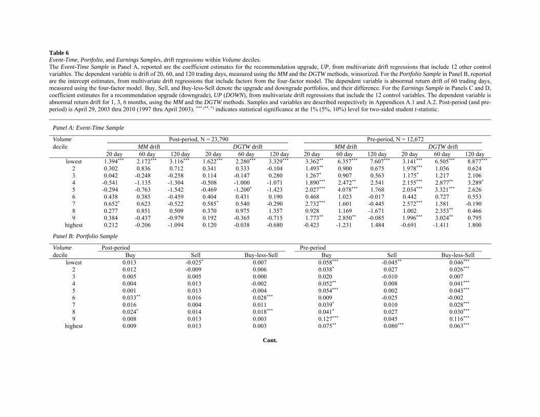
Table 6 Event-Time, Portfolio, and Earnings Samples, drift regressions within Volume deciles. The Event-Time Sample in Panel A, reported are the coefficient estimates for the recommendation upgrade, UP, from multivariate drift regressions that include 12 other control variables. The dependent variable is drift of 20, 60, and 120 trading days, measured using the MM and the DGTW methods, winsorized. For the Portfolio Sample in Panel B, reported are the intercept estimates, from multivariate drift regressions that include factors from the four-factor model. The dependent variable is abnormal return drift of 60 trading days, measured using the four-factor model. Buy, Sell, and Buy-less-Sell denote the upgrade and downgrade portfolios, and their difference. For the Earnings Sample in Panels C and D, coefficient estimates for a recommendation upgrade (downgrade), UP (DOWN), from multivariate drift regressions that include the 12 control variables. The dependent variable is abnormal return drift for 1, 3, 6 months, using the MM and the DGTW methods. Samples and variables are described respectively in Appendices A.1 and A.2. Post-period (and pre-period) is April 29, 2003 thru 2010 (1997 thru April 2003). *** (**, *) indicates statistical significance at the 1% (5%, 10%) level for two-sided student t-statistic.
Panel A: Event-Time Sample
Volume Post-period, N = 23,790 Pre-period, N = 12,672 decile MM drift DGTW drift MM drift DGTW drift 20 day 60 day 120 day 20 day 60 day 120 day 20 day 60 day 120 day 20 day 60 day 120 day
lowest 1.394*** 2.172*** 3.116*** 1.622*** 2.280*** 3.329*** 3.362** 6.357*** 7.607*** 3.141*** 6.505*** 8.877*** 2 0.302 0.836 0.712 0.341 0.333 -0.104 1.493** 0.900 0.675 1.978*** 1.036 0.624 3 0.042 -0.248 -0.258 0.114 -0.147 0.280 1.267* 0.907 0.563 1.175* 1.217 2.106 4 -0.541 -1.135 -1.304 -0.508 -1.000 -1.071 1.890*** 2.472** 2.541 2.155*** 2.877** 3.289* 5 -0.294 -0.763 -1.542 -0.469 -1.200* -1.423 2.027*** 4.078*** 1.768 2.034*** 3.321*** 2.626 6 0.438 0.385 -0.459 0.404 0.431 0.190 0.468 1.023 -0.017 0.442 0.727 0.553 7 0.652* 0.623 -0.522 0.585* 0.540 -0.290 2.732*** 1.601 -0.445 2.572*** 1.581 -0.190 8 0.277 0.851 0.509 0.370 0.975 1.357 0.928 1.169 -1.671 1.002 2.353** 0.466 9 0.384 -0.437 -0.979 0.192 -0.365 -0.715 1.773** 2.850** -0.085 1.996*** 3.024** 0.795
highest 0.212 -0.206 -1.094 0.120 -0.038 -0.680 -0.423 -1.231 1.484 -0.691 -1.411 1.800
Panel B: Portfolio Sample
Volume Post-period Pre-period decile Buy Sell Buy-less-Sell Buy Sell Buy-less-Sell
lowest 0.013 -0.025* 0.007 0.058*** -0.045** 0.046*** 2 0.012 -0.009 0.006 0.038* 0.027 0.026*** 3 0.005 0.005 0.000 0.020 -0.010 0.007 4 0.004 0.013 -0.002 0.052** 0.008 0.041*** 5 0.001 0.013 -0.004 0.054*** 0.002 0.043*** 6 0.033** 0.016 0.028*** 0.009 -0.025 -0.002 7 0.016 0.004 0.011 0.039* 0.010 0.028*** 8 0.024* 0.014 0.018*** 0.041* 0.027 0.030*** 9 0.008 0.013 0.003 0.127*** 0.045 0.116***
highest 0.009 0.013 0.003 0.075** 0.080*** 0.063***
Cont.
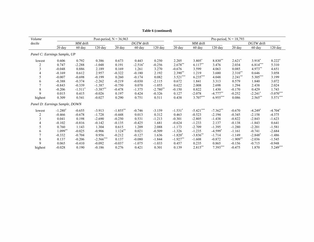
Table 6 (continued)
Volume Post-period, N = 36,963 Pre-period, N = 18,793 decile MM drift DGTW drift MM drift DGTW drift 20 day 60 day 120 day 20 day 60 day 120 day 20 day 60 day 120 day 20 day 60 day 120 day
Panel C: Earnings Sample, UP
lowest 0.606 0.792 0.386 0.673 0.443 0.250 2.205 3.805* 8.830** 2.621* 3.918* 8.222* 2 0.747 -2.288 -1.048 0.191 -2.516* -0.256 2.678** 6.117** 3.476 2.034 6.814*** 5.310 3 -0.048 0.886 2.189 0.169 1.261 3.270 -0.676 3.599 4.063 0.085 4.973** 4.651 4 -0.169 0.612 2.957 -0.322 -0.180 2.192 2.390** 1.219 3.680 2.310** 0.646 3.058 5 -0.007 -0.698 -0.199 0.260 -0.174 0.082 3.521*** 6.235*** 4.048 2.241** 5.305*** 3.199 6 -0.388 -0.374 -2.262 -0.219 -0.030 -2.115 0.672 1.841 3.313 0.579 1.840 3.072 7 -0.843 -0.339 -1.387 -0.750 0.070 -1.055 0.622 2.008 2.698 1.294 2.438 2.024 8 -0.206 -1.511* -3.387** -0.478 -1.375 -2.780** -0.150 0.822 1.430 -0.170 0.429 1.743 9 0.015 0.415 -0.026 0.197 0.424 -0.326 0.127 -2.078 -4.777** -0.252 -2.241* -5.070***
highest 0.309 0.541 -0.027 0.290 0.751 0.511 0.438 3.707*** 6.955*** 0.086 2.565** 5.571***
Panel D: Earnings Sample, DOWN
lowest -1.280* -0.655 -3.913 -1.855** -0.746 -3.159 -1.531* -5.421*** -7.362** -0.670 -4.249* -4.704* 2 -0.466 -0.678 -1.728 -0.448 0.013 0.312 0.463 -0.523 -2.194 -0.345 -2.158 -4.375 3 0.041 0.198 -2.690 -0.250 0.531 -1.213 -0.301 -2.805 -1.438 -0.822 -2.843 -1.623 4 -0.102 -0.816 -0.142 -0.135 -0.425 1.681 -0.624 -1.233 2.137 -0.138 -1.843 0.641 5 0.760 1.143 1.304 0.615 1.209 2.088 -1.173 -2.709 -1.395 -1.280 -2.201 -1.581 6 1.099** -0.025 -0.906 1.124** 0.021 -0.509 -1.326 -1.235 -4.599* -1.161 -0.741 -2.684 7 -0.332 -0.704 0.956 -0.212 -0.127 1.636 -1.820* -3.836** -1.714 -1.149 -2.848* -1.486 8 0.137 -0.206 -2.566*** 0.137 -0.080 -1.844 -1.927** -1.608 -0.872 -1.909** -2.036 -1.545 9 0.065 -0.410 -0.092 -0.037 -1.075 -1.033 0.457 0.235 0.865 -0.156 -0.715 -0.948
highest -0.028 0.190 -0.186 0.276 0.421 0.301 0.139 2.815** 7.393*** -0.475 1.870 5.249***

Table 7 Event-Time, Portfolio, and Earnings Samples, drift regressions within Firm Size deciles. The Event-Time Sample in Panel A, reported are the coefficient estimates for the recommendation upgrade, UP, from multivariate drift regressions that include 12 other control variables. The dependent variable is drift of 20, 60, and 120 trading days, measured using the MM and the DGTW methods, winsorized. For the Portfolio Sample in Panel B, reported are the intercept estimates, from multivariate drift regressions that include factors from the four-factor model. The dependent variable is abnormal return drift of 60 trading days, measured using the four-factor model. Buy, Sell, and Buy-less-Sell denote the upgrade and downgrade portfolios, and their difference. For the Earnings Sample in Panels C and D, coefficient estimates for a recommendation upgrade (downgrade), UP (DOWN), from multivariate drift regressions that include the 12 control variables. The dependent variable is abnormal return drift for 1, 3, 6 months, using the MM and the DGTW methods. Samples and variables are described respectively in Appendices A.1 and A.2. Post-period (and pre-period) is April 29, 2003 thru 2010 (1997 thru April 2003). *** (**, *) indicates statistical significance at the 1% (5%, 10%) level for two-sided student t-statistic.
Panel A: Event-Time Sample
Firm Size Post-period, N = 23,790 Pre-period, N = 12,672 decile MM drift DGTW drift MM drift DGTW drift 20 day 60 day 120 day 20 day 60 day 120 day 20 day 60 day 120 day 20 day 60 day 120 day
lowest 1.838*** 2.346*** 2.572* 1.903*** 2.474*** 3.013*** 2.898*** 5.102*** 6.513*** 2.636*** 5.321*** 7.366*** 2 0.404 0.115 0.195 0.198 -0.425 -0.483 2.126*** 3.235** 3.816* 2.345*** 3.141** 4.775** 3 0.441 0.386 -0.897 0.251 0.128 -0.617 1.189 2.552* 0.880 0.940 2.169 1.136 4 -0.350 -0.127 -0.438 -0.207 -0.315 -0.317 1.057*** 1.815 0.403 1.212* 1.224 0.774 5 -0.159 -0.153 -0.748 -0.155 -0.123 -0.503 2.083*** 1.563 1.615 2.049*** 3.019*** 4.263*** 6 -0.237 -0.738 -1.430 -0.194 -0.766 -0.890 1.914 1.455 0.035 2.098*** 1.485 0.606 7 -0.364 -0.943 -1.800** -0.357 -0.777 -1.081 1.132*** 1.416 -0.249 1.027 1.381 0.259 8 0.674** 1.133** 0.633 0.700**\ 1.073** 0.854 1.987*** 2.451** 1.741 2.304*** 3.143*** 2.958* 9 0.629** 0.410 0.784 0.714*** 0.811 1.559** 1.549 0.436 -0.728 1.417** 0.009 -0.825
highest -0.055 -0.423 -0.380 -0.163 -0.431 -0.575 -0.327 0.789 -0.023 -0.269 0.920 1.194
Panel B: Portfolio Sample
Firm Size Post-period Pre-period decile Buy Sell Buy-less-Sell Buy Sell Buy-less-Sell
lowest 0.032* -0.013 0.026*** 0.064*** -0.023 0.051*** 2 0.011 0.008 0.006 0.068*** 0.021 0.053*** 3 -0.002 -0.002 -0.007 0.066*** 0.014 0.052*** 4 -0.006 0.000 -0.012** 0.043* 0.024 0.030*** 5 0.002 0.002 -0.003 0.060*** 0.016 0.047*** 6 0.017 0.023* 0.011** 0.034 0.005 0.022** 7 -0.001 0.009 -0.006 0.042* 0.015 0.031*** 8 0.029*** 0.009 0.024*** 0.076*** 0.025 0.064*** 9 0.017* 0.010 0.012** 0.031 -0.001 0.019**
highest 0.001 0.007 -0.004 0.023 0.038* 0.011
Cont.

Table 7 (continued)
Firm Size Post-period, N = Pre-period, N = decile MM drift DGTW drift MM drift DGTW drift 20 day 60 day 120 day 20 day 60 day 120 day 20 day 60 day 120 day 20 day 60 day 120 day
Panel C: Earnings Sample, UP
lowest 0.307 2.953 4.135 0.757 2.854 4.532 -0.632 3.380 -0.354 0.373 5.578 -1.499 2 0.146 -1.533 0.633 0.044 -1.455 0.487 2.698 4.775 6.478 2.714* 6.216** 6.657 3 0.831 -1.618 -2.934 0.558 -1.499 -2.390 -0.350 0.840 -0.346 -0.060 1.707 1.057 4 0.561 0.930 1.595 0.307 0.186 1.243 1.878 4.322 7.183** 1.280 3.650* 6.323** 5 0.830 -0.327 -1.259 0.872 -0.051 -0.931 3.194*** 5.503*** 11.721*** 2.339** 4.583*** 9.713 6 -0.870 -1.967** -4.487*** -0.390 -1.438 -3.964*** 1.912** 2.305 2.634 2.156** 2.069 2.219 7 -0.904** -0.950 -2.299* -0.659 0.014 -1.060 -0.287 0.282 -1.161 -0.255 0.439 -0.591 8 -0.348 0.377 -0.120 -0.512 0.089 -0.467 1.155 1.588 2.524 0.753 0.527 2.362 9 -0.085 0.489 0.119 -0.232 0.536 0.245 0.362 2.036 2.293 0.307 1.787 1.709
highest 0.091 0.595 0.767 0.045 0.649 1.110 0.180 0.935 1.277 -0.007 0.396 0.193
Panel D: Earnings Sample, DOWN
lowest -2.336** -2.476 -4.583 -2.567* -2.652 -2.848 -2.089 -6.878** -9.234* -2.910* -6.793** -6.961 2 -0.756 -1.979 -3.993 -0.228 -0.004 -0.623 0.961 -5.863* -3.834 1.243 -5.828** -2.389 3 -1.090 1.708 2.743 -1.158* 1.929 3.7 -3.012** -3.134 -4.155 -2.852** -2.134 -1.816 4 0.343 0.630 -0.204 0.224 0.540 1.173 -2.680** -0.147 5.324* -2.260** 0.265 3.493 5 1.128** -0.786 -0.940 0.641 -0.617 -0.161 0.362 -3.072* -1.939 0.563 -2.420 -1.890 6 0.921* 0.671 0.524 1.006** 0.624 0.759 -0.585 -0.142 0.468 -0.410 0.259 1.269 7 0.462 -1.001 -2.162 0.335 -0.676 -1.328 -1.001 -2.243 -4.969** -1.046 -2.786* -5.019** 8 0.505 0.791 -0.852 0.589 0.671 -0.959 -0.170 0.204 3.539* -0.480 -0.208 2.365 9 0.023 -1.013 -1.789 0.098 -1.361* -2.412** 0.557 0.783 3.898** 0.011 -0.276 0.475
highest -0.331 0.110 0.888 -0.178 0.153 1.302 -0.020 1.297 2.234 -0.529 0.757 1.263

Table 8 Event-Time, Portfolio, and Earnings Samples, drift regressions within Analyst Coverage deciles. The Event-Time Sample in Panel A, reported are the coefficient estimates for the recommendation upgrade, UP, from multivariate drift regressions that include 12 other control variables. The dependent variable is drift of 20, 60, and 120 trading days, measured using the MM and the DGTW methods, winsorized. For the Portfolio Sample in Panel B, reported are the intercept estimates, from multivariate drift regressions that include factors from the four-factor model. The dependent variable is abnormal return drift of 20, 60, and 120 trading days, using the MM and the DGTW methods, winsorized. Buy, Sell, and Buy-less-Sell denote the upgrade and downgrade portfolios, and their difference. For the Earnings Sample in Panels C and D, coefficient estimates for a recommendation upgrade (downgrade), UP (DOWN), from multivariate drift regressions that include the 12 control variables. The dependent variable is abnormal return drift for 1, 3, 6 months, using the MM and the DGTW methods. Samples and variables are described respectively in Appendices A.1 and A.2. Post-period (and pre-period) is April 29, 2003 thru 2010 (1997 thru April 2003). *** (**, *) indicates statistical significance at the 1% (5%, 10%) level for two-sided student t-statistic.
Panel A: Event-Time Sample
Coverage Post-period, N = 23,790 Pre-period, N = 12,672 decile MM drift DGTW drift MM drift DGTW drift 20 day 60 day 120 day 20 day 60 day 120 day 20 day 60 day 120 day 20 day 60 day 120 day
lowest 1.814*** 1.983*** 2.161* 1.968*** 2.065*** 2.455** 2.984*** 3.912*** 5.086** 3.137*** 4.350*** 6.882*** 2 0.099 -0.205 0.007 0.233 -0.225 0.184 2.624*** 4.877*** 6.487*** 2.564*** 4.428*** 4.915*** 3 0.186 -0.099 -0.478 0.195 -0.217 -0.363 1.744** 2.846** 1.747 1.898*** 2.907*** 2.238 4 -0.094 0.335 -0.480 0.116 0.354 -0.143 1.464* 0.764 -1.649 1.546** 0.966 0.155 5 -0.081 0.705 -0.245 -0.072 0.499 -0.582 1.641** 3.197*** 1.290 1.479** 2.932*** 1.902 6 0.034 -0.640 -2.095** -0.026 -0.715 -1.505 0.599 2.414** 0.922 0.830 2.673** 2.203 7 0.472 0.285 0.233 0.228 0.026 0.440 0.846 -1.059 -0.594 0.874 -0.117 1.444 8 0.361 0.547 0.707 0.281 0.659 1.299 0.719 0.045 -3.804** 0.853 0.139 -2.757* 9 0.319 -0.251 -0.628 -0.009 -0.349 -0.108 1.006 0.395 -1.464 0.921 0.588 -0.267
highest -0.382 -0.634 -1.167 -0.257 -0.388 -0.986 1.673** 2.848** 4.999*** 1.440 2.587** 4.359**
Panel B: Portfolio Sample
Coverage Post-period Pre-period decile Buy Sell Buy-less-Sell Buy Sell Buy-less-Sell
lowest 0.026** -0.007 0.021*** 0.050** 0.010 0.036*** 2 -0.001 0.001 -0.006 0.046** -0.031 0.031*** 3 0.009 0.003 0.003 0.035 -0.024 0.022** 4 0.003 -0.005 -0.002 0.034 0.028 0.020** 5 0.005 -0.004 -0.001 0.060*** -0.014 0.047*** 6 0.006 0.012 0.001 0.053** -0.009 0.040*** 7 0.016 0.021* 0.010** 0.019 0.031 0.003 8 0.031** 0.013 0.026*** 0.032 0.032 0.019* 9 0.014 0.017 0.002 0.072** 0.064*** 0.059***
highest -0.006 0.003 -0.011** 0.094*** 0.050* 0.081***
Cont.
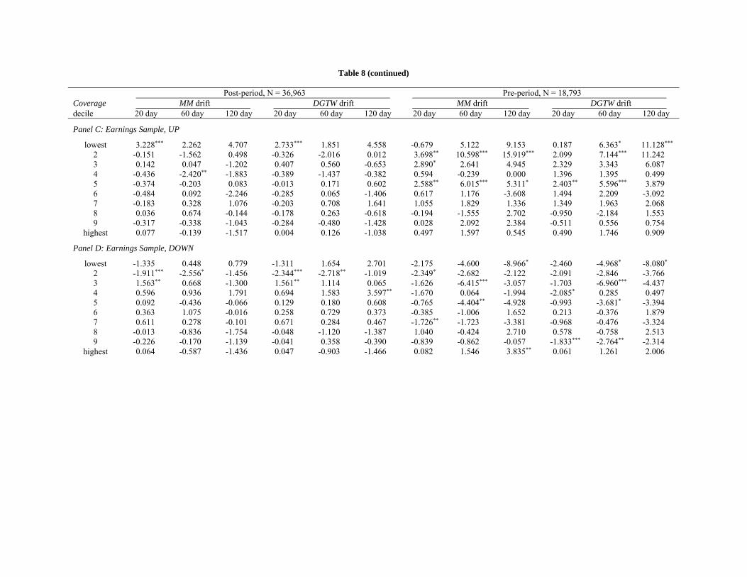
Table 8 (continued)
Post-period, N = 36,963 Pre-period, N = 18,793 Coverage MM drift DGTW drift MM drift DGTW drift decile 20 day 60 day 120 day 20 day 60 day 120 day 20 day 60 day 120 day 20 day 60 day 120 day
Panel C: Earnings Sample, UP
lowest 3.228*** 2.262 4.707 2.733*** 1.851 4.558 -0.679 5.122 9.153 0.187 6.363* 11.128*** 2 -0.151 -1.562 0.498 -0.326 -2.016 0.012 3.698** 10.598*** 15.919*** 2.099 7.144*** 11.242 3 0.142 0.047 -1.202 0.407 0.560 -0.653 2.890* 2.641 4.945 2.329 3.343 6.087 4 -0.436 -2.420** -1.883 -0.389 -1.437 -0.382 0.594 -0.239 0.000 1.396 1.395 0.499 5 -0.374 -0.203 0.083 -0.013 0.171 0.602 2.588** 6.015*** 5.311* 2.403** 5.596*** 3.879 6 -0.484 0.092 -2.246 -0.285 0.065 -1.406 0.617 1.176 -3.608 1.494 2.209 -3.092 7 -0.183 0.328 1.076 -0.203 0.708 1.641 1.055 1.829 1.336 1.349 1.963 2.068 8 0.036 0.674 -0.144 -0.178 0.263 -0.618 -0.194 -1.555 2.702 -0.950 -2.184 1.553 9 -0.317 -0.338 -1.043 -0.284 -0.480 -1.428 0.028 2.092 2.384 -0.511 0.556 0.754
highest 0.077 -0.139 -1.517 0.004 0.126 -1.038 0.497 1.597 0.545 0.490 1.746 0.909
Panel D: Earnings Sample, DOWN
lowest -1.335 0.448 0.779 -1.311 1.654 2.701 -2.175 -4.600 -8.966* -2.460 -4.968* -8.080* 2 -1.911*** -2.556* -1.456 -2.344*** -2.718** -1.019 -2.349* -2.682 -2.122 -2.091 -2.846 -3.766 3 1.563** 0.668 -1.300 1.561** 1.114 0.065 -1.626 -6.415*** -3.057 -1.703 -6.960*** -4.437 4 0.596 0.936 1.791 0.694 1.583 3.597** -1.670 0.064 -1.994 -2.085* 0.285 0.497 5 0.092 -0.436 -0.066 0.129 0.180 0.608 -0.765 -4.404** -4.928 -0.993 -3.681* -3.394 6 0.363 1.075 -0.016 0.258 0.729 0.373 -0.385 -1.006 1.652 0.213 -0.376 1.879 7 0.611 0.278 -0.101 0.671 0.284 0.467 -1.726** -1.723 -3.381 -0.968 -0.476 -3.324 8 -0.013 -0.836 -1.754 -0.048 -1.120 -1.387 1.040 -0.424 2.710 0.578 -0.758 2.513 9 -0.226 -0.170 -1.139 -0.041 0.358 -0.390 -0.839 -0.862 -0.057 -1.833*** -2.764** -2.314
highest 0.064 -0.587 -1.436 0.047 -0.903 -1.466 0.082 1.546 3.835** 0.061 1.261 2.006
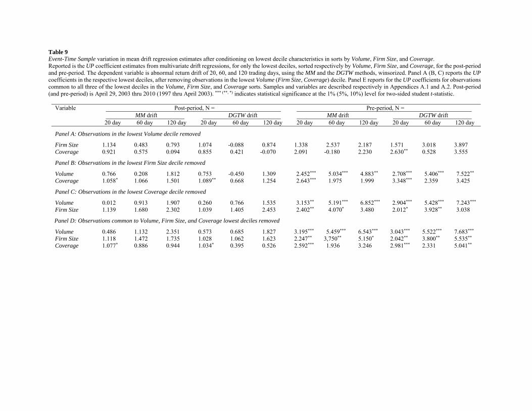
Table 9 Event-Time Sample variation in mean drift regression estimates after conditioning on lowest decile characteristics in sorts by Volume, Firm Size, and Coverage. Reported is the UP coefficient estimates from multivariate drift regressions, for only the lowest deciles, sorted respectively by Volume, Firm Size, and Coverage, for the post-period and pre-period. The dependent variable is abnormal return drift of 20, 60, and 120 trading days, using the MM and the DGTW methods, winsorized. Panel A (B, C) reports the UP coefficients in the respective lowest deciles, after removing observations in the lowest Volume (Firm Size, Coverage) decile. Panel E reports for the UP coefficients for observations common to all three of the lowest deciles in the Volume, Firm Size, and Coverage sorts. Samples and variables are described respectively in Appendices A.1 and A.2. Post-period (and pre-period) is April 29, 2003 thru 2010 (1997 thru April 2003). *** (**, *) indicates statistical significance at the 1% (5%, 10%) level for two-sided student t-statistic.
Variable Post-period, N = Pre-period, N = MM drift DGTW drift MM drift DGTW drift 20 day 60 day 120 day 20 day 60 day 120 day 20 day 60 day 120 day 20 day 60 day 120 day
Panel A: Observations in the lowest Volume decile removed
Firm Size 1.134 0.483 0.793 1.074 -0.088 0.874 1.338 2.537 2.187 1.571 3.018 3.897 Coverage 0.921 0.575 0.094 0.855 0.421 -0.070 2.091 -0.180 2.230 2.630** 0.528 3.555
Panel B: Observations in the lowest Firm Size decile removed
Volume 0.766 0.208 1.812 0.753 -0.450 1.309 2.452*** 5.034*** 4.883** 2.708*** 5.406*** 7.522** Coverage 1.058* 1.066 1.501 1.089** 0.668 1.254 2.643*** 1.975 1.999 3.348*** 2.359 3.425
Panel C: Observations in the lowest Coverage decile removed
Volume 0.012 0.913 1.907 0.260 0.766 1.535 3.153** 5.191*** 6.852*** 2.904*** 5.428*** 7.243*** Firm Size 1.139 1.680 2.302 1.039 1.405 2.453 2.402** 4.070* 3.480 2.012* 3.928** 3.038
Panel D: Observations common to Volume, Firm Size, and Coverage lowest deciles removed
Volume 0.486 1.132 2.351 0.573 0.685 1.827 3.195*** 5.459*** 6.543*** 3.043*** 5.522*** 7.683*** Firm Size 1.118 1.472 1.735 1.028 1.062 1.623 2.247** 3,750** 5.150* 2.042** 3.800** 5.535** Coverage 1.077* 0.886 0.944 1.034* 0.395 0.526 2.592*** 1.936 3.246 2.981*** 2.331 5.041**
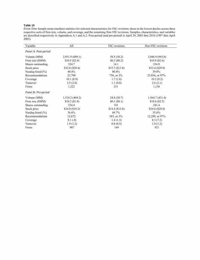
Table 10 Event-Time Sample mean (median) statistics for selected characteristics for VSC revisions; those in the lowest deciles across three respective sorts of firm size, volume, and coverage, and the remaining Non-VSC revisions. Samples, characteristics, and variables are described respectively in Appendices A.1 and A.2. Post-period (and pre-period) is April 29, 2003 thru 2010 (1997 thru April 2003).
Variable All VSC revisions Non-VSC revisions
Panel A: Post-period
Volume (MM) 2,951.9 (889.1) 58.5 (38.2) 3,046.9 (943.0) Firm size ($MM) $10.5 ($2.4) $0.2 ($0.2) $10.8 ($2.6) Shares outstanding 324.7 14.1 334.9 Stock price $32.8 ($28.4) $15.7 ($13.8) $33.4 ($29.0) Nasdaq-listed (%) 40.4% 80.4% 39.0% Recommendations 23,790 756, or 3% 23,034, or 97% Coverage 10.1 (8.9) 1.7 (1.6) 10.3 (9.2) Turnover 2.5 (2.0) 1.1 (0.8) 2.6 (2.1) Firms 1,222 231 1,138
Panel B: Pre-period
Volume (MM) 1,518.2 (404.2) 24.8 (20.7) 1,564.7 (431.4) Firm size ($MM) $10.3 ($1.8) $0.1 ($0.1) $10.6 ($2.5) Shares outstanding 234.4 9.8 241.4 Stock price $34.0 ($19.3) $14.4 ($13.8) $34.6 ($29.8) Nasdaq-listed (%) 36.6% 69.7% 35.6% Recommendations 12,672 383, or 3% 12,289, or 97% Coverage 8.1 (.0) 1.4 (1.3) 8.3 (7.2) Turnover 1.9 (1.2) 0.8 (0.5) 1.9 (1.2) Firms 987 169 921

Table 11 Event-Time, Portfolio, and Earnings Samples, drift regressions within Turnover deciles. Reported are the coefficient estimates for the recommendation upgrade, UP, from multivariate drift regressions that include 12 other control variables. The dependent variable is drift of 20, 60, and 120 trading days, measured using the MM and the DGTW methods, winsorized. Panel A reports the UP coefficients in the post-period and pre-periods, and Panel B reports the UP coefficients in the post-period after removing all VSC revisions. For the Portfolio Sample in Panel C, reported are the intercept estimates, from multivariate drift regressions that include factors from the four-factor model. The dependent variable is abnormal return drift of 60 trading days, measured using the four-factor model. Buy, Sell, and Buy-less-Sell denote the upgrade and downgrade portfolios, and their difference. For the Earnings Sample in Panels D and E, coefficient estimates for a recommendation upgrade (downgrade), UP (DOWN), from multivariate drift regressions that include the 12 control variables. The dependent variable is abnormal return drift for 1, 3, 6 months, using the MM and the DGTW methods. Samples and variables are described respectively in Appendices A.1 and A.2. Post-period (and pre-period) is April 29, 2003 thru 2010 (1997 thru April 2003). *** (**, *) indicates statistical significance at the 1% (5%, 10%) level for two-sided student t-statistic.
Turnover Post-period, N = 23,790 Pre-period, N = 12,672 decile MM drift DGTW drift MM drift DGTW drift 20 day 60 day 120 day 20 day 60 day 120 day 20 day 60 day 120 day 20 day 60 day 120 day
Panel A: Event-Time Sample UP coefficient estimates, by turnover decile
lowest 1.038*** 2.125*** 2.961*** 0.931*** 1.737*** 2.442*** 2.633*** 4.134*** 5.333*** 3.081*** 4.821*** 7.156*** 2 0.512* 0.639 0.282 0.599* 0.736 0.386 2.535*** 1.768 -0.227 2.699*** 2.188* 1.304 3 -0.071 0.007 1.454 -0.028 -0.005 1.374 1.131* 1.913* 1.366 1.810*** 2.335** 2.634* 4 0.309 -0.048 -0.459 0.448 -0.189 -0.666 1.327* 2.717** 3.121* 1.803*** 3.474*** 3.939** 5 0.142 0.191 -0.384 0.125 0.121 -0.517 2.216*** 0.551 -1.312 2.052*** 0.831 0.094 6 -0.425 -0.517 -1.532 -0.193 -0.231 -0.651 1.464** -0.142 -1.359 1.756** 0.189 -0.372 7 0.357 0.383 -0.520 0.251 0.032 -0.323 2.111** 1.108 2.236 2.055*** 1.234 2.831 8 0.053 -1.255 -1.275 -0.135 -1.235 -1.223 2.464*** 3.742** 2.175 2.027** 3.468** 2.315 9 0.465 1.526* 1.325 0.470 1.598* 2.269* 0.483 3.902** -0.994 0.141 2.513 -0.508
highest -0.088 -1.525 -3.431** -0.172 -1.394 -2.292* 0.475 1.986 1.084 0.386 1.379 0.626
Cont.
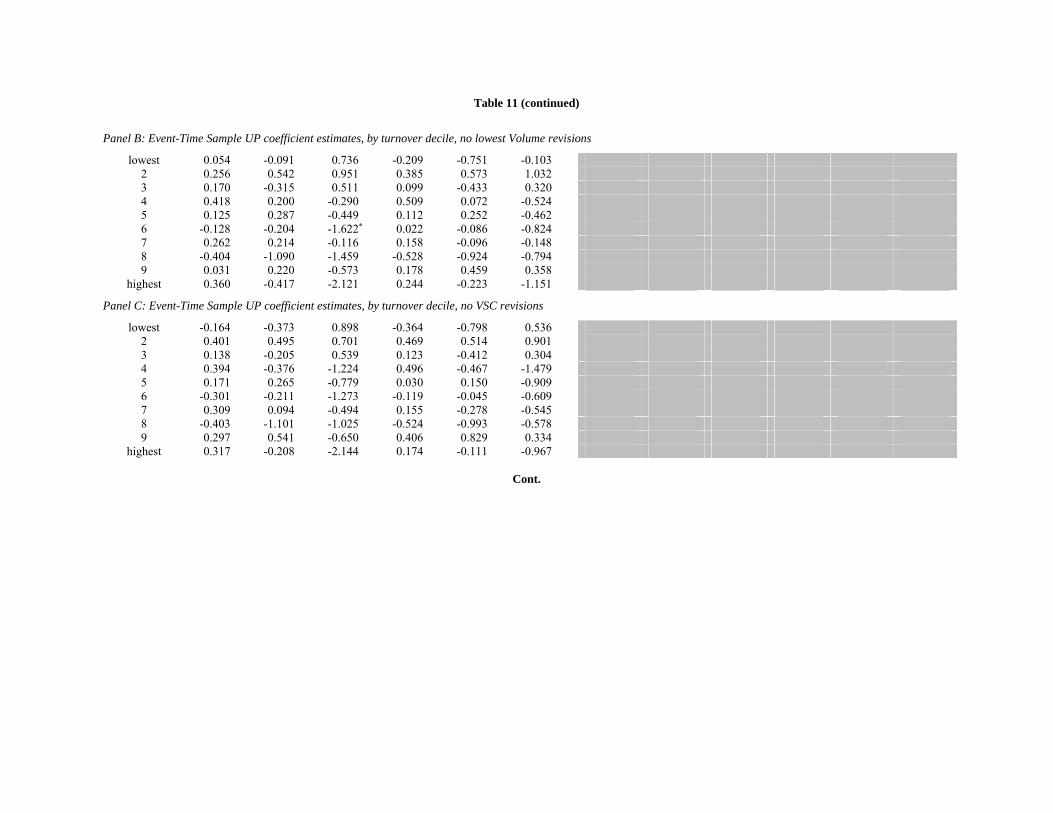
Table 11 (continued)
Panel B: Event-Time Sample UP coefficient estimates, by turnover decile, no lowest Volume revisions
lowest 0.054 -0.091 0.736 -0.209 -0.751 -0.103 2 0.256 0.542 0.951 0.385 0.573 1.032 3 0.170 -0.315 0.511 0.099 -0.433 0.320 4 0.418 0.200 -0.290 0.509 0.072 -0.524 5 0.125 0.287 -0.449 0.112 0.252 -0.462 6 -0.128 -0.204 -1.622* 0.022 -0.086 -0.824 7 0.262 0.214 -0.116 0.158 -0.096 -0.148 8 -0.404 -1.090 -1.459 -0.528 -0.924 -0.794 9 0.031 0.220 -0.573 0.178 0.459 0.358
highest 0.360 -0.417 -2.121 0.244 -0.223 -1.151
Panel C: Event-Time Sample UP coefficient estimates, by turnover decile, no VSC revisions
lowest -0.164 -0.373 0.898 -0.364 -0.798 0.536 2 0.401 0.495 0.701 0.469 0.514 0.901 3 0.138 -0.205 0.539 0.123 -0.412 0.304 4 0.394 -0.376 -1.224 0.496 -0.467 -1.479 5 0.171 0.265 -0.779 0.030 0.150 -0.909 6 -0.301 -0.211 -1.273 -0.119 -0.045 -0.609 7 0.309 0.094 -0.494 0.155 -0.278 -0.545 8 -0.403 -1.101 -1.025 -0.524 -0.993 -0.578 9 0.297 0.541 -0.650 0.406 0.829 0.334
highest 0.317 -0.208 -2.144 0.174 -0.111 -0.967
Cont.

Table 11 (continued)
Panel C: Portfolio Sample
Turnover Post-period Pre-period decile Buy Sell Buy-less-Sell Buy Sell Buy-less-Sell
lowest 0.023** -0.010 0.011* 0.047*** -0.028 0.031*** 2 0.007 -0.016* 0.004 0.032* -0.034** 0.013 3 0.018 0.012 0.001 0.007 -0.026* -0.010 4 0.013 0.013 0.009 0.035** -0.004 0.018* 5 0.020** 0.004 0.015*** 0.009 0.008 -0.008 6 0.001 0.009 -0.003 0.021 0.030 0.004 7 0.003 -0.004 -0.001 0.008 0.014 -0.011 8 0.008 0.023** 0.004 0.064** 0.036 0.046*** 9 0.023 0.020 0.002 0.116*** 0.050 0.098***
highest -0.007 -0.004 -0.011 0.159*** 0.137*** 0.141*** Turnover Post-period Pre-period decile MM drift DGTW drift MM drift DGTW drift 20 day 60 day 120 day 20 day 60 day 120 day 20 day 60 day 120 day 20 day 60 day 120 day
Panel D: Earnings Sample, UP
lowest -0.143 -0.901 -2.569 0.315 0.236 -0.923 0.606 -0.208 4.609 2.053 3.488 11.248 2 0.509 0.059 -0.724 0.389 0.445 0.614 2.050 4.481* -1.160 2.662 4.973 0.620 3 -0.764 -0.441 -1.571 -0.656 -0.380 -1.354 -0.079 0.383 0.271 -0.292 1.048 1.425 4 -0.296 1.500 0.496 -0.165 1.784 1.394 0.211 2.741 2.461 0.235 2.285 2.156 5 0.273 0.375 0.080 0.297 0.430 -0.068 0.117 -0.880 -0.547 0.851 0.507 1.225 6 -0.226 0.984 1.719 -0.303 1.297 2.041 0.612 3.306* 2.636 0.278 3.130 1.383 7 -0.181 -1.151 -1.642 -0.103 -0.908 -0.902 0.837 1.134 0.049 0.864 1.685 0.126 8 -0.396 -0.484 -0.834 -0.344 -0.228 -0.673 0.986 -1.362 -2.667 0.514 -2.003 -3.321 9 -0.109 -1.534 -3.213 -0.085 -1.504 -2.746 2.410** 4.608** 5.695* 2.603 4.223 5.475
highest 0.033 -0.987 -1.989 -0.016 -0.850 -1.977 0.145 2.060 7.137* -0.091 1.241 5.744
Panel E: Earnings Sample, DOWN
lowest -0.863 -3.031 -5.530* -0.404 -1.727 -3.618 -1.464 -4.572* -7.830* -0.595 -2.871 -5.850 2 -0.361 -1.721 -0.975 -0.394 -0.991 1.241 -1.143 -2.706 -4.715 -2.154** -3.099 -5.290 3 -0.752 -0.893 -2.778 -0.549 -0.368 -1.611 -0.497 -1.608 -0.594 -0.551 -1.379 -1.321 4 -0.393 -0.361 -1.649 0.017 0.274 0.017 -1.681 -3.288 1.219 -1.718 -3.466* 0.442 5 -0.098 -1.394 -3.013* -0.159 -0.532 -1.060 -0.687 -1.559 -3.588 -0.691 -1.253 -3.037 6 0.514 0.458 1.023 0.329 0.392 1.625 -0.167 -0.811 3.118 -0.374 -0.725 2.001 7 0.283 -0.007 1.508 0.367 0.174 1.821 -0.143 -0.656 -2.592 -0.365 -0.425 -2.801 8 1.205** 1.624 1.614 1.029** 1.507 2.096 0.257 -1.482 2.150 -0.551 -2.656 -0.374 9 0.519 0.862 1.220 0.384 0.869 1.763 0.131 0.344 2.218 0.218 -0.346 1.810
highest -0.545 -1.345 -3.797** -0.418 -1.630 -3.961** -1.938 -1.716 1.410 -1.905 -1.604 0.814
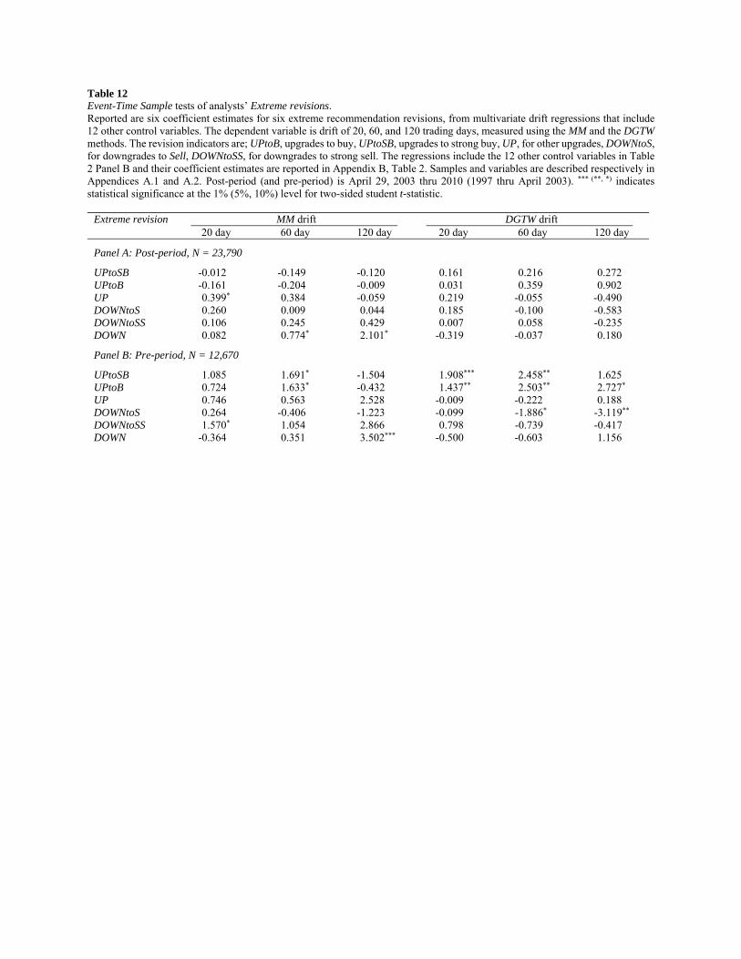
Table 12 Event-Time Sample tests of analysts’ Extreme revisions. Reported are six coefficient estimates for six extreme recommendation revisions, from multivariate drift regressions that include 12 other control variables. The dependent variable is drift of 20, 60, and 120 trading days, measured using the MM and the DGTW methods. The revision indicators are; UPtoB, upgrades to buy, UPtoSB, upgrades to strong buy, UP, for other upgrades, DOWNtoS, for downgrades to Sell, DOWNtoSS, for downgrades to strong sell. The regressions include the 12 other control variables in Table 2 Panel B and their coefficient estimates are reported in Appendix B, Table 2. Samples and variables are described respectively in Appendices A.1 and A.2. Post-period (and pre-period) is April 29, 2003 thru 2010 (1997 thru April 2003). *** (**, *) indicates statistical significance at the 1% (5%, 10%) level for two-sided student t-statistic.
Extreme revision MM drift DGTW drift 20 day 60 day 120 day 20 day 60 day 120 day
Panel A: Post-period, N = 23,790
UPtoSB -0.012 -0.149 -0.120 0.161 0.216 0.272 UPtoB -0.161 -0.204 -0.009 0.031 0.359 0.902 UP 0.399* 0.384 -0.059 0.219 -0.055 -0.490 DOWNtoS 0.260 0.009 0.044 0.185 -0.100 -0.583 DOWNtoSS 0.106 0.245 0.429 0.007 0.058 -0.235 DOWN 0.082 0.774* 2.101* -0.319 -0.037 0.180
Panel B: Pre-period, N = 12,670
UPtoSB 1.085 1.691* -1.504 1.908*** 2.458** 1.625 UPtoB 0.724 1.633* -0.432 1.437** 2.503** 2.727* UP 0.746 0.563 2.528 -0.009 -0.222 0.188 DOWNtoS 0.264 -0.406 -1.223 -0.099 -1.886* -3.119** DOWNtoSS 1.570* 1.054 2.866 0.798 -0.739 -0.417 DOWN -0.364 0.351 3.502*** -0.500 -0.603 1.156

Table 13 Event-Time Sample and Portfolio Sample drift regressions within brokerage firm Reputation deciles. Reported in Panel A (B) are UP coefficient estimates for the Event-Time Sample (Buy and Sell coefficient estimates for the Portfolio Sample), for the post-period and pre-period, from multivariate drift regressions estimated for all observations and within each decile sorted on brokerage firm Reputation. The dependent variable is abnormal return drift of 20, 60, and 120 trading days (60 trading days) using MM and DGTW (Portfolio) methods, winsorized. Samples and variables are described respectively in Appendices A.1 and A.2. Post-period (and pre-period) is April 29, 2003 thru 2010 (1997 thru April 2003). *** (**, *) indicates statistical significance at the 1% (5%, 10%) level for two-sided student t-statistic.
Panel A: Event-Time Sample by reputation decile
Reputation Post-period, N = 23,790 Pre-period, N = 12,672 Decile MM drift DGTW drift MM drift DGTW drift 20 day 60 day 120 day 20 day 60 day 120 day 20 day 60 day 120 day 20 day 60 day 120 day
lowest 0.459 0.512 -0.285 0.370 0.208 -0.428 -0.078 0.901 -0.260 0.284 1.344 0.721 2 0.977*** 0.036 0.717 0.993*** 0.330 0.970 2.526*** 3.947*** 3.407* 2.385*** 3.383*** 3.233* 3 0.143 -1.574** -2.596*** 0.002 -1.520** -2.170** 2.392*** 3.383*** 2.963 2.402*** 3.955*** 3.324* 4 -0.469 -0.553 -0.637 -0.413 -0.408 -0.255 3.008*** 3.939 3.532* 2.866*** 2.584** 2.616 5 0.721* 1.553** 1.274 0.622* 1.386** 1.232 1.550** 1.612*** -0.378 1.670** 2.083* 1.391 6 0.420 0.884 0.912 0.725** 1.334** 1.775* 1.565** 0.148 -0.625 1.520** 0.773 0.295 7 0.255 0.721 -0.495 0.282 0.379 -0.265 0.343 1.557 0.064 0.526 2.278** 2.202 8 -0.483 0.044 -1.547 -0.392 -0.123 -1.121 0.877 1.011 1.458 0.615 1.302 2.582 9 0.131 -0.415 0.042 0.169 -0.340 0.616 1.716*** 1.242 3.518* 1.678*** 0.821 4.039**
highest 0.594 0.966 0.860 0.341 0.695 0.545 2.070*** 3.630*** 1.612 2.341*** 4.092*** 3.356*
Panel B: Portfolio Sample by reputation decile
Reputation Post-period Pre-period Decile Buy Sell Buy-less-Sell Buy Sell Buy-less-Sell
lowest -0.010 -0.010 -0.015*** 0.027 0.015 0.015 2 0.017 0.006 0.012** 0.091*** -0.011 0.079*** 3 0.001 0.025** -0.005 0.068*** 0.003 0.055*** 4 0.003 0.011 -0.002 0.052** 0.031 0.040*** 5 0.024 -0.002 0.019*** 0.051** 0.000 0.040*** 6 0.003 -0.013 -0.002 0.012 0.016 0.000 7 0.026** 0.020* 0.009 0.044* 0.024 0.032*** 8 0.016 0.008 0.010* 0.082*** 0.048** 0.068*** 9 -0.011 0.006 -0.016*** 0.055** 0.009 0.043***
highest 0.021 -0.001 0.017*** 0.038* -0.007 0.026***

Table 14 Consensus and Event-Time Sample tests of recommendation information. Reported in Panels A-C are Con and Chgcon coefficient estimates, for the post-period and pre-period, from multivariate drift regressions for all observations and within each decile sorted on brokerage firm Reputation, in the Consensus Sample, and its Fama and MacBeth (1974) and no-crises sub-samples. The dependent variable is the abnormal return drift of 1, 2, and 3 months, computed using the MM and the DGTW methods, winsorized. Con is an indicator variable for the Consensus recommendation, ranging from 0 (sell) to 5 (buy). Chgcon is the change in the Consensus recommendation. Panel A thru C report the estimated Con (Chgcon) coefficients in multivariate regressions that include the 12 other control variables in Table 2 Panel B and their coefficient estimates are suppressed. Panel A thru C report the estimated Con (Chgcon) coefficients in multivariate regressions that include the 12 other control variables in Table 2 Panel B and their coefficient estimates are suppressed. Samples and variables are described respectively in Appendices A.1 and A.2. Post-period (and pre-period) is April 29, 2003 thru 2010 (1997 thru April 2003). *** (**, *) indicates statistical significance at the 1% (5%, 10%) level for two-sided student t-statistic.
Variable MM drift DGTW drift 1 month 3 months 6 months 1 month 3 months 6 months
Panel A: Consensus Sample, Post-period, N =
Con -0.099 -0.222 0.163 -0.087 -0.157 0.219 Con Fama-MacBeth -0.148 -0.469 -0.346 -0.160 -0.453 -0.385 Con no-crisis -0.253 0.150 0.942** 0.051 0.052 0.684 Chgcon 0.100 3.640 0.371 0.090 0.062 0.282 Chgcon Fama-MacBeth 0.178 0.072 0.533 0.177 0.094 0.392 Chgcon no-crisis -0.226 -0.320 0.066 0.202 -0.128 0.183
Panel B: Consensus Sample, Pre-period, N =
Con -0.618* -1.860*** -3.670*** -0.667* -1.500** -3.616*** Con Fama-MacBeth -0.735 -1.531* -3.429** -0.735 -1.491** -3.967*** Chgcon -0.007 0.186 -0.052 0.007 0.775 0.396 Chgcon Fama-MacBeth 0.157 0.878 0.453 0.202 1.245 0.701
Panel C: Consensus Sample, 1997-1998, N =
Con -0.858 1.055 -0.662 -0.819 0.768 -0.927 ChgCon 1.676** 3.883*** 3.961** 1.689** 3.752*** 3.662**

Table 15 International regression tests. Market model coefficients estimates from drift regressions for the International Sample. The dependent variable is the difference between the Buy and Sell portfolio returns, which are regressed on the within-country market return for durations of 20, 60, and 120 trading days. Samples and variables are described respectively in Appendices A.1 and A.2. Post-period (and pre-period) is April 29, 2003 thru 2010 (1997 thru April 2003). *** (**, *) indicates statistical significance at the 1% (5%, 10%) level for two-sided student t-statistic
Country Post-period Pre-period N 20 day 60 day 120 day N 20 day 60 day 120 day Canada 35 0.088 0.043 0.044 53 -0.019 0.026 0.035 France 181 -0.019 -0.017 -0.004 117 0.018 -0.017 -0.004 Germany 122 0.025 -0.005 -0.010 73 0.114** 0.056 -0.007 Italy 59 0.092 -0.067 -0.027 17 -0.002 -0.013 0.007 Japan 618 0.023 0.005 -0.007 285 0.123*** 0.039 0.023 U. K. 136 0.042 0.027 0.117 83 0.004 -0.009 -0.007