Can Air Pollution Save Lives? Air Quality and Risky Behaviors on Roads

Wen Hsu, Bing-Fang Hwang, Chau-Ren Jung, Yau-Huo (Jimmy) Shr†

October 9th, 2021

Abstract

Air pollution has been linked to elevated levels of risk aversion. This paper provides the

first evidence showing that such effect reduces life-threatening risky behaviors. We

study the impact of air pollution on traffic accidents caused by risky driving behaviors,

using the universe of accident records and high-resolution air quality data of Taiwan

from 2009 to 2015. We find that air pollution significantly decreases accidents caused

by driver violations, and that this effect is nonlinear. In addition, our results suggest that

air pollution primarily reduces road users’ risky behaviors through visual channels rather

than through the respiratory system.

Keywords: air quality, risk preferences, traffic accidents

JEL Code: Q53, I12, R41

† Hsu Wen is a research associate in the Department of Agricultural Economics at National Taiwan University. Bing-

Fang Hwang is a professor of Occupational Safety and Health at China Medical University. Chau-Ren Jung is an

assistant professor of Public Health at China Medical University. Yau-Huo (Jimmy) Shr is an assistant professor of

Agricultural Economics at National Taiwan University (yhshr@ntu.edu.tw). The individual traffic accident data used

in this study are from the National Police Agency of Taiwan. The data can be obtained by filing a request directly with

the National Police Agency. Authors are willing to assist those interested in filing the request. The aggregated data

used for all analyses in the study will made available in the Online Appendix upon acceptance. Huang and Shr

gratefully acknowledge funding from the Ministry of Science and Technology (MOST 108-2621-M-039-001 & 109-

2410-H-002-157). The authors have no relevant financial or material interests related to the research described in the

paper.

1

I. Introduction

Numerous studies have documented the effects of air pollution on health and various societal

outcomes, and most, if not all, of those effects are adverse (for a recent review, see Currie and

Walker 2019). In this study, we ask whether air pollution can reduce life-threatening risky

behaviors through greater risk aversion.

The inquiry arises from the evidence showing the adverse effects of air pollution on cognitive

performance and labor productivity (Archsmith et al. 2018, Bedi et al. 2021, Carneiro et al. 2021,

Chang et al. 2019, Dong et al. 2021, Graff Zivin and Neidell 2012, He et al. 2019, Heissel et al.

2020, Lai et al. 2021, Lichter et al. 2017, Persico and Venator 2021), and that cognitive ability is

negatively associated with the degree of risk aversion (Dohmen et al. 2010, Dohmen et al. 2018).1

Indeed, a series of papers, focusing on financial investment behaviors, have found that elevated

air pollution leads to a higher degree of risk aversion and lower returns (Heyes et al. 2016, Levy

and Yagil 2011, Li et al. 2019). In an economic laboratory experiment setting, Chew et al. (2021)

find that higher concentrations of PM2.5 (fine particulate matter) increases risk and ambiguity

aversions. Medical literature has also provided corroborating evidence showing the positive

relationship between air pollution levels and the degree of risk aversion (Li et al. 2017).

In this study, we investigate the contemporaneous effect of air pollution on traffic accidents

with casualties caused by any drivers involved in committing a traffic violation, a risky behavior

that poses immediate threat to lives. Our analyses leverage the administrative traffic accident

records of Taiwan for the years 2009 through 2015, which includes more than 1.1 million such

accidents, as well as high-resolution air quality data integrating satellite, ground monitoring, long-

term emission, and land use data. To overcome the potential endogeneity between traffic accidents

1 Schmidt (2019) reviews studies on the effect of air pollution on productivity. For a review of how air pollutants

affect brain functions, see Tsai et al. (2019).

2

and air pollution, we use wind directions to induce exogenous variations in air quality. The results

confirm our hypothesis. Based on our preferred specification, we find that a 1 μg/m3 increase in

PM2.5 concentration decreases the number of accidents caused by driver violations by 0.59%. This

negative effect is robust to a host of different specifications.2

Air pollution could also lead to more traffic accidents through impaired cognition or irritated

respiratory organs, two mechanisms which have been highlighted in the literature on the adverse

effects of air pollution on cognitive performance and productivity (Sager 2019).3 Therefore, the

existing evidence suggests that air pollution can affect road safety in two opposite ways: by

decreasing traffic accidents through increased degree of risk aversion, and by increasing accidents

through impaired cognition. This is particularly relevant when the dose-response relationships

between air pollution and risk attitude/cognitive performance are nonlinear so that the combined

effect on road accidents can be either positive or negative. To shed light on the effect of air

pollution on risky behaviors, we focus on accidents caused by traffic violations.4

This study further explores the transmission channels through which air quality influences risk

preferences and associated behaviors. Inhalation exposure has been recognized as the primary

2 Many studies have used wind directions to instrument air quality (e.g., Anderson 2020, Bondy et al. 2020, and

Deryugina et al. 2019). Note that, instrumental variable addresses biases stemming from avoidance behavior against

air pollution, in addition to other issues such as measurement errors (Moretti and Neidell 2011). Therefore, the

negative effect is unlikely explained by avoidance behaviors such as staying at home when air pollution levels are

high. As discussed later, we perform auxiliary analyses and find no evidence showing that avoidance behavior could

be a credible competing explanation for the reduced number of accidents.

3 Sager (2019), the first economic study focusing on the effect of air quality on road safety to our knowledge, finds

elevated PM2.5 concentration increases the number of vehicles involved in all accidents with casualties in the United

Kingdom. The effect of cognitive impairment on driving performance has already been widely documented in

different disciplines such as public health and neurological science (e.g., Anstey et al. 2012 and Schultheis et al. 2001).

4 As a placebo test, we also examine the effect of air pollution on accidents caused by errors (harmless lapses), on

which we hypothesize that risk aversion should have smaller impact.

3

route of air pollution affecting humans (e.g., Brook et al. 2002 and Gurgueira et al. 2002). Li et al.

(2017) find that inhalation of air pollutants leads to an increase in the stress hormone cortisol,

which has been linked to higher levels of risk aversion (Coates et al. 2008, Kandasamy et al. 2014,

Rosenblitt et al. 2001). It is plausible to postulate that inhalation again is the main channel for air

quality to change people’s risk preferences and risky behaviors. Still, Lu et al. (2018) find that U.S.

students show higher level of anxiety by simply looking at pictures of polluted air. Higher levels

of (fine) particulate matter, NOx, and SO2 can lead to higher light attenuation and soften the sky

color, so the sky looks gray or hazy (Huang et al. 2014, Liu et al. 2020, Ouimette and Flagan 1982).

Therefore, although not scientifically precise, levels of air pollution can be visually assessed. More

importantly, it is highly likely that the majority of citizens judge air quality based on what they

“see” in the air (Middleton et al. 1985, Van Brussel and Huyse 2019).5 Therefore, we hypothesize

that elevated air pollution levels can also affect emotions, risk preferences, and risky behaviors

through visual channel. Indeed, this potential visual channel is consistent with the literature in both

economics and psychology showing that gloomy or smoky sky makes humans more risk averse or

pessimistic (Bassi et al. 2013, Goetzmann et al. 2015, Hirshleifer and Shumway 2003, Kliger and

Levi 2003, Saunders 1993).

With fewer physical barriers to air pollutants on roads, drivers of non-enclosed vehicles (e.g.,

motorcyclists, scooter riders, and bikers) have been found to be exposed to higher levels of air

pollution, compared to drivers of enclosed vehicles (e.g., car and truck drivers) in Taiwan and

many other countries (Dirks et al. 2012, Rivas et al. 2017, Tsai et al. 2008, Vlachokostas et al.

2012). In an experiment conducted by Taiwan Environmental Protection Agency, the exposure to

PM2.5 among motorcycle/scooter riders is found to be four times higher than that among car drivers

5 In a survey on citizens’ attitudes and perceptions of air quality in Taiwan, more than 70% of the respondents stated

that they primarily assess contemporaneous air quality by how hazy the sky is (Shr et al. 2021).

4

in a given period of time (Taiwan EPA, 2017). If air pollution can affect risky behaviors on roads

through the respiratory system, we would expect to see the effect to be stronger on non-enclosed

vehicle drivers than on enclosed vehicle drivers.6 Therefore, to pin down whether such respiratory

channel exists, we test the heterogeneous effects of air pollution on accidents with an enclosed/

non-enclosed vehicle driver being principally liable.

Air pollutants can be visible because their effect on light absorbance and the Molar light

attenuation coefficient (Brimblecombe 1987). When there is little ambient light, air pollution will

have little effect on light attenuation and be much less visible (Hyslop 2009, Yu et al. 2018).

Therefore, road users arguably can only visually assess air quality in time with natural light,

assuming air pollution is not bad enough to create severe ground-level smog and low-visibility

conditions for driving.7 Therefore, to examine if air quality affects risky behaviors on road through

visual channel, we investigate the heterogeneous effect on accidents caused by violations during

time with and without natural light.

Surprisingly, we find no discernible differences between the effects on the number of accidents

caused by violations committed by non-enclosed/enclosed vehicle drivers. However, the negative

effect of air pollution on accidents is only observed during times with natural light. These results

show that air pollution predominately affects risky road behaviors through visual channels, and

there is no evidence showing that the respiratory system plays a role.

6 With one of the highest numbers of motorcycles and scooters per adult (0.71/person) and densities (391/km2) in the

world, non-enclosed vehicle drivers are representative of the entire adult population in Taiwan. We argue that any

heterogeneous effects of air pollution across enclosed and non-enclosed vehicle drivers are less likely to be attributed

to cross-group heterogeneity in socio-demographics.

7 Maurer et al. (2019) find that, when excluding foggy conditions, visibility was never lower than 2 km in Taiwan

between 1986 and 2016, regardless of the PM10 concentration. In the analysis, we examine if our results are robust to

excluding accidents under foggy (smoggy) conditions.

5

Overall, this paper contributes to the literature on at least four important fronts. First, we

provide new evidence showing that air pollution can discourage risky behaviors in addition to

those associated with financial investment. This also contributes to the line of studies on the

determinants of risky behaviors (e.g., Dohmen et al. 2011 and Schoemaker 1993). Second, our

results highlight the role of risk attitudes when estimating the costs of air pollution stemming from

impaired cognitive performance. If the effects of air quality on risk attitudes and cognition affect

the outcomes of interest in opposite directions, the adverse effect on cognitive function may be

underestimated, when the effect on risk aversion is not controlled for. Our findings also provide

new empirical evidence suggesting the transient malleability of risk preferences due to exogenous

shocks (Schildberg-Hörisch 2018) as well as that cognitive ability and risk aversion interrelatedly

affect economic outcomes at individual level (Dohmen et al. 2010, Heckman et al. 2006). Third,

using data from Taiwan, our results enhance the external validity of the studies quantifying the

effect of air quality on road safety. The external validity is particularly relevant given that we find

such effect is nonlinear and more than 90% of the world’s traffic fatalities occur in low- and

middle-income countries where the air pollution levels are high (World Health Organization 2018).

Last but not least, we provide, to our knowledge, the first evidence to demonstrate the transmission

channels through which air quality affects risky behaviors. As we discuss later, this finding has

important implications for studies quantifying the economic costs from different air pollutants.

The remainder of this paper is organized as follows. Section II presents the empirical strategy,

particularly the instrumental variable approach for identifying the casual impacts of air pollution

on traffic accidents caused by violations. In Section III, we describe the administrative traffic

accident data and how the grid air quality data is constructed. Section IV presents the main results

on the effect of air pollution on risky road behaviors, followed by a host of robustness checks. In

Section V, we present the evidence for showing the transmission channel through which air

6

pollution affects risky behaviors on roads as well as the nonlinear effect of air pollution on

behaviors. Section VI concludes and discusses implications for future research.

II. Empirical Strategy

When identifying the casual relationship between air quality and risky driving behaviors, one

key source of the potential endogeneity is the failure to account for common factors such as traffic

volume, weather conditions, and regional characteristics, which can affect air pollution, driving

behaviors, and traffic accidents simultaneously. For example, higher traffic volumes may

concurrently lead to higher levels of air pollution and increase the number of accidents

(Dastoorpoor et al. 2016, Zhou and Sisiopiku 1997). In this case, omitting traffic volume will

overestimate the effect of air pollution on accidents caused by risky behaviors.8 Similarly, failure

to control for weather conditions could also lead to biased effects of air pollution, because many

weather variables, such as rain, humidity, temperature, and wind speed, have been found to be

associated with air pollution, traffic volume, driving behaviors, and the risk of traffic accidents

(Brijs et al. 2008, Caliendo et al. 2007, Wan et al. 2020).

Our first empirical strategy relies on high-dimensional fixed effects and atmospheric controls

to remove confounding effects from regional- and time-invariant factors as well as weather

conditions. To accommodate the large zero counts of daily accidents in each region, we estimate

Poisson models with pseudo-maximum likelihood (PPML) of the following form (Silva and

Tenreyro 2006):

8 Traffic monitoring data at the individual road and intersection level is only available for a few major cities in Taiwan.

More importantly, aggregating such fine spatial level observations into regional levels is in general not advised (Tao

et al. 2004). We therefore do not attempt to explicitly to control for traffic volume and instead rely on econometric

approaches to mitigate this omitted variable issue.

7

𝐴𝑐𝑐𝑖𝑡 = exp(𝛽𝐴𝑄𝑖𝑡 + 𝜽′𝑿𝑖𝑡 + 𝝎𝒊𝒕) + 𝜀𝑖𝑡 (1)

Here, 𝐴𝑐𝑐𝑖𝑡 is the number of traffic accidents caused by driver violations in region 𝑖 at time 𝑡

(which corresponds to a day, in our case); 𝐴𝑄𝑖𝑡 is the air quality measure; 𝑿𝑖𝑡 is a vector of

atmospheric condition controls, including temperature, precipitation, number of rain hours,

relative humidity, and windspeed; 𝝎𝒊𝒕 is a vector of spatial and temporal (year-by-month and

day-of-week) fixed effects. The 𝛽 is therefore the marginal effect of a unit change in air quality

on the percentage change in the associated number of traffic accidents.9

In addition to models including the spatial and temporal fixed effects separately, we also

estimate models with region-by-year-by-month and region-by-day-of-week fixed effects to control

for factors such as traffic volume, with seasonal and within-week variations for each region. For

example, a region with more businesses may have more traffic during weekdays than on weekends,

but the within-week distribution of traffic volume may be different in regions with more recreation

resources. Including the interactions between spatial and temporal fixed effects can control for

such dynamics by allowing the systematic time-varying effects to be region-specific. Note that, by

including regional-by-year-by-month fixed effects, the models have also controlled for some

common region-specific time-varying factors such as population. Standard errors are clustered at

both day and district/township levels to account for potential temporal and spatial autocorrelations.

Ignoring avoidance behaviors such as when some individuals decide not to travel because of a

high level of air pollution would bias the effects of air pollution on health outcomes downward

(Neidell 2009). Moretti and Neidell (2011) have employed an instrumental variable approach to

9 The PPML models are estimated using Stata package ppmlhdfe (Correia et al. 2020).

8

account for avoidance behavior, omitted variable, and measurement error in pollution exposure,

when estimating the effect of ozone on hospitalization. Reverse causality is another concern.

Although our main hypothesis is that air pollution affects the number of accidents caused by risky

driving behaviors through altered risk attitudes, the occurrence of accidents may create congestion

and increase air pollution or extend the time that a driver is exposed to air pollution. Studies have

identified the association between traffic congestion and accidents (Green et al. 2016, Knittel et al.

2016, Pasidis 2017, Quddus et al. 2009). Therefore, simply regressing the number of traffic

accidents on the level of air pollution using Ordinary Least Squares (OLS) may still result in biased

estimates even without the concern of omitted variable bias.

To address the above issues, we use an instrumental variable (IV) approach to alleviate the

potential endogeneity. Wind direction has been documented as a key determinant of air quality in

Taiwan: air pollutants are more likely to be deposited in downwind areas, and leeward-side areas

would have higher level of pollution because of lower atmospheric dispersion (Shie et al. 2016).

In addition, to our knowledge, there is no evidence showing that wind direction can directly

influence risk attitudes or the number of traffic accidents. That is, the exclusion restriction is likely

to hold when weather covariates and fixed effects are controlled for. A number of economic studies

have also used wind directions as IVs to induce exogenous variations in air quality, when

identifying its effect on various societal outcomes. For example, Anderson (2020) and Deryugina

et al. (2019) focus on health outcomes and medical expenditure, He et al. (2019) examine work

productivity, Li et al. (2019) look at investment behavior, and Bondy et al. (2020) focus on crime.

Therefore, we use wind directions as the IVs for air quality.10

10 Thermal (temperature) inversion is another candidate for instrumenting air quality; for example, Arceo et al. (2016)

on infant mortality and Sager (2019) on road safety. Bondy et al. (2020) also use thermal inversion as another IV to

corroborate the results based on wind directions. However, thermal inversion rarely occurs in summer days during

9

We estimate the following first-stage model:

𝐴𝑄𝑖𝑡 = 𝜸′𝟏[𝐴𝑄𝑍𝑖 = 𝑧]𝑾𝑫𝒊𝒕 + 𝜹′𝑿𝑖𝑡 + 𝝋𝒊𝒕 + 𝜐𝑖𝑡 (2)

In the model above, 𝑾𝑫𝒊𝒕 is a vector of numbers of hours in a day that the wind blows from the

south, west, and north in region 𝑖.11 The variable 𝟏[𝐴𝑄𝑍𝑖 = 𝑧] is a dummy variable indicating

if region 𝑖 is in air quality zone 𝑧.12 𝜸 is therefore a vector of air-quality-zone-specific marginal

effects of one additional hour of a certain wind direction on air quality. By allowing the marginal

effects to vary across the four air quality zones, we mitigate the possibility of violating the

monotonicity assumption.

To accommodate the (nonlinear) PPML models in the second stage, we apply the control

function approach by inserting the residuals, 𝜐𝑖�̂�, from the first stage (Blundell and Powell 2003,

Henderson and Souto 2018, Wooldridge 2015). The corresponding equation is:

𝐴𝑐𝑐𝑖𝑡 = exp(𝛽𝐴𝑄𝑖𝑡 + 𝜐𝑖�̂� + 𝜽′𝑿𝑖𝑡 + 𝝎𝒊𝒕) + 𝜀𝑖𝑡 (3)

our study period (2009 – 2015). Also, because of Taiwan’s complex terrain, the occurrence of thermal inversion varies

widely across regions (Liou et al. 2004). For example, in northern Taiwan, thermal inversion occurs in less than 6%

of days in our study period. Therefore, we consider thermal inversion is not an ideal candidate of IV for air quality in

Taiwan.

11 East wind serves as the reference wind direction. In addition, we test the specifications with eight wind directions

(i.e., north, northeast, east, southeast, south, southwest, west, and northwest), and the results are robust.

12 Taiwan EPA classifies the counties in Taiwan into several air quality zones, based on geographical adjacency and

similarity in the relationships between air quality and atmospheric conditions.

10

Our key parameter of interest is therefore 𝛽 in equation (3) above. 𝑿𝑖𝑡 and 𝝎𝒊𝒕 are again

vectors of atmospheric condition controls as well as spatial and temporal fixed effects as described

in equation (1).

III. Data

This paper uses administrative records on individual traffic accidents involving casualties

between 2009 and 2015, provided by the National Police Agency under a data-sharing agreement.

Each record includes key accident information, including, but not limited to, the primary

contributory factor, exact timing, location (address and geo-coordinates), weather, light condition,

junction detail, road type, road surface condition, and presence of road hazards, as well as

information on drivers and passengers such as age, gender, occupation, type of vehicle, and

whether a driver was under the influence. We aggregate the individual records to daily counts of

accidents caused by violations, according to the primary contributory factor, within each of the

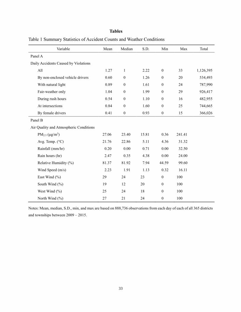
365 districts and townships from the 19 cities and counties in the main island of Taiwan. Panel A

of table 1 presents the selected summary statistics of daily accident counts in each district and

township. Among all accidents caused by driver violations, non-enclosed vehicle drivers were the

most liable for 47.45% of the accidents,13 69.95% occurred during times with ambient natural

light, 82.24% happened during fair-weather days (in contrast to cloudy, rainy, foggy, hazy, and

strong wind days), 42.88% in rush hours (7AM – 10AM and 5PM – 8PM), 66.11% at intersections,

and 32.49% with female drivers being the most liable party in the accidents.

The daily average air quality, measured by PM2.5 concentration, of each district and township

is calculated based on the spatial average from the 3km*3km grid-level data integrating hourly

13 Note that this highlights the representativeness of non-enclosed vehicle drivers of all drivers on the road in Taiwan.

11

ground level monitoring and long-term ground emission data from Taiwan EPA,14 satellite data of

aerosol optical depth (AOD) retrievals from MODerate resolution Imaging Spectroradiometer

(MODIS), and land use data from the National Land Surveying and Mapping Center.

An empirical challenge for many economic studies focusing on the (contemporaneous) effects

of air pollution is to obtain the air quality data at the same spatial resolution with outcome or other

key control variables. Many recent studies rely solely on ground monitoring data and use spatial

interpolation techniques, most commonly inverse distance weighting (e.g., Bondy et al. 2020,

Deryugina et al. 2019) and kriging (e.g., Burkhardt et al. 2019), to tackle the spatial sparsity of

ground monitoring stations. However, such spatial interpolation methods virtually ignore the roles

of terrain, land use, and ground emission. This problem is particularly relevant in our study because

of the highly heterogeneous landscapes and mountainous terrain in Taiwan (Jung et al. 2018). To

overcome this problem, we first build a linear mixed effect model that combines the 3km resolution

satellite-based AOD, land use, meteorological data to estimate PM2.5 concentrations with

comprehensive spatial coverage of Taiwan at the 3km*3km level. 15 The estimates are

subsequently validated by the ground monitoring data using a ten-fold cross validation and

multiple imputation with additive regression models to address the measurement error and

temporal missingness of satellite data.16 We therefore argue that our air quality data is also of

better quality than data that solely relies on satellite images. For more detail regarding the methods

14 The ground monitoring data are publicly available at the open data port of Taiwan EPA (https://data.epa.gov.tw/).

We retrieve the ground emission data from the Taiwan Emission Data System (TEDS 8.0 and 9.0 at

https://teds.epa.gov.tw/TEDS.aspx).

15 Some key land use categories are residential areas, industrial facilities, forest areas, farmlands, restaurants, shopping

centers, temples, roads, and bodies of water. Meteorological variables include temperature, relative humidity, surface

pressure, boundary layer height, and meridional and zonal winds.

16 A key issue of using satellite data to measure air quality in Taiwan is missing data due to cloud cover or high surface

reflection (Liu et al. 2016, Tsai et al. 2011).

12

used in constructing the grid air quality data, see Jung et al. (2018) and Wang et al. (2020).

We collect data on atmospheric conditions, including daily average temperature, total rain

hours, precipitation per hour, relative humidity, wind speed, and the number of hours that wind

blows from each of the directions from the Taiwan Air Quality Monitoring Network, hosted by the

Taiwan EPA. Panel B of table 1 reports the summary statistics of the key air pollutant, PM2.5, and

other weather variables included in the models. Figure 1 presents the average PM2.5 concentration

of each district and township in Taiwan during the study period. Air pollution is higher in the

western coastal plain areas and is lower in the central and eastern mountainous areas.

IV. Main Results

A. The Effects of Air Pollution on Accidents Caused by Risky Driving Behaviors

Table 2 summarizes the relationship between air pollution and accidents caused by violations,

using the fixed effects model specified in equation (1).17 In model 1 we regress the number of

accidents on PM2.5 concentration without controlling for any weather conditions or fixed effects,

and find a 1 μg/m3 increase in the daily average of PM2.5 concentration is associated with a 0.92%

increase in the number of accidents. We add weather controls, including the linear and squared

terms of daily average temperature, relative humidity, rainfall per hour, hours of rain, and wind

speed in model 2, and still find a significantly positive association between the number of accidents

and air pollution. As noted, these two models likely suffer from serious omitted variable biases,

because region-specific factors, especially traffic volume and population, can affect both accidents

caused by violations and air pollution.

In model 3, after region (district/township), year-by-month, and day-of-week fixed effects

17 Table A1 in the appendix presents the complete results, including the estimates of weather covariates.

13

being controlled for, we find a negative association, significant at the 0.1% level, between air

pollution and the number of accidents caused by violations. We deem that such a sign flip, after

adding the fixed effects, is a plausible outcome. A region with a higher population is likely to have

more traffic, traffic violations, accidents caused by violations, and a higher level of air pollution.18

Failure to control for region fixed effects will therefore bias the effect of air pollution on risky

driving behaviors upward. Similarly, higher traffic volume is potentially associated with more

traffic violations and worse air quality. Omitting those time-varying factors will again bias the

estimate upward. Still, this model may suffer from region-specific seasonal (year-by-month) and

periodic (day of week) correlations between air pollution and traffic patterns. Therefore, in model

4 we instead include region-by-year-by-month and region-by-day-of-week fixed effects, and find

a 1 μg/m3 increase in the daily average of PM2.5 is significantly associated with a 0.09% decrease

in the number of accidents caused by violations. As a robustness check, we conduct an OLS

estimation in model 5. We again find a significantly negative association, and the estimate is

quantitatively similar. Indicated by the implied semi-elasticity, a 1 μg/m3 increase in PM2.5 is

associated with a 0.12% decrease in the number of accidents caused by risky driving behaviors.

To further address other potential endogeneity issues, e.g., from any remaining unobserved

(region-specific) time-varying factors, reverse causality, and avoidance behaviors, we apply an

instrumental variable approach with a control function. The first stage results are reported in table

3.19 Regardless of the set of included instruments, the cluster-robust Kleibergen-Paap F statistics

show that wind directions are relevant instruments for PM2.5 concentration. We also find the effects

of each wind direction are largely in line with the atmospheric evidence. For example, north winds

18 Indeed, by regressing the number of accidents on population density, we find a 100-person increase in population

density per km2 is associated with a 0.71% increase in the number of accidents caused by violations.

19 Table A2 in the appendix presents the complete first-stage results, including the estimates of weather covariates.

14

move air pollutants to the downwind areas in the Southern air quality zone; and, with the mountain

ranges stretching from north to south and slightly aligning to the east, west winds lead to higher

levels of air pollution in the leeward-side Northern, Central, and Southern air quality zones.

We present the results using our IV strategy in table 4.20 Model 1 does not include weather

controls or fixed effects. With the air pollution being instrumented, we do not find any positive

association between air pollution and accidents caused by driver violations. Still, because wind

directions can affect many weather conditions such as temperature, precipitation, and humidity,

violating the exclusion restriction is certainly of our concern.

Models 2 and 3, arguably the most credible models for identifying the casual relationships of

our interests, yield virtually identical results. We find a 1 μg/m3 increase in PM2.5 is associated

with a 0.56 – 0.59% decrease in the number of accidents caused by risky driving behaviors, and

the estimates are both statistically significant at the 0.1% level. The K-P F-statistics show that wind

directions are relevant instruments. The exclusion restriction is likely to hold after controlling for

a host of weather covariates. Monotonicity is less of a concern when we allow the marginal effects

of wind directions on air pollutions to be air quality zone-specific. We also estimate the second

stage with OLS in model 4, and the implied semi-elasticity, -0.055, assures a robust result.

We thus far focus on the contemporaneous effect of air pollution on risky road behavior. Studies

have also found that some health outcomes response to cumulative exposure to air pollution (Tsai

et al. 2019). In model 5 we explore the cumulative (or lagged) effects of air pollution by including

PM2.5 concentrations in the three previous days. The results show that only same-day air pollution

has impacts on accidents caused by drivers’ risky behaviors. In the subsequent analyses, we use

the specification of model 3 (PPML with IV, weather controls, and region-specific temporal fixed

20 Table A3 in the appendix presents the complete estimation results, including the estimates of weather covariates.

15

effects) to conduct several robustness tests as well as to explore the nonlinear treatment effects and

transmission channels through which air pollution alters risky road behaviors.

B. Robustness Checks

We argue that our IV strategy has adequately addressed our primary identification issue

stemming from not including traffic volume. If the impacts of traffic volume had yet been treated

by our IV strategy, the effects of air pollution on accidents caused by drivers’ risky behaviors are

likely heterogeneous between time and locations with different traffic volumes or patterns. For

example, studies have documented that elevated air pollution decreases outdoor activities (e.g.,

Graff Zivin and Neidell 2009, Janke 2014, Saberian et al. 2017) and traffic from discretionary trips

(Cutter and Neidell 2009). If the effects of such avoidance behaviors on (non-commuting) traffic

volumes were still not accounted for by our instrument, we would expect to observe more negative

effects of air pollution on accidents caused by violations during times with higher shares of

discretionary trips (e.g., non-rush hours and weekends). To show that traffic volume no longer

poses a threat to our causal interpretations, we examine whether the effects of air pollution are

different for accidents that occurred in rush vs. non-rush hours, on weekdays vs. weekends, at

intersections or not, as well as in regions with different population densities.

Table 5 reports the results. Models 1 and 2 use the daily number of accidents occurred during

rush hours and non-rush hours as the outcome variable, respectively. Model 3 (model 4) uses the

sample from weekdays (weekends) only. Models 5 and 6 use the number of accidents that occurred

at an intersection and those not at an intersection, respectively. Model 7 (model 8) includes only

samples from regions with population densities lower than (higher than or equal to) the sample

median. We find the coefficients are all negative and similar in terms of magnitude. The results of

model 1 to 4 suggest that the negative effects of air pollution on accidents caused by violations are

16

unlikely explained by avoidance behaviors against air pollution. Indeed, we find the negative effect

in rush hours is even larger in magnitude than that in non-rush hours (-0.0068 vs. -0.0052).

Therefore, we conclude that our findings are not sensitive to, nor driven by, any remaining biases

from omitted traffic volume-related variables.21

We have demonstrated a pathway to infer the positive association between the level of air

pollution and individuals’ degree of risk aversion. Increased risk aversion and less risky driving

behaviors should have smaller effects on those accidents that are caused by mindless errors such

as failing to judge another vehicle’s path or speed. In model 9 we estimate the effect of air pollution

on the number of accidents caused by errors, according to the primary contributory factor and the

classification proposed by Reason et al. (1990). The effect, valued at -0.32%, is about half of that

on accidents caused by violations (-0.59% in model 3 in table 4) and is imprecisely estimated. This

result provides corroborating evidence for linking air pollution to the degree of risk aversion.22

In table A5 in the appendix, we report the estimation results using different specifications: (1)

including only the linear terms for the weather controls, (2) including eight separate wind

directions into as instruments, (3) including wind directions and speed as excluded instruments,23

21 We estimate several models to test if elevated air pollution would reduce traffic volumes using daily data from

Taipei City, the capital city of Taiwan. We do not find any evidence suggesting that air pollution would decrease traffic

volume. These results again indicate that avoidance behavior cannot explain the reduction in traffic accidents cause

by violations. The estimation results are presented in table A4 in the appendix.

22 We should note that we classified accidents being caused by mindless errors based on the contributory factors listed

in the accident reports conducted by polices. It is possible that some of these accidents are still caused by intended

aggressive driving behaviors, but that such behaviors are not caught by the polices. Therefore, reducing risky driving

behaviors can still reduce the number of accidents caused by errors, and this test is not completely a falsification

exercise.

23 Although wind speed has been used as an instrumental variable for air quality because of its relevance (e.g., He et

al. 2019), we believe that wind speed is not a valid instrument in our case because studies have documented its effect

on road safety (Dastoorpoor et al. 2016, Usman et al. 2012).

17

and (4) with daily observations aggregated at the spatially coarser county level to account for the

effect of a driver’s exposure to air pollution in regions other than the region where the accident

occurred. In addition, we estimate a model including only accidents occurred on sunny days with

good visibility, to minimize any potential effect from impaired visibility. All results are

quantitatively similar and support our key finding: elevated air pollution decreases the number of

accidents caused by driver violations.

Lastly, we acknowledge that our estimates still include the effects of air pollution on accidents

through other mechanisms such as impaired cognition, irritated respiratory systems, or increased

aggression.24 While a driver acts recklessly, impaired cognition or irritated respiratory organs due

to elevated air pollution can increase the likelihood of an accident. Therefore, the effect of air

pollution on reducing accidents through increased risk aversion is likely to be even larger when

other effects are isolated. We more formally address this issue in the nonlinear effect of air

pollution later.

V. Transmission Channels, Nonlinearity, and Heterogenous Treatment Effects

A. The Transmission Channels of Air Pollution Affecting Risky Driving Behaviors

Air pollution can affect mood and behaviors, including increased risk aversion, through both

respiratory and visual channels. To shed light on the transmission channels through which air

pollution affects driver behaviors and the resulting accidents, we explore the heterogeneous effects

of air pollution (1) on drivers with different levels of direct exposure to air pollution and (2) under

conditions whether air quality can be visually assessed. In light of our key findings and the credible

evidence showing that non-enclosed vehicle drivers should on average have a much higher level

24 The mechanism of increased aggression is suggested by a few recent studies on the positive association between

air pollution and crime (Bondy et al. 2020, Burkhardt et al. 2019, Herrnstadt et al. forthcoming).

18

of exposure to air pollution through their respiratory systems than drivers of enclosed vehicle do,

we first hypothesize that air pollution would reduce the number of accidents primarily caused by

violations committed by non-enclosed vehicle drivers more than those by enclosed vehicle

drivers.25

Models 1 and 2 of table 6 present the results of the effects of air pollution on the number of

accidents caused by violations committed by drivers of enclosed and non-enclosed vehicles,

respectively.26 The estimated effect on accidents caused by violations of non-enclosed vehicle

drivers is only slightly more negative than that of enclosed vehicle drivers (-0.67% vs. -0.57%).

Therefore, we find little evidence to show that air pollution affects road users’ risky behaviors

through the respiratory system.27

Subsequently, we explore whether air quality can affect risky driving behaviors through visual

channels. As noted, it is much easier to assess air quality when there is natural light (Hyslop 2009,

Yu et al. 2018). Therefore, we hypothesize that the effect would be stronger during times with

ambient natural light than during times without. Models 3 and 4 in table 6 present the estimation

25 Sager (2019) conducted a similar investigation and expected that air pollution would have a stronger effect on

increasing the number of non-enclosed vehicles involved in accidents than on enclosed vehicles. However, he finds

that the positive effect is smaller on non-enclosed vehicles but provides no explanation. Our proposed hypothesis can

therefore provide a coherent justification for this particularly puzzled result in Sager’s study.

26 We exclude the very small number of accidents principally caused by pedestrians’ violations.

27 It is possible that non-enclosed vehicle drivers perform defense health behaviors such as wearing masks. However,

we are not aware of any evidence indicating a large share of non-enclosed vehicle drivers regularly wearing masks

that can effectively filter out PM2.5, the air pollutant that our study focuses on. On the other hand, enclosed vehicle

drivers, if they keep the windows open, might still expose to similar levels of air pollution to those among non-

enclosed vehicle drivers. However, with nearly all enclosed vehicles equipped with air condition and the hot and rainy

subtropical climate in Taiwan, it is uncommon for enclosed vehicle drivers to have their windows open, especially in

populated areas. We therefore believe that these unobserved behaviors are unlikely to close the gap in direct air

pollution exposure between enclosed and non-enclosed vehicle drivers, which has been well documented in the

literature (Dirks et al. 2012, Rivas et al. 2017, Tsai et al. 2008, Vlachokostas et al. 2012).

19

results. We find that a 1 μg/m3 increase in PM2.5 leads to a 0.79% decrease in the number of

accidents caused by risky driving behaviors when there is natural light. However, the effect of a 1

μg/m3 increase in PM2.5 is much smaller (-0.18%) and is imprecisely estimated in time without

natural light. As a placebo test, we use the same IV specification to examine the effect of ozone,

which is generally found to have little impact on the haziness of skies (Liu et al. 2020), on accidents

caused violations. The results show an insignificant and slightly positive effect of ozone on

accidents (see table A6 in the appendix). We therefore find strong evidence to demonstrate that air

quality can affect risky driving behaviors through visual channels and infer that a person’s degree

of risk aversion can increase simply by “seeing” air pollution (i.e. when the skies are hazy).

B. Nonlinear and Heterogeneous Treatment Effects

Medical literature has shown that the dose-response relationships between air pollution and

health outcomes can be nonlinear (e.g., Daniels et al. 2000, Dominici et al. 2002). Several

economic studies have also found nonlinear effects of air pollution on various societal outcomes,

e.g., Burkhardt et al. (2019) on crime, Ebenstein et al. (2016) on life expectancy, and Schlenker

and Walker (2016) on hospitalization costs. We are not aware of any exploration of the nonlinearity

in the effect of air pollution on risk attitude or risky behaviors. We subsequently examine whether

such nonlinearity exists.

Based on each region’s average PM2.5 concentration, we stratify all regions into two groups

(the better and worse 50) using the sample median of daily average PM2.5 concentration of the

entire study period as the cutoff. Models 1 and 2 in table 7 present the estimation results from the

models using these two subsamples, respectively. We find the negative effect of air pollution on

the number of accidents caused by violations is only significant in the worse 50 regions with higher

level of air pollution, and the effect size is more than doubled of that in the regions with better air

20

quality (-0.62% vs. -0.26%). The average PM2.5 concentration in the data of Sager (2019) is 13.32

μg/m3, and he finds a 1 μg/m3 increase in PM2.5 is associated with 0.3 – 0.6% more accidents. The

average PM2.5 concentration in our top and bottom halves of the regions are 20.42 and 33.56

μg/m3, respectively. Interestingly, by combining the two estimates from our study and that from

Sager (2019), we observe the effect of air pollution on road accidents monotonically decreases

with higher level of air pollution.

We further leverage control function’s ability to deal with the nonlinearity in the endogenous

variable in the second stage and include linear splines of PM2.5 concentration in model 3

(Henderson and Souto 2018, Wooldridge 2015). We find a positive, albeit insignificant, effect of

air pollution on accidents when the PM2.5 concentration is below or equal to 10 μg/m3, and only

identify the negative effects when the PM2.5 concentration is above 10 μg/m3. This result provides

corroborating evidence of the nonlinearity in the effect of air pollution on risky road behaviors.

These results suggest that the marginal effect of air pollution on reducing accidents through

increased risk aversion rises more quickly than the effect on increasing accidents through impaired

cognition (or irritated respiratory systems) with elevated air pollution levels. We illustrate such

relationships conceptually in figure 2. The dotted line shows the total (accumulated) effect size of

air pollution on decreasing accidents through increased levels of risk aversion, and the dashed line

shows the effect on increasing accidents through cognitive impairment. The solid line represents

the combined marginal effect, which is the difference between the accumulated effect from

increased risk aversion and that from cognitive impairment. Our data and analyses have recovered

the marginal effect when air pollution is relatively high, for example, the shaded area (I), where

the size of the accumulated effect of increased risk aversion is larger than that of cognitive

impairment. The results in Sager (2019), on the other hand, may have traced out the positive

21

marginal effect of air pollution on accidents in area (II).28 This illustration not only highlights the

nonlinear effect of air pollution on risky aversion or impaired cognition, but shows that our results

can actually be “consistent” with those from Sager.29

Many studies have found that gender and age are two of the key characteristics for explaining

an individual’s risk tolerance (e.g., Borghans et al. 2009, Halek and Eisenhauer 2001, Hartog et al.

2002). We examine whether the effects of air pollution on risky road behaviors are heterogeneous

across gender and age groups. Table 8 presents the associated results. In models 1 and 2, the

outcome variables are the number of accidents caused by violations for which a female or male

driver is primarily liable. The effects are virtually identical. Therefore, we do not find evidence to

show that air pollution heterogeneously influences drivers of different biological gender.

In models 3 to 5, we use the counts of the most liable driver in an accident by age groups

(below 40, 40 to 64, and 65 and above) as the outcome variables. We find the effects to be largely

homogeneous across the two younger groups (-0.61% and -0.62%). However, the effect on the

number of accidents primarily caused by violations committed by drivers 65 years old and above

is much lower (-0.34%) and imprecisely estimated.30 Corroborating with the results showing

28 Moreover, our model that includes the linear splines of air pollution, model (3) in table 7, provides indicative

evidence of the shape of the entire solid curve. Despite the insignificant positive effect when PM2.5 concentration is

below 10 μg/m3, the model suggests that the net marginal effect equals to zero when PM2.5 concentration is 18.22

μg/m3, which is in line with the estimates at different average levels of air pollution from our study (model 1 and 2 in

table 7) and those from Sager (2019). Still, we note that the estimates of ours and those of Sager (2019) are not

necessarily comparable, given that we primarily focus on accidents caused on violations and the traffic conditions and

dynamics are likely very different between Taiwan and the U.K.

29 Although our example depicts both of the dose-response relationships being nonlinear, we can recover a similar

combined marginal effect of air pollution on accidents as long as one of the dose-responses is nonlinear, assuming

there is no effect of air pollution on cognition nor risk aversion when the level of ai pollution is zero.

30 Trips of those 65 years old and above are more likely discretionary. Therefore, the smaller negative effect of air

pollution among elderlies once again suggest that avoidance behaviors against air pollution cannot explain the

reduction in accidents.

22

nonlinear effects, this heterogeneity suggests that the effect on cognition may be relatively stronger,

compared to the effect on risk aversion, among elderly drivers. This can be illustrated by an upward

shift of the effect of air pollution on cognition (the dashed line) in figure 2, while holding the effect

of air pollution on risk aversion (the dotted line).31

VI. Conclusion and Discussion

Despite a large strand of literature on the socio-economic costs of air pollution, in this study

we find a rare “benefit” of air pollution: reducing accidents caused by risky behaviors on roads.

Using administrative traffic accident records and high-resolution air quality data of Taiwan, we

identify air quality as a new factor for changing life-threatening risky behaviors. Our results find

that elevated air pollution, measured by PM2.5 concentration, leads to fewer traffic accidents caused

by driver violations, but has no significant effect on those caused by mindless errors. Specifically,

we find that a 1 μg/m3 increase in PM2.5 concentration leads to a 0.59% decrease in accidents

caused by driver violations. That is, a one-standard deviation increases in PM2.5 concentration can

decrease such accidents by more than 9%. In addition, the nonlinearity in the dose-response

relationship between air pollution and accidents suggest that, among the effects of air pollution on

risk aversion and cognition, at least one of them is nonlinear. These results in particular add to the

literature on the determinants of risky behaviors (Dohmen et al. 2011) and (non)stability of risk

preferences (Schildberg-Hörisch 2018)

Cognitive ability and risk tolerance have been shown to be interrelated in determining many

31 Elderlies are in general more risk averse (Halek and Eisenhauer 2001, Hartog et al. 2002), so another natural

explanation for the heterogeneity across age groups is that air pollution has a smaller effect on risky behaviors among

those who are more risk averse. However, since females are on average more risk averse, the homogeneous effects

across genders do not support such explanation.

23

economic outcomes such as investment in human capital and inequality (Dohmen et al. 2018,

Heckman et al. 2006). Our results by no means lead us to advocate for less stringent air pollution

regulation, nor do they suggest that the costs of air pollution have been overestimated. Instead,

given that the effects of air pollution on risk aversion and impaired cognition (and irritated

respiratory systems) can influence risky behaviors in the opposite directions, the estimated cost of

air pollution on cognitive performance and other associated health outcomes involving risk

attitudes may be underestimated, if the effect on risk attitudes is not isolated.32

We further find such negative effects are only observed in times when air quality can be

visually assessed, i.e., when natural light is available. However, the effect is largely homogeneous

across the drivers of enclosed and non-enclosed vehicle, who arguably are exposed to very

different levels of air pollution. These results show that air quality can affect risky driving

behaviors through visual channels, but there is no evidence to validate the respiratory route. To the

best of our knowledge, we are the first economic study that is able to simultaneously test these two

transmission channels. This finding also implies that, when quantifying the effects of different air

pollutants on societal outcomes, one should pay attention to how the focused pollutants can change

an individual’s visual perception of the environment. For example, ozone in general has small

impact on visibility and can even makes the sky bluer, which is visually pleasant to many; therefore,

ozone may simultaneously weaken cognitive performance and reduce risk aversion. Failure to

32 For example, He et al. (2019) find that air pollution decreases the productivity of call center workers, primarily

through an increase in breaks. For some jobs, without precise measures of output, taking more breaks could be directly

considered to reflect lower productivity and risks one’s job security. A worker with a higher level of risk aversion

might refrain from taking breaks. Such behavior would mitigate some observable losses in productivity due to elevated

air pollution. On the other hand, if lower level of risk tolerance makes an individual who feels ill more likely to seek

a consultation of a physician, failure to isolate the effect of risk preferences may lead to overestimation of the cost of

air pollution measured by medical expenditure.

24

isolate one effect from the other, again, may prejudice the casual interpretation of the estimated

effects of ozone pollution.

Some might see our key finding—elevated air pollution decreases accidents caused by risky

driving behaviors—surprising and even in stark contrast to common wisdom like the results in

Sager (2019), who used a similar research design but focused on all types of traffic accidents in

the United Kingdom. Indeed, we find no significant effect of air pollution on traffic accidents

caused by harmless lapses nor those caused by violations in areas with more comparable air quality

to that in highly developed countries. Our results show a nonlinear dose-response relationship

between air pollution and risky behaviors on roads. That is, air pollution likely increases the degree

of risk aversion at an increasing rate or at least at a rate faster than that on reducing cognition.

Corroborating our results with those from Sager (2019) enhances the external validity of the

estimated effects of air pollution on road safety and risky behaviors in general. Our empirical

results have more direct implications and are more readily transferable to many non-high-income

countries, where the climates, environmental quality, and traffic compositions are more similar to

those in Taiwan. Moreover, the nonlinearity in air pollution dose-response reinforces the

motivation for investigating the distributional effects of air pollution across groups with different

levels of exposure (Hsiang et al. 2019). Exploring the nonlinear effects of air pollution on different

risky behaviors or direct measures of risk aversion is an interesting avenue for future work. Lastly,

another straightforward extension will be to investigate the effects of air pollution on more

common outcomes of risky driving behaviors such as traffic violations, especially speeding caught

by enforcement cameras.

25

References

Anderson, M. L. (2020). As the wind blows: The effects of long-term exposure to air pollution

on mortality. Journal of the European Economic Association, 18(4), 1886-1927.

Anstey, K. J., Horswill, M. S., Wood, J. M., & Hatherly, C. (2012). The role of cognitive and

visual abilities as predictors in the multifactorial model of driving safety. Accident Analysis

& Prevention, 45, 766-774.

Arceo, E., Hanna, R., & Oliva, P. (2016). Does the effect of pollution on infant mortality differ

between developing and developed countries? Evidence from Mexico City. The Economic

Journal, 126(591), 257-280.

Archsmith, J., Heyes, A., & Saberian, S. (2018). Air quality and error quantity: Pollution and

performance in a high-skilled, quality-focused occupation. Journal of the Association of

Environmental and Resource Economists, 5(4), 827-863.

Bassi, A., Colacito, R., & Fulghieri, P. (2013). ’O sole mio: An experimental analysis of weather

and risk attitudes in financial decisions. The Review of Financial Studies, 26(7), 1824-1852.

Bedi, A. S., Nakaguma, M. Y., Restrepo, B. J., & Rieger, M. (2021). Particle pollution and

cognition: Evidence from sensitive cognitive tests in Brazil. Journal of the Association of

Environmental and Resource Economists, 8(3), 443-474.

Blundell, R., & Powell, J. L. (2003). Endogeneity in nonparametric and semiparametric

regression models. In Advances in Economics and Econonometrics: Theory and

Applications, Eighth World Congress, Volume 2, ed. Mathias Dewatripont, Lars Hansen, and

Stephen Turnovsky, 312–57. Cambridge: Cambridge University Press

Bondy, M., Roth, S., & Sager, L. (2020). Crime is in the air: The contemporaneous relationship

between air pollution and crime. Journal of the Association of Environmental and Resource

Economists, 7(3), 555-585.

Borghans, L., Heckman, J. J., Golsteyn, B. H., & Meijers, H. (2009). Gender differences in risk

aversion and ambiguity aversion. Journal of the European Economic Association, 7(2-3),

649-658.

Brijs, T., Karlis, D., & Wets, G. (2008). Studying the effect of weather conditions on daily crash

counts using a discrete time-series model. Accident Analysis & Prevention, 40(3), 1180-

1190.

Brimblecombe, P. (1987). The Big Smoke: A History of Air Pollution in London since Medieval

Times. Routledge.

26

Brook, R. D., Brook, J. R., Urch, B., Vincent, R., Rajagopalan, S., & Silverman, F. (2002).

Inhalation of fine particulate air pollution and ozone causes acute arterial vasoconstriction in

healthy adults. Circulation, 105(13), 1534-1536.

Burkhardt, J., Bayham, J., Wilson, A., Carter, E., Berman, J. D., O'Dell, K., ... & Pierce, J. R.

(2019). The effect of pollution on crime: Evidence from data on particulate matter and

ozone. Journal of Environmental Economics and Management, 98, 102267.

Caliendo, C., Guida, M., & Parisi, A. (2007). A crash-prediction model for multilane roads.

Accident Analysis & Prevention, 39(4), 657-670.

Carneiro, J., Cole, M., & Strobl, E. (2021). The effects of air pollution on students' cognitive

performance: Evidence from Brazilian university entrance tests. Journal of the Association

of Environmental and Resource Economists, 8(6), 1051-1077.

Chang, T. Y., Graff Zivin, J., Gross, T., & Neidell, M. (2019). The effect of pollution on worker

productivity: evidence from call center workers in China. American Economic Journal:

Applied Economics, 11(1), 151-72.

Chew, S. H., Huang, W., & Li, X. (2021). Does haze cloud decision making? A natural laboratory

experiment. Journal of Economic Behavior & Organization, 182, 132-161.

Coates, J. M., & Herbert, J. (2008). Endogenous steroids and financial risk taking on a London

trading floor. Proceedings of the National Academy of Sciences, 105(16), 6167-6172.

Correia, S., Guimarães, P., & Zylkin, T. (2020). Fast Poisson estimation with high-dimensional

fixed effects. The Stata Journal, 20(1), 95-115.

Currie, J., & Walker, R. (2019). What do economists have to say about the Clean Air Act 50

years after the establishment of the Environmental Protection Agency? Journal of Economic

Perspectives, 33(4), 3-26.

Cutter, W. B., & Neidell, M. (2009). Voluntary information programs and environmental

regulation: Evidence from ‘Spare the Air’. Journal of Environmental Economics and

Management, 58(3), 253-265.

Daniels, M. J., Dominici, F., Samet, J. M., & Zeger, S. L. (2000). Estimating particulate matter-

mortality dose-response curves and threshold levels: an analysis of daily time-series for the

20 largest US cities. American Journal of Epidemiology, 152(5), 397-406.

Dastoorpoor, M., Idani, E., Khanjani, N., Goudarzi, G., & Bahrampour, A. (2016). Relationship

between air pollution, Weather, traffic, and traffic-related mortality. Trauma Monthly, 21(4).

Deryugina, T., Heutel, G., Miller, N. H., Molitor, D., & Reif, J. (2019). The mortality and

27

medical costs of air pollution: Evidence from changes in wind direction. American

Economic Review, 109(12), 4178-4219.

Dirks, K., Sharma, P., A Salmond, J., & B Costello, S. (2012). Personal exposure to air pollution

for various modes of transport in Auckland, New Zealand. The Open Atmospheric Science

Journal, 6(1).

Dohmen, T., Falk, A., Huffman, D., & Sunde, U. (2010). Are risk aversion and impatience

related to cognitive ability? American Economic Review, 100(3), 1238-60.

Dohmen, T., Falk, A., Huffman, D., & Sunde, U. (2018). On the relationship between cognitive

ability and risk preference. Journal of Economic Perspectives, 32(2), 115-34.

Dohmen, T., Falk, A., Huffman, D., Sunde, U., Schupp, J., & Wagner, G. G. (2011). Individual

risk attitudes: Measurement, determinants, and behavioral consequences. Journal of the

European Economic Association, 9(3), 522-550.

Dominici, F., Daniels, M., Zeger, S. L., & Samet, J. M. (2002). Air pollution and mortality:

estimating regional and national dose-response relationships. Journal of the American

Statistical Association, 97(457), 100-111.

Dong, R., Fisman, R., Wang, Y., & Xu, N. (2021). Air pollution, affect, and forecasting bias:

Evidence from Chinese financial analysts. Journal of Financial Economics, 139, 971-984.

Ebenstein, A., Fan, M., Greenstone, M., He, G., & Zhou, M. (2017). New evidence on the impact

of sustained exposure to air pollution on life expectancy from China’s Huai River

Policy. Proceedings of the National Academy of Sciences, 114(39), 10384-10389.

Goetzmann, W. N., Kim, D., Kumar, A., & Wang, Q. (2015). Weather-induced mood,

institutional investors, and stock returns. The Review of Financial Studies, 28(1), 73-111.

Graff Zivin, J., & Neidell, M. (2009). Days of haze: Environmental information disclosure and

intertemporal avoidance behavior. Journal of Environmental Economics and

Management, 58(2), 119-128.

Graff Zivin, J., & Neidell, M. (2012). The impact of pollution on worker productivity. American

Economic Review, 102(7), 3652-73.

Green, C. P., Heywood, J. S., & Navarro, M. (2016). Traffic accidents and the London

congestion charge. Journal of Public Economics, 133, 11-22.

Gurgueira, S. A., Lawrence, J., Coull, B., Murthy, G. K., & González-Flecha, B. (2002). Rapid

increases in the steady-state concentration of reactive oxygen species in the lungs and heart

after particulate air pollution inhalation. Environmental Health Perspectives, 110(8), 749-

28

755.

Halek, M., & Eisenhauer, J. G. (2001). Demography of risk aversion. Journal of Risk and

Insurance, 1-24.

Hartog, J., Ferrer‐i‐Carbonell, A., & Jonker, N. (2002). Linking measured risk aversion to

individual characteristics. Kyklos, 55(1), 3-26.

He, J., Liu, H., & Salvo, A. (2019). Severe air pollution and labor productivity: Evidence from

industrial towns in China. American Economic Journal: Applied Economics, 11(1), 173-201.

Heckman, J. J., Stixrud, J., & Urzua, S. (2006). The effects of cognitive and noncognitive

abilities on labor market outcomes and social behavior. Journal of Labor economics, 24(3),

411-482.

Heissel, J. A., Persico, C. L., & Simon, D. (2020). Does pollution drive achievement? The effect

of traffic pollution on academic performance. Journal of Human Resources, 1218-9903R2.

Henderson, D. J., & Souto, A. C. (2018). An introduction to nonparametric regression for labor

economists. Journal of Labor Research, 39(4), 355-382.

Herrnstadt, E., Heyes, A., Muehlegger, E., & Saberian, S. (Forthcoming). Air pollution and

criminal activity: Microgeographic evidence from Chicago. American Economic Journal:

Applied Economics.

Heyes, A., Neidell, M., & Saberian, S. (2016). The effect of air pollution on investor behavior:

Evidence from the S&P 500. NBER Working Paper, 22753.

Hirshleifer, D., & Shumway, T. (2003). Good day sunshine: Stock returns and the weather. The

Journal of Finance, 58(3), 1009-1032.

Huang, R. J., Zhang, Y., Bozzetti, C., Ho, K. F., Cao, J. J., Han, Y., ... & Prévôt, A. S. (2014).

High secondary aerosol contribution to particulate pollution during haze events in

China. Nature, 514(7521), 218-222.

Hsiang, S., Oliva, P., & Walker, R. (2019). The distribution of environmental damages. Review of

Environmental Economics and Policy, 13(1), 83-103.

Hyslop, N. P. (2009). Impaired visibility: The air pollution people see. Atmospheric

Environment, 43(1), 182-195.

Janke, K. (2014). Air pollution, avoidance behaviour and children's respiratory health: Evidence

from England. Journal of Health Economics, 38, 23-42.

Jung, C. R., Hwang, B. F., & Chen, W. T. (2018). Incorporating long-term satellite-based aerosol

optical depth, localized land use data, and meteorological variables to estimate ground-level

29

PM2.5 concentrations in Taiwan from 2005 to 2015. Environmental Pollution, 237, 1000-

1010.

Kandasamy, N., Hardy, B., Page, L., Schaffner, M., Graggaber, J., Powlson, A. S., Fletcher, P. C.,

Gurnell, M., & Coates, J. (2014). Cortisol shifts financial risk preferences. Proceedings of

the National Academy of Sciences, 111(9), 3608-3613.

Kliger, D., & Levy, O. (2003). Mood-induced variation in risk preferences. Journal of Economic

Behavior & Organization, 52(4), 573-584.

Knittel, C. R., Miller, D. L., & Sanders, N. J. (2016). Caution, drivers! Children present: Traffic,

pollution, and infant health. Review of Economics and Statistics, 98(2), 350-366.

Lai, W., Li, S., Li, Y., & Tian, X. (2021). Air Pollution and Cognitive Functions: Evidence from

Straw Burning in China. American Journal of Agricultural Economics.

doi:10.1111/ajae.12225

Levy, T., & Yagil, J. (2011). Air pollution and stock returns in the US. Journal of Economic

Psychology, 32(3), 374-383.

Li, H., Cai, J., Chen, R., Zhao, Z., Ying, Z., Wang, L., Chen, J., Hao, K., Kinney, P. L., & Chen,

H. (2017). Particulate matter exposure and stress hormone levels: a randomized, double-

blind, crossover trial of air purification. Circulation, 136(7), 618-627.

Li, J. J., Massa, M., Zhang, H., & Zhang, J. (2019). Air pollution, behavioral bias, and the

disposition effect in China. Journal of Financial Economics.

Lichter, A., Pestel, N., & Sommer, E. (2017). Productivity effects of air pollution: Evidence from

professional soccer. Labour Economics, 48, 54-66.

Liou, Y-A., Yan, S-K., & Yang, Z-Y. (2004) Thermal inversion in Taiwan. The 8th Annual

Conference of Atmospheric Science.

Liu, C. J., Liu, C. Y., Mong, N. T., & Chou, C. C. (2016). Spatial correlation of satellite-derived

PM2. 5 with hospital admissions for respiratory diseases. Remote Sensing, 8(11), 914.

Liu, J., Ren, C., Huang, X., Nie, W., Wang, J., Sun, P., Chi, X. & Ding, A. (2020). Increased

aerosol extinction efficiency hinders visibility improvement in eastern China. Geophysical

Research Letters, 47(20), e2020GL090167.

Lu, J. G., Lee, J. J., Gino, F., & Galinsky, A. D. (2018). Polluted morality: Air pollution predicts

criminal activity and unethical behavior. Psychological Science, 29(3), 340-355.

Maurer, M., Klemm, O., Lokys, H. L., & Lin, N. H. (2019). Trends of fog and visibility in

Taiwan: climate change or air quality improvement? Aerosol and Air Quality

30

Research, 19(4), 896-910.

Middleton, P., Stewart, T. R., & Leary, J. (1985). On the use of human judgment and

physical/chemical measurements in visual air quality management. Journal of the Air

Pollution Control Association, 35(1), 11-18.

Moretti, E., & Neidell, M. (2011). Pollution, health, and avoidance behavior evidence from the

ports of Los Angeles. Journal of Human Resources, 46(1), 154-175.

Neidell, M. (2009). Information, avoidance behavior, and health the effect of ozone on asthma

hospitalizations. Journal of Human Resources, 44(2), 450-478.

Ouimette, J. R., & Flagan, R. C. (1982). The extinction coefficient of multicomponent

aerosols. Atmospheric Environment (1967), 16(10), 2405-2419.

Pasidis, I. (2017). Congestion by accident? A two-way relationship for highways in

England. Journal of Transport Geography.

Persico, C. L., & Venator, J. (2021). The effects of local industrial pollution on students and

schools. Journal of Human Resources, 56(2), 406-445.

Quddus, M. A., Wang, C., & Ison, S. G. (2009). Road traffic congestion and crash severity:

econometric analysis using ordered response models. Journal of Transportation

Engineering, 136(5), 424-435.

Reason, J., Manstead, A., Stradling, S., Baxter, J., & Campbell, K. (1990). Errors and violations

on the roads: a real distinction? Ergonomics, 33(10-11), 1315-1332.

Rivas, I., Kumar, P., & Hagen-Zanker, A. (2017). Exposure to air pollutants during commuting in

London: are there inequalities among different socio-economic groups? Environment

International, 101, 143-157.

Rosenblitt, J. C., Soler, H., Johnson, S. E., & Quadagno, D. M. (2001). Sensation seeking and

hormones in men and women: exploring the link. Hormones and Behavior, 40(3), 396-402.

Saberian, S., Heyes, A., & Rivers, N. (2017). Alerts work! Air quality warnings and

cycling. Resource and Energy Economics, 49, 165-185.

Sager, L. (2019). Estimating the effect of air pollution on road safety using atmospheric

temperature inversions. Journal of Environmental Economics and Management, 98, 102250.

Saunders, E. M. (1993). Stock prices and Wall Street weather. The American Economic Review,

83(5), 1337-1345.

Schildberg-Hörisch, H. (2018). Are risk preferences stable? Journal of Economic

Perspectives, 32(2), 135-54.

31

Schlenker, W., & Walker, W. R. (2016). Airports, air pollution, and contemporaneous health. The

Review of Economic Studies, 83(2), 768-809.

Schmidt, S. (2019). Brain fog: Does air pollution make us less productive? Environmental

Health Perspectives, 127(5), 52001.

Schoemaker, P. J. (1993). Determinants of risk-taking: Behavioral and economic views. Journal

of Risk and Uncertainty, 6(1), 49-73.

Schultheis, M. T., Garay, E., & DeLuca, J. (2001). The influence of cognitive impairment on

driving performance in multiple sclerosis. Neurology, 56(8), 1089-1094.

Shie, R.-H., Lee, J.-H., & Chan, C.-C. (2016). Temporal-Spatial Distribution of PM2.5

Concentration and the Contribution of Sources in Taiwan. Formosan Journal of

Medicine, 20(4), 367-376.

Shr, Y-H., P-J. Chang, T-C. Hsiao (2021) Assessing the benefits of air quality improvement

programs through citizen perception and monitoring data. Final Report to Air Pollution

Mitigation Fund Research Grant. Taiwan Environmental Protection Agency.

Silva, J. S., & Tenreyro, S. (2006). The log of gravity. The Review of Economics and Statistics,

88(4), 641-658.

Taiwan EPA (2017) Measuring the exposure to air pollutants among commuters in Taipei (臺北

都會區通勤期間之空氣污染物暴露量調查). Taiwan Environmental Protection Agency

Research Report.

Tao, Y., Kollios, G., Considine, J., Li, F., & Papadias, D. (2004). Spatio-temporal aggregation

using sketches. In Proceedings. 20th International Conference on Data Engineering (pp.

214-225). IEEE.

Tsai, D. H., Wu, Y. H., & Chan, C. C. (2008). Comparisons of commuter's exposure to particulate

matters while using different transportation modes. Science of the Total Environment, 405(1-

3), 71-77.

Tsai, T. C., Jeng, Y. J., Chu, D. A., Chen, J. P., & Chang, S. C. (2011). Analysis of the

relationship between MODIS aerosol optical depth and particulate matter from 2006 to

2008. Atmospheric Environment, 45(27), 4777-4788.

Tsai, T. L., Lin, Y. T., Hwang, B. F., Nakayama, S. F., Tsai, C. H., Sun, X. L., ... & Jung, C. R.

(2019). Fine particulate matter is a potential determinant of Alzheimer's disease: A systemic

review and meta-analysis. Environmental Research, 177, 108638.

Usman, T., Fu, L., & Miranda-Moreno, L. F. (2012). A disaggregate model for quantifying the

32

safety effects of winter road maintenance activities at an operational level. Accident Analysis

& Prevention, 48, 368-378.

Van Brussel, S., & Huyse, H. (2019). Citizen science on speed? Realising the triple objective of

scientific rigour, policy influence and deep citizen engagement in a large-scale citizen

science project on ambient air quality in Antwerp. Journal of Environmental Planning and

Management, 62(3), 534-551.

Vlachokostas, C., Achillas, C., Michailidou, A. V., & Moussiopoulos, Ν. (2012). Measuring

combined exposure to environmental pressures in urban areas: An air quality and noise

pollution assessment approach. Environment International, 39(1), 8-18.

Wan, Y., Li, Y., Liu, C., & Li, Z. (2020). Is traffic accident related to air pollution? A case report

from an island of Taihu Lake, China. Atmospheric Pollution Research, 11(5), 1028-1033.

Wang, C. M., Jung, C. R., Chen, W. T., & Hwang, B. F. (2020). Exposure to fine particulate

matter (PM2. 5) and pediatric rheumatic diseases. Environment International, 138, 105602.

Wooldridge, J. M. (2015). Control function methods in applied econometrics. Journal of Human

Resources, 50(2), 420-445.

World Health Organization (2018) Global Status Report on Road Safety 2018. Geneva. Licence:

CC BYNC-SA 3.0 IGO.

Yu, Y., Zhao, C., Kuang, Y., Tao, J., Zhao, G., Shen, C., & Xu, W. (2018). A parameterization for

the light scattering enhancement factor with aerosol chemical compositions. Atmospheric

Environment, 191, 370-377.

Zhou, M., & Sisiopiku, V. P. (1997). Relationship between volume-to-capacity ratios and

accident rates. Transportation Research Record, 1581(1), 47-52.

33

Tables

Table 1 Summary Statistics of Accident Counts and Weather Conditions

Variable Mean Median S.D. Min Max Total

Panel A

Daily Accidents Caused by Violations

All 1.27 1 2.22 0 33 1,126,395

By non-enclosed vehicle drivers 0.60 0 1.26 0 20 534,493

With natural light 0.89 0 1.61 0 24 787,990

Fair-weather only 1.04 0 1.99 0 29 926,417

During rush hours 0.54 0 1.10 0 16 482,955

At intersections 0.84 0 1.60 0 25 744,665

By female drivers 0.41 0 0.93 0 15 366,026

Panel B

Air Quality and Atmospheric Conditions

PM2.5 (μg/m3) 27.06 23.40 15.81 0.36 241.41

Avg. Temp. (°C) 21.76 22.86 5.11 4.36 31.32

Rainfall (mm/hr) 0.20 0.00 0.71 0.00 32.50

Rain hours (hr) 2.47 0.35 4.38 0.00 24.00

Relative Humidity (%) 81.37 81.92 7.94 44.59 99.60

Wind Speed (m/s) 2.23 1.91 1.13 0.32 16.11

East Wind (%) 29 24 23 0 100

South Wind (%) 19 12 20 0 100

West Wind (%) 25 24 18 0 100

North Wind (%) 27 21 24 0 100

Notes: Mean, median, S.D., min, and max are based on 888,736 observations from each day of each of all 365 districts

and townships between 2009 – 2015.

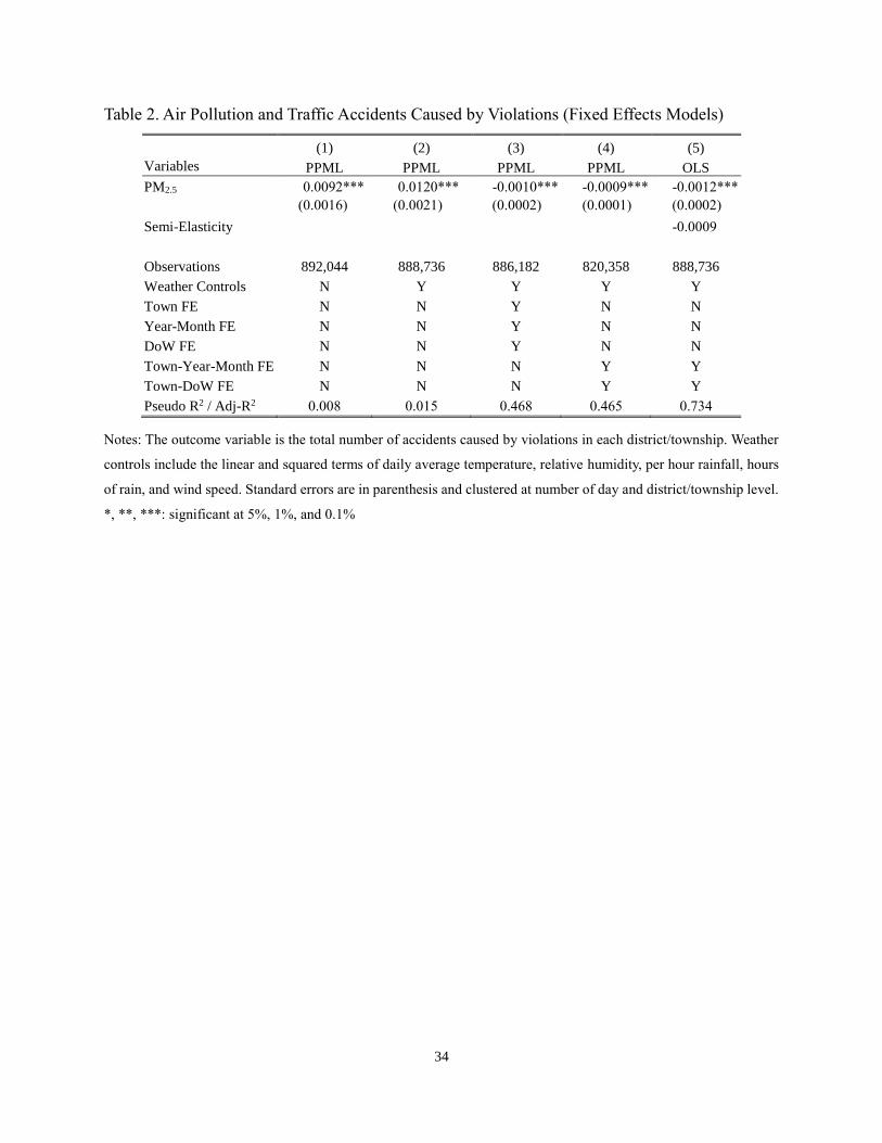
34

Table 2. Air Pollution and Traffic Accidents Caused by Violations (Fixed Effects Models)

(1) (2) (3) (4) (5)

Variables PPML PPML PPML PPML OLS

PM2.5 0.0092*** 0.0120*** -0.0010*** -0.0009*** -0.0012***

(0.0016) (0.0021) (0.0002) (0.0001) (0.0002)

Semi-Elasticity -0.0009

Observations 892,044 888,736 886,182 820,358 888,736

Weather Controls N Y Y Y Y

Town FE N N Y N N

Year-Month FE N N Y N N

DoW FE N N Y N N

Town-Year-Month FE N N N Y Y

Town-DoW FE N N N Y Y

Pseudo R2 / Adj-R2 0.008 0.015 0.468 0.465 0.734

Notes: The outcome variable is the total number of accidents caused by violations in each district/township. Weather

controls include the linear and squared terms of daily average temperature, relative humidity, per hour rainfall, hours

of rain, and wind speed. Standard errors are in parenthesis and clustered at number of day and district/township level.

*, **, ***: significant at 5%, 1%, and 0.1%

35

Table 3. First Stage Results of Air Pollution on Wind Directions

(1) (2) (3)

Variables (WD by AQ Zone) OLS OLS OLS

South Wind x AQ Zone North 0.7096 3.7565** -0.3776 (1.9483) (1.3526) (1.4463)

South Wind x AQ Zone Central -2.7817* -3.3785*** -3.1097*** (1.2435) (0.7933) (0.8555)

South Wind x AQ Zone South -10.1895*** -4.1085*** 0.2931 (0.9363) (0.9309) (1.0165)

South Wind x AQ Zone East -12.1673*** -0.5219 -5.8214*** (1.2571) (0.9196) (0.7752)

West Wind x AQ Zone North 3.6997** 6.2390*** 4.7087*** (1.1534) (0.7854) (0.8303)

West Wind x AQ Zone Central 8.1869** 3.1903*** 2.4498* (2.9403) (0.7910) (0.9891)

West Wind x AQ Zone South 15.7092*** 2.1208* 4.9465*** (1.4134) (0.9456) (1.0416)

West Wind x AQ Zone East -1.7700 -7.4636*** -5.7200*** (1.3314) (0.9962) (1.0923)

North Wind x AQ Zone North 1.0580 3.6321** 1.5687 (1.0308) (1.1696) (1.3506)

North Wind x AQ Zone Central 16.9963*** -1.6744* -5.2331*** (1.3061) (0.6817) (0.8904)

North Wind x AQ Zone South 26.7380*** 10.0435*** 9.0299*** (1.6625) (1.0584) (1.1472)

North Wind x AQ Zone East -4.5505* -4.1387*** -3.2284** (1.8290) (1.0475) (1.0639)

Observations 892,044 888,736 888,736

Weather Controls N Y Y

Town FE N Y N

Year-Month FE N Y N

DoW FE N Y N

Town-Year-Month FE N N Y

Town-DoW FE N N Y

K-P F-statistics 99.67 46.27 31.31

R-squared 0.221 0.617 0.656

Notes: The outcome variable is the daily average of PM2.5 concentration in each district/township. The estimates

represent the air quality zone specific marginal effect of an additional hour that wind blows from a certain direction

on PM2.5 concentration. Weather controls include the linear and squared terms of daily average temperature, relative

humidity, per hour rainfall, hours of rain, and wind speed. Standard errors are in parenthesis and clustered at number

of day and district/township level.

*, **, ***: significant at 5%, 1%, and 0.1%

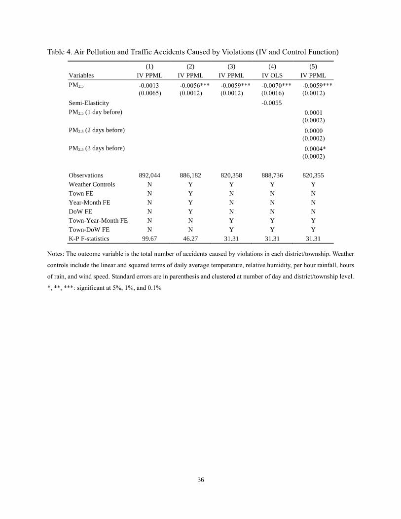
36

Table 4. Air Pollution and Traffic Accidents Caused by Violations (IV and Control Function)

(1) (2) (3) (4) (5)

Variables IV PPML IV PPML IV PPML IV OLS IV PPML

PM2.5 -0.0013 -0.0056*** -0.0059*** -0.0070*** -0.0059***

(0.0065) (0.0012) (0.0012) (0.0016) (0.0012)

Semi-Elasticity -0.0055

PM2.5 (1 day before) 0.0001

(0.0002)

PM2.5 (2 days before) 0.0000

(0.0002)

PM2.5 (3 days before) 0.0004*

(0.0002)

Observations 892,044 886,182 820,358 888,736 820,355

Weather Controls N Y Y Y Y

Town FE N Y N N N

Year-Month FE N Y N N N

DoW FE N Y N N N

Town-Year-Month FE N N Y Y Y

Town-DoW FE N N Y Y Y

K-P F-statistics 99.67 46.27 31.31 31.31 31.31

Notes: The outcome variable is the total number of accidents caused by violations in each district/township. Weather

controls include the linear and squared terms of daily average temperature, relative humidity, per hour rainfall, hours

of rain, and wind speed. Standard errors are in parenthesis and clustered at number of day and district/township level.

*, **, ***: significant at 5%, 1%, and 0.1%

37

Table 5. Robustness Checks: Heterogenous Effects across Traffic Patterns, Lagged Effects, and Effect on Errors

(1) (2) (3) (4) (5) (6) (7) (8) (9)

Variables Rush Hours Non-rush

Hours

Weekdays Weekend

At

Intersections

Not at

Intersections

Regions w/

Low Pop

Regions w/

High Pop

Mindless

Errors

PM2.5 -0.0068*** -0.0052*** -0.0060*** -0.0060** -0.0054*** -0.0070*** -0.0064* -0.0057*** -0.0032 (0.0017) (0.0013) (0.0014) (0.0023) (0.0013) (0.0018) (0.0032) (0.0013) (0.0019)

Observations 763,893 789,956 568,466 211,482 748,712 782,263 375,139 445,219 776,785

Notes: The outcome variable is the associated number of accidents in each district/township in model 1 to 8, and that caused by errors in model 9. All models

control for Town-Year-Month and Town-DoW fixed effects as well as weather controls including the linear and squared terms of daily average temperature, relative

humidity, per hour rainfall, hours of rain, and wind speed. PM2.5 concentration is instrumented by wind directions. Standard errors are in parenthesis and clustered

at number of day and district/township level.

*, **, ***: significant at 5%, 1%, and 0.1%

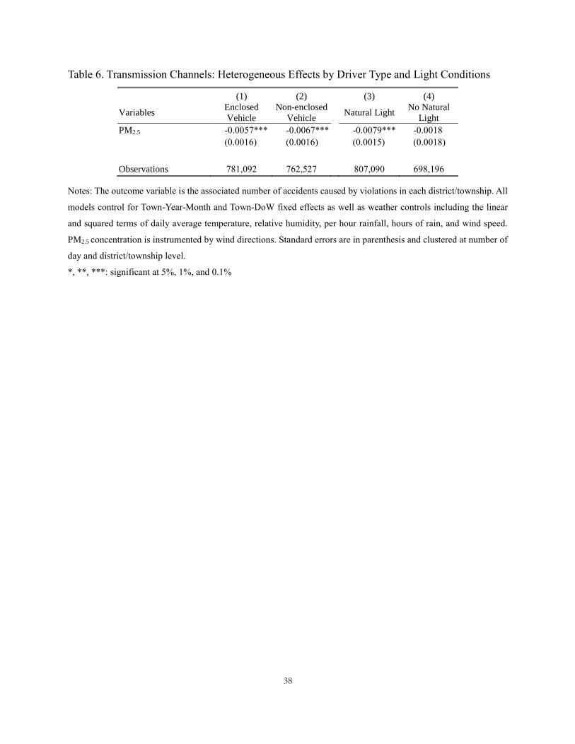
38

Table 6. Transmission Channels: Heterogeneous Effects by Driver Type and Light Conditions

(1) (2) (3) (4)

Variables Enclosed

Vehicle

Non-enclosed

Vehicle

Natural Light

No Natural

Light

PM2.5 -0.0057*** -0.0067*** -0.0079*** -0.0018 (0.0016) (0.0016) (0.0015) (0.0018)

Observations 781,092 762,527 807,090 698,196

Notes: The outcome variable is the associated number of accidents caused by violations in each district/township. All

models control for Town-Year-Month and Town-DoW fixed effects as well as weather controls including the linear

and squared terms of daily average temperature, relative humidity, per hour rainfall, hours of rain, and wind speed.

PM2.5 concentration is instrumented by wind directions. Standard errors are in parenthesis and clustered at number of

day and district/township level.

*, **, ***: significant at 5%, 1%, and 0.1%

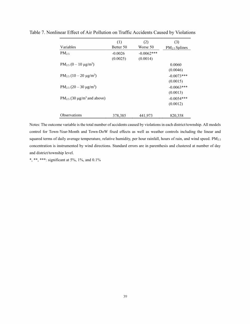
39

Table 7. Nonlinear Effect of Air Pollution on Traffic Accidents Caused by Violations

(1) (2) (3)

Variables Better 50 Worse 50 PM2.5 Splines

PM2.5 -0.0026 -0.0062*** (0.0025) (0.0014)

PM2.5 (0 – 10 μg/m3) 0.0060

(0.0046)

PM2.5 (10 – 20 μg/m3) -0.0073***

(0.0015)

PM2.5 (20 – 30 μg/m3) -0.0063***

(0.0013)

PM2.5 (30 μg/m3 and above) -0.0054***

(0.0012)

Observations 378,385 441,973 820,358

Notes: The outcome variable is the total number of accidents caused by violations in each district/township. All models

control for Town-Year-Month and Town-DoW fixed effects as well as weather controls including the linear and

squared terms of daily average temperature, relative humidity, per hour rainfall, hours of rain, and wind speed. PM2.5

concentration is instrumented by wind directions. Standard errors are in parenthesis and clustered at number of day

and district/township level.

*, **, ***: significant at 5%, 1%, and 0.1%

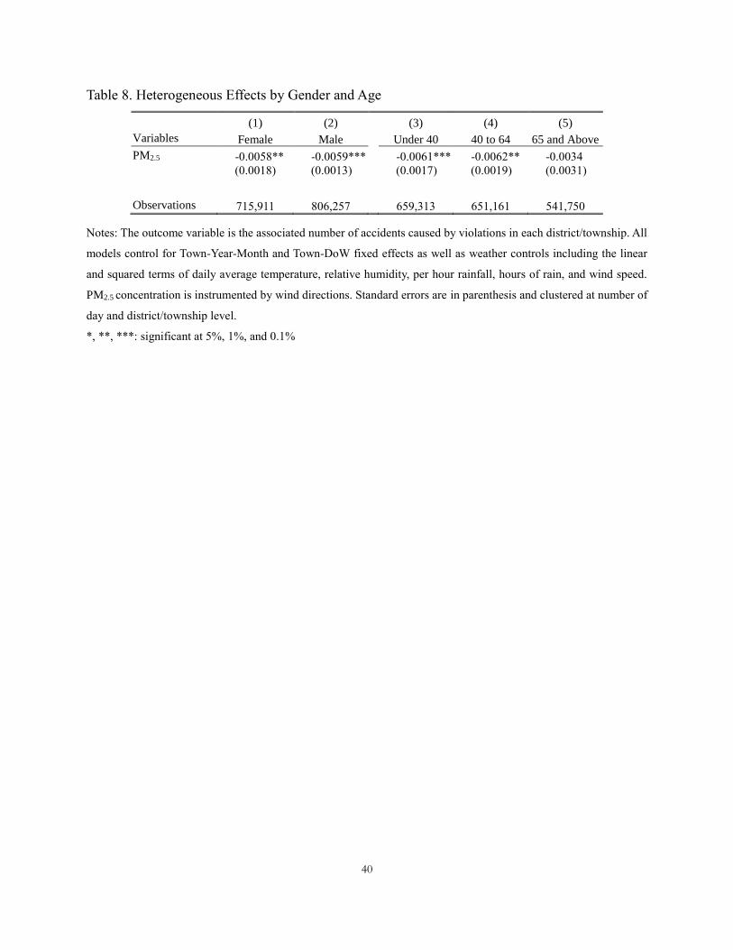
40

Table 8. Heterogeneous Effects by Gender and Age

(1) (2) (3) (4) (5)

Variables Female Male Under 40 40 to 64 65 and Above

PM2.5 -0.0058** -0.0059*** -0.0061*** -0.0062** -0.0034 (0.0018) (0.0013) (0.0017) (0.0019) (0.0031)

Observations 715,911 806,257 659,313 651,161 541,750

Notes: The outcome variable is the associated number of accidents caused by violations in each district/township. All

models control for Town-Year-Month and Town-DoW fixed effects as well as weather controls including the linear

and squared terms of daily average temperature, relative humidity, per hour rainfall, hours of rain, and wind speed.

PM2.5 concentration is instrumented by wind directions. Standard errors are in parenthesis and clustered at number of

day and district/township level.

*, **, ***: significant at 5%, 1%, and 0.1%

41

Figures

Figure 1. PM2.5 Concentration by District/Township in Taiwan, 2009 – 2015

Notes: The cutoffs are 20, 40, 60, 80 centiles, respectively.

PM2.5 concentration (ug/m3)

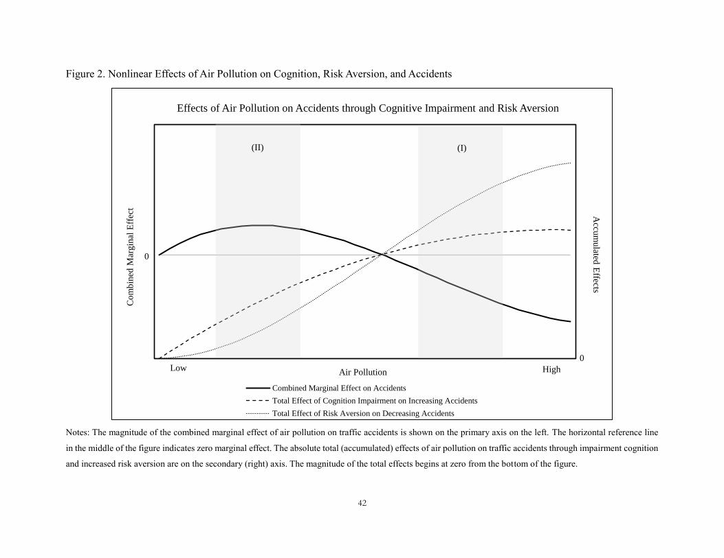
42

Figure 2. Nonlinear Effects of Air Pollution on Cognition, Risk Aversion, and Accidents

Notes: The magnitude of the combined marginal effect of air pollution on traffic accidents is shown on the primary axis on the left. The horizontal reference line

in the middle of the figure indicates zero marginal effect. The absolute total (accumulated) effects of air pollution on traffic accidents through impairment cognition

and increased risk aversion are on the secondary (right) axis. The magnitude of the total effects begins at zero from the bottom of the figure.

Air Pollution

Effects of Air Pollution on Accidents through Cognitive Impairment and Risk Aversion

Combined Marginal Effect on Accidents

Total Effect of Cognition Impairment on Increasing Accidents

Total Effect of Risk Aversion on Decreasing Accidents

HighLow

Co

mb

ined

Mar

gin

al E

ffec

t

0

Accu

mulated

Effects

0

(II) (I)

i

Appendix

Table A1. Air Pollution and Traffic Accidents Caused by Violations (Fixed Effects Models)

(1) (2) (3) (4) (5)

PPML PPML PPML PPML OLS

Variables Coefficient SE Coefficient SE Coefficient SE Coefficient SE Coefficient SE

PM2.5 0.0092*** (0.0016) 0.0120*** (0.0021) -0.0010*** (0.0002) -0.0009*** (0.0001) -0.0012*** (0.0002)

Temp. (°C) -0.1660*** (0.0178) -0.0068 (0.0042) -0.0097* (0.0046)

[Temp. (°C)]2 0.0044*** (0.0005) 0.0003** (0.0001) 0.0004** (0.0001)

Rainfall (mm/hr) -0.0325 (0.0372) -0.0212** (0.0070) -0.0195** (0.0069)

[Rainfall (mm/hr)]2 0.0009 (0.0024) -0.0015 (0.0009) -0.0016 (0.0009)

Rain hours (hr) 0.0008 (0.0073) -0.0023 (0.0013) -0.0016 (0.0013)

[Rain hours (hr)]2 -0.0000 (0.0002) -0.0001 (0.0001) -0.0001 (0.0001)

Relative Humidity (%) -0.0548** (0.0171) -0.0001 (0.0037) -0.0028 (0.0035)

[Relative Humidity (%)]2 0.0004*** (0.0001) -0.0000 (0.0000) -0.0000 (0.0000)

Wind Speed (m/s) 0.0868 (0.0964) 0.0493*** (0.0085) 0.0355*** (0.0073)

[Wind Speed (m/s)]2 -0.0220 (0.0117) -0.0061*** (0.0014) -0.0042*** (0.0013)

Constant -0.0247 (0.0844) 3.2903*** (0.7548) 1.0937*** (0.1533) 1.2706*** (0.1471) 1.8061*** (0.2171)

Observations 892,044 888,736 886,182 820,358 888,736

Weather Controls N Y Y Y Y

Town FE N N Y N N

Year-Month FE N N Y N N

DoW FE N N Y N N

Town-Year-Month FE N N N Y Y

Town-DoW FE N N N Y Y

Pseudo R2 / Adj-R2 0.00759 0.0147 0.468 0.465 0.734

Notes: This table presents complete results of table 2. The outcome variable is the total number of accidents caused by violations in each district/township. Standard

errors are clustered at number of day and district/township level.

*, **, ***: significant at 5%, 1%, and 0.1%

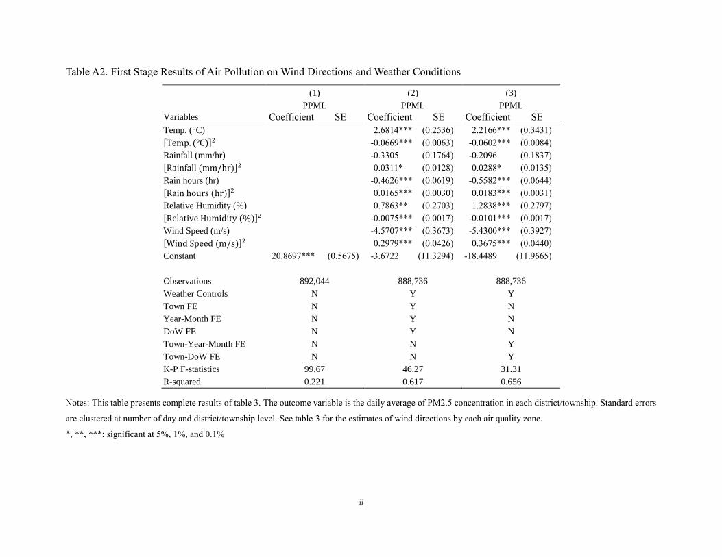
ii

Table A2. First Stage Results of Air Pollution on Wind Directions and Weather Conditions

(1) (2) (3)

PPML PPML PPML

Variables Coefficient SE Coefficient SE Coefficient SE

Temp. (°C) 2.6814*** (0.2536) 2.2166*** (0.3431)

[Temp. (°C)]2 -0.0669*** (0.0063) -0.0602*** (0.0084)

Rainfall (mm/hr) -0.3305 (0.1764) -0.2096 (0.1837)

[Rainfall (mm/hr)]2 0.0311* (0.0128) 0.0288* (0.0135)

Rain hours (hr) -0.4626*** (0.0619) -0.5582*** (0.0644)

[Rain hours (hr)]2 0.0165*** (0.0030) 0.0183*** (0.0031)

Relative Humidity (%) 0.7863** (0.2703) 1.2838*** (0.2797)

[Relative Humidity (%)]2 -0.0075*** (0.0017) -0.0101*** (0.0017)

Wind Speed (m/s) -4.5707*** (0.3673) -5.4300*** (0.3927)

[Wind Speed (m/s)]2 0.2979*** (0.0426) 0.3675*** (0.0440)

Constant 20.8697*** (0.5675) -3.6722 (11.3294) -18.4489 (11.9665)

Observations 892,044 888,736 888,736

Weather Controls N Y Y

Town FE N Y N

Year-Month FE N Y N

DoW FE N Y N

Town-Year-Month FE N N Y

Town-DoW FE N N Y

K-P F-statistics 99.67 46.27 31.31

R-squared 0.221 0.617 0.656

Notes: This table presents complete results of table 3. The outcome variable is the daily average of PM2.5 concentration in each district/township. Standard errors

are clustered at number of day and district/township level. See table 3 for the estimates of wind directions by each air quality zone.

*, **, ***: significant at 5%, 1%, and 0.1%

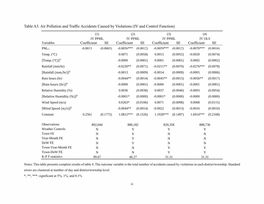
iii

Table A3. Air Pollution and Traffic Accidents Caused by Violations (IV and Control Function)

(1) (2) (3) (4)

IV PPML IV PPML IV PPML IV OLS

Variables Coefficient SE Coefficient SE Coefficient SE Coefficient SE

PM2.5 -0.0013 (0.0065) -0.0056*** (0.0012) -0.0059*** (0.0012) -0.0070*** (0.0016)

Temp. (°C) 0.0071 (0.0058) 0.0013 (0.0055) -0.0020 (0.0074)

[Temp. (°C)]2 -0.0000 (0.0001) 0.0001 (0.0001) 0.0002 (0.0002)

Rainfall (mm/hr) -0.0230** (0.0071) -0.0211** (0.0070) -0.0276*** (0.0078)

[Rainfall (mm/hr)]2 -0.0013 (0.0009) -0.0014 (0.0009) -0.0005 (0.0006)

Rain hours (hr) -0.0044** (0.0014) -0.0045** (0.0015) -0.0056** (0.0017)

[Rain hours (hr)]2 -0.0000 (0.0001) -0.0000 (0.0001) -0.0001 (0.0001)

Relative Humidity (%) 0.0036 (0.0038) 0.0037 (0.0040) -0.0003 (0.0054)

[Relative Humidity (%)]2 -0.0001* (0.0000) -0.0001* (0.0000) -0.0000 (0.0000)

Wind Speed (m/s) 0.0263* (0.0106) 0.0071 (0.0098) 0.0068 (0.0115)

[Wind Speed (m/s)]2 -0.0044** (0.0014) -0.0022 (0.0013) -0.0016 (0.0010)

Constant 0.2561 (0.1772) 1.0812*** (0.1526) 1.1928*** (0.1497) 1.6914*** (0.2168)

Observations 892,044 886,182 820,358 888,736

Weather Controls N Y Y Y

Town FE N Y N N

Year-Month FE N Y N N

DoW FE N Y N N

Town-Year-Month FE N N Y Y

Town-DoW FE N N Y Y

K-P F-statistics 99.67 46.27 31.31 31.31

Notes: This table presents complete results of table 4. The outcome variable is the total number of accidents caused by violations in each district/township. Standard

errors are clustered at number of day and district/township level.

*, **, ***: significant at 5%, 1%, and 0.1%

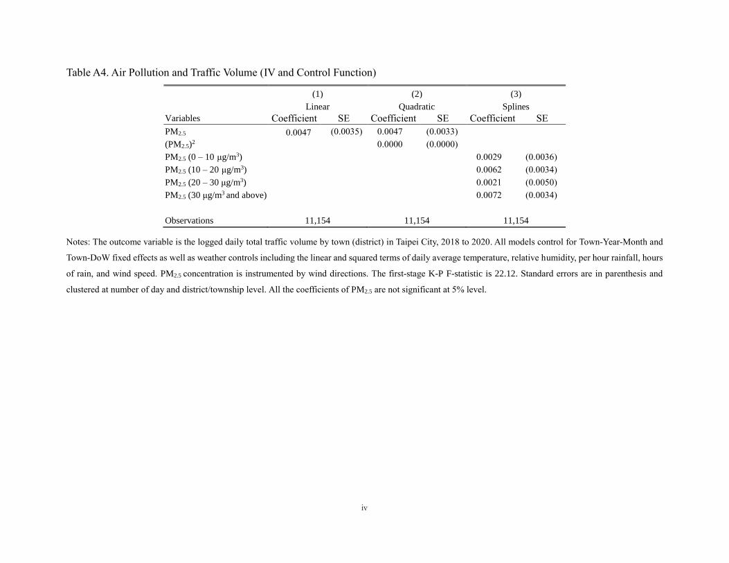
iv

Table A4. Air Pollution and Traffic Volume (IV and Control Function)

(1) (2) (3)

Linear Quadratic Splines

Variables Coefficient SE Coefficient SE Coefficient SE

PM2.5 0.0047 (0.0035) 0.0047 (0.0033)

(PM2.5)2 0.0000 (0.0000)

PM2.5 (0 – 10 μg/m3) 0.0029 (0.0036)

PM2.5 (10 – 20 μg/m3) 0.0062 (0.0034)

PM2.5 (20 – 30 μg/m3) 0.0021 (0.0050)

PM2.5 (30 μg/m3 and above) 0.0072 (0.0034)

Observations 11,154 11,154 11,154

Notes: The outcome variable is the logged daily total traffic volume by town (district) in Taipei City, 2018 to 2020. All models control for Town-Year-Month and

Town-DoW fixed effects as well as weather controls including the linear and squared terms of daily average temperature, relative humidity, per hour rainfall, hours

of rain, and wind speed. PM2.5 concentration is instrumented by wind directions. The first-stage K-P F-statistic is 22.12. Standard errors are in parenthesis and

clustered at number of day and district/township level. All the coefficients of PM2.5 are not significant at 5% level.

v

Table A5. Air Pollution and Traffic Accidents Caused by Violations (IV and Control Function)

(1) (2) (3) (4) (5)

Linear Weather Eight Wind Directions Four Wind Direction and

Wind Speed County Level

Sunny and Good

Visibility Only

Variables Coefficient SE Coefficient SE Coefficient SE Coefficient SE Coefficient SE

PM2.5 -0.0069*** (0.0011) -0.0055*** (0.0009) -0.0046*** (0.0006) -0.0069* (0.0029) -0.0061*** (0.0018)

Observations 820,358 820,358 820,358 48,518 804,604

Weather Controls

(Linear terms) Y Y Y Y Y

Weather Controls

(Quadratic terms) N Y Y Y Y

Town-Year-Month FE Y Y Y N Y

Town-DoW FE Y Y Y N Y

County-Year-Month FE N N N Y N

County-DoW FE N N N Y N

K-P F-statistics 34.02 19.27 55.39 23.95 31.31

Notes: The outcome variable is the total number of accidents caused by violations in each district/township. Model 1 includes only linear weather controls of daily

average temperature, relative humidity, per hour rainfall, hours of rain, and wind speed as well as Town-Year-Month and Town-DoW fixed effects. Model 2 uses

instrumental variables with eight wind directions and includes both linear and squared terms of weather controls. Model 3 uses wind speed and four wind directions

as the excluded instruments. Model 4 uses daily observations collapsed into county level. Model 5 uses the daily number of accidents caused by violations and

occurred in sunny days with good visibility at each district/township as the outcome variable. Standard errors in model 1, 2, 3, and 5, are clustered at number of

day and district/township level, while those in model 4 are clustered at number of day and county/level.

*, **, ***: significant at 5%, 1%, and 0.1%

vi

Table A6. Ozone and Traffic Accidents Caused by Violations (IV and Control Function)

(1) Ozone

Variables Coefficient SE

Ozone (ppm) 0.0003 (0.0008)

Observations 820,345

Weather Controls Y

Town-Year-Month FE Y

Town-DoW FE Y

K-P F-statistics 57.62

Notes: The outcome variable is the total number of accidents caused by violations in each district/township. The air pollutant variable is daily average of ozone

concentration (ppm) estimated by inverse distance weighting of the readings from three nearest air quality monitoring stations of each district/township. Weather

controls include the linear and squared terms of daily average temperature, relative humidity, per hour rainfall, hours of rain, and wind speed. Standard errors are

in parenthesis and clustered at number of day and district/township level.