Calving of a tidewater glacier driven by melting at the ... · Calving of a tidewater glacier driven by melting at ... We present a study of the development of a thermo-erosional

Calving of a tidewater glacier driven by melting at the waterline

Michał PĘTLICKI,1 Michał CIEPŁY,2 Jacek A. JANIA,2 Agnieszka PROMIŃSKA,3

Christophe KINNARD4

1Institute of Geophysics, Polish Academy of Sciences – Centre for Polar Studies KNOW (Leading National Research Centre),Warsaw, Poland

2Faculty of Earth Sciences, University of Silesia – Centre for Polar Studies KNOW (Leading National Research Centre),Sosnowiec, Poland

3Institute of Oceanology, Polish Academy of Sciences – Centre for Polar Studies KNOW (Leading National Research Centre),Sopot, Poland

4Département des Sciences de l’Environnement, Université du Québec à Trois-Rivières, Trois-Rivières, Québec, CanadaCorrespondence: Michał Pętlicki <[email protected]>

ABSTRACT. We present a study of the development of a thermo-erosional notch at the waterline and itsinfluence on calving of Hansbreen, a medium-sized grounded tidewater glacier in southern Svalbard.The study is based on the results of undercut notch melt modelling, based on measurements of sea-waterproperties, repeated terrestrial laser scans and analysis of time-lapse camera images. There is a strongcorrelation between observed calving activity and modelled melt rate of the undercut notch. Measureddepths of the undercut reach 4 m and vary greatly over time. The calving activity of Hansbreen wassignificantly lower in 2011 than in 2012, due to the persistent presence of the ice pack in Hornsund fjord,which cooled the sea surface and suppressed the wave action. Calving on Hansbreen is controlled by alocal imbalance of forces at the front, due to thermo-erosional undercutting at the sea waterline. Calvingactivity is therefore sensitive to changes in sea-water temperature and wave height. It may be expectedthat calving rates will rise with increased advection of warm oceanic water to the Arctic.

KEYWORDS: Arctic glaciology, calving, glacier calving, ice/ocean interactions

INTRODUCTIONThe largest component of ablation of the world’s cryosphereis calving (Van der Veen, 2002), i.e. the mechanical loss ofice from glaciers and ice shelves (Benn and others, 2007a). Ithas been shown that intense calving can lead to abruptchanges in glacial dynamics, enhancing ice flow by reducingthe back-stress (Joughin and others, 2004). The relationshipbetween observed calving rates and water depth followsregional clusters (Haresign, 2004), indicating the existence ofregional differences in the behaviour of calving fronts. Acomprehensive review of calving processes and theirmodelling is given by Benn and others (2007a). Theypropose a classification of calving mechanisms based ontheir relative importance. The first-order mechanism ofcalving is fracture propagation caused by longitudinalstresses driven by acceleration of the front. Fracture propa-gation can be enhanced by the presence of water increvasses (e.g. Weertman, 1973; Van der Veen, 1998; Alleyand others, 2005), either due to surface melt or rainfall.According to Benn and others (2007a) this mechanismusually controls the overall calving flux of tidewater glaciers.Another, generally less efficient calving mechanism, is

undercutting of the ice cliff by melting at or below thewaterline and the subsequent break-off of ice slabs. Bennand others (2007a) classify this as the second-order mech-anism. In this context, melt is less important as a mass sink,but is rather a source of force imbalance at the front and thusa trigger for calving (Vieli and others, 2001). Watertemperature and circulation control the melt (e.g. Eijpenand others, 2003; Motyka and others, 2003; Jenkins, 2011)and therefore this calving mechanism. Enhanced submarinemelt due to increased water circulation in the vicinity of

subglacial outflows is particularly strong, as buoyant freshwater draws in warm sea water (Motyka and others, 2013).As pointed out by Benn and others (2007a), second-ordercalving may play the major role for tidewater glaciers withlow longitudinal strain rates, i.e. where the velocitygradients are not high enough to cause intense fracturing.In such cases the undercutting of the calving front bymelting at or below the waterline and the resulting localimbalance of force at the front will cause calving events of asmaller size. The relative importance of this type of calvingremains unknown (Otero and others, 2010) and it is nottaken into account in models (Amundson and Truffer, 2010;Nick and others, 2010; Otero and others, 2010), as it wasprimarily investigated for the case of freshwater calving (e.g.Iken, 1977; Kirkbride and Warren, 1997; Haresign, 2004;Rohl, 2006).Vieli and others (2002) hypothesized that, for Hansbreen,

melt at the waterline is responsible for the mean summercalving rate, whereas major changes in the terminusposition are driven by bed topography. They assumed thatthe calving rate due to melt at the waterline throughout thesummer was constant and equal to the notch melting rate.Therefore, they accounted only for calving of the over-hanging slabs, while recent work of O’Leary and Christof-fersen (2013) shows that the undercut notch may influencethe stress field relatively deep into the glacier, causing thecalving rate to increase as much as three times, comparedwith a vertical ice cliff with no undercut.There are three main ways to quantitatively model the

calving rates: the first links the calving rate to an independentvariable, such as water depth or ice front height (e.g. Meierand Post, 1987; Pelto and Warren, 1991; Oerlemans and

Journal of Glaciology, Vol. 61, No. 229, 2015 doi: 10.3189/2015JoG15J062 851

others, 2011); the second specifies the terminus positionbased on the flotation criterion, which is the height abovebuoyancy at the glacier terminus (e.g. Brown and others,1982; Sikonia, 1982; Venteris, 1999; Vieli and others, 2002);the third, and most modern (e.g. Amundson and Truffer,2010; Nick and others, 2010; Otero and others, 2010),resolves the force balance at the front and applies it tocompute transverse crevasse depth (Nye, 1955, 1957), basedon the criterion proposed by Benn and others (2007b).Recent studies focus more on the detailed dynamics of

the front (e.g. O’Leary and Christoffersen, 2013) to accountfor more subtle effects, such as front geometry. Nonetheless,regardless of its importance for regional mass balance, andthus sea-level rise, calving and related dynamic processesare still poorly represented in state-of-the-art ice-sheetmodels (Benn and others, 2007a). One of the reasons forthis is the difficulty of collecting field data to quantifyprocesses, as long-term studies of calving rates are generallybased on remote-sensing methods whose time resolution islower than the processes involved (e.g. Blaszczyk andothers, 2009; Mansell and others, 2012). There is a lack ofdetailed observations at the scale of single events.Time-lapse photography is a widely used technique (e.g.

Kirkbride and Warren, 1997; O’Neel and others, 2003;Murray and others, 2015). It provides data at a relativelyhigh spatial resolution and usually at up to hourly samplingintervals. However, time-lapse photography is usuallyunable to produce precise quantitative results on its own(O’Neel and others, 2010), although recently it proved to bereliable for fast-flowing glaciers (Rivera and others, 2012). Amethod that has attracted much interest in recent years is‘structure-from-motion’ photogrammetry (Westoby andothers, 2012), mainly because of its ease of use and lowcost. In Ryan and others (2015) this method was applied toStore Glacier, Greenland, but, due to low temporal and

spatial resolution, it was possible to track only relativelylarge calving events. Another method, airborne laserscanning, is mainly used to provide a single digital terrainmodel that can be utilized as a reference surface for othersurveying methods (e.g. Murray and others, 2015). How-ever, repeated surveys that could capture single calvingevents are limited, due to the high cost of flights. Indirectmethods, such as seismic activity (O’Neel and others, 2010;Köhler and others, 2012), underwater acoustics (Pettit,2012; Glowacki and others, 2015) and floating iceberg size(Budd and others, 1980), need to be complemented withdirect methods to provide reliable quantitative data.The main objective of this study is to quantify the effect of

marine forcing on the calving processes of Hansbreen and,in particular, to verify the influence of thermo-erosionalundercutting on calving activity with field data.

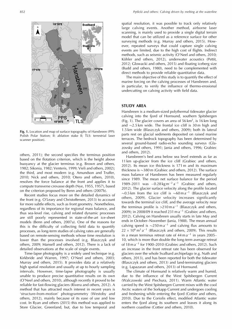
STUDY AREAHansbreen is a medium-sized polythermal tidewater glaciercalving into the fjord of Hornsund, southern Spitsbergen(Fig. 1). The glacier covers an area of 56 km2, is 16 km longand �2.5 km wide. The frontal ice cliff is 30m high and1.5 km wide (Blaszczyk and others, 2009); both its lateralparts rest on glacial sediments deposited on raised marineterraces. The bedrock topography has been determined byseveral ground-based radio-echo sounding surveys (Gla-zovsky and others, 1991; Jania and others, 1996; Grabiecand others, 2012).Hansbreen’s bed area below sea level extends as far as

11 km up-glacier from the ice cliff (Grabiec and others,2012). Its mean ice thickness is 171m and its maximumthickness is �380m (Grabiec and others, 2012). The surfacemass balance of Hansbreen has been measured regularlysince 1989. The mean net surface balance for the period1989–2011 was � 0:28 kgm� 2 a� 1 (Grabiec and others,2012). The glacier surface velocity along the profile located�0.5 km from the ice cliff is �60ma� 1 (Blaszczyk andothers, 2009). Glacier velocity increases significantlytowards the terminal ice cliff, and the average velocity nearthe terminus profile is >210ma� 1 (Blaszczyk and others,2009); in 2008/09 it reached 231ma� 1 (Grabiec and others,2012). Calving on Hansbreen usually starts in late May andends in October–November (Jania, 1988). The mean annualcalving speed is �250ma� 1 and calving flux amounts to22� 106 m3 a� 1 (Blaszczyk and others, 2009). This resultsin a mean terminus retreat rate of 44ma� 1 in years 2005–10, which is more than double the long-term average retreatof 18ma� 1 for 1900–2010 (Grabiec and others, 2012). Suchan increase in the front retreat rate has been observed forglaciers over the whole Svalbard archipelago (e.g. Nuth andothers, 2013), and has been reported for both the tidewater(Blaszczyk and others, 2013) and land-terminating glaciers(e.g. Lapazaran and others, 2013) of Hornsund.The climate of Hornsund is relatively warm and humid,

due to the influence of the West Spitsbergen Current(Walczowski and Piechura, 2011). Warm Atlantic watercarried by the West Spitsbergen Current mixes with the coolArctic waters of the Sorkapp Current and undergoes coolingand freshening while entering the fjord (Cottier and others,2010). Due to the Coriolis effect, modified Atlantic waterenters the fjord along its southern and leaves it along itsnorthern coastline (Cottier and others, 2010).

Fig. 1. Location and map of surface topography of Hansbreen (PPS:Polish Polar Station; II: ablation stake II; TLS: terrestrial laserscanner position).

Pętlicki and others: Calving driven by melting at the waterline852

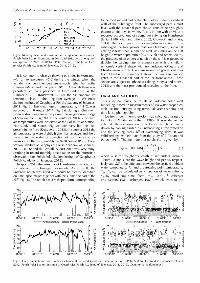
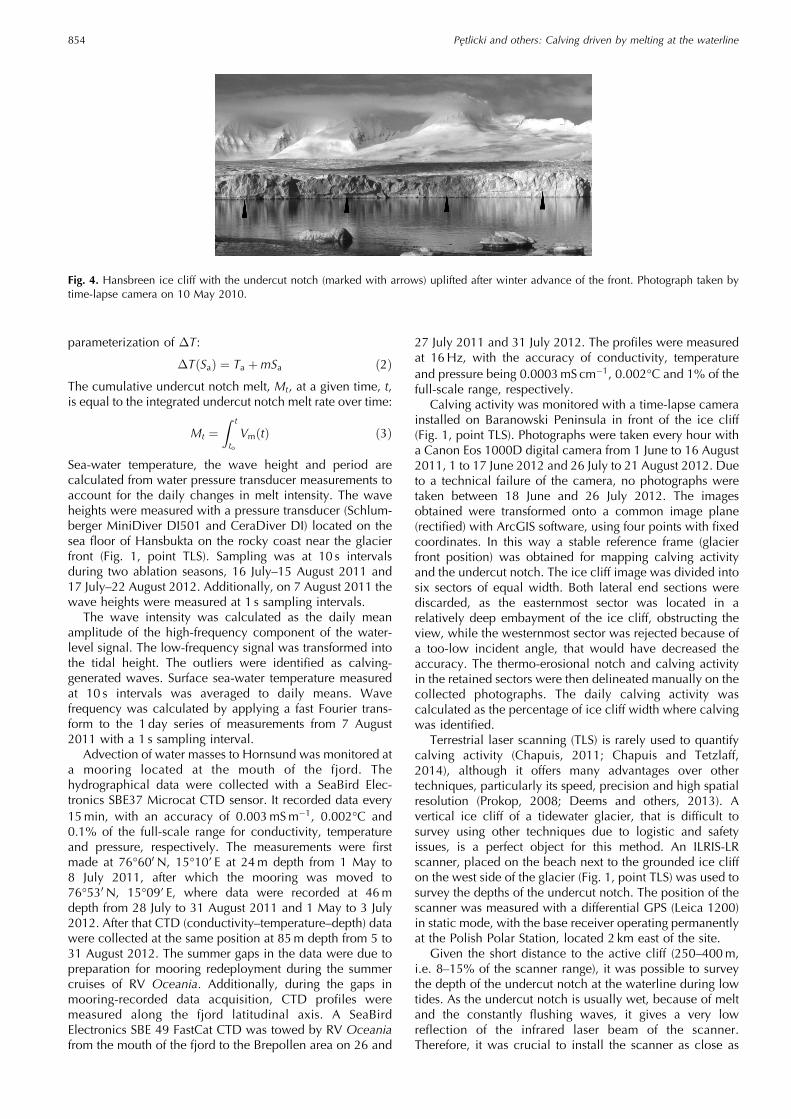
It is common to observe thawing episodes in Hornsund,with air temperatures >0°C during the winter, when thevariability of the air temperature is much higher than in thesummer (Marsz and Styszyńska, 2013). Although there waspersistent ice pack presence in Hornsund fjord in thesummer of 2011 (Kruszewski, 2012), the air temperaturesremained close to the long-term average (Polish PolarStation, Institute of Geophysics Polish Academy of Sciences,2011; Fig. 2). The maximum air temperature, 11.1°C, wasrecorded on 18 August 2011 (Fig. 3a), during a föhn eventwhen a strong eastern wind passed the neighbouring ridgeof Sofiekammen (Fig. 3b). In the winter of 2011/12 positiveair temperatures were observed at the Polish Polar Station,Hornsund, until March (Fig. 2), with very little sea icepresent in the fjord (Kruszewski, 2013). In summer 2012 theair temperatures were slightly higher than average, and therewere a few episodes of advection of warm oceanic airmasses from the west, notably on 8–18 August (Polish PolarStation, Institute of Geophysics Polish Academy of Sciences,2012; Fig. 3c and d). Overall, August 2012 was very rainy,resulting in record monthly precipitation for the Hornsundobservation site (Polish Polar Station, Institute of GeophysicsPolish Academy of Sciences, 2012).In spring 2010 the terminus of Hansbreen advanced and

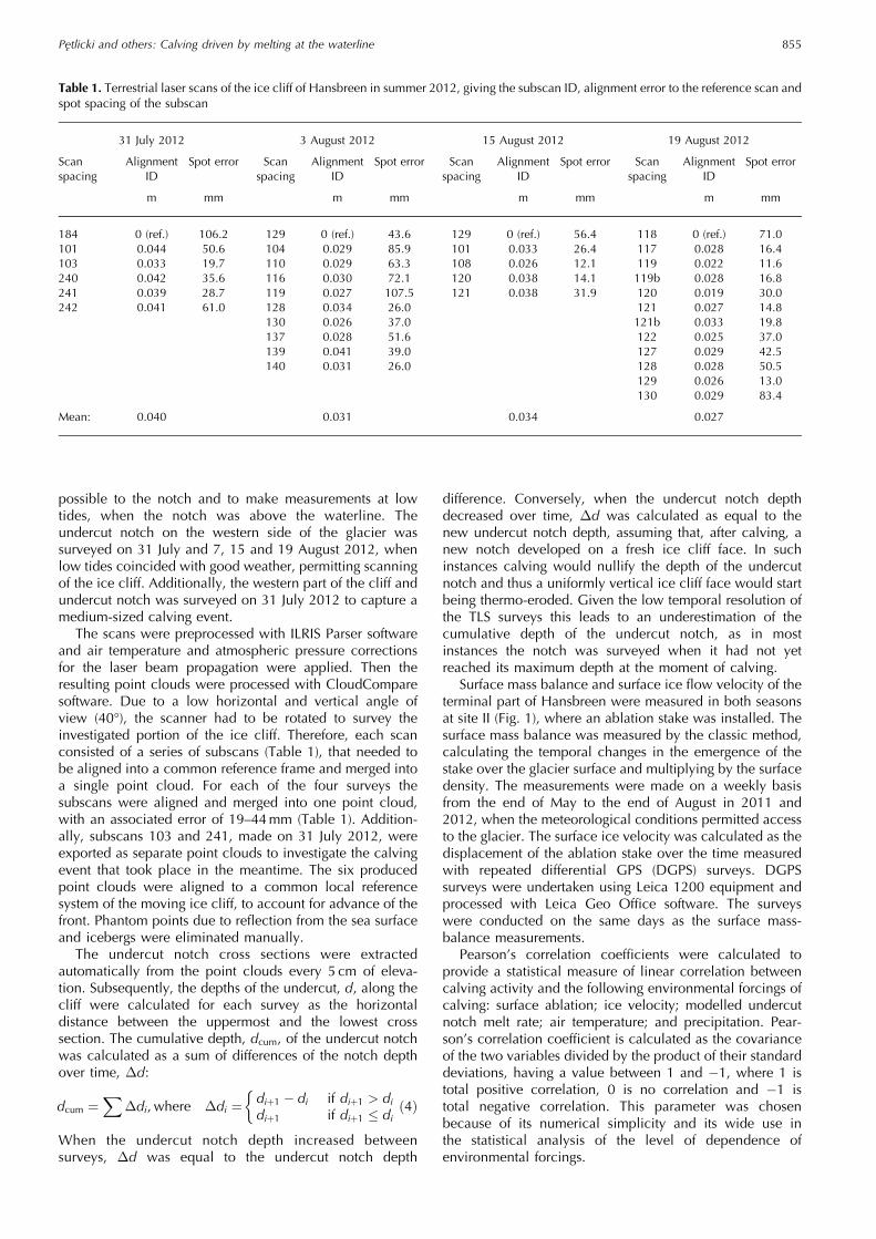
slid above the submerged sediments. As a result, theundercut notch was lifted and could be clearly identifiedon time-lapse images together with the submarine part of thecliff (Fig. 4). The notch has a v-shaped form, corresponding

to the most incised part of the cliff. Below, there is a verticalwall of the submerged front. The submerged part, almostlevel with the subaerial part, shows signs of being slightlythermo-eroded by sea water. This is in line with previouslyreported observations of submarine calving on Hansbreen(Jania, 1988; Vieli and others, 2002; Glowacki and others,2015). The occurrence of buoyancy-driven calving of thesubmerged ice foot proves that, on Hansbreen, subaerialcalving is faster than submarine melt. Assuming an ice cliffheight to water depth ratio of 0.75 (Vieli and others, 2002),the presence of an undercut notch on the cliff is expected todouble the calving rate in comparison with a similarlyuniformly vertical shape with no undercut (O’Leary andChristoffersen, 2013). There are several subglacial outflowsfrom Hansbreen, manifested above the waterline as icegates in the subaerial part of the ice front above. Thesesectors are subject to enhanced calving (Motyka and others,2013) and the most pronounced recession of the front.

DATA AND METHODSThis study combines the results of undercut notch meltmodelling (based on measurements of sea-water properties)with ice front surveys using terrestrial laser scanning andtime-lapse photography.Ice front notch thermo-erosion was calculated using the

formula of White and others (1980). It was derived tocalculate the deterioration of icebergs, which is mainlydriven by calving caused by undercutting at the waterlineand the ensuing break off of overhanging slabs. It wasvalidated against field data from the study of El-Tahan andothers (1987). The melt rate of a notch, Vm, is given by:

Vm ¼ 0:000146Rh

� �0:2 h�

� �

�T ð1Þ

where R is the roughness length of ice surface (usually10mm), h and � are the wave height and period, respect-ively, and �T is the difference between the far-field ambientwater temperature, Ta, and the freezing point temperature,Tfp. Tfp can be calculated as a function of water salinity,Sa, by introducing a melt factor, m ¼ � 0:6�C � 1 (Josbergerand Martin, 1981; Josberger, 1983), which leads to the

Fig. 3. Daily precipitation sums, mean air temperature, wind speed and direction at Polish Polar Station Hornsund in summer 2011 and2012 (Polish Polar Station, Institute of Geophysics Polish Academy of Sciences, 2011, 2012). (Date format is dd/mm/yy.)

Fig. 2. Monthly mean and maximum air temperature measured atPolish Polar Station Hornsund in 2011 and 2012, and a long-termaverage for 1979–2010 (Polish Polar Station, Institute of Geo-physics Polish Academy of Sciences, 2011, 2012).

Pętlicki and others: Calving driven by melting at the waterline 853

parameterization of �T:

�T Sað Þ ¼ Ta þmSa ð2Þ

The cumulative undercut notch melt, Mt, at a given time, t,is equal to the integrated undercut notch melt rate over time:

Mt ¼

Z t

toVmðtÞ ð3Þ

Sea-water temperature, the wave height and period arecalculated from water pressure transducer measurements toaccount for the daily changes in melt intensity. The waveheights were measured with a pressure transducer (Schlum-berger MiniDiver DI501 and CeraDiver DI) located on thesea floor of Hansbukta on the rocky coast near the glacierfront (Fig. 1, point TLS). Sampling was at 10 s intervalsduring two ablation seasons, 16 July–15 August 2011 and17 July–22 August 2012. Additionally, on 7 August 2011 thewave heights were measured at 1 s sampling intervals.The wave intensity was calculated as the daily mean

amplitude of the high-frequency component of the water-level signal. The low-frequency signal was transformed intothe tidal height. The outliers were identified as calving-generated waves. Surface sea-water temperature measuredat 10 s intervals was averaged to daily means. Wavefrequency was calculated by applying a fast Fourier trans-form to the 1 day series of measurements from 7 August2011 with a 1 s sampling interval.Advection of water masses to Hornsund was monitored at

a mooring located at the mouth of the fjord. Thehydrographical data were collected with a SeaBird Elec-tronics SBE37 Microcat CTD sensor. It recorded data every15min, with an accuracy of 0.003mSm� 1, 0.002°C and0.1% of the full-scale range for conductivity, temperatureand pressure, respectively. The measurements were firstmade at 76°600N, 15°10’ E at 24m depth from 1 May to8 July 2011, after which the mooring was moved to76°530N, 15°09’ E, where data were recorded at 46mdepth from 28 July to 31 August 2011 and 1 May to 3 July2012. After that CTD (conductivity–temperature–depth) datawere collected at the same position at 85m depth from 5 to31 August 2012. The summer gaps in the data were due topreparation for mooring redeployment during the summercruises of RV Oceania. Additionally, during the gaps inmooring-recorded data acquisition, CTD profiles weremeasured along the fjord latitudinal axis. A SeaBirdElectronics SBE 49 FastCat CTD was towed by RV Oceaniafrom the mouth of the fjord to the Brepollen area on 26 and

27 July 2011 and 31 July 2012. The profiles were measuredat 16Hz, with the accuracy of conductivity, temperatureand pressure being 0.0003mS cm� 1, 0.002°C and 1% of thefull-scale range, respectively.Calving activity was monitored with a time-lapse camera

installed on Baranowski Peninsula in front of the ice cliff(Fig. 1, point TLS). Photographs were taken every hour witha Canon Eos 1000D digital camera from 1 June to 16 August2011, 1 to 17 June 2012 and 26 July to 21 August 2012. Dueto a technical failure of the camera, no photographs weretaken between 18 June and 26 July 2012. The imagesobtained were transformed onto a common image plane(rectified) with ArcGIS software, using four points with fixedcoordinates. In this way a stable reference frame (glacierfront position) was obtained for mapping calving activityand the undercut notch. The ice cliff image was divided intosix sectors of equal width. Both lateral end sections werediscarded, as the easternmost sector was located in arelatively deep embayment of the ice cliff, obstructing theview, while the westernmost sector was rejected because ofa too-low incident angle, that would have decreased theaccuracy. The thermo-erosional notch and calving activityin the retained sectors were then delineated manually on thecollected photographs. The daily calving activity wascalculated as the percentage of ice cliff width where calvingwas identified.Terrestrial laser scanning (TLS) is rarely used to quantify

calving activity (Chapuis, 2011; Chapuis and Tetzlaff,2014), although it offers many advantages over othertechniques, particularly its speed, precision and high spatialresolution (Prokop, 2008; Deems and others, 2013). Avertical ice cliff of a tidewater glacier, that is difficult tosurvey using other techniques due to logistic and safetyissues, is a perfect object for this method. An ILRIS-LRscanner, placed on the beach next to the grounded ice cliffon the west side of the glacier (Fig. 1, point TLS) was used tosurvey the depths of the undercut notch. The position of thescanner was measured with a differential GPS (Leica 1200)in static mode, with the base receiver operating permanentlyat the Polish Polar Station, located 2 km east of the site.Given the short distance to the active cliff (250–400m,

i.e. 8–15% of the scanner range), it was possible to surveythe depth of the undercut notch at the waterline during lowtides. As the undercut notch is usually wet, because of meltand the constantly flushing waves, it gives a very lowreflection of the infrared laser beam of the scanner.Therefore, it was crucial to install the scanner as close as

Fig. 4. Hansbreen ice cliff with the undercut notch (marked with arrows) uplifted after winter advance of the front. Photograph taken bytime-lapse camera on 10 May 2010.


possible to the notch and to make measurements at lowtides, when the notch was above the waterline. Theundercut notch on the western side of the glacier wassurveyed on 31 July and 7, 15 and 19 August 2012, whenlow tides coincided with good weather, permitting scanningof the ice cliff. Additionally, the western part of the cliff andundercut notch was surveyed on 31 July 2012 to capture amedium-sized calving event.The scans were preprocessed with ILRIS Parser software

and air temperature and atmospheric pressure correctionsfor the laser beam propagation were applied. Then theresulting point clouds were processed with CloudComparesoftware. Due to a low horizontal and vertical angle ofview (40°), the scanner had to be rotated to survey theinvestigated portion of the ice cliff. Therefore, each scanconsisted of a series of subscans (Table 1), that needed tobe aligned into a common reference frame and merged intoa single point cloud. For each of the four surveys thesubscans were aligned and merged into one point cloud,with an associated error of 19–44mm (Table 1). Addition-ally, subscans 103 and 241, made on 31 July 2012, wereexported as separate point clouds to investigate the calvingevent that took place in the meantime. The six producedpoint clouds were aligned to a common local referencesystem of the moving ice cliff, to account for advance of thefront. Phantom points due to reflection from the sea surfaceand icebergs were eliminated manually.The undercut notch cross sections were extracted

automatically from the point clouds every 5 cm of eleva-tion. Subsequently, the depths of the undercut, d, along thecliff were calculated for each survey as the horizontaldistance between the uppermost and the lowest crosssection. The cumulative depth, dcum, of the undercut notchwas calculated as a sum of differences of the notch depthover time, �d:

dcum ¼X

�di, where �di ¼diþ1 � di if diþ1 > didiþ1 if diþ1 � di

�

ð4Þ

When the undercut notch depth increased betweensurveys, �d was equal to the undercut notch depth

difference. Conversely, when the undercut notch depthdecreased over time, �d was calculated as equal to thenew undercut notch depth, assuming that, after calving, anew notch developed on a fresh ice cliff face. In suchinstances calving would nullify the depth of the undercutnotch and thus a uniformly vertical ice cliff face would startbeing thermo-eroded. Given the low temporal resolution ofthe TLS surveys this leads to an underestimation of thecumulative depth of the undercut notch, as in mostinstances the notch was surveyed when it had not yetreached its maximum depth at the moment of calving.Surface mass balance and surface ice flow velocity of the

terminal part of Hansbreen were measured in both seasonsat site II (Fig. 1), where an ablation stake was installed. Thesurface mass balance was measured by the classic method,calculating the temporal changes in the emergence of thestake over the glacier surface and multiplying by the surfacedensity. The measurements were made on a weekly basisfrom the end of May to the end of August in 2011 and2012, when the meteorological conditions permitted accessto the glacier. The surface ice velocity was calculated as thedisplacement of the ablation stake over the time measuredwith repeated differential GPS (DGPS) surveys. DGPSsurveys were undertaken using Leica 1200 equipment andprocessed with Leica Geo Office software. The surveyswere conducted on the same days as the surface mass-balance measurements.Pearson’s correlation coefficients were calculated to

provide a statistical measure of linear correlation betweencalving activity and the following environmental forcings ofcalving: surface ablation; ice velocity; modelled undercutnotch melt rate; air temperature; and precipitation. Pear-son’s correlation coefficient is calculated as the covarianceof the two variables divided by the product of their standarddeviations, having a value between 1 and � 1, where 1 istotal positive correlation, 0 is no correlation and � 1 istotal negative correlation. This parameter was chosenbecause of its numerical simplicity and its wide use inthe statistical analysis of the level of dependence ofenvironmental forcings.

Table 1. Terrestrial laser scans of the ice cliff of Hansbreen in summer 2012, giving the subscan ID, alignment error to the reference scan andspot spacing of the subscan

31 July 2012 3 August 2012 15 August 2012 19 August 2012

Scanspacing

AlignmentID

Spot error Scanspacing

AlignmentID


AlignmentID


AlignmentID

Spot error

m mm m mm m mm m mm

184 0 (ref.) 106.2 129 0 (ref.) 43.6 129 0 (ref.) 56.4 118 0 (ref.) 71.0101 0.044 50.6 104 0.029 85.9 101 0.033 26.4 117 0.028 16.4103 0.033 19.7 110 0.029 63.3 108 0.026 12.1 119 0.022 11.6240 0.042 35.6 116 0.030 72.1 120 0.038 14.1 119b 0.028 16.8241 0.039 28.7 119 0.027 107.5 121 0.038 31.9 120 0.019 30.0242 0.041 61.0 128 0.034 26.0 121 0.027 14.8

130 0.026 37.0 121b 0.033 19.8137 0.028 51.6 122 0.025 37.0139 0.041 39.0 127 0.029 42.5140 0.031 26.0 128 0.028 50.5

129 0.026 13.0130 0.029 83.4

Mean: 0.040 0.031 0.034 0.027


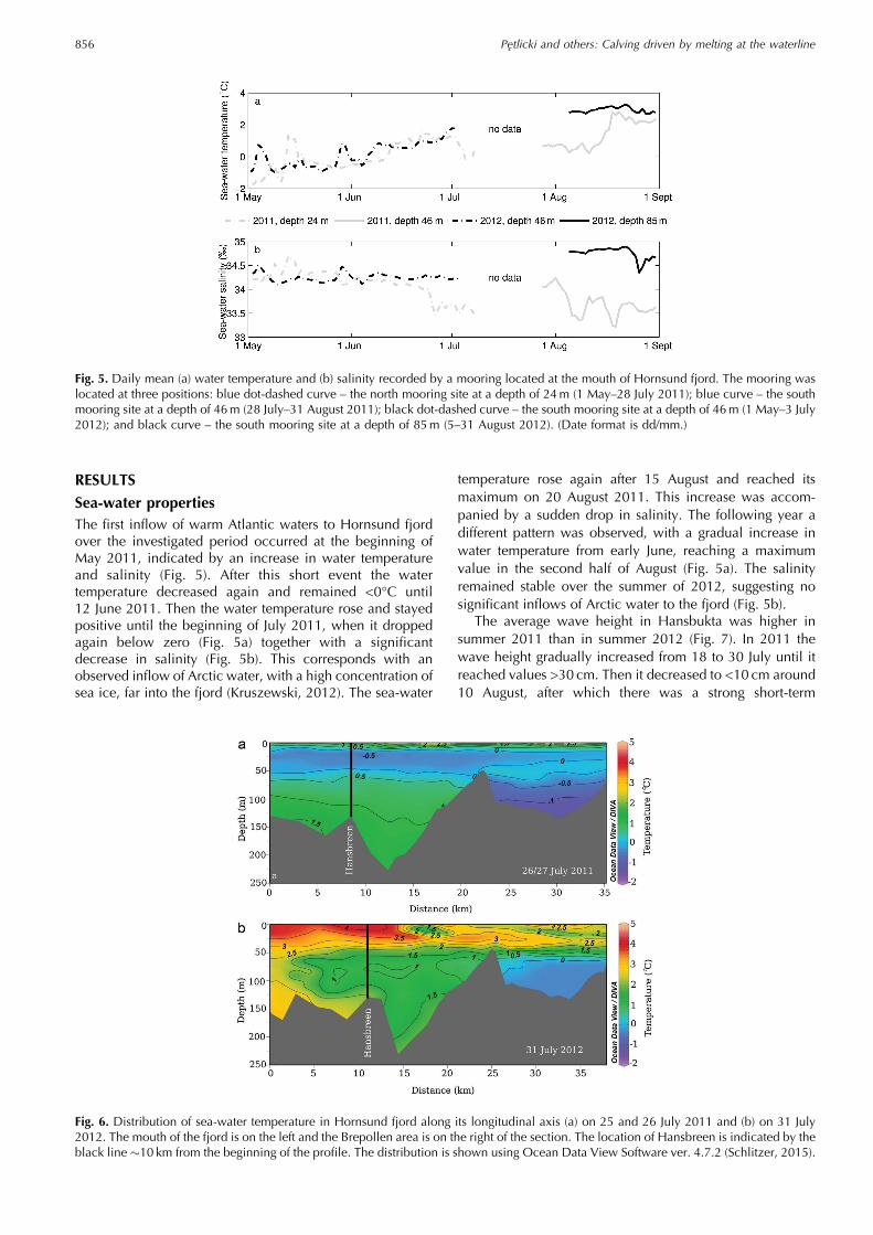
RESULTSSea-water propertiesThe first inflow of warm Atlantic waters to Hornsund fjordover the investigated period occurred at the beginning ofMay 2011, indicated by an increase in water temperatureand salinity (Fig. 5). After this short event the watertemperature decreased again and remained <0°C until12 June 2011. Then the water temperature rose and stayedpositive until the beginning of July 2011, when it droppedagain below zero (Fig. 5a) together with a significantdecrease in salinity (Fig. 5b). This corresponds with anobserved inflow of Arctic water, with a high concentration ofsea ice, far into the fjord (Kruszewski, 2012). The sea-water

temperature rose again after 15 August and reached itsmaximum on 20 August 2011. This increase was accom-panied by a sudden drop in salinity. The following year adifferent pattern was observed, with a gradual increase inwater temperature from early June, reaching a maximumvalue in the second half of August (Fig. 5a). The salinityremained stable over the summer of 2012, suggesting nosignificant inflows of Arctic water to the fjord (Fig. 5b).The average wave height in Hansbukta was higher in

summer 2011 than in summer 2012 (Fig. 7). In 2011 thewave height gradually increased from 18 to 30 July until itreached values >30 cm. Then it decreased to <10 cm around10 August, after which there was a strong short-term

Fig. 6. Distribution of sea-water temperature in Hornsund fjord along its longitudinal axis (a) on 25 and 26 July 2011 and (b) on 31 July2012. The mouth of the fjord is on the left and the Brepollen area is on the right of the section. The location of Hansbreen is indicated by theblack line �10 km from the beginning of the profile. The distribution is shown using Ocean Data View Software ver. 4.7.2 (Schlitzer, 2015).

Fig. 5. Daily mean (a) water temperature and (b) salinity recorded by a mooring located at the mouth of Hornsund fjord. The mooring waslocated at three positions: blue dot-dashed curve – the north mooring site at a depth of 24m (1 May–28 July 2011); blue curve – the southmooring site at a depth of 46m (28 July–31 August 2011); black dot-dashed curve – the south mooring site at a depth of 46m (1 May–3 July2012); and black curve – the south mooring site at a depth of 85m (5–31 August 2012). (Date format is dd/mm.)


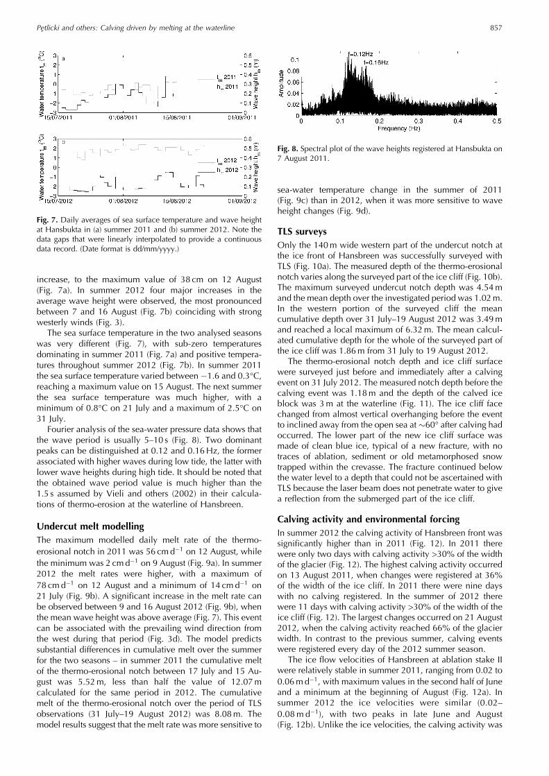
increase, to the maximum value of 38 cm on 12 August(Fig. 7a). In summer 2012 four major increases in theaverage wave height were observed, the most pronouncedbetween 7 and 16 August (Fig. 7b) coinciding with strongwesterly winds (Fig. 3).The sea surface temperature in the two analysed seasons

was very different (Fig. 7), with sub-zero temperaturesdominating in summer 2011 (Fig. 7a) and positive tempera-tures throughout summer 2012 (Fig. 7b). In summer 2011the sea surface temperature varied between � 1:6 and 0.3°C,reaching a maximum value on 15 August. The next summerthe sea surface temperature was much higher, with aminimum of 0.8°C on 21 July and a maximum of 2.5°C on31 July.Fourier analysis of the sea-water pressure data shows that

the wave period is usually 5–10 s (Fig. 8). Two dominantpeaks can be distinguished at 0.12 and 0.16Hz, the formerassociated with higher waves during low tide, the latter withlower wave heights during high tide. It should be noted thatthe obtained wave period value is much higher than the1.5 s assumed by Vieli and others (2002) in their calcula-tions of thermo-erosion at the waterline of Hansbreen.

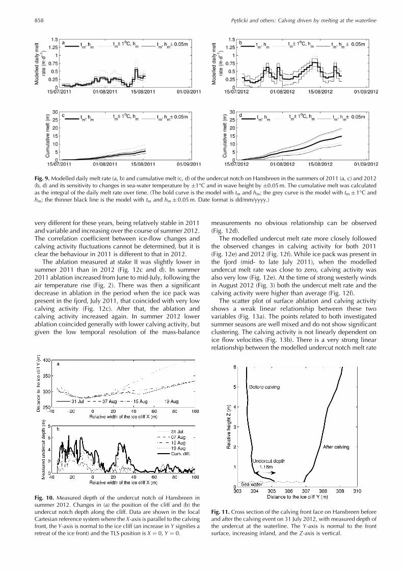
Undercut melt modellingThe maximum modelled daily melt rate of the thermo-erosional notch in 2011 was 56 cmd� 1 on 12 August, whilethe minimum was 2 cmd� 1 on 9 August (Fig. 9a). In summer2012 the melt rates were higher, with a maximum of78 cmd� 1 on 12 August and a minimum of 14 cmd� 1 on21 July (Fig. 9b). A significant increase in the melt rate canbe observed between 9 and 16 August 2012 (Fig. 9b), whenthe mean wave height was above average (Fig. 7). This eventcan be associated with the prevailing wind direction fromthe west during that period (Fig. 3d). The model predictssubstantial differences in cumulative melt over the summerfor the two seasons – in summer 2011 the cumulative meltof the thermo-erosional notch between 17 July and 15 Au-gust was 5.52m, less than half the value of 12.07mcalculated for the same period in 2012. The cumulativemelt of the thermo-erosional notch over the period of TLSobservations (31 July–19 August 2012) was 8.08m. Themodel results suggest that the melt rate was more sensitive to

sea-water temperature change in the summer of 2011(Fig. 9c) than in 2012, when it was more sensitive to waveheight changes (Fig. 9d).

TLS surveysOnly the 140m wide western part of the undercut notch atthe ice front of Hansbreen was successfully surveyed withTLS (Fig. 10a). The measured depth of the thermo-erosionalnotch varies along the surveyed part of the ice cliff (Fig. 10b).The maximum surveyed undercut notch depth was 4.54mand the mean depth over the investigated period was 1.02m.In the western portion of the surveyed cliff the meancumulative depth over 31 July–19 August 2012 was 3.49mand reached a local maximum of 6.32m. The mean calcul-ated cumulative depth for the whole of the surveyed part ofthe ice cliff was 1.86m from 31 July to 19 August 2012.The thermo-erosional notch depth and ice cliff surface

were surveyed just before and immediately after a calvingevent on 31 July 2012. The measured notch depth before thecalving event was 1.18m and the depth of the calved iceblock was 3m at the waterline (Fig. 11). The ice cliff facechanged from almost vertical overhanging before the eventto inclined away from the open sea at �60° after calving hadoccurred. The lower part of the new ice cliff surface wasmade of clean blue ice, typical of a new fracture, with notraces of ablation, sediment or old metamorphosed snowtrapped within the crevasse. The fracture continued belowthe water level to a depth that could not be ascertained withTLS because the laser beam does not penetrate water to givea reflection from the submerged part of the ice cliff.

Calving activity and environmental forcingIn summer 2012 the calving activity of Hansbreen front wassignificantly higher than in 2011 (Fig. 12). In 2011 therewere only two days with calving activity >30% of the widthof the glacier (Fig. 12). The highest calving activity occurredon 13 August 2011, when changes were registered at 36%of the width of the ice cliff. In 2011 there were nine dayswith no calving registered. In the summer of 2012 therewere 11 days with calving activity >30% of the width of theice cliff (Fig. 12). The largest changes occurred on 21 August2012, when the calving activity reached 66% of the glacierwidth. In contrast to the previous summer, calving eventswere registered every day of the 2012 summer season.The ice flow velocities of Hansbreen at ablation stake II

were relatively stable in summer 2011, ranging from 0.02 to0.06md� 1, with maximum values in the second half of Juneand a minimum at the beginning of August (Fig. 12a). Insummer 2012 the ice velocities were similar (0.02–0.08m d� 1), with two peaks in late June and August(Fig. 12b). Unlike the ice velocities, the calving activity was

Fig. 8. Spectral plot of the wave heights registered at Hansbukta on7 August 2011.

Fig. 7. Daily averages of sea surface temperature and wave heightat Hansbukta in (a) summer 2011 and (b) summer 2012. Note thedata gaps that were linearly interpolated to provide a continuousdata record. (Date format is dd/mm/yyyy.)


very different for these years, being relatively stable in 2011and variable and increasing over the course of summer 2012.The correlation coefficient between ice-flow changes andcalving activity fluctuations cannot be determined, but it isclear the behaviour in 2011 is different to that in 2012.The ablation measured at stake II was slightly lower in

summer 2011 than in 2012 (Fig. 12c and d). In summer2011 ablation increased from June to mid-July, following theair temperature rise (Fig. 2). There was then a significantdecrease in ablation in the period when the ice pack waspresent in the fjord, July 2011, that coincided with very lowcalving activity (Fig. 12c). After that, the ablation andcalving activity increased again. In summer 2012 lowerablation coincided generally with lower calving activity, butgiven the low temporal resolution of the mass-balance

measurements no obvious relationship can be observed(Fig. 12d).The modelled undercut melt rate more closely followed

the observed changes in calving activity for both 2011(Fig. 12e) and 2012 (Fig. 12f). While ice pack was present inthe fjord (mid- to late July 2011), when the modelledundercut melt rate was close to zero, calving activity wasalso very low (Fig. 12e). At the time of strong westerly windsin August 2012 (Fig. 3) both the undercut melt rate and thecalving activity were higher than average (Fig. 12f).The scatter plot of surface ablation and calving activity

shows a weak linear relationship between these twovariables (Fig. 13a). The points related to both investigatedsummer seasons are well mixed and do not show significantclustering. The calving activity is not linearly dependent onice flow velocities (Fig. 13b). There is a very strong linearrelationship between the modelled undercut notch melt rate

Fig. 11. Cross section of the calving front face on Hansbreen beforeand after the calving event on 31 July 2012, with measured depth ofthe undercut at the waterline. The Y-axis is normal to the frontsurface, increasing inland, and the Z-axis is vertical.

Fig. 9.Modelled daily melt rate (a, b) and cumulative melt (c, d) of the undercut notch on Hansbreen in the summers of 2011 (a, c) and 2012(b, d) and its sensitivity to changes in sea-water temperature by �1°C and in wave height by �0.05m. The cumulative melt was calculatedas the integral of the daily melt rate over time. (The bold curve is the model with tm and hm; the grey curve is the model with tm� 1°C andhm; the thinner black line is the model with tm and hm� 0.05m. Date format is dd/mm/yyyy.)

Fig. 10. Measured depth of the undercut notch of Hansbreen insummer 2012. Changes in (a) the position of the cliff and (b) theundercut notch depth along the cliff. Data are shown in the localCartesian reference system where the X-axis is parallel to the calvingfront, the Y-axis is normal to the ice cliff (an increase in Y signifies aretreat of the ice front) and the TLS position is X ¼ 0, Y ¼ 0.


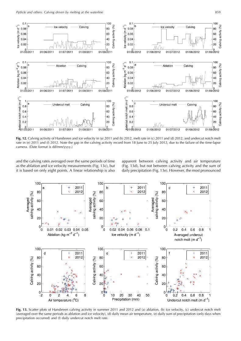
and the calving rates averaged over the same periods of timeas the ablation and ice velocity measurements (Fig. 13c), butit is based on only eight points. A linear relationship is also

apparent between calving activity and air temperature(Fig. 13d), but not between calving activity and the sum ofdaily precipitation (Fig. 13e). However, themost pronounced

Fig. 13. Scatter plots of Hansbreen calving activity in summer 2011 and 2012 and (a) ablation, (b) ice velocity, (c) undercut notch melt(averaged over the same periods as ablation and ice velocity), (d) daily mean air temperature, (e) daily sum of precipitation (only days whenprecipitation occurred) and (f) daily undercut notch melt rate.

Fig. 12. Calving activity of Hansbreen and ice velocity in (a) 2011 and (b) 2012, melt rate in (c) 2011 and (d) 2012, and undercut notch meltrate in (e) 2011 and (f) 2012. Note the gap in the calving activity record from 18 June to 25 July 2012, due to the failure of the time-lapsecamera. (Date format is dd/mm/yyyy.)


linear dependency for daily values is that between calvingactivity and the undercut notch melt rate (Fig. 13f). Separateclusters can be seen in data for 2011 and 2012, with theformer concentrated at lower and the latter at higher values ofboth variables.The correlation coefficients between calving activity and

the rate of thermal erosion in the abrasive notch were muchhigher than with the other analysed environmental forcings,i.e. air temperature, precipitation, surface ablation and iceflow velocity (Table 2). When considering the daily calvingactivity and the daily values of environmental forcings (i.e.not the ones averaged over the same periods of time as theablation and ice velocity measurements), the highest correl-ation coefficients for the undercut notch melt rate a daybefore (0.78) can be observed. When the time lag isincreased by another day the correlation decreases. It shouldbe noted that the correlation coefficient remains higher thanfor the other environmental forcings even when the sametime averaging is applied, i.e. if means over the same periodsof time as the measurements of ice flow velocity and surfaceablation are considered. The correlation coefficients with airtemperature and ablation are also quite high, reaching valuesof 0.67 and 0.63, respectively, for the averaged calvingactivity and dropping to �0.4 for daily values.

DISCUSSIONThe lower calving activity in 2011 may be associated withthe persistent presence of an ice pack in Hornsund fjord inJuly 2011 (Kruszewski, 2012). The ice pack reduced thewave height and the sea-water temperature and, thus, thecalving intensity. The meteorological conditions and iceflow velocities were similar in 2011 and 2012; the onlysignificant difference in the forcing of calving was the inflowof cold waters and the presence of an ice pack in 2011.Advections of warm air masses from the west are

common phenomena in the Hornsund region (Niedźwiedź,2013) and they cause a switch of the prevailing winddirection from east to west (Styszyńska, 2013). Due to thetopography, western winds allow oceanic waves and theswell of the Greenland Sea to enter the fjord. This high-energy wave action significantly increases the thermo-erosion at the waterline, causing rapid development of thenotch during these events. Afterwards, the calving activityincreases significantly (Fig. 12). The increase in averagewave height stimulated the occurrence of especially largecalving events, as a result of enhanced heat exchangebetween water and ice. Melting of polycrystalline glacier ice

is more intense at the crystal or grain boundaries (Shumskiy,1964). This promotes disintegration of ice, subsequentmechanical removal of loosened crystals by waves and,thus, thermal abrasion of the notch in the ice cliff.It can be argued that the change in calving activity could

be explained by increased water supply to the crevasses andglacier bed caused by rainfall and surface melt (Benn andothers, 2007a). However, no significant surface meltincrease (Fig. 12; Table 2) was observed during theseepisodes. Moreover, the correlation coefficient betweencalving activity and the undercut notch melt rate is higherthan that between calving activity and measured ablation,ice velocity, air temperature and precipitation. While thecorrelation with air temperature and ablation is relativelyhigh, compared with the precipitation and ice velocity, thismight be partly due to the dependency of the undercutnotch melt rate on air temperature.The presence of large waves shortly after the intensive

calving could increase the rate of thermal abrasion; however,the time span when these waves are excited is too short toproduce significant erosion of the cliff. Therefore, no positivefeedback between calving and enhanced thermal abrasionthrough an occurrence of a glaciogenic wave was observed.Our observations imply that calving on Hansbreen is

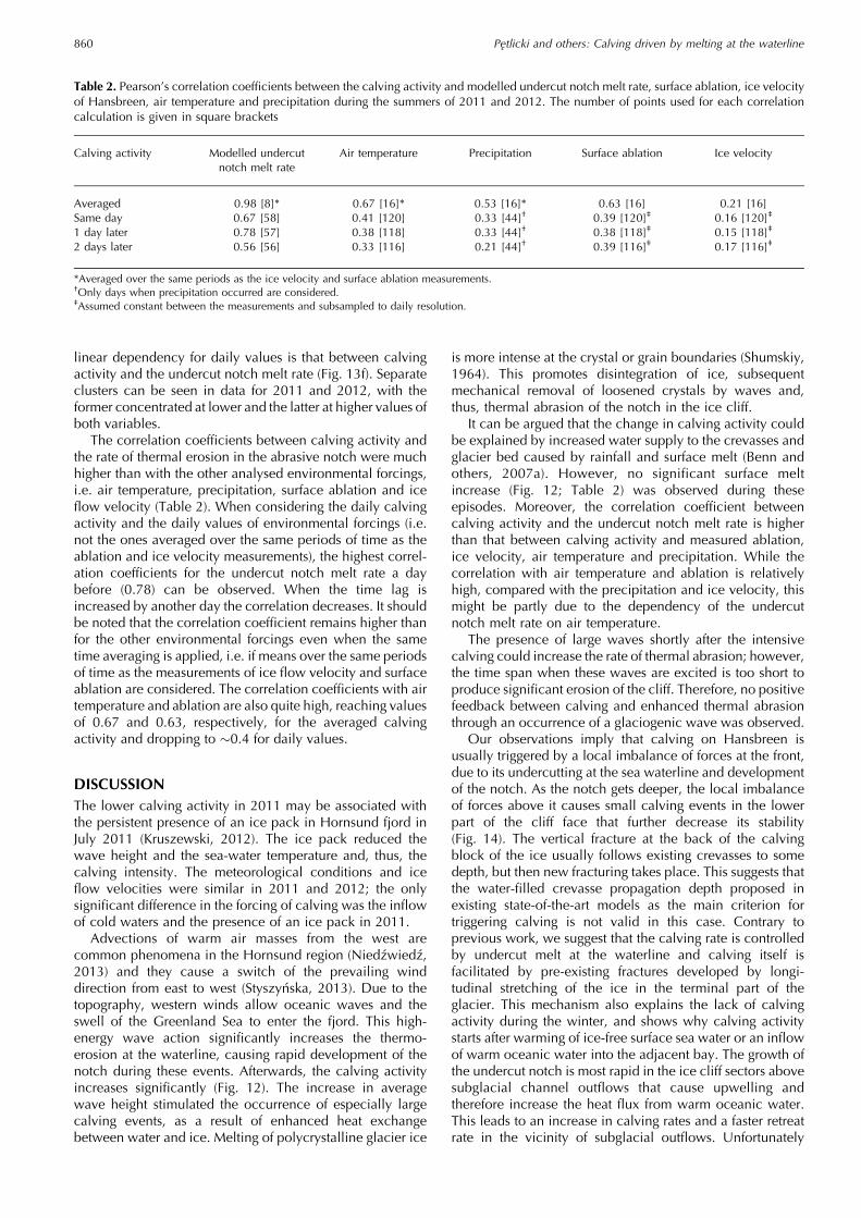
usually triggered by a local imbalance of forces at the front,due to its undercutting at the sea waterline and developmentof the notch. As the notch gets deeper, the local imbalanceof forces above it causes small calving events in the lowerpart of the cliff face that further decrease its stability(Fig. 14). The vertical fracture at the back of the calvingblock of the ice usually follows existing crevasses to somedepth, but then new fracturing takes place. This suggests thatthe water-filled crevasse propagation depth proposed inexisting state-of-the-art models as the main criterion fortriggering calving is not valid in this case. Contrary toprevious work, we suggest that the calving rate is controlledby undercut melt at the waterline and calving itself isfacilitated by pre-existing fractures developed by longi-tudinal stretching of the ice in the terminal part of theglacier. This mechanism also explains the lack of calvingactivity during the winter, and shows why calving activitystarts after warming of ice-free surface sea water or an inflowof warm oceanic water into the adjacent bay. The growth ofthe undercut notch is most rapid in the ice cliff sectors abovesubglacial channel outflows that cause upwelling andtherefore increase the heat flux from warm oceanic water.This leads to an increase in calving rates and a faster retreatrate in the vicinity of subglacial outflows. Unfortunately

Table 2. Pearson’s correlation coefficients between the calving activity and modelled undercut notch melt rate, surface ablation, ice velocityof Hansbreen, air temperature and precipitation during the summers of 2011 and 2012. The number of points used for each correlationcalculation is given in square brackets

Calving activity Modelled undercutnotch melt rate

Air temperature Precipitation Surface ablation Ice velocity

Averaged 0.98 [8]* 0.67 [16]* 0.53 [16]* 0.63 [16] 0.21 [16]Same day 0.67 [58] 0.41 [120] 0.33 [44]† 0.39 [120]‡ 0.16 [120]‡

1 day later 0.78 [57] 0.38 [118] 0.33 [44]† 0.38 [118]‡ 0.15 [118]‡

2 days later 0.56 [56] 0.33 [116] 0.21 [44]† 0.39 [116]‡ 0.17 [116]‡

*Averaged over the same periods as the ice velocity and surface ablation measurements.†Only days when precipitation occurred are considered.‡Assumed constant between the measurements and subsampled to daily resolution.


insufficient data are available to provide a precise estimateof the increase of the melt rate in these areas of Hansbreen,but the presence of the ice gates above the subglacialoutflows shows this rate to be significant, although spatiallylimited to this specific area.An example of a detailed survey of a calving event on

31 July 2012 shows that the vertical profile of the ice cliffafter calving does not follow a strictly vertical shape(Fig. 11). The undercut notch depth before calving isapproximately equal to one-third of the depth of the calvedice block measured at the water level. The slope of the icecliff in the lower part then reverses, from overhanging tosloping towards the sea (Fig. 11). The lower part of the newice cliff surface shows clean blue ice, with no visible tracesof ablation, sediments or old snow trapped within thecrevasse during the winter. This contradicts the theory of themechanism of calving due to longitudinal stretching causedby the acceleration of ice near the front, where the crevassesopen gradually during ice flow towards the ice cliff.The discrepancies between the modelled (Fig. 9d) and

measured (Fig. 10b) undercut notch depths are significant.The maximum cumulative measured depth over the period31 July–19 August 2012 was 22% lower than the cumu-lative notch melt. The mean cumulative depth in thewesternmost sector of the ice cliff was 43% of the modelledvalue, whereas for the whole surveyed part of the cliff itwas only 23% (Figs 9d and 10b). It can be argued that thelower values of the undercut notch depth in the eastern partof the survey were caused by a poorer-quality return signal,i.e. lower intensity of the reflected laser beam due to thegreater distance to the ice cliff. These discrepancies can beexplained by two factors: underestimation of the measuredcumulative undercut notch depth, due to the low samplingrate and overestimation of the modelled melt rate, due toan imprecise parameterization of the model. The modelparameters (the empirical constant coefficient of 0.000146and the roughness length, R) need to be tuned to the localconditions if enough validation data are available. How-ever, given the large variation in the observed rate of notchcutting (Fig. 10), the high quality of the validation of theseparameters reported by El-Tahan and others (1987) and thatthey were kept unchanged in the work of Vieli and others(2002), it seemed most appropriate to apply this original setof parameters, to allow direct comparison of the modelresults with former studies. Obviously, this may be animportant source of the observed discrepancy between themodelled and measured melt rates; however, given thesimple form of the model (Eqn (1)) and a relatively smallamount of gathered observational data that could be usedto calibrate it, the parameters have not been changed.Nevertheless, as the relationships of the model are linear or

almost linear, this discrepancy should not change theinterpretation of the obtained results.The sensitivity analysis of the undercut notch melt model

shows that the melt was more sensitive to water temperaturechanges in 2011 and to wave height changes in 2012(Fig. 9). In summer 2011 the sea-surface temperature wasrelatively low and the waves were higher than in summer2012 (Fig. 7). Therefore �T was low, as Ta was close to Tfp.Given the linear relationship between the undercut meltrate, Vm, and �T (Eqn (1)), a relatively large change in �T,in this case �1°C, resulted in a substantial change in themodelled melt rate. The same pattern was predicted for themodel sensitivity to the wave height in 2012. This resultsuggests that calving rates are highly sensitive to sea-watertemperature changes when close to the freezing point.The undercut melt rates calculated in this study are lower

than the 1md–1 value proposed by Vieli and others (2002).The main reason is that here field measured values of thewater temperature, wave height and period were used,while Vieli and others only roughly estimated thesevariables. Another issue is that in the study of Vieli andothers (2002) the undercut melt rate was equal to the calvingrate caused by the imbalance of forces, due to theundercutting at water level, i.e. this type of calving wasassociated only with the break-off of ice slabs directly abovethe notch. Here we show that it can also trigger calvingevents at greater depth, even up to twice the undercut notchdepth. It could therefore be speculated that the calving ratesmight be equal to at least twice the melt rate of the undercut,which stays in accordance with the modelling studies(O’Leary and Christoffersen, 2013).The size and dynamics of Hansbreen are typical of a

Svalbard grounded tidewater glacier; however, it should benoted that the processes observed there may not besignificant for larger glaciers. This may be the case forfloating or semi-floating glaciers, where submarine melt atthe grounding line can trigger large calving events, which donot occur on smaller glaciers such as Hansbreen. Never-theless, undercutting at the waterline may be of greatimportance for calving of grounded tidewater glaciers ofcomparable size to Hansbreen.

CONCLUSIONSThe main conclusion of this study is that calving onHansbreen grounded tidewater glacier is mainly triggeredby the local imbalance of forces at the front, due toundercutting at the sea waterline and development of athermo-erosional notch. There is a strong correlationbetween the observed calving activity and the modelled icemelt at the waterline. This correlation is particularly strong

Fig. 14. Hansbreen ice cliff with small overhangs due to calving above the undercut notch (marked with C). Photograph taken using a time-lapse camera on 20 June 2010.


for a one-day lag between calving activity and the melt rate,indicating the importance of the mechanical destabilizationof the ice front by the undercut. A large part of the fracturingassociated with calving takes place just next to the calvingfront, which contradicts the theoretical mechanism ofgradual stretching of crevasses due to acceleration of iceflow in the frontal part, and their deepening by the presenceof water. In summer 2011 the presence of dense drifting sea-ice floes in Hornsund fjord drastically decreased the calvingintensity of Hansbreen, by cooling surface water andsuppressing wave action. Hansbreen and tidewater glaciersof the western coast of Svalbard are sensitive to atmosphericadvection from the west, due to the associated influx ofwarmer sea water and increased wave activity, causing morerapid development of the thermo-erosional notch at sea leveland, hence, calving. It can be expected that calving rates ofthe tidewater glaciers of Svalbard will rise with increasedadvection of warmer Atlantic waters to the Arctic.

AUTHOR CONTRIBUTION STATEMENTM.P. performed all calculations, collected TLS, ice velocityand mass-balance data and wrote most of the paper; M.C.investigated calving activity and surface sea-water proper-ties; J.A.J. designed the study of the undercut notch; A.P.provided CTD data and C.K. helped in writing this paper.

ACKNOWLEDGMENTSWe thank the crew of Polish Polar Station Hornsund for theirsupport with fieldwork. We also thank J. Abermann forvaluable comments that helped to improve the manuscript.The studies were partly funded by the statutory activity ofthe Institute of Geophysics, Polish Academy of Sciences,Polish National Science Center grant DEC-2013/11/N/ST10/00823, Polish–Norwegian Fund projects AWAKE (PNRF-22-AI-1/07) and AWAKE2 (Pol-Nor/198675/17/2013). Thepublication has been partially financed by the Centre forPolar Studies from the funds of the Leading NationalResearch Centre (KNOW) in Earth Sciences (2014–18).

REFERENCESAlley R, Dupont T, Parizek B and Anandakrishnan S (2005) Accessof surface meltwater to beds of sub-freezing glaciers: pre-liminary insights. Ann. Glaciol., 40, 8–14 (doi: 10.3189/172756405781813483)

Amundson J and Truffer M (2010) A unifying framework foriceberg-calving models. J. Glaciol., 56(199), 822–830 (doi:10.3189/002214310794457173)

Benn D, Warren C and Mottram R (2007a) Calving processes andthe dynamics of calving glaciers. Earth-Sci. Rev., 82, 143–179(doi: 10.1016/j.earscirev.2007.02.002)

Benn D, Hulton N and Mottram R (2007b) ‘Calving laws’, ‘slidinglaws’ and the stability of tidewater glaciers. Ann. Glaciol., 46,123–130 (doi: 10.3189/172756407782871161)

Blaszczyk M, Jania J and Hagen J (2009) Tidewater glaciers ofSvalbard: recent changes and estimates of calving fluxes. Pol.Polar Res., 30(2), 85–142

BlaszczykM, Jania J and Kolondra L (2013) Fluctuations of tidewaterglaciers in Hornsund Fjord (Southern Svalbard) since thebeginning of the 20th century. Pol. Polar Res., 34(4), 327–352(doi: 10.2478/popore-2013-0024)

Brown C, Meier M and Post A (1982) Calving speed of Alaskatidewater glaciers, with application to Columbia Glacier. USGSProf. Pap. 1258-C

Budd W, Jacka T and Morgan V (1980) Antarctic iceberg melt ratesderived from size distributions and movement rates. Ann.Glaciol., 1, 103–112

Chapuis A (2011) What controls the calving of glaciers? Fromobservations to predictions. (PhD thesis, Norwegian Universityof Life Sciences)

Chapuis A and Tetzlaff T (2014) The variability of tidewater-glacier calving: origin of event-size and interval distributions.J. Glaciol., 60(222), 622–634 (doi: 10.3189/2014JoG13J215)

Cottier F, Nilsen F, Skogseth R, Tverberg V, Skarðhamar J andSvendsen H (2010) Arctic fjords: a review of the oceanographicenvironment and dominant physical processes. Geol. Soc.London Spec. Publ., 344(1), 35–50 (doi: 10.1144/SP344.4)

Deems J, Painter T and Finnegan D (2013) Lidar measurements ofsnow depth: a review. J. Glaciol., 59(215), 467–479 (doi:10.3189/2013JoG12J154)

Eijpen K, Warren C and Benn D (2003) Subaqueous melt rates atcalving termini: a laboratory approach. Ann. Glaciol., 36,179–183 (doi: 10.3189/172756403781816158)

El-Tahan M, Venkatesh S and El-Tahan H (1987) Validation andquantitative assessment of the detoriation mechanisms of Arcticicebergs. J. Offshore Mech. Arct. Eng., 109, 102–108

Glazovsky A, Macheret Y, Moskalevsky M and Jania J (1991)Tidewater glaciers of Spitsbergen. IAHS Publ. 208 (Symposiumat St Petersburg 1990 – Glaciers–Ocean–Atmosphere Inter-actions), 229–240

Glowacki O, Deane G, Moskalik M, Blondel P, Tegowski J andBlaszczyk M (2015) Underwater acoustic signatures of glaciercalving. Geophys. Res. Lett., 42, 804–812 (doi: 10.1002/2014GL062859)

Grabiec M, Jania J, Puczko D and Kolondra L (2012) Surface andbed morphology of Hansbreen. Pol. Polar Res., 33(2), 111–138(doi: 10.2478/v10183-012-0010-7)

Haresign E (2004) Glacio-limnological interactions at lake-calvingglaciers. (PhD thesis, University of St Andrews)

Iken A (1977) Movement of a large ice mass before breaking off.J. Glaciol., 19(81), 595–604

Jania J (1988) Dynamiczne procesy glacjalne na południowymSpitsbergenie (w świetle badaņ„ fotointerpretacyjnych i foto-grametrycznych) [Dynamic glacial processes in southern Spits-bergen (in the light of photointerpretation and photogrammetricresearch)]. University of Silesia, Katowice

Jania J, Mochnacki D and Gadek B (1996) The thermal structure ofHansbreen, a tidewater glacier in southern Spitsbergen,Svalbard. Polar Res., 15(1), 53–66

Jenkins A (2011) Convection-driven melting near the groundinglines of ice shelves and tidewater glaciers. J. Phys. Oceanogr.,41(12), 2279–2294 (doi: 10.1175/JPO-D-11-03.1)

Josberger E (1983) Sea ice melting in the marginal ice zone.J. Geophys. Res., 88(C5), 2841–2844

Josberger E and Martin S (1981) A laboratory and theoretical studyof the boundary layer adjacent to a vertical melting ice wall insalt water. J. Fluid Mech., 111, 439–473

Joughin I, Abdalati W and Fahnestock M (2004) Large fluctuationsin speed on Greenland’s Jakobshavn Isbræ glacier. Nature,432(7017), 608–610 (doi: 10.1038/nature03130)

Kirkbride M and Warren C (1997) Calving processes at a groundedice cliff. Ann. Glaciol., 24, 116–121

Köhler A, Chapuis A, Nuth C, Kohler J and Weidle C (2012)Autonomous detection of calving-related seismicity at Krone-breen, Svalbard. Cryosphere, 6(2), 393–406 (doi: 10.5194/tc-6-393-2012)

Kruszewski G (2012) Zlodzenie Hornsundu i wód przyległych(Spitsbergen) w sezonie zimowym 2010–2011. [Ice conditionsin Hornsund and adjacent waters (Spitsbergen) during winterseason 2010–2011]. Probl. Klimatol. Pol., 22, 69–82

Kruszewski G (2013) Zlodzenie Hornsundu i wód przyległych(Spitsbergen) w sezonie zimowym 2011–2012. [Ice conditions inHornsund and adjacentwaters (Spitsbergen) duringwinter season2011–2012]. Probl. Klimatol. Pol., 23, 169–179


Lapazaran J and 6 others (2013) Ice volume changes (1936–1990–2007) and ground-penetrating radar studies of Ariebreen,Hornsund, Spitsbergen. Polar Res., 32, 11 068 (doi: 10.3402/polar.v32i0.11068)

Mansell D, Luckman A and Murray T (2012) Dynamics of tidewatersurge-type glaciers in northwest Svalbard. J. Glaciol., 58,110–118 (doi: 10.3189/2012JoG11J058)

Marsz A and Styszyńska A (2013) Climate and climate change atHornsund, Svalbard. Gdynia Maritime University, Gdynia

Meier M and Post A (1987) Fast tidewater glaciers. J. Geophys. Res.,92(B9), 9051–9058 (doi: 10.1029/JB092iB09p09051)

Motyka R, Hunter L, Echelmeyer K and Connor C (2003) Submarinemelting at the terminus of a temperate tidewater glacier,LeConte Glacier, Alaska, USA. Ann. Glaciol., 36(1), 57–65(doi: 10.3189/172756403781816374)

Motyka R, Dryer W, Amundson J, Truffer M and Fahnestock M(2013) Rapid submarine melting driven by subglacial dis-charge, LeConte Glacier, Alaska. Geophys. Res. Lett., 40(19),5153–5158 (doi: 10.1002/grl.51011)

Murray T and 9 others (2015) Dynamics of glacier calving at theungrounded margin of Helheim Glacier, South-East Greenland.J. Geophys. Res. Earth Surf., 120 (doi: 10.1002/2015JF003531)

Nick F, Van der Veen C, Vieli A and Benn D (2010) A physicallybased calving model applied to marine outlet glaciers and impli-cations for the glacier dynamics. J. Glaciol., 56(199), 781–794(doi: 10.3189/002214310794457344)

Niedźwiedź T (2013) The atmospheric circulation. In Marsz A andStyszyńska A eds Climate and climate change at Hornsund,Svalbard. Gdynia Maritime University, Gdynia, 57–74

Nuth C and 7 others (2013) Decadal changes from a multi-temporalglacier inventory of Svalbard. Cryosphere, 7(5), 1603–1621(doi: 10.5194/tc-7-1603-2013)

Nye J (1955) Correspondence. Comments on Dr Loewe’s letter andnotes on crevasses. J. Glaciol., 2(17), 512–514

Nye J (1957) The distribution of stress and velocity in glaciers andice-sheets. Proc. R. Soc. London, 239(1216), 113–133

Oerlemans J, Jania J and Kolondra L (2011) Application of aminimal glacier model to Hansbreen, Svalbard. Cryosphere,5(1), 1–11 (doi: 10.5194/tc-5-1-2011)

O’Leary M and Christoffersen P (2013) Calving on tidewater glacieramplified by submarine frontal melting. Cryosphere, 7, 119–128

O’Neel S, Echelmeyer K and Motyka R (2003) Short-termvariations in calving of a tidewater glacier: LeConte Glacier,Alaska. J. Glaciol., 49(167), 587–598 (doi: 10.3189/172756503781830430)

O’Neel S, Larsen C, Rupert N and Hansen R (2010) Iceberg calvingas a primary source of regional-scale glacier-generated seismi-city in the St Elias Mountains, Alaska. J. Geophys. Res., 115(F4),F04034 (doi: 10.1029/2009JF001598)

Otero J, Navarro F, Martin C, Cuadrado M and Corcuera M (2010)A three-dimensional calving model: numerical experiments onJohnsons Glacier, Livingston Island, Antarctica. J. Glaciol.,56(196), 200–214 (doi: 10.3189/002214310791968539)

Pelto M and Warren C (1991) Relationship between tidewaterglacier calving velocity and water depth at the calving front.Ann. Glaciol., 15, 115–118

Pettit E (2012) Passive underwater acoustic evolution of acalving event. Ann. Glaciol., 53(60), 113–122 (doi: 10.3189/2012AoG60A137)

Polish Polar Station, Institute of Geophysics Polish Academy ofSciences (2011) Summary of the year 2011. MeteorologicalBulletin, Spitsbergen–Hornsund

Polish Polar Station, Institute of Geophysics Polish Academy ofSciences (2012) Summary of the year 2012. MeteorologicalBulletin, Spitsbergen–Hornsund

Prokop A (2008) Assessing the applicability of terrestrial laserscanning for spatial snow depth measurements. Cold Reg. Sci.Technol., 54(3), 155–163 (doi: 10.1016/j.coldregions.2008.07.002)

Rivera A, Corripio J, Bravo C and Cisternas S (2012) Glaciar JorgeMontt (Chilean Patagonia) dynamics derived from photos ob-tained by fixed camera and satellite image feature tracking. Ann.Glaciol., 53(60), 147–155 (doi: 10.3189/2012AoG60A152)

Rohl K (2006) Thermo-erosional notch development at fresh-water-calving Tasman Glacier, New Zealand. J. Glaciol., 52(177),203–213 (doi: 10.3189/172756506781828773)

Ryan J and 7 others (2015) UAV photogrammetry and structurefrom motion to assess calving dynamics at Store Glacier, a largeoutlet draining the Greenland ice sheet. Cryosphere, 9(1), 1–11(doi: 10.5194/tc-9-1-2015)

Schlitzer R (2015) Ocean data view. http://odv.awi.deShumskiy P (1964) Principles of structural glaciology. Translatedfrom the Russian by D. Kraus. Dover, New York (originalpublication 1955)

Sikonia W (1982) Finite-element glacier dynamics model applied toColumbia Glacier, Alaska. USGS Prof. Pap. 1258-B

Styszyńska A (2013) The winds. In Marsz A and Styszyńska A edsClimate and climate change at Hornsund, Svalbard. GdyniaMaritime University, Gdynia, 81–100

Van der Veen C (1998) Fracture mechanics approach to penetrationof surface crevasses on glaciers. Cold Reg. Sci. Technol., 27(1),31–47 (doi: 10.1016/S0165-232X(97)00022-0)

Van der Veen C (2002) Calving glaciers. Progr. Phys. Geogr., 26(1),96–122 (doi: 10.1191/0309133302pp327ra)

Venteris E (1999) Rapid tidewater glacier retreat: a comparisonbetween Columbia Glacier, Alaska and Patagonian calvingglaciers. Global Planet. Change, 22(1–4), 131–138 (doi:10.1016/S0921-8181(99)00031-4)

Vieli A, Funk M and Blatter H (2001) Flow dynamics of tidewaterglaciers: a numerical modelling approach. J. Glaciol., 47(159),595–606 (doi: 10.3189/172756501781831747)

Vieli A, Jania J and Kolondra L (2002) The retreat of a tidewaterglacier: observations and model calculations on Hansbreen,Spitsbergen. J. Glaciol., 48(163), 592–600 (doi: 10.3189/172756502781831089)

Walczowski W and Piechura J (2011) Influence of the WestSpitsbergen Current on the local climate. Int. J. Climatol., 31(7),1088–1093 (doi: 10.1002/joc.2338)

Weertman J (1973) Can a water filled crevasse reach the bottomsurface of a glacier? IAHS Publ. 95 (Symposium at Reading 1970– World Water Balance), vol. 2, 139–145

Westoby M, Brasington J, Glasser N, Hambrey M and Reynolds J(2012) ‘Structure-from-motion’ photogrammetry: a low-cost,effective tool for geoscience applications. Geomorphology,179, 300–314 (doi: 10.1016/j.geomorph.2012.08.021)

White F, SpauldingMandGominho L (1980) Theoretical estimates ofthe various mechanisms involved in iceberg deterioration in theopen ocean environment. US Coast Guard Rep. CG-D-62-80

MS received 7 May 2015 and accepted in revised form 19 June 2015


Documents

Calving of a tidewater glacier driven by melting at the ... · Calving of a tidewater glacier driven by melting at ... We present a study of the development of a thermo-erosional