Calving controlled by melt-under-cutting: detailed calving ......maxima occurring in 1930, 1971, 2004 (Flink and others, 2015) and most recently in 2016 (A. Luckman, pers. comm.)

Calving controlled by melt-under-cutting: detailed calving stylesrevealed through time-lapse observations

Penelope HOW,1,2* Kristin M. SCHILD,3,4 Douglas I. BENN,5 Riko NOORMETS,2

Nina KIRCHNER,6 Adrian LUCKMAN,7,8 Dorothée VALLOT,9

Nicholas R. J. HULTON,1,2 Chris BORSTAD8

1Institute of Geography, School of GeoSciences, University of Edinburgh, Edinburgh, UKE-mail: [email protected]

2Department of Arctic Geology, University Centre in Svalbard, Longyearbyen, Norway3Department of Earth Sciences, University of Oregon, Eugene, USA

4Climate Change Institute, University of Maine, Orono, USA5Department of Geography and Sustainable Development, University of St. Andrews, Fife, UK

6Department of Physical Geography, Stockholm University, Stockholm, Sweden7Department of Geography, College of Science, Swansea University, Swansea, UK

8Department of Arctic Geophysics, University Centre in Svalbard, Longyearbyen, Norway9Department of Earth Sciences, Uppsala University, Uppsala, Sweden

ABSTRACT. We present a highly detailed study of calving dynamics at Tunabreen, a tidewater glacier inSvalbard. A time-lapse camera was trained on the terminus and programmed to capture images every 3seconds over a 28-hour period in August 2015, producing a highly detailed record of 34 117 images fromwhich 358 individual calving events were distinguished. Calving activity is characterised by frequentevents (12.8 events h−1) that are small relative to the spectrum of calving events observed, demonstrat-ing the prevalence of small-scale calving mechanisms. Five calving styles were observed, with a high pro-portion of calving events (82%) originating at, or above, the waterline. The tidal cycle plays a key role inthe timing of calving events, with 68% occurring on the falling limb of the tide. Calving activity is con-centrated where meltwater plumes surface at the glacier front, and a ∼ 5 m undercut at the base of theglacier suggests that meltwater plumes encourage melt-under-cutting. We conclude that frontal ablationat Tunabreen may be paced by submarine melt rates, as suggested from similar observations at glaciers inSvalbard and Alaska. Using submarine melt rate to calculate frontal ablation would greatly simplify esti-mations of tidewater glacier losses in prognostic models.

Keywords: Arctic glaciology, glacier calving, ice dynamics, ice/ocean interactions

INTRODUCTIONThe loss of ice from the termini of marine-terminating glaciers(i.e. frontal ablation) occurs by both submarine melting andiceberg calving. Calving from tidewater glaciers can occurby a number of mechanisms, including longitudinal stretch-ing, buoyant instability and under-cutting of the front by sub-marine melt (Van Der Veen, 2002; Benn and others, 2007).Submarine melting can influence calving by under-cuttingand destabilising the subaerial part of the ice front. Studieson several glaciers indicate that submarine melting is animportant process in settings where relatively warm oceanwater interacts with glacier fronts, and efficient heat transferis promoted by buoyant meltwater plumes (Motyka andothers, 2003; Bartholomaus and others, 2013; Chauchéand others, 2014; Rignot and others, 2015; Slater andothers, 2015; Truffer and Motyka, 2016).

Where melt-under-cutting is the dominant driver ofcalving, frontal ablation rates depend on the relationshipbetween two fundamental factors: (1) the temporal andspatial evolution of subaqueous cavities by melting; and (2)the mechanical response of the ice to the evolving geometryand associated stresses (Joughin and others, 2008; Howat

and others, 2010). Although important observations havebeen made about the morphology of undercut cavities(e.g., Rignot and others, 2015), there is a lack of concurrentdata on cavity development and calving events. Our under-standing of the relationship between under-cutting andcalving is, therefore, heavily reliant on modelling at present.

Melting of submerged ice is a function of water temperatureand tangential velocity (Holland and others, 2008; Straneoand others, 2010; Jenkins, 2011). The motion of water up oracross an ice front can occur as the result of wind-driven, tidaland other currents (e.g., Bartholomaus and others, 2013;Sutherland and others, 2014; Petlicki and others, 2015; Schildand others, 2018), or convection driven by the ascent ofbuoyant meltwater (e.g., Schild and others, 2016). Plumes ofmeltwater rising from subglacial discharge points and plume-driven secondary circulation patterns are considered to playparticularly important roles in submarine melting and melt-under-cutting (e.g., Cowton and others, 2015; Slater and others,2017a,b; Schild and others, 2018; Vallot and others, 2018a).

Experiments with the discrete element model HiDEM(Benn and others, 2017; Vallot and others, 2018a) suggestthat calving can occur in response to melt-under-cutting intwo distinct ways: (1) where undercuts are small, low-magnitude calving can occur via localised collapse of theoverhang; and (2) where undercuts are large, high-magnitude

*Present address: Department of Environment and Geography, University ofYork, York, UK.

Annals of Glaciology 60(78) 2019 doi: 10.1017/aog.2018.28 20© The Author(s) 2019. This is an Open Access article, distributed under the terms of the Creative Commons Attribution licence (http://creativecommons.org/licenses/by/4.0/), which permits unrestricted re-use, distribution, and reproduction in any medium, provided the original work is properly cited.

Downloaded from https://www.cambridge.org/core. 09 Jul 2020 at 14:47:21, subject to the Cambridge Core terms of use.

mailto:[email protected]

https://www.cambridge.org/core

calving events can remove all of the overhang plus additionalice. In the latter case, fractures form at the ice surface upgla-cier of the undercut, and propagate downwards as the icefront bends forward and downward. These contrastingresponses to under-cutting have important implications forlong-term calving rates. If undercuts are able to grow largeenough to trigger high-magnitude calving events, long-termcalving rates will be greater than the submarine melt rate(i.e. the calving multiplier effect proposed by O’Leary andChristoffersen, 2013). On the contrary, if low-magnitudecalving events prevent undercuts from becoming largeenough to trigger high-magnitude calving, long-termcalving rates will simply equal the under-cutting rate. Thisanalysis suggests that the relationship between melt-under-cutting and calving can be inferred from detailed observa-tions of calving events, especially calving style.

The magnitude, frequency, and style of calving events areintrinsically linked. Calving activity can range from verysmall (<104 m3) and frequent (>100 d−1) events, to larger(>108 m3) and infrequent (<1 d−1) occurrences (Åströmand others, 2014; Chapuis and Tetzlaff, 2014). Many large,infrequent calving events have been identified using time-lapse photography (e.g., Rosenau and others, 2013; Jamesand others, 2014; Medrzycka and others, 2016). Thecalving styles associated with smaller, more frequent eventsare challenging to document because small calved bergsare difficult to distinguish in satellite images and low-tem-poral time-lapse photography. Under-representation ofsmall-scale calving styles, and their control over long-termfrontal ablation is, therefore, an inherent problem.

Here, we examine calving dynamics at Tunabreen, a tide-water glacier in Svalbard, where calving activity is known tobe low-magnitude and frequent (Köhler and others, 2015;Luckman and others, 2015). A time-lapse camera was installedon a ridge adjacent to the glacier terminus, capturing imagesevery 3 seconds (Fig. 1a). This produced a highly detailedrecord of calving events over a period of 28 hours during 7–8August 2015. Taken together with bathymetric surveys of theseabed/submarine icecliff andobservationsofplume locations,this record allows us to study the processes associatedwith indi-vidual calving events and the role of melt-under-cutting.

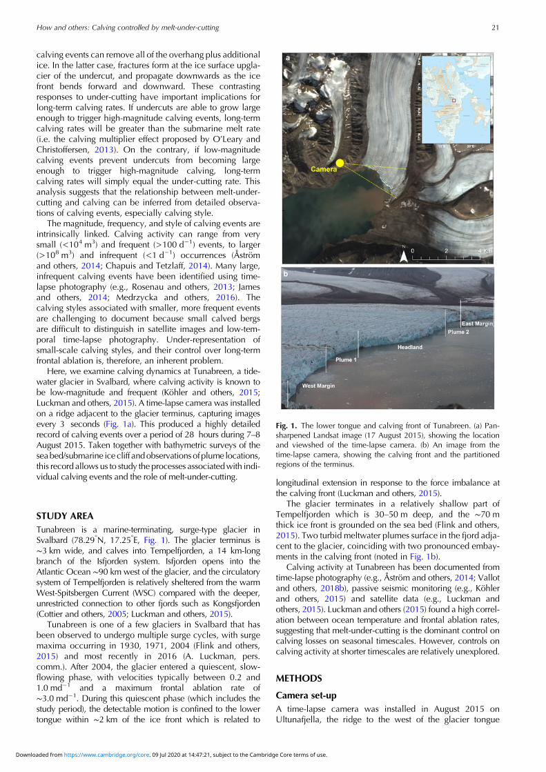
STUDY AREATunabreen is a marine-terminating, surge-type glacier inSvalbard (78.29°N, 17.25°E, Fig. 1). The glacier terminus is∼3 km wide, and calves into Tempelfjorden, a 14 km-longbranch of the Isfjorden system. Isfjorden opens into theAtlantic Ocean ∼90 km west of the glacier, and the circulatorysystem of Tempelfjorden is relatively sheltered from the warmWest-Spitsbergen Current (WSC) compared with the deeper,unrestricted connection to other fjords such as Kongsfjorden(Cottier and others, 2005; Luckman and others, 2015).

Tunabreen is one of a few glaciers in Svalbard that hasbeen observed to undergo multiple surge cycles, with surgemaxima occurring in 1930, 1971, 2004 (Flink and others,2015) and most recently in 2016 (A. Luckman, pers.comm.). After 2004, the glacier entered a quiescent, slow-flowing phase, with velocities typically between 0.2 and1.0 md−1 and a maximum frontal ablation rate of∼3.0 md−1. During this quiescent phase (which includes thestudy period), the detectable motion is confined to the lowertongue within ∼2 km of the ice front which is related to

longitudinal extension in response to the force imbalance atthe calving front (Luckman and others, 2015).

The glacier terminates in a relatively shallow part ofTempelfjorden which is 30–50 m deep, and the ∼70 mthick ice front is grounded on the sea bed (Flink and others,2015). Two turbid meltwater plumes surface in the fjord adja-cent to the glacier, coinciding with two pronounced embay-ments in the calving front (noted in Fig. 1b).

Calving activity at Tunabreen has been documented fromtime-lapse photography (e.g., Åström and others, 2014; Vallotand others, 2018b), passive seismic monitoring (e.g., Köhlerand others, 2015) and satellite data (e.g., Luckman andothers, 2015). Luckman and others (2015) found a high correl-ation between ocean temperature and frontal ablation rates,suggesting that melt-under-cutting is the dominant control oncalving losses on seasonal timescales. However, controls oncalving activity at shorter timescales are relatively unexplored.

METHODS

Camera set-upA time-lapse camera was installed in August 2015 onUltunafjella, the ridge to the west of the glacier tongue

Fig. 1. The lower tongue and calving front of Tunabreen. (a) Pan-sharpened Landsat image (17 August 2015), showing the locationand viewshed of the time-lapse camera. (b) An image from thetime-lapse camera, showing the calving front and the partitionedregions of the terminus.

21How and others: Calving controlled by melt-under-cutting



(Fig. 1a). The system consisted of a Canon EOS 700D camerabody, an EF 50 mm f/1.8 II fixed focal lens and aHarbortronics Digisnap 2700 intervalometer, which waspowered by a 12 V DC battery and a 10 W solar panel.The camera was set to take one photo every 3 seconds, pro-ducing a record that spans a 28-hour period from 19:25 onthe 7 August to 23:53 on the 8 August (local time,GMT+2). Images were taken using shutter-priority settingsbecause it was important to capture images across a consist-ent time window (rather than use aperture-priority settings toachieve a consistent light level). Each image was time-stamped by the clock on the camera. Camera clock drift isa common problem in time-lapse photogrammetry and it isdifficult to overcome this limitation without a direct connec-tion to an accurate clock, such as a GPS (Welty and others,2013). The clock on the camera at Tunabreen drifted by ∼2seconds over the course of the monitoring period, based onthe drift in the time stamp. This drift was corrected for inpost-processing.

Calving styleIn all, 34 117 images were collected, and the style of eachcalving event was manually determined by examining thetime-lapse imagery on a frame-by-frame basis. Each eventwas noted for the origin of the collapsing ice (i.e. subaerialor subaqueous), the source of failure in the ice column, andthe amount of rotation in the falling section. Calving eventswere subsequently grouped into five classes: waterlineevent, ice-fall event, sheet collapse, stack topple, and sub-aqueous events (Table 1). These characterisations arebased on those outlined in previous studies (e.g., Bennand others, 2007; O’Neel and others, 2007; Bartholomausand others, 2012; Chapuis and Tetzlaff, 2014; Benn andothers, 2017; Minowa and others, 2018). The compiledvideo of the time-lapse imagery and the list of recordedcalving events are included as supplementary material inthis study.

Location of calving eventsThe calving front was divided into five sections based on keyterminus conditions: (1) the west margin, which is closest tothe camera and 660 m wide (determined from the satelliteimage is shown in Fig. 1a); (2) the first plume embayment(named Plume 1), which is 510 m wide; (3) the central head-land area, which is 900 m wide; (4) the second plumeembayment (named Plume 2), which is 390 m wide; and(5) the east margin, which is furthest away from the cameraand 470 m wide (Fig. 1b). The location of each calving

event was distinguished manually in the image plane andaffiliated with one of these regions.

In addition, the pixel (uv) locations in the image planewere translated to real-world xyz coordinates using the geor-ectification functions available in PyTrx. PyTrx (short for‘Python Tracking’) is an open source photogrammetrytoolbox for obtaining measurements from oblique imagery(How and others, 2018). The PyTrx toolbox predominantlyutilises functions from the OpenCV computer visiontoolbox (opencv.org), and its georectification tools are basedon those available in ImGRAFT (imgraft.glaciology.net)(Messerli and Grinsted, 2015). PyTrx is hosted on GitHub(github.com/PennyHow/PyTrx) along with the raw data andprocessing chains for deriving the xyz coordinates.

Several pieces of information were needed to translate theimage plane to three-dimensional space. A DEMwas acquiredfrom TanDEM-X in 2012, with a 10 m spatial resolution. Thecamera location was surveyed using a Trimble GeoXR GPSrover, which was linked to an SPS855 base station. Positionswere differentially post-processed to obtain a horizontal andvertical positional accuracy of 1.20 and 1.91 m, respectively.Ground control points (GCPs) were created from known xyzlocations in the camera field-of-view (e.g. features on the adja-cent mountain side). Intrinsic matrices and lens distortionparameters were calculated using the camera calibration func-tions available in the Matlab Computer Vision SystemToolbox. The georectified xyz coordinates have an error esti-mate of 5%, based on uncertainties in the camera parameters(How and others, 2017).

Surface velocitiesSurface velocities across the glacier terminus were derived byfeature-tracking a pair of TerraSAR-X Synthetic ApertureRadar (SAR) images, at 2 m spatial resolution, collected onthe 31 July and 11 August 2015. Feature tracking wasapplied to the image pair using a 200 pixel × 200 pixel cor-relation window (400 m × 400 m), with an uncertainty esti-mate of <0.4 m d−1 (as in Luckman and others, 2015).Averages for each region are calculated from these surfacevelocities, which are used in subsequent analysis.

Velocities could not be determined photogrammetricallyfrom the time-lapse images given that: (1) the glacier is rela-tively slow-flowing compared with other tidewater outlets inSvalbard; (2) the monitoring period is short which makes itdifficult to distinguish small displacements at the glaciersurface; and (3) it was difficult to derive velocities with lowerrors due to the oblique angle of the camera to glacierflow. These factors affected the signal-to-noise ratio in

Table 1. Calving styles observed at Tunabreen

Style category Details

Ice-fall event Small–medium size; typically involves a section of ice breaking off from the subaerial part of the ice front; tend to create a largesplash.

Sheet collapse Medium–large size; ice collapse has little or no rotation, likely to be facilitated by weaknesses at/near the waterline.Stack topple Medium–large size; ice collapse rotates outward from ice front indicating an outward force imbalance; failure usually occurs

through crevasse propagation.Waterline event Small size; small pieces of ice break off at the waterline, normally below or above an undercut section of the ice front; typically

generate little noise or splash.Subaqueousevent

Small–large size; ice breaks off from below the waterline and rises to the fjord surface.

22 How and others: Calving controlled by melt-under-cutting


http://opencv.org

http://imgraft.glaciology.net

https://github.com/PennyHow/PyTrx


photogrammetric processing, which meant that precise vel-ocity measurements could not be calculated. Therefore, sat-ellite-derived glacier surface velocities were the most robustoption for this monitoring period.

Conductivity, temperature and depth measurementsConductivity, temperature and depth (CTD) water measure-ments were collected in front of the glacier terminus on the10, 13 and 14 August. Specifically, temperature and conduct-ivity readings (fromwhich salinity measurements were derived)were collected at the fjord surface and at depths of 2.5, 5, 7.5,10, and 12.5 m below sea level (b.s.l.) (Schild, 2017). All ofthese measurements (including the location of each spot meas-urement) are included as supplementary material. Mean valueswere calculated from these to provide a general overview ofthe fjord conditions at the time of this study.

Bathymetric dataThe seafloor and ice front morphology were mapped using theKongsberg EM2040 multibeam echosounder, which wasmounted on the 15 m research vessel ‘Viking Explorer’.These surveys were undertaken on 3–5 August, and the 14August 2015. The survey collected on the 14th August is pre-sented subsequently because it has the best coverage of allthe datasets.

The echosounder has a 0.4° × 0.7° wide beam configur-ation and the slow survey speeds at the ice front resulted invery high sounding density (hundreds of datapoints persquare metre). This allowed generation of digital elevationgrids with up to 1 m isometric cell size. Data were processedand visualised using the QPS Fledermaus and GlobalMappersoftware packages.

Additional oceanic and atmospheric measurementsTidal level data were obtained from the Norwegian MappingAuthority Hydrographic Service, with measurementsrecorded every 10 minutes (kartverket.no). The tidal levelwas observed at Ny Ålesund, and adjusted for location (bya multiplication factor of 1.13) and time (minus 17 minutes)to represent water levels in Tempelfjorden. These correctionsare according to the tidal model used by the NorwegianMapping Authority Hydrographic Service.

Air temperature measurements were obtained from theweather station situated in Adventdalen, which is managedby the University Centre in Svalbard (www.unis.no/resources/weather-stations/). The original data were recordedat one second intervals, but for clarity, we present 10-minuteaverages. Although the Adventdalen weather station islocated ∼40 km WSW of Tunabreen, it provides a good esti-mation of the daily temperature cycle under the prevailingsynoptic conditions.

RESULTS

Calving styleFive styles of calving were observed within the 28-hour mon-itoring period: waterline events, ice-fall events, sheet col-lapses, stack topples and subaqueous events (Table 1). Thecalving front was visible over the course of the entire moni-toring period due to the midnight sun and optimal weatherconditions, and in total, 358 calving events were recorded.

Waterline and ice-fall events were typically the smallest,whilst sheet and stack topples were the largest (Table 1).These four types of calving events occurred in the subaerialsection of the ice front, above the waterline. Subaqueouscalving styles involved the break-off of ice from beneaththe waterline, producing large, dirty icebergs.

Waterline events occurred at, or just above, the waterline(Fig. 2a), resulting in under-cutting at the base of the subaerialpart of the ice column. Often these events were very small,producing little splash. It is likely that this style of calvingevent would be undetected by remote seismic monitoring(e.g., Köhler and others, 2015; How, 2018), requiring mul-tiple seismic installations at the glacier terminus in order toincrease the chance of detection (e.g., Bartholomaus andothers, 2015).

Ice-fall events are typified as the break-off of small/mediumchunks of ice across the subaerial part of the ice front (Fig. 2b).These occurred at all heights in the ice column, with thebreak-off of ice from the top of the ice column being easiestto detect because they produced the largest splash. Ice-fallswere observed to collapse as a whole body of ice, or disinte-grate before they hit the fjord water (Fig. 2b).

Sheet collapses consist of large detachments of ice fromthe terminus (Fig. 2c), where the body of ice collapses down-wards with little rotation, hence it looks like a sheet as itenters the fjord water. This can often affect a sizeableportion of the glacier front where melt-under-cutting and/orturbulence generated by wave action is apparent (O’Learyand Christoffersen, 2013; Petlicki and others, 2015).

Stack topples are another large calving style observed atTunabreen (Fig. 2d). Failure in the ice column originatesfrom above the waterline, causing large tabular columns ofice to collapse into the fjord water. Rotation in the fallingsection of ice was observed, rotating out from the glacierfront and often exploding on impact and generating ice bal-listics that were scattered across the fjord.

Subaqueous calving events occurred below the waterline(Fig. 2e). Although iceberg detachment from the glaciercould not be directly observed from the time-lapse cameraimagery, we could identify subaqueous calving events fromthe sudden emergence of icebergs in front of the glacier.Subaqueous events were the least common style of calving,but often produced large icebergs that were heavily freightedwith debris. These bergs typically have a dark or deep blueappearance, due to smooth surfaces associated with submar-ine melt (in contrast, subaerial ice surfaces are typicallyrough and appear white). Observations of debris-rich iceexposed in stranded bergs and ice cliffs during the wintermonths show abundant evidence of basal transport andshear (Lovell and others, 2015); and we conclude that thedebris-rich ice observed in subaqueously calved bergs origi-nated at, or close to, the base of the glacier similar to thosedescribed by Wagner and others (2014).

The majority of calving events (82%) were ice-fall andwaterline events, with 155 ice-fall events and 142 waterlineevents recorded over the monitoring period (Table 2). Sheetcollapses and stack topples comprised a smaller proportionof the recorded calving activity, with only 16 sheet collapsesand 14 stack topples recorded. Also, only 10 subaqueousevents occurred, but these often produced large icebergsthat upwelled into the fjord. Of the 358 detected calvingevents, 21 events could not be confidently classified fromthe time-lapse sequence. This was either due to poor visibil-ity at the waterline (due to the glare of the fjord surface) or



http://kartverket.no

https://www.unis.no/resources/weather-stations/

https://www.unis.no/resources/weather-stations/


partial concealment as a result of the time-lapse camera fieldof view.

Location of calving eventsCalving events occurred across the entire glacier front (Fig. 3),but were abundant in the central region of the terminus, with

84 observed events at Plume 1, 85 observed events in theheadland area, and 86 observed events at Plume 2 (Table 2).Fewer events were observed at the margins, with 62 observedevents at the west margin (i.e. closest to the camera), and 41events at the east margin (i.e. furthest away from the camera)(Fig. 1). The normalised values – calving spatial frequencyand calving-velocity ratio (Table 2) – were determined using

Fig. 2. Picture breakdown of calving styles observed at Tunabreen from 7 to 8 August 2015. The top image shows the full calving front withcolour-coded extents illustrating where subsequent calving events are located; (a) A waterline calving event; (b) An ice-fall calving eventoccurring from the top of the ice column;(c) A sheet collapse event where failure at the waterline causes the collapse of a large block ofoverhead ice; (d) A stack topple event where crevasse propagation causes a column of ice to rotate outwards from the terminus andcollapse; (e) A subaqueous calving event where ice detaches from the ice column below the waterline and upwells to the fjord surface.




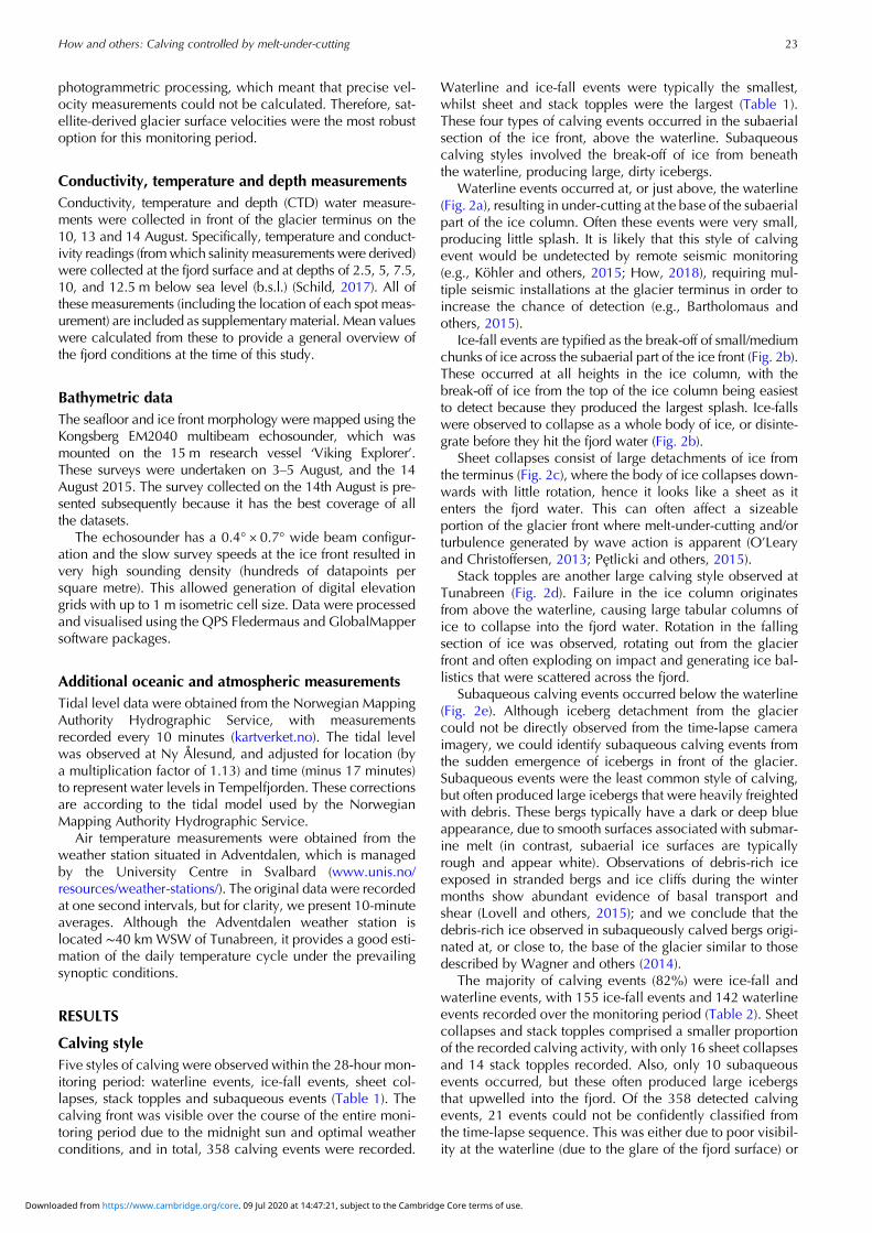
the width of each region of the terminus (as shown in Fig. 1b)and its average surface velocity, respectively. This shows thatwhilst there was consistent calving activity at the headlandand margin regions (0.09 calving events m−1), there wasfocused calving activity in the plume regions; with 0.17calving events m−1 at Plume 1 and 0.22 calving events m−1

at Plume 2. In addition, there is a disproportionate amountof calving at the margins despite slow surface velocities,which indicates that changes in velocity across the terminusare not linked to the total number of calving events observed.

Ice-fall events were the dominant style of calving at themargins of the terminus, with 31 recorded events at the westmargin and 30 at the east margin (Table 2). Abundant water-line events were also observed at the west margin, with 25recorded events (Table 2). Waterline events were the domin-ant calving style in the central regions of the terminus (Plume1,Headland, and Plume2 in Table 2). Ice-fall eventswere alsofrequent in these regions. The highest number of sheet col-lapses was observed at Plume 1 and the headland regions,with five recorded sheet collapses at Plume 1 and sevenrecorded sheet collapses in the headland region (Table 2).Stack topples occurred only in these two regions also (sevenevents occurring at Plume 1 and four events occurring in theheadland region, Table 2). Subaqueous events were observed

in the areas nearest to the time-lapse camera (i.e. the westmargin, Plume 1, and headland regions in Table 2),however, this could merely reflect the difficulty in detectingthis style of calving with distance from the camera.

Surface velocities (derived from TerraSAR-X imagery)ranged from 0 to ∼1 md−1 across the glacier terminusduring the monitoring period (Fig. 3b). The fastest flowingpart of the terminus is around the glacier centreline, encom-passing the two plumes and the headland region (defined inFig. 1b). These regions experienced the most calving events.In addition, stack topples occurred in Plume 1 and the head-land region, which are within the area of fastest flow.

Temporal distribution of calving eventsThe calving events are not randomly distributed in time butshow clear temporal patterns that allow environmental trig-gers to be identified. Air temperature measured at theAdventdalen weather station underwent small fluctuationsduring the observation period, ranging between 6.0 and9.1°C and peaking ∼16:00 (local time) on the 8 August(Fig. 4). This is typical of stable, clear-sky conditions duringthe Svalbard summer, when the sun is continuously abovethe horizon. Tidal levels fluctuated between 0.4 and 1.5 m,

Table 2. Calving events observed from the time-lapse image sequence (7–8 August 2015).

Calving style Area Total

West margin Plume 1 Headland Plume 2 East margin

Ice-fall event 31 30 31 33 30 155Sheet collapse 2 5 7 0 2 16Stack topple 0 7 4 3 0 14Waterline event 25 37 38 33 9 142Subaqueous event 2 4 4 0 0 10Unknown 2 1 0 17 0 21

Total 62 84 85 86 41 358Calving events m−1 width 0.09 0.17 0.09 0.22 0.09 –

Calving events m−1 d−1 140 111 101 216 363 –

Fig. 3. Calving events observed in the image plane (a) and georectified (b), with the colour of the point denoting the style of calving. Eventswere manually detected, from which the style of calving was interpreted. The time-lapse image was captured on the 8 August 04:36, and thesatellite image is a pan-sharpened Landsat image taken on the 17 August 2015.




with a tidal range of 1.1 m. The observation period spans alittle more than two tidal cycles.

Enhanced calving activity is evident between 08:00 and14:00 on the 8 August, coinciding with the falling limb (i.e.high-to-low) of the tidal cycle, with 111 events recorded incomparison with 29 events recorded on the prior risinglimb (02:00–08:00, 8 August). Of the two full tidal cyclesobserved during this monitoring period (from 19:40, 7August to 20:30, 8 August), 68% of calving activity (204events) occurred on the falling limbs of the tide and 32%(96 events) occurred on the rising limbs.

CTD measurementsCTD measurements taken in the fjord close to the glacierfront showed that warm, saline water was present belowdepths of 7.5 m b.s.l., with a mean temperature and salinityof ∼4.5°C and ∼32.6psu, respectively (Table 3). The waterat the surface is cooler (3.5°C) and fresher (18.9 psu) likelydue to meltwater runoff and/or floating bergs (Table 3).Temperature and salinity at intermediate depths shows

varying degrees of mixing between the surface water anddeeper layers.

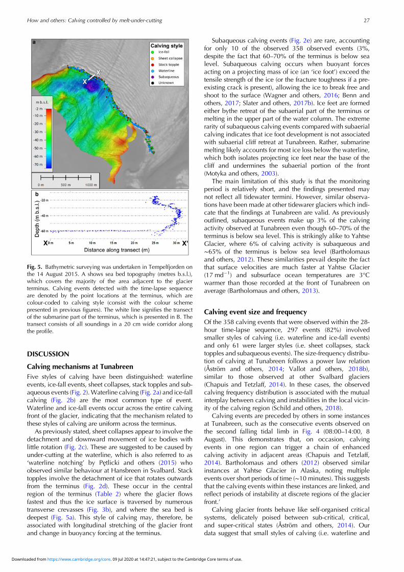
Bathymetric surveysThe bathymetric mapping of the sea floor covers an area of∼2 km2 across the majority of the fjord width (Fig. 5a). Theeast region of the fjord became very shallow (<10 m b.s.l.)hence why no data could be collected from the fjord wateradjacent to the east margin of the glacier. The sea bed topog-raphy ranged between 10 m and 70 m b.s.l., with relativelyshallow topography present at the boundaries of the surveyarea. An overdeepening is evident on the west side of thefjord, where topography was between 50 and 70 m b.s.l..This overdeepening is adjacent to the exit of one of the melt-water plumes from Tunabreen (with the glacier embaymentarea surrounding it referred to as Plume 1).

The echosounder was tilted in order to survey the submar-ine part of Tunabreen’s calving front in addition to the seabed survey. A transect of this is presented in Fig. 5b, whichwas taken in the Plume 1 region of the terminus (see whiteline in Fig. 5a for transect location). The transect in Fig. 5bdepicts all of the soundings along the profile as point mea-surements. The transect shows a ∼5 m undercut near theglacier bed. This undercut spans 35 m of the vertical submar-ine ice cliff (from a depth of 25 –60 m b.s.l. in Fig. 5b). Abovethis undercut is a near-vertical ice cliff, which is present froma depth of 25 m b.s.l. to the end of the transect (at a depth of10 m b.s.l.). This transect shows that there is substantialunder-cutting of the submarine ice cliff, which is likely tobe linked to the presence of a meltwater plume (Fried andothers, 2015). In comparing the detected calving events,we find stack topples, sheet collapses and subaqueousevents commonly occur in areas where the ice margin isseverely undercut, whereas waterline and small ice fallevents are common to the entire ice face (Fig. 5a).

Fig. 4. Space-time plot of the observed calving events, tidal level, and average air temperature. The colour of the point denotes the style ofcalving. The white and grey shaded regions represent the rising and falling tidal limb, respectively

Table 3. Average CTD measurements taken in front of Tunabreenon the 10, 13 and 14 August 2015

Depth Temperature(°C)*

Conductivity(μ S /cm−1)†

Salinity(psu)‡

Surface 3.52 17993 18.642.5 m 3.76 29344 30.625.0 m 4.03 30410 31.637.5 m 4.40 31312 32.3810.0 m 4.55 31730 32.7312.5 m 4.57 31814 32.79

* Temperature readings have an error estimate of ±0.2°C.† Conductivity measurements have an error estimate of ±2.0%.‡ Salinity measurements have an error estimate of ±1.0%.




DISCUSSION

Calving mechanisms at TunabreenFive styles of calving have been distinguished: waterlineevents, ice-fall events, sheet collapses, stack topples and sub-aqueous events (Fig. 2).Waterline calving (Fig. 2a) and ice-fallcalving (Fig. 2b) are the most common type of event.Waterline and ice-fall events occur across the entire calvingfront of the glacier, indicating that the mechanism related tothese styles of calving are uniform across the terminus.

As previously stated, sheet collapses appear to involve thedetachment and downward movement of ice bodies withlittle rotation (Fig. 2c). These are suggested to be caused byunder-cutting at the waterline, which is also referred to as‘waterline notching’ by Petlicki and others (2015) whoobserved similar behaviour at Hansbreen in Svalbard. Stacktopples involve the detachment of ice that rotates outwardsfrom the terminus (Fig. 2d). These occur in the centralregion of the terminus (Table 2) where the glacier flowsfastest and thus the ice surface is traversed by numeroustransverse crevasses (Fig. 3b), and where the sea bed isdeepest (Fig. 5a). This style of calving may, therefore, beassociated with longitudinal stretching of the glacier frontand change in buoyancy forcing at the terminus.

Subaqueous calving events (Fig. 2e) are rare, accountingfor only 10 of the observed 358 observed events (3%,despite the fact that 60–70% of the terminus is below sealevel. Subaqueous calving occurs when buoyant forcesacting on a projecting mass of ice (an ‘ice foot’) exceed thetensile strength of the ice (or the fracture toughness if a pre-existing crack is present), allowing the ice to break free andshoot to the surface (Wagner and others, 2016; Benn andothers, 2017; Slater and others, 2017b). Ice feet are formedeither bythe retreat of the subaerial part of the terminus ormelting in the upper part of the water column. The extremerarity of subaqueous calving events compared with subaerialcalving indicates that ice foot development is not associatedwith subaerial cliff retreat at Tunabreen. Rather, submarinemelting likely accounts for most ice loss below the waterline,which both isolates projecting ice feet near the base of thecliff and undermines the subaerial portion of the front(Motyka and others, 2003).

The main limitation of this study is that the monitoringperiod is relatively short, and the findings presented maynot reflect all tidewater termini. However, similar observa-tions have been made at other tidewarer glaciers which indi-cate that the findings at Tunabreen are valid. As previouslyoutlined, subaqueous events make up 3% of the calvingactivity observed at Tunabreen even though 60–70% of theterminus is below sea level. This is strikingly alike to YahtseGlacier, where 6% of calving activity is subaqueous and∼65% of the terminus is below sea level (Bartholomausand others, 2012). These similarities prevail despite the factthat surface velocities are much faster at Yahtse Glacier(17 md−1) and subsurface ocean temperatures are 3°Cwarmer than those recorded at the front of Tunabreen onaverage (Bartholomaus and others, 2013).

Calving event size and frequencyOf the 358 calving events that were observed within the 28-hour time-lapse sequence, 297 events (82%) involvedsmaller styles of calving (i.e. waterline and ice-fall events)and only 61 were larger styles (i.e. sheet collapses, stacktopples and subaqueous events). The size-frequency distribu-tion of calving at Tunabreen follows a power law relation(Åström and others, 2014; Vallot and others, 2018b),similar to those observed at other Svalbard glaciers(Chapuis and Tetzlaff, 2014). In these cases, the observedcalving frequency distribution is associated with the mutualinterplay between calving and instabilities in the local vicin-ity of the calving region (Schild and others, 2018).

Calving events are preceded by others in some instancesat Tunabreen, such as the consecutive events observed onthe second falling tidal limb in Fig. 4 (08:00–14:00, 8August). This demonstrates that, on occasion, calvingevents in one region can trigger a chain of enhancedcalving activity in adjacent areas (Chapuis and Tetzlaff,2014). Bartholomaus and others (2012) observed similarinstances at Yahtse Glacier in Alaska, noting multipleevents over short periods of time (∼10 minutes). This suggeststhat the calving events within these instances are linked, andreflect periods of instability at discrete regions of the glacierfront.’

Calving glacier fronts behave like self-organised criticalsystems, delicately poised between sub-critical, critical,and super-critical states (Åström and others, 2014). Ourdata suggest that small styles of calving (i.e. waterline and

Fig. 5. Bathymetric surveying was undertaken in Tempelfjorden onthe 14 August 2015. A shows sea bed topography (metres b.s.l.),which covers the majority of the area adjacent to the glacierterminus. Calving events detected with the time-lapse sequenceare denoted by the point locations at the terminus, which arecolour-coded to calving style (consist with the colour schemepresented in previous figures). The white line signifies the transectof the submarine part of the terminus, which is presented in B. Thetransect consists of all soundings in a 20 cm wide corridor alongthe profile.




ice-fall events) play a crucial role in these transitions, as theycomprise a high majority of calving activity at Tunabreen(Table 2). Under-representation of small-scale calvingevents is an inherent problem with many commonly usedmonitored methods, such as satellite image analysis (e.g.,Seale and others, 2011; Schild and Hamilton, 2013), low-temporal-frequency time-lapse photography (e.g., Petlickiand others, 2015), and seismic event detection from remotestations (e.g., Köhler and others, 2015). High spatio-temporalresolution observations, such as those reported here and pre-viously with both time-lapse and local seismic monitoring(e.g., Bartholomaus and others, 2015; Medrzycka andothers, 2016), are crucial in developing a detailed process-based understanding of calving mechanisms.

Critical system behaviour is also evident in the temporaldistribution of calving events. Over the two full tidal cyclesobserved in our record, 68% of the events occurred on thefalling limb phases (Fig. 4). This is particularly notableduring the falling tidal limb between 08:00 and 14:00(8 August). A tendency for calving events to cluster onfalling and low tides has been noted in previous studies,such as Bartholomaus and others (2015) who found a statis-tical association between seismically detected calving eventsand tidal frequencies. This is likely to reflect modulation ofthe normal stress acting on the glacier terminus. The tidalrange in Tempelfjorden is small (1.1 m), representing ∼2%of the back-pressure exerted on the terminus by the watercolumn. Nevertheless, this small reduction in support at theice front was apparently sufficient to trigger cascades ofcalving events. This is symptomatic of a critical system thatis sensitive to small perturbations.

The role of melt-under-cuttingWaterline and ice-fall calving styles occur across all regions,which is indicative of consistent controls on calving acrossthe terminus. These styles have been observed in the time-lapse imagery to create notches at the waterline, whichdevelop weaknesses in the ice cliff. Similar observationshave been made at other glaciers in Svalbard (e.g., Petlickiand others, 2015), Greenland (e.g., Medrzycka and others,2016) and Alaska (e.g., Bartholomaus and others, 2012)where weaknesses generated at the waterline cause terminusinstability, resulting in the short-term excavation of icethrough small, frequent calving events.

The high concentration of calving events and differentcalving styles at Plume 1 and Plume 2 is consistent withthe idea that enhanced under-cutting takes place at the loca-tions of meltwater plumes (Fig. 3a and Fig. 4). CTD measure-ments (Table 3) show that cold, fresh meltwater entering thefjord at depth would encounter warm, saline fjord water,encouraging rapid buoyant ascent. This would lead to effi-cient water mixing and high melt rates in the vicinity of theplumes (Jenkins, 2011; Slater and others, 2017b; Vallot andothers, 2018a). The presence of an undercut is further sup-ported by observations from the bathymetric surveys in thisstudy, revealing the presence of extensive under-cuttingbelow the waterline at Plume 1 (Fig. 5).

It is also possible that calving events themselves act asanother contributor to turbulence at the waterline. Thewaves generated by large calving events and high-falling ice-bergs will likely bring warm water into contact with the frontand also dislodge sections of ice at the waterline. This islikely an additional contributing factor to the occurrence of

multiple calving events over short periods of time (Fig. 4),indicating that ice is episodically removed rather than grad-ually over the course of the melt season. Similar instancesof the episodic ice loss have also been observed at other tide-water glaciers in Svalbard (e.g., Chapuis and Tetzlaff, 2014)and Alaska (e.g. Bartholomaus and others, 2012).

The calving styles reported here bear a strong resem-blance to ‘low-magnitude’ calving events in HiDEM simula-tions reported by Benn and others (2017). That is, they arelocalised collapses of the subaerial ice cliff following lossof support from beneath. However, our record does notcontain any events resembling the ‘high-magnitude’ eventsdescribed by Benn and others (2017). This is likely to beattributed to Tunabreen’s grounded terminus and inabilityto form significant undercuts, which limits the size ofcalving bergs. Model results showed that ‘low-magnitude’events simply remove part of the unsupported overhang,and this is possibly the case at Tunabreen – small, frequentcalving activity limit the formation of large undercuts. Theobserved calving styles at Tunabreen for this observationperiod, therefore, suggest that calving may simply followthe pace set by submarine melting, and do not amplifyrates of frontal ablation. In such cases, models of calvingrate may be formulated by simply calculating the rate of sub-marine melting (Luckman and others, 2015). This possibilitywill be tested in future work. Automated methods to detectand classify calving events are needed in order to assist inthis endeavour, such as from time-lapse imagery (e.g.,Vallot and others, 2018b), video (e.g., Bartholomaus andothers, 2012), and seismic records (e.g., O’Neel and others,2007; Köhler and others, 2015; Mei and others, 2017).

CONCLUSIONSIn this study, we documented calving events at Tunabreenusing a high-frequency time-lapse sequence covering a 28-hour period in August 2015. The sequence consists of34117 images, which has enabled examination of the indi-vidual calving styles active at Tunabreen, and identificationof the key controls and triggers of calving events. Despitethe short data record, our observations are consistent withprevious findings at Tunabreen (Åström and others, 2014;Köhler and others, 2015; Vallot and others, 2018b) andallow the mechanisms of failure to be examined in greaterdetail than hitherto possible.

Calving activity at Tunabreen is characterised by frequentevents (12.8 events h−1), with 358 distinguished events in the28-hour monitoring period. Calving events were partitionedinto five categories based upon the relative size and failuremechanism: waterline events, ice-fall events, sheet collapses,stack topples and subaqueous events. Waterline and ice-fallevents make up a high proportion of all calving events (82%),which consist of small occurrences that originated at, or asmall distance above, the waterline. The two larger subaerialstyles (sheet collapses and stack topples) differ in theobserved rotation of the ice body as it hits the water. Icebodies undergo little rotation with sheet collapses, whereasice bodies rotate outwards from the terminus with stacktopples. As stack topples are largely confined to the fastestflowing region of the terminus where the sea bed is deepest(primarily the Headland region), this suggests that controlson calving vary across the terminus and, in this case, thesechanges are primarily associated with longitudinal stretchingand water depth. The majority of events (97%) originated




from the subaerial section of the ice cliff, despite the fact that60–70% of the terminus is below sea level. The rarity of sub-aqueous events indicates that ice loss below the waterline isdominated by submarine melting, with the only local devel-opment of projecting ‘ice feet’.

Weighted by the width of the ice front, calving eventsare roughly twice as frequent in the vicinity of meltwaterplumes compared with non-plume areas. In these areas,the ascent of buoyant meltwater and entrainment ofwarm, saline fjord water encourages more rapid subaque-ous melting and under-cutting of the subaerial ice cliff.This is supported by the bathymetric surveys of the submar-ine part of the terminus, which show ∼5 m undercut at thebase of the glacier.

Across the terminus width, a large proportion (68%) ofcalving events occurred on the falling limb of the tidalcycle. The tidal range represents only ∼2% of the backstressexerted on the terminus by the water column, suggestingthat terminus stability is highly sensitive to tidal variation.Taken together, the observations support the conclusion thatthe terminus is a critical system, responsive to small changesin environmental conditions (Åström and others, 2014;Chapuis and Tetzlaff, 2014; Bartholomaus and others, 2015).

Multiple calving events were observed to occur over shortperiods. These typically consist of numerous small events,which have been observed by others to promote larger col-lapses and may suggest that small-scale calving events playa crucial role in the terminus stability (Bartholomaus andothers, 2012; Medrzycka and others, 2016). In addition,the occurrence of multiple calving events suggests that iceis episodically removed from the terminus rather than grad-ually over time. Similar observations have been made atother tidewater glaciers in Svalbard (e.g., Petlicki andothers, 2015), Alaska (e.g., Motyka and others, 2003;Bartholomaus and others, 2012), and have been simulatedin models such as the particle model, HiDEM (Benn andothers, 2017). Beyond this study, it is unknown how under-cutting and calving processes change throughout a meltseason at Tunabreen, but it is expected that meltwater avail-ability and fjord temperatures would play crucial roles in this(Luckman and others, 2015; Slater and others, 2017b).

The calving styles reported here strongly resemble thosesimulated by the HiDEM particle model (Benn and others,2017), which suggests that calving rates at Tunabreen forthis observation period may simply be paced by the rate ofsubmarine melting. Similar dynamics have also beenobserved at other tidewater glaciers in Svalbard (e.g.,Chapuis and Tetzlaff, 2014; Petlicki and others, 2015),Greenland (e.g., Medrzycka and others, 2016) and Alaska(e.g., Bartholomaus and others, 2012, 2015) which furtherstrengthen this idea. The inference of calving rate from sub-marine melt rate would greatly simplify the challenge ofincorporating the effect of melt-under-cutting in predictivenumerical models; at least for this type of well-grounded,highly fractured glacier. Detailed observations of small-scale calving mechanisms at high temporal frequency may,therefore, help us develop the theoretical understandingnecessary for the development of models that faithfullyreflect the realities of frontal ablation.

CONTRIBUTION STATEMENTPH is the primary author of this paper and was responsible forthe time-lapse camera installations and subsequent imagery

processing and analysis. KMS collected the CTD measure-ments and assisted in developing the ideas presented. DIBis the project leader, coordinated the fieldwork, and assistedin developing the ideas presented. RN and NK were respon-sible for the bathymetry surveys and analysis. AL providedglacier velocities and the TanDEM-X DEM data. DV assistedin the field and advised on the time-lapse analysis. NRJHassisted in the development of the time-lapse camerasystems. CB assisted in the field and advised on the develop-ment of this paper.

SUPPLEMENTARY MATERIALThe supplementary material for this article can be found athttps://doi.org/10.1017/aog.2018.28.

ACKNOWLEDGMENTSThis work is affiliated with the CRIOS project (Calving Ratesand Impact On Sea Level), which was supported by theConoco Phillips-Lundin Northern Area Program. PH isfunded by a NERC PhD studentship (reference number1396698). The TanDEM-X DEM data were kindly providedby DLR through the Intermediate DEM opportunity (projectIDEM_GLAC0213), and TerraSAR-X data were provided byDLR project number OCE1503. The fieldwork associatedwith this work would not have been possible without thelogistical support provided by the University Centre inSvalbard Tech and Logistics team. We greatly acknowledgeAlex Hart and the GeoSciences Mechanical Workshop atthe University of Edinburgh for manufacturing the time-lapse camera enclosure that was used in this study. Wewould also like to thank Jack Kohler and Airlift AS for offeringan opportunistic flight over the field site, and Anne Flink,Oscar Fransner, and Richard Delf for their assistance in thefield. And finally many thanks to the scientific editor, TobyMeierbachtol, and Timothy Bartholomaus and one anonym-ous reviewer for their insightful and constructive feedback onthis manuscript.

REFERENCESÅström JA and 10 others (2014) Termini of calving glaciers as self-

organized critical systems. Nat. Geosci., 7(12), 874–878. (doi:10.1038/ngeo2290)

Bartholomaus TC, Larsen CF, O’Neel S and West ME (2012) Calvingseismicity from iceberg-sea surface interactions. J. Geophys.Res., 117, F04029, (doi: 10.1029/2012JF002513)

Bartholomaus TC, Larsen CF and O’Neel S (2013) Does calvingmatter? Evidence for significant submarine melt. Earth Planet.Sci. Lett., 380, 21–30. (doi: 10.1016/j.epsl.2013.08.014)

Bartholomaus TC and 5 others (2015) Tidal and seasonal variationsin calving flux observed with passive seismology. J. Geophys.Res. Earth Surf., 120(11), 2318–2337. (doi: 10.1002/2015JF003641)

Benn DI, Warren CR and Mottram RH (2007) Calving processes andthe dynamics of calving glaciers. Earth. Sci. Rev., 82(3), 143–179. (doi: 10.1016/j.earscirev.2007.02.002)

Benn DI and 7 others (2017) Melt-under-cutting and buoyancy-driven calving from tidewater glaciers: new insights from discreteelement and continuum model simulations. J. Glaciol., 63(240),691–702. (doi: 10.1017/jog.2017.41)

Chapuis A and Tetzlaff T (2014) The variability of tidewater-glaciercalving: origin of event-size and interval distributions. J. Glaciol.,60(222), 622–634. (doi: 10.3189/2014JoG13J215)



https://doi.org/10.1017/aog.2018.28

https://doi.org/10.1017/aog.2018.28


Chauché N and 8 others (2014) Ice-ocean interaction and calvingfront morphology at two west Greenland tidewater outlet gla-ciers. Cryosphere, 8(4), 1457–1468. (doi: 10.5194/tc-8-1457-2014)

Cottier F and 5 others (2005) Water mass modification in an Arcticfjord through cross-shelf exchange: The seasonal hydrographyof Kongsfjorden, Svalbard. J. Geophys. Res.-Oceans, 110,C12005. (doi: 10.1029/2004JC002757)

Cowton T, Slater D, Sole A, Goldberg D and Nienow P (2015)Modeling the impact of glacial runoff on fjord circulation andsubmarine melt rate using a new subgrid-scale parameterizationfor glacial plumes. J. Geophy. Res.-Oceans, 120(2), 796–812.(doi: 10.1002/2014JC010324)

Flink AE and 5 others (2015) The evolution of a submarine landformrecord following recent and multiple surges of Tunabreenglacier, Svalbard. Quat. Sci. Rev., 108, 37–50. (doi: 10.1016/j.quascirev.2014.11.006)

FriedMJ and 8 others (2015) Distributed subglacial discharge drives sig-nificant submarine melt at a Greenland tidewater glacier.Geophys.Res. Lett., 42(21), 9328–9336. (doi: 10.1002/2015GL065806)

Holland DM, Thomas RH, de Young B, Ribergaard MH andLyberth B (2015) Acceleration of Jakobshavn Isbrætriggered bywarm subsurface ocean waters. Nat. Geosci., 1, 659–664. (doi:10.1038/ngeo316)

How P (2018) Dynamical change at tidewater glaciers examinedusing time-lapse photogrammetry. PhD thesis, University ofEdinburgh, Edinburgh.

How P and 9 others (2017) Rapidly changing subglacial hydro-logical pathways at a tidewater glacier revealed through simul-taneous observations of water pressure, supraglacial lakes,meltwater plumes and surface velocities. Cryosphere, 11(6),2691–2710. (doi: 10.5194/tc-11-2691-2017)

How P, Hulton NRJ and Buie L (2018) PyTrx: A Python toolbox forderiving velocities, surface areas and line measurements fromoblique imagery in glacial environments. Geosci. Instrum.Method. Data Syst. Discuss., in review, (doi: 10.5194/gi-2018-28)

Howat IM, Box JE, Ahn Y, Herrington A and McFadden EM (2010)Seasonal variability in the dynamics of marine-terminatingoutlet glaciers in Greenland. J. Glaciol., 56(198), 601–613.(doi: 10.3189/002214310793146232)

James TD, Murray T, Selmes N, Scharrer K and O’Leary M (2015)Buoyant flexure and basal crevassing in dynamic mass loss atHelheim Glacier. Nat. Geosci., 7(8), 593–596. (doi: 10.1038/ngeo2204)

Jenkins A (2011) Convection-driven melting near the groundinglines of ice shelves and tidewater glaciers. J. Phys. Oceanogr.,41(12), 2279–2294. (doi: 10.1175/JPO-D-11-03.1)

Joughin I and 8 others (2008) Ice-front variation and tidewater behav-ior on Helheim and Kangerdlugssuaq Glaciers, Greenland. J.Geophys. Res., 113(F1), F01004. (doi: 10.1029/2007JF000837)

Köhler A, Nuth C, Schweitzer J, Weidle C and Gibbons SJ (2015)Regional passive seismic monitoring reveals dynamic glacieractivity on Spitsbergen, Svalbard. Polar Res., 34, 26178. (doi:10.3402/polar.v34.26178)

Lovell H and 5 others (2015) Former dynamic behaviour of a cold-based valley glacier on Svalbard revealed by basal ice and struc-tural glaciology investigations. J. Glaciol., 61(226), 309–328.(doi: 10.3189/2015JoG14J120)

Luckman A and 5 others (2015) Calving rates at tidewater glaciersvary strongly with ocean temperature. Nat. Commun., 6, 8566.(doi: 10.1038/ncomms9566)

Medrzycka D, Benn DI, Box JE, Copland L and Balog J (2016)Calving behavior at Rink Isbræ, West Greenland, from time-lapse photos. Arct. Antarct. Alp. Res., 48(2), 263–277. (doi:10.1657/AAAR0015-059)

Mei MJ, Holland DM, Anandakrishnan S and Zheng T (2017)Calving localization at Helheim Glacier using multiple localseismic stations. Cryosphere, 11(1), 609–618. (doi: 10.5194/tc-11-609-2017)

Messerli A and Grinsted A (2015) Image GeoRectification andfeature tracking toolbox: ImGRAFT. Geosci. Instrum. Method.Data Syst., 4(1), 23–34. (doi: 10.5194/gi-4-23-2015)

Minowa M, Podolskiy EA, Sugiyama S, Sakakibara D and Skvarca P(2018) Glacier calving observed with time-lapse imagery andtsunami waves at Glaciar Perito Moreno, Patagonia. J. Glaciol.,64(245), 362–376. (doi: 10.1017/jog.2018.28)

Motyka RJ, Hunter L, Echelmeyer KA and Connor C (2003)Submarine melting at the terminus of a temperate tidewaterglacier, LeConte Glacier, Alaska, U.S.A. Ann. Glaciol., 36, 57–65. (doi: 10.3189/172756403781816374)

O’Leary M and Christoffersen P (2013) Calving on tidewater glaciersamplified by submarine frontal melting. Cryosphere, 7(1), 119–128. (doi: 10.5194/tc-7-119-2013)

O’Neel S, Marshall HP, McNamara DE and Pfeffer WT (2007)Seismic detection and analysis of icequakes at ColumbiaGlacier, Alaska. J. Geophys. Res., 112, F03S23, (doi: 10.1029/2006JF000595)

Petlicki M, Ciepły M, Jania JA, Prominska A and Kinnard C (2015)Calving of a tidewater glacier driven by melting at the water-line. J. Glaciol., 61(229), 851–863. (doi: 10.3189/2015JoG15J062)

Rignot E, Fenty I, Xu Y, Cai C and Kemp C (2015) Undercutting ofmarine-terminating glaciers in West Greenland. Geophys. Res.Lett., 42(14), 5909–5917. (doi: 10.1002/2015GL064236)

Rosenau R, Schwalbe E, Maas HG, Baessler M and Dietrich R (2013)Grounding line migration and high-resolution calving dynamicsof Jakobshavn Isbræ, West Greenland. J. Geophys. Res. EarthSurf., 118(2), 382–395. (doi: 10.1029/2012JF 002515)

Schild KM (2017) The Influence of Subglacial Hydrology on ArcticTidewater Glaciers and Fjords. PhD thesis, Darmouth College,New Hampshire.

Schild KM and Hamilton GS (2013) Seasonal variations of outletglacier terminus position in Greenland. J. Glaciol., 59(216),759–770. (doi: 10.3189/2013JoG12J238)

Schild KM, Hawley RL and Morriss BF (2016) Subglacial hydrologyat Rink Isbræ, West Greenland inferred from sediment plumeappearance. Ann. Glaciol., 57(72), 118–127. (doi: 10.1017/aog.2016.1)

Schild KM and 9 others (2018) Glacier calving rates due to subgla-cial discharge, fjord circulation, and free convection. J.Geophys. Res. Earth Surf., 123, 2189–2204. (doi: 10.1029/2017JF004520)

Seale A, Christoffersen P, Mugford RI and O’Leary M (2011) Oceanforcing of the Greenland Ice Sheet: calving fronts and patterns ofretreat identified by automatic satellite monitoring of easternoutlet glaciers. J. Geophys. Res., 116, F03013. (doi: 10.1029/2010F001847)

Slater D, Nienow PW, Cowton TR, Goldberg DN and Sole AJ (2015)Effect of near-terminus subglacial hydrology on tidewater glaciersubmarine melt rates.Geophs. Res. Lett., 42(8), 2861–2868. (doi:10.1002/2014GL062494)

Slater D and 6 others (2017a) Spatially distributed runoff at thegrounding line of a large Greeenlandic tidewater glacier inferredfrom plume modelling. J. Glaciol., 63(238), 309–323. (doi:10.1017/jog.2016.13)

Slater D, Nienow PW, Goldberg DN, Cowton TR and Sole AJ(2017b) A model for tidewater glacier undercutting by submarinemelting. Geophys. Res. Lett., 44(5), 2360–2368. (doi: 10.1002/2016GL072374)

Straneo F and 7 others (2010) Rapid circulation of warm subtropicalwaters in a major glacial fjord in East Greenland. Nat. Geosci., 3(3), 36–43. (doi: 10.1038/nature12854)

Sutherland DA and 5 others (2014) Quantifying flow regimes in aGreenland glacial fjord using iceberg drifters. Geophys. Res.Lett., 41(23), 8411–8420. (doi: 10.1002/2014GL062256)

Truffer M and Motyka RJ (2016) Where glaciers meet water: sub-aqueous melt and its relevance to glaciers in various settings.Reviews of Geophys., 54(1), 220–239. (doi: 10.1002/2015RG000494)




Vallot D and 9 others (2018a) Effects of undercutting and sliding oncalving: a global approach applied to Kronebreen, Svalbard.Cryosphere, 12(2), 609–625. (doi: 10.5194/tc-12-609-2018)

Vallot D and 6 others (2018b) Automatic detection of calving eventswith a time-lapse camera in Tunabreen, Svalbard. Geosci.Instrum. Method. Data Syst. Discuss., in review, (doi: 10.5194/gi-2018-5)

Van Der Veen CJ (2002) Calving glaciers. Prog. Phys. Geogr., 26(1),96–122. (doi: 10.1191/0309133302pp327ra)

Wagner TJW and 8 others (2014) The ‘footloose’ mechanism:Iceberg decay from hydrostatic stresses. Geophys. Res. Lett., 41(15), 5522–5529. (doi: 10.1002/2014GL060832)

Wagner TJW, James TD, Murray T and Vella D (2016) On the role ofbuoyant flexure in glacier calving. Geophys. Res. Lett., 43(1),232–240A. (doi: 10.1002/2015GL067247)

Welty EZ, Bartholomaus TC, O’Neel S and Pfeffer WT (2013)Cameras as clocks. J. Glaciol., 59(214), 275–286. (doi:10.3189/2013JoG12J126)




Documents

Calving controlled by melt-under-cutting: detailed calving ......maxima occurring in 1930, 1971, 2004 (Flink and others, 2015) and most recently in 2016 (A. Luckman, pers. comm.)