Embed Size (px)
Citation preview

PJ389-194146
CALIFORNIA INSTITUTE OF TECHNOLOGY
EARTHQUAKE ENGINEERING RESEARCH LABORATORY
MODELING AND IDENTIFICATION INSTRUCTURAL DYNAMICS
By
Paramsothy Jayakumar
Report No. EERL 87-01
A Report on Research Conducted by Grants fromfrom the National Science Foundation
Pasadena, California
1987REPRODUCED BY
U,S. DEP/\RTMENT OF COMMERCEf\iATiONAL TECHNIC,\L INFORMATiON SERVICESPRINGFIELLl, \j.~, 22161

This investigation was sponsored by Grant Nos. CEE81-19962 and ECE84-03780 from
the National Science Foundation under the supervision of J. L. Beck. Any opinions.
findings. conclusions or recommendations expressed in this publication are those of the
author and do not necessarily reflect the views of the National Science Foundation.

MODELING AND IDENTIFICATION IN STRUCTURAL DYNAMICS
Dissertation by
Paramsothy Jayakumar
In Partial Fulfillment of the Requirements
for the Degree of
Doctor of Philosophy
California Institute of Technology
Pasadena, California
1981
(Submitted May 21, 1987)


ii
To my parents
© 1987
Paramsothy Jayakumar
All Rights Reserved
NTIS Is authorized to reproduce and sell thisreport Permission for further reproductionmust be obtained from the copyright owner.

III
ACKNOWLEDGMENTS
My most sincere thanks to my advisor, Professor Jim Beck, without whose help, guid
ance, and encouragement this study would not have been possible. He was always available
to advise and guide my research. It is because of his concern and efforts that my graduate
study at Caltech has been such a memorable experience. And his help was most crucial in
completing this dissertation on time.
Professors P.C. Jennings (Caltech), D.A. Foutch (University of lllinois at Urbana
Champaign), R.D. Hanson and S.C. Goel (University of Michigan, Ann Arbor), and C.W.
Roeder (University of Washington, Seattle) provided much valuable information and many
records on the pseudo-dynamic testing carried out at the Building Research Institute in
Tsukuba, Japan. Professor Erik Antonsson allowed me to use the computational facilities
at his Engineering Design and Research Laboratory. Caltech generously provided me with
tuition awards and graduate teaching and research assistantships during my study. This
research was funded by the National Science Foundation through Grant No. CEE-8119962.
Norbert Arndt translated Masing's paper (1926) from German to 'English.' Crista Potter,
Arun Vedhanayagam, and Truong Nguyen typed and Gracia Vedhanayagam proof read
various parts of this dissertation. Cecilia Lin drew the illustrations. My office-mate Ravi
Thyagarajan was available whenever I needed help. I am grateful and appreciative for
all the help and assistance of the above people and institutions. Furthermore, I enjoyed
working in the quiet and pleasant atmosphere of the Earthquake Engineering Research
Library and my thanks to Donna Covarrubias for her assistance.
To Nanthikesan and Thayaparan, I am deeply thankful for their friendship and con
stant encouragement despite the miles of separation between us.
Finally, I am grateful to Arun and Gracia Vedhanayagam and David Koilpillai for all
the wonderful Sundays we shared together which provided me much relaxation amidst the
demands and rigour of research life. Without their love, constant encouragement and help,
I would not have met any of the deadlines concerning this dissertation and my graduation
this year.

BIBLIOGRAPHIC DATA 11. Report No.SHEET EERL 87-01
4. Title and Subtitle
Modeling and Identification in Structural Dynamics
7. A urhor(s)
I Paramsothy Jayakumar9. Performing Organization Name and Address
California Institute of TechnologyMail Code 104-441201 E. California Blvd.Pasadena, California 91125
12. Sponsoring Organi~ationName and Address
National Science FoundationWashington, D.C. 20550
15. Supplementary Notes
15. Report Date
May 21, 19876.
a.Performing Organi~ation Repr.No.
10. Project/Task/Work Unit No.
11. Contract/Grant No.
(G) CEE81-l9962ECE84-03780
13. Type of Report & PeriodCovered
14.
16. Ab.stral;tS 1 d l' f b . d d··· fAnalytlca mo e lng a structures su ]ecte to groun motlons lS an lmportant aspect afully dynamic earhtquake-resistant design. In general, linear models are only sufficient to represent structural responses resulting from earthquake motions of small amplitudes. However, the response of structures during strong ground motions is highly nonlinear and hysteretic.
System identification is an effective tool for developing analytical models from experimental data. Testing of full-scale prototype structures remains the most realistic andreliable source of inelastic seismi,c response data. Pseudo-dynamic testing is a recentldeveloped quasi-static procedure for subjecting full-scale structures to simulatedearthquake response. The present study deals with structural modeling and the determination of optimal linear and nonlinear models by applying system identification techniquesto elastic and inelastic pseudo-dynamic data from a full-scale, six story steel structur
Xey Words and Document Analysis. 170. Descriptors
1/"_ Identifiers/Open-Ended Terms
_. COSATI Field/Group
A"".ilability Statement
Release Unlimited
19•. Security Class (ThisRepon) .
UNCLASSIFIED20. Security Class (This
PageUNCLASSIFIED
121. No. of Pages';60
NTIS-35 (REV. 3-72)THIS FORM MAY BE REPRODUfW u.s.cllo.M.M•.o.c.'4.952.P72


lV
ABSTRACT
Analytical modeling of structures subjected to ground motions is an important aspect
of fully dynamic earthquake-resistant design. In general, linear models are only sufficient
to represent structural responses resulting from earthquake motions of small amplitudes.
However, the response of structures during strong ground motions is highly nonlinear and
hysteretic.
System identification is an effective tool for developing analytical models from ex
perimental data. Testing of full-scale prototype structures remains the most realistic and
reliable source of inelastic seismic response data. Pseudo-dynamic testing is a recently de
veloped quasi-static procedure for subjecting full-scale structures to simulated earthquake
response. The present study deals with structural modeling and the determination of op
timal linear and nonlinear models by applying system identification techniques to elastic
and inelastic pseudo-dynamic data from a full-scale, six-story steel structure.
It is shown that the feedback of experimental errors during the pseudo-dynamic tests
significantly affected the higher modes and led to an effective negative damping for the
third mode. The contributions of these errors are accounted for and the small-amplitude
modal properties of the test structure are determined. These properties are in agreement
with the values obtained from a shaking table test of a 0.3 scale model.
The nonlinear hysteretic behavior of the structure during strong ground motions is
represented by a general class of Masing models. A simple model belonging to this class is
chosen with parameters which can be estimated theoretically, thereby making this type of
model potentially useful during the design stages. The above model is identified from the
experimental data and then its prediction capability and application in seismic design and
analysis are examined.

v
TABLE OF CONTENTS
PAGE
ACKNOWLEDGMENTS III
ABSTRACT lV
CHAPTER 1 INTRODUCTION 1
REFERENCES 5
CHAPTER 2 PSEUDO-DYNAMIC TESTING OF FULL-SCALE STRUC-
TURES TO SIMULATE EARTHQUAKE DYNAMICS 6
2.1 Introduction 6
2.2 Pseudo-Dynamic Testing 7
2.3 Sources of Errors in Pseudo-Dynamic Testing 10
2.4 Analysis of Experimental Errors in Pseudo-Dynamic
Testing 12
2.4.1 Modal Analysis of Experimental Errors 14
2.5 BRI Testing Program 15
REFERENCES 17
CHAPTER 3 SYSTEM IDENTIFICATION APPLIED TO THE ELASTIC
PSEUDO-DYNAMIC TEST DATA-IGNORING FEEDBACK
OF EXPERIMENTAL ERRORS 34
3.1 Introduction 34
3.2 Output-Error Method for Parameter Estimation 35
3.3 Linear Structural Model 36
3.3.1 Analytical Model 36
3.3.2 Modal Model 37
3.4 Single-Input Single-Output (SI-SO) System Identification
Technique 39
3.4.1 Modal Minimization Method 41
3.5 A SI-SO Analysis of Pseudo-Dynamic Elastic Test Data 43
3.5.1 Identification Results: Two-Mode Models 44
3.5.2 Identification Results: Three-Mode Models 45
3.5.3 Conclusions 47
REFERENCES 49

VI
PAGE
CHAPTER 4 SYSTEM IDENTIFICATION APPLIED TO THE ELASTIC
PSEUDO-DYNAMIC TEST DATA-TREATING FEEDBACK
OF EXPERIMENTAL ERRORS 73
4.1 Introduction 73
4.2 Modification of the Linear Structural Model 73
4.2.1 Analytical Model 73
4.2.2 Modal Model 74
4.3 Multiple-Input Multiple-Output (MI-MO) System
Identification Technique 76
4.4 A MI-MO Analysis of Pseudo-Dynamic Elastic Test Data 78
4.4.1 Identification Results 78
4.4.2 Estimation of Structural Damping and Equivalent
Viscous Damping Effect of Experimental Errors 80
4.4.3 Comparisons of Full-Scale and Scale-Model Test
Resul~ 82
4.4.4 Conclusions 82
REFERENCES 84
CHAPTER 5 MODELING OF HYSTERETIC SYSTEMS
5.1 Introduction
5.2 A General Class of Masing Models
5.2.1 Masing's Hypothesis
5.2.2 Properties of Masing Hysteresis Loops for
Steady-State Response
5.2.3 Masing's Rules Extended for Transient Response
5.2.4 Summary of A General Class of Masing Models
5.2.5 Physical Interpretation and Some Applications of
Masing's Model
5.3 Ramberg-Osgood Model
5.4 Iwan's Model
5.5 Other Models
5.5.1 Pisarenko's Model
5.5.2 Rosenblueth and Herrera's Model
5.5.3 A Group of Similar Models
5.5.3.1 Wen's Model
5.5.3.2 Endochronic Model
100
100
101
101
102
103
104
105
105
108
112
112
113
114
114
114

Vll
5.5.3.3 Ozdemir's Model
5.5.3.4 Conclusion
5.6 Model Used in the Present Study
REFERENCES
PAGE
115
115
116
118
CHAPTER 6 SYSTEM IDENTIFICATION APPLIED TO THE INELASTIC
PSEUDO-DYNAMIC TEST DATA 133
6.1 Introduction 133
6.2 Application of the Hysteretic Model to a Full-Scale
Six-Story Steel Structure 134
6.2.1 Simplified Structural Model 134
6.2.1.1 Shear Building Approximation 135
6.2.2 Structural Details of Test Building 135
6.2.2.1 The Eccentrically-Braced Frame 135
6.2.2.2 Active Links 136
6.2.3 Prior Estimation of Structural Parameters 137
6.2.3.1 Story Stiffnesses by the First-Mode Approximation
Method 137
6.2.3.2 Story Stiffnesses Using Biggs' Formula 139
6.2.3.3 Comparison of the First-Mode Approximation
Method and Biggs' Formula 140
6.2.3.4 Estimation of Story Strengths 141
6.2.4 Optimal Estimation of Structural Parameters by
System Identification 146
6.2.4.1 Hysteretic System Identification Technique, HYSID 146
6.2.4.2 Analysis of Pseudo-Dynamic Inelastic Test Data 149
6.3 Seismic Analysis of Structures Using the Hysteretic Model 151
REFERENCES 153
CHAPTER 1 CONCLUSIONS 185
APPENDIX A: RESPONSE STATISTICS BY THE METHOD OF
OPERATIONAL CALCULUS 191
REFERENCE 195

-1-
CHAPTER 1
INTRODUCTION
Modeling of structures subjected to ground motions is an-important aspect of earth
quake-resistant design. Also, system identification is an effective tool for developing models
from experimental data. This dissertation deals with structural modeling and the determi
nation of optimal linear and nonlinear-hysteretic models by applying system identification
techniques to experimental data from a full-scale structure.
Since the acquisition of response data from structures during earthquakes is infre
quent, it becomes necessary to complement the field data by means of analysis and/or
experiments. Many analytical methods are questionable because of their simplified model
ing of structural and material behavior, and they need to be assessed using real structural
data. Also, because of disadvantages associated with the testing of small-scale models and
full-scale structural components and subassemblages, testing of full-scale prototype struc
tures remains the most realistic and reliable method for evaluating the inelastic seismic
performance of structures.
The pseudo-dynamic test method is a recently developed quasi-static procedure for sub
jecting full-scale structures to simulated earthquake response by means of on-line computer
control of hydraulic actuators. In contrast to the usual quasi-static test procedures, the
relation between the interstory forces and deformations is not prescribed prior to the test.
Instead, feedback from displacement and load transducers is used to force the appropriate
earthquake behavior on the structure in an interactive manner as the experiment proceeds.
Hence, full-scale structures can be tested at strong-motion amplitude levels without mak
ing any' assumptions about the stiffness and damping characteristics of the structure. The
pseudo-dynamic method, its advantages and the sources of errors are described in Chapter
2. An analysis of experimental errors in pseudo-dynamic testing shows that these errors
act as effective excitations of the structure in addition to the ground motion.
A six-story, two-bay, full-scale steel structure was tested by the pseudo-dynamic
method at low amplitudes to give nominally elastic response and at larger amplitudes
to excite the structure into the inelastic range. These tests were carried out in 1984 as part
of a U.S.-Japan Cooperative Earthquake Research Program Utilizing Large-Scale Testing

-2-
Facilities, at the Building Research Institute in Tsukuba, Japan. A major portion of this
study is devoted to analysis of these test data.
Linear models are, in general, sufficient to represent structural responses resulting from
earthquake motions of small amplitudes. In addition, Beck [1] recommends that if linear
models are to be used in system identification, the parameters. of the lower modes whose
contributions dominate the response, and not the stiffness and damping matrices, should
be estimated from the records for reasons of uniqueness and measurement noise. Linear
modal models are used to study the elastic response of the pseud<>dynamic test structure
in Chapters 3 and 4.
A single-input single-output structural identification technique has been developed by
Beck [2] which is applicable when the input and output consist only of one component
of ground motion and a parallel component of response at some point in the structure,
respectively. This method is used to estimate the modal properties of the full-scale six
story steel structure from the 'elastic' pseudo-dynamic test data, in Chapter 3.
The surprising result is that the third-mode damping is negative. This is then at
tributed to the cumulative effect of feedback of control and measurement errors during the
pseudo-dynamic test in which each of these errors acted as an effective excitation to the
structure in addition to the ground motion, as shown in Chapter 2. In Chapter 4, these
additional excitations are treated explicitly in order to get more reliable estimates of the
modal properties of the test structure.
A multiple-input multiple-output structural identification technique, namely
MODE-ID [3], which is applicable to any number of simultaneous input excitations and
structural response measurements used in conjunction with a linear modal model, is used
to determine the optimal modal properties of the test structure from the elastic pseudo
dynamic test data, while accounting for the experimental errors as additional excitations
to the test structure. It then becomes possible to estimate the actual structural damping
effective during the test and also the apparent equivalent viscous damping effect of the
feedback errors on the structural modes. The identification results of modal parameters
from the full-scale structural test data are compared with the Berkeley shaking table test
results of a 0.3 scale model of the same prototype test structure.
The response of a structure during strong earthquake ground motions, as described by
its dynamic force-deflection relationship, is highly nonlinear and hysteretic. The modeling

-3-
of such behavior is a difficult task. This subject is dealt with in detail in Chapter 5.
A class of Masing models is discussed in which Masing [4] assumed that a system
consists of a collection of elasto-plastic elements each with the same elastic stiffness but
different yield limits. He asserted that if the load-deflection curve for the entire system at
virgin loading is given, then the branches of the hysteresis loops for steady-state response
are geometrically similar to the virgin loading curve and are described by the same ba
sic equation but scaled with two-fold magnification. It is shown that Masing's hypothesis
results in a continuous distribution of constant stiffness surfaces in the region of the restor
ing force space, an idea similar to the concept of multiple yield surfaces with kinematic
hardening in the incremental theory of plasticity. The Ramberg-Osgood model [5], Iwan's
model [6J, Pisarenko's model [7J and Rosenblueth-Herrera's model [8J are a few examples
of nonlinear, hysteretic relations which belong to the class of Masing models describing
steady-state response.
It has been contended by previous researchers [6,9-11J that Masing's hypothesis is of
no help for cases of transient loading. It is shown in the present study that this problem
can be eliminated by defining the transient response by two simple hysteresis rules. It is
also proved that Iwan's distributed-element formulation [6,10J is mathematically equivalent
to this general class of Masing models. However, the implementation of the latter class
of models is much simpler as compared with the computation of the force-deformation
relationship for Iwan's model which requires keeping track of element behavior involving
several integral terms. Finally, a simple hysteretic restoring force-deformation relationship
belonging to the general class of Masing models is chosen to represent the inelastic response
of the pseudo-dynamic test structure..
A hysteretic system identification program, HYSID, is developed in Chapter 6 to de
termine the optimal estimates of the hysteretic model parameters from experimental data.
The optimal estimates for the structural parameters resulting from the hysteretic model
ing of the full-scale six-story steel structure are then obtained by applying HYSID to the
inelastic pseudo-dynamic test data. The hysteretic model chosen in Chapter 5 is used to
represent the story shear-deformation relationship. The predictive capability of the model
and the prospects of using the hysteretic model in the seismic analysis of structures are
also examined.

-4-
Conclusions and directions for further exploration of the nonlinear model are given in
Chapter 7.

-5-
REFERENCES
[1] Beck, J.L., "System Identification Applied to Strong Motion Records from Structures,"Earthquake Ground Motion and Its Effects on Structures, Datta, S.K. (ed.), ASME,AMD-Vol. 53, 109-133, New York, 1982.
[2J Beck, J.L., "Determining Models of Structures from Earthquake Records," ReportNo. EERL 78-01, Earthquake Engineering Research Laboratory, California Instituteof Technology, Pasadena, California, June, 1978.
[3J Werner, S.D., Beck, J.L. and Levine, M.B., "Seismic Response Evaluation of MelolandRoad Overpass Using 1979 Imperial Valley Earthquake Records," Earthquake Engineef'ing and Structural Dynamics, Vol. 15, 249-274, 1987.
[4J Masing, G., "Eigenspannungen und Verfestigung beim Messing," Proceedings of thefnd Intef'national Congf'ess fof' Applied Mechanics, Zurich, Switzerland, 332-335, 1926.(German)
[5J Jennings, P.C., "Response of Simple Yielding Structures to Earthquake Excitation,"Ph.D. Dissertation, California Institute of Technology, Pasadena, California, June,1963.
[6J Iwan, W.D., "A Distributed-Element Model for Hysteresis and Its Steady-State Dynamic Response," Jouf'nal of Applied Mechanics, ASME, Vol. 33(4),893-900, December, 1966.
[7] Pisarenko, G.S., "Vibrations of Elastic Systems Taking Account of Energy Dissipationin the Material," Technical Documentary Report No. WADD TR 60-582, February,1962.
[8] Rosenblueth, E. and Herrera, I., "On a Kind of Hysteretic Damping," Journal of theEngineef'ing Mechanics Division, ASCE, Vol. 90(4), 37-48, August, 1964.
[9] Iwan, W.D., "On a Class of Models for the Yielding Behavior of Continuous and Composite Systems," JOUf'nal of Applied Mechanics, ASME, Vol. 34(3), 612-617, September, 1967.
[10] Iwan, W.D., "The Distributed-Element Concept of Hysteretic Modeling and Its Application to Transient Response Problems," Proceedings of the 4th World Conferenceon Eaf'thquake Engineef'ing, Vol. II, A-4, 45-57, Santiago, Chile, 1969.
[11] Jennings, p.e., "Earthquake Response of a Yielding Structure," Journal of the Engineering Mechanics Division, ASCE, Vol. 91(4), 41-68, August, 1965.

-6-
CHAPTER 2
PSEUDO-DYNAMIC TESTING OF FULL-SCALE STRUCTURES
TO SIMULATE EARTHQUAKE DYNAMICS
2.1 Introduction
It is well recognized that an earthquake can be viewed as a full-scale, large-amplitude
experiment on a structure, and that if the structural motion is recorded, it offers an oppor
tunity to make a quantitative study of the behavior of the structure at dynamic force and
deflection levels directly relevant to earthquake-resistant design. However, the time and
location of a strong-motion earthquake cannot be predicted with confidence so that the
acquisition of such data is very infrequent [1]. Hence, it becomes necessary to complement
the field data by means of analysis and/or experiments.
Although various analytical methods are available to predict the inelastic response of a
structure, the confidence that can be placed in results obtained with them is severely limited
by the uncertainties associated with the simplified modeling processes of structures and of
their nonlinear material and member behaviors [2-61. For these reasons, experimental
testing remains the most reliable means to evaluate the inelastic behavior of structural
systems and to devise structural details to improve their seismic performance.
Small-scale models of structures, full-scale structural components and subassemblages
have been tested in the past as economical and efficient means of predicting the response
of prototype structures. However, the scale effects which usually arise in small-scale model
testing may prevent good correlation of the model response with the prototype structural
behavior [7,8], whereas any results obtained from full-scale tests can be applied in practice
almost .directly. Also, it is not always possible to scale material properties.
Component tests provide useful information on the individual characteristics of these
members, but do not provide much information on the overall behavior of building struc
tures in which many members are connected. Although the subassemblage test is a useful
approach to investigate closely the behavior of a structure as a unit, on many occasions it is
difficult to perfectly simulate the boundary conditions which are present in the real struc
ture [9]. The ultimate validity of the adopted boundary conditions can only be checked by
comparison with the behavior of the real structure. Often engineering judgement is needed

-7-
to incorporate member and assembly test data into structural design. Therefore, testing of
full-scale prototype structures remains the most realistic and reliable experimental method
for evaluating the inelastic seismic performance of structures. Some of the available testing
methods of structures for earthquake dynamics are listed in Table 2.1.
2.2 Pseudo-Dynamic Testing
The pseudo-dynamic test method is a recently developed quasi-static procedure [11-15]
for subjecting full-scale structures to simulated earthquake response by means of on-line
computer control of hydraulic actuators. The inertial effects of the structure are modeled
in an on-line computer, but in contrast to the usual quasi-static test procedures the re
lation between the interstory forces and deformations is not prescribed prior to the test.
Instead, feedback from displacement and load transducers is used to force the appropriate
earthquake behavior on the structure in an interactive manner as the experiment proceeds.
Hence, full-scale structures can be tested at strong-motion amplitude levels without making
any assumptions about the stiffness and damping characteristics of the structure. Also, it is
relatively inexpensive to test full-scale structures by the pseudo-dynamic method compared
with the construction and instrumentation of a big shaking table facility.
In the pseudo-dynamic method, a multi-story building structure is modeled as a
lumped-mass discrete system using the following assumptions:
(a) Floor slabs are rigid in their own planes.
(b) Mass of the building is lumped at each floor level.
(c) Rotational inertias are negligible.
(d) Both horizontal translational degrees-of-freedom are uncoupled.
The equation of motion of such a system when excited by earthquake ground acceler
ations z(t) (Fig. 2.1) is given by:
Mi + Cx + R = F(t) = -Mz(t) 1 ,I"totI /!'tIfII /"'IJ ~ """J
(2.1)
where M,C
R,..,
let)
Z,..,
~,~
1,..,
- mass and viscous damping matrices, respectively,
- restoring force, a function of the displacement history,
- excitation due to earthquake accelerations z(t),
vector of floor displacements relative to the ground, [Z1' Z2, ... ,ZN 1T ,
- floor velocities and accelerations relative to the ground, and
[1,1, ... ,llT .

-8-
The C,t term represents the viscous damping added artificially by the on-line data pro
cessing comput£~ which is part of the pseudo-dynamic testing facility (Fig.2.2) during the
tests.
Equation 2.1 is solved for the displacements by a direct step-by-step numerical in
tegration scheme. At each time step, the calculated displacements a.re imposed on the
structure and the resulting story restoring forces are then measured. The nature of the
pseudo-dynamic test procedure prevents the possibility of employing implicit integration
schemes since they require the knowledge of stiffness characteristics to solve the equation of
motion for displacements. Implicit integra.tion methods involve itera.tions which are highly
undesirable for pseudo-dynamic testing of history-dependent inelastic systems. Therefore,
Eq.2.1 should be integrated using explicit integration schemes which are, in general, only
conditionally stable but are computationally more efficient.
Therefore, for an explicit integration scheme, Eq.2.1 becomes:
Mx· + Cz· + R· ::: F·,.....1 ,..",1 ,..",1 ,.....1 i = 1,2, .. ·,N , (2.2)
where 2:. - ~,(ti),..,.1
ti - i(~t) and
~t - discretization time of the ground motion.
Japanese researchers (111 chose to use the central-difference method for which:
i:i = (~i+l -~i-l) /(2 At)
!i = (~i-l - 2~i +~i+d / (Atr~
Substitution of Eqs. 2.3 and 2.4 in Eq.2.2 gives:
(2.3)
(2.4)
The mass matrix is prescribed from the known mass distribution of the test structure so
that the on-line computer can simulate its inertial effects, and the viscous damping matrix
is set equal to that derived from the preliminary free and forced vibration tests of the
structure at low amplitudes assuming Rayleigh damping. From the knowledge of measured
restoring forces and calculated displacements at the previous time steps, the displacement
at the time step (i+l) is calculated using Eq.2.5 in the data processing computer. This

-9-
displacement is first transformed to a voltage change in the servo-controller (Fig. 2.2) and
the resulting electrical command signal is then converted by means of the servo-valve to a
regulated Bow of high pressure hydraulic Buid to the actuators [16]. The actuators in turn
force the structure quasi-statically to deBect to the calculated position. When the desired
displacement is achieved, the load cells mounted on the actuators measure the restoring
forces and the displacement transducers on the structure measure the final displacements
achieved. This information is fed back to the on-line data p~ocessingcomputer to calculate
the displacements to be imposed at the next time step. The basic operations of the pseudo
dynamic test procedure are given as a flow diagram in Fig. 2.3.
By the pseudo-dynamic testing method, a full-scale structure can be tested quasi
statically using a given earthquake ground motion so that the deformation and restoring
force history will be close to that the structure would have experienced during the actual
earthquake. This method is a more cost-effective procedure for achieving this realism than
construction and operation of a sufficiently large shaking table facility to test structures
which are large and massive. The large scale structure test laboratory at the Building
Research Institute in Tsukuba, Japan which houses the pseudo-dynamic testing facility
(Fig. 2.2) can accommodate a building specimen as large as 300 m2 in Boor area and 25 m
in height on each side of a reaction wall, with the Boor bearing capacity being 1 MN/m2 .
But the world's largest shaking table, a counterpart of this laboratory, is 15 mx 15 m in
table dimensions and can carry at most 10 MN weight [16]. There is therefore a sizable
difference between the allowable maximum scale of structures which can be tested on a
shaking table and by the pseudo-dynamic method.
Another advantage of the pseudo-dynamic method is that it is possible to keep track
of the localized behavior and damage propagation while loading because of the quasi-static
nature of the test.
Behavior of structural foundations is very difficult to evaluate because of the complexity
of soil properties and soil-structure interaction. Considering that soils are difficult to scale
down properly, a full-scale test can be performed pseudo-dynamically.
In the traditional quasi-static tests, to select a proper load sequence, a simplified
mathematical model is first assumed, and the earthquake response of the test component
is calculated. Based on test results obtained by the use of this calculated load sequence,
a new mathematical model is formulated and the analysis is repeated, this sequence being

-10-
followed until satisfactory convergence is achieved [91. Hence, the most important advan
tage of pseudo-dynamic testing over these traditional quasi-static test methods is that no
assumption is made regarding the stiffness or restoring force characteristics of the test sys
tem. This makes it a very powerful means of analyzing the dynamical behavior of structures
in the ine"tastic region, since the actual restoring forces developed are measured during the
test and used to compute the deformation response, in contrast to the a priori prediction
of these forces using analytical models during ord~nary quasi-static tests. Indeed, a better
understanding of the inelastic behavior of structures gained from the pseudo-dynamic tests
can be used to improve the current analytical modeling techniques, as has been done in
this study.
2.3 Sources of Errors in Pseudo-Dynamic Testing
As in all experimental methods, the pseudo-dynamic method has errors inherently
associated with it. These errors occur mainly in the following three stages:
(a) Modeling of mass distribution and damping.
(b) Numerical algorithm used to integrate the equation of motion.
(e) Experimental errors arising from displacement control and force measurements.
By prescribing a diagonal mass matrix, it is assumed that masses exist only at a few
selected degrees-of-freedom. This assumption is reasonable for structures like multi-story
buildings where the masses can be lumped at the floors whose horizontal motion constitutes
the degrees-of-freedom. But structures whose distributed mass can significantly influence
local failure modes are not suitable for pseudo-dynamic testing, such as dams.
Energy dissipation due to friction and hysteresis is taken care of since the actual
restoring forces developed are measured during the test and used in the computation of the
displac;ement response [181. However, because of the quasi-static nature of the test, energy
radiation due to soil-structure interaction will be negligibly small in a pseudo-dynamic
test compared to that of the same structure during an actual earthquake. This can be
conveniently modeled by prescribing viscous damping in the on-line control algorithm. The
viscous damping matrix may be constructed using the modal damping values estimated
from the preliminary free and forced vibration tests and the mode shapes obtained from
a pre-test finite element analysis of the test structure. Viscous damping is not a. realistic
damping model for structures, since they appear to exhibit rate-independent damping over

-11-
a range of strain-rates expected during earthquake response. For structures with significant
inelastic deformations, the energy loss due to hysteresis will be very large compared to the
energy loss due to radiation, so that the error made by prescribing a viscous damping
matrix in the on-line computer will be negligible.
Solutions obtained by numerical integration are, in general, approximate. However, if
the numerical integration scheme is convergent, the numerical solution should approach the
exact solution of the differential equation as the time step ~t tends to zero. Therefore, the
time integration step ~t should be as small as possible for solutions to be accurate enough.
In addition, the algorithm should be stable. The central-difference scheme used to integrate
Eq.2.2 is stable if and only if ~t < 2/wm. where Wm. is the largest natural frequency of the
system in rad/sec and the accuracy of the solution is of the order (~t)2. One-sixth of the
above time interval is recommended to guarantee sufficient accuracy [16]. For example, if
the natural frequency of the sixth mode of a six-story test structure is 17 Hz, the required
~t would be 0.003 sec. The very small ~t results in considerable limitations and difficulties
such as creep of concrete in reinforced concrete structures and error accumulation problems,
in implementing the pseudo-dynamic technique.
The most serious error comes from the experimental control system itself. Since it
is impossible to make the structure deform precisely to the computed displacement levels,
an allowable error bound is set for each actuator. This results in the structure always
undershooting the desired displacements, which leads to displacement-control errors adding
energy into all the modes of the structure. To correct this, an overshoot is added to
the calculated displacement. Hence, the restoring forces measured and fed back to the
data processing computer for further computations do not correspond to the displacements
computed for the time step, but instead to the actual deformation that was realized by the
structu~e. In addition, errors can also occur in the measurements of these displacements and
forces. The displacement errors, which include both the control and measurement errors,
are plotted in Fig. 2.4 against the increment in the calculated displacements at every step.
These data are from the inelastic test of a concentrically braced six-story full-scale steel
structure tested at the pseudo-dynamic testing facility in Tsukuba, Japan. Although the
control and measurement errors may be small at every time step, being of the order of
0.1 mm, the cumulative effect of the feedback of these errors seems to be very severe. In
multi-degree-of-freedom systems, the higher-mode contributions are highly vulnerable to
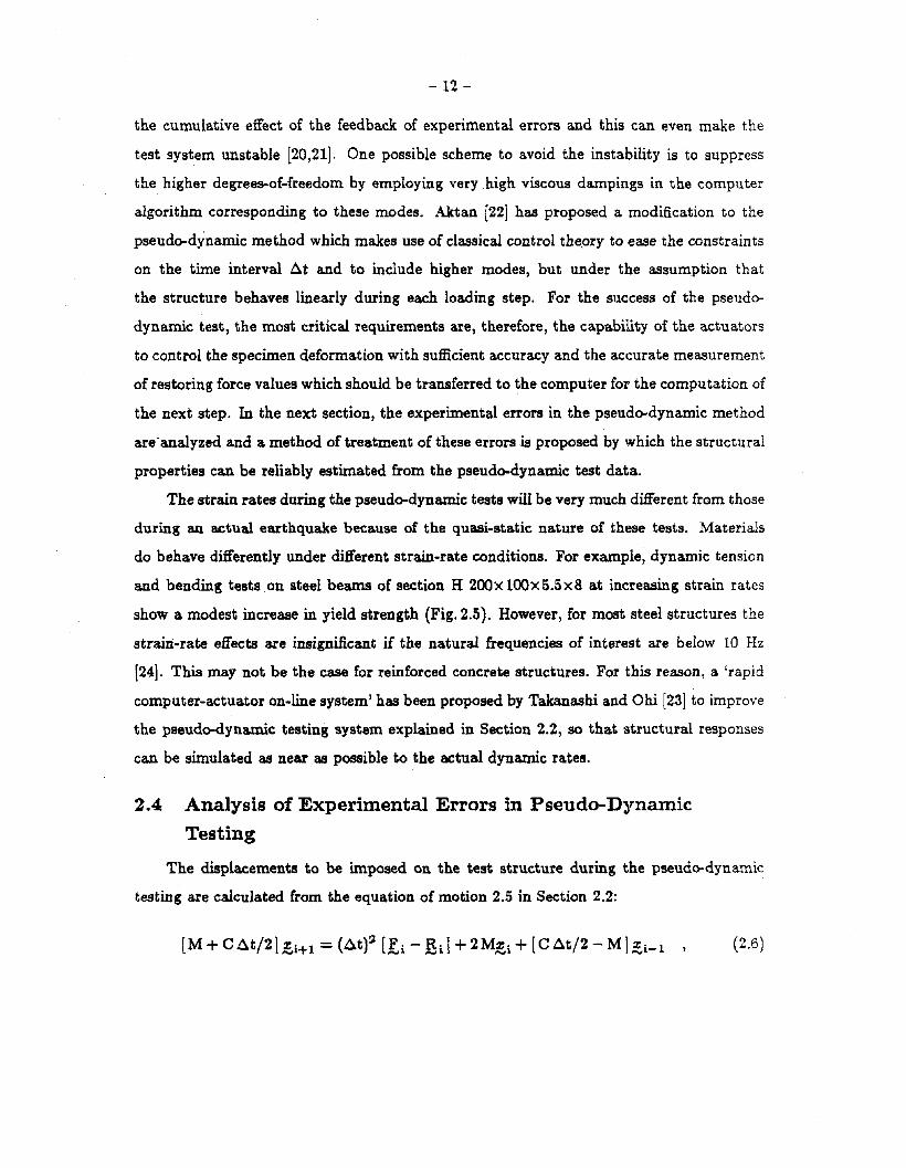
- 12-
the cumulative effect of the feedback of experimental errors and this can even make the
test system unstable [20,21]. One possible scheme to avoid the instability is to suppress
the higher degrees-oi-freedom by employing very high viscous dampings in the computer
algorithm corresponding to these modes. Aktan [22J has proposed a modification to the
pseudo-dynamic method which makes use of classical control the.ory to ease the constraints
on the time interval .6.t and to include higher modes, but under the assumption that
the structure behaves linearly during each loading step. For the success of the pseudo
dynamic test, the most critical requirements are, therefore, the capability of the actuators
to control the specimen deformation with sufficient accuracy and the accurate measurement
of restoring force values which should be transferred to the computer for the computation of
the next step. In the next section, the experimental errors in the pseudo-dynamic method
are'analyzed and a method of treatment of these errors is proposed by which the structural
properties can be reliably estimated from the pseudo-dynamic test data.
The strain rates during the pseudo-dynamic tests will be very much different from those
during an actual earthquake because of the quasi-static nature of these tests. Materials
do behave differently under different strain-rate conditions. For example, dynamic tension
and bending tests on steel beams of section H 200x lOOxS.Sx8 at increasing strain rates
show a modest increase in yield strength (Fig.2.5). However, for most steel structures the
strain-rate effects are insignificant if the natural frequencies of interest are below 10 Hz
[24J. This may not be the case for reinforced concrete structures. For this reason, a 'rapid
computer-actuator on-line system' has been proposed by Takanashi and Ohi [23J to improve
the pseudo-dynamic testing system explained in Section 2.2, so that structural responses
can be simulated as near as possible to the actual dynamic rates.
2.4 Analysis of Experimental Errors in Pseudo-Dynamic
Testing
The displacements to be imposed on the test structure during the pseudo-dynamic
testing are calculated from the equation of motion 2.5 in Section 2.2:
[M + C .6.t/2] ~i+l = (6.tr~ (Ei - Bd + 2M~i + [C .6.t/2 - M I~i-l (2.6)

where
- 13-
~i-l' ~i = displacements calculated at the' previous time steps i-I and i,
Ei = restoring force measured at time step i,
Ii = exciting force due to ground acceleration at time step i, and
~i+ 1 = displacement to be imposed on the test structure at the next
time step.
However, as discussed in the previous section, it is not possible to control the testing
apparatus precisely so that the exact displacements calculated from Eq. 2.6 can be imposed
on the test structure.
Let the displacement-control errors and force-measurement errors at time step i be ~ic
and Eim , respectively; then the restoring forces measured in the elastic tests will be:
(2.7)
where K is the stiffness matrix corresponding to the elastic behavior of the test structure.
Also, if ~im is the displacement-measurement error at the i-th time step, then the
measured displacement £i will be:
(2.8)
(2.9)
where ~i is the displacement calculated from Eq.2.6. Figure 2.6 summarizes the experi
mental errors and shows the feedback of these errors in a flow diagram.
Substitution of Eq. 2.7 in Eq. 2.6 gives:
[M+ C~t/2]~i+l= (~t)2 Ii + [2M - (~t)2K]~i
+ [C ~t/2 - M] ~i-l - (~t)2 [KtiC + Eim1If the cumulative displacement error at time step i is ~i, then the calculated displacement
~i can be written as:
(2.10)
where ~i is the ideal displacement in the absence of experimental errors which satisfies the
following equation:
Subtraction of Eq.2.11 from Eq.2.9 and the use of Eq.2.10 lead to:
[M+C~t/2]~i+l=(~t)2 [-K~iC - Biml + [2M- (~t)2KL~i
+ [C t:"t/2 - M] ~i-l
(2.11)
(2.12)

-14 -
Comparing Eq. 2.12 with Eq. 2.11, it is evident that the cumulative displacement error
~e (t) is the reslJonse of the linear structure to an equivalent exciting force [ - K~ec (t) -
Bern(t) J.
2.4.1 Modal Analysis of Experimental Errors
If the damping matrix C used in the computer algorithm is symmetric and 'classical,'
then the modal column matrix ~, whose columns are the modeshapes of the structure,
. satisfies the following orthogonality relationships:
~TM~ =I, (2.13)
Premultiplication of Eq. 2.12 by the modal row matrix CJ>T gives:
[ ~TM + ~T C 6t/2] xl! = (6t)2 [_~TK xl!C _ ~T R~D11.....1+1 .....1 ..... 1
+ [2 ~T M - (6t)2 CJ>TK1.!i + [~T C6t/2 - ~TMl ~i-l(2.14)
Furthermore, the cumulative displacement error, the displacement-control and force.
measurement errors may be modally decomposed in the following manner:
(2.15)
where e, '1 and f are the modal coordinates, respectively........... ,..,.Substituting Eq.2.15 into Eq.2.14 and using Eq.2.13 gives:
or in component form:
(1 + 6t s"rwr) el~l = (2 - (6twrr~) e~r) + (~t s"r Wr - 1) el~l
- (~t)2 (w; ,,1r) + fi(r»
(2.16)

-15 -
Equation 2.16 can also be written as:
dr) _ ..;.(r) dr) + ..;.(r) c(r) _ (r)~i+1 Y'1 ~i Y'2 ~i-l - ai
where..;.(r) _ 2 - (~twrrzY'l - ,
1 + ~t~rwr
(2.17)
and
where a(r) = (~twr)21 + ~t~rwr
and
The transient and steady-state response statistics of the difference equation 2.17 are ob
tained by the method of operational calculus in Appendix A, in which the steady-state
response variance for the cumulative error (Eq. A.25) is shown to be:
2 ~t
t1(~} = ~r [4 - (~twr)21(2.18)
Equation 2.18 shows that the control errors have a greater effect in the higher modes
whereas the response of the lower modes is affected more by the measurement errors,
provided t1~ and t1J are of the same order for different modes.
2.5 BRI Testing Program
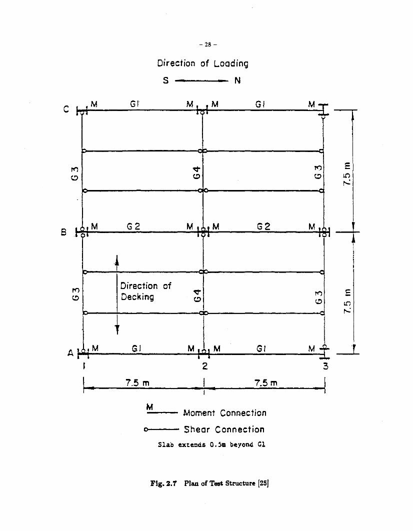
A six-story, two-bay, full-scale steel structure (Figs. 2.7 and 2.8) was tested by the
pseudo-dynamic method at the Building Research Institute (BRI) in Tsukuba, Japan during
November, 1983-March, 1984. This structure, which represented Phase II of the steel pro
gram under the U.S.-Japan Cooperative Earthquake Research Program Utilizing Large
Scale Testing Facilities, was designed to satisfy the requirements of both the 1979 Uniform
Building Code (UBC) of the U.S. and the 1981 Architectural Institute of Japan code, using
eccentric K-bracings [25J. It was 15 mx15 m in plan and 21.5 m high. The two exterior
frames A and C are unbraced moment-resisting frames with one column in each oriented
for weak-axis bending in order to increase the torsional stiffness, and the interior frame
B is a braced moment-resisting frame with eccentric K-bracing in its north bay. All the
girder-to-column connections have been designed as moment connections in the loading

- 16-
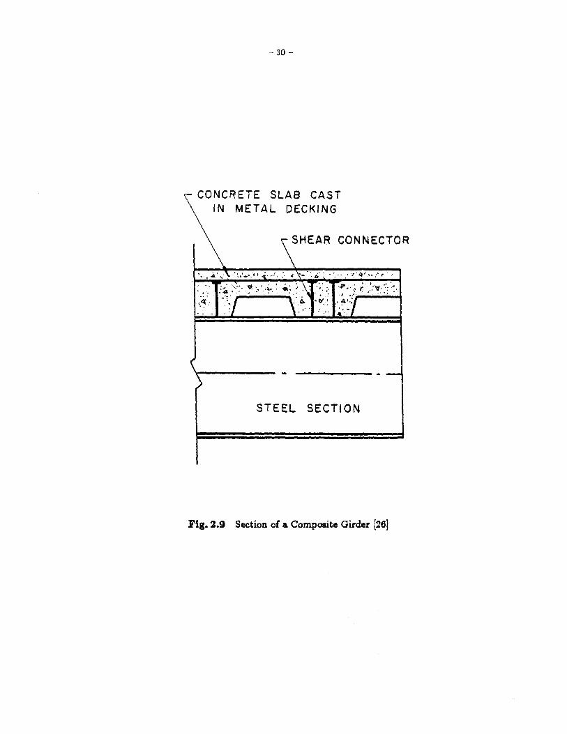
direction and shear connections in the transverse direction. The floor system consisted of a
formed metal decking with cast-in-place light-weight concrete acting compositely with the
girders and floor beams (Figs. 2.9 and 2.10). No non-structural component was attached
to the frame system.
The eccentric-braced frame is a new type of str~ctural system for ea.rthqua.ke resistant
design [271 which has a high elastic lateral stiffness as in concentric braced frames but in
addition has a good energy dissipation capacity due to active shear links, whereas concentric
braces can buckle under compressive cyclic loading and so suffer a drastic decrease in their
buckling strength and their ability to dissipate energy.
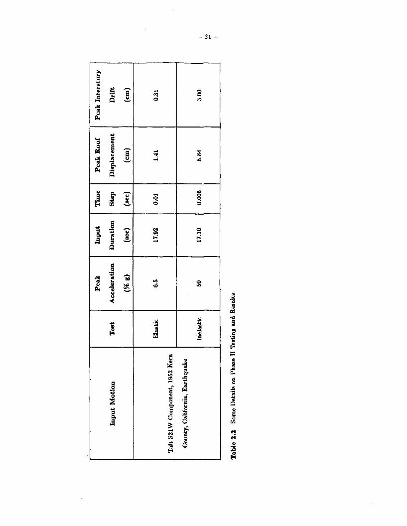
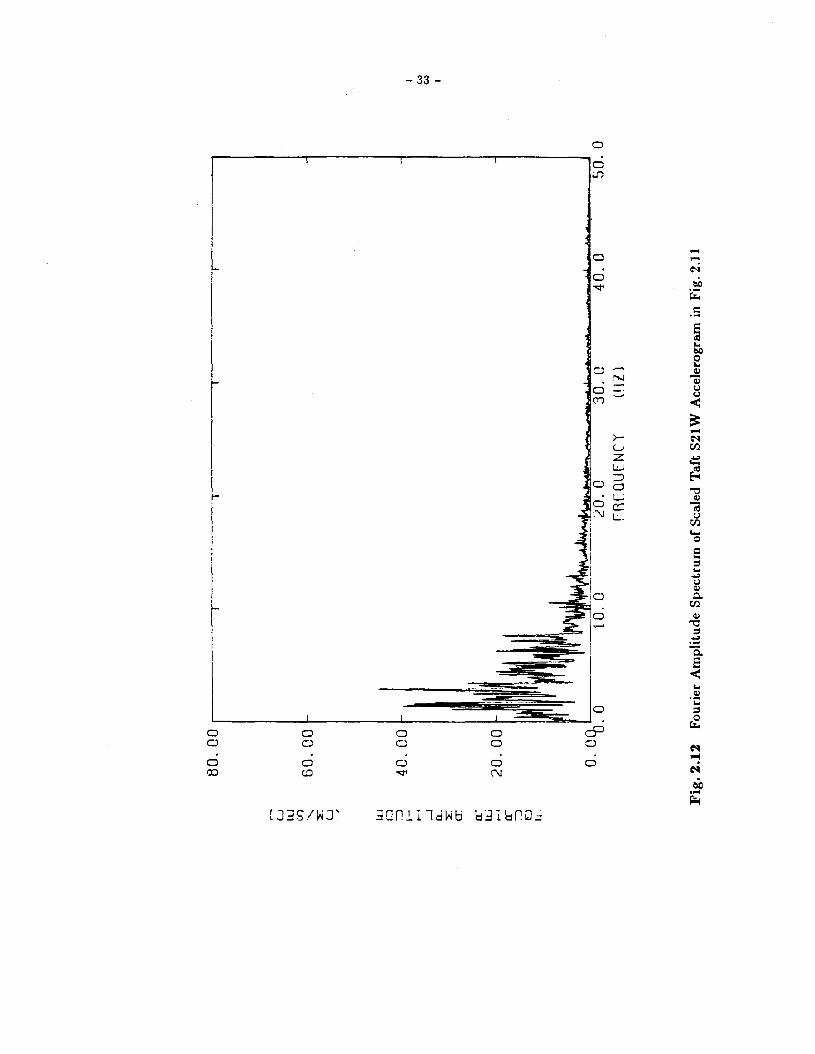
The BRI tests were performed at low amplitudes to give nominally elastic response and
at larger amplitudes to excite the structure into the inelastic range. The uni-directional
loading in the elastic and inelastic tests was produced by an early digitized version (not
the Caltech Vol. nAOO4 version) of the Taft S21W component from the 1952 Kern County,
California, earthquake (Fig. 2.11) scaled to peak accelerations of 6.5% g and 50% g, respec
tively. The Fourier amplitude spectrum of the ground accelerations is shown in Fig. 2.12
[281.During the inelastic test, yielding in shear links, brace gusset plates and some columns
was observed. Overall, the structure performed very well without much visible damage, so
additional three large-amplitude tests were performed using sinusoidal ground accelera.tion
pulses of one cycle each in order to explore the ultimate strength, ductility a.nd failure
mechanism of the structure [29}. Table 2.2 summarizes some of the elastic and inelastic
test details.
- 17-
REFERENCES
[1] Beck, J.L., "Determining Models of Structures from Earthquake Records," ReportNo. EERL 78-01, Earthquake Engineering Research Laboratory, California Instituteof Technology, Pasadena, California, June, 1978.
[2] Charney, F.A. and Bertero, V.V., "An Evaluation of the Design and Analytical SeismicResponse of a Seven-Story Reinforced Concrete Frame-Wall Structure," Report No.UCB/EERC-82/08, Earthquake Engineering Research Center, University of California, Berkeley, California, 1982.
[3] Chavez, J.W., "Study of the Seismic Behavior of Two-Dimensional Frame Buildings:A Computer Program for the Dynamic Analysis-INDRA," Bulletin of the International Institute of Seismology & Earthquake Engineering, Vol. 18, Building ResearchInstitute, Tsukuba, Japan, 1980.
[4] Bertero, V.V. and Moazzami, S., "U.S.-Japan Cooperative Earthquake ResearchProgram: General Implications of Research Results for the 7-Story Reinforced Concrete Test Structure on the State of U.S. Practice in Earthquake Resistant Design ofFrame-Wall Structural Systems, " Proceedings of the 6th Joint Technical CoordinatingCommittee Meeting, U.S.-Japan Cooperative Research Program Utilizing Large-ScaleTesting Facilities, Maui, Hawaii, June, 1985.
[5] Boutros, M.K. and Goel, S.C., "Pre-Test Analysis of the Six-Story Eccentric BracedSteel Test Building," Proceedings of the 5th Joint Technical Coordinating CommitteeMeeting, U.S.-Japan Cooperative Research Program Utilizing Large-Scale TestingFacilities, Tsukuba, Japan, February, 1984.
[6] Goel, S.C. and Boutros, M.K., "Analytical Study of the Response of an EccentricallyBraced Steel Structure," Proceedings of the ASCE Structural Engineering Congress'85, Chicago, illinois, September, 1985.
[7] Wallace, B.J. and Krawinkler, H., "SmaIl-Scale Model Experimentation on Steel Assemblies: U.S.-Japan Research Program," Report No. 75, The John A. Blume Earthquake Engineering Center, Department of Civil Engineering, Stanford University, Stanford, California, June, 1985.
[8] Bertero, V. et al., "Earthquake Simulator Tests and Associated Experimental, Analytical and Correlation Studies of One-Fifth Scale Model, " Earthquake Effects onReinforced Concrete Structures: U.S. -Japan Research, Wight, J .K. (ed.), AmericanConcrete Institute, Detroit, Michigan, 375-424, 1985.
[9] Clough, R.W. and Bertero, V.V., "Laboratory Model Testing for Earthquake Loading," Journal of the Engineering Mechanics Divi8ion, ASCE, Vol. 103(6), 1105-1124,December, 1977.
[10] Beck, J.L., "System Identification Analysis Applied to Full Scale Test Data," Earth·quake Research AjJiiates Conference, California Institute of Technology, Pasadena,California, February, 1985.
[11] Takanashi, K. et al., "Non-Linear Earthquake Response Analysis of Structures by

- 18-
a Computer-Actuator On-Line System," Bulletin of Earthquake Resistant StructureResearch Center, No.8, Institute of Industrial Science, University of Tokyo, Japan,1-17, December, 1974.
[12] Takanashi, K., Udagawa, K. and Tanaka, H., "A Simulation of Earthquake Response ofSteel Buildings," Proceedings of the 8th World Conference on Earthquake Engineering,New Delhi, India, 3156-3162, January, 1977.
[13] Takanashi, K., Udagawa, K. and Tanaka, H., "Earthquake Response Analysis of aI-Bay 2-Story Steel Frame by Computer-Actuator On-Line System," Bulletin of Earthquake Resistant Structure Research Center, No. 11, Institute of Industrial Science,University of Tokyo, Japan, 55-60, December, 1977.
[14] Takanashi, K., Udagawa, K. and Tanaka, H., "Pseudo-Dynamic Tests on a 2-StorySteel Frame by Computer-Load Test Apparatus Hybrid System," Proceedings of the 7thWorld Conference on Earthquake Engineering, Istanbul, Turkey, 225-232, September,1980.
[15] 'Takanashi, K. and Taniguchi, H., "Pseudo-Dynamic Tests on Frames Including HighStrength Bolted Connections," Proceedings of the 7th World Conference on EarthquakeEngineering, Istanbul, Turkey, 445-448, September, 1980.
[16] Okamoto, S. et al., "Techniques for Large Scale Testing at BRI Large Scale StructureTest Laboratory," Research Paper No. 101, Building Research Institute, Ministry ofConstruction, Japan, May, 1983.
[17] Shing, P.B. and Mahin, S.A., "Experimental Error Propagation in PseudodynamicTesting," Report No. UCB/EERC-83/12, Earthquake Engineering Research Center,University of California, Berkeley, California, June, 1983.
[18] Mahin, S.A. and Shing, P.B., "Pseudodynamic Method for Seismic Testing," Journalof Structural Engineering, ASCE, Vol. 111(7), 1482-1503, July, 1985.
[19] B.R.I. Steel Group, "Inelastic Behavior of the Structural Members in the Phase I Test,"Proceedings of the 8th Joint Technical Coordinating Committee Meeting, U.S.-JapanCooperative Research Program Utilizing Large-Scale Testing Facilities, Maui, Hawaii,June, 1985.
[20J Kaminosono, T. et al., "Trial Tests on Full Scale Six Story Steel Structure," Proceedings of the -lth Joint Technical Coordinating Committee Meeting, U.S.-Japan Cooperative Research Program Utilizing Large-Scale Testing Facilities, Tsukuba, Japan,June, 1983.
[21] Yamazaki, Y., Nakashima, M. and Kamin08ono, T., "Note on High Frequency Error inMDOF Pseudo Dynamic Testing," Proceedings of the -lth Joint Technical CoordinatingCommittee Meeting, U.S.-Japan Cooperative Research Program Utilizing Large-ScaleTesting Facilities, Tsukuba, Japan, June, 1983.
[22J Aktan, H.M., "Pseudo-Dynamic Testing of Structures," Journal of Engineering Mechanics, Vol. 112(2), 183-197, February, 1986.
[23] Takanashi, K. and Ohi, K., "Earthquake Response Analysis of Steel Structures by

- 19-
Rapid Computer-Actuator On-Line System," Bulletin of Earthquake Resistant Structure Research Center, No. 16, Institute of Industrial Science, University of Tokyo,Japan, 103-109, March, 1983.
[24] Shing, P.B. and Mahin, S.A., "Pseudodynamic Test Method for Seismic PerformanceEvaluation: Theory and Implementation," Report No. UCBjEERC-84jOl, Earthquake Engineering Research Center, University of California, Berkeley, California,January, 1984.
[25] Askar, G., Lee, S.J. and Lu, L.-W., "Design Studies of the Six Story Steel Test Building:U.S.-Japan Cooperative Earthquake Research Program," Report No. 467.3, FritzEngineering Laboratory, Lehigh University, Bethlehem, Pennsylvania, June, 1983.
[26] Rides, J.M. and Popov, E.P., "Cyclic Behavior of Composite Floor Systems in Eccentrically Braced Frames," Proceedings of the 6th Joint Technical Coordinating Committee Meeting, U.S.-Japan Cooperative Research Program Utilizing Large-Scale TestingFacilities, Maui, Hawaii, June, 1985.
[27] Roeder, C.W. and Popov, E.P., "Eccentrically Braced Steel Frames for Earthquakes,"Journal of th.e Structural Division, ASeE, Vol. 104(3), 391-412, March, 1978.
[28] Hall, J.F ., "An FFT Algorithm for Structural Dynamics," Earthquake Engineering andStructural Dynamics, Vol. 10, 797-811, 1982.
[29J Goel, S.C. and Foutch, D.A., "Preliminary Studies and Test Results of EccentricallyBraced Full-Size Steel Structure," Proceedings of the 16th Joint Meeting, U.S.-JapanPanel on Wind and Seismic Effects, National Bureau of Standards, Washington, D.C.,May, 1984.

- 20-
Type Excitation Amplitudes Scale Cost/Time Comments
Ambient Microtremors, Wind, LimitedSmall Full Cheap/Short
Vibrations Cultural Noise Information
Building Harmonic Small- Not a.t Earth-Full Cheap/Short
Shaker force medium quake Levels
Validity of
Shaking Earthquake Expensive/ Scaling,Large Reduced
Table Record Long Structure/Table
Interact ion
Inertia ModelingPseudo- Evthquake Expensive/
Large Full Errors,Dynamic Record Long
Unstable Control
Extensive
FullCheap/
Natural Earthquake Large InstrumentationUnscheduled
not Practical
Table 2.1 Testing Siruciureslor Earthquake Dynamics [10/
Pea
kIn
pu
tT
ime
Peak
Ro
of
Pea
kIn
ters
tory
Inp
ut
Mo
tio
nT
est
Acc
eler
atio
nD
ura
tio
nS
tep
Dis
pla
cem
ent
Dri
ft
(%g)
(sec
)(s
ec)
(em
)(e
m)
Ela
stic
6.5
17.9
20.
011.
410.
31
Taf
t82
1W
Com
pone
nt,
1952
Ker
n
Cou
nty,
Cal
ifor
nia,
Ear
thqu
ake
Inel
asti
c50
17.1
00.
005
8.84
3.00
Tab
le2
.2S
ome
Det
ails
onP
hase
IIT
esti
ngan
dR
esul
ts
I t,;) ....

- 22-
ROOF
INTERSTORY
SYSTEM BEINGMODELLED
... .z( t )
Fig.2.1 A Multi-Story Building Structure Excited by Ground Accelerations

25.5
m
DISP
LACE
K:NT
TRAN
SDUC
ER\
REAC
TION
WALL
ITV
CAl'E
RA
c¢J1
~.~
HYDR
AULI
C
HYDR
AULI
CPO
WER~
CONT
ROL
PANE
LSU
PPLY
PIlN
ITO
RS.
VIDE
OS&
DISP
LAYS
I
COIt'U
TER
FOR
SERV
OCO
NTRO
LSE
RVO
CONT
ROLL
ERS
STAT
ICDA
TAAC
QUIS
ITIO
NUN
Il
I N "" I
DYNA
/,,\I(
DATA
Am
lJlS
ITIO
fllf
llT
Fig
.2.2
Pse
udo-
Dyn
amic
Tes
ting
Fac
ilit
yat
the
Bui
ldin
gR
esea
rch
Inst
itu
tein
Tsu
ku
ba,
Jap
an[1
6]

- 24-
'i (t) [\
- 'V t
-
Input Ground Accelerations
I
Numerical Solution of Equation
of Motion of the Test Structure
for Displacements ~i+l at Step i + 1
Impose Displacements ~i+l on the
Structure using Hydraulic Actuators
Measure Restoring Forces Ei+l
from the Structure using Load Cells
.,Set i =i+ 1
Fig.2.3 A Simplified Flow Diagram for Pseudo-Dynamic Test Operation [17]

- 25-
0.05Eu
E><Iu
><f-ZI.&J~I.&JU<t 0.00-Ia.en-0a:0a:a:::I.&J
6 - STORY
0.40.0- 0.05 ~----..,.-.----":""'-----------l
-0.4
I NCREMENT OF DISPLACEMENT ~Xe I em
Fig. 2.4. A Typical Plot Showing Displacement Errors During Pseudo-Dynamic Testing[191

1.2 I-
t/)t/)O~..Ja::1.LI~t/)>-
OU..JI.LI~_4>-1-
t/)
I
t/)
ct;:)
o
- 26
1.4 ,------r--.-----"r-------1r------...,DAVIES a NEAL~(after Manjoine) ,
6 ~
• .6 ,," _~ ,,,,,,0 ... .,,'
~---~~---- .10·-0- ti1 F 0 -• TENSION TEST { LANGE
WEB •
BENDING TEST{ FLANGE 6WEB •
0.8 '-- .J.I~----~I----..I.I------.J
10 102 103 104 I o~
STRAIN RATE, jJ./sec
Fig.2.5 Increase of Yield Stress due to Strain Rate [23]

- 27-
Compute Displacement ~I
from Eq.2.6
Impose £1:
z' = z· + zl!c....,1 ....,1 ....,1
R'· = R(%'.),."., 1 ,...,,..,,1
~
Measurements:
zTf1 = z'. + zf!1D1"'lW'1 .-...,,1 ,..",,1
R. = R'. + Rf!1D,.."" 1 ,ow 1 ,..., 1
Set i =i+ 1
Fig.2.6 Feedback of Experimental Errors in Pseudo-Dynamic Testing
- 28-
Direction of Loading
5 - • N
E
MGIMMGIMt , , f -...r ~ I '. -,.~ -
V T'C?C) 0
- -
• c"M G2 M, ." M G2 M• ,• )' I H r :fl
,~ ---Direction ofDecking ~ r<")
C) <-'-- -
t, I",M Gl M 11~. M Gl MJ~• & r I _...A
c
8
• 7.5 m
2
• I • 7.5 m•
MMoment Connection
000--- Shear Connection
Slab extends O.5m beyond Gl
Fig. 2.T Plan of Test Structure [25]

I "-J
(0 I
Be
$N
4.5
m
-l17
m
5@
30
4m
)
- ( -
,~
m,"
,'"
"~
r--7
.5m-+
-7.5
m--t
3 2R 5 46
23
23
Ext
eri
or
Fra
mes
Aan
dC
Inte
rio
rF
ram
eB
(Be
=E
cce
ntr
icB
race
;Pha
sen
)
Fig
.2.8
Ele
vati
onV
iew
sof
Ext
erio
ran
dIn
teri
orF
ram
eso
fT
est
Str
uct
ure
1251
- 30-
CONCRETE SLAB CASTIN METAL DECKING
SHEAR CONNECTOR
STEEL SECTION
Fig.2.9 Section of a Composite Girder [261

FE
MA
LEE
ND
OF
LA
P-J
OIN
T
Fig
.2.1
0T
ypic
alM
etal
Dec
king
used
inC
ompo
site
Con
stru
ctio
n[2
6 1
MA
LE
EN
DO
FL
AP
-JO
INT
I ""....

100
.0
0r---------
--T
--
II
-----.-
------
u5
0.0
0w (J
') .......
u w (J')
.......~ u .....
.O
.0
0I.
"~I"
"'I
IlU
I1.1
1V
III1
1I1
11
1'.1
1'1
11
11
18
11
III
IIII
IIII
IDII
YI
1111
1111
1111
1111
11II
VI1
11
1I1
1I
Id
UIl
III
IIlr
V1\1
1J
11
.11
1I1
11
1-1
11
1"1
I wz
I1
~Ill'
,I
III'1
/~III
'n
'III
WI/II
-IU
1111
'1''l
IJII
y~
~'I
t>:l
EJ
I
.......
I- a: a: w
-50
.00
---.J w U u cr.
-10
0.
0Cb
~0
--t-O-----------8~O-----
12~
016
~0
20
:0
TIM
E(S
EC
)
Fig
.2.1
1T
aft
821
WA
ccel
erog
ram
,19
52K
ern
Co
un
ty,
Cal
ifor
nia,
Ear
thq
uak
e(p
eak
scal
edto
6.5%
g)
80
.00
II
II
II
u w en "-6
0.0
0....
y u w o ::l
1- ...' -l
IL :L a: cr l1.j ..... lr ::l
o U
40
.0
0~
20
.00
I V)
V) I
o.oCb~
o~
10
.-0-
-1,.~
2.0
.0fR
fQU
EN
C,
30
.0(H
l)
40
.05
0.a
Fig
.2.1
2F
ouri
erA
mp
litu
de
Sp
ectr
um
ofSc
aled
Taf
tS2
1W
Acc
eler
ogra
min
Fig
.2.1
1

- 34-
CHAPTER 3
SYSTEM IDENTIFICATION APPLIED TO THE ELASTIC
PSEUDO-DYNAMIC TEST DATA
-IGNORING FEEDBACK OF EXPER.Il\fENTAL ERRORS
3.1 Introduction
In system identification, we are concerned with the determination of system models
from records of system operation [1,10]. The problem can be represented diagrammatically
as Fig. 3.1 in which
).!.(t) =known input
~(t) = system output
~(t) =process noise (e.g., unknown inputs)
.!!.(t) =observation noise
yet) =measured output.....Thus, the problem of system identification is the determination of a system model from
records of u(t) and yet). In other words, given the input-output data set for a real system,.... ....we want to obtain a mathematical model which describes a certain behavior of the system.
We will be concerned with parametric system identification in this study, in which
a particular mathematical form is chosen to describe the essential features of the system
and then the unknown parameters of the model are estimated from the input and output
data. In contrast, in nonparametric system identification, functions rather than parameters
are estimated, such as a transfer function or impulse response function. In practice, only
discrete values of the functions can be estimated and so, in effect, a model with a very large
number of parameters must be estimated. This makes the results very sensitive to model
error and measurement noise. Nonparametric models have been discussed by Beck [2].

- 35-
3.2 Output-Error Method for Parameter Estimation
In this section, the output-error approach to parameter estimation is described, follow
ing Beck [2]. In this method, the parameters of a model are estimated by determining those
values which give an optimal match of the output of the model and the measured output
of the real system, when both are subjected to nominally the same input. The quality of
the output match is determined by some scalar function J of the output-error called the
measure-of-fit. The parameter ·adjustment algorithm shown in Fig.3.2 selects the optima.l
parameter values by minimizing the measure-of-fit J in a systematic manner.
The output-error e is the difference between the output measurements y of the system,." ,."
and the model output m:,."
£,(tj 1J = 1..(t) - m(tj 1J (3.1)
In structural identification, the output vector y will be the recorded response such as,."
displacement, velocity or acceleration at various points in the structure.
For a given observed input z(t) and measured output y over a time interval [ts , t e ],,."
the optimal estimates of the parameters are defined to be the values which minimize the
measure-of-fit:
1t.
J(!) = < £,(tj!) , V,!(t;!) >t.
dt , (3.2)
where < ., . > is the Euclidean scalar product and V is a prescribed positive definite
diagonal matrix which allows weighting of the output-error.
The problem of identifying the optimal model from system data has been now reduced
to minimizing the function J(!) in Eq.3.2. This minimization could be achieved by directly
solving the stationarity condition of J with respect to 1.:
(3.3)
where 9 is the vector of optimal parameter estimates. This usually leads to a set of si-,."
multaneous nonlinear algebraic equations in! which cannot be solved analytically. The
nonlinearity arises because the model response is, in general, a nonlinear function of the
parameters, even if the model itself is linear in the state and linear in the parameters.
Some descent methods for optimization which have been used in structural identifica
tion include the Gauss-Newton method, the method of steepest descent and the conjugate

- 36-
gradient method. The Gauss-Newton method is equivalent to applying to Eq. 3.3 a mod
ification of the classical Newton-Raphson method for finding the zeros of a multi-variable
vector function.
A descent method called the modal minimization method, developed by Beck and
Jennings [3J to provide a reliable technique for the identification of linear modal models, is
used in this study.
3.3 Linear Structural Model
3.3.1 Analytical Model
A discrete analytical model which has the following equation of motion:
Mx + Dx + Kx =- Mz(t) 1 ,/">oJ ""'-I""" ,...,.,
with the initial conditions
and
(3.4)
represents a physical model consisting of a distribution of lumped masses linked by linear,
massless springs and dashpots, with the base being rigid and moving in only one direction.
The vector ~ = [Xl, X2,'" ,XN ]T then consists of horizontal displacement relative to the
base of each degree of freedom of each lumped mass of the model, and z is taken to be
the horizontal component of acceleration of the base motion. All the components of 1 are""
unity. M,D and K are mass, damping and stiffness matrices, respectively, and along with
the initial conditions form the parameters of the model.
With respect to the inverse problem, Beck [2J showed that the stiffness and damping
matrices are not determined uniquely in typical situations. The first limitation arises from
the fact that seismic response is usually measured at only a few points in a structure while
'local' uniqueness of K and D requires measurement of response at !N or more of the
coordinates. Another important limitation is due to the deterioration of the signal-to-noise
ratio at higher frequencies, implying that the higher mode information in the stiffness and
damping matrices will be unreliable if attempts are made to estimate these matrices from
seismic records.
On the other hand, modal parameters for the structure can theoretically be determined
which contain all the information about the structural properties that can be estimated

- 37-
directly from the input and output records, although the small signal-to-noise ratio at
higher frequencies implies that only the dominant modes of the response can be estimated
reliably from earthquake data. Beck [21 then concluded that when linear models are to
be estimated from seismic excitation and response time-histories, they should be based on
the dominant modes in the records of the response and not on. the stiffness and damping
matrices. If estimation of structural parameters is of interest, this may be done in a separate
stage using the identified modal parameters.
3.3.2 Modal Model
If the mass matrix M is assumed symmetric and positive definite, then a real inner.
product in RN can be defined as :
(3.5)
where R N is an N-dimensional Euclidean vector space. Also, the stiffness matrix K a.nd
the damping matrix D being assumed symmetric matrices and K also being assumed a
positive definite matrix [Le., self-adjoint and positive definite operators with respect to the
usual innerproduct ( z, y) = zTYI, it can be shown that M-lK and M-lDare self-,..., """"" "'"'J ,...",
adjoint operators and M-lK is also a positive definite operator, but with respect to the
innerproduct defined in Eq.3.5. Furthermore, if the damping is assumed to be classical,
then M-IK and M-ID are commutative.
The above properties of M-1K and M- l D ensure that they have a common set of N
orthonormal eigenvectors [41 such that:
M-IK~=~n2
M-lD~=~(2Zn)
(3.6)
where c) = [<p(l), <p(2) , "', <p(N) 1 denotes the modeshape matrix whose columns are the,.,.,.,. .....eigenvectors of M-1K and M-1D. Also
[
WOl0= and z= [: ('.]
where the Wr and )r are the modal frequencies and modal damping factors, respectively.

- 38-
Since ~ gives an orthonormal basis for R N with respect to the innerproduct defined
in Eq.3.5,
Premultiplying Eq. 3.6 by ~T and using Eq.3.7:
(3.i)
and (3.8)
Since the eigenvectors fj>(r) are a basis for the N-dimensional space R Nl X can be written,... .....
as:
£(t) = ~ f(t} "1£ ERN
N (3.9)=2: er(t) t(r)
r=l
where eis the vector of coordinates of % with respect to the basis of eigenvectors.,... ,...
Substituting Eq. 3.9 into Eq.3.4:
Premultiplying Eq. 3.10 by "T and using Eqs. 3.7 and 3.8:
e+ 2Zn e+ 02e= -"TMz(t) 1~ ,.." f'o<,J ~
= -2z(t) ,
(3.10)
(3.11)
where () is the vector of modal participation factors whose magnitude in general depends,...
on the normalization used for~, such as Eq.3.7. Hence it is useful to express Eqs. 3.9 and
3.11 in forms which are invariant with respect to any particular normalization introduced
for ~.
Equation 3.9 can also be written as:
where
N
%i(t) = L %~r)(t} )r=1
(3.12)
(3.13)
and is the contribution from the r-th mode to the response at degree-of-freedom i.
From Eqs.3.11 and 3.13, the following equation can be deduced:
(3.14)

- 39-
where p~r) = cP~r) an is called'the effective participation factor for the r-th mode at the i-th
degree-of-freedom, and it is independent of the normalization chosen for the ¢(r) ......The corresponding initial conditions for Eq.3.14 are:
N
x[r) (ta) = ¢[r) Er (ta ) = cP~r) L cP}r) mjk Xk (ta)
j,k=l
N
x~r) (ta) = cP!r) er (ta) = cP~r) 2: cPj(r) mjk Xk (ta)
j, k=l
Summary:
(3.15)
with the initial conditions
andN
Xj(t) =2: x~r)(t) .r=l
(3.16)
Hence the parameters of the modal model to be estimated are:
{ (r) (r) ( ) . (r) (t ) .' - 1 2 N}Wr , )r, Pi , Xi t a , Xi a' I, r - , , ••. , .
3.4 Single-Input Single-Output (SI-SO) System Identification
Technique
A single-input single-output system identification technique may be used to estimate
the modal parameters when the input and output consist only of one component of ground
motion and a parallel component of response at some point in the structure, respectively.
The parameters to be estimated are the modal parameters:
r =1,2,···,R ,
where each modal contribution, x(r) (t), is governed by the standard equation of motion:
with the initial conditions (3.17)

- 40-
Comparing Eqs. 3.16 'and 3.17:
O(r) - w21 - r'
ll(r)172 == 2S'r Wr , O
(r) _ (r)3 - Pi
and R is the number of dominant modes in the structure contributing at the point of
consideration.
Let the measured output history be:
(3.18)
over some time interval [ts , tel, then any combination of displacement, velocity or accelera
tion records of one component of the structural response at a point can be used by choosing
each Ki as either 1 or O.
The corresponding model output is:
(3.19)
where the response at each floor is modelled as a superposition of the contributions of a
small number, R, of classical modes so that:
R
:t(tj £,) =L :t(r) (tj !(r)),,=1
and
From Eq. 3.1, the output-error is:
The measure-of-fit can be obtained by substituting Eq.3.21 into Eq.3.2:
(3.20)
(3.21)
where (3.22)
The diagonal weighting matrix V has been chosen to normalize each integral in Eq. 3.22 in
order to give a meaningful comparison between the optimal values of J for different time

- 41-
segments and for different response quantities. The optimal estimates of the parameters
are obtained by minimizing the above measure-of-fit by the modal minimization method.
This method, which is explained in detail by Beck in his thesis dissertation [2], is given
very briefly in the following section.
3.4.1 Modal MinimizatioD Method
The method consists of three parts:
(a) Modal Sweeps
(b) Single-Mode Minimizations
(c) One-Dimensional Minimizations
(a) Modal Sweeps
Initial estimates are made for 8 = [8(1) ,8(2) " •• ,g(R) ]T. Then the following sequence"""-I """'i""'" ,..""
of minimizations, which is called a modal sweep, is applied:
min= 0(1)-
J (0(1) 0<2) ••• o(R») = min J (i1) 0(2) ••• O(R»)- '- "- 0(2) - '- , '--
J (i1) 0<2) ••• i R») = min J (0<1) 0<2) ... i R- 1) O(R»)_ ,_ "_ g(R) _,_, ,_ ,_-
(3.23)
Each of the above steps involves minimization at the modal level and is called a single-mode
minimization. Successive sweeps are performed until the change in J is insignificant.
(b) Single-Mode MinimizatioDs
The minimization of JCt) in Eq. 3.22 with respect to !(r) is equivalent to minimizing
the function:
(3.24)
whereR
x~r) = Xo - L X(I) ,
."'1;6r
R
v~r) = Vo - L :i:(I) ,
.=1;6r
R
a~r) = ao - L %(1) .
.=1;6r
- 42-
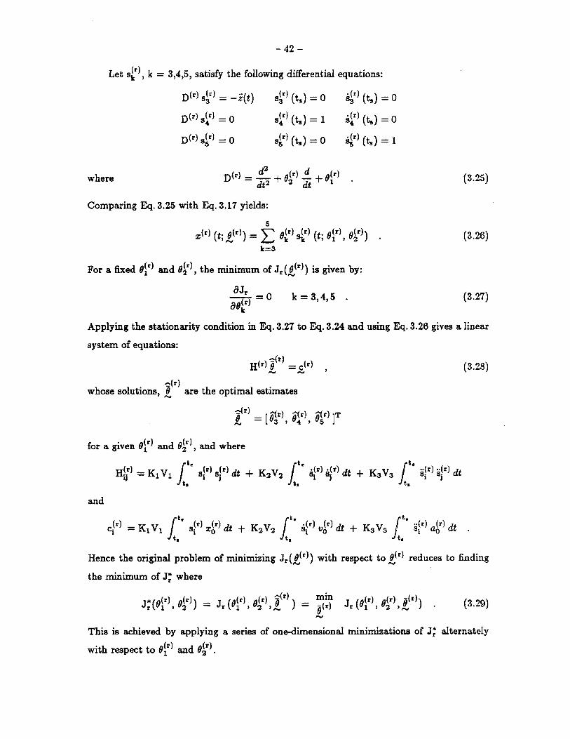
Let s~r), k = 3,4,5, satisfy the following differential equations:
n(r) (r) - "(t)s3 --z
n(r) s~r) = 0
n(r) s~r) = 0
s~r) (ts ) = 0
s~r) (ts ) = 1
s~r) (ts ) = 0
s~r) (ts ) = 0
sir) (ts ) = 0
s~r) (ts ) = 1
where (3.25)
k = 3,4,5 .
Comparing Eq. 3.25 with Eq. 3.17 yields:
5x(r) (t· O(r)) - '" O(r) s(r) (t· O(r) O(r»),_ - L-, It It I 1 , 2
1t=3
For a fixed oir) and o4r), the minimum of Jr(t(r») is given by:
aJr = 0ao(r)
It
(3.26)
(3.27)
Applying the stationarity condition in Eq. 3.27 to Eq. 3.24 and using Eq. 3.26 gives a linear
system of equations:
(3.28)
~(r)
whose solutions, 0 are the optimal estimates"'"
for a given oir) and o4r), and where
and
Hence the original problem of minimizing Jr(i(r)) with respect to !(r) reduces to finding
the minimum of J; where
J*r (O(lr), 02(r») = J (O(r) O(r) j(r)) - mm J (O(r) O(r) g(r))r 1 I 2 I_ - g(r) r 1 I 2 ,_- (3.29)
This is achieved by applying a series of one-dimensional minimizations of J; alternately
with respect to oir) and o4r).

- 43-
(c) One-Dimensional Minimizations
J; is minimized alternately with respect to ell:) and e~l:) as shown in Fig. 3.3. This
process is continued until a consecutive pair of one-dimensional minimizations results in a
fractional decrease in J; of less than a specified tolerance. This technique for minimizing J;with respect to oir
) and O~r) turns out to be equivalent to the method of steepest descent,
after the first step, as seen in Fig. 3.3, but with the advantage that the gradients of J; with
respect to eir) and O~r) need not be computed.
To evaluate J; in Eq.3.29, first the linear differential equations in 3.25 are solved for
the 'sensitivity coefficients' using the transition-matrix method of Nigam and Jennings [5].
This method gives exact solutions at each time step for a linear variation of the ground
accelerations z(t) within each time step. Equation 3.28 is then solved using Gaussian
elimmation for -rr) and the contribution of the r-th mode to the response is calculated,...
from Eq.3.26. The value of J; can then be obtained from Eq. 3.24 using Simpson's rule for
numerical integration.
3.5 A 81-80 Analysis of Pseudo-Dynamic Elastic Test Data
Using the single-input single-output structural identification method explained in the
previous section, the data from the Phase II 'elastic' test at Tsukuba, Japan, described in
Chapter 2, are analyzed. The principal objectives are:
(a) to examine the validity of the pseudo-dynamic method, within the elastic range
of the structure,
(b) to ascertain how well a linear model with classical normal modes is capable of
reproducing the measured response, and
(c) to determine what damping levels were operative during the elastic test.
As explained in Section 2.3, the higher modes in multi-degree-of-freedom systems are
susceptible to becoming unstable due to the cumulative effects of feedback of experimental
errors in the computer control system. This led to artificial suppression during the test of
the higher structural modes beyond the first three. This was done by effectively adding
large viscous damping factors of 90% of critical to the computer model used to calculate
the experimental displacements to be imposed on the structure during the test. However,
the Fourier amplitude spectrum of the Taft record in Fig.2.12 shows that these higher
modes would not be significantly excited by the earthquake accelerations since their natural
frequencies lie above 10 Hz where the ground motions are negligibly small and, in addition,

- 44-
these modes have relatively small participation factors. It should be noted that since only
three modes can be determined from the test data, it is not possible to use these data
for an inverse calculation to compute the stiffness and damping matrices uniquely for a
six-degree-of-freedom model corresponding to the horizontal motions of each floor, unless
a chain model is assumed.
3.5.1 Identification Results: Two-Mode Models
The results of applying the SI-S0 system identification procedure independently to
each of the displacement histories measured at each floor level are given in Table 3.1. In
this application, the model response is computed from a modal model consisting of just the
first two modes. It is seen from Table 3.1 that the period and damping for the fundamental
mode are estimated as 0.553 sec and 1.2% of critical, respectively, and these estimates·
are remarkably consistent from floor to floor. This is again observed for the period of
the second mode, which is estimated as 0.191 sec. However, the damping of the second
mode shows some scatter about a mean value of 2.1% of critical damping. This scatter is
probably due to the fact that the response of a mode is much less sensitive to changes in
damping than to changes in its period, so that the damping is more difficult to estimate
reliably, again confirming the observation made by Beck and Jennings [3]. The above
difficulty is accentuated by a low signal-t~noise ratio when the second mode is estimated
from the displacement records, since this mode makes a relatively small contribution to the
displacement. Overall, the estimates from each floor and the small values of J, in Table
3.1, suggest that the structural displacement is approximated well by two classical modes
of vibration, each giving structural motions in which all the floors move in phase.
The estimates in Table 3.2 are obtained by the application of SI-S0 technique to the
pseud~velocity record at each floor, again using a tw~mode model. The pseud~velocity
is the velocity calculated by the on-line computer (Fig.2.2) using the central difference
method and displacement history. Since the second mode has a relatively stronger signal
in the velocity, the damping can be estimated more reliably in this case. Hence, much less
variation in the damping estimates is observed for the second mode in Table 3.2 compared
with Table 3.1. The estimates for the periods and dampings in Table 3.2 are again consistent
from floor to floor and the values of J are small, showing the validity of an approximation
of the pseud~velocityby two classical modes of vibration.
Comparing Tables 3.1 and 3.2, it is seen that the estimates of the periods from the

- 45-
two sources, measured displacements and pseudo-velocities, are identical, to within the
precision specified in the tables, for both modes. The damping and effective participation
factors for the fundamental mode are also identical, but there are small differences in the
corresponding values for the second mode in Tables 3.1 and 3.2. Since the second-mode
signal is stronger in the pseudo-velocities than in the measured displacements, a signal-to
noise argument suggests that the effective participation factors in Table 3.2 are the more
reliable estimates.
The small values of the measure-of-fit J shown in Tables 3.1 and 3.2 indicate that a
two-mode model is capable of reproducing the test displacement and velocity responses
very well. This is again demonstrated by the time-history comparisons in Figs. 3.4 and
3.5. Figure 3.4 compares the velocities of the test structure and the optimal two-mode
model at the roof, mid-height (floor 4) and floor 2 using the parameters estimated from the
pseudo-velocity records (Table 3.2). The corresponding displacements are also compared
in Fig. 3.5. Note the larger J-value for floor 2 in Table 3.2. This suggests high frequency
components in the pseudo-velocity record at this floor which require a higher mode model
approximation. A three-mode model is now examined.
3.5.2 Identification Results: Three-Mode Models
In this section, the 51-SO system identification method is applied to the pseudo-velocity
and pseudo-acceleration responses independently, using a linear model consisting of three
modes. The results are shown in Tables 3.3 and 3.4, respectively. The estimates for the
first two modes are again consistent from floor to floor and they are essentially the same
as the estimates for the two-mode model in Table 3.2. The estimates of the third-mode
parameters from both' the pseudo-velocity (Table 3.3) and pseudo-acceleration (Table 3.4)
responses are also very nearly identical. The values of measure-of-fit J in Table 3.3 are
smaller than the corresponding values in Table 3.2, where the pseudo-velocity response was
used to estimate the parameters in both cases, as expected.
However, the surprising results in Tables 3.3 and 3.4 are:
(a) the third-mode damping is negative, and
(b) the measure-of-fit J is relatively large for the optimal three-mode model which
would be expected to be capable of giving a very good match of the pseudo
accelerations since the higher modes beyond the first three were suppressed in the
test (Table 3.4).

- 46-
The response time-history comparisons from the test and the optimal three-mode
model obtained from the pseudo-velocity records are shown in Figs. 3.6 and 3.7. The veloc
ities of the test structure and the three-mode model are compared at the roof, mid-height
and fioor 2 in Fig. 3.6 and the corresponding displacement comparisons are given in Fig. 3.7.
The roof pseudo-acceleration from the test and that calculated from the three-mode model
identified from the roof pseudo-acceleration record are plotted in Fig. 3.8 for successive six
second segments at a larger time scale so that the nature of the high-frequency differences
is easier to observe.
An examination of the Fourier amplitude spectrum of the roof pseudo-acceleration
record (Fig. 3.9) shows that the 'third-mode' signal near a frequency of 10 Hz is much too
large relative to the first- and second-mode signals. This anomaly is also demonstrated
in Fig. 3.10 where the Fourier amplitude spectra for the roof pseudo-accelerations and the
accelerations of the three-mode model identified from the pseudo-acceleration record at the
roof are compared. Both spectra agree very well over a frequency range of the first two
modes, but the third mode from the system identification procedure underestimates the
apparent resonant amplitude from the test, despite the fact that the system identification
procedure has tried to make the third-mode response of the model larger by selecting a
negative damping.
It is concluded that this strong signal around 10 Hz is not entirely due to the excitation
of the third mode by the Taft acceleration record but is partly due to the cumulative effect
of feedback of control and measurement errors during the test, as discussed in Chapter 2.
This unstable growth in the third mode produced the apparent negative damping when
the system identification procedure tried to account for the strong signal solely from the
earthquake excitation.
The equation of motion used to control the test structure is:
Mx + Cz + R(x) = -Mz(t) 1 ,f"'V ~,...,,..., ~
(3.30)
where C represents the nominal damping used in the on-line computer algorithm. But
the linear model used in the system identification procedure can be represented by the
equation:
Mx+ Dz+ Kx = -Mz(t) 1 .,.."" ,.,.",,.,.,,, ",..."
(3.31)
If the cumulative effect of feedback of the measurement and control enors in the pseudo-

- 47-
dynamic test is approximated by an equivalent viscous damping, then D in Eq. 3.31 repre
sents the total viscous damping which is the sum of the viscous damping from the computer
algorithm (e), the structural damping due to some hysteretic action and the apparent
damping due to feedback of experimental errors.
From Table 3.5, the algorithmic dampings used in the pseudo-dynamic test for the
first three modes are 0.35%, 0.35% and 2.00%, respectively. Hence, a negative damping
of -0.05% for the third mode from the linear model of the system identification method
suggests that the experimental errors introduced an equivalent negative viscous damping
in the third mode which is greater than 2% in magnitude. This phenomenon of adding
energy into the third mode explains why the third-mode signal appears very strong in the
Fourier amplitude spectrum in Fig. 3.9.
3.5.3 CODclusioDs
(a) For similar amplitudes to those in the elastic test (peak relative acceleration and
displacement of 30% g and 1.4 cm respectively at the roof), a linear model based on just
two classical modes should give an excellent approximation to the real dynamic. response
of the structure.
(b) At these amplitude levels, the overall equivalent viscous damping factors for the
first two modes are 1.2% and 2.1% of critical. The damping of the fundamental mode is
consistent with the value of 1.25% reported for a pseudo-dynamic free-vibration test per
formed after the elastic test [8]. Part of the damping was artificially introduced as numerical
viscous damping in the computer model used to produce the experimental displacements
(Table 3.5). The cumulative effect of feedback of control and measurement errors also
contributed some damping.
Assuming the latter damping is small for the lower modes, especially the first two
modes, the energy dissipated by the structure itself produced equivalent viscous damping
factors of about 0.9% and 1.8%, respectively, for the first and second modes. These low
values of damping, compared with the values of 3% to 8% from the earthquake response of
tall buildings in the field [9], are most likely due to the absence of both energy dissipation by
nonstructural components and by radiation damping, the latter because of the quasi-static
nature of the test.
(c) The feedback of control and measurement errors into the computer model used
to produce the experimental displacements in the elastic test produced a cumulative error

- 48-
of large amplitude in the pseudo-acceleration at the frequency of the third mode. This
addition of energy into the test structure is further demonstrated by an equivalent negative
viscous damping of at least 2% estimated for the feedback effect in the third mode. However,
these errors have an insignificant effect on the displacements and pseudo-velocities, where
the high-frequency content is greatly reduced. Chapter 4 deals with the estimation of the
actual structural damping and the effect of the experimental errors on the response of the
test structure.

- 49-
REFERENCES
[IJ Sinha, N.K. and Kuszta, B., Modeling and Identification of Dynamic Systems, VanNostrand Reinhold Company Inc., New York, 1983.
[2J Beck, J.L., "Determining Models of Structures from Earthquake Records," ReportNo. EERL 78-01, Earthquake Engineering Research La.boratory, California Instituteof Technology, Pasadena, California, June, 1978.
[3J Beck, J.L. and Jennings, P.C., "Structural Identification Using Linear Models andEarthquake Records," Earthquake Engineering and Structural Dynamics, Vol. 8, 145160,1980.
[4J Lectures by Professor J .L. Beck on Engineering Mathematical Principles, CaliforniaInstitute of Technology, Pasadena, California, 1983-84.
[5] Nigam, N.C. and Jennings, P.C., "Calculation of Response Spectra from Strong-MotionEarthquake Records," Bulletin of Seismological Society of America, Vol. 59,909-922,1969.
(6] Beck, J.L. and Jayakumar, P., "Analysis of Elastic Pseudo-Dynamic Test Data froma Full-Scale Steel Structure Using System Identification," Proceedings of the 6th JointTechnical Coordinating Committee Meeting, U.S.-Japan Cooperative Research Program Utilizing Large-Scale Testing Facilities, Maui, Hawaii, June, 1985.
[7] Beck, J.L. and Jayakumar, P., "Application of System Identification to PseudoDynamic Test Data from a Full-Scale Six-Story Steel Structure," Proceedings of theInternational Conference on Vibration Problems in Engineering, Xian, China, June,1986.
[8J Midorikawa, M., et aI., "Preliminary Test in Phase II," Proceedings of the 5th JointTechnical Coordinating Committee Meeting, U.S.-Japan Cooperative Research Program Utilizing Large-Scale Testing Facilities, Tsukuba, Japan, February, 1984.
[9] Beck, J.L., "System Identification Applied to Strong Motion Records from Structures,"Earthquake Ground Motion and Its Effects on Structures, S.K. Datta (ed.), ASME,AMD-Vol. 53, New York, 1982.
[10] Eykhoff, P., System Identification, John Wiley & Sons, New York, 1977.

- 50-
Mode 1 Mode :I
Effective Effective JFloor
Period Damping Participation Period Damping Participation (%)
. (sec) (%) Factor (Bee) (%) Factor
Roof 0.553 1.2 1.39 0.191 2.3 -0.57 1.2
6 0.553 1.2 1.22 0.191 2.6 -0.25 0.57
5 0.553 1.2 1.00 0.192 1.6 0.13 0.51
4 0.553 1.2 0.77 0.191 1.9 0.39 0.35
3 0.553 1.2 0.53 0.191 2.0 0.47 0.48
2 0.553 1.2 0.30 0.191 2.1 0.37 1.3
Table 3.1 Modal Parameters Eatimated from the Measured Displacement Records Using aTwo-Mode Model and the SI·SO Technique [6J
Model Mode 2
Effective Effective JFloor
Period Damping Participation Period Damping Participation (%)
(sec) (%) Factor (sec) (%) Factor
Roof 0.553 1.2 1.39 0.191 2.2 ·0.53 1.3
6 0.553 1.2 1.22 0.191 2.2 ·0.21 0.34
5 0.553 .1.2 1.00 0.191 2.0 0.16 2.8
4 0.553 1.2 0.77 0.191 2.1 0.42 0.93
3 0.553 1.2 0.53 0.191 2.1 0.48 4.3
2 0.553 1.2 0.30 0.191 2.1 0.36 18.7
Table 3.2 Modal Parameters Eatimated from the Pseudo-Velocity Records Using a Two-ModeModel and the SI·SO Technique [61

- 51-
Mode 1 Mode 2 Mode 3
Floor T f 13 T f 13 T f 13 J
(sec) (%) (sec) (%) (sec) (%) (%)
Roof 0.553 1.2 1.39 0.191 2.2 ..Q.53 0.106 -0.05 0.03 0.75
6 0.553 1.2 1.22 0.191 2.2 -0.21 0.106 -0.04 ..Q.01 0.24
5 0.553 1.2 1.00 0.191 2.0 0.16 0.106 -0.05 -0.05 1.4
4 0.553 1.2 0.77 0.191 2.1 0.42 0.106 -0.06 -0.02 0.62
3 0.553 1.2 0.53 0.191 2.1 0.47 0.106 -0.05 0.02 2.4
2 0.553 1.2 0.30 0.191 2.1 0.36 0.106 -0.05 0.04 9.5
Table 3.3 Modal Parameters Estimated from the Pseudo-Velocity Records Using a Three-ModeModel and the SI-S0 Technique [71
Mode 1 Mode 2 Mode 3...
? ... T ... ... ...?Floor T p ~ p T P J
(see) (%) (see) (%) (sec) (%) (%)
Roof 0.553 1.2 1.39 0.191 2.2 ..Q.53 0.106 -0.05 0.03 11.2
6 0.553 1.2 1.23 0.191 2.2 ..Q.21 0.106 -0.03 -0.01 5.0
5 0.553 1.3 1.01 0.191 2.2 0.17 0.106 -0.05 -0.04 21.0
4 0.553 1.3 0.78 0.191 2.1 0.43 0.106 -0.05 -0.02 8.0
3 0.553 1.2 0.53 0.191 2.1 0.48 0.106 -0.04 0.02 19.6
2 0.553 1.2 0.30 0.191 2.1 0.36 0.106 -0.05 0.04 35.8
Table 3.' Modal Parameters Estimated from the Pseudo-Acceleration Records Using aThree-Mode Model and the SI-S0 Technique [71

- 52-
Critical Damping Ratio (%)
Test Mocl. Comments
1 2 3 4 5 6
Preliminary Free
and Forced 0.354 0.311 - - - - Calculated from Test Response
VibratioD Tests
Elastic Selection Based on Vibration
Pseudo-Dynamic 0.35 0.35 2.00 90.0 90.0 90.0 Test Values and Stability
Test ConsideratioDs
Table 3.5 Damping Values for Tests in Phase II [8]

u ( t )~
- 53-
w t t )~
SYSTEMz( t )~
n ( t )~
y ( t )~
Fig.3.1 Block Diagram nIustrating the System Identification Method [1]

NP
UT
\S
YS
TE
M
MO
DE
L(P
AR
AM
ET
ER
S8
)rv
y rv
m ......
+O
UT
PU
TF
RR
OR
e ......
I en "'"" I
PA
RA
ME
TE
RA
DJ
US
TM
EN
TA
LG
OR
ITH
M
Fig
.3.2
Blo
ckD
iagr
amIl
lust
rati
ngth
eO
utp
ut-
Err
or
Met
hod
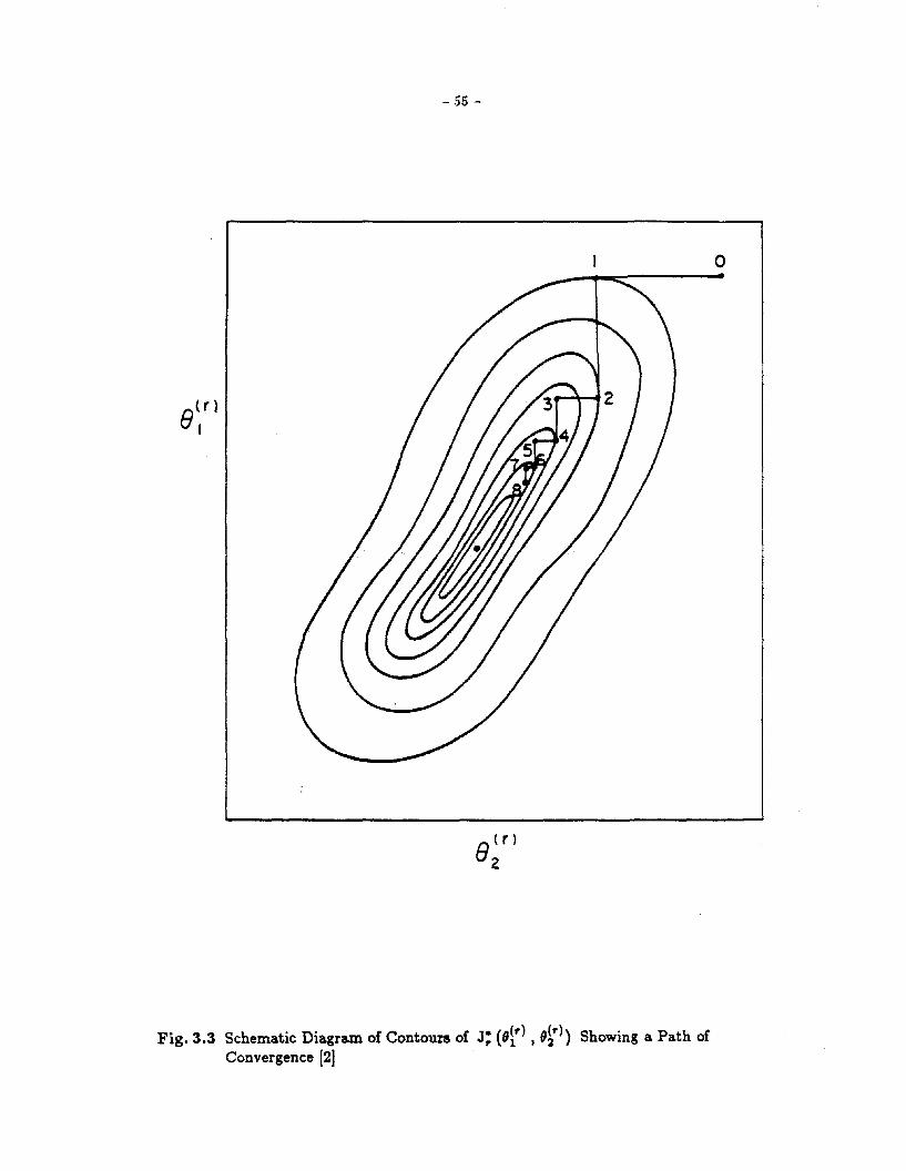
- 55-
o
Fig. 3.3 Schematic Diagram of Contours of J; (9~r) ,9~r» Showing a Path ofConvergence [2J

I 01
0) I
20
.01
6.0
12.
0(S
EC
)8
.0 TIM
E4.
0
II
II
RO
OF
--
.
.r.A
ItA
A~~
~vv
"~
--
II
II
20
.00
-20
.D
C{).
0
10
.00
~ u w Ul
"- L U ~
0.0
0>- I- ......
U E)
-l
W >-1
0.0
0
Fig
.3.4
Pse
udo-
Vel
ocit
ies
ofth
eT
est
Str
uct
ure
(-)
and
Cal
cula
ted
Vel
ocit
ies
ofa
Tw
o-M
ode
Mod
el(-
--)
,at
the
Roo
f,M
id-H
eigh
tan
dF
loor
2jM
odel
Iden
tifi
edfr
omV
eloc
ityR
ecor
ds
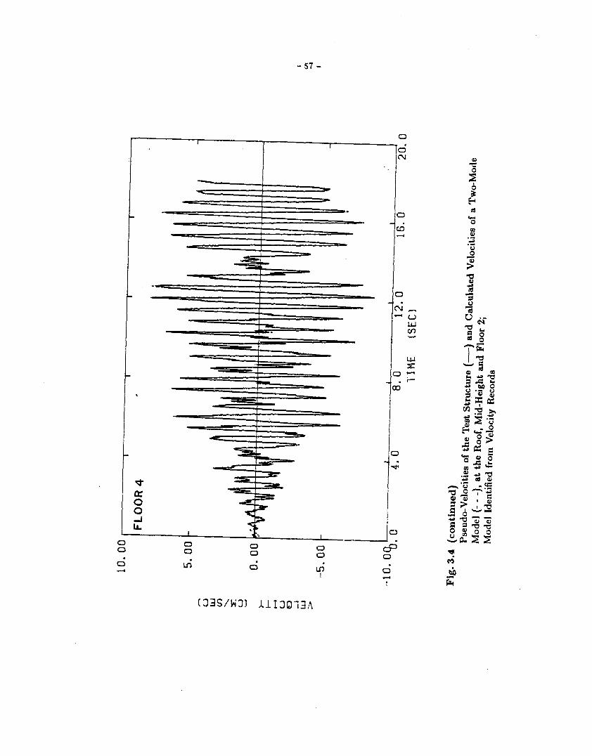
FL
OO
R4
10
.00
II
II
I1
u w (f) ":F. U
5.0
0to-
J-
}o
I- ......
U E)
-.J
W :>
O.
00rJ'~
1t1J
titt
tt.1
fitH
tl-t
#ml+
RiJ+
+U-I
-ill
W-Ui
ll
-5.
00
to-
-
I U1
-l I
jL
I16~0
--""2
0.0
-~n----T'0
--1
2.
0I
8.0
-10
.0%
.0-
4.0
liM
E(S
EC
]
Fig
.3
.4(c
on
tin
ued
)
Pse
udo-
Vel
ocit
ies
ofth
eT
est
Str
uct
ure
(-)
and
Cal
cula
ted
Vel
ocit
ies
ofa
Tw
o-M
ode
Mod
el(-
--)
,at
the
Roo
f,M
id-H
eigh
tan
dF
loor
2jM
odel
Iden
tifi
edfr
omV
eloc
ity
Rec
ords

.'
5.0
0r
II
II
II
FL
OO
R2
u w en .......
'E u > I-~ U o -l
W >
2.
50~
0.0
0
-2.
50
Ittl
- -
I Q1
00 I
--5.
eCh.
0I 4.0
I
8.0 TI
ME
I
12
.0
(SE
C)
I
16
.02
0.0
Fig
.3.4
(co
nti
nu
ed
)Ps
eudo
--V
eloc
itie
sof
the
Tes
tS
tru
ctu
re(-)
and
Cal
cula
ted
Vel
ocit
ies
of
aT
wo-
Mod
eM
odel
(--
-),
atth
eR
oof,
Mid
-Hei
ght
and
Flo
or2j
Mod
elId
enti
fied
from
Vel
ocity
Rec
ords

2.0
0r
II
II
I
RO
OF
1.0
0~
_II
1\l
l•
-,....
.:E U
III
/I
IIII
II...
nII
II
II
•
I-
r.;,
,fz
.Ai\
1\~
JI~
I
W :EO
.0
0~
VV
~V
V11
,1
11
11
11
11
11
11
.W U a: ...
.J
V
~~~ij~~~
II
CL0
1U
l<
0..-.
I0
-1.
00
r--
-2.
DCb.
0I 4.
0I
8.0 TI
ME
I
12
.a
(SE
C)
I
16
.0
20
.0
Fig
.3
.5M
easu
red
Dis
plac
emen
tso
fth
eT
est
Str
uct
ure
(-)
and
Cal
cula
ted
Dis
plac
emen
tsfo
rth
eS
ame
Tw
o-M
ode
Mod
elas
inF
ig.3
.4(-
--)
,at
the
Roo
f,M
id-H
eigh
tan
dF
loor
2

1.00
II
II
II
FL
OO
R4
O.
50~
II
•1\
IIII
III
I•
•-
,.....~
I1
11
1.j,
IIII
•U
~JI
,I-
ftz
.A/I.
1\A
aIw ~
0.0
0.
VV
VV
VI'
~w u a: -J lL
~\ijII
~~ij
II
(f)
0>
0t-
tI
a-0
.5
0-
-
-1.0~10
II
II~
4.0
8.0
12
.0
16
.02
0.0
TIM
E(S
EC
)
Fig
.3.5
(co
nti
nu
ed)
Mea
sure
dD
ispl
acem
ents
ofth
eT
est
Str
uct
ure
(--)
and
Cal
cula
ted
Dis
plac
emen
tsfo
rth
eS
ame
Tw
o-M
ode
Mod
elas
inF
ig.3
.4(-
--)
,at
the
Roo
f,M
id-H
eigh
tan
dF
loor
2
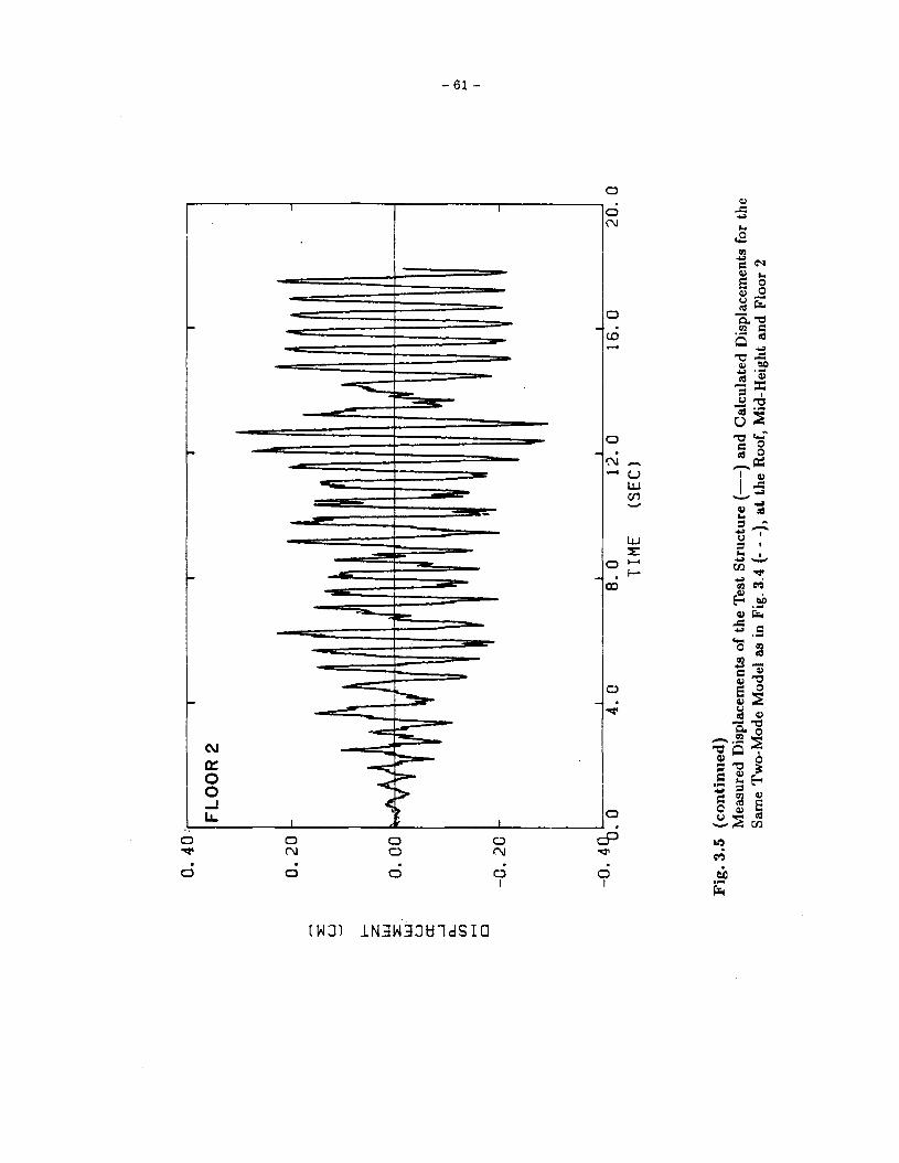
I 0) .....
20.
01
6.0
12
.0
(SE
C)
8.0 TI
ME
4.0
:I
II
I
FL
OO
R2
--
,It.
AA
I-H"VV~
~•
f-
II
II
0.4
0
-0.
4Cb.
0
0.2
0~ :£ U ~ l- Z W
0.0
0:£ W U a: -.
J n...
(f)
.......
0
-0.2
0
Fig
.3.5
(co
nti
nu
ed)
Mea
sure
dD
ispl
acem
ents
ofth
eT
est
Str
uct
ure
(--)
and
Cal
cula
ted
Dis
plac
emen
tsfo
rth
eS
ameTw~Mode
Mod
elas
inFi
g.3.
4(-
--)
,at
the
Roo
f,M
id-H
eigh
tan
dF
loor
2
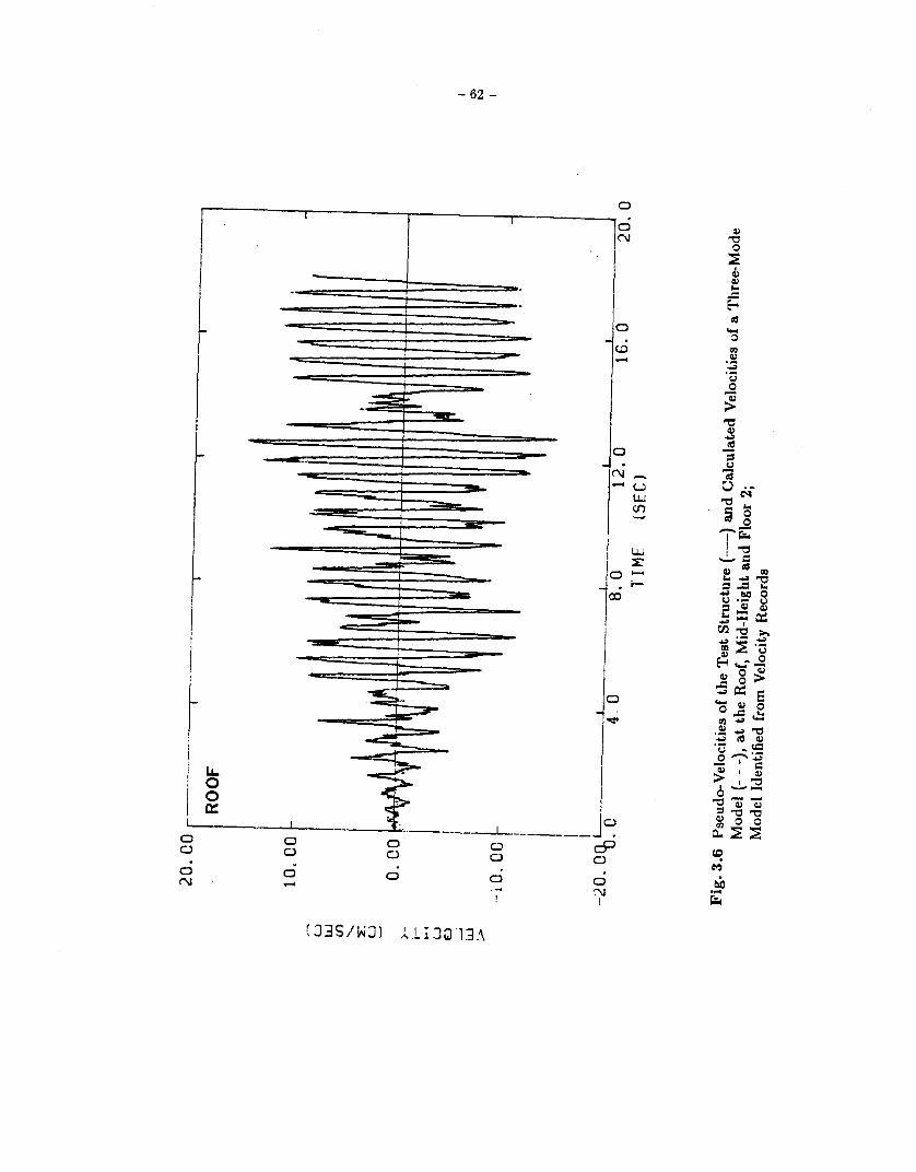
I 0>
N I
20
.01
6.0
12
.0(S
EC
)8
.0 TIM
E4
.0
~--
I-
II
I
ROO
F
.r
-
I ,
•
_"A
IlA
AI.~~
-
~"..
vvv
~.
I~
I I I ~.
-..
I I I I II
II
II
20
.00
'-20.
0Ch.
0
10
.00
~ u w (f) "~ u ~
0.0
0>- I-
t--<
U 0 -' w >-
--10
.00
Fig
.3.6
Pse
udo-
Vel
ocit
ies
ofth
eT
est
Str
uct
ure
(--)
and
Cal
cula
ted
Vel
ocit
ies
ofa
Thr
ee-M
ode
Mod
el(-
--)
,at
the
Roo
f,M
id-H
eigh
tan
dF
loor
2jM
odel
Iden
tifi
edfr
omV
eloc
ity
Rec
ords

10
.0
0I
IJ
II
1
FL
OO
R4
I 0> W I
20
.01
6.0
12
.0
(SE
C)
8.0 I·
IME
4.0
,
I
J-
l- II I
I
.~U
IA&
~~
~.'''~~
I'
~~
I•
-t-
•
II
I1
-io.
0en.a
5.0
0r-
-.
U l1J
if)
........
::i:
U -.J
O.00
~-
~- ..., u E)
-.J
l1J >
·-5.
00
Fig
.3.6
(co
nti
nu
ed
)
Pse
udo-
Vel
ocit
ies
ofth
eT
est
Str
uct
ure
(-)
and
Cal
cula
ted
Vel
ocit
ies
of
aT
hree
-Mod
eM
odel
(--
-),
atth
eR
oof,
Mid
-Hei
ght
and
Flo
or2j
Mod
elId
enti
fied
from
Vel
ocit
yR
ecor
ds

5.00
II
II
II
FL
OO
R2
2.5
0~ U l.J
J(f
) '- ~ u ~0
.00
>- I- ......
uI
'III
!'E
)
-l
l.JJ >
-2.
SO
I
-5C
tbL
----'.
.04
.08.
a TIM
E1
2.0
(SE
C)
16
.02
0.0
I 0> ~ I
Fig
.3.6
(co
nti
nu
ed)
Pse
udo-
Vel
ocit
ies
ofth
eT
est
Str
uct
ure
(-)
and
Cal
cula
ted
Vel
ocit
ies
of
aT
hree
-Mod
eM
odel
(--
-),
atth
eR
oof,
Mid
-Hei
ght
and
Flo
or2;
Mod
elId
enti
fied
from
Vel
ocit
yR
ecor
ds

I 0> '" I
II
IR
OO
I
~.
-
Ml
,fA
.A"i.
4J
~,
.VV~V
V11
~f-
2.0
0[----------.-
--------.
---F
1.00
~ :E U ...... .- z w
0.0
0:F
.W U a: -" (L U
l~I
0-1
.00
-2.0C
b~6-
4~0
II
II
8.0
12
.01
6.0
20
.0TI
ME
(SE
C)
Fig
.3.7
Mea
sure
dD
ispl
acem
ents
of
the
Tes
tS
tru
ctu
re(-)
and
Cal
cula
ted
Dis
plac
emen
tsfo
rth
eS
ame
Thr
ee-M
ode
Mod
elas
inF
ig.
3.6
(--
-).
at
the
Roo
f.M
id-H
eigh
tan
dF
loor
2

J 0> 0> I
I-\
jA
~
.II
AJ\I\~
~I
/,"
7"
VV~V
VV
I--
1.0
0I
IF
LO
OR
4
0.5
0~ :£ U ~ ~ z w
0.0
0~ w
·u a: -I
CL if)~ 0
-0.
50
-l.°C
b.o
1I
4.0
8.0T~ME
II
I1
2.0
16
.02
0.0
(SE
C)
Fig
.3.7
(co
nti
nu
ed
)M
easu
red
Dis
plac
emen
tsof
the
Tes
tS
tru
ctu
re(--)
and
Cal
cula
ted
Dis
plac
emen
tsfo
rth
eS
ame
Thr
ee-M
ode
Mod
elas
inF
ig.
3.6
(--
-),
at
the
Roo
f,M
id-H
eigh
tan
dF
loor
2
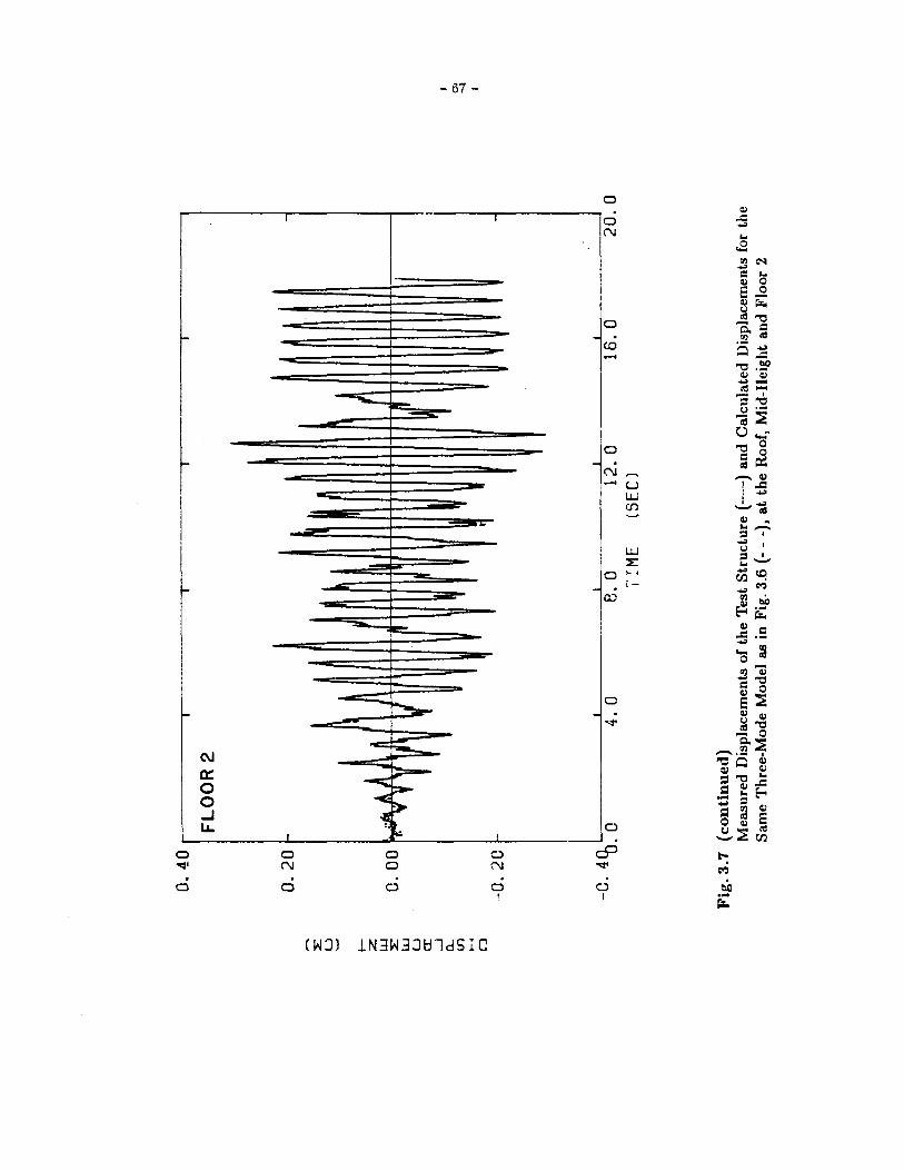
I 0> -l I
20
.01
6.0
12.a
(SE
C)
8.0 I~ME
4.0
II
II
FLO
OR
2
f--
··it
AA
ftJ
-rtf
"V1 •
~I
•f-
-
II
II
0.4
0
-0.
4£b.
0
0.2
0~ :E U .....
.
l- Z UJ
0.0
0:E U
JU a: ....
.J(L if)
~.
0
-0.
20
Fig
.3.7
(co
nti
nu
ed)
Mea
sure
dD
ispl
acem
ents
ofth
eT
est
Str
uct
ure
(-)
and
Cal
cula
ted
Dis
plac
emen
tsfo
rth
eS
ame
Thr
ee-M
ode
Mod
elas
inF
ig.
3.6
(--
-),
atth
eR
oof ,
Mid
-Hei
ght
and
Flo
or2

40
0.0
0I
II
II.
II
RO
OF
u w2
00
.00
(J)
"'- u w (J)
"'- ::i:
U
0.0
0
z E)
1-.
1
0: cr.
W ....
J-2
00
.0
0w u u c:
I ~
I 0>
00 I
I II
II
II
I-4
00
.0C
O.
01.
02
.0
3.
04.
05
.0
6.0
TIM
E(S
EC
)
Fig
.3
.8S
ix-S
econ
dS
egm
ents
of
the
Pse
udo-
Acc
eler
atio
n(-)
and
Cal
cula
ted
Acc
eler
atio
nU
sing
aT
hre
e-M
od
eM
odel
Iden
tifi
edfr
omP
seud
o-A
ccel
erat
ion
Rec
ord
(--
-),
at
Roo
f

f . .
4CO
.CO
rR
OO
F-
II
II
II
u UJ
20
0.0
0(f) " u UJ
(f) " ~ u
0.0
0
Z EJ
......,
i-'
a: a:-:
UJ
-J-2
00
.0
0U
JU L
J c::
I-4
00
.0c
t~0
7.0
11
8.0
9.0
TIM
E(S
EC
)
IJ
10
.0
-I
11
.0l' 2
.0
I 0> co I
Fig
.3.8
(co
nti
nu
ed)
Six
-Sec
ond
Seg
men
tso
fth
eP
seud
o-A
ccel
erat
ion(-)
and
Cal
cula
ted
Acc
eler
atio
nU
sing
aT
hree
-Mod
eM
odel
Iden
tifi
edfr
omP
seud
o-A
ccel
erat
ion
Rec
ord
(--
-),
atR
oof

I -'l
o I
18
.01
7.0
~6
.01
4.0
15
.0•.
!ME
(SE
C)
13
.0
IRO
OF
II
I-
II
l-f 'I
-
N~ I
I
V~
I
#v
I J..
I.
I:
•
Uij
&II
\~
~,
I,1
--II
,I
V~~VV
n..
~f
/:.
~.
'.0
:.
~I
~,,'
~~~
"
.',;
II
.\
I I
I-(
-
II
II
I
40
0.0
0
-40
0.
C\C2.
0
u2
00
.00
w (f) , u w (f) , ~ u
0.0
0
z 0 ...., 1·- a: Q~ w
-20
0.0
0-.
lw U u a:
Fig
.3.8
(co
nti
nu
ed)
Six
-Sec
ond
Seg
men
tso
fth
eP
seud
o-A
ccel
erat
ion(-)
and
Cal
cula
ted
Acc
eler
atio
nU
sing
aT
hree
-Mod
eM
odel
Iden
tifi
edfr
omP
seud
o-A
ccel
erat
ion
Rec
ord
(--
-),
atR
oof

30
0.
00
,,',
,,
II
RO
OF
u w (f) "
22
5.
00
I~ u
-
w a ~"
15
0.
00
I-II
11
-1
-1 -J ~I
'LII
~I
~a:: ~
75
.00
1-1
11
IHI
II-
a:: ~U~---U~
I''I
oOCL~~""""N!I
....'¥>WoIttojo,~
.~.
01
0.0
20
.03
0.0
40
.05
0.0
FRE
QU
EN
Cr
(HZ
)
Fig
.3.9
Fou
rier
Am
pli
tud
eS
pec
tru
mo
fP
seud
o-A
ccel
erat
ions
atR
oo
f
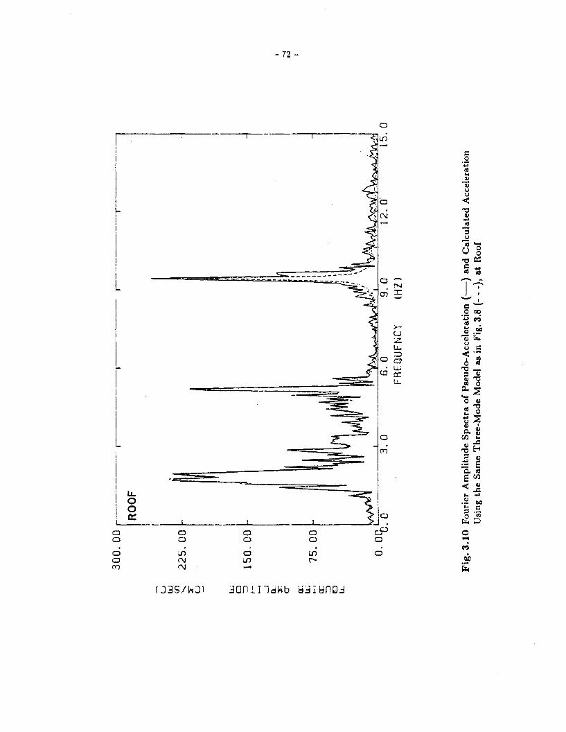
30
0.
00r R
O;----
I-----1
r-
J
lI
u
22
5.0
0f
w (/) "- L U
I,
\I
)I
iLL 0 :::
J1
50
.00
It-
o-;
II
-J
III
ll.-
II
L
j-'
Icr
,N
75
.0
0~
II
II
II
a::
LL 0-.
a:: ::J
0 IL
LJo
0Co
L..
:---_
__
----l
..0
3.0
Fig
.3
.10
Fou
rier
Am
pli
tud
eS
pec
tra
of
Pse
ud
o-A
ccel
erat
ion(-)
and
Cal
cula
ted
Acc
eler
atio
nU
sing
the
Sam
eT
hre
e-M
ode
Mod
elas
inF
ig.3
.8(-
--)
,at
Roo
f

-73 -
CHAPTER 4
SYSTEM IDENTIFICATION APPLIED TO THE ELASTIC
PSEUDO-DYNAMIC TEST DATA
_.TREATING FEEDBACK OF EXPERIl\1ENTAL ERRORS
4.1 Introduction
As discussed in the previous chapter, a straightforward application of a single-input
single-output system identification technique to estimate the modal properties of the full
scale six-story steel structure tested within its elastic range revealed negative damping for
the. third mode. This was attributed to the cumulative effect of feedback of control and
measurement errors during the pseudo-dynamic testing. These experimental errors were
analyzed in Chapter 2 and were shown to act as excitations to the structure in addition to
the ground motion.
In this chapter, these additional excitations are treated explicitly. For the purpose of
system identification, this requires a multiple-input multiple-output technique. An output
error technique, namely MODE-ID [1,2j, was used, which is applicable to any number of
simultaneous input excitations and structural response measurements used in conjunction
with a linear model. By accounting for the cumulative effect of the feedback of the ex
perimental errors during the estimation of the modal parameters of the structure from the
'elastic' test data, it is possible to estimate the actual structural damping effective during
the test and also the apparent equivalent viscous damping produced by the feedback errors.
The identification results from the full-scale structural test data are in good agreement with
the shaking table test results of a 0.3 scale model of the same prototype structure.
4.2 Modification of the Linear Structural Model
4.2.1 Analytical Model
It was shown in Chapter 2 that the cumulative displacement error '!?.f. is the response of
the structure to an excitation [ _K,!ec(t) - }!em(t) 1(Eq. 2.12), while the ideal (error-free)
displacement,!* is the response of the structure to aground excitation force [-ME(t) 1,]
(Eq.2.11). The total response '£ being the sum of both '£* and ,£e (Eq.2.10) suggests using

-74 -
the following differential equation as a structural model:
(4.1)
where E is the equivalent viscous damping in the model.
If the force measurement errors are negligible in comparison with the force effects of
displacement control errors as expected for a stiff structure, that is,
(4.2)
where II . \I is the Euclidean vector norm, then the structural model in Eq.4.1 can be
rewritten as:
M% + Ex + Kx = -Mz(t) 1- Kxec(t)f'!"W ,...",..", fI"'t<J""" (4.3)
H it is assumed, in addition, that the measurement errors in the displacements, xern.,.-
are much smaller than the displacement control errors, xec , that is,,.."
(4.4)
then from Eq. 2.8, xec can be calculated from known quantities, the measured and calculated,.."
displacements, as:
(4.5)
The time-histories of these displacement control errors during the Phase II elastic test are
plotted in Fig.4.1. At the roof, the peak displacement errors are about 1% of the peak
displacements and also the errors tend to oscillate at the fundamental frequency of the
structure.
For the reasons discussed in Section 3.3.1, a linear model based on the dominant modes
in the records of the response, and not on the stiffness and damping matrices as in Eq.4.3,
is preferred. This modal formulation is explained in the following section.
4.2.2 Modal Model
If the damping matrix E in Eq. 4.3 is assumed to be symmetric and also classical, then
arguments similar to the ones in Section 3.3.2 will ensure that M-1K and M-1E have a
common set of N orthonormal eigenvectors such that
M-1K~=~02
M-1E ~ =~ (2Z0)(4.6)

-75 -
where ~ = [tiP), ,p(2), ••• ,,p(N)], the modal column matrix of the structure normalized toI'<J _ I'<J
satisfy the following orthogonality relationships:
~T M~ = I, ~T K~ = 0 2 and ~T E~ = 2zn . (4.7)
Since the eigenvectors ,per) are a basis for N-dimensional vector spa.c::e R N , x can be written- --as
x(t) =~ e(t) ,- - (4.8)
where eis the vector of modal response amplitudes, that is the coordinates of x with respect- --to the basis of eigenvectors.
Substituting Eq.4.8 into Eq.4.3:
Premultiplying Eq.4.9 by ~T and using Eq.4.7:
e+ 2Z 0 e+n2e= -~TMz(t) 1 - ~T Kxec(t)~ ,...",..", ,...",..."
=-,2z(t) - B~ec(t) ,
or in component form:
e(r) + 2~(r) w(r) e(r) +w(r):I e(r) = _a(r) z(t) _ (3(r)T ~ec(t) ,-
(4.9)
(4.10)
where a(r) and /3(r) are the modal participation factors conesponding to the ground aeeel--erations and control-errors in displacements, respectively.
Equation 4.8 can also be written as:
N
~(t) =L: ~(r) (t) ,r=l
(4.11)
where (4.12)
and £(r) (t) is the contribution of the r-th mode to the response vector £(t).
From Eqs.4.10 and 4.12 the following equation can be deduced:
x(r) + 2~(r) w(r) i(") +w(,.):1 x(,.) = _",Cr) (aC") z(t) + (3C,.)T xec(t))""*"I ~ ~,..", ,..., ~
= -pC") J(t) , (4.13)IV

-76 -
where
[
z(t) ]f(t) = - - ---- ~ec(t)
and
p(r) :::: q;(r) [a(r) I p(r)T 1-- .....
(4.14)
is the effective participation factor matrix for the r-th mode.
In summary, the model used is Eqs.4.13 and 4.14 in conjunction with Eq.4.11. Hence
the parameters of the modal model to be estimated are:
{w(r), ~(r), p(r) : r= 1,2, ... ,N}
The effective participation factors and hence the mode shapes can be determined from the
first column of the matrices p(r).
4.3 Multiple-Input Multiple-Output (MI-MO) System
Identification Technique
The modal parameters corresponding to the linear model in Eq.4.13 are estimated
using a multiple-input multiple-output system identification technique which is applicable
to any elastic structure with any arbitrary configuration, classical normal modes, any num
ber of simultaneous excitations and structural response measurements, and an initial at-rest
position. This output-error technique was developed by Beck [1,2J to identify the pseudo
static and normal mode parameters of a linear model that characterized the measured
response of the Meloland Road Overpass during the 1979 Imperial Valley earth.quake.
The modal parameters O(r) to be estimated are:,..,.
w(r) -~(r) -
Pii(r) -
natural frequency of mode r I
damping ratio of mode r ,effective participation factor for mode r corresponding to thei-th response degree of freedom and the j-th excitationdegree of freedom: i =1," . ,NR
j = 1,···,NI
where
and
NR - no. of degrees of freedom at which the response is measured,
NI - no. of degrees of freedom at which the input excitation forces
are measured.
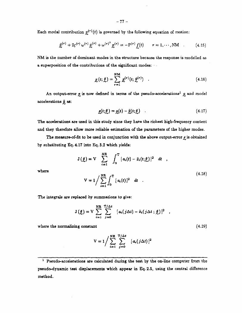
-77 -
Each modal contribution ~(r)(t) is governed by the following equation of motion:
r= 1, .. ·,NM . (4.15)
NM is the number of dominant modes in the structure because the response is modelled as
a superposition of the contributions of the significant modes: . .
·NM
:z:(t· 9) = ~ :z:{rl(t· 8(r l)"'I ',..."" L.J f'It,J ,~
r=l
(4.16)
An output-error ~ is now defined in terms of the pseudo-accelerations1 ~ and model
accelerations z as:-~(tj1') = !,(t) - !(tjPJ . (4.17)
The accelerations are used in this study since they have the richest high-frequency content
and they therefore allow more reliable estimation of the parameters of the higher modes.
The measure-of-fit to be used in conjunction with the above output-error e is obtained-by substituting Eq.4.17 into Eq. 3.2 which yields:
NR
J(PJ=V Li=1
where
The integrals are replaced by summations to give:
NR T/At
JCt)=V L L [a.(j6.t)-z.(j6.tj!)]2 ,i=1 ;=0
(4.18)
where the normalizing constant (4.19)
/
NR T/At
V=l L Li=l i=O
1 Pseudo-accelerations are calculated during the test by the on-line computer from the
pseudo-dynamic test displacements which appear in Eq.2.5, using the central difference
method.
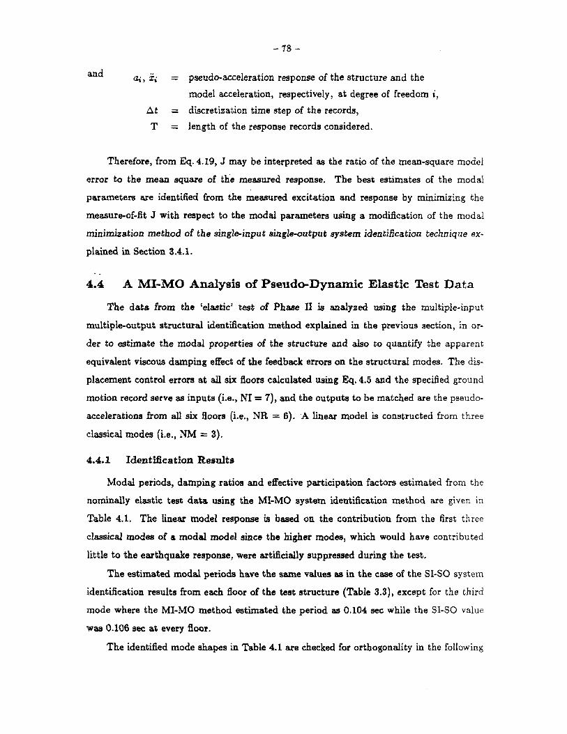
and
-78 -
a;, Xi - pseudo-acceleration response of the structure and the
model acceleration, respectively, at degree of freedom i,
6.t = discretization time step of the records,
T = length of the response records considered.
Therefore, from Eq. 4.19, J may be interpreted as the ratio of the mean-square model
error to the mean square of the measured response. The best estimates of the modal
parameters are identified from the measured excitation and response by minimizing the
measure-oi-fit J with respect to the modal parameters using a modification of the modal
minimization method of the single-input single-output system identifica.tion technique ex
plained in Section 3.4.1.
4.4 A MI-MO Analysis of Pseudo-Dynamic Elastic Test Data
The data from the 'elastic' test of Phase II is analyzed using the multiple-input
multiple-output structural identification method explained in the previous section, in or
der to estimate the modal properties of the structure and also to quantify the apparent
equivalent viscous damping effect of the feedback errors on the structural modes. The dis
placement control errors at all six floors calculated using Eq.4.5 and the specified ground
motion record serve as inputs (i.e., NI =7), and the outputs to be matched are the pseudo
accelerations from all six floors (i.e., NR = 6). A linear model is constructed from three
classical modes (i.e., NM == 3).
4.4.1 Identification Results
Modal periods, damping ratios and effective participation factors estimated from the
nominally elastic test data using the MI-MO system identification method are given in
Table 4.1. The linear model response is based on the contribution from the first three
classical modes of a modal model since the higher modes, which would have contributed
little to the earthquake response, were artificially suppressed during the test.
The estimated modal periods have the same values as in the case of the 51-SO system
identification results from each floor of the test structure (Table 3.3), except for the third
mode where the MI-MO method estimated the period as 0.104 sec while the 51-SO value
was 0.106 sec at every floor.
The identified mode shapes in Table 4.1 are checked for orthogonality in the following
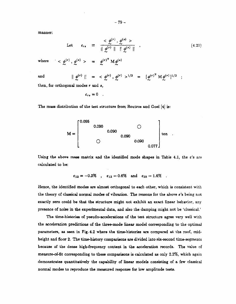
-79 -
manner:
where
and
< ¢J(r) , ¢J(3) >Let '" '" (4.20)er3 - II ¢J(r) II II ¢J(3) II
'" '"
< ¢J(r) , ¢J(3) > = ¢J(r)T M¢J(3)
'" '" '" '"
II ¢J( r) II = < ¢J(r) , ¢J(r) >1/2 = [¢J(r)T M ¢J(r) P/2'" '" '" '" '"
then, for orthogonal modes r and 8,
er3 = 0 .
The mass distribution of the test structure from Boutros and Goel [4] is:
M=
0.0950.090
o0.090
0.090
o
0.0900.077
ton .
Using the above mass matrix and the identified mode shapes in Table 4.1, the e'S are
calculated to be:
e12 = -0.3% , e13 =0.6% and e23 = 1.6% .
Hence, the identified modes are almost orthogonal to each other, which is consistent with
the theory of classical normal modes of vibration. The reasons for the above e's being not
exactly zero could be that the structure might not exhibit an exact linear behavior, any
presence of noise in the experimental data, and also the damping might not be 'classical.'
The time-histories of pseudo-accelerations of the test structure agree very well with
the acceleration predictions of the three-mode linear model corresponding to the optimal
parameters, as seen in Fig. 4.2 where the time-histories are compared at the roof, mid
height and floor 2. The time-history comparisons are divided into six-second time-segments
because of the dense high-frequency content in the acceleration records. The value of
measure-of-fit corresponding to these comparisons is calculated as only 2.2%, which again
demonstrates quantitatively the capability of linear models consisting of a few classical
normal modes to reproduce the measured response for low amplitude tests.

- 80-
The analytical model used to represent the structure during the MI-MO system iden
tification procedure is:
Mi + Ex + Kx = -Mz(t) 1 - Kxec(t)"""'J f1I"<J""'" I"'t.tI ~
(4.21)
Since the effects of the experimental errors are now explicitly taken into account as excita
tions to the structure in addition to the ground accelerations, the viscous damping matrix
E in Eq. 4.21 will represent the sum of the viscous damping from the computer algorithm (C
in Eq.3.30), and the structural damping effective during the test. These various damping
values are estimated in the following section.
4.4.2 Estimation of Structural Damping and Equivalent Viscous
Damping Effect of Experimental Errors
The following is summarized from the previous sections in order to estimate damping
values corresponding to both the structure and the effect of experimental errors.
The equation of motion of the test structure used in the pseudo-dynamic method is:
where [C J= [Algorithmic Damping J
(4.22)
(4.23)
The analytical model used in the SI-SO system identification method is:
Mi+ Dx+ Kx = -Mz(t) 1 ,"...., ,...",..", ,...,.,
where
[D] = [C] + [Structural Damping] + [Feedback Error 'Damping']
Similarly, the analytical model used in the MI-MO system identification method is:
Mi + Ex + Kx = -Mz(t) 1- Kxec(t)~ """'J""'" ,....,,....,
(4.24)
(4.25)
(4.26)
where [E] = [C] + [Structural Damping1 (4.27)

- 81-
Therefore, from Eqs. 4.25 and 4.27,
[Structural Damping] = [E] - [C]
[Feedback Error Damping] = [D] - [E]
(4.28)
(4.29)
The algorithmic damping C used in the on-line computer calculations during the actual
pseudo-dynamic test was constructed using the specified diagonal modal damping matrix
Z1 based on Table 3.5, and the modal frequencies 0 1 and modeshapes <1>1 obtained from a
pre-test finite element analysis of the test structure [4] as follows:
(4.30)
Since the effective natural frequencies 0 and modeshapes <1> of the structure during the
test, as identified by the MI-MO method, are different from the pre-test analytical val
ues, the effective modal damping matrix Zz corresponding to the algorithmic damping is
reconstructed as follows:
(4.31)
Although Z1 is a diagonal matrix, Zz need not be, since the stiffness matrix effective during
the elastic pseudo-dynamic test is different from its pre-test analytical value. Z2 calculated
as above is shown in Table 4.2 and is approximated by its diagonal elements alone. Since
only the first three modes were identified using the MI-MO method, the pre-test modeshapes
were used in <1> for the last three modes. This is why the diagonal modal damping values
above the third mode remain unchanged.
The above modal damping values for C which are different from the values in Table
3.5 for. the first three modes, and modal damping values for D and E from SI-S0 and
MI-MO results, respectively, are shown in the first three columns of Table 4.3. The struc
tural damping and feedback error damping values of the first three modes calculated using
Eqs. 4.28 and 4.29, respectively, are shown in the last two columns of Table 4.3.
The low structural damping values ofless than 1% as shown in Table 4.3, compared to
field observations of 3% to 8% for the earthquake response of actual buildings, are mainly
due to the absence of nonstructural components in the test structure and the absence of
radiation damping during the pseudo-dynamic test because of its quasi-static nature.

- 82-
Feedback errors have produced' positive damping values of 0.3% and 0.9% in the first
two modes, and a negative damping value of 2.4% in the third mode, confirming the fact that
higher modes are affected significantly by the feedback of experimental errors in pseudo
dynamic testing. More than 2% of negative feedback damping in the third mode, which
is about 4 times larger than the positive structural damping in that mode, explains the
extraordinarily strong third-mode signal seen in Fig. 3.9.
4.4.3 Comparisons of Full-Scale and Scale-Model Test Results
The full-scale structural identification results of natural frequencies, damping ratios
and modeshapes using MI-MO technique are compared in Table 4.4 and Fig. 4.3, with the
corresponding results from a 0.305 scale-model of the same prototype structure tested on
a shaking table at the University of California, Berkeley by Bertero, et al. [5].
In Table 4.4, model periods have already been scaled up by 1/YO.305 so that they can
be compared with the full-scale structural values. Also, the plotted mode shape vectors for
the full-scale structure are just the effective participation factors in Table 4.1 , which in
turn are the first column of each modal participationfactor matrix p(r), r =1,2,3, appearing
in Eq.4.13.
The periods and modeshapes of both the full-scale structure and the scale model are
in good agreement and the small difference in the damping values could be attributed to
radiation and table-structure interaction effects present in the shaking table test. Overall,
the scale-model test proved to be a viable alternative to full-scale testing, at least with
regard to reproducing the modal properties of the full-scale structure.
4.4.4 Conclusions
A linear model consisting of three classical normal modes was shown to be capable
of reproducing the measured structural response with a mean-square acceleration error of
2% of the mean-square pseudo-acceleration. Also, it was shown that the effect of feedback
errors may be accounted for when estimating the modal parameters. By using the control
errors, in addition to the ground motion, as inputs to a multiple-input multiple-output
system identification technique, the equivalent viscous dampings for energy dissipated by
the structure and for the apparent damping from the feedback errors were estimated. The
identification results showed that the feedback errors added energy to the test structure in
its third mode but damped the contributions of the first two modes during the nominally

- 83-
elastic test of Phase II.
The estimates for the modal parameters of the full-scale structure are in very good
agreement with those from a 0.3 scale model tested on a shaking table, suggesting that
scale-model testing is in fact a reliable technique for reproducing the dynamic properties
of full-scale structures.

- 84-
REFERENCES
[1] Werner, S.D., Levine, M.B. and Beck, J .L., "Seismic Response Characteristics ofMeloland Road Overpass During 1979 Imperial Valley Earthquake," Report No. R8222-5603, Agbabian Associates, EI Segundo, California, March, 1985.
[21 Beck; J.L., "Users Guide for MODE-ID," Report No. R-8222-5931, Agbabian Associates, EI Segundo, California, March, 1985.
[3] Beck, J.L. and Jayakumar, P., "System Identification Applied to Pseudo-Dynamic TestData: A Treatment of Experimental Errors," Proceedings of the 9rd ASCE EngineeringMechanics Specialty Conference on Dynamic Response of Structures, University ofCalifornia, Los Angeles, California, April, 1986.
[41 Boutros, M.K. and Goel, S.C., "Pre-Test Analysis of the Six-Story Eccentric-BracedSteel Test Building," Proceedings of the 5th Joint Technical Coordinating CommitteeMeeting, U.S.-Japan Cooperative Research Program Utilizing Large-Scale TestingFacilities, Tsukuba, Japan, February, 1984.
[5] Bertero, V., et al., "Progress Report on the Earthquake Simulation Tests and Associated Studies of 0.3 Scale Models of the 6-story Steel Test Structure," Proceedingsof the 6th Joint Technical Coordinating Committee Meeting, U.S.-Japan CooperativeResearch Program Utilizing Large-Scale Testing Facilities, Maui, Hawaii, June, 1985.

- 85-
Mode Period (sec) Damping (%)
1 0.553 0.90
2 0.191 1.19
3 0.104 2.32
Effective Participation Factor
Mode at Floor
2 3 4 5 6 Roof
1 0.30 0.53 0.78 1.01 1.22 1.40
2 0.37 0.48 0.42 0.16 -0.19 -0.53
3 0.15 0.11 -0.05 -0.17 -0.05 0.15
Table 4.1 Modal Parameters Estimated from the PseudoAcceleration Records Using a Three-Mode Model and the MI-MOTechnique (J=2.2%) [3]
0.33 0.00 0.00 0.00 0.00 0.000.03 0.31 0.01 0.00 0.00 0.00
Z2=0.37 0.35 1.75 0.00 0.00 0.00
-1.12 2.55 -0.33 90.00 0.00 0.004.64 -1.00 -0.85 0.00 90.00 0.00
-0.67 -3.33 -0.66 0.00 0.00 90.00
Table 4.2 The Effective Modal DampingMatrix Z2 Corresponding to the AlgorithmicDamping C, as in Eq.4.31 (values in percentof critical)

- 86-
Damping (%)
Mode Numerical SI-S0 MI-MO FeedbackStructural
[C] [D] [EI Errors1 0.33 1.23 0.90 0.33 0.58
2 0.31 2.11 1.19 0.92 0.88
3 1.75 -0.05 2.32 -2.37 0.56
Table 4.3 Estimated Damping Values
Period (sec) Damping (%)Mode Structure Scale Model Structure Scale Model
1 0.553 0.572 0.58 0.672 0.191 0.190 0.88 0.903 0.104 0.105 0.56 -
Table 4.4 Comparison of Modal Period and Damping Values for Full-ScaleStructure and Scale-Model Specimen

I 00~ I
18.
01
5.0
12
.06
.09
.0T
IME
(SE
C)
3.0I
II
II
ROOF
I--
~M~
,~I
II
~l-
II
II
I--
-
40
.00
-40
.0C
b.0
20
.00
L U .., '0 ......
a: 0 a:0
.00
a: w -I
0 a: ~- z 0
-20
.00
u
Fig
.4.1
Tim
e-H
isto
ries
ofD
ispl
acem
ent
Con
trol
Err
ors
atth
eR
oof,
Mid
-Hei
ght
and
Flo
or2

10
.00
rI
II
Ii-----,
FLO
OR
4
5.0
0L~u
II11
111U
I1'0 cr
.II
'I'If'
"D cr:
O.00
f-'
Mcr
. w
I-l
l~W
D cr. i-
n1~
fJIf'
II"i"lr
111fiI
WIll
/I
z0
0D
00
u-5
.00
, I.
~iO.OC
bl-!
-!
II
I3.
a6
.09
.01
2.0
15
.01
8.0
."IM
E(S
EC
)
Fig
.4.1
(co
nti
nu
ed)
Tim
e-H
isto
ries
of
Dis
plac
emen
tC
ontr
olE
rro
rsat
the
Roo
f,M
id-H
eigh
tan
dF
loor
2

10
.0
0I
II
II
I,
FLO
OR
2
5.0
04
rt>U
'0 .~ a: 0 ~
0.0
0W -J 0 cr
: ~-5
.00l
'11 111
11tI
'lrI"
"r
II,,
'I'IIJI
/II',
"'/11
rII~"
~,,
11 1'1~lJ
I 00
10 I
-10
.0C
o.0
3.0
6.0
9.0
TIM
E(S
EC
)1
2.0
15
.01
8.0
Flg
.4.1
(co
nti
nu
ed)
Tim
e-H
isto
ries
ofD
ispl
acem
ent
Con
trol
Err
ors
atth
eR
oof,
Mid
-Hei
ght
and
Flo
or2

40
0.
00I
I----
----
----
----
------
r----
----
----
---,
----
-
RO
OF
o.OO~Jo~
Z Du w2
00
.00
(f)
......
u w (f)
......~ u I
IT a:: w -'-2
00
.0
0w u U 0
:
I <D o I
-40
0.0Cb~o-
L 1.0
__
l-_
__
L._
__
__
...l
_._
..L
..
_
2.0
3.0
4.0
5.0
6.0
TIM
E(S
EC
)
Fig
.4.2
Pse
udo-
Acc
eler
atio
nso
fth
eT
est
Str
uct
ure
(-)
and
Cal
cula
ted
Acc
eler
atio
nsof
aT
hree
-Mod
eM
odel
(--
-»at
the
Roo
f)M
id-H
eigh
tan
dF
loor
2jM
odel
Iden
tifi
edfr
omP
seud
o-A
ccel
erat
ion
Rec
ords

I <0~
12.
01
1.
0-
10.
0B
.O9
.0T
IME
(SE
C)
7.0
~--
-_._
----
-,--------T
--
II
I
RO
OF
~-
~I~
.M
~~
IIIf
~~~
__
_L_~
_-
[-
--
_.
.-
~Nv
IVI
NV
.~
~\
~
._..
l._
....._
__
_...
.L_
_.
I.L
-:c-"
40
0.0
0
-40
0.
Des
.0
u2
00
.00
lJ.J
(f)
....... u w (f) "- ~ u
o.00
z 0 ......
I-
IT (r w
-20
0.0
0-J w U U IT
Fig
.4.2
(co
nti
nu
ed)
Pse
udo-
Acc
eler
atio
nso
fth
eT
est
Str
uct
ure
(-)
and
Cal
cula
ted
Acc
eler
atio
nso
fa
Thr
ee-M
ode
Mod
el(-
--)
,at
the
Roo
f,M
id-H
eigh
tan
dF
loor
2jM
odel
Iden
tifi
edfr
omP
seud
o-A
ccel
erat
ion
Rec
ords

40
0.0
0R
OO
F
----
----
-T--
----
---
-------
r----
-.------------,
-40
0.~~~-d-
__
__
__
_1
_
13.
0_
_L
..L1
L_
14
.0
15
.0
1G.
01
7.
0.
18.a
TIM
E(S
EC
)
Fig
.4.2
(co
nti
nu
ed)
Pse
udo-
Acc
eler
atio
nso
fth
eT
est
Str
uct
ure
(--)
and
Cal
cula
ted
Acc
eler
atio
nsof
aT
hree
-Mod
eM
odel
(--
-),
atth
eR
oof,
Mid
-Hei
ght
and
Flo
or2;
Mod
elId
enti
fied
from
Pse
udo-
Acc
eler
atio
nR
ecor
ds

20
0.0
0F
LO
OR
4
--I"
---.
---_
._-
---
----T---------~---
--.-
-------
I-----,
w1
00
.00
UJ
({) "w UJ
({) "~ w
0.0
0
Z D .......
I- a: a: UJ
-10
0.0
0....
JU
JW W a:
IL
__-2
00
.0C
O~-d
1.0
ii
___L
___
L._
_L0_
1-
_
2.a
3.0
4.0
5.0
6.0
TIM
E(S
EC
)
I <0
c,.
) I
Fig
.4.2
(co
nti
nu
ed)
Pse
udo-
Acc
eler
atio
nso
fth
eT
est
Str
uct
ure
(-)
and
Cal
cula
ted
Acc
eler
atio
nso
fa
Th
ree-
Mo
de
Mod
el(-
--)
,at
the
Roo
f,M
id-H
eigh
tan
dF
loor
2;M
odel
Iden
tifi
edfr
omP
seud
o-A
ccel
erat
ion
Rec
ords

I(0 ,p.. I
12
.01I.
010
.0
B.0
9.
0T
IME
(SE
C)
7.0
~~
II
II
I
FL
OO
R4
II
f-I
Ii~
~~j
tI~
~N
~~
-
~\\
A~
~~
~,
•
II
II
II
20
0.0
0
-20
0.
Oct
.0
u1
00
.00
w (f) ......
u w (f) ......~ u
0.0
0
Z fJ >-t r- IT a: w
-10
0.0
0-l w U U IT
Fig
.4.2
(co
nti
nu
ed)
Pse
udo-
Acc
eler
atio
nso
fth
eT
est
Str
uct
ure
(-)
and
Cal
cula
ted
Acc
eler
atio
nso
fa
Thr
ee-M
ode
Mod
el(-
--)
,at
the
Roo
f,M
id-H
eigh
tan
dF
loor
2;M
odel
Iden
tifi
edfr
omP
seud
o-A
ccel
erat
ion
Rec
ords

20
0.0
0F
LO
OR
4
U III
10
0.
00
({)
.......
U lI.J
(()
.........
.:E UO
.0
0~
-->
---------.-
-
Z D I IT oc: 'j
-)0
0.
00
w u U IT
I--
---.
----
----
----
-T--
----
--
----
--,-
-.--
----
--
I <0 en I
-20
0.
qa;~-
------
f3~O-
__._
1_
...
..1.
...-
.-.._
_L...
L.
._.
.
14
.01
5.0
16
.01
7.0
18
.0T
IME
(SE
C)
Fig
.4.2
(co
nti
nu
ed)
Pse
udo-
Acc
eler
atio
nso
fth
eT
est
Str
uct
ure
(-)
and
Cal
cula
ted
Acc
eler
atio
nso
fa
Thr
ee-M
ode
Mod
el(-
--)
,at
the
Roo
f,M
id-H
eigh
tan
dF
loor
2;M
odel
Iden
tifi
edfr
omP
seud
o-A
ccel
erat
ion
Rec
ords

20
0.
00
r.
IFL
OO
R2
I'-~
--"
----
II
iI
f--- ;
-IOO
oool
~!
I <0 en I
w U u a:
-20
0.0Cb~d
----
---l
-~O-
--__
____
___1
..__
1..
1..__
__
t__~---~---~--
2.0
3.0
4.0
5.0
6.0
TIM
E(S
EC
)
Fig
.4.2
(co
nti
nu
ed)
Pse
udo-
Acc
eler
atio
nsof
the
Tes
tS
tru
ctu
re(--)
and
Cal
cula
ted
Acc
eler
atio
nsof
aT
hree
-Mod
eM
odel
(--
-),
atth
eR
oof,
Mid
-Hei
ght
and
Flo
or
2;M
odel
Iden
tifi
edfr
omP
seud
o-A
ccel
erat
ion
Rec
ords
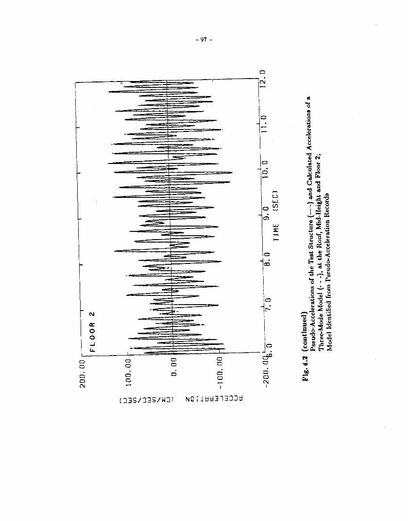
I <0~ I
12
.011
.0
10.
08
.09
.0T
IME
(SE
C)
7.0
.....-
II
-1I
I
FLO
OR
2
I
~.
-,
.
.~
~• 1\
II"
V~
,•
-I
-I
II
II
--2
00
.0c
tJ.
0
20
0.0
0
u1
00
.00
w (f) ..... u w (f) ..... ~ u
0.0
0
Z D ......
f- a: a:: w
-10
0.0
0_
J w U u a:
Fig
.4.2
(co
nti
nu
ed)
Pse
udo-
Acc
eler
atio
nso
fth
eT
est
Str
uct
ure
(--)
and
Cal
cula
ted
Acc
eler
atio
nso
fa
Thr
ee-M
ode
Mod
el(-
--)
,at
the
Roo
f,M
id-H
eigh
tan
dF
loor
2;M
odel
Iden
tifi
edfr
omP
seud
o-A
ccel
erat
ion
Rec
ords

I cD 00 I
t8.
0t7
.0
1G.
01
4.0
15
.0TI
ME
(SE
C)
13
.0
.---
----
-T-
----
------I
FL
OO
R2
I---
.-----
-I
_.-
--
n
~
. ~
~I
;)
J~l~
~-If
~-..
n
~v~
VI
~II
II\
I,.t
(
~
----
--_
.---
II
__
__
.J.
20
0.0
0
-20
0.
QC2.
0
u1
00
.00
UJ en ....... u UJ en .......~ u
0.0
0
z 0 .-.
I--
IT-
a::
UJ
-10
0.0
0--
lU
JU U IT
-
Fig
.4.2
(co
nti
nu
ed)
Pse
udo-
Acc
eler
atio
nsof
the
Tes
tS
tru
ctu
re(-)
and
Cal
cula
ted
Acc
eler
atio
nsof
aT
hree
-Mod
eM
odel
(--
-),
atth
eR
oof,
Mid
-Hei
ght
and
Flo
or2j
Mod
elId
enti
fied
from
Pse
udo-
Acc
eler
atio
nR
ecor
ds

RO
OF
4+
:14
--
SY
ST
EM
IDE
NT
IFIC
AT
ION
(MI-
MO
)
3t
)3t'\
I
3f
I----
0.3
SC
ALE
MO
DE
LT
ES
T'" '" I
2~
IF
LOO
R2
~I
FLO
OR
2
5
FLO
OR
6
RO
OF
FU
ND
AM
EN
TA
LM
OD
ES
EC
ON
DM
OD
ET
HIR
DM
OD
E
Fig
.4.3
Com
pa.r
ison
of
Mod
esha
.pes
for
Full-
Sca.
leS
tru
ctu
rean
dS
ca.le
-Mod
elS
peci
men

-100 -
CHAPTER 5
MODELING OF HYSTERETIC SYSTEMS
5.1 Ilitroduction
The problem of designing structures to resist the vibratory forces developed by strong
earthquake ground motions leads naturally to the investigation of the response of structures
that are stressed beyond the yield point into the nonlinear range [1]. In essence, this
requires a method for describing the dynamic force-deflection relation of the structural
members right up to their ultimate strength. Because the restoring force of such a system
is highly nonlinear and depends not only on the instantaneous displacement, but also on
its past history, analytical modeling of such a system under arbitrary excitation has been
a challenging and interesting subject [21.
Force-deformation relations can be obtained from the constitutive equations which
govern material behavior at a point, but complex stress distributions and material in
homogeneities render such an approach impractical. In addition, there is not a common
agreement on the choice of such constitutive models. On the other hand, force-deformation
relationships tend to be different in character from the underlying constitutive equations,
as they reflect the behavior of the member as a whole and also include geometrical effects
[3].
Elastic-perfectly plastic and bilinear hysteretic models have been studied extensively in
the past, mainly because of their simplicity. But for dynamic studies it would be desirable
to use a yielding relation that has a deviation from linearity which is smooth and yet is
general enough to describe yielding behavior varying within a wide range. Such a relation
would be a more realistic model for most practical applications, since even materials with
a sharply pronounced yield point in tension exhibit smooth force-deflection relations when
formed into structural shapes. Furthermore, an assemblage of structural shapes can, in
general, be expected to exhibit a rounded force-deflection curve [11.
In this chapter, various nonlinear hysteretic models are discussed within this context
and finally a simple model which is consistent with the real behavior of several materials
and structures under dynamic loading conditions is presented.

- 101-
5.2 A General Class of Masing Models
5.2.1 Masing's Hypothesis
Masing, in a paper titled "Self Stretching and Hardening for Brass" in 1926 [41, assumed
that a metal body consists of a system of body elements each with the same elastic stiffness
but different yield limits, and that the force-deformation curve of such an element, as shown
in Fig. 5.1, consists of two straight lines.
Masing then asserted that if the load-deflection curve for the entire system at the virgin
loading is symmetric about the origin and is given by
I(%,r) =0 (5.1)
where % is the displacement and r is the restoring force, then the unloading and reloading
branches of the hysteresis loops for steady-state response are geometrica.lly similar to the
virgin loading curve and are described by the same basic equation except for a two-fold
magnification. Applying this to a hysteretic loop describing cyclic loading between (%0, ro)
and (-%0, -ro) as shown in Fig. 5.2, each branch of the hysteresis loop is given by:
(
% - %* r - r*)1 2'~ =0 , (5.2)
where (%*, r*) is the load reversal point for that particular branch curve. Therefore, the
descending (unloading) branch of the hysteresis loop becomes
1( %0 - % !:!?..=.!:) = 02 ' 2 '
while the ascending (reloading) branch of the hysteresis loop becomes (5.3)
1( % ~%0 , r ~ ro ) = 0 .
T? experimentally test these equations, brass rods of different preliminary treatment
were first plastica.lly extended and then compressed. The overa.ll result of Masing's exper
iment was that the compression curve obtained fran the experiment deviated only a little
from the compression curve computed from Eq. 5.2, with 1(%, r) based on the initial tension
curve. This showed that the model is in agreement with the well known Bauschinger effect
occurring in a metal, which describes the weakening of the metal in one loading direction
due to plastic ~ing in the opposite direction during cyclic loading as observed in his
experiment.

- 102-
The Bauschinger effect, also observed in soils, is usually attributed to damage caused
in the material by the initial stressing (slips along crystal planes in a solid; slips between
grains in a soil). Prager devised a simple mechanical model to demonstrate this; it is a
kinematic model, and the increased strength on straining and the Bauschinger effect are
therefore sometimes referred to as kinematic hardening [5].
5.2.2 Properties of Masing Hysteresis Loops for Steady-State Response
The following are some of the important properties of the Masing hysteresis loops
which were discussed in the previous section. Some of them (a-c) have been pointed out by
Jennings [1] with regard to his formulation of the Ramberg-Osgood model. The Ramberg
Osgood model, which is included within the Masing class of models, is described later in
this chapter.
(a) Since the virgin loading curve is symmetric about the origin, if (z, r) is a point on the
virgin loading curve, then so is the point (-z, -r).
(b) The branch curve originating from (zo, ro) or (-Zo, -ro) on the virgin curve will in
tersect the virgin curve again at (-zo,-ro)or (zo,ro), respectively. Therefore, it can
be concluded that Eq. 5.3 can describe a closed hysteresis loop whose upper and lower
points lie on the virgin curve.
(c) The initial slopes of the ascending and descending branches of the hysteresis loop are
the same as the slope of the virgin curve at the origin (the 'small-amplitude' slope). By
comparing the slopes of the hysteretic curves at their other points of contact with the
virgin curve, it can be shown that the ascending and descending branches are tangent
to the virgin curve at these points.
(d) In general, because of the twc;fold magnification of the branch curves in Eq. 5.3 com
pared to the virgin curve in Eq. 5.1, it can be shown that the tangent stiffness dr/dx at
any point P(z, r) on the virgin curve (Fig.5.3(a)) is the same as the tangent stiffness
at Q(zo-2z,ro-2r) on the unloading branch curve and again at R(2x - zo,2r - ro)
on the reloading branch curve. This property of the hysteresis loop curves can be well
understood with the help of a continuous distribution of constant 'stiffness' surfaces
in the region of the restoring force space as shown in Fig. 5.3(b). Hence the overall
stiffness characteristic will also be continuous and nonlinear. This idea was first in
troduced by Iwan [6] and Mraz [7] under the context of multiple yield surfaces with
kinematic hardening in the incremental theory of plasticity. This concept of nested

-103 -
yield surface representation has been used to study the earthquake response of earth
dams by Prevost and his co-workers [8-1OJ.
5.2.3 Masing's Rules Extended for Transient Response
For steady-state cyclic response or loading between fixed limits, Masing's hypothesis
will suffice. However, for cases of transient loading or loading between variable limits, the
hypothesis was considered to be of no help [6,11-13]. However, Masing's original hypothesis
can be extended to transient loading in a manner which is simple and has" a physical basis,
as follows:
• Rule 1: Incomplete Loops
The equation of any hysteretic response curve, irrespective of steady-state or transient
response, can be obtained simply by applying the original Masing's rules to the virgin
loading curve using the latest point of loading reversal.
For example, let the virgin loading curve OA in Fig. 5.4 be characterized by Eq.5.l.
Applying Rule 1, the equation for the branch curve CD in Fig. 5.4 becomes
(5.4)
Based on Eq. 5.4 applied to the Ramberg-Osgood model, Jennings [14J has shown that if the
reloading curve CD in Fig. 5.4 had been continued, it would have formed a closed hysteresis
loop ABCDA.
• Rule 2: Completed Loops
The ultimate fate of an interior curve under continued loading or unloading can be
determined by choosing one of the following two interpretations [15]:
(i) Force-deflection values are given by a hysteretic curve originating from the point
of most recent loading reversal until either the upper or lower boundary is con
tacted. Thereafter, the force-deflection values are given by that boundary until
the direction of loading is again reversed.
"(ii) If an interior curve crosses a curve described in a previous load cycle, the load
deformation curve follows that of the previous cycle.
The first interpretation is due to Jennings (14] and has also been used by Matzen and
McNiven [15J in their system identification study using the Ramberg-Osgood model. Fan
[16] and Prevost, et al. [8-10] have used the second interpretation to analyze earthquake

- 104-
response of steel frames and earth dams, respectively. Based on observations made from
experimental hysteresis loops as explained below, the second interpretation is chosen for
the present study.
Ozdemir [31 in testing mild steel for energy-absorbing devices under earthquake-type
loading, obtained the hysteresis loops shown in Fig. 5.5. The closed hysteresis loops in
Fig.5.5 numbered as 4-5-7-8-4, 5-6-5, 8-9-8, 11-12-13-11 and 13-14-13 reinforce the
implication of Rule 1, according to which every loop, irrespectivE! of whether it corresponds
to steady-state or transient response, forms a closed loop if continued long enough. More
importantly, from the loops 5-6-5, 8-9-8, 4-5-7-8-4 and 13-14-13, it can be seen that
they continue along 4-5-7, 7-8-4, 3-4-10 and 12-13-15, respectively, once they complete
their respective inner loops. Hence it is assumed hereafter that an interior hysteresis curve
at its completion of an inner loop starts to continue the load-deformation curve from a
previous cycle just outside the completed loop (Rule 2).
5.2.4 Summary of A General Class of Maslng Models
A general class of Masing models may, therefore, be defined which consists of all those
hysteretic models with a virgin loading curve, or skeleton curve, defined in general by
l(z,")=O , (5.1)
and for which any other hysteretic response curve is described by the following equation:
(z - z* r - r*) _
1 2' 2 -0, (5.5)
where (z*, ,.*) is the load reversal point chosen appropriately using Rules 1 and 2.
It is important to note that to specify any particular model in this class, only its initial
loading curve need be prescribed. These models give a complete description of hysteretic
behavior for every possible loading type. It will be shown in subsequent sections that this
class of models provides a unifying framework which incorporates other previously proposed
hysteretic models.
• DifFerential Form of the Model
If the initial loading curve in Eq.5.1 is written in terms of the instantaneous stiffness:
drd:z: =g(z, r) (5.6)

-105 -
then any branch curve is given by:
d,= (~~)d:I: 9 2' 2 (5.7)
where (x*, r*) is the point of load reversal chosen appropriately, using Rules 1 and 2.
5.2.5 Physical Interpretation and Some Applications of MasiDg's Model
A conceptual model of a single Masing-type element, as interpreted by Tanabashi and
Kaneta [17], Herrera [18] and Iwan [6], is shown in Fig. 5.6. They have also shown that
structural behavior can be modeled by combinations of coulomb friction and linearly elastic
elements.
The behavior of dry or very permeable granular material is close to that of a Masing
solid, provided the stress level is not so high as to cause extensive grain damage, as exper
imental evidence confirms this contention [19]. Masing's hysteresis model can also be used
to explain characteristics of the hysteresis loop observed in the load-deformation curve,
under alternate plus and minus loading, for complete steel girders, as well as structures
with welded steel skeletons or monolithic reinforced concrete frames [17].
5.3 Ramberg-Osgood Model
A general nonlinear hysteretic force-deflection relation which is a smooth function and
describes yielding behavior varying between the limits of linear and elasto-plastic cases was
developed by Jennings [14]. He based his model on a formula first proposed by Ramberg and
Osgood [20J to describe stress-strain relations in terms of three parameters for monotonic
loading starting from the origin.
The skeleton (virgin) curve of this general force-deflection relation, which is of the soft
ening type, symmetric about the origin and can be considered linear for small deflections,
is described by the following equation:
( )"x, ,-=-+a xll 'lI '11
(5.8)
where z is the displacement of the structure, Zy is a characteristic displacement, r is the
restoring force, '11 is a characteristic force, a is a positive constant, and n > 1 is a positive
odd integer to assure symmetry about the origin. A linear structure is described by a = 0,
and an elasto-plastic structure is approached as n tends to 00 with a greater than zero.

- 106-
Using tensile and compressive data on aluminum alloy, stainless steel and carbon-steel
sheets, Ramberg and Osgood showed that their formula was adequate for most of these
materials. Similar expressions have been used for static analysis of structures loaded into
the plastic range [21].
The hysteretic behavior of the structure with a skeleton curve given by Eq.5.8 is for
mulated using Masing's idea described in Section 5.2, so that the branches of the hysteresis
loop are described by the same basic equation as the skeleton curve, except that the branch
curves are scaled by a factor of 2 as follows:
X-Zi r-ri (r-ri)"-=-+a --2xy 2ry 2r$l'
(5.9)
where (xilx", rilr,,) is the most recent point at which the direction of the loading has been
reversed.. A typical hysteretic loop resulting from Eqs.5.8 and 5.9 is shown in Fig. 5.1.
Skeleton curves and steady-state hysteresis loops of yielding structures are adequate for
determining static response and steady-state response to periodic forces, but however are
incapable of describing the response to random earthquake excitations. For this purpose,
Jennings [14] defined the following two additional properties which specify the way in which
the branch curves are linked together to represent arbitrary loading patterns:
(i) lower and upper bounding curves,
(ii) fate of an interior curve.
In his approach, force-defiection values are given by the hysteresis curve originating from the
point of most recent loading reversal until either the upper or lower boundary is contacted.
Thereafter the force-defiection values are given by that boundary until the direction of
loading is again reversed.
It was thought that the above law was a reasonable approximation to the behavior of
many .actual structures, but insufficient experimental data were available to verify this at
the time of Jennings' research. But based on the experimental evidence given for Masing
models in Section 5.2.3, it is now clear that this law is not necessarily supported by real
systems.
Difficulties associated with the Ramberg-Osgood representation include:
(1) An explicit expression for the force in terms of the displacement is not possible.
(2) For the tran..>ient response of yielding structures, Jennings' formulation olthe hysteretic
equation is difficult.
-107 -
(3) Intersections of the upper and lower bounding curves with the skeleton curve sometimes
must be found by iterative techniques.
(4) Model parameters a and n in Eq. 5.8 do not represent any physical quantities. Hence
the direct estimation of these parameters from material properties and structural plans
would be impossible.
(5) From Fig. 5.8 it can be seen that the Ramberg-Osgood model parameter n controls:
(a) the mode o~ transition into the plastic range, and also
(b) the hardening beyond the yield point.
Therefore it is not possible to:
(a) obtain an elasto-plastic model with a rounded knee, and
(b) build into Ramberg-Osgood equations some other form of hardening [3J.
Matzen and McNiven [15] tested a single story steel frame structure on a shaking table
for an array of moderate and severe earthquake excitations. Computed hysteretic loops
given by the Ramberg-Osgood model do not match the test hysteretic loops for the entire
duration of the test. Also the displacement predictions were not good, primarily because
of an offset between the test and model displacements. They concluded that two sets
of Ramberg-Osgood model parameters are required to predict the response time-histories
and hysteretic loops well, where one set is used for the brief initial phase during which the
structure responds approximately elasto-plastically, and the other set is used for the second
phase in which the hysteretic behavior is stabilized.
As a final remark, it should be noted that the Ramberg-Osgood model can be absorbed
in the general class of Masing models by using Eq.5.8 to define the skeleton curve.
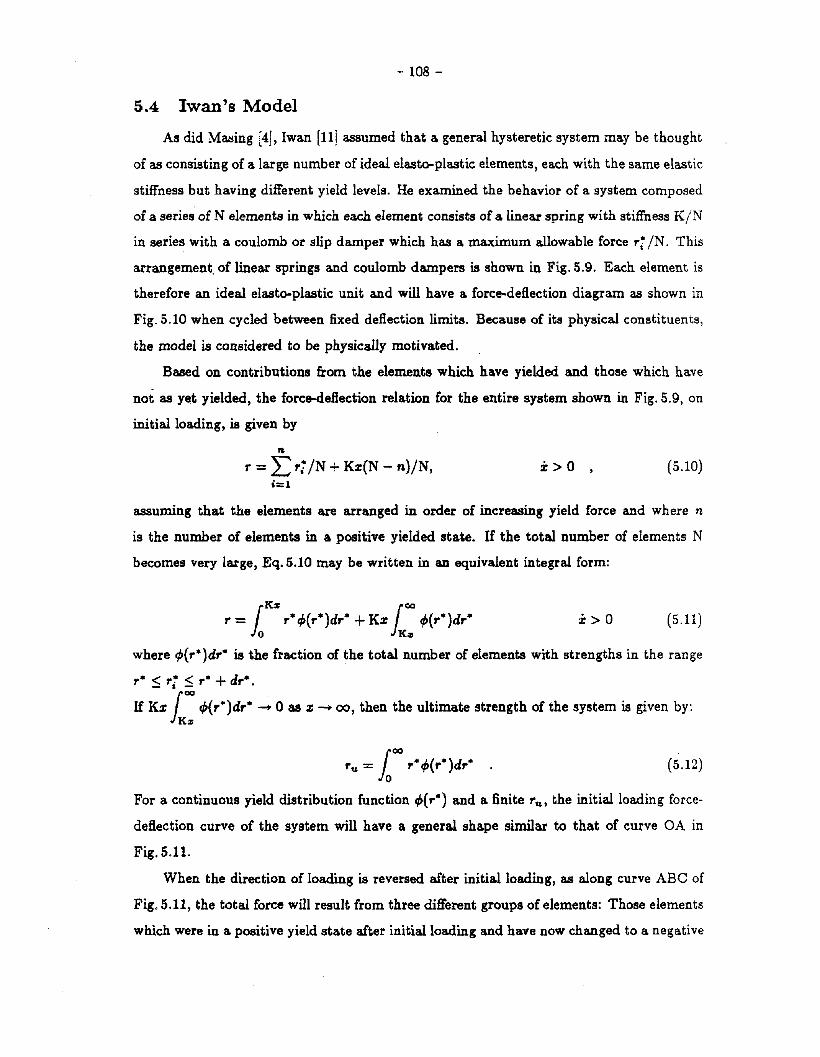
- 108 -
5.4 Iwan's Model
As did M~ing [4], Iwan [11] assumed that a general hysteretic system may be thought
of as consisting of a large number of ideal elasto-plastic elements, each with the same elastic
stiffness but having different yield levels. He examined the behavior of a system composed
of a series of N elements in which each element consists of a linear spring with stiffness KIN
in series with a coulomb or slip damper which has a maximum allowable force ri IN. This
arrangement. of linear springs and coulomb dampers is shown in Fig.5.9. Each element is
therefore an ideal elasto-plastic unit and will have a force-deflection diagram as shown in
Fig. 5.10 when cycled between fixed deflection limits. Because of its physical constituents,
the model is considered to be physically motivated.
Based on contributions from the elements which have yielded and those which have
not as Yet yielded, the force-deflection relation for the entire system shown in Fig. 5.9, on
initial loading, is given by
"r = L r; IN + K%(N - n)/N,
i=l
z> 0 , (5.10)
assuming that the elements are arranged in order of increasing yield force and where n
is the number of elements in a positive yielded state. If the total number of elements N
becomes very large, Eq. 5.10 may be written in an equivalent integral form:
lK
2: 100r = r* 4>(r*)dr* + K% 4>(r*)dr*o K2:
x>o (5.11)
where 4>(r*)dr* is the fraction of the total number of elements with strengths in the range
r* ~ r; ~ r* + dr* .
If K% roo 4>(r*)dr* _ 0 as %_ 00, then the ultimate strength of the system is given by:lK2:
r u =100
r*4>(r*)dr* (5.12)
For a continuous yield distribution function 4>(r*) and a finite ru , the initial loading force
deflection curve of the system will have a general shape similar to that of curve OA in
Fig. 5.11.
When the direction of loading is reversed after initial loading, as along curve ABC of
Fig. 5.11, the total force will result from three different groups of elements: Those elements
which were in a positive yield state after initial loading and have now changed to a negative

- 109-
yield state; those elements which were in a positive yield state after the initial loading but
have not yet changed to a negative yield state; and those elements which were unyielded
on initial loading and are still unyielded. Thus the restoring force along the path ABC will
be given by:
lK (:r:.. -:r:)/2 lK.2l..
r = -r*¢>(r*)dr* + [K% - (K%a - r*)]¢>(r*)dr*o K(.2l.. -:r:)/2
+ K% roo ¢>(r*)dr*lK.2l..
(5.13)
In order to perform a dynamic analysis of the transient response of a yielding system,
it is necessary to be able to describe the force-displacement relation of the system for
arbitrary. loading such as cyclic loading between variable limits. Recognizing this fact,
Iwan [12] explains the manner in which the force-deflection relationship between C and D
of Fig. 5.4 can be obtained, as follows:
If the fraction of elements in any given yielded or unyielded state is known at C, one need
only determine what happens to each of these separate groups as the loading is reversed.
This will lead to an expression for the foree-displacement curve between C and D of the
form:
lK (:r:-:r:c)/2 lK(:r:.. -:r:c)/2
r = r*¢>(r*)dr* + (K% - K%c - r*)¢>(r*)dr*o K(:r:-:r:c)/2
lK~ 1~+ (K% - K%a + r*)¢>(r*)dr* + K% ¢>(r*)dr*
K(:..-sc)/2 K:..
(5.14)
The above procedure could be carried on indefinitely by keeping track of the fraction of
elements in each of the yielded or unyielded category after each reversal in the direction of
loading. In this way, the entire history of the hysteresis loops may be traced out without
introducing any additional mathematical assumptions about the manner in which the loop
curves change after each reversal of the direction of loading, which is in contrast to the situ
ation in the case of purely mathematically motivated models such as the Ramberg-Osgood
model discussed earlier. Iwan [6,11,12] considers that one of the important advantages of
the distributed-element formulation is its ready adaptability to transient loading problems;

-110 -
as in the case of steady-state loading, no additional assumptions need be made and the
physics of the model itself dictates the history dependence of the loading behavior.
A review of Iwan's model shows that Eq. 5.13, which defines the steady-state response
curve ABC of Fig.5.11 (an unloading branch curve starting from virgin loading curve),
and Eq.5.14, specifying the transient response curve CD of Fig.5.4 (a reloading branch
curve not starting from the virgin curve), can be obtained using Masing's rules. All that
is required is specification of the skeleton curve OA of Fig. 5.11 or Fig. 5.4 respectively, as
in Eq.5.11. Thus, Iwan's model falls within the general class of Masing models.
The above claims can be proved as follows: The stiffness of the entire system at
any instant is given by the stiffness contributions from those elements which have not yet
yielded. Therefore, for the virgin loading curve in Eq.5.11,
dr 100
-d =K tP(r*)dr* ~g(z)z K.2:
%>0 (5.15)
(5.16)
(5.17)
Using similar arguments, the instantaneous (or tangent) stiffness corresponding to the
steady-state response curve described by Eq.5.13 is given by:
d 1K.2:4 100
/ =K tP(r*)dr* + K tP(r*)dr*z K(.2:.. -.2:}/2 K.2:..
Therefore,
dr =K (00 tP(r*)dr* =9 (Z4 - z)dz lK(.2:4 -.2:)/2 2
It is clear that Eq.5.16 can be directly obtained from the skeleton curve of Eq.5.15 by
applying Masing's rules. Similarly, from the transient loading curve in Eq.5.14,
Therefore,
dr = K roo tP(r*)d,,* = g(~)dz lK(~-.2:c)/2 2
Again Eq. 5.11 can be deduced from the initial loading curve of Eq.5.15 by using Masing's
rules. In addition, the implementation of the Masing model is much simpler, as indicated
in Eqs.5.15-11, compared with computing the force-deformation relationship for Iwan's

- 111 -
model by keeping track of element behavior, which involves several integral terms as shown
in Eqs. 5.11, 5.13 and 5.14. It can also be shown that the fate of an interior curve leaving
a completed loop is predicted by Iwan's model to be the same as specified by Rule 2 of the
Masing model.
This confirms that Iwan's model falls within the general class of Masing models and
that prescribing the yield distribution function 4>{r*) along with K is one way of prescribing
the skeleton curve for the corresponding Masing model. This also shows that the Masing
models are in accordance with the physics of a particular class of mechanical systems,
namely those consisting of a collection of elastic springs and slip dampers in the man
ner described by Iwan. Therefore, the Masing models will not exhibit any nonphysical
properties such as the ability of self-generating energy.
An application of Iwan's model using system identification was made by Cifuentes
(32], to model the restoring force behavior of reinforced concrete structures subjected
to earthquake-type dynamic loading. He modified Iwan's model to include stiffness and
strength deterioration. This was done by assuming that all but one of the elasto-plastic el
ements in the model can break after they begin yielding at certain specified displacements,
and they do not regain their stiffness and strength afterwards, thereby causing a permanent
loss of stiffness and strength.

- 112-
5.5 Other Models
5.5.1 Pisarenko's Model
Pisarenko [22] investigated the oscillations of elastic systems allowing for dissipation
of energy in the material due to 'incomplete' elasticity. The need for such a study arose
due to the demand for higher standards in the calculation of the dynamic strength of the
components of high-speed machines such as turbines and motors. He adopted a relation
proposed by Davidenkov [23] as the fundamental relation between forces and deformations
which characterizes the very slight departure from Hooke's law for the majority of materials
used in machine construction.
The expressions for the tangent stiffnesses in a symmetrical cycle as shown in Fig. 5.12
are given by:
dr [ ( )"-1]-=K1-v zo+zdz
and
dr [ ( )"-1]dz=K1-vzo -z ,
(5.18)
for the loading and unloading paths, respectively. The following final equations of the
contour curves of the hysteresis loop were obtained by integrating Eq. 5.18 taking account
of the boundary conditions of the branches of the hysteresis loop:
r = K{ z - ~ [(zo + z)" - 2"-lZ~]} (loading)
(5.19)
Pisarenko did not specify the virgin loading curve in his report. However, it can be
shown that the above set of equations, 5.18 and 5.19, could also be obtained with an
assumed virgin loading curve of
(5.20)
or, equivalently, with a tangent stiffness relation at the virgin loading of
(5.21)
and then using Masing's rules. Equation 5.21 shows clearly that for larger displacements,
the model possesses· unstable characteristics.

-113 -
5.5.2 Rosenblueth and Herrera's Model
Rosenblueth and Herrera [24J attempted to establish mildly nonlinear load
deformation, or stress-strain curves, for structures and materials with purely hysteretic
damping, so that the model gives an equivalent degree of viscous damping which is in
dependent of amplitude and of frequency under steady-state sinusoidal oscillations. The
equivalent viscous damping ) of the nonlinear system is defined so that the energy lost
per cycle by an equivalent linear system equals the energy lost per cycle by the nonlinear
system.
The above conditions imply that the resulting load-deformation or stress-strain rela
tionship should be
(5.22)
on virgin loading, where A, 01 are material constants and
(5.23)
In this derivation, Masing's rules are used to obtain the curves on unloading and reloading
(Fig.5.13). The model leads to a behavior very near to that of a linear viscoelastic material,
except that the equivalent damping ratio does not depend on frequency or amplitude.
According to Rosenblueth and Herrera, very accurate measurements taken in a large
triaxial machine showed that confined sands, gravels and broken rock behave in this manner
almost up to failure. However, a much wider class of materials, including granular soils, have
a different stress-strain behavior on first loading, although their unloading and reloading
curves can still be modelled satisfactorily in accordance with Masing's rules. Also, the
infinite stiffness at % =0 resulting from Eq. 5.22 is objectionable on several counts, including
the implied infinite velocity of small amplitude waves. Therefore, Eq.5.29 can only be
accepted as an idealization valid within a certain range of variables and for the calculation
of certain phenomena.
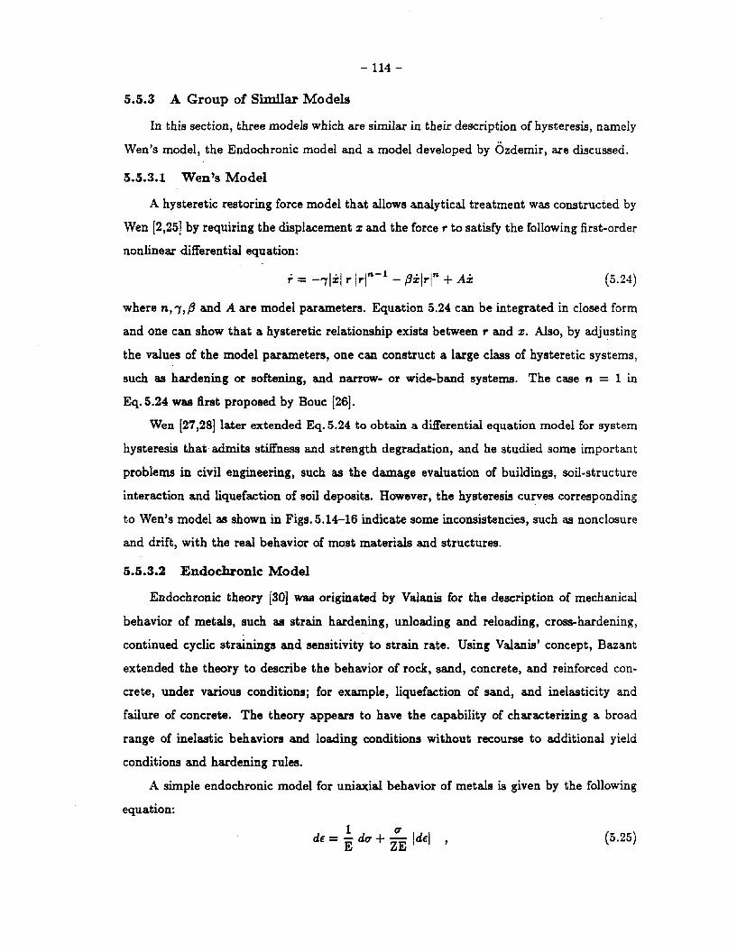
- 114-
5.5.3 A Group of Similar Models
In this section, three models which are similar in their description of hysteresis, namely
Wen's model, the Endochronic model and a model developed by Ozdemir, are discussed.
5.5.3.1 Wen's Model
A hysteretic restoring force model that allows analytical treatment was constructed by
Wen [2,251 by requiring the displacement % and the force r to satisfy the following first-order
nonlinear differential equation:
(5.24)
where n, j, f3 and A are model parameters. Equation 5.24 can be integrated in closed form
and one can show that a hysteretic relationship exists between r and %. Also, by adjusting
the values of the model parameters, one can construct a large class of hysteretic systems,
such as hardening or softening, and narrow- or wide-band systems. The case n = 1 in
Eq. 5.24 was first proposed by Bouc [26].
Wen [27,281 later extendedEq. 5.24 to obtain a differential equation model for system
hysteresis that admits stiffness and strength degradation, and he studied some important
problems in civil engineering, such as the damage evaluation of buildings, soil-structure
interaction and liquefaction of soil deposits. However, the hysteresis curves corresponding
to Wen's model as shown in Figs. 5.14-16 indicate some inconsistencies, such as nonclosure
and drift, with the real behavior of most materials and structures.
5.5.3.2 Endochronic Model
Endochronic theory [301 was originated by Valanis for the description of mechanical
behavior of metals, such as strain hardening, unloading and reloading, cross-hardening,
continued cyclic strainings and sensitivity to strain rate. Using Valanis, concept, Bazant
extended the theory to describe the behavior of rock, sand, concrete, and reinforced con
crete, under various conditions; for example, liquefaction of sand, and inelasticity and
failure of concrete. The theory appears to have the capability of characterizing a broad
range of inelastic behaviors and loading conditions without recourse to additional yield
conditions and hardening rules.
A simple endochronic model for uniaxial behavior of metals is given by the following
equation:
1 UdE = - du + - IdElE ZE
(5.25)

- 115-
where E is the elastic modulus and ZE is the limit stress of the material. This model is
rate-independent and exhibits stress-strain behavior in a manner shown in Fig. 5.17.
Sandler [31] published a very interesting paper in which he demonstrated that such
behavior violates Drucker's stability postulate and Ilyushin's postulate. Although the pos·
tulates of Drucker and Ilyushin are not strict physical or thermodynamical requirements for
the behavior of real materials, they do play an important role in the construction of rational
theories or models of material behavior for use in general dynamic problems. Through the
construction of some simple examples, he showed that the endochronic models are unsuit·
able for numerical solution of dynamical problems, for reasons such as nonunique solutions
for a physical problem with unique solution, and small errors in initial and/or boundary
conditions leading to rapid deterioration in the accuracy of the subsequent computations.
5.5.3.3 . Ozdemir'8 Model
Ozdemir's [3] objective was to obtain a mathematical model capable of describing
the force-deformation relationship for energy absorbers under gross plastic deformations
induced by random cyclic loading. He derived the following rate-independent model from
a rate-dependent model for metals:
(5.26)
A typical hysteresis loop corresponding to Ozdemir's model is shown in Fig. 5.18 which
indicates that the loops are not necessarily closed.
5.5.3.4. Conclusion
From Eqs. 5.24-26, the following can be deduced for the case X, i > 0 and r, ~ > 0 :
Wen's model:
Endochronic model:
Ozdemir's model:
(5.27)
Eq. 5.27 shows that all three models describe essentially the same hysteretic relation·
ship. The inconsistent and unrealistic characteristics discussed for each class of models
are therefore shared by all the models described by anyone of the differential equations
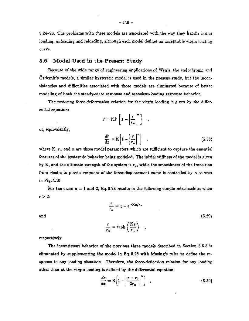
-116 -
5.24--26. The problems with these models are associated with the way they handle initial
loading, unloading and reloading, although each model defines an acceptable virgin loading
curve.
5.6 Model Used in the Present Study
Because of the wide range of engineering applications of Wen's, the endochronic and
Ozdemir's models, a similar hysteretic model is used in the present study, but the incon
sistencies and difficulties associated with those models are eliminated because of better
modeling of both the steady-state response and transient-loading response behavior.
The restoring force-deformation relation for the virgin loading is given by the differ
ential equation:
or, equivalently,
(5.28)
where K, r u and n are three model parameters which are sufficient to capture the essential
features of the hysteretic behavior being modeled. The initial stiffness of the model is given
by K, and the ultimate strength of the system is rUJ while the smoothness of the transition
from elastic to plastic response of the force-displacement curve is controlled by n as seen
in Fig. 5.19.
For the cases n =1 and 2, Eq.5.28 results in the following simple relationships when
r> 0:
and
r (KZ)- =tanh -ru r u
(5.29)
respectively.
The inconsistent behavior of the previous three models described in Section 5.5.3 is
eliminated by supplementing the model in Eq. 5.28 with Masing's rules to define the re
sponse to any loading situation. Therefore, the force-deflection relation for any loading
other than at the virgin loading is defined by the differential equation:
dr =K[l-I~I"]dz 2ru(5.30)

- 117-
where ro is the restoring force at the point of load reversal chosen according to Rules 1
and 2.
The relation above is simple and practical, and yet is general enough to be useful as
a model for the dynamic, hysteretic behavior of a wide range of softening materials and
structures. As shown in Figs. 5.20 and 5.21, the hysteresis loops for the model introduced
are closed and exhibit no drift. An important feature of a model is our ability to select
its parameters in a manner that is physically meaningful. This objective is easily achieved
with the present formulation, since two of the parameters, namely K and ru , are the initial
stiffness and the ultimate strength of the system under investigation. This means, for
example, that these parameters could be determined during structural design from material
properties and the plans of a structure. Application of this model in system identification
of .hysteretic structures is discussed in the next chapter.

-118 -
REFERENCES
[1] Jennings, P.C., "Periodic Response of a General Yielding Structure," Journal of theEngineering Mechanics Division, ASCE, Vol. 90(2), 131-166, April, 1964.
(21 Wen, Y.-K., "Method for Random Vibration of Hysteretic Systems," Journal of theEngineering Mechanics Division, ASCE, Vol. 102(2), 249-263, April, 1976.
[3] Ozdemir, H., "Nonlinear Transient Dynamic Analysis of Yielding Structures," Ph.D.Dissertation, Division of Structural Engineering and Structural Mechanics, Department of Civil Engineering, University of California, Berkeley, California, June, 1976.
(4] Masing, G., "Eigenspannungen und Verfestigung beim Messing," Proceedings of the2nd International Congress for Applied Mechanics, Zurich, Switzerland, 332-335, 1926.(German)
[5] Scott, R.F., Foundation Analysu, Prentice-Hall, Inc., Englewood Cliffs, New Jersey,1981.
(6] Iwari, W.O., "On a Class of Models for the Yielding Behavior of Continous and Composite Systems," Journal 01 Applied Mechanics, ASME, Vol. 34(3),612-617, September, 1967.
(71 Mr6z, Z., "On the Description of Anisotropic Workhardening," Journal 01 the Mechanics and Physics 01 Solids, Vol. 15, 163-175, 1967.
(8] Prevost, J.-H., Abdel-Ghaffar, A.M. and Elgamal, A.-W.M. "Nonlinear HystereticDynamic Response of Soil Systems," Journal 01 Engineering Mechanics, ASCE, Vol.111(5), 696-713, May, 1985.
[9] Prevost, J.-H., Abdel-Ghaffar, A.M. and Lacy, S.J., "Nonlinear Dynamic Analyses ofan Earth Dam," Journal 01 Geotechnical Engineering, ASCE, Vol. 111(7), 882-897,July, 1985.
[10] Elgamal, A.-W.M., Abdel-Ghaffar, A.M. and Prevost, J.-H., "Elasto-Plastic Earthquake Shear-Response of One-Dimensional Earth Dam Models," Earthquake Engineering and Structural Dynamics, Vol. 13, 617-633, 1985.
[11] Iwan, W.O., "A Distributed-Element Model for Hysteresis and Its Steady-State Dynamic Response," Journal 01 Applied Mechanics, ASME, Vol. 33(4),893-900, December, 1966.
[12] Iwan, W.O. "The Distributed-Element Concept of Hysteretic Modeling and Its Application to Transient Reponse Problems," Proceedings 01 the -lth World Conference onEarthquake Engineering, Vol. II, A-4, 45-57, Santiago, Chile, 1969.
[13] Jennings, P.C., "Earthquake Response of a Yielding Structure," Journal 01 the Engineering Mechanics Division, ASCE, Vol. 91(4),41-68, August, 1965.
[14] Jennings, P.C., "Response of Simple Yielding Structures to Earthquake Excitation,"Ph.D. Dissertation, California Institute of Technology, Pasadena, California, June,1963.

-119 -
[15] Matzen, V.C. and McNiven, H.D., "Investigation of the Inelastic Characteristics of aSingle Story Steel Structure using System Identification and Shaking Table Experiments," Report No. EERC 76-20, Earthquake Engineering Research Center, University of California, Berkeley, California, August, 1976.
[16] Fan, W.R.-S., "The Damping Properties and the Earthquake Response Spectrum ofSteel Frames," Ph.D. Dissertation, University of Michigan, 1968.
[17] Tanabashi, R. and Kaneta, K., "On the Relation Between the Restoring Force Characteristics of Structures and the Pattern of Earthquake Ground Motions," Proceedings01 the Japan National Symposium on Earthquake Engineering, Tokyo, Japan, 57-62,1962.
[18] Herrera, 1., "Modelos Din8.micos para Materiales y Estructuras del Tipo Masing," Bol.Soc. Me~. Ing. Sism., Vol. 3(1), 1-8, 1965. (Spanish)
[19J Newmark, N.M. and Rosenblueth, E., Fundamentau 01 Earthquake Engineering, Prentice Hall, Inc., Englewood Cliffs, New Jersey, 1971.
[20] Ramberg, W. and Osgood, W.R.; "Description of Stress-Strain Curves by Three Parameters," Technical Note No. 902, National Advisory Committee on Aeronautics,July, 1943.
[21J Ang, A.H., "Analysis of Frame with Non-Linear Behavior," Journal 01 the EngineeringMechanics Division, ASCE, Vol. 86(3),1-24, June, 1960.
[22j Pisarenko, G.S., "Vibrations of Elastic Systems Taking Account of Energy Dissipationin the Material," Technical Documentary Report No. WADD TR 60-582, February,1962.
[23J Davidenkov, N.N., "On Energy Dissipation in Vibrations," Journal 01 TechnicalPhysics, Vol. VIII(6), 483, 1938. (Russian)
[24J Rosenblueth, E. and Herrera, I., "On a Kind of Hysteretic Damping," Journal 01 theEngineering Mechanics Division, ASCE, Vol. 90(4),37-48, August, 1964.
[25] Wen, Y.-K., "Equivalent Linearization for Hysteretic Systems Under Random Excitation," Journal 01 Applied Mechanics, ASME, Vol. 47(1), 150-154, March, 1980.
[26j Bouc, R., "Forced Vibration of Mechanical Systems with Hysteresis," Abstract,Proceedings 01 the ith Conference on Nonlinear Oscillation, Prague, Czechoslovakia, 1967.
[27J Baber, T.T. and Wen, Y.-K., "Random Vibration of Hysteretic Degrading Systems,"Journal of the Engineering Mechanics Division, ASeE, Vol. 107(6), 1069-1087, December, 1981.
[28j Wen, Y.-K., "Stochastic Response and Damage Analysis ofInelastic Structures," Probabilistic Engineering Mechanics, Vol. 1(1), 49-57, 1986.
[29] Spencer, Jr., B.F. and Bergman, L.A. "On the Reliability of a Simple Hysteretic System," Journal 01 Engineering Mechanics, Vol. 111(12), 1502-1514, December, 1985.

-120 -
[30] Chen, W.-F., and Ting, E.C., "Constitutive Models for Concrete Structures," Journalof the Engineering Mechanics Division, ASCE, Vol. 106(1), 1-19, February, 1980.
[31] Sandler, 1.S., "On the Uniqueness and Stability of Endochronic Theories of MaterialBehavior," Journal of Applied Mechanics, ASME, Vol. 45(2), 263-266, June, 1978.
[32] Cifuentes, A.a., "System Identification of Hysteretic Structures," Report No. EERL84-04, Earthquake Engineering Research Laboratory, California Institute of Technology, Pasadena, California, 1984.

- 121 -
r
x
Fig. 5.1 Force-Deformation Curve of a Masing Element
r
Fig. 5.2 Hysteretic Loop for Cyclic Loading

rj
_•
u..,
A
]0
..: 1'1 "
I\ ~
;.,I'I
,-,
,:'
10'
II
Jl:
II
I.,
XII,
,1
'-•
.RII
!'-
I
..,1"
"\',
,II l,jl
,,,,
'I;
I ......
B(-
Xo
.-ro
l8
t>;l
t>;l I
(i
1IN
ITIA
LL
Y(i
i)LO
AD
ED
(iii)
LOA
DE
D(i
v)U
NLO
AD
ED
ISO
TR
OP
ICT
OP
TOA
TO
8
(a)
(b
)
Fig
.5.3
(a)
Mas
ing
Hys
tere
sis
Loo
pan
d(b
)M
ult
iple
'Sti
ffne
ss'
Sur
face
s

- 123-
r
x
Fig. 5.4 Hysteretic Loop for Transient Loading

- 124-
...0....
.~w
a.I-tn
~llQC.00~
"':' .!l.f llQ
CII- ...CII
\() ....en... >... ::coZ -;;
E ....=u CIIu ed 'C- CII~ c.en ><'0 ~
~~
bb'"
....i ~
e
L..------I. ~-----~I.:_-----..J~N 0 "t "1
i~df)l) ;J I_~ ... O..=

- 125-
LINEAR ,x~ ..J~,~ COULOMB ~_
FRICTION
Fig.5.6 Physical Interpretation of a Single Masing Element
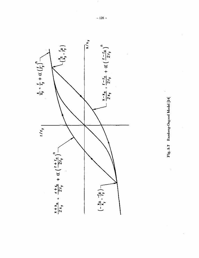
(_
'1..0
-ro
)x. y
•ry
x+
Xo
::
2x'
yr+
ro+
ex:(
r+
r0)n
2r y
2r y
rfry
.!..
_r
(rn
xy
-T
+ex:
r)y
y
(Xo
.!':2)
xy•
ry
X/x
. y
nx
-xo
=r-
ro+
ex:(r-ro
)2
xy
2r y
2ry
~ t-.:l
(J) I
Fig
.5.7
Ram
berg
-Osg
ood
Mod
ell1
4j

- 127-
2.52.01.5
~& '12.
0.5o
1.5r----~--_r_--_r_--_r--__.,
0.5 r---~""""~:::-:t----l----+-----1
1.0
x Ix'!
Fig.5.8 Skeleton Curves Obtained via Ramberg-Osgood Relation [3J
KIN KIN' .•. KIN'" . KIN
*r· INI
rFig.5.9 Iwan's Model for a General Hysteretic System [11J
r.I
A
Fig.5.l0 Force-Displacement Relation of Each Elasto-Plastic Element in Fig. 5.9

- 128r
A
c
Fig. 5.11 Hysteresis Loop for Iwan's Model
r
x
Fig.5.12 Hysteresis Loop for the Model Studied by Pisarenko [22)
r
Fig. 5.13 Hysteresis Loop for Rosenblueth and Herrera's Model [24]

- 129-
Fig. 5.14 Hysteretic Forces Corresponding to Random Displacements for Wen's Model[21
r
Fig.5.15 Typical Force-Displacement Curves for Wen's Hysteretic Oscillator Subjectedto White Noise Acceleration at Base [29}
400. OC ,------,.----r----r-----,
200.00
....u<rct...
~ 0.001--------4--------1-<rc
~ -20C. oc ~I
-.00. 0st.'""'o::----_"""".·.'="0---0"...-=0,...----:-.'""'.o:-----="e. CDISPLRCEMENT
Fig.5.16 Drifting Characteristic of Wen's Model
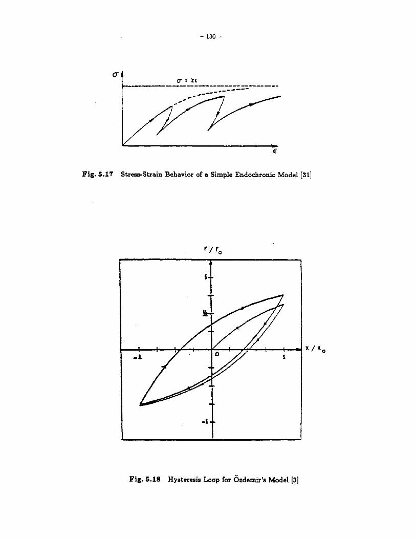
- 130-
(j:%t
~----------------------------------------..------------, ......
Fig.5.1T Stress-Strain Behavior of a Simple Endochronic Model [31]
Fig. 5.18 Hysteresis Loop for Ozdemir's Model [3]

- 131 -
400.00
K =150.0
ru =200.0
300. 00
UJUtI:0LL
~ 200.00 n =00z l.....tI:0I-(f)
UJtI:
100. 00
II I I
2.0 3.0 4.0DISPLACEMENT
Fig.5.19 Effect of n on the Force-Displacement Curve of Eq. 5.28
40 O. 00 ,....----r----,..----~-----,
200.00
u..;uct:cu..c.:J C.OOz-a:c~
Vlwa::
··200.00
-40 C. O.~ 1..:.O::-----.-;"4~.O:::-----:::C.l....::::-0------;4J-.':::"O--~8.C
DISPLACEMENT
Fig.5.20 Hysteresis Loop for Periodic Response of the Model in Eqs. 5.28 and 5.30

- 132-
.00. 00 ~--........,----.....----.------.
200.00
&oJUa::c
""t.:l 0.00Z
a::c~
en&oJa::
-200.00
40C. 019....O~---,~..."O,.----.O,.l-. ..,..O--.....,.,L.,.o,.--~e. Q
.00.00 ------,-----,..----.-----.
200.00
&oJ
'"'a::C
""t.:l C.OOz-a::c~
en&oJa::
-200.00
-'CC. 0J9L.,.0..-----'.,......,,0,........---..,,0,1-."""C----,.',.I...:o,...------="e. c
.00.00....------,----.....----.------.
200.00
&oJUa::c""t.:l C.OCz-a::c~
en&oJa::
-200.0C
400. OSeL..0"..---_.".l•...,0,...-----.0,.l-. ..,..0---,l..,.o""--~e. 0
DISPLFlCE"ENT
Fig.5.21 Force-Displacement Curves for Arbitrary Loading of the Model in Eqs. 5.28 and5.30
- 133 -
CHAPTER 6
SYSTEM IDENTIFICATION APPLIED TO THE INELASTIC
PSEUDO-DYNAMIC TEST DATA
6.1 Introduction
In this chapter, it is shown how the restoring force-deformation relationship for a multi
degree-of-freedom structure excited by earthquake accelerations can be described using the
new hysteretic model. For simplicity, the structure is then idealized as a shear building with
the hysteretic model relating the story shears and story drifts. In particular, the pseudo
dynamic test structure, described in Chapter 2, which is a full-scale six-story steel-frame
building, is modeled in this fashion, and methods are then given to estimate analytically
the structural parameters involved in the modeling, such as the small-amplitude elastic
stiff'nesses and strengths of stories.
A hysteretic system identification program, HYSID, is developed to determine the
optimal estimates of the hysteretic model parameters from experimental data. The op
timization algorithm involves continual alternating between the steepest descent and the
modified Gauss-Newton methods for the simultaneous identification of the optimal param
eter values in a (3N + I)-dimensional space where N is the number of degerees-of-freedom
in the structure. This program is used to obtain the optimal estimates of 18 model pa
rameters, resulting from the hysteretic modeling of the six-story test structure, by using
the inelastic pseudo-dynamic test data. The prior estimates of the structural parameters
described in the previous paragraph &reused as the starting values for HYSID.
The prediction capability of the model obtained from the inelastic pseudo
dynamic test data is tested by subjecting it to the ground motion from the small-amplitude
elastic pseudo-dynamic test and then comparing the model responses predicted with the
measured structural responses. Conclusions are given concerning the prospects of using the
hysteretic model in seismic analysis of structures.

- 134 -
6.2 Application of the Hysteretic Model to a Full-Scale Six-Story
Steel Structure
6.2.1 Simplified Structural Model
The equation of motion of the N-story building in Fig.2.1 can be written as:
Mi + R = - Mi(t) 1"..." """-# """"J )
(6.1)
where!! is the vector of restoring forces at each degree of freedom. The restoring force
Ri at the degree of freedom i stems from the interaction of that degree of freedom with
all other degrees of freedom and with the ground. Therefore, the following relationship is
assumed:N
Ri =2: RijJ=O;*1
(6.2)
in which ~j (j 1: 0) is the restoring force exerted at degree-of-freedom i by degree-of-freedom
j due to the relative motion between the two, and ~o is similar except it represents the
interaction with the ground.
Rij is hysteretic and depends on the history of relative displacement (Xi - Xj), so R jj
is written in the following functional form:
R·· - I·· (x· - x·)IJ-IJ 1 J' j =0, 1, 2, ... , N j j 1: i , (6.3)
where Xo = O. The functionals lij are symmetric, i.e., lij (x) = fji(x), and odd, l.e.,
lij (-x) = -lij (x), so Rji = -Rij.
This model can be compared with the linear elastic case for which
where Kij is the elastic stiffness of the spring between degrees of freedom i and j.
For the present hysteretic model which was introduced in Chapter 5, the virgin loading
is given by the following nonlinear differential equation relating ~j and (Xi - Xj):
(6.5)
where Kij is the initial stiffness, ru, ij is the ultimate strength and nij is a model parameter,
associated with the degrees-of-freedom i and j. The Masing model can be used to obtain
any unloading and reloading branch curve.

- 135 -
6.2.1.1 Shear Building Approximation
By introducing do shear building approximation, it is assumed that the shear resistance to
any degree of freedom comes only from its adjacent degrees of freedom,
From Eq.6.2,
i.e., Rij == 0 If i, j 3 Ii - j I > 1 (6.6)
Ri == Ri, i-I + Rot, i+1 (6.7)
With the introduction of story shears as shown in Fig.6.1 in which Ri,i-l == rj,
Ri,i+ 1 = - ri+ I , Eq. 6.7 becomes:
Equation 6.5 can be used to relate the story shear forces and story drifts in Fig.6.1,
according to which,
(6.9)
(6.10)
In the above hysteretic relationships, Ki and Ki+l are the initial stiffnesses, ru • i and ru • i+l
are the ultimate strengths, and ni and ni+l are model parameters, of stories i and i+1,
respectively. This shear building approximation will be used in the modeling of the pseudo
dynamic test structure described in the following section.
6.2.2 Structural DetaUa of Test Building
As described in Section 2.5, a six-story, two-bay structure which would represent a
portion of a complete building was adopted for the full-scale test. The Boor plan of the
test structure is shown in Fig. 2.7 and the elevations of the exterior and interior frames in
Fig. 2'.8. The material and structural properties of the members used are shown in Table
6.1, while the member sizes are presented in Figs. 6.2 and 6.3.
6.2.2.1 The Eccentrically-Braced Frame
Two of the most common structural systems used to resist seismically-induced forces
a.re the moment-resisting frame and the concentrically-braced frame. However, a moment
resisting frame may not have enough elastic stiffness to control strong drift and nonstruc
tural damage under service loads and minor earthquakes. The concentrically-braced frame

- 136-
has excellent lateral elastic stiffness properties to control story drift and resist minor ground
shaking, but the braces can repeatedly buckle under compressive cyclic loading and so can
suffer a drastic decrease in their buckling strength and their ability to dissipate energy [2).
The eccentrically-braced frame has both the properties of high elastic lateral stiffness
and good energy-dissipation capacity. By offsetting the braces a distance e as in Fig.6.3,
a link is formed between braces framing into a common girder. The performance of an
eccentrically-braced frame during a major earthquake depends largely on the inelastic be
havior of the links. In a well-designed eccentrically-braced frame, except for the plastic
hinges at the ground level column bases, all the inelastic activity of the frame should be
concentrated in the links. Also, the braces in the eccentric-bracing system can be designed
not to buckle before the formation of active links in the girders, which is difficult to guar
antee for concentrically-braced frames [2}. In the following section, a classification of active
links is presented.
6.2.2.2 Active Links
The following classification has been developed [3,4} with reference to the behavior of
active links, which strongly depends on their length. If they are sufficiently long, plastic
moment hinges form at both ends of the links. On the other hand, if these links are short
they tend to yield in shear with smaller end moments. The shear-moment interaction
diagram shown in Fig. 6.4 can be used to illustrate the difference between the two kinds of
active link behavior. The relevant parameters in reference to Fig. 6.5 are defined as follows:
The plastic moment capacity is:
(6.11)
in which the effect of shear is neglected, and 111 = yield stress of steel, and Z = plastic
section modulus.
The plastic moment capacity reduced due to shear is:
M; =1y (bJ - tw ) tJ (d - tJ )
assuming that the web is in a plastic state and carries shear only.
The plastic shear capacity is:
(6.12)
(6.13)

- 137-
assuming that the web is yielding in shear and using the von Mises yield criterion.
At the balance point shown in Fig. 6.4, M; and V; are reached simultaneously. Then
for the equilibrium of the link in Fig. 6.6 which is at the balance point,
* 2Mp *e =-V *p
(6.14)
By comparing the actual lengths of links with e* , the following conclusions can be reached:
(i) Active links whose lengths are equal to or shorter than e* will yield predominantly in
shear and are called shear links;
(ii) Links that are longer have moment-shear interaction;
(iii) The end moments of such long links will approach the plastic moment capacity Mp ,
and moment hinges will form at the ends of the links. These links are referred to as
moment links.
Experimental results indicate that shear link action continues to predominate for
lengths up to approximately 1.15e* [5]. Also, it has been observed that shear links are
more effective energy dissipators than moment links, although in frames shear links are
likely to be subjected to larger ductility demands than longer moment links [3].
The analysis presented in this section is used later in this chapter to classify the links
in the eccentrically-braced pseudo-dynamic test structure.
6.2.3 Prior Estimation of Structural Parameters
6.2.3.1 Story Stiffnesses by the First-Mode Approximation Method
In the first-mode approximation method (FMA) [6,7], the story stifFnesses for the
shear-building model are calculated using known characteristics of the first mode, such as
the fundamental frequency and the first-mode shape, of the structure being modeled. The
modal properties may be from experiments in the case of an existing structure, or from a
more detailed finite element model of the structure.
The modal equations of the shear-building model can be expressed as follows:
K ?(r) =w; M ?(r),..,. ,..,. (6.15)
where K is the stiffness matrix of the shear building, M is the diagonal mass matrix, W r is
the natural frequency of the rth mode, and ?(r) is the rth modeshape vector. Corresponding,..,.to the first mode, Eq.6.15 becomes:
K?(1) =w~ M?(l),..,. ,..,. (6.16)

- 138 -
For the test structure und~r consideration which is modeled as a six-story shear build
ing, Eq. 6.16 could be expanded as follows:
o
o
(6.17)
Equation 6.17 is now rearranged to give:
116~1)ooooo
I16P) - 116~1)
-4>~1) + 4>~1)
oooo
o.J.(1) .J.(1)0/2 - 0/3
-4>&1) + 116&1)ooo
oo
.J.(1) .J.(1)0/3 - 0/"
-4>~1) + 4>~1)
oo
ooo
.J.(I) .J.( 1)0/" - 0/5
-4>~1) + 4>~1)
o
oooo
.J.( 1) ",,(I)0/5 - 0/6
_¢J~I) + ep~l)
K1
K2
*K3
K"KsKe
ml 4>~1)
m2 4>~1)
= W; ~ 4>~I)(6.18)
~ 4>11
)
Ins 4>~1)
me 4>~I)
In the above formulation, mi represents the mass associated with the ith degree-of-freedom,
whereas 4>~1) is the component of the first mode at the ith degree-of-freedom.
The first-mode characteristics, as identified from the elastic pseudo-dynamic test data,
are given in Table 4.1 of Chapter 4:
WI = 11.370 raJ1j8, and
4>(1) = [0.295, 0.531, 0.778,1.012,1.222, 1.403]T .,...
- 139 -
The mass ma.trix is taken to be the one given by Boutros and Gael [8/. Using these
quantities, the system of linear equations (Eq.6.18) can be solved for the story stiffnesses
K1 , K oz , ••• , K6 • The calculated story stiffnesses are given in Table 6.2, and their variation
with story level is plotted in Fig. 6.7 where the stiffnesses are marked at the mid-points of
the stories.
With the knowledge of the story stiffnesses, the stiffness matrix K of the shear building
is constructed as in Eq.6.17. Equation 6.15 is then solved for the natural frequencies and
modeshapes corresponding to this stiffness matrix resulting from the first-mode approxi
mation method. The calculated natural periods are given in Table 6.3 and the modeshapes
are plotted in Fig. 6.8.
6.2.3.2 Story Stifl'neBBeB Using Biggs' Formula
An approximate formula for the initial stiffness of a story in a multi-story frame, used
by Anagnostopoulos [9J and reportedly from Biggs, is employed in this section. The stiffness
of a particular story is estimated by making the following assumptions:
(a) column shears above and below a joint are equal\
(b) inflection points in columns above and below a joint are located symmetrically;
(c) rotation of all joints in a floor are equal.
With these assumptions aad using slope-deflection equations, the following equation for the
story stiffness was obtained:
(6.19)
where
E = modulus of Elasticity,
h - story height,
I = beam length,
I - moment of Inertia,
2: Kc - L: (l/h) for all columns in the story,
2: Kga == L:(I/l} for all beams in the floor above, a.nd
2: Kgb= L:(l/l) for all beams in the floor below.
For braced frames one could use [9]:
(6.20)

- 140 -
where K/ r is the story stiffness of the corresponding unbraced frame which is computed
from Eq. 6.19, and Kbr is the contribution by the braces to the story stiffness which is given
by
where
~ AE 2Kbr = L- -1- cos a , (6.21 )
A= area of bracing,
1 = length of bracing,
a = angle between bracing and beam, and
lJ= summation over all the braces working in tension.
However, the braces of the test structure in the present study have been designed to
resist both tension and compression, and in this eccentric bracing system the braces are not
to bucld~ before the shear yielding of active links (1\. Hence, for the stiffness calculations
following, the summation in Eq.6.21 is taken over all the braces working in tension and
also in compression.
Frames A and C of the test structure are unbraced moment-resisting frames with one
column in each oriented for weak-axis bending, and their story stiffnesses are calculated
using Eq.6.19. Frame B of the test structure is also a moment-resisting frame, and in
addition, it has eccentric K-bracings in its north bay. The story stiffnesses of frame Bare
calculated using Eqs.6.19-21. The story stiffnesses of the test structure are then given by
the sum of the story stiffnesses of all three frames A, B and C.
Stiffnesses of all the stories of the test structure are calculated in the above manner,
and the results are presented in Table 6.2 and Fig. 6.7. With the knowledge of these
story stiffnesses, the stiffness matrix K of the shear building is constructed as in Eq.6.17.
Equation 6.15 is then solved for the natural frequencies and modeshapes corresponding
to this stiffness matrix resulting from Biggs' formula. The calculated natural periods are
given in Table 6.3 and the modeshapes are plotted in Fig.6.8.
6.2.3.3 Comparison of the First-Mode Approximation Method and
Biggs' Formula
The initial story stiffnesses of the test structure have been estimated by the first-mode
approximation method and also by using the Biggs' formula. The modal characteristics
resulting from these approximations have also been computed.

- 141 -
Approximate values for the story stiffnesses are also measured directly from the hys
teresis loops, obtained from the inelastic pseudo-dynamic test, which are shown in Fig. 6.9.
Stiffness values from all three methods are now compared in Table 6.2 and Fig.6.7. From
Fig. 6.7, it is clearly seen that the first-mode approximation method gives rise to stiffnesses
which are very close to the stiffness values measured directly from the test hysteresis loops.
The Biggs' formula results in estimates of the story stiffnesses which are much too large
except for the first story, confirming the observation of Lai and Vanmarcke [7]. This is not
surprising since Anagnostopoulos [9] has already suggested that Biggs' formula for braced
frames would not be as accurate as the formula for unbraced frames. It should be noted,
though, that the Biggs' formula gives a purely theoretical result whereas the first-mode
approximation method as used here utilized results derived from the structural tests.
The natural periods and modeshapes resulting from the first-mode approximation
method and the Biggs' formula are compared in Table 6.3 and Fig. 6.8, respectively, along
with the results from the system identification method applied to the 'elastic' pseudo
dynamic test data using the multiple-input multiple-output technique. In calculating the
story stiffnesses by the first-mode approximation method, the shear building was assumed
to have the same first-mode characteristics as that of the test structure estimated by the sys
tem identification method. Therefore, for this mode, the first-mode approximation method
agrees exactly with the system identification results. However, for the other modes, it seems
that Biggs' formula results in a slightly better comparison with the dystem identification
results than the first-mode approximation method.
In summary, the first-mode approximation method results in better stifffness prediction
though only the first-mode characteristics are reproduced well, while Biggs' formula does
better with the higher modes. If the properties of the first mode can be estimated by
reliable means such as experiments or detailed elastic finite element analyses, then it would
be better to choose the first-mode approximation method to calculate story stiffnesses.
6.2.3.4. Estimation of Story Strengths
The strength of each story in the test structure is estimated by assuming that this
story has been transformed into a mechanism. As shown in the following, the strength
of each frame in the test structure is calculated separately, and the strengths of all three
frames are then added in order to estimate the story strength.

- 142 -
(i) Plastic Moment Capacities of Columns and Girders
The plastic moment capacities of columns and the negative moment capacities of gird
ers are calculated using the following equation:
(6.22)
where
1,,= yield stress of ASTM A36 steel, and
Z = plastic section modulus of steel member.
As mentioned above, only the negative moment capacities of composite girders C l.n be
calculated using Eq.6.22 since slab concrete cracks in tension.
(ii) Plastic Positive Moment Capacity of Composite Girders
The positive moment capacities of girders are calculated by taking into account the
composite action of steel girder and concrete slab [2,101.
(a) Effective Width of Composite Steel-Concrete Girders:
The effective width of concrete flange bE (Fig. 6.10) is determined according to AISC:
1.11.1.
(b) Positive Moment Capacity
The procedure for determining the ultimate moment capacity depends on whether the
neutral axis occurs within the concrete slab or within the steel girder. If the neutral axis
occurs within the slab, the slab is said to be adequate, Le., the slab is capable of resisting
the total compressive force. If the neutral axis falls within the steel girder, the slab is
considered inadequate, Le., the slab is able to resist only a portion of the compressive
force, the remainder being taken by the steel girder. In the following, full composite action
is assumed, and also since any longitudinal reinforcement within the effective slab width
usually makes little difference to the strength of a composite section, it is neglected.
• Case I-Slab Adequate
From Fig. 6.11, the ultimate compressive force
and the ultimate tensile force
c = 0.85/~ bE IJ (6.23)
(6.24)
- 143 -
Equating C and T for equilibrium .gives
(6.25).,-
According to AISC: 1.11.5.2-1, a from Eq.6.25 has to satisfy the following:
(6.26)
where t c is the concrete slab thickness above the steel deck.
The neutral axis distance % is calculated from
(6.27)
where IiI is given by ACI: 10.2.7.3.
Full yield capacity of the steel girder is achieved when
% < t, and(6.28)
where
(t, - %)
E, =0.003 :-
and
~ _ Iv~v--
Elleel
Then the ultimate positive moment capacity M~ becomes
M~ =TI = IvA, (~ + t, - i)
(6.29)
(6.30)
• Case 2-Slab Inadequate
If the depth 11 aa determined in Eq.6.25 exceeds the thickness t c of the slab above
the deck, the stress distribution will be aa shown in Fig. 6.12, assuming the steel section
a.ccomodates plastic strain in both tension and compression at ultimate strength, i.e., a
compact section.
The ultimate compressive force Cc in the slab is
(6.31)
- 144-
The compressive force in the steel girder resulting from the portion of the girder above the
neutral axis is shown in Fig. 6.12 as C3 •
The ultimate tensile force T satisfies
For equilibrium,
T = Cc +C.
From Eqs.6.32 and 6.33,
Assuming that the neutral axis is within the flange thickness of the girder,
from which S can be calculated for the case S 5 t,.To determine h:
The distances 11 and 12 in Fig. 6.12 are given by
S11 = d - h - - and
2t c
12 = d + t. - h - 2"
The ultimate positive moment capacity M;t for Case 2 is
(iii) Capacity of Shear Links
(6.32)
(6.33)
(6.34)
(6.35)
(6.36)
(6.37)
(6.38)
Equations in Section 6.2.2.2 can be used to show that the portions of the girders
between braces in the eccentrically K-braced frame B act as shear links. The shear capacity
of these shear links, V;, can be calcula.ted using Eq.6.13.
(iv) Behavior of Braces
At the ultimate capacity of a shear link, the shear force acting on that link is V;
then the maximum force acting on the brace will be
(6.39)
- 145 -
where a is the angle between the brace and the girder.
The brace force~ corresponding to its yielding and buckling can be calculated, respectively,
fromp y = !y,br Abr andp _ 1l'2EIbr (6.40)
e - L2
An effective column length factor of 1.0 [1] has been assumed in the calculation of the
critical buckling load Pe in Eq.6.40.
For all braces in the test structure, it can be shown that
(6.41)
Le., the braces neither yield nor buckle before the yielding of links in shear.
(v) Collapse Loads of Frames A, B and C
The story strength of each frame is calculated by applying the principle of virtual work
to the corresponding story collapse mechanisms shown in Figs. 6.13 and 6.14. Wand M's
in these figures are the story collapse load and the plastic moment capacities of members,
respectively.
According to the principle of virtual work,
External Work = Internal Strain Energy . (6.42)
• Frame A (C)
For the collapse mechanism of frame A(C) in Fig. 6.13, the virtual work principle gives
(6.43)
• Frame B
Similarly for frame B in Fig. 6.14,
L9 +; = -; gives
e

- 146-
(6.44)
Once the story collapse loads of frames are calculated using Eqs. 6.43 and 6.44, the strength
of the test structure is obtained by summing the collapse loads of all three frames at each
story level. The results are shown in Table 6.4.
6.2.4 Optimal Estimation of Structural Parameters by System Identification
6.2.4.1 Hysteretic System Identification Technique, HYSID
An output-error approach for system identification called HYSID is used in conjunction
with the steepest-descent and modified Gauss-Newton methods to determine the optimal
estimates of the parameters for the hysteretic model from experimental data.
• Output-Error Method
The output-error e , defined in Eq. 3.1, is gi~en by:,..",
(6.45)
where each component is the output-error in the floor displacements, velocities, accelera
tions, relative to the ground, and story shears, respectively.
The model parameters are:
(6.46)
where N is the number of degrees of freedom in the structure, and Ki , ru,i and ni are the
story parameters described in Section 6.2.1.1.
The optimal values for the model parameters are calculated by minimizing a measure
of-fit J(i) which is obtained using the definition in Eq.3.2 and the output-error ~ in Eq.
6.45:
where the normalizing quantities are such that, (6.47)

- 147 -
(6.48)
• Optimization Algorithm
To determine the optimal estimates for the 3N model parameters which minimize
the measure-of-fit J(t) in Eq.6.47, a combination of the steepest-descent method and the
modified Gauss-Newton method [11] is chosen because of its simplicity and computational
efficiency over other gradient methods.
Steepest Descent Method:
The method of steepest descent is defined by the iterative algorithm
VJC!;)b+l =b - Pic lI VJ(b)1I1
h · . a! .... J (tJ VJ <he) ) In d fr hwere Pic IS a nonnegative sc ar nunuIUzmg ;!.Jc - P II VJ (b)Ill' wor s, om t e
point he we search along the direction of the negative gradient {-VJ (b)} to a minimum
point on this line; this minimum point is taken to be !bc+l'
Modified Gauss-Newton Method:
The measure-of-fit JCV is approximated locally by a quadratic function and this ap
proximate function is minimized exactly. Ifhe is the k-th estimate for the model parameters,
J can be approximated by the truncated Taylor series near he as:
(6.49)
Then, J (!) is minimized at
(6.50)
If J(iJ is twice continuously differentiable, then the algorithm is well-defined near the
optima! estimates l since the Hessian matrix VVJ(iJ is positive definite. But for estimates
remote from!, this is not so, and the algorithm must be modified in order to guarantee
convergence.
Since J is not quadratic in! (Eqs.6.9, 6.47), a stepsize P > 0 is introduced to ensure
that the value of J decreases at every iteration step. For both the steepest descent and the
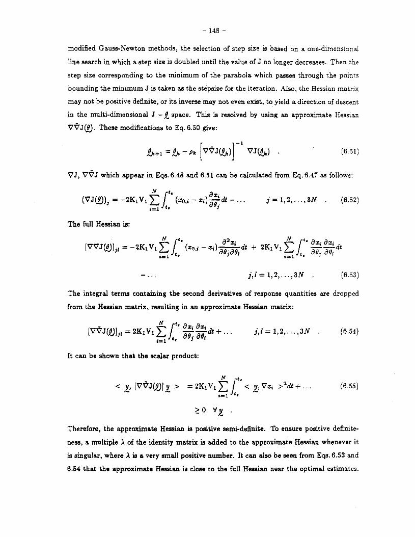
- 148 -
modified Gauss-Newton methods, the selection of step size is based on a one-dimensional
line search in which a step size is doubled until the value of J no longer decreases. Then the
step size corresponding to the minimum of the parabola which passes through the points
bounding the minimum J is taken as the stepsize for the iteration. Also, the Hessian matrix
may not be positive definite, or its inverse may not even exist, to yield a direction of descent
in the multi-dimensional J - 1... space. This is resolved by using an approximate Hessian
'VVJ(O. These modifications to Eq.6.50 give:
(6.51)
'VJ, 'VVJ which appear in Eqs.6.48 and 6.51 can be calculated from Eq. 6.41 as follows:
The full Hessian is:
j= 1,2, ... ,3/i . (6.52)
j,1=1,2, ... ,3/i (6.53)
The integral terms containing the second derivatives of response quantities are dropped
from the Hessian matrix, resulting in an approximate Hessian matrix:
It can be shown that the scalar product:
j,1=1,2, ... ,3N . (6.54)
< y, ('VVJ(!J] y >--- ---
(6.55)
2:0 V" .---
Therefore, the approximate Hessian is positive semi-definite. To ensure positive definite
ness, a multiple Aof the identity matrix is added to the approximate Hessian whenever it
is singular, where A is a very small positive Dumber. It can also be seen from Eqs.6.53 and
6.54 that the approximate Hessian is close to the full Hessian near the optimal estimates.

- 149-
In Eqs.6.52-55, only the terms corresponding to the displacement output-error are shown
for brevity.
The model responses and the sensitivity coefficients which appear in the expressions for
J, Y'J and Y'VJ are calculated from the equation of motion of the structure together with
the hysteretic relationship for the model using a fourth-order Runge-Kutta method. Figure
6.15 illustrates the process of parameter estimation in a very simplified Bow diagram.
6.2.4.2 Analysis of Pseudo-Dynamic Inelastic Test Data
The pseudo-dynamic test structure was 'excited' by the Taft 821 W a.cceierogram of the
1952 Kern County, California earthquake, scaled to a peak acceleration of 50% g (Fig. 6.16),
to study the inelastic behavior of steel-frame structures during strong ground motions.
This inelastic test data is analyzed using the hysteretic system identification technique,
HY8ID, described in the previous section, in order to determine the optimal estimates of
the structural parameters which then enable prediction of the structural responses to other
ground motions. In this study, the story shears are chosen for matching (Le., Ki == 0, i ==
1,2,3 and K" = 1, in Eq.6.41) because of their significance in hysteretic modeling and the
unique availability of measured shear forces due to the nature of the pseudo-dynamic test.
The identification results are presented below.
• Identification Results
The hysteretic system identification program HYSID, described in the previous section,
is used to estimate the optimal values of the structural parameters from the Phase II
inelastic pseudo-dynamic test data. Several runs of the program HYSID were conducted,
each with a different set of starting values for the model parameters, which are explained
in Table 6.5. The value of measure-of·fit J at the begining of each run is also given in
Tabie 6.5. The results of this investigation are presented in Table 6.6. The mean values of
the optimal estimates from all nine runs are also calculated in Table 6.6. These optimal
estimates of story stiffnesses, story strengths and n values are plotted in Fig.6.18 along
with their respective mean values to examine the reliability of the identified parameter
values from different runa.
It should be expected that all the runs result in the same optimal estimates for the
parameters. However, Fig. 6.18 shows that the parameters are not identified uniquely. This
could be due to any presence of interaction between parameters which can result in a fairly
flat region containing all the minimum points.

- 150-
In spite of the diversity of the initial starting estimates for the different runs of ijYSID
as can be seen in Table 6.5, the optimal estimates are close in all cases, except for the
story strengths of the top three stories which show a large scatter about their mean values
in Fig. 6.18. This was expected because the structure did not experience any significant
inelastic deformation at the top three stories (Fig.6.9), and hence the determination of
story strengths from these data is an ill-conditioned process since large changes in ru make
only small changes in the response. It is clear that a story strength cannot be estimated
with any confidence if the story is not exercised well into its inelastic regime.
The mean values of the stiffnesses and strengths in Fig. 6.18 exhibit a decreasing trend
with height, as expected, except for a lower first-story stiffness because of its greater height;
n takes values around 2.0. However, the fifth-story stiffness, strength of the fourth story
and n values for stories 4 and 5 appear anomalous. The strength and n may be interacting
because of the insignificant inelastic deformation of the top three stories during the test;
the high stiffness of the fifth story is more likely due to the effect of the feedback errors
during the pseudo-dynamic test, which is neglected in the analysis.
The stiffness matrix of the shear-building model whose story stiffnesses are the optimal
estimates of stiffnesses of each case in Table 6.6, is calculated using Eq.6.17 and then
Eq.6.15 is solved for the natural periods and modeshapes. The results are given in Table
6.7 and Fig.6.19, respectively. Comparing Tables 6.3 and 6.7, it can be seen that the
shear-building assumption in FMA and HYSID which made use of experimental results,
causes the estimate for the third-mode period to be too high (0.13-0.14 sec) compared
with the MI-MO result (of 0.10 sec) which is not based on such a model. The modest
increase in the periods of the first two modes from HYSID compared to MI-MO may be
the result of deterioration which causes period elongation. The interesting result is that
the above modal characteristics for all the runs of HYSID are extremely close. For this
reason, and also neglecting any small scatter of the optimal estimates about their mean
values in Fig.6.18, the mean values of the optimal estimates in Table 6.6 will be used for
any further investigation.
The time-histories of the optimal model responses at the roof level, mid-height and at
floor 2 are compared with the test results in Fig.6.20. The model predictions are excellent
which is in agreement with the small values of measure-of-fit J in Table 6.6. Hysteresis
curves obtained from the pseudo-dynamic test are compared with the curves 'predicted' by

- 151 -
the optimal hysteretic model in Fig. 6.21. The hysteresis predictions are also very good.
A measure of the maximum amount of inelastic deformation each story has experienced
during the test is defined by the 'fraction of inelasticity' as follows:
Fr t · fIn 1 .. Maximum Story Shearac Ion 0 e astlClty = ------.:...--
Story Strength(6.56)
This fraction of inelasticity predicted by the optimal hysteretic model is calculated for each
story of the test structure using the values of maximum story shear predicted by the model
and the optimal estimates of the story strength, and the results are given in Table 6.8.
These results suggest that the inelastic deformation experienced by the first three stories
during the test should have been much larger compared to the top three stories which is
indeed true as seen from the test hysteresis loops in Fig. 6.9. Also, that the fraction is close
to unity in the first three stories demonstrates a strong nonlinear behavior and indicates
that a linear model would have performed poorly.
6.3 Seismic Analysis of Structures Using the Hysteretic Model
The prediction capability of the hysteretic model is examined in this section in order
to support the use of the model in seismic analysis of structures. It would be nice to test
the optimal model discussed in the previous section using an independent inelastic test
of the six-story structure. However, the only other pseudo-dynamic test data available
to the author was the 'elastic' case where the test structure was subjected to the Taft
S21W accelerogram with a scaled peak value of 6.5% g. These test data were therefore
compared with the response calculated using the optimal model parameters identified from
the pseudo-dynamic inelastic test data. The model responses predicted are compared with
the measured elastic test data at the roof in Fig. 6.22. The time-histories of responses agree
well over the duration of the test. The responses may have agreed even better if feedback
errors were accounted for, as in Chapter 4, when model response was calculated.
In addition, it also has to be noted that the optimal estimates of the model parameters,
in general, do not differ very much from their prior estimates (Table 6.9) and therefore the
latter also should give reasonably good response predictions. This is supported by the
small J-value of only 9% corresponding to the prior estimates. From Table 6.9, a value
of 2 for the model parameter n seems reasonable for steel-frame structures, taking into
account any possible interaction between the parameters of the fourth and fifth stories.

- 152 -
This corresponds to the following force-deformation relationship on virgin loading:
r (KX)- = tanh -ru r u
(6.57)
It is planned to use the hysteretic model with other available earthquake data to esti
mate possible values of the model parameter n for different materials and structures. Thus,
the hysteretic model could be used in the seismic analysis of structures using structural pa
rameters estimated from the preliminary structural plans, thereby facilitating at the design
stage an effective and iterative process to control structural responses to ground motions.
- 153 -
REFERENCES
[1] Askar, G., Lee, S.J. and Lu, L.-W., "Design Studies of the Six Story Steel Test Building:U.S.-Japan Cooperative Earthquake Research Program," Report No. 467.3, FritzEngineering Laboratory, Lehigh University, Bethlehem, Pennsylvania, June, 1983.
[2] Rides, J .M. and Popov, E.P., "Cyclic Behavior of Composite Floor Systems in Eccentrically Braced Frames," Proceedings 01 the 6th Joint Technical Coordinating Committee Meeting, U.S.-Japan Cooperative Research Program Utilizing Large-Scale TestingFacilities, Maui, Hawaii, June, 1985.
[3j Popov, E.P. and Malley, J.O., "Design of Links and Beam-to-Column Connectionsfor Eccentrically Braced Steel Frames," Report No. UCB/EERC-83/03, EarthquakeEngineering Research Center, University of California, Berkeley, California, January,1983.
[4] Neal, B.G., "Effect of Shear Force on the Fully Plastic Moment of an I-Beam," Journal01 Mechanical Engineering Science, Vol. 3(3), 258, 1961.
[5] Malley, J.O. and Popov, E.P., "Shear Links in Eccentrically Braced Frames," Journal01 Structural Engineering, ASCE, Vol. 110(9), 2275-2295, September, 1984.
[6j Nielsen, N.N., "Dynamic Response of Multistory Buildings," Ph.D. Dissertation, California Institute of Technology, Pasadena, California, June, 1964.
[7] Lai, S.-S.P. and Vanmarcke, E.H. "Overall Safety Assessment of Multistory Steel Buildings Subjected to Earthquake Loads," Publication No. R80-26, Department of CivilEngineering, Massachusetts Institute of Technology, Cambridge, Massachusetts, June,1980.
[8] Boutros, M.K. and Goel, S.C., "Pre-Test Analysis of the Six-Story Eccentric-BracedSteel Test Building," Proceedings 01 the 5th Joint Technical Coordinating CommitteeMeeting, U.S.-Japan Cooperative Research Program Utilizing Large-Scale TestingFacilities, Tsukuba, Japan, February, 1984.
[9j Anagnostopoulos, S.A., Roesset, J .M. and Biggs, J .M., "Non-Linear Dynamic Response and Ductility Requirements of Building Structures Subjected to Earthquakes,"Publication No. R72-54, Department of Civil Engineering, Massachusetts Institute ofTechnology, Cambridge, Massachusetts, September, 1972.
[10] Salmon, C.G. and Johnson, J.E., Steel Structures: Design and Behavior, Harper &Row, Publishers, Inc., New York, 1980.
[11] Luenberger, D.G., Introduction to Linear and Nonlinear Programming, Addison-WesleyPublishing Co., Massachusetts, 1973.

- 154-
Member Property
Girders, Floor Beams and Columns Wide-flange shapes made of ASTM A36 Steel
Braces Rectangular tubes of ASTM A500 Grade B Steel
Slabs 3! - lightweight concrete, approximate dry
weight = 105 pd, fc = 3000 psi
Decking 3- QL-99-16
Studs r (190)
Table 6.1 Structural Properties of Members in the Test Structure [11
Elastic StUfneu (tom'/em)
StoryTest HY8teresis :FMA Method Bigg8' :Formula
1 184.7 199.4 189.9
2 236.3 233.9 291.8
3 200.0 198.5 286.8
4 161.8 170.8 284.7
5 130.6 134.2 238.1
6 89.4 77.2 237.6
Table 6.2 Elastic Story Stift'nesses Estimated by Different Methods
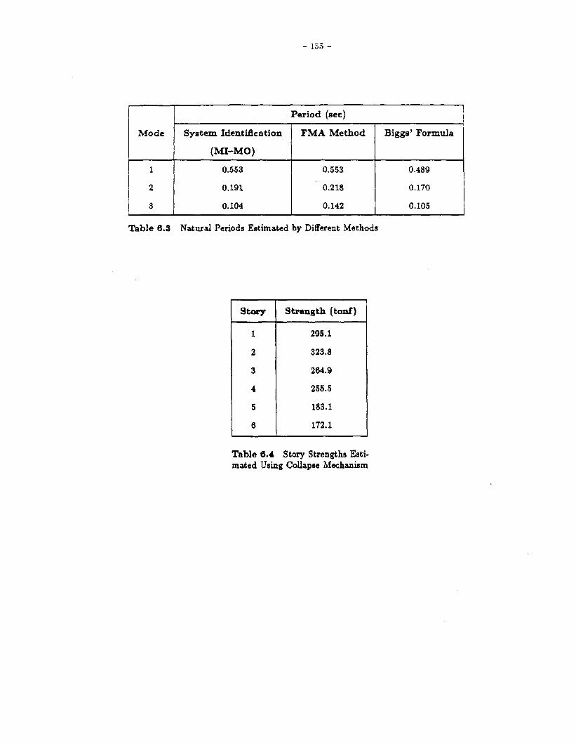
- 155 -
Period (sec)
Mode System Identification FMA Method Biggs' Formula
(MI-MO)
1 0.553 0.553 0.489
2 0.191 0.218 0.170
3 0.104 0.142 0.105
Table 6.3 Natural Periods Estimated by Different Methods
Story Strength (toni)
1 295.1
2 323.8
3 264.9
4 255.5
5 183.1
6 172.1
Table 6.4 Story Strengths Estimated Using Collapse Mechanism

- 156 -
Case Initial Estimate of! (Eq.6.46) Initial J (%)
1 K for each story: prior estimates using the test
hysteresis loops (Ta.ble 6.2)
r u for each story: prior estimates using collapse
mechanism (Table 6.4) 9.1
n for each story = 1.8: gives minimum value to the
measure-of-fit J (Fig. 6.17) in which
K and r to used are the above prior
estimates.
2 10% smaller than in Case 1 43.7 II
3 10% larger than in Case 1 65.9
4 +10%, -10%, +10%, -10%, ... larger than in Case 1 9.0I
5 K, r u : 15% larger than in Case 156.0
n : 15% smaller than in Caae 1
6 K, r u : 15% smaller than in Caae 1!
54.9 I
n : 15% larger than in Case 1 !
7 +20%, -20%, +20%, -20%, ... larger than in Case 1 8.5
8 25% smaller than in Caae 1 106.7
9 25% larger than in Caae 1 152.1
Table 6.5 Different Runa of the Program HYSID to Estimate the Optimal Values of theStructural Parameters from the Phase n Inelastic Teat Data

Op
tim
al
Est
imate
sS
tory
Para
mete
rc
•••
Mean
Val
ue
12
a4
I)6
18
9
K18
8.0
190.
118
3.0
194.
319
0.4
189.
420
1.0
192.
119
5.1
191.
5
1f u
317.
231
4.8
318.
132
2.8
319.
331
6.1
324.
631
4.3
315.
431
8.1
n1.
61.
61.
61.
51.
61.
61.
41.
61.
71.
6
K21
4.4
215.
621
6.3
210.
321
6.5
214.
720
4.0
212.
621
4.9
213.
3
2f u
279.
827
9.2
283.
327
3.5
280.
227
8.2
266.
627
4.0
282.
327
7.5
n1.
71.
71.
71.
91.
71.
72.
21.
81.
71.
8
K17
2.2
171.
917
5.4
169.
216
8.9
172.
517
1.9
174.
416
9.6
171.
8
3f u
252.
424
8.7
256.
125
7.8
251.
525
2.6
279.
925
4.3
265.
425
7.6
n2.
32.
32.
32.
32.
52.
31.
82.
12.
02.
2
K15
5.9
153.
216
0.0
154.
915
5.9
154.
315
1.2
147.
714
4.6
153.
1
4f u
353.
934
6.5
350.
531
5.5
376.
833
0.7
291.
336
2.3
412.
534
8.9
n3.
13.
12.
93.
43.
03.
23.
43.
23.
43.
2
K25
7.8
254.
025
6.5
267.
226
8.8
251.
725
1.5
233.
923
9.5
253.
4
5f u
201.
419
0.9
183.
027
1.3
222.
219
8.9
288.
521
0.7
228.
322
1.7
n1.
01.
11.
20.
70.
81.
20.
91.
41.
41.
1
K10
9.8
109.
810
2.9
113.
711
6.1
106.
611
0.1
125.
410
4.7
111.
0
6f u
175.
116
9.4
197.
914
3.4
214.
714
9.2
135.
681
.022
1.0
165.
3
n1.
91.
82.
22.
01.
72.
22.
21.
92.
52.
0
J(%
)4.
04.
14.
14.
04.
04.
04.
04.
04.
04.
0
Tab
le6
.6O
pti
mal
Est
imat
esof
Stf
uct
ura
lP
aram
eter
sfr
omth
eD
iffe
rent
Run
sof
HY
SID
.... 01~ I

- 158-
Period (sec)Case Mode
I 2 3 4 5 6
1 0.561 0.196 0.134 0.099 0.076 0.071
2 0.561 0.196 0.134 0.099 0.076 0.071
3 0.561 0.198 0.136 0.099 0.076 0.070
4 0.560 0.194 0.133 0.099 0.076 0.070
5 0.560 0.194 0.132 0.098 0.075 0.070
6 0.561 0.197 0.135 0.099 0.076 0.071
7 0.561 0.196 0.133 0.099 0.077 0.071
8 0.562 0.196 0.130 0.099 0.077 0.072
9 0.564 0.199 0.136 0.100 0.077 0.072
Table 6.'7 Comparison of Modal Periods Corresponding to the Optimal StoryStiffnesses Resulting from the Different Runs of HYSID
Story Fraction of Inelasticity,
Predicted
1 0.92
2 0.93
3 0.85
4 0.56
5 0.64
6 0.41
Table 6.8 Predicted Values for theExtent of Inelastic Deformation

- 159-
Elastic Stiffness Strength
(toni/em) (toni)n
Story
Prior Optimal Prior Optimal Prior Optimal
1 184.7 191.5 295.1 318.1 1.8 1.6
2 236.3 213.3 323.8 277.5 1.8 1.8
3 200.0 171.8 264.9 257.6 1.8 2.2
4 161.8 153.1 255.5 348.9 1.8 3.2
5 130.6 253.4 183.1 221.7 1.8 1.1
6 89.4 111.0 172.1 165.3 1.8 2.0
Table 6.9 Comparison of the Prior and Optimal·Estimates of the StructuralParameters

- 160-
I
Xi+1I ;---ri+4 - J
Xi ---~
ri - IXi-4 ----
I
STORY i +1
STORY
,, ,,
Fig. 6.1 Illustration of Story Shear Forces and Story Drifts
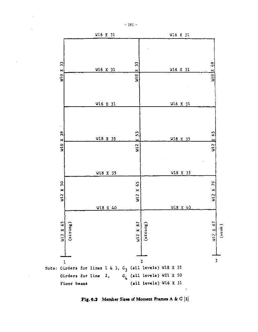
W16 X 31
- 161 -
W16 X 31
'"" .., a-'"" ..,
~
>= W16 X 31 >= W16 X 31 x0 0 0... ... ...3 3 3
W16 X 31 W16 X 31
a- M &r\
'"" &r\ -.0
>< W18 X 35 ..... w18 X 35 ~
0 N N.... .... ...3 3 3
W18 X 35 W18 X 3S
0 &r\ a-&r\ -.0 ">< >< X
N N N.... .... ...3 3 3
W18 X 40 ~-l18 X 40
<l'\ - " ..... "-.0 00 co 00 coc c
>= 0 >= 0 Xl-o l-o
N U N U N.... en ... :1.1 -3 '-" 3 '-" 3
- _I....- --1 2 3
Note: Girders for lines 1 & 3, G3 (all levels) W18 X 3S
Girders for line 2, G4(all leve ls) w21 X SO
Floor beams (all levels) Wl6 X 31
Fig. 6.2 Member Sizes of Moment Frames A .k C [11

- 162 -
o.....3
wI8 X 35
oW16 X 31 ~ W16 X 31
><I-------------~~-----.....,.:....:::..r;:..:..----~o~
3
Wl6 X 31
0\0
W18 X 35>< x0 ('of..... 03
..... .....3 3
W18 X 40 W18 X 40
CJ'\\0
l'0 CJ'\~ l'
>< >< XN ('of.....3
.....3
w18 X 40
\0 \00..... C"'l.....'>< ><N N.....3
~
3
1 2 3
Fig.6.3 Member Sizes of Braced Frame B with Eccentric Braces [11

- 163 -
v
BALANCE POINT
V •p t----.--.
M
FIg.6." Typical Shear-Moment Interaction Diagram for Wide Flange Sections [3]
1 bJ-f----4
d
Fig.6.5 Girder Dimenaions
FIg. 6.6 An Active Link at the Balance Point

- 164-
2 0 TEST HYSTERESISLOOPS
X F"'A METHOD
<> BIGGS' FORMULA
?I
II
~\
\ ,
\I
II
+I
\I»I /
//I '
6
.-J4UJ>UJ.-J
>-a:: 3o....en
o 100 200 300
STORY STIFFNESS (tont/em)
400
Fig.6.1 Variation of Stiffness with Story Level Estimated by Different Methods

oS
YS
TE
MID
EN
TIF
ICA
TIO
N(M
I-M
O)
aF
MA
ME
TH
OD
()B
IGG
S'
FO
RM
UL
A
......
0>
CJ.
,,/)~
//~'
/,
/,./l
\" \
'x~,
'""
'""~
'i
,-,.
1("_..
../'
\//
"
I•
I I ~ I I I , I .,. I I I I I. "
356 ..
RO
Of
fLO
OR
2
FU
ND
AM
EN
TA
LM
OD
ES
EC
ON
DM
OD
ET
HIR
DM
OD
E
Fig
.6.8
Mo
dca
hap
caO
bta
ined
byD
iffe
rent
Met
ho
ds

20
0.
CO
."."~
,l-~
TOR
YS
20
0.0
0
i '"t: IeO
.CO
cr '"Z II>
~ Ie '" :;;-2
00
.00
-1._
n'
...,.oJ
I---L.~_._
__
2.0
O.C
2.0
f.0
5101
11O
RIF
I1(
111
O.
00~
--IF
.II
-tO
O.
OJ,
'0-2
'0
O~0
2:
0(.
0
S101
11O
Rlf
l1(
111
TE
S
40
0.
00lU
ii
I
20
0.0
0
ST
OR
Y2
z e .... «: '" :;;-2
00
.00
Ie cr ... Z II>
0.0
0I
Jff
·00
.0
0Iiii
I
-tO
O.
01\L
-,
IlU
T-
.0-2
.00
.02'
CI
5111
Rl
Oll
lFl
1(1
11
'•.
C
.TO
RY
I
~ Ie '" :;;-2
00
.00
z '"~ Ie cr ... Z II>
.00
.00
II
I'
.TO
RY
4I
.OL
W.
II
II
TO
RY
54
00
.00
1iii
i
.lO
ftY
&
..... 0>
0> I
TE
ST
-tO
O.O!\~-~-----to----ro-----.
c51
0111
OR
I.l
1(11
1
20
0.0
0
z '"t: ~ Ie '" :;;-2
00
.00
I0
.00
1.I
-I'"Z II
>
f.O
TES
T
20
0.0
0
z e !''"r
--7\
I
:;;-2
00
.0
0~
I-t
OO
.COl
-'-_
~._'_
-t.O
-2.0
0.0
2.0
51
0R
lO
RIF
I1
(lIl
-2'
CI
TE
ST
o.0
_-"-~
--'1
5lap
~01
1"1
2.0
__
----
1•
1(l
Ilf.
O-t
OO
.0_
1\.
C
~ Ie '" :;;-2
00
.00
~0
.00
r-I----
z II>z e
20
0.
CO
Fig
.6.9
Hy
ster
esis
Loo
psfr
omth
eIn
elas
tic
Pse
ud
o-D
yn
amic
Tes
t

- 167 -
bE~---_--..:=.-------·I
-----------------------~--------------------- Its (AISC: 1.11.5.1-5)
.,
Fig.6.10 Composite Steel-Concrete Section

~------------~------------I
V//////
1/////,1
'1
/ / / / / / ~ / / / / /V
//////
1//////1
~~-
r-,L c
r
bE
(j)
Com
posi
'eS
ectio
n
--1
'5 d
0.00
3
~_I~
=-1.
=-IC~~----:-
~'I d
(ii)
Ult
ima
teS
tra
in
c L
T
'y
(iii)
Ult
ima
teS
tre
ss
..... 0>
00 I
Flg
.6.1
1S
tres
san
dS
trai
nD
istr
ibut
ions
atU
ltim
ate
Mo
men
tC
apac
ity
for
Cas
e1
-S
lab
Ade
quat
e
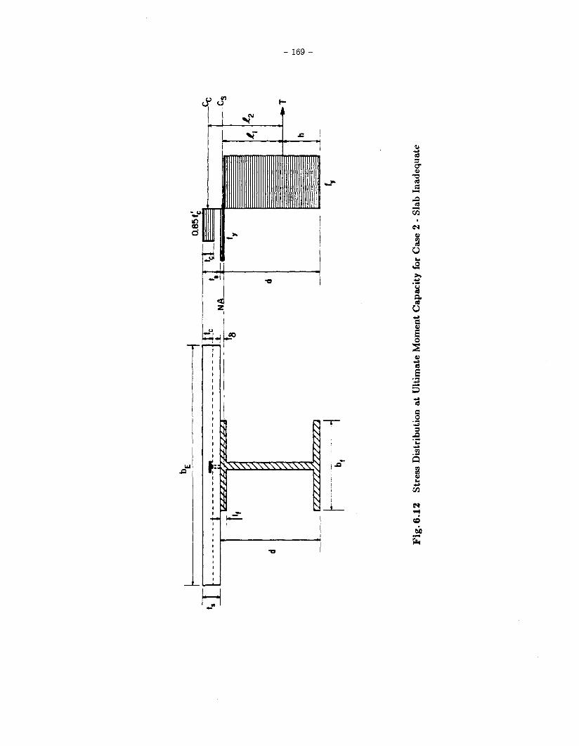
O.85
f~
,Cc
t~,
t·Cs
f rI
I
T.....
.C
ll coh
1--
--i-
''1
d
-~~------bf
d
IbE
.1
'~[_h_---rrm
__-"!!'
-_--h
--------
-If"-..
"L977~"'---
-----
---rc
-1t t
8
Fig
.6.1
2S
tres
sD
istr
ibut
ion
atU
ltim
ate
Mom
ent
Cap
acit
yfo
rC
ase
2-
Sla
bIn
adeq
uate

i
iIih
- 170 -
h
wIIIIIIIIIIII
~ ~ J
Fig. 6.13 Story Collapse Mechanism for Frame A(C)
LI. ~
r - - - - - - - - - - - ±----,..--t' - - - - JI 'I , fI I I , I
I I \ II I I 'II I,' \ II I I \ II I I , II I I , II I I \ I
I Ms ' " , I M: ~ '# 6W-""~------:~+";;;"J'It;"-+~+--......::~--,--
M, M4
-------~-----~---------~---I ,I \
I ,
I \I \
I \I ,
I ,
I ,
I \
I" "Ic ~----------~
Fig. 6.1~ Story Collapse Mechanism for Frame B
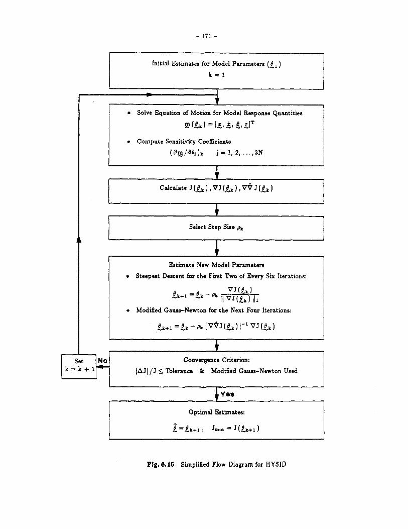
- 171 -
Initial Estimates for Model Parameters (!1 )
k=1
I
t• Solve Equation of Motion for Model Rellponse Quantities
m(!t) = [.!o, ~, £, LIT
• Compute Sensitivity Coefficients
(am/a8j )t j = 1,2, ... ,3N
tCalculate J C!k ) , VJ C!t ) , VV J C!t )
tSelect Step Sin Pk
~
+Estimate New Model Parameters
• Steepest Descent for the First Two of Every Six Iterations:
_ VJ (!t)!t+l-!t -Pt II VJ(!k) III
• Modified Gauss-Newton for the Next Four Iterations:
!k+1 =!t - Pt [VVJ (!t) r l VJ (!t)
+Set No Convergence Criterion:
k=k+l .... I~JI / J ~ Tolerance & Modified Gauss-Newton Used
tVe•
Optimal Estimates:
!=!t+l' Jmia = J C!k+1)
Pig.8.15 Simplified Flow Diagram for HYSID

60
0.
40
0.
-
..--. u UJ
(/) ""u
20
0.
-U
J(/) ""L U Z
O.
~0
\~~[Vi
H t- «
I
cr UJ
-20
0.
-
\IW
11
-J
.... --l
UJ
t,;)
U u «
-40
0.
-
-60
0.
0.0
r--
2.5
r 5.0
J-----r--~--r----·
7.5
10
.01
2.5
15
.0T
IME
(SE
C)
-r1
7.5
20
.0
Fig
.6
.16
Taf
t82
1W
Acc
eler
ogra
m,
1952
Ker
nC
ou
nty
,C
alif
orui
a,B
arth
qu
ake
(pea
kH
cale
dto
50%
g)

2.0
0
1.7
5
(n=
1.8
1J m
in=
9.1
%)
0.5
0
0.2
5
1.5
0J t-
1.2
5H u.. I u.. 0 I
1.0
0IJ
J a: ::l
Ul
I\
/I
......
ct--
-lCA
l
IJJ
0.7
5~
0.0
0
o.1
.2
.3
.4
.5
.
n6
.7
.8
.9
.1
0.
Fig
.6.1
1S
elec
tion
of
Init
ial
Est
imat
efo
rn

- 174 -
II'll
~------'ll
'll
•••~e
100.0
I s 4 I
8tory
100.0...-----------------------------,
II400.0
•
------_'!.• "•
Ii
III
I-~~------~
Il.. IIl I
I" I
II
• •
• •'II.
•••
•~-----
•
100.0
100.0
0.0 l...- .....L --l.. ..l-. .l- '-- -'
I s I I
Story
. ...~--......
• IILO
1.0
4.0...-----------------------------,I
I
.... ·1.....; ....;-.....-1
••"..-.--'----•• •
n 1.0
I sStory
4 •
Fig.6.18 Plots of Optimal Estimates and the Mean Values of Structural Parameters

MO
D£
J
~
MO
DE
2M
OD
E'
RO
OF
MO
DE
'..
00
£~
MO
D£
6
..... -I "" I
Fig
.6
.19
Co
mp
aris
on
of
Mo
des
hap
esC
orr
esp
on
din
gto
the
Op
tim
alS
tory
Sti
ffnc
sses
Res
ulti
ngfr
omth
eD
iffe
rent
Ru
ns
of
IIY
SID

10
.0
-7.5
I
-10
.0
0.0
2.5
I5
.0
---l
----
------
T
7.5
10
.0T
IME
(SE
C)
r---
1
2.5
I1
5.0
17
.5
Fig
.6.2
0(a
)C
ompa
riso
nof
Roo
fD
ispl
acem
ents(-
Inel
asti
c}'
:;eu
do-D
Yli
amic
Tc:
;t;
--
-O
pti
mal
Hys
tere
tic
Mod
el)

- 177-
100 . ....,...----------------------------.,
50.
UUJen"-%~ O.
>I-.....Ua...Jw -50.>
-100.
-125.
o. 1. 2. 3. 4. 5.TIME (SEC)
6. 7. 8. 9.
100.
75. -
50. -~ A A
}U 25. - A ! ~wen ,"-% -
~ ~~ o.
> ~I- -25. -.....~u
\a...Jw -50. ->
~
-75. - V
-100. -
-125. I I I I I T T T9. 10. 11. 12. 13. 14. 15. 16. 17. 18.
TIME (SEC)
Fig. 6.20(b) Comparison of Roof Velocities (- lnelaatic Pseudo-Dynamic Test;- - - Optimal Hysteretic Model)

- 178 -750.
500.
u...en.....~ 250.en.....Z~
o.z~...ca:~ -250 ....(,J(,Jc
-500.
-750.o. 1. 2. 3. 4. 5. 6.
1000.
750.
U 500.~.....(,J
~ 250.z~
o.13......~ -250 ........J...~ -500.
-750.
12.8.7.6.
+----r-----r----r---"TI------,-j----9. 10. 11.
-1000.
1000.
750.
E 500.en.....(,J
~ 250.z!:!
o.~...~ -250 .......J...(,J
~ -500.
-750.
18.15.TIME (SECl
14.13.12.
+----r-----,----r----TI----r----I16. 17.
-1000.
Fig.6.20(c) Comparison of Accelerations at Floor -4 (-Inelastic Pseudo-Dynamic Test;- - - Optimal Hysteretic Model)
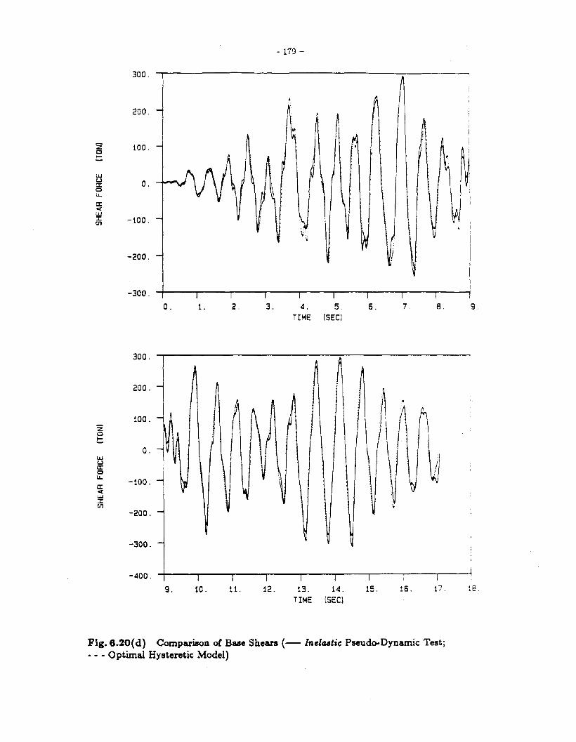
- 179-
300.
I200. l ill
I
Z 100.0::
lJJu O.a:
~0u..a:«lJJ:J: -100.U1
V·.'\
-200.
-300.
o. 2. 3. 4. 5.TIME (SEC)
6. 7. 8. 9.
300.
200.
~
100.Z0
::o.
lJJU Ia:0u..
-100.a:«lJJ:J:U1
-200.
-300.
-400.
9. 10. U. 12. 13. 14. 15. 16. 17 18.
TIME (SEC)
Fig.6.20(d) Comparison or Base Shears (- Inelutic Pseudo-Dynamic Test;. - . Optimal Hysteretic Model)

- 180 -
MODEl.'
,uIST~Y I
200. 00 r
a:c
· -,," .. r
-.00.0.9.''-,.0,-----"'2..."0--...,u""".,,..u--~;;....,.0""---"". C
STORT DRIFT
z
"Ii o.oo>.------..,p.,t.~
in
400. CO .--,----,.---.,..-------.,ISTORY I
i
20C. 00 lI
c. 00 I
::: ::..,1'''---::_':f2:'00---;o;l-I?;'"0--"'\"2"'~o,.-_T£_S_T~tSTeRT ORIn 10K)
zc
400.00 i
I ,.... f ISTORY 2
~
ST~Y2
I20C.00 200. 00 1
i I i !c 0
o.J!
0.00 I a:, , c:
" ~I I /
I q
J:<
-200. 00 l-200.00r I0
'" i
I I( I I MODEL:
-400.0_'1&: 0 i -.OO.O~iC-2. C O. C 2. C (',0 -~ ... r.. c :to C " r
STORT DRIFT ICKI STORT OR IF T {CM,
.00. 00 ,
I400.00I
ISTORY:3 ii
ST~Y3
I I200. 00 ~ '""""I J
iI i I
c i 0iI I
a: o co I '" 0.00a: • !
Ia:
~~
in ;;;
I
:<"
mj0
'" -200.00 '" -200.00
MODELI !
-400.0.9.: 0, -.00. D.p.'. 0
-2. ;) C.O 2'. C •. 0 ..". c 6. C 2. \.: ,. C
STORT ORIFT lCK' STORr ORIFT {O'l
Fig. 6.21 Comparison of Hysteresis Behavior from the Inelastic Pseudo-Dynamic Testand the Optimal Hysteretic Model

- 181 -
'00 00l I
ISTORY 4
I,200. 00 ii Ic
Ir O. cc'" I~
'" I I~ I
j
ic:;:; -20C. 00 ~ ~
i II
I rUT', , I
-.00. O~. 0 - •. 0 0.0 2.: •. 0STO~T O~:FT (e"l
400. 00 r ----.----r---...,...-----,
200.00
2C
~ o. 00 r---------,l~------<...:ron..IrC
'" ·200.00
-400. O~"'.0.----.'";2....0.----00....0,.......-----.;2.....,.......---:'. cSTORT ORIFT f('"
400.00,..---....,..---r-----,..-----, 400.00 r----.----r-----.-----,TORTS
200.00 200.00
..IrC
on ·200. CC
,400. O~"".0.....---•..".2'"'.0.....----.-0'"'.0,......--"'2....,,..--..,.•. :STORT ORIFT 1("'
,I
IIIOOEL.
~ o. 00 I- ...,.~-------J
...:ron..0:C
v ·20C.OC
2C..
jI Ii 'fESTI
-40C. eli t~.0;-----~2:'-;C;-"--;;''-,,---~•.'-;0;-----.J.~ cSTORT ,e"l
~ O. CO ~-----_'lIIl,.....-----_i...:ron
400.00 ,----.------,r-----.------,• TOIlY.
400.00,..----.----r----.......-----,.TClIf'f •
200. 00 200.00
zc
2C
:i O. OC t------~~------t...
: Iion ·2Ce. CC ;.
-'" J""'C--...,.2...:""C--.....0......0--'2f-:"0_'fE_ST.....10STORT O~IFT 10"1
l/i o. 00 r------/~f_-------:
~ .200 00 JI
1l00£L.
-400. 0.1\t..,.0.....---...".2'"'0.....----.-0'"'.0,....---;"'-;.0.....--......... 8
STORT ORIFT
Fig. 6.21 (continued)Comparison of Hysteresis Beha.vior from the Inelastic Pseud~Dyna.mic Test a.nd the Optimal Hysteretic Model

1.5
1.0
-~ "
~.
.., "
J'.
, .." "
---0
.5~ u
~
-N
t-0
.0Z W ~
Vw u <
{.-
J-0
.5-
n. en H 0
-1.0
-
-1.5
-
ii ~
!: "
f~ r ~Ti
:: •"
,. ·1 It .~ II
(: i
..... C¥:>
t>j
I
-2.0
0.0
I 2.5
I 5.0
IJ
7.5
10
.0
TIM
E(S
EC
)
I1
2.5
I1
5.0
I1
7,5
20
.0
Fig
.6.2
2(a
)P
redi
ctio
no
fR
oof
Dis
plac
emen
ts(-
Ela
stic
Pse
udo-
Dyn
amic
Tes
t;O
pti
mal
Hys
tere
tic
Mod
el)

M...
.f•
I
~:1
~r:
"Y'~''''''
IUl1
llfi
•,
'!,
',
i"
HII:
~
......
(J
LU U)
.........~ (J > t H (J a -J w >
20
.
15
.-
10
.-
5.
-!
O.
~
-5.
-
-10
.-
-15
.-
"..
••.. M
• J:t
f.'~
!.'.
~ "
. . .'
.' •
a ..
'.! ,.'J
..... 00 '" I
-20
.
0.0
I 2.5
I 5.0
IJ
7.5
10
.0TI
ME
{SEC
}
f1
2.5
11
5.0
I1
7.5
20
.0
Fig
.6.2
2(b
)P
redi
ct.i
ono
fR
oof
Vel
ocit
.ie.(-
Ela
stic
Pse
udo-
Dyn
amic
Tes
tjO
pt.i
mal
Hys
tere
tic
Mod
el)

- 184 -
200.
uw
'"......uw
'"......~
150.
100.
50.
O.
-50.
-100.
-150.
-200.
-250. +---......----......------,....-----r------r------fO. 1. 2. 3. 4. 5. 6.
300. -r-----------------------...,
200.
100.
-300.
I
~I
iI
12I
11.
,10.
j
9.
,8.
i7.6.
o.
-200. JII
-too.
~......a:w~wuu..
300.
17. 18.13.12.
o.
100.
200.
-tOO.
I
II
I-200. I
-300. +----..-----..------,....------,....1--~16.
u::l......uw
'".....z!:::!
~......a:w~WUU<C
14. 15.TIMe Isec)
Fig.6.22(c:) Prediction of Roof Accelerations (- Elastic Pseudo-Dynamic Test;- - - Optimal Hysteretic Model)

- 185 -
CHAPTER 1
CONCLUSIONS
Measuring the response of full-scale prototype structures, such as is done in the pseudo
dynamic method, remains the most realistic and reliable means to evaluate the inelastic
seismic performance of structural systems and to devise structural details to improve their
seismic performance. The important advantage of pseudo-dynamic testing over the tradi
tional quasi-static test methods is that no assumption is made regarding the stiffness or
restoring force characteristics of the test system. The actual restoring forces developed are
measured during the test and used to compute the deformation response, in contrast to the
/& priori prediction of these forces using analytical models during ordinary quasi-static tests.
This makes pseudo-dynamic testing a very powerful means of analyzing the dynamical be
havior of structures in the inelastic region. Indeed, a better understanding of the inelastic
behavior of structures gained from the pseudo-dynamic tests can be used to improve the
current analytical modeling techniques, as has been done in this study.
As in all experimental methods, the pseudo-dynamic method also has errors inherently
associated with it. The most serious error comes from the experimental system itself which
gives rise to displacement-control and force-measurement errors. These errors were analyzed
and were shown to act as effective excitations to the structure in addition to the ground
motion. A modal analysis of the experimental errors proved that the control errors have a
greater effect in the higher modes whereas the response of the lower modes is affected more
by the measurement errors. A method of.treatment of these errors was proposed by which
the structural properties can be reliably estimated from the pseudo-dynamic test data.
A straightforward application of a single-input single-output system identification tech
nique to estimate the modal properties of a full-scale six-story steel structure tested by
the pseudo-dynamic method within its 'elastic' range at the Building Research Institute
in Tsukuba, Japan, revealed negative damping for the third mode. An examination of
the Fourier amplitude spectrum of the roof pseudo-acceleration record showed that the
'third-mode' signal near a frequency of 10 Hz is much too large relative to the first- and
second-mode signals. This anomaly was also demonstrated when the Fourier amplitude
spectra for the roof pseudo-accelerations and the accelerations of the three-mode model

- 186 -
identified from the pseudo-acceleration record from the roof were compared. Both spectra
agree very well over a frequency range of the first two modes, but the third mode from the
system identification procedure underestimates the apparent resonant amplitude from the
test, despite the fact that the system identification procedure tried to make the third-mode
response of the model larger by selecting a negative damping.
It was concluded that this strong signal around 10 Hz is not entirely due to the exci
tation of the third mode by the Taft earthquake record but is partly due to the cumulative
effect of feedback of control and measurement errors during the pseudo-dynamic test. This
unstable growth in the third mode produced the apparent negative damping when the
system identification procedure tried to account for the strong signal solely from the earth
quake excitation.
Using a multiple-input multiple-output system identification technique, namely
MODE-ID, a linear model consisting of three classical normal modes was shown to be
capable of reproducing the measured structural response within a mean-square error of
2%. Using MODE-ID, the effect of feedback errors was accounted for when estimating the
modal parameters of the structure from the elastic test data by using the displacement
control errors, in addition to the ground motion, as inputs. This gave estimates of the
equivalent viscous dampings for energy dissipated by the structure and for the apparent
damping effect of the feedback errors on the structural modes. The identification results
showed that the feedback errors added energy to the test structure in its third mode but
damped the contributions of the first two modes during the elastic test.
The low structural damping values estimated as less than 1%, compared to field obser
vations of 3% to 8% for the earthquake response of actual buildings, are presumably due to
the absence of nonstructural components in the test structure and the absence of radiation
damping during the pseudo-dynamic test because of its quasi-static nature.
The estimates for the modal parameters of the full-scale structure are in very good
agreement with the corresponding results from a 0.3 scale model tested on the Berkeley
shaking table, suggesting that scale-model testing is in fact a viable alternative to full-scale
testing, at least with regard to reproducing the modal properties of full-scale structures.
The improvement of earthquake-resistant design of structures requires a knowledge
of the nonlinear response of structures. This, in turn, requires a method for describing
the dynamic force-deflection relation of structural systems. A smooth, nonlinear hysteretic

- 187-
relation would be a realistic model for most applications.
A general class of Masing models is presented to represent this dynamic, hysteretic
behavior. Masing assumed that a metal body consists of a system of elasto-plastic ele·
ments each with the same elastic stiffness but different yield limits, and asserted that the
branches of the hysteresis loops for steady-state response are geometrically similar to the
virgin loading curve and are described by the same basic equation but scaled with two-fold
magnification. The resulting stiffness characteristics of the hysteretic system can be ex
plained with the help of a continuous distribution of constant stiffness surfaces in the region
of the restoring force space, an idea similar to the multiple yield surface representation with
kinematic hardening in the incremental theory of plasticity.
Masing's hypothesis, which describes only the steady-state cyclic response, was con·
sidered by previous researchers to be of no help in the case of transient loading. However,
it was shown in this study that Masing's original hypothesis can be extended for transient
loading by the introduction of two simple hysteresis rules. A particular model within this
general class of Masing models can be prescribed by giving ita virgin loading curve. This
class of models was shown, analytically and experimentally, to exhibit reasonable response
behavior for arbitrary loading patterns.
Iwan also assumed that a general hysteretic system could be modeled as one consisting
of IMasing type' elements. He derived the fOl'ce-deBection relationship of the entire system
for both steady-state and transient response caaes by keeping track of the fraction of ele
ments in each of the yielded and unyielded categories. His results for the steady-state case
agree with Masing'! hypothesis.
In this study, it was shown that the same force-deformation relationships for both
steady-state and transient responses can be obtained by the application of the general class
of Masing models. The Masing models can be viewed as a simpler way of implementing
Iwan's model which involves computing several integral terms in the force-deformation
relationship. On the other hand, the fact that Iwan's model is based on physically realizable
elements, provides additional support for the hysteresis rules chosen for the Masmg models.
The two classes of models are therefore mutually supportive.
Based on a study of some previous models, a simple virgin loading curve was chosen to
prescribe a particular Masing model for modeling the nonlinear hysteretic behavior of steel
structures. This gives a force-deBection relation which is general enough to be potentially

- 188 -
useful as a model for the hysteretic, dynamic behavior of a wide range of softening materials
and structures. The model has three parameters: the initial stiffness) the ultimate strength
and a. parameter n to control the smoothness of the transition from elastic to fully plastic
response in the force-displacement curve. An important feature of the model is that the
model parameters can be estimated analytically based on the structural plans, since two
of the parameters are directly related to the physical system under investigation. Also) by
testing the model sufficiently with available experimental data, a. set of feasible va.lues for
the parameter n for different materials and structures can be obtained. This is necessary
if the model is to have the potential of predicting structural response prior to a structure
being built and tested.
This hysteretic model was examined for its applicability to real structures. It was
shown how it could be used to model the restoring force-deformation relationship for a
multi-degree-of-freedom structure excited by an earthquake. For simplicity, the structure
was idealized as a shear building with the hysteretic model relating the story shears and
story drifts. In particular) the pseudo-dynamic test structure, which is a full-scale six-story
steel-frame building, was modeled in this fashion.
Methods were given to estimate the structural parameters involved in the modeling
from the structural plans, except for the parameter n. The initial story stiffnesses of the test
structure were estimated by the first-mode approximation method and by Biggs) formula.
The first-mode approximation method resulted in better stiffness prediction, although only
the first-mode characteristics were reproduced well, while Biggs' formula did better with the
higher modes. Hence, it can be said that if the properties of the first mode can be estimated
by reliable means such as experiments or detailed elastic finite element analyses, then the
choice of the first-mode approximation method is better to calculate story stiffnesses. The
strength of each story in the test structure was estimated by assuming that the story was
transformed into a collapse mechanism.
A hysteretic system identification program, HYSID, which employs an output-error
approach, was developed to determine the optimal estimates of the hysteretic model pa
rameters from experimental data. The optimization algorithm involves continual alternat
ing between the steepest-descent method and the modified Gauss-Newton method for the
simultaneous identification olthe optimal parameter values in a (3N+l)-dimensional space)
where N is the number of degrees of freedom in the structure.

- 189-
The inelastic pseudo-dynamic test data were analysed using HYSID, in order to ex
amine the applicability of the new hysteretic model to a real structure and to determine
whether the optimal estimates of the initial stiffnesses and ultimate strengths were consis
tent with the theoretical values determined for the six-story test structure. This also gave
an opportunity to examine suitable values for n since this parameter cannot be determined
theoretically. In this study, the story shears were chosen for matching when estimating the
parameters because of their significance in hysteretic modeling and their unique availability
due to the nature of the pseudo-dynamic test. The theoretical estimates of the initial stiff
nesses and ultimate strengths, and some perturbations of these, were used as the starting
values for the different runs of HYSID.
In spite of the diversity of the initial starting estimates for the different runs of HYSID,
the identified model parameters were in good agreement except for the strengths of the top
three stories which showed a large scatter about their mean values. This was expected
because the structure did not experience any significant inelastic deformation at the top
three stories, and the determination of story strengths from elastic or nearly elastic test
data is an ill-conditioned process.
The modal characteristics calculated from the optimal estimates of story stiffnesses
corresponding to different runs of HYSID were found to be extremely close. For this
reason, and also because of the small scatter of the optimal estimates about their mean
values, the mean values were used for further study.
The time-histories of the optimal model responses were compared with the measured
responses of the test structure and were found to be in excellent agreement. Experimen
tal hysteresis loops obtained from the pseudo-dynamic test were also predicted well by
the optimal hysteretic model. The simple three-parameter model for each story shear
deformation relationship appears to be sufficient to capture the essential features of the
nonlinear behavior of the steel frame test structure.
A measure of the maximum amount of inelastic deformation any story experienced
during the test, as predicted by the optimal hysteretic model, suggests that the inelastic
deformation experienced by the first three stories during the test was substantially larger
than that in the top three stories, which agrees with what was observed from the test
hysteresis loops.
The prediction capability of the hysteretic model was tested in order to assess the use of

- 190 -
the model in seismic analysis of structures. Since there were no other independent inelastic
test data available, the response from the elastic pseudo-dynamic test was predicted by the
optimal nonlinear model identified from the inelastic test data. The predicted response
agreed very well with the measured elastic test response time-histories over the duration of
the test.
The prior theoretical estimates of the model parameters seem to be a good approx
imation to the optimal estimates, suggesting that the hysteretic model has the potential
to be used in the seismic analysis of structures. In this case, structural parameters es
timated from the structural plans would be used during design to facilitate an effective
iterative procedure to limit maximum structural responses to prescribed ground motions.
It is tentatively suggested, based on the structure studied, that a value of 2 for parameter
n should be appropriate when predicting the inelastic, undamaged behavior of steel-frame
structures. Interestingly enough, this corresponds to the case where the force-deformation
relation is hyperbolic tangent.
With these encouraging results, further exploration of the nonlinear model is planned,
such as the generalization of the hysteretic model to problems in continuum mechanics using
a multiple-yield surface plasticity theory, application to damage detection in structures,
further experimental verification using shaking-table tests, modeling of deterioration of
material properties such as stiffness and strength during strong ground motions and the
development of a seismic design methodology using the hysteretic model.
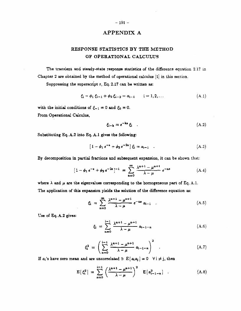
- 191 -
APPENDIX A
RESPONSE STATISTICS BY THE l\1ETHOD
OF OPERATIONAL CALCULUS
The transient and steady-state response statistics of the difference equation 2.17 in
Chapter 2 are obtained by the method of operational calculus [1] in this section.
Suppressing the superscript r, Eq. 2.17 can be written as:
with the initial conditions of e-l =0 and eo =o.From Operational Calculus,
Substituting Eq. A.2 into Eq. A.l gives the following:
i = 1,2, ... (A.I)
(A.2)
(A.3)
By decomposition in partial fractions and subsequent expansion, it can be shown that:
(AA)
where A and p. are the eigenvalues corresponding to the homogeneous part of Eq. A.!.
The application of this expansion yields the solution of the difference equation as:
(A.S)
Use of Eq. A.2 gives:
2
(~ Ao+1 _ p.o+l )
e? = L- A ai-l-o0=0 - p.
If ai's have zero mean and are uncorrelated:;, E [aiaj] = 0 'V i :1= j, then
E [e,?] = ~ (AO+: __ p.0+l)2L- A E(a~_l_O] .
0=0 p.
(A.6)
(A.7)
(A.B)

- 192 -
In addition, the ei'S have zero mean (taking expectation of Eq. A.6) . .If the input process
ai has a constant standard deviation U a Vi I then
where
(A.9)
From Eq.2.17:
(A.IO)
Therefore,
(A.ll)
if'1i and Ii have zero mean and are uncorrelated.
Furthermore, if '71 and Ii have constant standard deviations u" and (7/, respectively, Vi,
then
(A.12)
In fact, the assumptions of zero mean and constant standard deviation for the input process
ai are implied by similar assumptions on '1i and Ii and Eq. A.lO.
From Eqs. A.9 and A.12:
(A.13)
Back-substituting for Ai, a and (3:
(A.14)
Equation A.14 defines the variance for the transient response corresponding to the difference
equation A.1.
Steady state response statistics are obtained by letting i -+ 00 in Eq. A.l3:
(A.IS)

- 193 -
in which
Aoo
= 00 (>.n+l _ ~n+l) 2
2:= >._~n=O
00
= 1 2: [>.2(n+l) + ~2(n+l) _ 2(>.~)n+ll(>' - ~)2 n=O
If the system is stable, then 1>'1 < 1 and I~I < 1, and so:
1 [>'2 ~2Aco = (>' _ ~)2 1 _ >.2 + 1 _ ~2
which simplifies to:
2>'~ ]1 - >.~
(1 + >.~)Aco = -:---~~--.;~--~(1 - >.2) (1 - ~2) (1 - >.~)
Therefore, the steady state response variance is given by:
2 (1 + >.~)tT(_ = (1 _ >.2) (1 _ ~2) (1 _ >.~)
[(Atwr)<40 2 (At)<40 2]* Q' + tTl(1 + At frwr)2 " (1 + Atfrwr)2
provided that 1>'1 < 1 and I~l < 1.
The eigenvalues of the difference equation A.l are calculated as follows:
and the eigenvalues are:
>., ~ =i [tPl ± VtP~ - 4tIJz ]
where tPl and t/J'J are given by Eq.2.17.
Case (i) tP~ - 4tP2 < 0 ( Wr < l* VI - {; )i.e., the eigenvalues are complex conjugates.
1>'1 = I~I =i [tPi + (4t/J'J - tPi) ]1/2
= [t/J'J]1/2
= [1 -At fr Wr ] 1/2 < 11 + At fr Wr
(A.16)
(A.17)
(A.I8)
(A.I9)
(A.20)

- 194-
Case (ii) 4>1 - 44>2 = a ( Wr = it JI - s'"; )
Le., the eigenvalues are real and coincident.
IA= J.' = - 4>1
2
_ 1 - j (~twr)2
- 1 + ~ts'"rwr
so JAI, IJ.'I < 1 if ~twr < 2.
Case (iii) 4>1 - 44>2 > 0 ( Wr > lt J1 - s'"; )
Le., the eigenvalues are real and distinct.
A, J.' = ~ [4>1 ± V4>1 - 4</>2 ]
= (1+ A1tr,,,,,) [1- i (At",,? { 1 'f
so IAI, 1J.&1 < 1 if Atwr < J2.
• Example Problem
For Case (i) described previously,
(A.2I)
(A.22)
,\ = 4[4>1 +i V44>2 - 4>r ]
J.& = 4[4>1 - i V4</>2 - 4>r ]
Using Eqs. 2.17, A.23 and A.16:
A _ (1 + dts'"r wr)200 - (~twr)3)r [4 - (~twr)2]
Then from Eq. A.17:
Therefore,
(A.23)
(A.24)
(A.25)

- 195 -
REFERENCE
[1] Erdelyi, A., Operational Calculus and Generalized Functions, Holt, Rinehart and Winston, Inc., 1962.

CALIFORNIA INSTITUTE OF TECffiDLCGY
Reports Published
by
Earthquake Engineering Research Laboratory*Dynamic Laboratory
Disaster Research Center
Note: Numbers in parenthesis are Accession Numbers assigned by theNational Technical Information Service; these reports may be orderedfrom the National Technical Information Service, 5285 Port Royal Road,Springfield, Virginia, 22161. Accession Numbers should be quoted onorders for reports (PB --- ---). Reports without this informationeither have not been submitted to m'IS or the information was not available at the time of printing. An NVA in parenthesis indicates that thereport is no longer available at caltech.
1. Alford, J.L., G.W. Housner and R.R. Martel, "Spectrum Analysis ofStrong-~lotion Earthquake," 1951. (Revised August 1964). (N/A)
2. Housner, G.W., "Intensity of Ground Motion During Strong Earthquakes," 1952. (N/A)
3. Hudson, D.E., J.L. Alford and G.W. Housner, "Response of a Structure to an Explosive Generated Ground Shock," 1952. (N/A)
4. Housner, G.W., "Analysis of the Taft Accelerogram of the Earthquake of 21 July 1952." (N/A)
5. Housner, GoW., "A Dislocation Theory of Earthquakes," 1953. (~VA)
6• caughey, T.K., and D.E. Hudson, "An Electric Analog Type ResponseSpectrum," 1954. (NVA)
7. Hudson, D.E., and G.W. Housner, ''Vibration Tests of a Steel-FrameBuilding," 1954. (N/A)
8. Housner, GoW., "Earthquake Pressures on Fluid Containers," 1954.(N/A)
9. Hudson, D.E., "The Wilmot Survey Type Strong-r4otion EarthquakeRecorder," 1958. (N/A)
10. Hudson, D.E., and w.o. Iwan, "The Wilmot SUrvey Type Strong-r-lotionEarthquake Recorder, Part II," 1960. (NVA)
* To order directly by phone the number is 703-487-4650.

11. Caughey, T.K., D.E. Hudson, and ReV. Powell, "The CIT Mark IIElectric Analog Type Response Spectrum Analyzer for Eartll:1uakeExcitation Studies," 1960. (N/A)
12. Keightley, W.o., G.W. Housner and D.E. Hudson, "Vibration Tests ofthe Encino Dam Intake TOwer," 1961. (N/A)
13. Merchant, Howard carl, "Mode SUperposition Methods Applied toLinear Mechanical systems Under Earth:Iuake Type Excitation," 1961.(WA)
14. Iwan, Wilfred D., "The Dynamic Response of Bilinear Hystereticsystems," 1961. (N/A)
15. Hudson, D.E., "A New Vibration Exciter for Dynamic Test of Full-scale Strl.1ctures," 1961. (N/A) .
16. Hudson, D.E., "Synchronized Vibration Generators for Dynamic Testsof Full-scale Structures,n 1962. (N/A)
17. Jennings, Paul c., "Velocity Spectra of the Mexican Earth:Iuakes of11 May and 19 May 1962," 1962. (N/A)
18. Jennings, Paul c., "Response of Simple Yielding Structures toEartl'quake Excitation,n 1963. (N/A)
19. Keightley, Willard 0., "Vibration Tests of Structures," 1963.(N/A)
20. caughey, T.K., and M.E.J. O'Kelly, nGeneral Theory of Vibration ofDamped Linear Dynamic systems,n 1963. (N/A)
21. O'Kelly, M.E.J., "Vibration of Viscously Damped Linear Dynamicsystems," 1964. (N/A)
22. Nielsen, N. Norby, "Dynamic Response of Miltistory Buildings,"1964. (N/A)
23. '1'50, Wai Keung, "Dynamics of Thin-Walled Beams of Open Section,"1964. (N/A)
24. Keightley, Willard 0., "A Dynamic Investigation of BO\.XIuet canyonDam," 1964. (N/A)
25. Malhotra,~, "Free and Forced Oscillations of a Class of SelfExcited Oscillators," 1964.
26. Hanson, Robert D., "Post-Elastic Response of Mild Steel Structures," 1965.
27. Masri, sami F., nAnalytical and Experimental Studies of ImpactDampers, n 1965.
RERJRl'S-2

28. Hanson, Robert D., "Static and Dynamic Tests of a full-SCaleSteel-Frame Structures," 1965.
29. Cronin, Donald 1., "Response of Linear, Viscous Damped Systems toExcitations Having Time-Varying Fr6:!uecy," 1965.
30. Hu, Paul Yu-fei, "Analytical and Experimental Studies of RandomVibration," 1965.
31. Crede, Charles Ee, "Research on Failure of Equipment when Subjectto Vibration," 1965.
32. Lutes, Loren D., "Numerical Response Characteristics of a UniformBeam Carrying one Discrete Load," 1965. (N/A)
33. Rocke, Richard D., "Transmission Matrices and Lumped ParameterModels for Continuous Systems," 1966. (N/A)
34. Brady, Arthur Gerald, "Studies of Response to E'artlxIuake GroundMotion," 1966. (N/A)
35. Atkinson, John D., "Spectral Density of First Order PiecewiseLinear Systems Excited by White Noise," 1967. (N/A)
36. Dickerson, John Re, "Stability of Parametrically Excited Differential Equations, " 1967. (N/A)
37. Giberson, Melbourne F., "The Response of Nonlinear Multi-StoryStructures Subjected to Earth;{uake Excitation," 1967. (N/A)
38. Ha1langer, Lawrence w., "The Djnamic Stability of an UnbalancedMass Exciter," 1967.
39. Husid, Raul, "Gravity Effects on the E'arth;{uake Response of Yielding Structures," 1967. (N/A)
40. Kuroiwa, Julio fl., "Vibration Test of a Multistory Building,"1967. (N/A)
41. Lutes, Loren Daniel, "Stationary Random Response of Bilinear Hysteretic Systems," 1967.
42. Nigam, Navin c., "Inelastic Interactions in the Dynamic Responseof Structures," 1967.
43. Nigam, Navin C. and Paul C. Jennings, "Digital Calculation ofResponse Spectra from Strong-Motion Earth;{uake Records," 1968.
44. Spencer, Richard 'A., "The Nonlinear Response of SOme MultistoryReinforced and Prestressed Concrete Structures Subjected to Parthquake Excitation," 1968. (&lA)
REroRTS-3

45. Jennings, P.c., G.W. Housner and Nee. Tsai, "Simulated Earth:iuakeMotions," 1968.
46. "Strong-Motion Instrumental Data on the Borrego Mountain Earthquake of 9 April 1968," (USGS and EERL Joint Report), 1968.
47. Peters, Rex 13., "Strong Motion Accelerograph Evaluation, II 1969.
48. Heitner, Kenneth Le, "A Mathematical Model for callculation of theRun-Up of Tsunamis," 1969.
49. Trifunac, Mihailo D., "Investigation of Strong Earthquake GroundMotion," 1969. (N!A)
50. Tsai, Nien Clien, "Influence of Local Geology on Earthquake GroundMotion," 1969. (N!A)
51. Trifunac, Mihailo D., "Wind and Microtremor Induced Vibrations ofa Twenty-Two Steel Frame Building," EERL 70-01, 1970.
52. Yang, I-Min, "Stationary Random Response of Multidegre~of-FreedomSystems," DYNrr-100, June 1970. (N/A)
53. Patula, Edwatd John, "Equivalent Differential Equations for Nonlinear Dynamic Systems," DYNL-10l, June 1970.
54. Prelewicz, Daniel h3am, "Range of Validity of the r-lethod of Averaging," DYNL-102, 1970.
55 Trifunac, M.D., "On the Statistics and Possible Triggering Mechanism of Earthquakes in Southern California," EERL 70-03, July 1970.
56. Heitner, Kenneth Leon, "Additional Investigations on a Mathematical Model for calculation of Run-Up of Tsunamis," July 1970.
57. Trifunac, Mihailo D., "Ambient Vibration Tests of a Thirty-NineStory Steel Frame Building," EERL 70-02, July 1970.
58. Trifunac, Mihailo D. and D.E. HUdson, "Laboratory Evaluations andInstrument Corrections of Strong-Motion Accelerographs," EERL 7004, August 1970. (N!A)
,59. Triftmac, Mihailo D., "Response Envelope Spectrum and Interpreta
tion of Strong Earthquake Groun Motion," EERL 70-06, August 1970.
60. Keightley, w.o., "A Strong-Motion Acce1erograph Array with Telephone Line Interconnections," EERL 70-05, september 1970.
61. Triftmac, Mihailo D., "Low Frequency Digitization Errors and a NewMethod for Zero Baseline Correction of Strong-Motion Accelerograms, It EEm. 70-07, september 1970.
REroRTS-4

62. Vijayaraghavan, A., "Free and Forced Oscillations in a Class ofPiecewise-Linear Dynamic Systems," DYNL-103, January 1971.
63. Jennings, Paul c., ReB. Mathiesen and J. Brent Hoerner, "ForcedVibrations of a 22-Story Steel Frame Building," EERt 71-01, February 1971. (N/A) (PB 205 161)
64. Jennings, Paul c., "Engineering Features of the san FernandoEarth:juake of February 9, 1971," EERL 71-02, June 1971. (PB 202550)
65. Bielak, Jacobo, "Eartb:;ruake Response of Building-Foundation Systerns," EERL 71-04, June 1971. (N/A) (PB 205 305)
66. Adu, Fando1ph lIdemo1a, "Response and Failure of Structures UnderStationary Random Excitation," EERL 71-03, June 1971. (N/A) (PB205 304)
67. Skattum, Knut Sverre, "Dynamic Analysis of Coupled Shear Walls andsandwich Beams," EERL 71-06, June 1971. (N/A) (PB 205 267)
68. Hoerner, John Brent, "Model Coupling and Eartb:;ruake Response ofTall Buildings," EERL 71-07, June 1971. (N/A) (PB 207 635)
69. Stahl, Karl John, "Dynamic Response of Circular Plates Subjectedto Moving Massive Loads," DYNl:t-104, June 1971. (N/A)
70. Trifunac, M.D., F.E. Udwadia and A.G. Brady, "High FrequencyErrors and Instrument Corrections of Strong-Motion Accelerograms,"EERL 71-05, 1971. (PB 205 369)
71. Furuike, D.Me, "Dynamic Response of Hysteretic Systems With Applicatioo to a System Containing Limited Slip," DYNL-105, September1971. (N/A)
72. Hudson, D.E. (Editor), "Strong-Motion Instrumental Data on the SanFernando Farth:juake of February 9, 1971," (Seismological FieldSurvey, roM, c.I.'r. Joint Report), September 1971. (PB 204 198)
73. Jennings, Paul C. and Jacobo Bielak, "Dynamics of Building-SoilInteraction," EERL 72-01, April 1972. (m 209 666)
74. Kim, Byung-Koo, "Piesewise Linear Dynamic Systems with Time Delays," DYNL-106, April 1972. .
75. Viano, David Charles, "Wave Propagation in a Symmetrically LayeredElastic Plate," DYNl:t-107, May 1972.
76. Whitney, Albert W., "On Insurance Settlements Incident to the 1906san Francisco Fire, It DRe 72-01, August 1972. (PB 213 256)

77. Udwadia, F.E., "Investigation of Ear~uake and Microtremor GroundMotions," EERL 72-02, September 1972. (PB 212 853)
78. Wood, John H., "Analysis of the Ear~uake ResFOnse of a NineStory Steel Frame Building During the san Fernando Eart!l:luake,"EERL 72-04, OCtober 1972. (PB 215 823)
79. Jennings, Paul e., "Rapid Calculation of Selected Fourier SpectrumOrdinates," EERL 72-05, November 1972.
80. "Research Papers Submitted to Fifth World Conference on Eartix;IuakeEngineering, Rome, Italy, 25-29 June 1973," EERL 73-02, March1973. (PB 220 431) .
8~. Udwadia, F.E., and M.D. Trifunac, '-rhe Fourier Transform, ReSFCnseSpectra and '!heir Relationship Through the Statistics of Oscillator Response," EERL 73-01, April 1973. (FE 220 458)
82. Housner, George W., "Earth;Iuake-Resistant Design of High-RiseBuildings," DRC 73-01, July 1973. (WA)
83. "Earth;Iuake and Insurance," Farth;Iuake Research Affiliates Conference, 2-3 April, 1973, DRC 73-02, July 1973. (PB 223 033)
84. Wood, John H., "Earth;Iuake-Induced SOil Pressures on Structures,"EERL 73-05, August 1973. (tVA)
85. Crouse, Charles 8., "Engineering Studies of the san FernandoEarth;Iuake," EERL 73-04, March 1973. (N/A)
86. Irvine, H.Max, "'!he Veracruz Earth;Iuake of 28 August 1973," Em.73-06, OCtober 1973.
87. Iemura, H. and P.e. Jennings, "Hysteretic Resp:lnse of a Nine-StoryReinforced Concrete Building During the san Fernando Earth:luake,"EERL 73-07, OCtober 1973.
88. Trifunac, M.D. and V. Lee, "Routine Complter Processing of StrongMotion Accelerograms," EERL 73-03, OCtober 1973. (N/A) (PB 226o47/AS)
89. Moeller, 'Ihomas Lee, "The Dynamics of a Spinning Elastic Disk withMassive Load," DYNL 73-01, OCtober 1973.
90. Blevins, Rebert D., "Flow Iriduced Vibration of Bluff Structures,"DYNL 74-01, February 1974.
91. Irvine, H. Max, "Studies in the Statics and Dynamics of Simplecable Systems," DYNL-108, January 1974.

92. Jephcott, D.l<. and D.E. Hudson, "'!he Performance of Public SchoolPlants During the san Fernando Eart.h:Iuake," EERL 74-01, September1974. (PB 240 aaa/AS)
93. Wong, Hung Leung, "Dynamic Soil-Structure Interaction," EERL 7501, May 1975. (N/A) (PB 247 233/AS)
94. Foutch, D.A., G.W. Housner, and P.e. Jennings, "Dynamic Responsesof Six Multistory BUildings During the san Fernando Earti'quake,"EERL 75-02, OCtober 1975. (PS 248 144/AS)
95. Miller, Richard Keith, "'!he Steady-State Response of Multidegreeof-Freedom Systems with a Spatially Localized Nonlinearity," EERL75-03, OCtober 1975. (PB 252 459/AS)
96. Abdel-Ghaffar, Ahmed Mansour, "Dynamic Analyses of SuspensionBridge Structures," EERL 76-01, May 1976. (PB 258 744/AS)
97. Foutch, Douglas A., "A Study of the Vibrational Characteristics ofTwo Multistory Buildings," EERL 76-03, september 1976. (PB 260874/AS)
98. "Strong Motion Eart.h:Iuake Accelerograms Index Volume," EarthquakeEngineering Research Laboratory, EERL 76-02, August 1976. (PB 260929/AS)
99. Spanos, P-T.D., "Linearization Techniques for Non-Linear DjnamicalSystems," EERL 76-04, september 1976. (PB 266 083/AS)
100. Edwards, Dean Barton, "Time Domain Analysis of SWitching Regulators," DYNL 77-01, March 1977.
101. Abdel-Ghaffar, Ahmed Mansour, "Studies of the Effect of Differential Motions of Two Foundations upon the Response of the Superstructure of a Bridge," EERL 77-02, January 1977. (PS 271 095/AS)
102. Gates, Nathan c., "'!he Earth::Iuake Response of Deteriorating Systems," EERL 77-03, March 1977. (l:B 271 090/AS)
103. Daly, w., W. Judd and R. Meade, "Evaluation of Seismicity at u.S.Reservoirs," USOJLt), Committee on EartixIuakes, May 1977. (PB 270036/AS)
104. Abdel-Ghaffer, A.M. and G.W. Housner, "An Analysis of the DjnamicCharacteristics of a SUspension Bridge by Ambient Vibration Measurements," EERL 77-01, January 1977. (l:B 275 063/AS)
105. Housner, G.W. and P.e. Jennings, "EartixIuake Design Criteria forstructures," EERL 77-06, November 1977. (PB 276 502/AS)
REroRTS-7

106. Morrison, P., R. Maley, G. Brady, R. Porcella, "Earth:juake Recordings on or Near Darns, II UsroLD, Committee on Eartiquakes, November1977. (PB 285 867/AS)
107. Abdel-Ghaffar, A.M., ''Engineering Data and Analyses of the Whittier, california Earth:juake of January 1, 1976," EERL 77-05,November 1977. (PB 283 750/~)
108. Beck, James Le, "Determining Models of Structures from Earth:IuakeRecords," EERL 78-01, June 1978. (PB 288 806/AS)
109. Psycharis, Ioannis, "'!he 5alonica(ThessaloniJd) Earth:juake of June20, 1978," EERL 78-03, OCtober 1978. (PB 290 120/AS)
110. Abdel-Ghaffar, A.M. and R.F. SCott, "An Investigation of theDynamic Characteristics of an Earth Darn," EERL 78-02, August 1978.(PB 288 878/AS
Ill. Mason, Alfred Be, Jr., "Some Cbservations on the Random Responseof Linear and Nonlinear DynamIcal Systems," EERL 79-01, January1979. (PB 290 808/~)
ll2. Helmberger, D.V. am P.e. Jennings (Organizers), "Strong GroundMotion: N.5.F. Seminar-Workshop," SL-EERL 79-02, February 1978.
113. Lee, David Me, Paul e. Jermings and George W. Hausner, rcA Selection of Important Strong Motion Earth:Iuake Records," EERL 80-01,January 1980. (PB 80 169196)
114. McVerry, Graeme IL, ""Frequency Domain Identification of StructuralModels from Earth::J:uake Records," EERL 79-02, OCtober 1979. (PB80-194301)
115. Abdel-Ghaffar A.M., ReF.Scott and M.J.Craig, "Full-SCalI Experimental Investigation of a Modern Earth Dam," EERL SO-02, February1980 • (PB-81-123788)
ll6. Rutenberg, Avigdor, Paul e. Jermings and George W. Housner, ''TheResponse of Veterans Hospital Building 41 in the San FernandoEartb::Juake," EERL 80-03, May 1980. (PB-82-201377)
117. Haroun, Medhat Ahmed, "Dynamic Analyses of Liquid Storage 'lanks,"EERL 80-04, February 1980. (PB-81-123275)
118. Liu, Wing Karo, "Development of Finite Element Procedures forFluid-Structure Interaction, If EERL 80-06, August 19S0. em184078)
119. Yoder, Paul Jerome, itA Strain-Space Plasticity Theory and Numerical Implementation," EERL 80-07, August 1980. (PB-82-201682)
120. Krousgrill, Charles Morton, Jr., "A Linearization Technique forthe Dynamic Response of Nonlinear Continua," Em.. 80-0S, September1980. (PB-82-20l823)
'~:ORTS-8

121. Cohen, Martin, "Silent Boundary Methods for Transient Wave Analysis," EERL 80-09, September 1980. (PB-82-201831)
122. Hall, Shawn A., ''Vortex-Induced Vibrations of Structures," EERL81-01, January 1981. Cffio-82-201849)
123. Psycharis, Ioannis No., "Dynamic Behavior of Rocking StructuresAllowed to Uplift," EERL 81-02, August 1981. (PB-82-212945)
124. Shih, Choon-Foo, "Failure of Liquid Storage 'lanks Due to Earthquake Excitation," EERL 81-04, May 1981. (PB-82-215013)
125. Lin, Albert Niu, "Experimental c:l:>servations of the Effect ofFOlmdation Embedment on Structural Response," EERL 82-01, May1982. (PB-84-163252)
126. Botelho, Dirceau 1.R., "An Empirical Model for Vortex-InducedVibrations," EERL 82-02, August 1982. (PB-84-161157)
127. Ortiz, 1. Alexander, "Dynamic Centrifuge Testing of cantileverRetaining Walls," SML 82-02, August 1982. (PB-84-162312)
128. Iwan, W.o., Editor, "Proceedings of the u.s. National Workshop onStrong-Motion Farth::luake Instrumentation, April 12-14, 1981, santaBarbara, california," california Institute of Technology,Pasadena, California, 1981.
129. Rashed, Ahmed, "Dynamic Analysis of Fluid-Structure Systems, II EERL82-03, July 1982. (PB-84-162916)
130. National Academy Press, "Ear~uake Engineering Research-1982."
131. National Academy Press, "Earth::Juake Engineering Research-1982,Overview and Recommendations."
132. Jain, SUdhir Kumar, "Analytical Models for the Dynamics of Buildings," EERL 83-02, May 1983. (PB-84-161009)
133. Huang, Moh-Jiann, "Investigation of Local Geology Effects onStrong Earthquake Ground Motions," EERL 83-03, July 1983. (PB-84161488)
134. Mcverry, G.H. and J.L. Beck, "Structural Identification of JPLBuilding 180 Using Optimally Synchronized Earth::luake ~ords."
EERL 83-01, Au9USt 1983. (PB-84-162833)
135. Bardet, J.P., "Application of Plasticity 'lheory to SOil Behavior:A New sand Model," SML 83-01, september 1983. (H3-84-1623 04)

136.
137.
138.
139.
140.
141.
Wilson, John c., "Analysis of the Cbserved Earthquake Resp:mse ofa Multiple Span Bridge,1I EERL 84-01, ~1ay 1984. (PB-85-240505/AS)
Hushmand, Behnam, IIExperimental Studies of Dynamic Response ofFoundations," SML 83-02, November 1983. (PB-86-115383/N
Cifuentes, Arturo 0., "System Identification of Hysteretic Structures," EERL 84-04, 1984. (PB-240489/AS14)
Smith, Kenneth SCott, "Stochastic Analysis of the Seismic Responseof Secondary Systems," EERL 85-01, November 1984. (PB-85240497/AS)
~1aragakis, Emmanuel, "A Model for the Rigid Body Hotions of Ske~'J
Bridges,1I EERL 85-02, December 1984. (PB-85-248433/AS)
Jeong, Garrett Duane, "cumulative Damage of Structures Subjectedto Response Spectrum Consistent Random Process, II EERL 85-03,January 1985. (PB-86-100809)
142.
143.
Chelvakumar, Kasivisvanathan, "A Simple Strain-Space PlasticityModel for Clays, It EERL 85-05, 1985. PB-
Pak, Ronald Y.s., "Dynamic Response of a Patially Embedded BarUnder Transverse Excitations," EERL 85-04, May 1985. PB-
144. Tan, Thiam-Soon, "Two Phase Soil Study: A. Finite Strain Consolidation, B. Centrifuge scaling Considerations," SML 85-01, August1985. PB-
145. Iwan, Wilfred D., Michael A. Moser and Chia-Yen Peng, IIStrongMotion Ear~uake Measurement Using a Digital Accelerograph, II EERL84-02, April 1984.
146. Beck, ReT. and J.L. Beck, "Comparison Between Transfer Functionand Modal Minimization Methods for System Identification," EERL85-06, April 1984.
147. Jones, Nicholas Patrick, "Flow-Induced Vibration of LongStructures," DYNL 86-01, May 1986. PB-
148. Peek, Ralf, "Analysis of Unanchored Liquid Storage Tanks UnderSeismic Loads," EERL 86-01, April 1986. PB-
149. Paparizos, Leonidas G., "Some O:>servations on the Random Responseof Hysteretic Systems, II EERL 86-02. PB-
REK>RrS-10

Strong-Motion Earthquake AccelerogramsDigitized and Plotted Data
Uncorrected Accelerograms
Volume I
ABCDEFGHIJKLMNopQRSTUVWXY
Report. No.
EERL 70-20EERL 70-21EERL 71-20EERL 71-21EERL 71-22EERL 71-23EERL 72-20EERL 72-21EERL 72-22EERL 72-23EERL 72-24EERL 72-25EERL 72-26EERL 72-27EERL 73-20EERL 73-21EERL 73-22EERL 73-23EERL 73-24EERL 73-25EERL 73-26EERL 73-27EERL 73-28EERL 73-29EERL 73-30
REroRl'S-11
Nl'ISAccession. No.
PB 287 847PB 196 823PB 204 364PB 208 529PB 209 749PB 210 619PB 211 357PB 211 781PB 213 422PB 213 423PB 213 424PB 215 639PB 220 554PB 223 023PB 222 417PB 227 481/ASPB 232 315/ASPB 239 585/ASPB 241 551/ASPB 241 943/ASPB 242 262/ASPB 243 483/ASPB 243 497/ASPB 243 594/ASPB 242 947/AS

Strong-Motion Ear~uake Acce1erogramsDigitized and Plotted Data
Corrected l\ccelerograms and IntegratedGround Velocity and Displacement Clrves
VOlume· II
ABCDEFGHI
J,KL,MN
O,PQ,R
STUV
W,Y
Report ~.
EERL 71-50EERL 72-50EERL 72-51EERL 72-52EERL 73-50EERL 73-51EERL 73-52EERL 74-50EERL 74-51EERL 74-52EERL 74-53EERL 74-54EERL 74-55EERL 74-56EERL 74-57EERL 75-50EERL 75-51EERL 75-52EERL 75-53
REroRTS-12
NI'ISAccession ~.
m 208 283PB 220 161m 220 162PB 220 836PB 223 024PB 224 977/9ASPB 229 239/ASPB 231 225/ASPB 232 316/ASPB 233 257/ASm 237 174/ASPB 236 399/ASm 239 586/ASPB 239 587/ASm 241 552/ASPB 242 433/ASPB 242 949/ASFa 242 948/ASPB 243 719

Analyses of Strong-Motion Earttquake kcelerogramsResponse Spectra
VOlume III
ABCDEFGHI
J,K,LM,NO,PQ,R
STUV
W,Y
Report. No.
BERt 72-80EERL 73-80BERt 73-81EERL 73-82BERt 73-83EERL 73-84EERL 73-85EERL 74-80EERL 74-81EERL 74-82EERL 74-83EmL 74-84Em. 74-85EERL 74-86Em. 75-80EmL 75-81EERL 75-B2BERt 75-83
I ~: .•
Nl'ISkcession No.
m 212 602I?B 221 256m 223 025PB 227 469/ASm 227 470/ASPB 227 471/ASm 231 223/ASPB 231 319/ASm 232 326/ASPB 236 110/ASPB 236 400/115PB 238 102/ASm 240 68B/ASPB 241 553/ASm 243 69B/ASPB 242 950/ASfB 242 951/ASPB 243 492/AS

Analyses of Strong-Motion E'arth::Iuake AccelerogramsFourier ~itude Spectra
VQ1yme.IY
NrIS~ Report No. Accession No.
A EERL 72-100 m 212 603B EERL 73-100 PB 220 837C EERL 73-101 m 222 514D EERL 73-102 PB 222 969/ASE EERL 73-103 PB 229 240/ASF EERL 73-104 PB 229 241/ASG EERL 73-105 m 231 224/~
H EERL 74-100 PB 232 327/ASI EERL 74-101 PB 232 328/AS
J,K,L,M EERL 74-102 PB .236 Ill/ASN,O,P EERL 74-103 m 238 447/~Q,R,S EERL 74-104 PB 241 554/AS
T,U EEm, 75-100 PB 243 493/ASV,W,Y EERL 75-101 PB 243 494/AS
Index Volume EERL 76-02
REEORTS-14
PB 260 929/~


![Pseudo Limits, Biadjoints, and Pseudo Algebras: Categorical ...arXiv:math/0408298v4 [math.CT] 18 Oct 2006 Pseudo Limits, Biadjoints, and Pseudo Algebras: Categorical Foundations of](https://img.dokumen.tips/doc/110x75/60a7a6d20b1ec1029337c248/pseudo-limits-biadjoints-and-pseudo-algebras-categorical-arxivmath0408298v4.jpg)