Embed Size (px)
Citation preview

April 2006
Research Report: UCPRC-RR-2005-06
Calibration of Incremental-Recursive Flexible Damage Models in CalME
Using HVS Experiments
Authors:Per Ullidtz, Dynatest Consulting Inc
John Harvey, UC DavisBor-Wen Tsai, UC Berkeley
Carl Monismith, UC Berkeley
This work was completed as part of Partnered Pavement Research Program Strategic Plan Element 4.1:
“Development of the First Version of a Mechanistic-Empirical Pavement Rehabilitation, Reconstruction and New Pavement Design Procedure for Rigid and Flexible Pavements
(pre-Calibration of AASHTO 2002)”
PREPARED FOR:
California Department of Transportation Division of Research and Innovation Office of Roadway Research
PREPARED BY:
University of California Pavement Research Center
Berkeley and Davis

Stage 5 Distribution
UCPRC-RR-2005-06 ii
DOCUMENT RETRIEVAL PAGE Report No: UCPRC-RR-2005-06
Title: Calibration of Incremental-Recursive Flexible Damage Models in CalME Using HVS Experiments
Authors: Per Ullidtz, Dynatest Consulting Inc.; John Harvey, UC Davis; Bor-Wen Tsai, UC Berkeley; and Carl Monismith, UC Berkeley Prepared for: California Department of Transportation Division of Research and Innovation Office of Roadway Research
FHWA No.: F/CA/RR/2006/49
Date:Stage 5, May 2007
Contract number: UCPRC-RR-2005-06
Client Reference No: UCPRC-RR-2005-06
Status:Final, Caltrans approved
Abstract: Caltrans is in the process of implementing Mechanistic-Empirical design procedures. All mechanistic-empirical methods must be validated/calibrated against the behavior of real pavements. This should be done before implementing models in design methods to ensure that designs will be reasonable. The Heavy Vehicle Simulator (HVS) provides a first step in this validation/calibration process. The short test section can be carefully constructed with well characterized materials and instrumented to measure the pavement response. The climatic conditions may be controlled or monitored closely and all load applications are known exactly. The pavement may also be tested until it fails. The HVS may be seen as “large scale” laboratory equipment, between the “small scale” laboratory equipment (triaxial tests, bending tests etc.) and the reality of real pavements, which have uncertainties regarding materials, loads and climatic conditions. The two HVSs owned by Caltrans have been used on 27 flexible pavement test sections, with varying combinations of asphalt and granular layers. Temperature control was used during the tests. Most sections have been instrumented with Multi-depth Deflectometers (MDDs) to compare the measured pavement deflections (at several depths) to the deflections predicted by mechanistic methods, during the full duration of tests carried to “failure” (in terms of rutting or cracking). Results from mechanistic models have been compared with the deflection measurements and performance as a first step prior to empirical calibrations with field results. The complete time history of each test has been compared rather than just the beginning and end measurements. This report presents the validation of the mechanistic models for asphalt fatigue and for permanent deformation with the HVS test results.
Keywords: Mechanistic-empirical, full-scale-testing, calibration, response, performance, flexible pavement .
Proposals for implementation: None
Related documents: Kannekanti, V., and Harvey, J. June 2005. Sensitivity Analysis of 2002 Design Guide Rigid Pavement Distress Prediction Models. Draft report prepared for the California Department of Transportation. Pavement Research Center, Institute of Transportation Studies, University of California Berkeley, University of California Davis. UCPRC-RR-2005-01
Signatures: P. Ullidtz Principal Author
J. Harvey Co-principal Investigator
C. L. Monismith Co-principal Investigator
D. Spinner Editor
M. Samadian Caltrans Contract Mgr.

Stage 5 Distribution
UCPRC-RR-2005-06 iii
DISCLAIMER
The contents of this report reflect the views of the authors who are responsible for the facts and accuracy of the data presented herein. The contents do not necessarily reflect the official views or policies of the State of California or the Federal Highway Administration. This report does not constitute a standard, specification, or regulation.

Stage 5 Distribution
UCPRC-RR-2005-06 iv
EXECUTIVE SUMMARY
The first step in a mechanistic-empirical (ME) pavement design or evaluation is to calculate pavement response — in terms of stresses, strains, and/or displacements — using a mathematical (or mechanistic) model. In the second step, the calculated response is used as a variable in empirical relationships to predict structural damage (decrease in moduli or cracking) and functional damage (rutting and roughness) to the pavement.
Both of these steps must be reasonably correct. If the calculated response bears little resemblance to the pavement’s actual response, there is no point in trying to use the calculation to predict future damage to the pavement. In other words, only if the calculated response is reasonably correct does it make sense to try to relate the damage to the pavement response.
This study’s purpose was to evaluate the overall trends of the damage models in the draft software package called CalME against those of Heavy Vehicle Simulator (HVS) tests for which data was available.The report presents simulations of HVS tests using the set of distress models included in CalME. These models are for the typical flexible pavement distresses observed in California: asphalt fatigue, asphalt rutting, unbound layers rutting, and reflection cracking. An Incremental-Recursive approach (see item 4 below) was used for the simulations included in this report because this approach can accurately indicate pavement condition at different points during a pavement’s life.
Approaches Included in CalME
CalME software provides the user with four approaches to evaluating or designing a flexible pavement structure:
1. Caltrans’ current methods: the R-value method for new flexible structures and the deflection reduction method used by Caltrans for overlay thickness design for existing flexible pavements.
2. “Classical” Mechanistic-Empirical (ME) Design, which is based largely on the Asphalt Institute Method which uses very simple methods to characterize materials, climate, and traffic inputs.
3. An Incremental approach, which is a standard Miner’s Law approach that permits damage calculation for the axle load spectrum and expected temperature regimes, but without updating of the material’s properties through the life of the project. This is an approach similar to the one for cracking of asphalt included in the NCHRP 1-37A Pavement Design Guide, also referred to as the Mechanistic-Empirical Design Guide (MEPDG). This type of approach is calibrated against an end failure state (such as, 25 percent cracking of the wheelpath) and it assumes a linear accumulation of damage to get to that state.
4. An Incremental-Recursive approach in which the materials properties of the pavement — in terms of damage and aging — are updated as the pavement life simulation progresses.
The current Caltrans methods and the Classical method are very fast in terms of computational time, and user input is highly simplified. In CalME both of these options perform a “design” function, calculating and presenting pavement structures that meet the design requirements for the design traffic, materials, and climate.
For design practice the Classical and Caltrans methods should be used to produce a set of potential pavement sections. The Incremental-Recursive method should then be run to check the lowest-cost alternative designs in the set to be certain that they meet design requirements. Once the final design has been selected, its Incremental-Recursive output provides a prediction of the pavement condition across its entire life. The prediction of the pavement’s condition through its life from the Incremental-Recursive output can be used as the first prediction for use in a pavement management system.

Stage 5 Distribution
UCPRC-RR-2005-06 v
Use of Heavy Vehicle Simulator Data to Evaluate Models
The Incremental-Recursive models included in CalME were used to predict performance for all twenty-seven of the flexible pavement HVS tests performed so far as part of the Accelerated Pavement Testing (APT) program operated for the California Department of Transportation (Caltrans) by the University of California Pavement Research Center (UCPRC). The HVS test data in this report come from tests performed between the years 1995 and 2004. The HVS response data and corresponding laboratory test data were extracted from the UCPRC HVS database.
During HVS testing, pavement response - in terms of deflections at the surface and/or at multiple depths - may be measured. A Road Surface Deflectometer (RSD) measures deflections at the surface and is similar to the Benkelman Beam used to develop the current Caltrans overlay design method in the 1950s. A Multi-depth Deflectometer (MDD) measures deflections at multiple depths.
In order to accurately predict the gradual degradation of a pavement, the response model must predict measured deflections with reasonable accuracy. Although a model might predict deflections correctly, this ability does not guarantee that the model can also accurately predict the stresses and strains in all the pavement layers. However, the opposite is true: if a model predicts deflections incorrectly it will also produce incorrect stress and strain predictions. Therefore when attempting to calibrate ME models from HVS tests, the research team’s first concern was to make sure that resilient deflections were predicted reasonably well for the duration of the test and for all load levels. This prediction depended on the moduli of all the pavement layers and on the changes to the moduli caused by fatigue damage, slip between asphalt layers, non-linear elastic characteristics of unbound layers, and the effect of confinement on granular layers. Once reasonably good agreement was achieved between the measured and the calculated deflections then the permanent deformation models could be calibrated with confidence.
Differences in boundary conditions, strain levels, and loading times, all of which can produce varied effects in materials, result in differing moduli values. In this study, methods used for determining moduli (also referred to as “stiffness”) values included backcalculation from Falling Weight Deflectometer (FWD) and MDD data, and direct measurement — employing laboratory triaxial testing for unbound materials and flexural frequency sweep testing for asphaltic materials. Stiffnesses for the study’s asphalt materials were taken primarily from flexural frequency sweep data. Stiffnesses for the unbound layers came primarily from MDD data backcalculation.
In practice the FWD is seen by the research team as the primary tool for stiffness measurement of all layers already constructed because it is used in the field on the full pavement system; this is thought to be appropriate because the boundary conditions are those of real pavement, and most Caltrans’ work will be rehabilitation and reconstruction with at least some layers already in place. The research team saw the flexural beam test as the primary means for measuring the stiffness and fatigue characteristics of asphalt overlay materials for new layers. For new pavement construction, a combination of FWD testing on existing pavements and triaxial testing can be used to develop a database of stiffnesses of unbound granular layers and subgrades based on different characteristics, such as Unified Soil Classification System (USCS) classification.
The purpose of this study was to evaluate the overall trends of the CalME damage models against those of the HVS test results. This was accomplished by comparing deflections calculated using moduli determined from initial measurements and CalME damage calculations with measured deflections under HVS loading. The results presented in this report verify that, overall, the CalME damage trends for deflection and permanent deformation under loading are correct.
During HVS testing, deflections often increase markedly, sometimes becoming more than twice as high at the end of the test as they were at the beginning because of damage to the asphalt concrete caused by the repeated wheel loads. However, the flexible pavement design model of the NCHRP 1-37A Design Guide does not consider any decrease in the asphalt modulus as a result of fatigue damage (except for rehabilitation designs). In fact, the NCHRP 1-37A Design Guide includes a model for aging that predicts a continuous increase in the stiffness of the asphalt concrete layers across the life of the pavement, which results in increased stiffness and smaller predicted deflections as the pavement is subjected to trafficking. While the
Stage 5 Distribution
UCPRC-RR-2005-06 vi
aging is potentially important, the effect of updating stiffness for aging and not updating it for fatigue damage results in calculation of very unrealistic elastic responses in the pavement during its life. This makes it impossible to use the model to simulate an HVS test and, inversely, to use HVS tests to calibrate the model, except for pavements with extremely thick asphalt concrete layers where little fatigue should develop.
Results of HVS Test Simulation Using CalME
The series of HVS tests in this report are grouped here by goals, which are defined as follows:
• Goal 1, a comparison of new pavement structures with and without asphalt-treated permeable base (ATPB) layer under dry conditions, moderate temperatures, 20°C (HVS Sections 500RF, 501RF, 502CT, 503RF)
• Goal 3 Cracking, a comparison of reflection cracking performance of ARHM-GG (the acronym ARHM, asphalt rubber hot-mix gap-graded, refers to the material specification at the time of construction in April 1997.) and dense-graded asphalt concrete (DGAC) overlays placed on the cracked Goal 1 sections, dry conditions, 20°C (HVS Sections 514RF, 515RF, 517RF, 518RF)
• Goal 3 Rutting, a comparison of rutting performance of ARHM-GG and DGAC overlays of previously untrafficked areas of Goal 1 pavements, dry conditions, 40°C or 50°C at 50-mm depth, four different tire/wheel types (HVS Sections 504RF, 505RF, 506RF, 507RF, 508RF, 509RF, 510RF, 511RF, 512RF, 513RF)
• Goal 5, a comparison of new pavement structures with and without ATPB layer under wet conditions (water introduced into base layers), moderate temperatures, 20°C (HVS Sections 543RF, 544RF, 545RF)
• Goal 9, initial cracking of asphalt pavement with six replicate sections in preparation for later overlay, new pavement, ambient rainfall, 20°C (HVS Sections 567RF, 568RF, 569RF, 571RF, 572RF, 573RF)
CalME models that the simulations evaluated included:
• A stiffness model for asphalt concrete modulus as a function of reduced time based on the model used in NCHRP 1-37A Design Guide, with some adjustments based on field observations;
• An asphalt concrete fatigue model that predicts damage, in terms of decrease in modulus, as a function of load repetitions, tensile strain, and stiffness, using parameters from flexural beam testing;
• An ability to model partial bonding between asphalt concrete layers;
• A model that adjusts the stiffness of unbound layers as a function of the combined bending resistance (a function of their stiffness and thickness) of the layers above them;
• A model that adjusts the stiffness of unbound layers as a function of load level, with an increased load level increasing the moduli for the granular layers and decreasing modulus for the subgrade (clay);
• A permanent deformation model for asphalt concrete as a function of permanent shear strain near the pavement surface beneath the edge of a tire, with permanent shear strain predicted by the calculated elastic shear strain and elastic shear stress;
• A permanent deformation model for unbound layers as a function of the vertical strain at the top of each layer; and
• A reflection cracking model based on tensile strain calculated using a regression equation developed from a large number of Finite Element analyses and the same damage parameters developed for asphalt concrete fatigue.

Stage 5 Distribution
UCPRC-RR-2005-06 vii
Response Models
During most of the HVS tests, resilient deflections were measured using the RSD and the MDD. The following figure summarizes the measured deflections with those calculated using CalME damage models for all of the sections in terms of the ratio of the initial deflections before HVS loading to the final deflections at the end of the loading.
Assumptions made regarding differences between moduli from different measurement methods, shift factors, slip between layers, and non-linear elasticity of unbound layers to obtain reasonably good agreement between measured resilient deflections and those calculated with CalME are discussed in the report.
The observed behavior of the aggregate base (AB) and subbase layers under HVS loading contradicts the commonly accepted wisdom for granular materials, which is based primarily on triaxial testing. The observed behavior is discussed in the report and is modeled in CalME.
Using these assumptions, it was possible to model resilient deflections reasonably well for the full history of all of HVS test sections using the layered elastic analysis program (LEAP) response model.
Final/initial deflection
0.00
1.00
2.00
3.00
4.00
5.00
0.00 1.00 2.00 3.00 4.00 5.00
Measured
Cal
cula
ted
RSDMDDEquality
Figure ES-1. Ratio of initial to final deflection.
Damage of Asphalt Materials
Controlled strain fatigue tests conducted on beams were used to derive model parameters for the decrease in modulus for all the asphalt materials — except for the ATPB, where laboratory tests were not available. Working under the assumptions used in the modeling and using a shift factor with these damage models produced the correct changes in resilient deflections during all the HVS tests.

Stage 5 Distribution
UCPRC-RR-2005-06 viii
For reflection cracking, a simple model was used to calculate the strains in an overlay caused by existing cracking in the original top layer. Using this model and the laboratory fatigue model, reasonably correct resilient deflections were also predicted.
Relating visual cracking to the calculated asphalt damage proved to be difficult, and no single relationship could be derived. Goal 1 and Goal 5 showed differences between the drained and the undrained sections; for Goal 3 Cracking, the increase in visual cracking was quicker than for Goal 1 and Goal 5; and for Goal 9, visual cracking occurred at much less calculated damage than for the other experiments.
It is possible that the relationship between visual cracking and calculated damage depends on the thickness of the asphalt layers, and that reflection cracks and cracks in new pavements develop differently. It is also possible that the development of visual cracking depends on factors that the simulations did not consider.
No single relationship could be established between the relative increase in deflection and the amount of surface cracking (shown in the following figure), but it may be noted that visible cracking was not observed until deflection had increased by 50 percent or more.
Cracking versus relative deflection
0
2
4
6
8
10
12
1 1.5 2 2.5 3 3.5 4 4.5
Deflection/initial deflection
Cra
ckin
g m
/m2
500RF501RF502CT503RF514RF515RF517RF518RF543RF544RF545RF567RF568RF569RF571RF572RF573RF
Figure ES-2. Cracking versus increase in deflection.
Permanent Deformation of Asphalt
The following figure shows the measured and predicted final permanent deformation of the asphalt layers from Goal 1, Goal 3, and Goal 5, where data were available. Permanent deformation was calculated for the upper 100 mm of the asphalt layer(s).

Stage 5 Distribution
UCPRC-RR-2005-06 ix
Permanent deformation in AC (pro rated)
0
2
4
6
8
10
12
14
16
18
20
0 2 4 6 8 10 12 14 16 18 20
Measured, mm
Cal
cula
ted,
mm
Equality20 ºC at surface45 or 50 ºC at surface
Figure ES-3. Measured and predicted final permanent deformation of asphalt.
In Figure ES-3, the 20°C outlier point with a measured deformation greater than the calculated one is Section 543RF, which was a wet, drained test where the ATPB stripped and collapsed. The two relatively low values at high temperatures are from the test with a bias-ply dual tire and from the test with an aircraft tire. The correlation coefficient between measured and calculated values is 0.82 and the standard error of estimate is 2.2 mm.
The parameters for predicting permanent shear strain were based on Repeated Simple Shear Tests at Constant Height (RSST-CH).
Permanent Deformation of Granular Layers The permanent deformation of the granular layers for Goal 1, Goal 3, and Goal 5 are shown with
average measured values in Figure ES-4. It should be noted that the permanent deformations are rather small except for Section 543RF, the wet drained section, where the permanent deformation includes part of the ATPB.

Stage 5 Distribution
UCPRC-RR-2005-06 x
Permanent deformation of granular layers
0
2
4
6
8
10
12
14
0 2 4 6 8 10 12 14
Measured, mm
Cal
cula
ted,
mm
Goal 1Goal 3Goal 5Equality
Figure ES-4. Final permanent deformation of granular layers.
Permanent deformation was calculated both at the top of the AB and at the top of the aggregate subbase (ASB). The two materials are rather similar and might have been treated as a single layer.
Permanent Deformation of Subgrade
The final permanent deformation of the subgrade is even smaller than that of the granular layers, with a maximum measured value of less than 2 mm. In addition, the data scatter is as large as that of the granular layers, with an average coefficient of variation of 70 percent. This is far from ideal for the calibration of a subgrade permanent deformation model. The mean measured and predicted final deformations are shown in Figure ES-5. The subgrade and granular results indicate that rutting of the unbound layers is probably not a major concern for existing Caltrans pavements that need rehabilitation unless there is poor drainage or significant amounts of water are entering cracks in the asphalt layers.

Stage 5 Distribution
UCPRC-RR-2005-06 xi
Permanent deformation of subgrade
0.0
0.5
1.0
1.5
2.0
2.5
3.0
0.0 0.5 1.0 1.5 2.0 2.5 3.0
Measured, mm
Cal
cula
ted,
mm
Figure ES-5. Final permanent deformation of the subgrade.
Total Permanent Deformation at Pavement Surface
Figure ES-6 shows the final calculated permanent deformation at the pavement surface versus the measured final deformation averaged from profilometer measurements along the HVS test area.
Calculated final permanent deformations that underestimated the measured final permanent deformations were worst for the Goal 5 sections in which water was dripped into the base layers, especially for the drained section, 543RF in which the ATPB stripped.
The correlation coefficient between measured and calculated deformations is 0.61 and the standard error of estimate is 2.6 mm.
Conclusions and Recommendations
The overall results from this study indicate that Incremental-Recursive models provide reasonable results when predicting the response and performance of pavement under HVS loading. However, now that the models have been shown to match the mechanics of the flexible pavements under HVS loading, additional work remains to be done before these models can be used for pavement design and performance prediction.
There are significant differences between HVS testing and field results, and the approach used in this study has limitations because of those differences. These include the effects of age and of seasonal variation that have not been quantified in the simulations because HVS tests are of relatively short duration and are performed, to varying degrees, in controlled environments. Field calibration is required to evaluate the response difference between the field pavement and the Incremental-Recursive simulation that should be attributed to aging and seasonal effects. It is likely that the effects of aging can be dealt with using shift factors.

Stage 5 Distribution
UCPRC-RR-2005-06 xii
Permanent deformation at pavement surface
0.0
5.0
10.0
15.0
20.0
0.0 5.0 10.0 15.0 20.0
Measured, mm
Cal
cula
ted,
mm
Goal 1 Goal 3 45/55°CGoal 3 20°C Goal 5Goal 9 Equality
Figure ES-6. Final permanent deformation at the pavement surface.
The effects of rest periods between loadings and of faster traffic have also not been included in the calibration. It is expected that different shift factors will result because of rest periods and different trafficking patterns.
Lastly, moduli from frequency sweep data, triaxial tests, FWD tests, and MDD deflections used in this study are similar but they are not identical. The NCHRP 1-37A Design Guide study proposes relying primarily on triaxial testing to characterize the stiffness of flexible pavement layers and the permanent deformation parameters of asphaltic materials.
Recommendations are made in this report for the most practical and economical methods for characterizing materials based on the understanding that the majority of Caltrans’ work over the next several decades will be rehabilitation and reconstruction, with some addition of lane capacity.
Recommendations are also made regarding the next steps to develop the CalME models. These include:
1. Perform a sensitivity analysis using “typical” values for properties and climate in the database established to date, and compare the results from the Classical, Incremental, and Incremental-Recursive methods included in CalME to evaluate reasonableness of sensitivity across the three methods.
2. Simulate mainline highway case studies and test track data (such as WesTrack and NCAT track) using the recommended methods for characterizing flexible pavement materials in conjunction with the Incremental-Recursive models in CalME, and compare the simulated and measured results, as was done for the HVS results presented in this report. This step will provide validation for the models

Stage 5 Distribution
UCPRC-RR-2005-06 xiii
3. Address the variability of the input parameters (moduli, thicknesses, traffic loading, etc.) and uncertainty on the damage models. Several approaches should be considered, including the approach used in the NCHRP 1-37A method.
4. Make final decisions regarding use of cemented layers in the flexible pavement structure, then calibrate. It is generally recommended that “semi-rigid” pavements, in which asphalt concrete is placed directly on cement-treated base (CTB) or lean concrete base (LCB), not be used because of the relatively quick reflection of shrinkage cracks. However, because Caltrans has used semi-rigid pavements in the past and they remain in the current design method, it is therefore important to have models for the response and performance of these layers. The models in the NCHRP 1-37A Report should be the starting point for such a validation-and-calibration exercise.

Stage 5 Distribution
UCPRC-RR-2005-06 xiv
TABLE OF CONTENTS
Executive Summary............................................................................................................................................. iv Approaches Included in CalME ...................................................................................................................... iv Use of Heavy Vehicle Simulator Data to Evaluate Models ............................................................................. v Results of HVS Test Simulation Using CalME ..............................................................................................vi
Response Models........................................................................................................................................vii Damage of Asphalt Materials .....................................................................................................................vii Permanent Deformation of Asphalt ...........................................................................................................viii Permanent Deformation of Granular Layers................................................................................................ ix Permanent Deformation of Subgrade ........................................................................................................... x Total Permanent Deformation at Pavement Surface....................................................................................xi
Conclusions and Recommendations................................................................................................................xi List of Figures...................................................................................................................................................xvii List of Tables .................................................................................................................................................... xxv 1.0 Introduction............................................................................................................................................. 1
1.1 Models and Approaches Included in CalME .......................................................................................... 1 1.1.1 Validation Using Heavy Vehicle Simulator Data .......................................................................... 2
1.2 HVS tests................................................................................................................................................. 4 1.2.1 Goal 1 and Goal 3 Tests ................................................................................................................. 4 1.2.2 Goal 5 Tests ................................................................................................................................... 6 1.2.3 Goal 9 Tests ................................................................................................................................... 7
1.3 Response and Damage Models ............................................................................................................... 8 1.3.1 Asphalt Modulus ............................................................................................................................ 8 1.3.2 Fatigue.......................................................................................................................................... 21
1.4 Weak Bonding....................................................................................................................................... 24 1.5 Unbound Layers .................................................................................................................................... 25
1.5.1 Triaxial Tests................................................................................................................................ 25 1.5.2 Influence of Stiffness of Layers above an Unbound Layer.......................................................... 26 1.5.3 Influence of Load Level ............................................................................................................... 39
1.6 Permanent Deformation ........................................................................................................................ 40 1.6.1 Asphalt ......................................................................................................................................... 40 1.6.2 Unbound Materials....................................................................................................................... 47
1.7 Reflection Cracking .............................................................................................................................. 48 2.0 Goal 1 Cracking Test Simulations ........................................................................................................ 50
2.1 Goal 1 Resilient Deformations.............................................................................................................. 50

Stage 5 Distribution
UCPRC-RR-2005-06 xv
2.1.1 Section 501RF Resilient Deflections (Undrained)....................................................................... 50 2.1.2 Section 503RF Resilient Deflections (Undrained)....................................................................... 56 2.1.3 Section 500RF Resilient Deflections (Drained)........................................................................... 60 2.1.4 Section 502CT Resilient Deflections (Drained)........................................................................... 65
2.2 Visual Cracking Versus Damage of the Top Asphalt Layer, Goal 1 .................................................... 69 2.3 Goal 1 Permanent Deformation............................................................................................................. 72
2.3.1 Section 501RF Permanent Deformations..................................................................................... 73 2.3.2 Section 503RF Permanent Deformations..................................................................................... 75 2.3.3 Section 500RF Permanent Deformations..................................................................................... 77 2.3.4 Section 502CT Permanent Deformations..................................................................................... 79
3.0 Goal 3 Reflection cracking tests............................................................................................................ 81 3.1 Resilient Deflections ............................................................................................................................. 81
3.1.1 Section 517RF DGAC on Section 501RF Resilient Deflections ................................................. 81 3.1.2 Section 518RF ARHM on Section 503RF Resilient Deflections................................................. 86 3.1.3 Section 514RF DGAC on Section 500RF Resilient Deflections ................................................. 91 3.1.4 Section 515RF ARHM on Section 502CT Resilient Deflections ................................................ 96
3.2 Visual Cracking Versus Damage of the Overlay, Goal 3, 20ºC.......................................................... 101 3.3 Permanent Deformation Goal 3, 20ºC................................................................................................. 104
3.3.1 Section 517RF 75-mm DGAC Permanent Deformations .......................................................... 105 3.3.2 Section 518RF 38-mm ARHM Permanent Deformation ........................................................... 107 3.3.3 Section 514RF 75-mm DGAC Permanent Deformations .......................................................... 109 3.3.4 Section 515RF 38-mm ARHM Permanent Deformations ......................................................... 112
4.0 Goal 3 Rutting experiments................................................................................................................. 114 4.1 Section 504RF No Overlay, Wide-Base Single Tire........................................................................... 115 4.2 Section 505RF DAGC Overlay, Bias-Ply Dual Tire........................................................................... 117 4.3 Section 506RF DGAC Overlay, Radial Dual Tire .............................................................................. 119 4.4 Section 507RF DGAC Overlay, Wide-Base Single Tire .................................................................... 121 4.5 Section 508RF ARHM Overlay, Wide-Base Single Tire.................................................................... 123 4.6 Section 509RF ARHM Overlay, Radial Dual Tire ............................................................................. 125 4.7 Section 510RF ARHM Overlay, Radial Dual Tire ............................................................................. 127 4.8 Section 511RF ARHM Overlay, Wide-Base Single Tire.................................................................... 129 4.9 Section 512RF DGAC Overlay, Wide-Base Single Tire .................................................................... 131 4.10 Section 513RF DGAC Overlay, Aircraft Tire..................................................................................... 133
5.0 Goal 5 Wet conditions......................................................................................................................... 135 5.1 Section 543RF ARHM Overlay, Drained ........................................................................................... 136 5.2 Section 544RF ARHM Overlay, Undrained ....................................................................................... 145

Stage 5 Distribution
UCPRC-RR-2005-06 xvi
5.3 Section 545RF DGAC Overlay, Undrained ........................................................................................ 153 5.4 Visual Cracking versus Damage of the Top Asphalt Layer, Goal 5 ................................................... 160
6.0 Goal 9 Modified Binder (MB) road, initial tests ................................................................................. 162 6.1 Materials Characterization .................................................................................................................. 162 6.2 Section 567RF MB Road .................................................................................................................... 169 6.3 Section 568RF MB Road .................................................................................................................... 173 6.4 Section 573RF MB Road .................................................................................................................... 176 6.5 Section 571RF MB Road .................................................................................................................... 179 6.6 Section 572RF MB Road .................................................................................................................... 183 6.7 Section 569RF MB Road .................................................................................................................... 186 6.8 Visual Cracking Versus Damage of the Top Asphalt Layer, Goal 9 .................................................. 190
7.0 Summary and recommendations ......................................................................................................... 191 7.1 Shift Factors and Damage Equations Used in Simulations ................................................................. 191 7.2 Response Model .................................................................................................................................. 192 7.3 Damage of Asphalt Materials.............................................................................................................. 197 7.4 Permanent Deformation of Asphalt..................................................................................................... 199 7.5 Permanent Deformation of Granular Layers ....................................................................................... 201 7.6 Permanent Deformation of Subgrade.................................................................................................. 203 7.7 Total Permanent Deformation at Pavement Surface ........................................................................... 205 7.8 Recommendations ............................................................................................................................... 207
8.0 References ........................................................................................................................................... 209 9.0 Appendix............................................................................................................................................. 212
9.1 Glossary .............................................................................................................................................. 212 9.2 List of Units ........................................................................................................................................ 214 9.3 List of Parameters in Equations .......................................................................................................... 214 9.4 Parameter Values Used in Simulations ............................................................................................... 216 9.5 Section 569RF Simulated with a CTB Model from an HVS Nordic Experiment............................... 217

Stage 5 Distribution
UCPRC-RR-2005-06 xvii
LIST OF FIGURES
Figure ES-1. Ration of final to initial deflection ......................... ……………………………………………...vii
Figure ES-2. Cracking versus increase in deflection ......................... .……………………………………...…viii
Figure ES-3. Measured and predicted final permanent deflection of asphalt ........................... .....…………......ix
Figure ES-4. Final permanent deformation of granular layers ............................. ………………………………x
Figure ES-5. Final permanent deformation of the subgrade ............................. ……………………………...…xi
Figure ES-6. Final permanent deformation at the pavement surface............................ ……………………..…xii
Figure 1. Layout of 20°C test sections. Goal 3 rutting sections are distributed in the area between the 20°C test
sections. .......................................................................................................................................................4 Figure 2. Drip watering system for Goal 5 tests. .................................................................................................7 Figure 3. Layout of Goal 9 test sections. .............................................................................................................9 Figure 4. Example of modulus versus reduced time relationship. .....................................................................10 Figure 5. Modulus versus temperature for different viscosity versus temperature relationships.......................12 Figure 6. Frequency sweep data for Goal 1 and Goal 3 materials compared to models. ...................................13 Figure 7. Example of input parameters for the modulus-versus-reduced time relationship for the AC bottom
layer. 21 Figure 8. Example of damage versus number of load applications. ..................................................................23 Figure 9. Example of Equation 6 damage parameters of AC bottom layer (Goal 1). ........................................24 Figure 10. Simple Drucker-Prager failure condition..........................................................................................28 Figure 11. EAC 10,000 MPa, no slip, 40 kN load. ..............................................................................................29 Figure 12. EAC 10,000 MPa, slip, 40 kN............................................................................................................30 Figure 13. EAC 2,000 MPa, slip, 40 kN..............................................................................................................31 Figure 14. EAC 2,000 MPa, slip, 100 kN load. ...................................................................................................33 Figure 15. Displacement field in particulate sample...........................................................................................34 Figure 16. Displacement field in elastic solid (FEM). ........................................................................................35 Figure 17. Modulus of Layer 2 as a function of the stiffness of the asphalt layers, for the undrained sections.36 Figure 18. Modulus of Layer 2 as a function of the stiffness of the asphalt layers, for the drained sections. ...37 Figure 19. Modulus of subgrade as a function of the stiffness of the pavement layers. ....................................37 Figure 20. Results of RSST-CH tests. [Note: FMFC indicates field-mixed field compacted specimen taken by
coring the pavement. AV5.5 indicates cores with approximately 5.5 percent air-voids. Each title in the
legend indicates the RSST-CH test temperature (40, 50, or 60 °C) and average shear stress (MPa).] ......42 Figure 21. Normalized plastic strain versus number of load repetitions. (Note: legend is the same as in Figure
20). 44 Figure 22. Average values for Figure 21 curves. ...............................................................................................45 Figure 23. Best fitting Gamma function. (Note: legend is the same as in Figure 20 and Figure 21. .................46

Stage 5 Distribution
UCPRC-RR-2005-06 xviii
Figure 24. Input parameters for permanent deformation (rutting) of subgrade in second column. ...................48 Figure 25. Comparison of fitted vs. calculated strain for AC-on-AC overlay, 2D. ...........................................49 Figure 26. Section 501RF pavement structure...................................................................................................51 Figure 27. Section 501RF temperatures during testing......................................................................................52 Figure 28. Section 501RF 40 kN top modules deflection. .................................................................................52 Figure 29. Section 501 RF 40 kN resilient compression of pavement layers. ...................................................53 Figure 30. Section 501RF 40 kN deflection of subgrade...................................................................................53 Figure 31. Section 501RF 100 kN deflection of top modules............................................................................54 Figure 32. Section 501RF 100 kN resilient compression of pavement layers. ..................................................54 Figure 33. Section 501RF 100 kN deflection of subgrade.................................................................................55 Figure 34. Section 501RF calculated moduli at 40 kN and actual temperature. (Note: in this and all other
figures showing change in elastic moduli (E) under loading the lines are plotted for the modulus of each
layer, i.e., E1 is the modulus of the first layer, E2 is the modulus of the second layer, etc.).....................55 Figure 35. Section 503RF pavement structure...................................................................................................56 Figure 36. Section 503RF temperatures during testing......................................................................................56 Figure 37. Section 503RF 40 kN deflection of top modules..............................................................................57 Figure 38. Section 503RF 40 kN compression of pavement layers. ..................................................................57 Figure 39. Section 503RF 40 kN deflection of subgrade...................................................................................58 Figure 40. Section 503RF 100 kN deflection of top modules............................................................................58 Figure 41. Section 503RF 100 kN resilient compression of pavement layers. ..................................................59 Figure 42. Section 503RF 100 kN deflection of subgrade.................................................................................59 Figure 43. Section 503RF calculated layer moduli at 40 kN and actual temperature. .......................................60 Figure 44. Section 500RF pavement structure...................................................................................................60 Figure 45. Section 500RF temperatures during testing......................................................................................61 Figure 46. Section 500RF 40 kN deflection of top modules..............................................................................61 Figure 47. Section 500RF 40 kN resilient compression of pavement layers. ....................................................62 Figure 48. Section 500RF 40 kN deflection of subgrade...................................................................................62 Figure 49. Section 500RF 100 kN deflection of top modules............................................................................63 Figure 50. Section 500RF 100 kN compression of pavement layers. ................................................................63 Figure 51. Section 500RF 100 kN deflection of subgrade.................................................................................64 Figure 52. Section 500RF calculated moduli at 40 kN and actual temperature.................................................64 Figure 53. Section 502CT pavement structure...................................................................................................65 Figure 54. Section 502CT 40 kN deflection on top of AC. ...............................................................................65 Figure 55. Section 502CT 40 kN compression of pavement layers...................................................................66 Figure 56. Section 502CT 40 kN deflection of subgrade...................................................................................66 Figure 57. Section 502CT 100 kN deflection at top of AC. ..............................................................................67

Stage 5 Distribution
UCPRC-RR-2005-06 xix
Figure 58. Section 502CT 100 kN resilient compression of pavement layers. ..................................................67 Figure 59. Section 502CT 100 kN deflection of subgrade.................................................................................68 Figure 60. Section 502CT calculated moduli at 40 kN and 20ºC. .....................................................................68 Figure 61. Cracking versus relative decrease in modulus of top AC layer for Goal 1.......................................69 Figure 62. Goal 1, cracking versus increase in deflection. ................................................................................70 Figure 63. Permanent compression of AC layers. .............................................................................................73 Figure 64. Permanent compression of granular layers.......................................................................................73 Figure 65. Permanent deformation of subgrade.................................................................................................74 Figure 66. Permanent deformation at pavement surface....................................................................................74 Figure 67. Permanent compression of AC layers. .............................................................................................75 Figure 68. Permanent compression of granular layers.......................................................................................75 Figure 69. Permanent deformation of subgrade.................................................................................................76 Figure 70. Permanent deformation at pavement surface....................................................................................76 Figure 71. Permanent deformation of the AC layers. ........................................................................................77 Figure 72. Permanent compression of the granular layers. ................................................................................77 Figure 73. Permanent deformation of the subgrade. ..........................................................................................78 Figure 74. Permanent deformation at pavement surface....................................................................................78 Figure 75. Permanent compression of the AC layers.........................................................................................79 Figure 76. Permanent deformation of granular layers. ......................................................................................79 Figure 77. Permanent deformation of subgrade.................................................................................................80 Figure 78. Permanent deformation at surface of pavement. ..............................................................................80 Figure 79. Section 517RF pavement structure...................................................................................................82 Figure 80. Section 517RF AC temperature during testing.................................................................................82 Figure 81. Section 517RF 40 kN deflection of top modules..............................................................................83 Figure 82. Section 517RF 40 kN compression of pavement layers. ..................................................................83 Figure 83. Section 517RF deflection of subgrade..............................................................................................84 Figure 84. Section 517RF 100 kN top modules deflection. ...............................................................................84 Figure 85. Section 517RF 100 kN compression of pavement layers. ................................................................85 Figure 86. Section 517RF 100 kN deflection of subgrade.................................................................................85 Figure 87. Section 517RF calculated moduli at 40 kN and actual temperature.................................................86 Figure 88. Section 518RF pavement structure...................................................................................................86 Figure 89. Section 518RF AC temperature during testing.................................................................................87 Figure 90. Section 518RF 40 kN top modules deflection. .................................................................................87 Figure 91. Section 518RF 40 kN resilient compression of pavement layers. ....................................................88 Figure 92. Section 518RF 40 kN deflection of subgrade...................................................................................88 Figure 93. Section 518RF 100 kN top modules deflection. ...............................................................................89

Stage 5 Distribution
UCPRC-RR-2005-06 xx
Figure 94. Section 518RF 100 kN compression of pavement layers. ................................................................89 Figure 95. Section 518RF 100 kN deflection of subgrade.................................................................................90 Figure 96. Section 518RF calculated moduli at 40 kN and actual temperature.................................................90 Figure 97. Section 514RF pavement structure...................................................................................................91 Figure 98. Section 514RF AC temperature during testing.................................................................................91 Figure 99. Section 514RF 40 kN top modules deflection. .................................................................................92 Figure 100. Section 514RF 40 kN compression of pavement layers, MDD1 and MDD2.................................92 Figure 101. Section 514RF 40 kN compression of pavement layers, MDD3 and MDD4.................................93 Figure 102. Section 514RF 40 kN deflection of subgrade.................................................................................93 Figure 103. Section 514RF 100 kN top modules deflection. .............................................................................94 Figure 104. Section 514RF 100 kN compression of pavement layers, MDD1 and MDD2...............................94 Figure 105. Section 514RF 100 kN compression of pavement layers, MDD3 and MDD4...............................95 Figure 106. Section 514RF 100 kN deflection of subgrade...............................................................................95 Figure 107. Section 514RF calculated moduli at 40 kN and actual temperature...............................................96 Figure 108. Section 515RF pavement structure.................................................................................................96 Figure 109. Section 515RF AC temperature during testing...............................................................................97 Figure 110. Section 515RF 40 kN top modules deflection................................................................................97 Figure 111. Section 515RF 40 kN resilient compression of pavement layers. ..................................................98 Figure 112. Section 515RF 40 kN deflection of subgrade..................................................................................98 Figure 113. Section 515RF 100 kN top modules deflection. .............................................................................99 Figure 114. Section 515RF 100 kN compression of pavement layers. ..............................................................99 Figure 115. Section 515RF 100 kN deflection of subgrade.............................................................................100 Figure 116. Section 515RF calculated moduli at 40 kN and actual temperatures. ..........................................100 Figure 117. Cracking in overlay versus relative decrease in modulus of overlay, Goal 3. ..............................101 Figure 118. Goal 3, 20ºC, cracking versus increase in deflection....................................................................102 Figure 119. Section 517RF permanent deformation of AC layers...................................................................105 Figure 120. Section 517RF permanent deformation of granular layers. ..........................................................105 Figure 121. Section 517RF permanent deformation of subgrade. ...................................................................106 Figure 122. Section 517RF permanent deformation at pavement surface. ......................................................106 Figure 123. Section 518RF permanent deformation of AC layers...................................................................107 Figure 124. Section 518RF permanent deformation of granular layers. ..........................................................107 Figure 125. Section 518RF permanent deformation of subgrade. ...................................................................108 Figure 126. Section 518RF permanent deformation at pavement surface. ......................................................108 Figure 127. Section 514RF permanent deformation of AC layers...................................................................109 Figure 128. Section 514RF permanent deformation of granular layers, MDD1 and MDD2...........................109 Figure 129. Section 514RF permanent deformation of granular layers, MDD3 and MDD4...........................110

Stage 5 Distribution
UCPRC-RR-2005-06 xxi
Figure 130. Section 514RF permanent deformation of subgrade. ...................................................................110 Figure 131. Section 514RF permanent deformation at pavement surface. ......................................................111 Figure 132. Section 515RF permanent deformation of AC layers...................................................................112 Figure 133. Section 515RF permanent deformation of granular layers. ..........................................................112 Figure 134. Section 515RF permanent deformation of subgrade. ...................................................................113 Figure 135. Section 515RF permanent deformation of the pavement surface.................................................113 Figure 136. Section 504RF pavement structure...............................................................................................115 Figure 137. Section 504RF permanent deformation at pavement surface from profilometer..........................115 Figure 138. Section 504RF calculated permanent deformation of pavement layers........................................116 Figure 139. Section 505RF pavement structure...............................................................................................117 Figure 140. Section 505RF temperatures during testing..................................................................................117 Figure 141. Section 505RF permanent deformation at pavement surface from profilometer..........................118 Figure 142. Section 505RF calculated permanent deformation of pavement layers........................................118 Figure 143. Section 506RF pavement structure...............................................................................................119 Figure 144. Section 506RF temperatures during testing..................................................................................119 Figure 145. Section 506RF permanent deformation at pavement surface from profilometer..........................120 Figure 146. Section 506RF calculated permanent deformation of pavement layers........................................120 Figure 147. Section 507RF pavement structure...............................................................................................121 Figure 148. Section 507RF temperatures during testing..................................................................................121 Figure 149. Section 507RF permanent deformation at pavement surface from profilometer..........................122 Figure 150. Section 507RF calculated permanent deformation of pavement layers........................................122 Figure 151. Section 508RF pavement structure...............................................................................................123 Figure 152. Section 508RF temperatures during testing..................................................................................123 Figure 153. Section 508RF permanent deformation at pavement surface from profilometer..........................124 Figure 154. Section 508RF calculated permanent deformation of pavement layers........................................124 Figure 155. Section 509RF pavement structure...............................................................................................125 Figure 156. Section 509RF temperatures during testing..................................................................................125 Figure 157. Section 509RF permanent deformation at pavement surface from profilometer..........................126 Figure 158. Section 509RF calculated permanent deformation of pavement layers........................................126 Figure 159. Section 510RF pavement structure...............................................................................................127 Figure 160. Section 510RF temperatures during testing..................................................................................127 Figure 161. Section 510RF permanent deformation at pavement surface from profilometer..........................128 Figure 162. Section 510RF calculated permanent deformation of pavement layers........................................128 Figure 163. Section 511RF pavement structure...............................................................................................129 Figure 164. Section 511RF temperatures during testing..................................................................................129 Figure 165. Section 511RF permanent deformation at the pavement surface. ................................................130

Stage 5 Distribution
UCPRC-RR-2005-06 xxii
Figure 166. Section 511RF calculated permanent deformation of the pavement layers..................................130 Figure 167. Section 512RF pavement structure...............................................................................................131 Figure 168. Section 512RF temperatures during testing..................................................................................131 Figure 169. Section 512RF permanent deformation at pavement surface from profilometer..........................132 Figure 170. Section 512RF calculated permanent deformation of the pavement layers..................................132 Figure 171. Section 513RF pavement structure...............................................................................................133 Figure 172. Section 513RF permanent deformation at pavement surface from profilometer..........................134 Figure 173. Section 513RF calculated permanent deformation of pavement layers........................................134 Figure 174. Cores from trafficked area of Section 543RF after HVS loading show stripping and disintegration
of ATPB, as well as signs of moisture damage between the the three lifts of asphalt concrete (Bejarano et
al. 2003). ..................................................................................................................................................135 Figure 175. Section 543RF pavement structure...............................................................................................136 Figure 176. Section 543RF temperatures during testing..................................................................................137 Figure 177. Section 543RF Road Surface Deflectometer, at 40 kN. ...............................................................137 Figure 178. Section 543RF Road Surface Deflectometer, at 100 kN. .............................................................138 Figure 179. Section 543RF 40 kN top module. ...............................................................................................138 Figure 180. Section 543RF 40 kN top of aggregate base. ...............................................................................139 Figure 181. Section 543RF 40 kN top of aggregate subbase. ..........................................................................139 Figure 182. Section 543RF 40 kN deflection of subgrade (850 mm depth). ....................................................140 Figure 183. Section 543RF 100 kN top module. .............................................................................................140 Figure 184. Section 543RF 100 kN top of aggregate base. .............................................................................141 Figure 185. Section 543RF 100 kN top of aggregate subbase. ........................................................................141 Figure 186. Section 543RF 100 kN deflection of subgrade (850 mm depth). ..................................................142 Figure 187. Section 543RF Permanent deformation of asphalt layers.............................................................142 Figure 188. Section 543RF permanent deformation of granular layers plus top of subgrade..........................143 Figure 189. Section 543RF permanent deformation in subgrade (850 mm depth). ..........................................143 Figure 190. Section 543RF permanent deformation at pavement surface. ......................................................144 Figure 191. Section 543RF calculated layer moduli, at 40 kN and actual temperatures. ................................144 Figure 192. Section 544RF pavement structure...............................................................................................145 Figure 193. Section 544RF temperatures during testing..................................................................................145 Figure 194. Section 544RF Road Surface Deflectometer, at 40 kN. ...............................................................146 Figure 195. Section 544RF Road Surface Deflectometer, at 100 kN. .............................................................146 Figure 196. Section 544RF 40 kN top module. ...............................................................................................147 Figure 197. Section 544RF 40 kN top of aggregate base. ...............................................................................147 Figure 198. Section 544RF 40 kN top of aggregate subbase. ..........................................................................148 Figure 199. Section 544RF 100 kN top module. .............................................................................................148

Stage 5 Distribution
UCPRC-RR-2005-06 xxiii
Figure 200. Section 544RF 100 kN top of aggregate base. .............................................................................149 Figure 201. Section 544RF 100 kN top of aggregate subbase. ........................................................................149 Figure 202. Section 544RF Permanent deformation of asphalt layers.............................................................150 Figure 203. Section 544RF permanent deformation of aggregate base. ..........................................................150 Figure 204. Section 544RF permanent deformation on top of basecourse. ......................................................151 Figure 205. Section 544RF permanent deformation at pavement surface. ......................................................151 Figure 206. Section 544RF calculated moduli of pavement layers...................................................................152 Figure 207. Section 545RF pavement structure...............................................................................................153 Figure 208. Section 545RF temperatures during testing..................................................................................153 Figure 209. Section 545RF Road Surface Deflectometer, at 40 kN. ...............................................................154 Figure 210. Section 545RF Road Surface Deflectometer, 100 kN. .................................................................154 Figure 211. Section 545RF 40 kN top module. ...............................................................................................155 Figure 212. Section 545RF 40 kN top of aggregate base. ...............................................................................155 Figure 213. Section 545RF 40 kN top of aggregate subbase. ..........................................................................156 Figure 214. Section 545RF 100 kN top module. .............................................................................................156 Figure 215. Section 545RF 100 kN top of aggregate base. .............................................................................157 Figure 216. Section 545RF 100 kN top of aggregate subbase. ........................................................................157 Figure 217. Section 545RF permanent deformation of asphalt layers. ............................................................158 Figure 218. Section 545RF permanent deformation of aggregate base. ..........................................................158 Figure 219. Section 545RF permanent deformation at pavement surface. ......................................................159 Figure 220. Section 545RF calculated moduli of pavement layers..................................................................159 Figure 221. Visual cracking versus relative decrease in modulus of layer 1, Goal 5 Wet conditions. .............160 Figure 222. Goal 5, cracking versus increase in deflection. ............................................................................161 Figure 223. MB road, AC modulus-versus-reduced time parameters from frequency sweep. .........................162 Figure 224. Moduli from FWD compared to frequency sweep tests, Goal 9 (MB road). ................................163 Figure 225. MB road, damage parameters for AC in first column. ..................................................................165 Figure 226. MB road, backcalculated modulus of AB versus time. ................................................................166 Figure 227. MB road, modulus of AB versus stiffness of AC.........................................................................166 Figure 228. MB road, subgrade modulus versus stiffness of pavement layers. ................................................167 Figure 229. Section 567RF pavement structure................................................................................................169 Figure 230. Section 567RF load levels. ...........................................................................................................169 Figure 231. Section 567RF temperatures during testing...................................................................................170 Figure 232. Section 567RF Road Surface Deflectometer. ................................................................................170 Figure 233. Section 567RF MDDs at 90mm and 330 mm. .............................................................................171 Figure 234. Section 567RF permanent deformation of MDDs.........................................................................171 Figure 235. Section 567RF permanent deformation at pavement surface from profilometer...........................172
Stage 5 Distribution
UCPRC-RR-2005-06 xxiv
Figure 236. Section 567RF calculated moduli at 40 kN and actual temperature..............................................172 Figure 237. Section 568RF pavement structure................................................................................................173 Figure 238. Section 568RF temperatures during testing...................................................................................173 Figure 239. Section 568RF Road Surface Deflectometer. ................................................................................174 Figure 240. Section 568RF permanent deformation at pavement surface from profilometer...........................174 Figure 241. Section 568RF calculated layer moduli at 40 kN and actual temperature. ....................................175 Figure 242. Section 573RF pavement structure................................................................................................176 Figure 243. Section 573RF temperatures during testing...................................................................................176 Figure 244. Section 573RF Road Surface Deflectometer. ................................................................................177 Figure 245. Section 573RF permanent deformation at pavement surface from profilometer...........................177 Figure 246. Section 573RF calculated layer moduli at 40 kN and actual temperature. ....................................178 Figure 247. Section 571RF pavement structure................................................................................................179 Figure 248. Section 571RF temperatures during testing...................................................................................179 Figure 249. Section 571RF Road Surface Deflectometer. ................................................................................180 Figure 250. Section 571RF MDDs at 90 mm, 300 mm, and 525 mm. .............................................................180 Figure 251. Section 571RF permanent deformation of MDDs.........................................................................181 Figure 252. Section 571RF permanent deformation at the pavement surface. .................................................181 Figure 253. Section 571RF calculated layer moduli at 40 kN and actual temperature. ....................................182 Figure 254. Section 572RF pavement structure................................................................................................183 Figure 255. Section 572RF temperatures during testing...................................................................................183 Figure 256. Section 572RF Road Surface Deflectometer. ................................................................................184 Figure 257. Section 572RF permanent deformation at the pavement surface. .................................................184 Figure 258. Section 572RF calculated layer moduli at 40 kN and actual temperature. ....................................185 Figure 259. Section 569RF pavement structure................................................................................................186 Figure 260. Section 569RF temperatures during testing...................................................................................186 Figure 261. Section 569RF Road Surface Deflectometer. ................................................................................187 Figure 262. Section 569RF MDDs at 90 mm, 300 mm, and 525 mm ..............................................................187 Figure 263. Section 569RF permanent deformation of MDDs.........................................................................188 Figure 264. Section 569RF permanent deformation at pavement surface from profilometer...........................188 Figure 265. Section 569RF calculated layer moduli at 40 kN and actual temperature. ....................................189 Figure 266. Cracking versus relative decrease in modulus of AC layer for Goal 9 (MB road)........................190 Figure 267. Goal 9 (MB road), Cracking versus increase in deflection (RSD) ................................................190 Figure 268. Ratio of final over initial deflection. .............................................................................................195 Figure 269. Cracking versus calculated decrease in modulus of top layer. ......................................................197 Figure 270. Cracking versus increase in deflection. .........................................................................................198 Figure 271. Measured and predicted final permanent deformation of asphalt.................................................199

Stage 5 Distribution
UCPRC-RR-2005-06 xxv
Figure 272. Final permanent deformation of granular layers. .........................................................................201 Figure 273. Final permanent deformation of the subgrade. ..............................................................................203 Figure 274. Final permanent deformation at the pavement surface (profile data). ...........................................205 Figure 275. Modulus of AB layer backcalculated from FWD tests in center line. ...........................................217 Figure 276. Pavement structure for Section 569RF. .........................................................................................219 Figure 277. Damage parameters used for DGAC of Section 569RF. ...............................................................219 Figure 278. Damage parameters used for CTB of Section 569RF....................................................................220 Figure 279. Section 569RF Road Surface Deflectometer. ................................................................................220 Figure 280. Section 569RF MDD resilient deflections.....................................................................................221 Figure 281. Section 569RF permanent MDD deformations. ............................................................................221 Figure 282. Section 569RF average permanent deformation from pavement profile.......................................222 LIST OF TABLES
Table 1. Summary List of HVS Tests ...................................................................................................................3 Table 2. Design Thicknesses for Goal 1 Sections .................................................................................................5 Table 3. As-built Thicknesses for Goal 5 Sections ...............................................................................................6 Table 4. As-built Thicknesses of Goal 9 Sections ................................................................................................8 Table 5 Influence of Slip Value in LEAP on Calculated Vertical Deflections and Horizontal Strains .............25 Table 6. Triaxial Tests on Subgrade....................................................................................................................26 Table 7. Triaxial Tests on Aggregate Base (AB) ................................................................................................26 Table 8. Layer Thicknesses Used for FWD Backcalculation..............................................................................36 Table 9. Moduli Parameters from FWD .............................................................................................................38 Table 10. Moduli Parameters from Calibration to MDD Deflections.................................................................38 Table 11. Initial Moduli Used in HVS Simulations (MPa).................................................................................39 Table 12. Summary of Moduli (MPa).................................................................................................................39 Table 13. Parameters Used in Equation 20 .........................................................................................................41 Table 14. AC on AC, 2D Structural Parameter Combinations ...........................................................................49 Table 15. Initial Moduli MPa (1.8 km/h, 40 kN, Actual Temperature) for Each Section...................................71 Table 16. Final Moduli MPa (1.8 km/h, 40 kN, Actual Temperature) for Each Section....................................71 Table 17. Percentage Decrease in Layer Moduli for Each Section.....................................................................72 Table 18. Damage Parameter for Asphalt Layers at End of Test for Each Section ............................................72 Table 19. Initial Damage Parameters for “Old” Asphalt Overlay Sections ........................................................81 Table 20. Layered Moduli at Start of Test, MPa ..............................................................................................103 Table 21. Layer Moduli at End of Test, MPa ...................................................................................................103 Table 22. Percentage Decrease in Moduli ........................................................................................................104 Table 23. Initial Permanent Deformations, Goal 3, in mm...............................................................................104

Stage 5 Distribution
UCPRC-RR-2005-06 xxvi
Table 24. Tire Types and Pressure, MPa ..........................................................................................................114 Table 25. Estimated Temperatures for Section 513RF .....................................................................................133 Table 26. Parameters for FWD Moduli versus Reduced Time, Goal 9 ............................................................164 Table 27. MB Road, Stiffness Parameters for AB............................................................................................167 Table 28. Summary of Damage Equations and Shift Factors Used in All Simulations....................................192 Table 29. Measured and Calculated Road Surface Deflectometer Deflections (RSD), in mm.........................193 Table 30. Measured and Calculated Deflections of the Top Multi-depth Deflectometer (MDD), in mm........194 Table 31. Final Permanent Deformation of Asphalt, in mm.............................................................................200 Table 32. Final Permanent Deformation of Granular Layer, in mm.................................................................202 Table 33. Parameters used for Granular Materials in Equation (29) ................................................................202 Table 34. Final Permanent Deformation of Subgrade, in mm ..........................................................................204 Table 35. Parameters Used for Subgrade in Equation (29)...............................................................................204 Table 36. Final Permanent Deformation at the Pavement Surface, in mm.......................................................206

Stage 5 Distribution
UCPRC-RR-2005-06 1
1.0 INTRODUCTION
The first step in creating a Mechanistic-Empirical (ME) pavement design or evaluation is to calculate pavement response — in terms of stresses, strains, and/or displacements — using a mathematical (or mechanistic) model. In the second step, the calculated response is used as a variable in empirical relationships to predict structural damage (decrease in moduli or cracking) and functional damage (rutting and roughness) to the pavement.
Both of these steps must be reasonably correct. If the calculated response bears little resemblance to the pavement’s actual response, there is no point in trying to use the calculation to predict future damage to the pavement with the empirical relationship. In other words, only if the calculated response is reasonably correct does it make sense to try to relate the damage to the pavement response.
1.1 Models and Approaches Included in CalME
This report presents the modeling of several series of flexible pavement Heavy Vehicle Simulator (HVS) tests using the set of distress models included in the draft software package, CalME. These models are for the flexible pavement distresses typically observed in California: asphalt fatigue, asphalt rutting, unbound layers rutting and reflection cracking.
CalME software provides the user with four approaches for evaluating or designing a flexible pavement structure:
• Caltrans current methods, the R-value method for new flexible structures, and the deflection reduction method for overlay thickness design for existing flexible structures.
• “Classical” Mechanistic-Empirical (ME) design, largely based on the Asphalt Institute method. This method uses a standard Equivalent Single Axle Load (ESAL) for the traffic load, one temperature to characterize the entire range of temperatures the asphalt concrete (AC) layer will experience, and the Asphalt Institute fatigue and unbound layers rutting equations, with an adjustment for air-void content and binder content in the asphalt concrete.
• An Incremental method, using the typical Miner’s Law approach, permitting damage calculation for the axle-load spectrum and expected temperature regimes, but with no updating of materials properties through the life of the project. This is similar to the approach included in the NCHRP 1-37A Design Guide, also referred to as the Mechanistic-Empirical Pavement Design Guide (MEPDG). This type of approach is calibrated against an end failure state, such as 25 percent cracking of the wheelpath, and it assumes a linear accumulation of damage to get to that state.
• An Incremental-Recursive method in which the materials properties for the pavement are updated in terms of damage as the simulation of the pavement life progresses. The Incremental-Recursive approach was used for the simulations included in this report, and is the only approach that can provide an accurate indication of pavement condition at different points during the pavement’s life.
The research team proposes that pavement designers should begin their designs by applying either an existing Caltrans method or the Classical method. In CalME both of these options perform a “design” function, calculating and presenting pavement structures that meet design requirements for a predetermined number of traffic loads. Then, the lowest cost alternatives in the set of candidate pavement structures meeting the design requirements with either of these methods should be checked by the designer with the more comprehensive and precise Incremental-Recursive method to be certain that they meet the design requirements. Once a final design has been selected, its Incremental-Recursive output can be used to provide a prediction of the pavement’s condition across its entire life.
Some distresses and some materials are not considered in either the Caltrans or Classical methods, and can only be evaluated using the Incremental-Miner’s Law approach or the Incremental-Recursive approach.

Stage 5 Distribution
UCPRC-RR-2005-06 2
1.1.1 Validation Using Heavy Vehicle Simulator Data
The Incremental-Recursive models included in CalME were used to predict the performance of all the flexible pavement HVS tests performed to date as part of the Accelerated Pavement Testing (APT) program operated for the California Department of Transportation (Caltrans) by the University of California Pavement Research Center (UCPRC).
The HVS test data presented in this report come from tests performed between 1995 and 2004. The HVS response data and the corresponding laboratory test data were extracted from the UCPRC HVS database.
HVS tests measure pavement response in terms of deflections, either at the pavement surface, using a Road Surface Deflectometer (RSD), at multiple depths, using a Multi-depth Deflectometer (MDD), or both. The RSD is very similar to the Benkelman Beam used in the development of the Caltrans new flexible pavement and overlay design methods in the 1950s. In predicting the gradual degradation of the pavement it is important that the response model provides a reasonably accurate prediction of measured deflections. Although a correct prediction of deflections by the response model is no guarantee that it can also correctly predict the stresses and strains in all of the pavement layers, the opposite is true: if the model inaccurately predicts deflections, it will also provide inaccurate predictions of stresses and strains.
Therefore, in trying to calibrate the ME models from HVS testing, the research team’s first concern was to make sure that the model predicted resilient deflections reasonably well for the duration of the test and for all load levels. This prediction depended on the moduli (often referred to as “stiffnesses” in this report and in the literature) of all of the pavement layers and on the changes to these moduli caused by fatigue damage, slip between asphalt layers, non-linear elastic characteristics of the unbound layers, and the effect of confinement on granular layers. Once reasonable agreement was achieved between the measured resilient deflections and the calculated ones, then models of permanent deformation could be calibrated with some confidence.
There are different methods for determining moduli and there are often differences in the results from each method (which should be expected based on the literature.) The methods used in this study included backcalculation of moduli for all layers from Falling Weight Deflectometer (FWD) and MDD deflection data , and direct measurement of moduli in the laboratory using triaxial tests for unbound materials and flexural frequency sweep tests for asphaltic materials. Differences in measured moduli across the different methods are due to variations in boundary conditions, strain levels, and loading times between the different measurement methods, the effects of which vary among materials. The FWD does not fit under the HVS, so there is no FWD data during an HVS test, there is only FWD data from before the HVS was placed on the pavement and from after the HVS was taken off the trafficked section. The simulations in this report primarily relied on stiffnesses for the asphalt materials taken from flexural frequency sweep data, and stiffnesses for the unbound layers taken from backcalculation of MDD deflection data.
In practice, the research team views backcalculation using deflections from the FWD as the primary tool for obtaining the stiffnesses of layers in existing pavements, as opposed to laboratory testing of materials samples taken from the already constructed pavement. FWD deflections and backcalculation take into consideration the stiffness of the layers as they occur in the constructed pavement structure, including the effects of boundary conditions, water and temperature conditions, previous traffic and environmental conditioning, and interaction between layers acting as a system in the in-place pavement structure. This is important because most of Caltrans future work will be rehabilitating and reconstructing pavements already in service.
The research team sees the flexural beam test as the primary tool for measuring the stiffness and the fatigue characteristics of asphalt overlay materials for new layers. For new pavement construction, the team sees the use of databases of moduli for granular bases and subbases and for subgrades backcalculated from FWD tests on existing pavements, with the materials referenced by characteristics such as the Unified Soil Classification System (USCS) classification and relative density. The databases should also include some laboratory triaxial tests for these materials, for comparison with any new base, subbase, and subgrade materials

Stage 5 Distribution
UCPRC-RR-2005-06 3
for which there is no previous FWD testing, and for which laboratory triaxial testing must be used to measure stiffness.
The purpose of this study was to compare the overall trends shown by the damage models in simulations of the HVS tests against the actual trends measured in the same HVS tests. Asphalt concrete stiffnesses from flexural frequency sweep data were used in the simulations of the HVS tests, and the stiffnesses of the underlying moduli were adjusted from their initial values as the asphalt concrete stiffness changed with damage so they would match the measured and calculated deflections. The results presented herein show that, overall, the damage trends for deflection and permanent deformation under loading were verified.
During HVS testing, deflections often increase markedly, with deflection sometimes rising more than twice as high at the end of the test than they were at the beginning. The flexible pavement design model of the NCHRP 1-37A Design Guide (NCHRP 2004) does not consider any decrease in the asphalt concrete modulus as a result of fatigue damage (except for rehabilitation designs). In fact, the NCHRP 1-37A Design Guide includes a model for aging that predicts a continuous increase in the stiffness of asphalt concrete layers across the life of the pavement, resulting in smaller predicted deflections as the pavement is subjected to trafficking. While aging is potentially important, the effect of updating stiffness for aging and not updating it for fatigue damage results in the calculation of unrealistic elastic responses during the pavement life. This may be acceptable for pavements with extremely thick asphalt concrete layers where little fatigue should occur, but it is impossible to use the model to simulate an HVS test and, inversely, to use HVS tests to calibrate the model.
The HVS test series in this report were grouped by “goals,” which are defined as follows:
Table 1. Summary List of HVS Tests
Goal General Conditions HVS Test Numbers Original Report References
Goal 1: Comparison of structures with and without ATPB layer under dry conditions, moderate temperatures
New pavement, dry conditions, 20°C 500RF, 501RF, 502CT, 503RF
14, 15, 16, 17, 18
Goal 3 Cracking: Comparison of reflection cracking performance of ARHM-GG and DGAC overlays
Overlays of cracked Goal 1 sections, dry conditions, 20°C
514RF, 515RF 517RF, 518RF
8, 11, 13
Goal 3 Rutting: Comparison of rutting performance of ARHM-GG and DGAC overlays
Overlays of previously untrafficked areas of Goal 1 pavements, dry conditions, 40°C or 50°C at 50-mm depth, four different tire/wheel types
504RF, 505RF 506RF, 507RF 508RF, 509RF 510RF, 511RF 512RF, 513RF
7, 10
Goal 5: Comparison of structures with and without ATPB layer under wet conditions, moderate temperatures
New pavement, wet conditions, 20°C 543RF, 544RF, 545RF 2, 3, 4, 5, 13
Goal 9: Initial cracking of asphalt pavement in preparation for later overlay
New pavement, ambient rainfall, 20°C
567RF, 568RF, 569RF, 571RF, 572RF, 573RF
1
ATPB: Asphalt-treated permeable base. ARHM-GG: Asphalt-rubber hot-mix gap-graded. DGAC: Dense-graded asphalt concrete.

Stage 5 Distribution
UCPRC-RR-2005-06 4
The Goal 1, 3, and 5 tests were performed inside a metal shed built over native subgrade. The shed provided protection from sun, wind, and rain; however, changes in subgrade water content and the depth to the water table were recorded during HVS tests. Goal 9 tests were performed on a road with no cover other than what the HVS and its temperature cabinet provided.
The remainder of this chapter presents the general descriptions of the HVS tests and the models used to simulate them.
1.2 HVS tests
1.2.1 Goal 1 and Goal 3 Tests
Figure 1 shows the layout of the Goal 1 and Goal 3 cracking sections.
Figure 1. Layout of 20°C test sections. Goal 3 rutting sections are distributed in the area between the 20°C test sections.
All the sections in Goal 1 had two layers of asphalt concrete (AC), an aggregate base (AB), and an aggregate subbase (ASB). In the two drained sections, part of the AB layer thickness was replaced by an asphalt-treated permeable base (ATPB) at a ratio of 1.4:1.1. A constant temperature of about 20ºC was maintained during Goal 1. The design layer thicknesses are shown in Table 2.
518RF
517RF
515RF
514RF
503RF
501RF
502CT
500RF
Undrained Drained
ARHM-GG
DGAC
Goal1
Goal3

Stage 5 Distribution
UCPRC-RR-2005-06 5
Table 2. Design Thicknesses for Goal 1 Sections
Layer Undrained (mm) Drained (mm) AC top lift 61 61 AC bottom lift 76 76 ATPB None 76 AB 274 182 ASB 229 229
The subgrade was clay, with varying plasticity across the pavements.
Goal 3 was an overlay study with an aphalt rubber hot-mix gap-graded (ARHM-GG) (the acronym ARHM, asphalt rubber hot-mix gap-graded, refers to the material specification at the time of construction in April 1997.) concrete and a dense-graded asphalt concrete (DGAC). The four Goal 3 Cracking tests were performed at the same temperature as Goal 1 (20ºC), with similar wheel types and loads. For these tests the design thickness of the DGAC overlay (75 mm) was approximately twice as thick as that of the ARHM (40 mm), and the overlays were placed over the four previously cracked Goal 1 sections. The remainder of Goal 3 was done at higher temperatures, with the two overlays placed on previously untested areas of the Goal 1 pavement, and several overlay thicknesses, tire types, and wheel loads used in the testing. (Table 1 provides the reference numbers for the reports containing the details regarding thickness, tire types, and wheels loads.)
All the HVS tests at 20ºC started with a wheel load of 40 kN, which was increased stepwise to 100 kN. Most of the load applications were at 100 kN. Bias-ply tires on a dual wheel were used for the Goal 1 tests. The same radial tires on a dual wheel were used for the Goal 3 Cracking tests, and the Goal 5 and Goal 9 tests. Various tires and wheels were used for the Goal 3 Rutting tests, with the load for the entire duration of all but one test fixed at 40 kN. [De Beer and Fisher (1997) describe the details of the tire contact stresses measured.] For all the tests except the Goal 3 Rutting tests, the wheel load was a dual wheel with a centerline distance of 305 mm and an assumed tire pressure of 690 kPa for all load levels. It was assumed that the wheels distributed the load over two circular areas; this assumption was reasonably correct for the low load level (40 kN) but not for the high load level (100 kN, where the actual load distribution was closer to two rectangles with one side twice the length of the other).
All the 20°C sections were instrumented with MDDs. Each section in Goal 1 had two MDDs. Each section had two additional MDDs installed for Goal 3 testing. All MDD anchor depths were assumed to be 3,000 mm. Not all MDD modules functioned for the duration of the tests.
The as-constructed layer thicknesses given in Harvey et al. (1999) were used for the analyses of the Goal 1 and Goal 3 results presented in this report. As-built layer thicknesses given in Bejarano et al. (2003) and Bejarano et al. (2005) were used to analyze the Goal 5 and Goal 9 results respectively. The remaining data was imported from the UC Pavement Research Center database, taken from a subset database named PRC-HVS.mdb.
Although actual wheel speeds varied, they were assumed to be 7.6 km/h during HVS testing and 1.8 km/h during deflection measurement on the MDDs. All tests other than the Goal 3 Rutting tests were performed with bidirectional loading. The Goal 3 Rutting tests were performed with unidirectional loading.
The temperature of the test sections was controlled by a “temperature control box.” The actual temperatures of the asphalt layers were recorded and used in the simulations.
Poisson’s ratio was assumed to be 0.35 for all layers.

Stage 5 Distribution
UCPRC-RR-2005-06 6
1.2.2 Goal 5 Tests The Goal 5 tests were performed on the overlay structures of Goal 3 in locations where the overlay
had not been placed on previously trafficked and cracked Goal 1 pavement. The designed structures were:
• Section 543RF drained with ATPB and 40-mm ARHM-GG wearing surface,
• Section 544RF undrained (no ATPB) and 40-mm ARHM-GG wearing surface, and
• Section 545RF undrained (no ATPB) and 75-mm DGAC wearing surface.
The structures’ as-built thicknesses are shown in Table 3.
Table 3. As-built Thicknesses for Goal 5 Sections
Layer Section 543RF (mm) Section 544RF (mm) Section 545RF (mm) Wearing course 36 51 90 AC (two lifts combined) 140 149 143 ATPB 64 none none AB 180 272 259 ASB 223 205–310 206–280
All of the test sections had a 2 percent transverse gradient and an approximate 0.5 percent longitudinal gradient in all the layers above the subbase. Holes with a diameter of 38 mm were drilled through the asphalt concrete layers on the uphill side of the three HVS test sections, and a drip watering system was installed to continuously put water into the pavement. Holes were drilled into the top of the ATPB layer of Section 543RF so that water entered into that layer. Sections 544RF and 545RF had holes drilled into the top of their aggregate bases, and water entered those layers. The water flow was greater into Section 543RF because of the initial high permeability of its ATPB layer. Considerably less water flowed into the other two sections because of the relative impermeability of their AB layer. Figure 2 shows the drip watering system. Each pavement section had water introduced into it for more than a month prior to HVS loading. This allowed the section to reach an approximate steady-state moisture condition.
Goal 5 testing used the same dual-wheel, radial tire configuration as Goal 3 testing. Similar loading patterns and the same temperature control provided a basis for comparing the results from Goal 3 and Goal 5 tests to the result of Goal 1 (dry condition) testing. In addition, two MDDs were installed in each pavement section, with depths similar to those used for Goal 1.

Stage 5 Distribution
UCPRC-RR-2005-06 7
Figure 2. Drip watering system for Goal 5 tests.
1.2.3 Goal 9 Tests Six HVS tests were performed on what were designed to be identical pavement structures. The
primary purpose of the six tests was to provide fatigue-cracked sections for subsequent placement of different kinds of overlay for HVS reflection cracking tests; these would be similar to the work performed in the Goal 3 cracking tests.
The pavements were built so that they aligned with an existing access road. When the existing structure was removed, its subgrade was compacted to state standards. (Figure 3 shows the layout of the six

Stage 5 Distribution
UCPRC-RR-2005-06 8
test sections.) The structures’ design thicknesses were: 410 mm of AB with 90 mm of dense-graded asphalt concrete (DGAC). (Table 4 shows the as-built thicknesses.)
The dual-wheel and radial tire configuration used for the Goal 3 tests was used for Goal 9. Loads were generally lower than those used during Goals 1, 3, and 5 to minimize rutting. Temperatures were maintained close to 20°C, as on the other cracking tests.
Two MDDs were placed in each test section. However, most of the MDD modules below the surface either never functioned or failed during the test.
Table 4. As-built Thicknesses of Goal 9 Sections
Layer 567RF 568RF 569RF 571RF 572RF 573RF AC 78 80 81 82 78 76 AB 352 349 337 352 349 337
1.3 Response and Damage Models
Response and damage models are presented in this section, and they are discussed in terms of the materials properties common to the Goal 1, 3, and 5 tests. The materials properties of the Goal 9 tests are discussed with the description of the simulations for those tests later in this report.
1.3.1 Asphalt Modulus
Asphalt modulus was determined as a function of temperature and loading time, using the NCHRP 1-37A Design Guide model (NCHRP 2004):
( ) ( )( )trE
logexp1log
γβαδ++
+= (1)
where E is the modulus in MPa, tr is reduced time in sec, α, β, γ, and δ are constants, and logarithms are to base 10.
Reduced time is found from: aTg
refvisc
visclttr ⎟
⎟⎠
⎞⎜⎜⎝
⎛×= (2)
where lt is the loading time (in sec), viscref is the binder viscosity at the reference temperature, visc is the binder viscosity at the present temperature, and
aTg is a constant.

Stage 5 Distribution
UCPRC-RR-2005-06 9
Figure 3. Layout of Goal 9 test sections.

Stage 5 Distribution
UCPRC-RR-2005-06 10
100
1000
10000
100000
0.00001 0.0001 0.001 0.01 0.1 1 10 100 1000 10000
Reduced time, sec
Mod
ulus
, MPa
α/2tr
( )minlog Eδ=
max
minlog E
E⎛ ⎞⎜ ⎟⎝ ⎠
=α
Figure 4. Example of modulus versus reduced time relationship.

Stage 5 Distribution
UCPRC-RR-2005-06 11
Equation 1 may also be written:
( ) ( )max
minmin' '
/ 2 / 2
loglog log
1 1
EE
E Etr tr
tr trγ γ
α α
αδ
⎛ ⎞⎜ ⎟⎝ ⎠= + = +
⎛ ⎞ ⎛ ⎞+ +⎜ ⎟ ⎜ ⎟⎝ ⎠ ⎝ ⎠
(3)
where
( ) ( )( )/ 2' exp ln 10ln 10 and trαγ βγ γ
−= = ×
trα/2 is the reduced time corresponding to log(E) = δ + α/2, as indicated in Figure 4. Equation 1 is normally used with frequency sweep data to characterize the master curve. The form of the master curve equation shown in Equation 2 provides some insight, and can be used if Emax and Emin were known. Emax is related to the limiting stiffness of asphalt binder at temperatures below the glass transition temperature. Emin appears to depend on the boundary conditions under which it was measured, with different values coming from backcalculation of in-situ pavements and beam fatigue tests.
From Equation 2 it can be seen that changing trα/2 will shift the curve left or right and changing γ’ will change the curvature.
The loading time is determined from the speed of the wheel (input on the incremental design screen in CalME) and from the depth at which the loading time is desired.
Loading time is a rather uncertain notion, as it will vary for different types of responses. For example, the loading time for transverse strain will be much longer than it is for longitudinal strain because of the actual shape of the contact area of the tire on the pavement, which is longer in the longitudinal direction than the transverse direction. The reason for the longer loading time for transverse strain is that the transverse strain is tangential to the load, whereas the longitudinal is radial and therefore has a sign change. The loading time is calculated from (200 mm + 2×depth)/(wheel speed in mm/sec). The reference loading time is 0.015 sec (15 msec, roughly corresponding to the loading time of a standard FWD, where loading time refers to a creep test), and the reference temperature is 20ºC.
The NCHRP 1-37A Design Guide makes use of an “effective depth” based on the equivalent thickness of the layers, which results in longer loading times. The guide, however, then converts loading time into frequency, using f = 1/lt, rather than f = 1/(2πlt), more than compensating for the longer loading time (unless loading time is defined differently, i.e., it is not based on a creep test).
Viscosity is found from:
( )KtVTSAcPoisevisc log*))log(log( += (4) where tK is the temperature (in °K), and A and VTS are constants, and cPoise indicates units of centipoise
For all of the asphalt materials in this report a value of A = 9.6307 [10.5254 with temperature in ºR (degrees Rankine)] and VTS = -3.5047 were used. These values correspond (according to the NCHRP 1-37A Design Guide) to an asphalt with a penetration grade of 40–50.
If the minimum modulus, Emin, the maximum modulus, Emax, and the modulus at two different temperatures are known, the viscosity versus temperature relationship (Equation 4) will have very little influence on the modulus versus temperature relationship. This can be seen in Figure 5, where the resulting modulus versus temperature relationship is shown for asphalts with penetration grades from 40–50 to 200–300 and for a PG64-22 grade asphalt.

Stage 5 Distribution
UCPRC-RR-2005-06 12
Influence of viscosity
0
2000
4000
6000
8000
10000
12000
14000
-20 0 20 40 60
Temperature, C
Mod
ulus
, MPa
40-5060-7085-100120-150200-300PG64-22
Figure 5. Modulus versus temperature for different viscosity versus temperature relationships.
The constants δ, β, γ, and aTg, and the modulus at the reference temperature (20ºC) were derived from flexural frequency sweep tests. The constant a is calculated by the program. The frequency sweep tests were available for the top and bottom asphalt layers of Goal 1 and for the overlays in Goal 3.
The fit between frequency sweep data and model data is shown in Figure 6. In fitting the model to the frequency sweep data it was assumed that the minimum modulus (10δ) was 200 MPa (δ = 2.3010). In the frequency sweep test the measured modulus was considerably lower. However, based on FWD testing, it was assumed that an asphalt layer’s modulus, even at very low frequencies and high temperatures, had a minimum value greater than the one measured in the frequency sweep test on a flexural beam. This variance is attributable to the differences in boundary conditions between a laboratory test, such as a flexural beam frequency sweep and the same material when it is part of a layered pavement structure in the field. Specifically, a flexural beam is suspended in space without confinement in a flexural frequency sweep test. In contrast, the same asphalt concrete material, confined below and on its sides when it is part of a pavement layer, has its modulus increased. (In this confined condition, the aggregate in the asphalt concrete, which has its own relatively unchangeable high modulus, also has a large compressive stress component applied to it.)
Figure 7 shows an example of the input parameters for the AC bottom layer. A modulus-versus-reduced time relationship was assumed for the ATPB, based largely on laboratory triaxial testing. The ATPB had a modulus of 1144 MPa at a temperature of 20 C and a loading time of 0.015 sec. A minimum modulus of 200 MPa was assumed.

Stage 5 Distribution
UCPRC-RR-2005-06 13
0
2000
4000
6000
8000
10000
12000
14000
16000
-4 -3 -2 -1 0 1 2log reduced time
E M
Pa
282828281919191915151515
AC top
0
2000
4000
6000
8000
10000
12000
14000
16000
-4 -3 -2 -1 0 1 2log reduced time
E M
Pa
282828281919191915151515
AC bottom
0
2000
4000
6000
8000
10000
12000
14000
16000
-4 -3 -2 -1 0 1 2log reduced time
E M
Pa
25251025102525102510251010
DGAC
0
2000
4000
6000
8000
10000
12000
14000
16000
-4 -3 -2 -1 0 1 2log reduced time
E M
Pa
252525252525101010
ARHM
Figure 6. Frequency sweep data for Goal 1 and Goal 3 materials compared to models.

Stage 5 Distribution
UCPRC-RR-2005-06 21
Figure 7. Example of input parameters for the modulus-versus-reduced time relationship for the AC bottom layer.
1.3.2 Fatigue
The modulus of damaged asphalt was calculated as:
( ) ( )( )( )tr
Elogexp1
1logγβωαδ
++−×
+= (5)
where the damage, ω, was calculated from:
( )tMPa
EMNA ××⎟⎟⎠
⎞⎜⎜⎝
⎛×⎟⎟
⎠
⎞⎜⎜⎝
⎛××= δ
μεμεω
γβα exp
3000200 (6)
where E is the modulus of damaged material, MN is the number of load repetitions in millions (N/106), με is the strain in μstrain, t is the temperature in ºC, and α, β, γ, and δ are constants (these constants are the same as the constants in Equations
1 through 5, and different in Equation 6).

Stage 5 Distribution
UCPRC-RR-2005-06 22
The initial (intact) modulus, Ei, corresponds to a damage, ω, of 0, and the minimum modulus, Emin=10δ, to a damage of 1.
Equation 5 leads to:
( ) ( )( ) ( )
⎟⎠⎞⎜
⎝⎛
⎟⎠⎞⎜
⎝⎛
=
⎟⎟⎠
⎞⎜⎜⎝
⎛=
−×−=−
min
min
log
log
,
,1loglog
EE
EE
orE
EEE
orEE
i
i
ii
i
ω
ωδδω (7)
The NCHRP 1-37A Design Guide calculates the modulus of damaged asphalt, for rehabilitation purposes, using Equation (5), but at the same time the Guide defines ω as the relative decrease in modulus (although this is mistakenly indicated as E/Ei in the report for the Guide). This definition of ω included in the NCHRP 1-37A Design Guide is inconsistent with Equation 5, as shown in Equation (7)
The one-stage Weibull distribution, Equation (8), could be used instead of Equation 6:
( )βα NSR ×−= exp (8) where SR is the stiffness reduction (= E/Ei), N is the number of load applications, and α and β are constants, different from those used in previous equations.
Combining Equations (7) and (8) one gets:
( ) ββ ααω N
EE
EE
N
EE
SR
EE
EE
iiii
i ×⎟⎠⎞⎜
⎝⎛
=⎟⎠⎞⎜
⎝⎛
×−=
⎟⎠⎞⎜
⎝⎛
=⎟⎠⎞⎜
⎝⎛
⎟⎠⎞⎜
⎝⎛
=
minminminmin lnlnln
ln
ln
ln (9)
which has the same format as Equation 6. In the present version of CalME (September 2006) it is assumed that α and β can be written in the format:
( ) ( )( )( )wCtBA
wtDwCtBAln
lnlnexp×+×+=
××+×+×+=ββββ
ααααα (10)
where t is the temperature in ºC, w is the internal energy density (½×ε2×E), and αA, αB, αC, αD, βA, βB, and βC are constants fit from the beam fatigue data.
Fatigue parameters were determined for the AC top and AC bottom of Goal 1 and for the DGAC and ARHM overlays of Goal 3, based on four-point bending beam tests at 10 Hz under controlled strain.
In determining the fatigue parameters it was assumed that for Equation 6 that β was equal to two times γ. This reduces the number of parameters to be determined by one, and it ensures that the damage is a function of the internal energy density (½×ε2×E).
The parameters were determined by minimizing the root-mean square (RMS) difference between the calculated relative modulus (E/Ei) and the experimental data for values of E/Ei > 0.3, the stiffness ratio to which most of the beam fatigue tests were carried out.

Stage 5 Distribution
UCPRC-RR-2005-06 23
An example of damage versus number of load applications is shown in Figure 8 which shows the damage at a temperature of 20ºC for a constant strain of 400 μstrain. The four materials are surprisingly similar with respect to damage.
Damage of asphalt
0
0.1
0.2
0.3
0.4
0.5
0.6
0.7
0.8
0 500000 1000000 1500000 2000000 2500000Number of load applications
Dam
age
Goal1TopGoal1BottomGoal3DGACGoal3ARHM
Figure 8. Example of damage versus number of load applications.
For ATPB a damage function (Equation 6) was chosen based on the damage function for the bottom lift of Goal 1, but with a value of A about fifty times as high.
Figure 9 shows an example of the damage parameters for Equation 6 for the AC bottom lift of Goal 1. The parameters of interest here are the values of the first column (under the heading “Fatigue, dE/Ei”). The response type is the horizontal tensile strain at the bottom of the layer (the minor principal strain) indicated by the Response type “e”. The parameters A, α, Reference strain (Respref), β, Reference modulus (Eref), γ, and δ are given. The parameter Std A is a Standard Deviation factor on A that is used in the Monte Carlo simulations, which are not used in this report. The number of in situ load applications is divided by the Shift Factor given at the bottom of the column to allow for differences between laboratory testing and field conditions. A Shift Factor of 3 was used for all materials, i.e., three HVS loads were assumed to give the same damage as one laboratory load.

Stage 5 Distribution
UCPRC-RR-2005-06 24
Figure 9. Example of Equation 6 damage parameters of AC bottom layer (Goal 1).
1.4 Weak Bonding
Weak bonding between the top and bottom asphalt lifts of Goals 1, 3, and 5 was found for certain areas of the HVS test sections. It appeared that the top AC layer had moved horizontally with respect to the bottom AC layer. During forensic studies a brown discoloration and scratch marks were observed on the surfaces of the materials at the interface where slip had apparently occured. Cores showed no bonding at the interface.
The layered elastic analyis program (LEAP) option of CalME has a parameter that controls the degree of bonding between two layers, referred to as “slip” in LEAP if less than full bonding and “stick” if full bonding. Full bond corresponds to a high value (105 is used in CalME), and a value of 0 corresponds to full slip (i.e., there is no bond between the layers). The logarithm of this parameter is decreased linearly until the final slip is reached, as a function of the number of loads in ESALs. The number of ESALs corresponding to final slip is not known, but the shape of the deflection-versus-number of loads curve can serve as a guide.
The LEAP program treats the pavement structure as a continuum, which means that the two materials above and below the slip interface will be in contact for all points of the interface. This is not a completely realistic assumption, but with the present response models it cannot be changed. [A three-dimensional Finite Element Model (FEM) would be required to change that assumption.]
It is likely that this incorrect modeling of the slip interface will have different effects on deflections, on horizontal strains at the interface, and on the shear stress and strain at a depth of 50 mm. (This depth is used for calculating the permanent deformation of the AC layer. This is described later). For deflection and shear

Stage 5 Distribution
UCPRC-RR-2005-06 25
stress, it is likely that friction between the two layers immediately under the wheel will result in only a partial slip occurring because of the high compressive normal force, whereas the maximum horizontal strains may well correspond to a condition closer to full slip. Table 5 Influence of Slip Value in LEAP on Calculated Vertical Deflections and Horizontal Strains
Slip Value 0-10-4 10-3 10-2 10-1 1 10 102 103 104 105
d 0 mm* 0.526 0.526 0.525 0.517 0.473 0.396 0.370 0.367 0.367 0.367
d 625 mm* 0.276 0.276 0.276 0.272 0.253 0.228 0.220 0.220 0.219 0.219
Ex top* 230 230 229 222 182 83 14 0 -2 -2
Ex bottom* 232 232 232 232 226 196 168 162 161 161
*Note: d 0 mm is vertical deflection at surface, d 625 mm is vertical deflection at 625 mm depth, Ex top is horizontal strain at the bottom of the top asphalt layer, Ex bottom is the horizontal strain at the bottom of the bottom asphalt layer.
Table 5 shows an example, taken from Section 501RF, of the influence of the slip value on the deflection at the surface (d 0 mm) and the deflection of the subgrade (d 625 mm), and the horizontal strain at the bottom of the top AC layer (Ex top, tensile as positive) and at the bottom of the bottom AC layer (Ex bottom).
A slip value of 0.0001 was chosen for the main simulations. This corresponds to full slip between the layers. At the interface with full slip the shear stress will be zero. The shear stress used for calculating permanent deformation in the asphalt is at a depth of 50 mm, which is only slightly above the interface. When full slip develops, the shear stress at depth 50 mm will therefore decrease considerably. As was mentioned above, this may not be realistic, so a second simulation was carried out with full bonding to determine the permanent deformation of the asphalt. During this simulation the stiffness factors for the unbound layers and the shift factor for asphalt fatigue were adjusted to assure that the pavement deflection history was still correct. These simulations with no slip were only used for determining the permanent deformation of the asphalt.
1.5 Unbound Layers
1.5.1 Triaxial Tests
Table 6 shows the results of triaxial tests on the subgrade material (Harvey et al. 1996). Two specimens were tested, compacted at different density and moisture content (MC) and either soaked or saturated. The tests were done at a confining stress of 7 kPa, which is close to the static confining stress at the top of the subgrade. The parameters C and n are defined by the equation:
nd
MPaCE ⎟⎟
⎠
⎞⎜⎜⎝
⎛×=
1.0σ (11)
where E is the modulus, and σd is the deviator stress.
The column “E(30 kPa)” indicates the modulus, at a deviator stress of 30 kPa, which is a typical stress at the top of the subgrade under a 40 kN dual wheel load.

Stage 5 Distribution
UCPRC-RR-2005-06 26
Table 6. Triaxial Tests on Subgrade
Density MC% Condition C n E(30 kPa)
2.06 g/cm3 22.4 Soaked 36.2 -0.34 55 MPa
2.12 g/cm3 15.8 Soaked 66.5 -0.32 98 MPa
2.12 g/cm3 15.8 Saturated 41.5 -0.27 57 MPa
Triaxial tests were done on one AB specimen, with the results shown in Table 7. The sample was compacted to a density of 2.47 g/cm3 at a MC of 5.5 percent. The top of the specimen was exposed for ten days to simulate the effects of exposure to air on the test section. The moisture content dropped from 5.5 percent to 2.9 percent during the ten days. After testing the specimen was saturated and tested again.
Table 7. Triaxial Tests on Aggregate Base (AB)
Condition k1 k2 E(50 kPa)
Exposed 481 0.16 430 MPa
Saturated 201 0.49 143 MPa
The constants k1 and k2 are defined by the equation
2
1.01
k
MPakE ⎟⎟
⎠
⎞⎜⎜⎝
⎛×=
θ (12)
where E is the modulus, and θ is the bulk stress.
The column “E(50 kPa)” indicates the modulus at a bulk stress of 50 kPa. According to the theory of elasticity, the bulk stress in the AB and ASB would vary from more than 100 kPa to negative values when the confining pressure is less than zero (the granular layers are in tension).
1.5.2 Influence of Stiffness of Layers above an Unbound Layer
The increase in deflection during the HVS loading cannot be fully explained by the development of slip between the two Goal 1 asphalt layers and the decrease in asphalt modulus from damage. However, the increase in deflection must be caused at least partly by an additional decrease in the moduli of the unbound layers. This is obvious from the resilient MDD deflections and it is consistent with FWD backcalculation results for the HVS test sections and for pavements tested by the research team at several seasonal monitoring sites in the state. These tests showed that the moduli of some of the unbound layers varied with the modulus of the asphalt, and that they decreased with decreased asphalt stiffness (e.g., when it was caused by increasing temperature).

Stage 5 Distribution
UCPRC-RR-2005-06 27
This decrease in the modulus of the unbound layers with decreasing stiffness of the asphalt layers could be caused by the non-linear characteristics of the unbound materials. The modulus of an unbound material will increase with increasing confining stress and decrease with increasing deviator stress (see the results of the triaxial tests above as an example). For Level 1 input of material parameters in the NCHRP 1-37A Design Guide, the following relationship describes the stress dependency of unbound material:
32
11
k
a
octk
aR pp
kM ⎟⎟⎠
⎞⎜⎜⎝
⎛+×⎟⎟
⎠
⎞⎜⎜⎝
⎛×=
τθ (13)
where pa is atmospheric pressure (0.1 MPa), θ is the bulk stress (equal to the first stress invariant), and τoct is the octahedral shear stress. The constants k1, k2, and k3 are determined from triaxial testing.
However, it seems reasonable to assume that the modulus should also be a function of the strength of
the material. At a stress condition close to failure, the modulus must presumably be low. With a simple, 2D Drucker-Prager model, “failure” may be given by (see Figure 10):
( )αtan×+= pkq (14) where p is the mean normal stress (or hydrostatic pressure = θ/3), k is the strength at pure shear (p = 0), and q is the deviator stress (= 3/√2×τoct).
The modulus will be increasing with increasing p, and it seems reasonable to assume that it will decrease the closer the stress state gets to failure:
( ) ( )32
tan11
k
o
ko
ppq
pappkE ⎟⎟
⎠
⎞⎜⎜⎝
⎛×+
−×⎟⎟⎠
⎞⎜⎜⎝
⎛ +×=
α (15)
where p0 = k/tan(α).
According to the model, when failure is reached the modulus will be 0. This equation could also be given in terms of the first stress invariant, I1 = 3×p, and the square root of the second deviator stress invariant, √J2 = q/√3.
To study the effects of this relationship, a few calculations were carried out using an axial symmetric Finite Element program. A structure with three asphalt layers — of 70 mm, 10 mm, and 70 mm — was assumed. With full bonding, the modulus of the 10-mm thick intermediate layer was assumed to be the same as for the other two asphalt layers; slip was modeled by reducing the modulus of the thin layer to 10 MPa. This would result in incorrect deflections, but should have worked reasonably well for stresses and strains (the only response of interest here). The asphalt layers were followed by a 400-mm thick granular layer on a subgrade with constant modulus of 100 MPa.
For the granular layer the following parameters were assumed:
( )
26.0
27.2044.01
1.0044.0300 ⎟⎟
⎠
⎞⎜⎜⎝
⎛×+
−×⎟⎟⎠
⎞⎜⎜⎝
⎛ +×=
MPapq
MPaMPapMPaE (16)
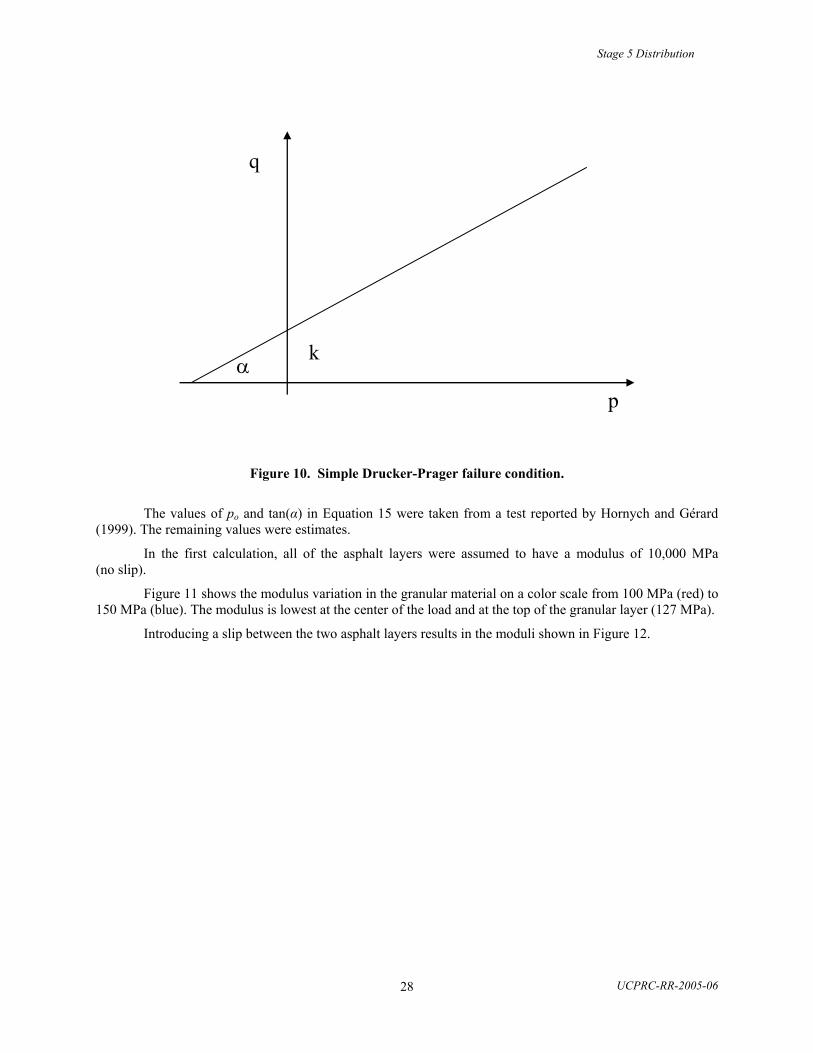
Stage 5 Distribution
UCPRC-RR-2005-06 28
Figure 10. Simple Drucker-Prager failure condition.
The values of po and tan(α) in Equation 15 were taken from a test reported by Hornych and Gérard (1999). The remaining values were estimates.
In the first calculation, all of the asphalt layers were assumed to have a modulus of 10,000 MPa (no slip).
Figure 11 shows the modulus variation in the granular material on a color scale from 100 MPa (red) to 150 MPa (blue). The modulus is lowest at the center of the load and at the top of the granular layer (127 MPa).
Introducing a slip between the two asphalt layers results in the moduli shown in Figure 12.
p
q
α k

Stage 5 Distribution
UCPRC-RR-2005-06 29
Figure 11. EAC 10,000 MPa, no slip, 40 kN load.

Stage 5 Distribution
UCPRC-RR-2005-06 30
Figure 12. EAC 10,000 MPa, slip, 40 kN.
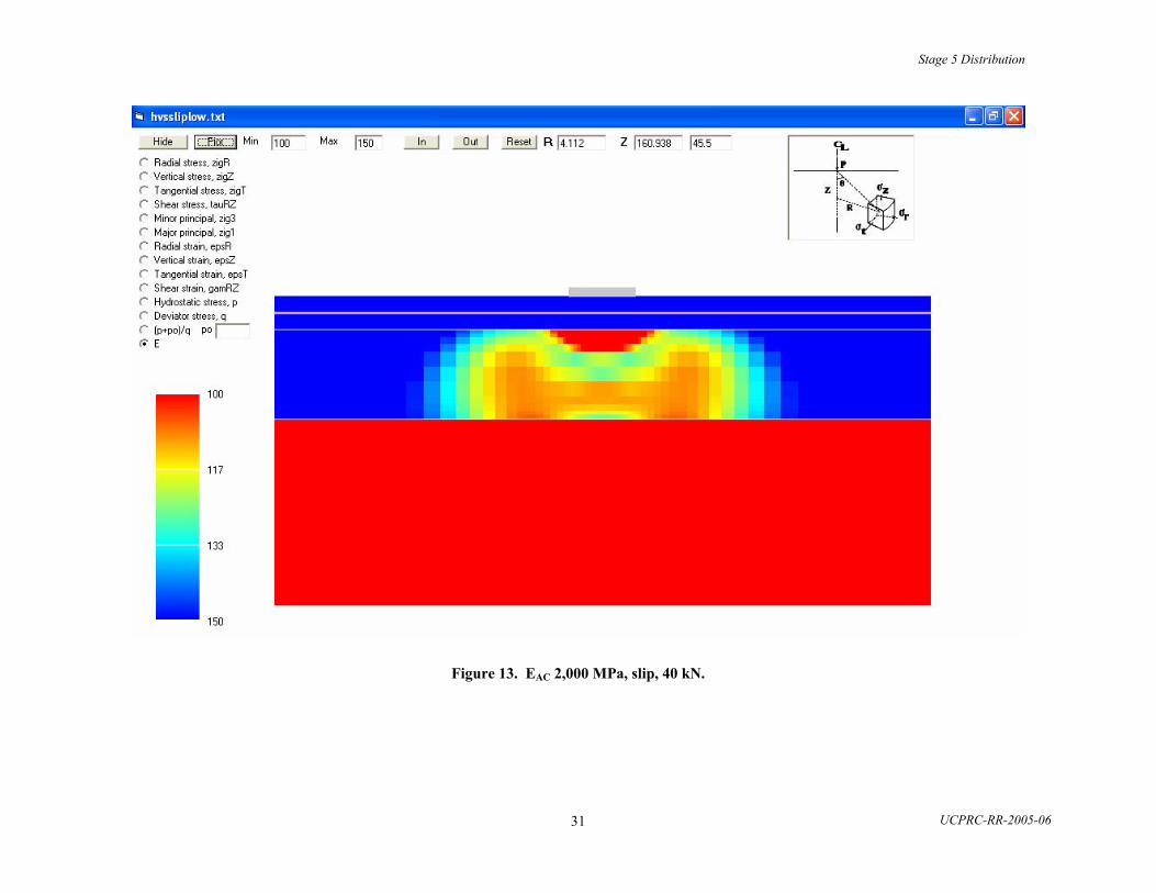
Stage 5 Distribution
UCPRC-RR-2005-06 31
Figure 13. EAC 2,000 MPa, slip, 40 kN.

Stage 5 Distribution
UCPRC-RR-2005-06 32
The modulus of the granular material decreases at the center of the load, indicating that the effect of the deviator stress is more important than the effect of the confining stress.
Decreasing the modulus of the two asphalt layers to 2,000 MPa results in an even lower modulus of the granular layer, as seen in Figure 13. This decrease in modulus of the granular layer with development of slip and with a decrease in the modulus of the asphalt layers is in good agreement with the observed changes during HVS and FWD testing.
Increasing the load from 40 kN to 100 kN, however, causes a further decrease in the modulus of the granular layer, as shown in Figure 14. This is contrary to the change observed during HVS testing, where an increase in the load from 40 kN to 100 kN resulted in an increase in the modulus of the granular layers.
Therefore it is doubtful whether the changes in the modulus of the granular layers can be explained solely by the stress dependence of the material. It may be necessary to include the particulate nature of the material, for example, by using the Distinct Element Method, an expample of which was given by Ulliditz (2002). The Distinct Element Method was used with a 1000×2000 mm “box” filled with 3,662 particles. The particles had been compacted in two layers to a thickness of 830 mm for the lower layer and 100 mm for the upper layer. Particle size distribution and angularities were different for the two layers. In the upper layer, cohesion is assumed between the particles, as well as a permissible tensile force (of 20 N at each contact point). In Figure 15, the vectors from the centers of the particles show the displacement during the first 8 msec of loading on a 150-mm plate at the surface of the sample. All contacts were intact at this low load.

Stage 5 Distribution
UCPRC-RR-2005-06 33
Figure 14. EAC 2,000 MPa, slip, 100 kN load.

Stage 5 Distribution
UCPRC-RR-2005-06 34
The displacement field is quite different from what would have been obtained in an elastic solid, with a great deal of particle rotation and uplift away from the load. Figure 16 shows an example from a Finite Element calculation, with the same proportions and the same center-line deflection. In the elastic solid most of the displacement is downward with only a slight rotation away from the load.
Figure 15. Displacement field in particulate sample.
This suggests that the stiffness of the upper layer may be important to the displacement of the granular material and thus to the (apparent) stiffness of the material. The upper layer acts as a plate controlling the upward and outward rotation of the particles away from the load. The Discrete Element Method analysis suggests that a stiffer plate (the asphalt layers) over the granular layers would tend to decrease the displacements of the granular particles, thus increasing their effective stiffness. HVS and FWD tests have indicated that the granular layer stiffness decreases as the asphalt layers stiffness decreases, whether that decrease is temporary (caused by temperature change) or permanent (caused by fatigue damage).
However, in order to simulate HVS testing, it is essential that deflections be predicted correctly. To do this, changes in moduli must be modeled. A procedure for doing so was developed and used for this report. The procedure, based on the observations discussed earlier, is described below.
The stiffness reduction of the unbound layers was assumed to be a fraction of the decrease in the stiffness of the layers above the one under consideration, this fraction is referred to as the “stiffness factor” in this report. The decrease in stiffness of the unbound layers was treated as “apparent” (and temporary) damage (i.e., it would disappear if the stiffness of the layers above recovered, such as in the case of changing temperature). If the reference stiffness of the layers above a certain layer is Sref and the present stiffness is S, then the apparent damage is calculated as:
factorStiffnessSSdamageApparent
ref×⎟
⎠
⎞⎜⎝
⎛ −= 1 (17)

Stage 5 Distribution
UCPRC-RR-2005-06 35
0
100
200
300
400
500
600
700
800
900
-1000 -800 -600 -400 -200 0 200 400 600 800 1000Distance from centre, mm
Dep
th, m
m
Figure 16. Displacement field in elastic solid (FEM).
The moduli of the unbound materials were calculated from the equation:
( )( )31
1
3
,/11
⎟⎟⎠
⎞⎜⎜⎝
⎛×=
×−−×=
∑−n
ii
ref
EhS
withfactorStiffnessSSEoE (18)
where Eo is the modulus (of layer n) when the combined stiffness of the layers above (S) is equal to the reference stiffness (Sref).
A reference stiffness of 35003 N/mm was used for all unbound materials. (For practical reasons, the input to the program is the cube root of the reference stiffness, or, in this case, 3500.) For the stiffness calculation in Equation (18), the layers are assumed to be fully bonded. If two layers are debonded, the combined stiffness is calculated as h1
3 × E1 + h23 × E2. A full bond is assumed if the slip value is more than
100; a full slip is assumed when the value is less than 0.01. A logarithmic interpolation is used between these two values.
FWD tests were carried out on September 29, 1995, in the lines of the HVS test sections of Goal 1 (with the exception of the Section 500RF test area where testing was ongoing), with asphalt temperatures of 20–22ºC. Layer moduli were backcalculated using Elmod5 software and the following layer thicknesses were assumed:

Stage 5 Distribution
UCPRC-RR-2005-06 36
Table 8. Layer Thicknesses Used for FWD Backcalculation
HVS Test Section Layer 1 Layer 2
500RF 225 mm 320 mm
501RF 150 mm 490 mm
502CT 225 mm 400 mm
503RF 150 mm 580 mm
All of the asphalt bound layers (including ATPB) were combined into Layer 1 and the two granular
layers into Layer 2. Drop 2 of the FWD tests, with a peak contact stress of about 0.6 MPa, was used.
AB + ASB undrained y = 205.42x + 210.31R2 = 0.1391
0
50
100
150
200
250
300
350
400
450
0 0.1 0.2 0.3 0.4 0.5 0.6 0.7
Stiffness/Reference stiffness
Mod
ulus
, MPa
Figure 17. Modulus of Layer 2 as a function of the stiffness of the asphalt layers, for the undrained
sections.

Stage 5 Distribution
UCPRC-RR-2005-06 37
AB + ASB drained y = 116.2x + 152.64R2 = 0.2899
0
50
100
150
200
250
300
350
400
450
500
0 0.2 0.4 0.6 0.8 1 1.2 1.4 1.6 1.8
Stiffness/Reference stiffness
Mod
ulus
, MPa
Figure 18. Modulus of Layer 2 as a function of the stiffness of the asphalt layers, for the drained
sections.
Subgrade (drained and undrained) y = 23.775x + 88.724R2 = 0.5155
0
50
100
150
200
250
300
0 1 2 3 4 5 6 7 8
Stiffness/Reference stiffness
Mod
ulus
, MPa
Figure 19. Modulus of subgrade as a function of the stiffness of the pavement layers.

Stage 5 Distribution
UCPRC-RR-2005-06 38
In Figure 17 through Figure 19, the moduli of the unbound layers are shown as functions of the stiffness ratio of the layers above. The correlation between stiffness ratio and modulus is not very good, but if the best fitting lines are used anyway, the stiffness parameters shown in Table 9 result.
Table 9. Moduli Parameters from FWD
Layer Eo, MPa Stiffness Factor
AB + ASB undrained 416 0.49
AB + ASB drained 269 0.43
Subgrade 112 0.21
Based on the calibration using Section 501RF the parameters shown in Table 10 were chosen:
Table 10. Moduli Parameters from Calibration to MDD Deflections
Material Eo, MPa Stiffness Factor
Aggregate base 165 0.4
Aggregate subbase 115 0.3
Subgrade 60 0.2
These values were used for all of the tests of Goals 1, 3, and 5, except for the subgrade of Section 502CT (and the corresponding overlay section, 515RF), where a value of 102 MPa was used in order to get a more correct initial subgrade deflection. In the simulations with full bond, factors of 0.55, 0.45, and 0.3 were used to compensate for the lack of slip. This was to ensure correct deflections during the simulation, where only the permanent deformation of the asphalt was determined.
The initial moduli used in the HVS simulations for Goal 1 and Goal 3 appear in Table 11. The moduli correspond to a 40 kN wheel load, a loading time of 0.015 sec., and a temperature of 20ºC. The moduli are given in MPa.

Stage 5 Distribution
UCPRC-RR-2005-06 39
Table 11. Initial Moduli Used in HVS Simulations (MPa)
Section Overlay AC top AC bottom
ATPB AB ASB Subgrade
501RF 9038 11173 149 161 103
503RF 9038 11173 165 182 134
500RF 9038 11173 1144 199 186 105
502CT 9038 11173 1144 197 184 199
517RF 7653 1968 2733 162 177 113
518RF 4755 1968 2733 133 140 102
514RF 7653 2881 4997 807 242 227 125
515RF 4755 2881 4997 808 175 164 178
Table 12 gives a summary of the moduli determined by different methods. The range of moduli is given in MPa.
Table 12. Summary of Moduli (MPa)
Material Triaxial FWD MDD
AB-ASB 140-430 200-400 120-240
Subgrade 55-100 100-150 100-200
It may be noted that asphalt moduli from the master curve developed from backcalculated FWD deflections were lower than those from the master curve developed from measured moduli in frequency sweep tests, after the minimum modulus of the frequency sweep-derived master curve had been set at a value of 200 MPa (note see Figure 224 for similar occurance with the Goal 9 master curve for the underlying asphalt concrete). The larger asphalt moduli from the frequency sweep tests were used when backcalculating the moduli of the unbound materials using MDD deflections. The unbound layers’ moduli backcalculated from the MDD deflections would have been larger if the FWD asphalt moduli had been used with the MDD deflections instead of the frequency sweep moduli.
1.5.3 Influence of Load Level
During testing, MDD deflections were measured under different wheel loads. This showed that the moduli of the unbound layers were not constant; they changed with the load level. Because of the effect of the stiffness of the layers above the unbound layers, this non-linearity could not be treated as a function of the stress condition in the material (because of the influence of the stiffness of the above layers). Instead, it had to be treated as a function of the load level. The modulus at load level P was calculated as:

Stage 5 Distribution
UCPRC-RR-2005-06 40
kNP EkN
PE 4040×⎟⎟
⎠
⎞⎜⎜⎝
⎛=
α (19)
The power α was 0.6 for the granular layers and -0.3 for the subgrade. Both are typical values for granular and cohesive materials, respectively.
The permanent deformation of the materials is a function of the resilient pavement response but, with the models used here, the response is independent of the permanent deformation. The parameters controlling resilient response can, therefore, be determined without considering permanent deformations, as was done in the sections above. Once the calculated response appears to be correct, the parameters controlling the permanent deformations may be calibrated.
1.6 Permanent Deformation
1.6.1 Asphalt
A shear-based approach, developed by Deacon et al. (2002), for predicting rutting of the asphalt layer was used in a first attempt. Rutting in the asphalt is assumed to be controlled by shear deformation. The computed values of shear stress, τ, and elastic shear strain, γe, at a depth of 50 mm beneath the edge of the tire are used for the rutting estimates.
Rutting in the AC layer due to the shear deformation is determined from the following:
( )γα γτβγ e
ref
iAC resp
MNAKmmrd ×⎟⎟⎠
⎞⎜⎜⎝
⎛ ××=×= exp (20)
where ACrd mm is the vertical rut depth in the asphalt concrete γi = permanent (inelastic) shear strain at 50 mm depth, τ =shear stress determined at this depth using elastic analysis, γe = corresponding elastic shear strain (m/m), K is a value relating permanent shear strain to rut depth (mm), and A, α, β, respref, and γ are constants.
The purpose of respref is to make the right side of the equation unitless. Atmospheric pressure (0.1 MPa) was selected as the value for respref , and γ was assumed to be 1. Two Repeated Simple Shear Tests at Constant Height (RSST-CH) were available for the top layer of Goal 1 (for the initial simulations), both at 40ºC and at a shear stress of approximately 70 kPa. From these tests A/K = 49.3 and α = 0.208 could be derived. The constant β was set at 1.03 based on the experiments by Deacon et al. (2002). The research team determined A/K and α by importing the results of the RSST-CH (number of load applications, shear stress, resilient shear strain, temperature, and permanent shear strain) into a spreadsheet. The tests were then modeled using the right part of Equation (20) (the permanent strain part). The RMS difference between the measured and calculated permanent strain was calculated. Excel’s “Solver” was used to minimize this difference by changing A/K and α.
The constant A was determined from a simulation of Section 501RF with full friction at the first interface. The fatigue shift factor and the stiffness factors for the unbound layers were adjusted, as mentioned above, in order to get the correct resilient deflections during the full test period. In determining A the first 500,000 load applications were used, as the measured data showed an unexplained 1-mm increase in the permanent deformation of the AC layers from 550,000 to 600,000 load repetitions.
For Goal 1, A was found to be about 400, which corresponded to a K value of 8.1.
It should be noted that the modulus of the asphalt decreased due to damage during the test. In the initial attempt, the shear stress and shear strain were calculated using the modulus of the damaged material. A

Stage 5 Distribution
UCPRC-RR-2005-06 41
decrease in modulus caused by damage could have influenced the permanent deformation in the AC differently from a similar modulus decrease due to an increase in temperature.
The parameters used in the first set of simulations and in the simulation of the underlying pavement of Goal 9 are given in Table 13.
Table 13. Parameters Used in Equation 20
Test Material A α
Goal 1 DGAC1 400 0.208
DGAC3 700 0.208 Goal 3,
20ºC ARHM 400 0.208
DGAC1 700 0.208
DGAC3 1500 0.17
Goal 3,
45ºC
ARHM 1500 0.17
DGAC3 700 0.208 Goal 5
ARHM 400 0.208
In general the parameters gave a good fit to the measured permanent deformations, although there were problems with thin overlays, less than 50 mm thick, where no permanent deformation was determined.
As can be seen, the parameters used are not totally consistent. Because of the problem with thin layers the approach was modified using additional RSST-CH test data as explained below.
Figure 20 shows the results of ten RSST-CH for field mix, field compacted (FMFC) specimens from the dense-graded asphalt concrete (DGAC) of Goal 3. The air-void content for these specimens was close to 5.5 percent. Testing was done at 40ºC, 50ºC, and 60ºC. The applied shear stress was reasonably constant at 70 kPa.
The value of α in Equation (20) corresponds to the slope of the curves in Figure 20. It is quite evident that the slope is not constant. Even if only the values above 100 load applications are included, there is still a considerable variation, both with the number of load applications for each curve and between the curves.
Two approaches were tried in order to get a better relationship between the plastic shear strain and the number of load applications: a Weibull function and a Gamma function.

Stage 5 Distribution
UCPRC-RR-2005-06 42
Goal 3 DGAC FMFC AV5.5
0.0001
0.001
0.01
0.1
1 10 100 1000 10000 100000
Number of loads
Plas
tic s
trai
n
60_6760_6860_6850_7050_6550_6740_7340_7440_7240_73
Figure 20. Results of RSST-CH tests. [Note: FMFC indicates field-mixed field compacted specimen taken by coring the pavement. AV5.5 indicates cores with approximately 5.5 percent air-voids. Each title
in the legend indicates the RSST-CH test temperature (40, 50, or 60 °C) and average shear stress (MPa).]

Stage 5 Distribution
UCPRC-RR-2005-06 43
Weibull function:
The Weibull function may be written as:
( )αNAS ×−= exp (21) where S is the normalized plastic shear strains as defined by Equation 22 in terms of the elastic and
permanent (inelastic) shear strains, N is the load repetitions, A and α are constants determined from the test.
To use a Weibull function S may be calculated from the plastic shear strain, “normalized” by inclusion of the term γref, from:
refe
ref
iS
γγττβ
γ
××⎟⎟⎠
⎞⎜⎜⎝
⎛ ×−=
exp1 (22)
The value of the constant γref must be selected so that S will never get below zero. A value of 1000 was used here.
Equation (21) may be rewritten as:
( )( ) ( ) ( )NAS lnlnlnln ×+=− α (23)
The data from the Goal 3 tests in Figure 20 have been plotted on this format in Figure 21. Although there is a certain amount of scatter, the normalization seems to collapse the tests reasonably well.
Figure 22 shows the average values of the curves in Figure 21 as well as the best fitting straight line. Although the coefficient of correlation is quite high the fit is not very good and the slope of the line keeps changing with increasing number of loads. This is important as the maximum number of load applications during the RSST-CH tests is about 40,000, whereas the number of load applications during HVS testing (or on in situ roads) may be much larger.

Stage 5 Distribution
UCPRC-RR-2005-06 44
Goal 3 DGAC FMFC AV5.5
-8
-7.5
-7
-6.5
-6
-5.5
-5
-4.5
-4
-3.5
-3
0 2 4 6 8 10 12
ln(N)
ln(-l
n(S)
)
Figure 21. Normalized plastic strain versus number of load repetitions. (Note: legend is the same as in Figure 20).

Stage 5 Distribution
UCPRC-RR-2005-06 45
Goal 3 DGAC FMFC AV5.5 Average
y = 0.2941x - 6.681R2 = 0.9099
-8
-7.5
-7
-6.5
-6
-5.5
-5
-4.5
-4
-3.5
-3
0 2 4 6 8 10 12
ln(N)
ln(-l
n(S)
)
Figure 22. Average values for Figure 21 curves.
A relationship of the format:
eref
iNA γ
ττβγγ
α×⎟
⎟⎠
⎞⎜⎜⎝
⎛ ××
⎟⎟
⎠
⎞
⎜⎜
⎝
⎛
⎪⎭
⎪⎬⎫
⎪⎩
⎪⎨⎧
⎟⎠⎞⎜
⎝⎛−×= expexp (24)
was also attempted. This format is similar to the format used for unbound materials in the NCHRP 1-37A report. It did not improve the fit.
Gamma function:
An alternative to fit the data was a gamma function of the format:
( )Nxandy
xxAy
eref
iln,
expln
1exp1
=
⎟⎟⎟⎟⎟
⎠
⎞
⎜⎜⎜⎜⎜
⎝
⎛
×⎟⎟⎠
⎞⎜⎜⎝
⎛ ×=
⎥⎦⎤
⎢⎣⎡ ⎟
⎠⎞⎜
⎝⎛ +×⎟
⎠⎞⎜
⎝⎛−−×+=
γττβ
γ
γγα
(25)

Stage 5 Distribution
UCPRC-RR-2005-06 46
The plastic strain may be calculated from:
( ) ( ) eref
i NNA γττβ
γγαγ ×⎟⎟⎠
⎞⎜⎜⎝
⎛ ××⎟⎠⎞
⎜⎝⎛
⎥⎦⎤
⎢⎣⎡ ⎟
⎠⎞⎜
⎝⎛ +×⎟
⎠⎞⎜
⎝⎛−−×+= expln1lnexp1exp (26)
To use the time-hardening method in CalME, the apparent N must be calculated at the beginning of each time increment. The “apparent N” is the equivalent number of load repetitions at the temperature of the next time increment to reach the permanent shear strain calculated at the temperature of the current time increment. This cannot be done directly, but requires an iterative procedure, for example using the equation:
( )
( ) α
γττβ
γ
γ
γ
A
N
N eref
i−
⎟⎟⎟⎟⎟
⎠
⎞
⎜⎜⎜⎜⎜
⎝
⎛
×⎟⎟⎠
⎞⎜⎜⎝
⎛ ×
−=⎟⎠⎞⎜
⎝⎛
+ expln
1lnexp
ln1 (27)
The following parameters were obtained:
• A = -0.568
• α = 4.208
• γ = 2.472
The RMS value on the ln (Normalized strain) was 0.30.
Figure 23 shows that the Gamma function fits the measured data quite well. Therefore, it was selected for the rest of this study.
Goal 3 DGAC FMFC AV5.5
-2
-1
0
1
2
3
4
0 2 4 6 8 10 12
ln(Number of loads)
ln(N
orm
aliz
ed S
trai
n)
Gamma fit
Figure 23. Best fitting Gamma function. (Note: legend is the same as in Figure 20 and Figure 21.

Stage 5 Distribution
UCPRC-RR-2005-06 47
For the Goal 1 DGAC mixes, all five tests (from the top layer and the bottom layer, which were not very different) were used to determine the parameters of the Gamma function:
• A = -1.316
• α = 5.218
• γ = 2.860
The RMS was 0.16.
For the ARHM, with an air-void content of 10 percent, of Goal 3 the following parameters were obtained:
• A = -0.506
• α = 4.703
• γ = 2.572
The RMS was 0.36.
The permanent deformation was still assumed to be a constant times the permanent shear strain, but in order to include permanent deformation in overlays less than 50 mm thick, the permanent deformations were prorated over the layers within a depth of 100 mm from the surface.
The shear stress, τ, was still calculated at a depth of 50 mm at the edge of a tire and by using the moduli of the pavement’s individual layers. For each layer the elastic shear strain was then determined from:
( )ντγ
+=
1/Ee (28)
Where γe is the elastic shear strain, τ is the shear stress, ν is Poisson’s ratio, and E is the modulus of the layer considered, including any reduction in modulus caused by
fatigue damage (also for the Goal 3 rutting tests). The permanent shear strain in the layer was determined from Equation 26, and the permanent
deformation was obtained by multiplying the permanent shear strain by the thickness of the layer (in mm) and by a constant, K.
A value of 0.25 was used for K for all materials, except the Goal 1 DGAC, which would either be tested at a relatively low temperature of about 20ºC or would have been in place several years before being tested. Instead, a K value of 0.08 was used for the DGAC from Goal 1.
The permanent deformations shown in the simulations that appear later in this report for the individual HVS test sections were calculated by using the Gamma function and prorating the deformation, except for Goal 9 where the power function was used.
1.6.2 Unbound Materials
Permanent deformation, dp, of the unbound materials is based on the vertical resilient strain at the top of the layer, με, and on the modulus of the material, E:
,ref ref
Edp mm A MNE
β γ
α μεμε
⎛ ⎞ ⎛ ⎞= × × ×⎜ ⎟ ⎜ ⎟⎜ ⎟ ⎜ ⎟
⎝ ⎠ ⎝ ⎠ (29)

Stage 5 Distribution
UCPRC-RR-2005-06 48
The input parameters used for the subgrade are given in the second column of Figure 24. The parameters are based on a series of full-scale tests in the Danish Road Testing Machine, with a subgrade of Danish "Moraine Clay," which is classified as a “clayey, silty sand” [AASHTO classification A-4(0)] (Ullidtz 2005).
Figure 24. Input parameters for permanent deformation (rutting) of subgrade in second column.
The same parameters were used for the two granular layers, except that the value of A was reduced to 0.8.
The permanent compression of the unbound layers is rather small, and the scatter between different tests — and even between different MDDs within a single test — is quite large. Therefore, it is difficult to draw any definitive conclusions. However, the model and parameters given above appear to predict the permanent deformation of the unbound layers reasonably well.
1.7 Reflection Cracking
Reflection cracking damage was calculated using the method developed by Wu (2005). In this method the tensile strain at the bottom of the overlay is estimated using a regression equation. The calculated tensile strain at the bottom of the overlay is used with the fatigue equation described previously to calculate damage in the asphalt layers.
The regression equation for tensile strain at the bottom of the overlay is based on many two-dimensional (2D) Finite Element analyses of overlay structures from a parametric study shown in Table 14. Figure 25 compares the predicted 2D strain from the regression equation against the calculated strain.

Stage 5 Distribution
UCPRC-RR-2005-06 49
Table 14. AC on AC, 2D Structural Parameter Combinations
Name Description Unit Variations Ea Stiffness of Overlay MPa 4000, 6000, 8000, 10000, 12000 Ha Thickness of Overlay mm 50, 75, 100, 150, 200, 250 Eu Stiffness of the Underlayer MPa 3000, 5000, 7000 Hu Thickness of the Underlayer mm 100, 200, 300 Eb Stiffness of the Base/Sub-base MPa 150, 300, 450 Es Stiffness of the Subgrade Ma 100, 200 LS Crack Spacing mm 55, 110, 220, 440 Total number of runs: 6,480
The variables in Table 14 are normalized for the parametric study so that they are close to 1.0 and dimensionless:
aE = /Ea 10000 MPa, SL = /SL 200 mm, aH = /Ha 100 mm, uH = /Hu 200 mm,
uE = /Eu 5000 MPa, bE = /Eb 300 MPa, sE = /Es 200 MPa.
0
100
200
300
400
500
600
700
800
900
1000
0 100 200 300 400 500 600 700 800 900 1000
Calculated Strain (με)
Fitt
ed S
trai
n ( μ
ε)
Fitted ValuesLine of Equality
Figure 25. Comparison of fitted vs. calculated strain for AC-on-AC overlay, 2D.
The 2D strains are converted to three-dimensional (3D) strains using another regression equation based on hundreds of Finite Element analyses from the same factorial used for the 2D analysis.

Stage 5 Distribution
UCPRC-RR-2005-06 50
The 2D strain function is:
)ˆ1)(ˆ1)(ˆexp()]ˆln(0.1[ˆˆˆ43212
321uuassbaD EbHbHbLbEEE ++−+= −−− βββαε (30)
with parameters α = 226.53, β1 = 0.73722, β2 = 0.26455, β3= 0.16295, b = 0.15272, b = 0.23069, b = -0.13011, b = 0.46881.
Figure 25 shows a plot of the fitted versus the calculated 2D strains for AC-on-AC overlays.
For the 2D to 3D transformation ε3D = γ·ε2D and the coefficient γ can be expressed as:
sLbbEbuHbuEbaHbaEbb ˆˆˆˆˆˆ6543210 ++++++=γ (31)
with parameters b0 = 0.61594, b1= 0.32834, b2 = 0.27215, b3 = 0.070884, b4 = 0.054061, b5 = 0.13092, b6 = 0.13633.
A crack spacing of 200 mm was assumed in the Goal 3 simulations based on the crack spacings observed at the end of the Goal 1 tests.
2.0 GOAL 1 CRACKING TEST SIMULATIONS
2.1 Goal 1 Resilient Deformations
The pavement response was calculated for each hour of the HVS test, and it was assumed that each HVS loading sequence was evenly distributed over time (with an almost constant temperature this has little significance). The load was placed at five transverse positions across the width of the loaded area, which was 1,000 mm for all tests, the width of the wander pattern used for the HVS dual wheel. Damage to the asphalt for each wheel position was accumulated using the “time hardening” method, i.e., by first calculating the number of load applications required to cause the present damage, given the present pavement response and conditions, then by calculating the damage that would be caused by that number of load applications plus the number of loads applied at the wheel position during the hour under consideration.
Damage to the asphalt was based on the minor principal strain (compression as positive) at the bottom of the lowest asphalt layer (including the ATPB as an asphalt layer, as long as the damage of this layer was less than 0.9), when the layers were bonded. After debonding, the strain at the bottom of the top layer was used to calculate the damage of the top layer. Apparent damage to the unbound layers was calculated using the damage to the asphalt layers, the degree of bonding between asphalt layers, and the apparent damage to any unbound layer above the layer under consideration. Temperature variation in the asphalt layers also affects the apparent damage of the unbound layers.
The calculated damage (and apparent damage) were stored in the Performance table of the DesignData.mdb and for possible later use to calculate deflection at the MDD modules (or any other response value).
2.1.1 Section 501RF Resilient Deflections (Undrained)
The first calibration was done using Test Section 501RF. This section had no ATPB layer and the test was relatively short, lasting for a little more than three months. The MDDs also appeared to function correctly.
The following figures show the deflection of the top MDD modules, the resilient compression of the pavement layers (which is the difference in deflection between two MDD modules), and the deflection at the top of the subgrade. They are first shown for a wheel load of 40 kN, then for a wheel load of 100 kN. All

Stage 5 Distribution
UCPRC-RR-2005-06 51
simulations were done with the stiffness parameters for the unbound materials given in Table 10. The shift factor for asphalt fatigue was 3 for all the asphalt layers, i.e., it took three HVS loads at a given strain, modulus, and temperature to produce the same damage as one load in the laboratory bending beam test. Slip was assumed to have been fully developed after 2 MESAL (million ESAL, calculated using the Caltrans 4.2 Exponent, which corresponds to approximately 200,000 load repetitions).
The first visible cracking was recorded at approximately 550,000 load repetitions.
Figure 26. Section 501RF pavement structure.
In the figures below, measured deflections are indicated by an M, similarly followed by a number revealing MDD module depth, and calculated deflections are indicated by the letter C, again followed by a number denoting depth. For compression of a layer between two modules, the depths of the two modules are given, with M and C indicating measured and calculated values, respectively.
The following legend is used in Figure 28 and all subsequent figures of this type. Each item in the numbered list of explanations below appears boxed in Figure 28:
1. The wheel load under which the deflections were measured and calculated.
2. The MDDs that were used in the measurement. In the above case, the first measured value is from MDD stack number 1, module number 1, and the second measured value is from MDD stack number 2, module number 1 (the modules are counted from the top, so for both MDDs the top modules were used in the figure).
3. The legend for the first measured value (M for measured), which was at depth 0 mm (i.e., on the surface, for the second measured value, shown in the legend as M137, the depth was 137 mm). In figures where the measured difference in deflection or deformation between two modules is plotted, it will be shown as M0-640, which would indicate the measured deflection or deformation between the depths of 0 and 640 mm.
4. The legend for the first calculated value (C for calculated), which will be at the same depth as the first measured value (i.e., C0 is the calculated deflection on the surface; for the second calculated value, shown in the legend as C137, the depth was 137 mm). In figures where the calculated difference in deflection or deformation between two modules is plotted, it will be shown as C0-640, which would indicate the calculated deflection or deformation between the depths of 0 and 640 mm.

Stage 5 Distribution
UCPRC-RR-2005-06 52
0
5
10
15
20
25
30
0 200000 400000 600000 800000 1000000 1200000 1400000
Loads
Tem
pera
ture
(ºC
)
Outside Air 0mm 50mm 137mm 175mm
40kN (20ºC) 80kN (20ºC)
100kN (20ºC)
Figure 27. Section 501RF temperatures during testing.
Figure 28. Section 501RF 40 kN top modules deflection.

Stage 5 Distribution
UCPRC-RR-2005-06 53
Figure 29. Section 501 RF 40 kN resilient compression of pavement layers.
Figure 30. Section 501RF 40 kN deflection of subgrade.

Stage 5 Distribution
UCPRC-RR-2005-06 54
Figure 31. Section 501RF 100 kN deflection of top modules.
Figure 32. Section 501RF 100 kN resilient compression of pavement layers.
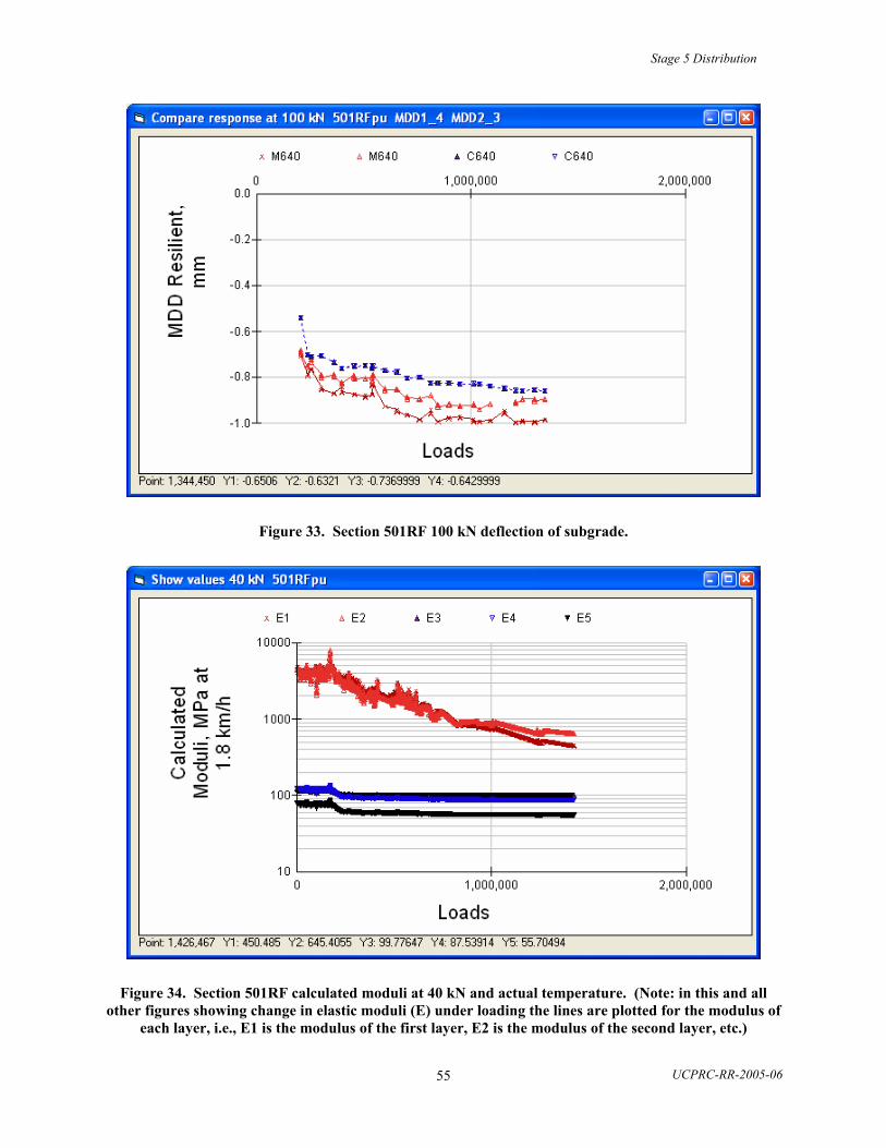
Stage 5 Distribution
UCPRC-RR-2005-06 55
Figure 33. Section 501RF 100 kN deflection of subgrade.
Figure 34. Section 501RF calculated moduli at 40 kN and actual temperature. (Note: in this and all other figures showing change in elastic moduli (E) under loading the lines are plotted for the modulus of
each layer, i.e., E1 is the modulus of the first layer, E2 is the modulus of the second layer, etc.)

Stage 5 Distribution
UCPRC-RR-2005-06 56
2.1.2 Section 503RF Resilient Deflections (Undrained)
The pavement structure for Section 503RF is shown in Figure 35. The first visible cracking was recorded at approximately 650,000 load repetitions.
Figure 35. Section 503RF pavement structure.
0
5
10
15
20
25
30
35
0 200000 400000 600000 800000 1000000 1200000 1400000 1600000 1800000 2000000
Loads
Tem
pera
ture
(ºC
)
Outside Air 0mm 50mm 90mm 137mm
40kN (20ºC) 80kN (20ºC)
100kN (20ºC)
Figure 36. Section 503RF temperatures during testing.

Stage 5 Distribution
UCPRC-RR-2005-06 57
Figure 37. Section 503RF 40 kN deflection of top modules.
One of the MDDs on the subgrade only functioned for part of the test.
Figure 38. Section 503RF 40 kN compression of pavement layers.

Stage 5 Distribution
UCPRC-RR-2005-06 58
Figure 39. Section 503RF 40 kN deflection of subgrade.
Figure 40. Section 503RF 100 kN deflection of top modules.
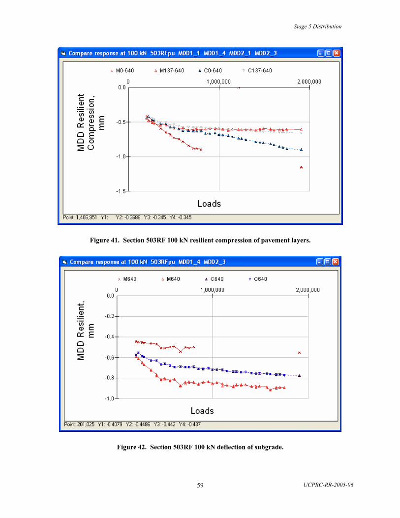
Stage 5 Distribution
UCPRC-RR-2005-06 59
Figure 41. Section 503RF 100 kN resilient compression of pavement layers.
Figure 42. Section 503RF 100 kN deflection of subgrade.

Stage 5 Distribution
UCPRC-RR-2005-06 60
Figure 43. Section 503RF calculated layer moduli at 40 kN and actual temperature.
2.1.3 Section 500RF Resilient Deflections (Drained)
The pavement structure for Section 500RF is shown in Figure 44. The first visible cracking was recorded at approximately 650,000 load repetitions.
Figure 44. Section 500RF pavement structure.

Stage 5 Distribution
UCPRC-RR-2005-06 61
0
5
10
15
20
25
30
35
40
0 500000 1000000 1500000 2000000 2500000
Loads
Tem
pera
ture
(ºC
)
Outside Air 0mm 70mm 137mm 175mm
40kN 80kN 100kN
Figure 45. Section 500RF temperatures during testing.
Figure 46. Section 500RF 40 kN deflection of top modules.

Stage 5 Distribution
UCPRC-RR-2005-06 62
Figure 47. Section 500RF 40 kN resilient compression of pavement layers.
Figure 48. Section 500RF 40 kN deflection of subgrade.
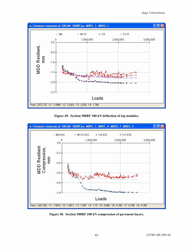
Stage 5 Distribution
UCPRC-RR-2005-06 63
Figure 49. Section 500RF 100 kN deflection of top modules.
Figure 50. Section 500RF 100 kN compression of pavement layers.

Stage 5 Distribution
UCPRC-RR-2005-06 64
Figure 51. Section 500RF 100 kN deflection of subgrade.
Figure 52. Section 500RF calculated moduli at 40 kN and actual temperature.

Stage 5 Distribution
UCPRC-RR-2005-06 65
2.1.4 Section 502CT Resilient Deflections (Drained)
The pavement structure for Section 502CT is shown in Figure 53. Temperature data is missing from Section 502CT. For all layers throughout the test, 20ºC was used. The first visible cracking was recorded at approximately 1,310,000 load repetitions.
Figure 53. Section 502CT pavement structure.
Figure 54. Section 502CT 40 kN deflection on top of AC.

Stage 5 Distribution
UCPRC-RR-2005-06 66
Figure 55. Section 502CT 40 kN compression of pavement layers.
Figure 56. Section 502CT 40 kN deflection of subgrade.

Stage 5 Distribution
UCPRC-RR-2005-06 67
Figure 57. Section 502CT 100 kN deflection at top of AC.
Figure 58. Section 502CT 100 kN resilient compression of pavement layers.

Stage 5 Distribution
UCPRC-RR-2005-06 68
Figure 59. Section 502CT 100 kN deflection of subgrade.
Figure 60. Section 502CT calculated moduli at 40 kN and 20ºC.

Stage 5 Distribution
UCPRC-RR-2005-06 69
Given the scatter in the measured data, the agreement between measured and calculated deflections and compressions could probably not have been much better. Although this does not guarantee that the strains calculated to determine the damage in the asphalt are correct (as was noted in the Introduction) or that the calculated moduli throughout the HVS test are in accordance with the actual moduli, it is a strong indication that this is the case.
It should be recalled, however, that a number of assumptions have been made, and it is possible that different assumptions could result in equally good or better agreement between measured and calculated deflections.
2.2 Visual Cracking Versus Damage of the Top Asphalt Layer, Goal 1
Cracking at the pavement surface was recorded in m/m2. In Figure 61, the observed cracking is shown versus the relative decrease in the modulus of the top asphalt layer, assuming an intact modulus of 5,669 MPa at a temperature of 20ºC, a wheel speed of 7.6 km/h, and a minimum modulus of 200 MPa.
There is a clear difference between the drained and the undrained pavement sections. For the undrained sections (501RF and 503RF) the first visual cracking appears when the modulus has dropped by about 50–60 percent, whereas the corresponding drop in modulus for the drained sections is about 70–80 percent.
For all four test sections, the deflection under a 40-kN load — measured with the top MDD modules — had doubled before any surface cracking was observed. This also indicates that the pavement structures underwent considerable damage before any cracking was observed.
Visual cracking versus decrease in modulus
0
2
4
6
8
10
12
0 0.2 0.4 0.6 0.8 1
dE/Ei
Cra
ckin
g, m
/m2
500RF drained501RF undrained502CT drained503RF undrained
Figure 61. Cracking versus relative decrease in modulus of top AC layer for Goal 1.

Stage 5 Distribution
UCPRC-RR-2005-06 70
Cracking versus relative deflection
0
2
4
6
8
10
12
1 1.5 2 2.5 3 3.5
Deflection/initial deflection
Cra
ckin
g m
/m2
500RF drained501RF undrained502CT drained503RF undrained
Figure 62. Goal 1, cracking versus increase in deflection.
For the two drained sections (500RF and 502CT), it was assumed that there was a full bond between the bottom AC layer and the ATPB layer, although there was evidence from Goal 5 that a slip could have developed.
The calculated layer moduli at a wheel speed of 1.8 km/h, a load of 40 kN, and the actual temperatures are shown in Table 15 for when testing began and in Table 16 for when the testing ended. The moduli are given in MPa.

Stage 5 Distribution
UCPRC-RR-2005-06 71
Table 15. Initial Moduli MPa (1.8 km/h, 40 kN, Actual Temperature) for Each Section
Layer 501RF 503RF 500RF 502CT
AC top 4930 5695 5567 3433
AC bottom 4425 5681 6125 3263
ATPB 781 590
AB 122 136 159 135
ASB 125 145 148 124
Subgrade 81 106 86 136
Table 16. Final Moduli MPa (1.8 km/h, 40 kN, Actual Temperature) for Each Section
Layer 501RF 503RF 500RF 502CT
AC top 540 200 200 200
AC bottom 645 447 317 398
ATPB 200 200
AB 100 99 101 101
ASB 88 87 86 86
Subgrade 56 59 53 93
The percentage decrease in moduli is given in Table 17.

Stage 5 Distribution
UCPRC-RR-2005-06 72
Table 17. Percentage Decrease in Layer Moduli for Each Section
Layer 501RF 503RF 500RF 502CT
AC top 89 96 96 94
AC bottom 85 92 95 88
ATPB 74 66
AB 18 27 36 25
ASB 30 40 42 31
Subgrade 31 44 38 32
The decrease in asphalt moduli is very large. However, to reach the increase in resilient deflection, either the decrease in asphalt moduli must be as large as shown in Table 17, or the decrease in the moduli of the unbound layers must have been even larger than shown in the table.
The damage parameter, ω, for the asphalt layers at the end of the test is given in Table 18.
Table 18. Damage Parameter for Asphalt Layers at End of Test for Each Section
Layer 501RF 503RF 500RF 502CT
AC top 0.64 1.0 1.0 1.0
AC bottom 0.49 0.59 .74 .67
ATPB 1.0 1.0
2.3 Goal 1 Permanent Deformation
Permanent deformation in the pavement layers was measured by the MDDs. Permanent deformation of the surface of the pavement was also measured using the laser profilometer, identified as “profile” in the permanent deformation figures in this report.

Stage 5 Distribution
UCPRC-RR-2005-06 73
2.3.1 Section 501RF Permanent Deformations
Figure 63. Permanent compression of AC layers.
Figure 64. Permanent compression of granular layers.

Stage 5 Distribution
UCPRC-RR-2005-06 74
Figure 65. Permanent deformation of subgrade.
501RF
-10
-9
-8
-7
-6
-5
-4
-3
-2
-1
0
0 500000 1000000 1500000Number of load repetitions
Perm
anen
t def
orm
atio
n, m
m
MDD4-0mmProfile AvgCalculated
Figure 66. Permanent deformation at pavement surface.

Stage 5 Distribution
UCPRC-RR-2005-06 75
2.3.2 Section 503RF Permanent Deformations
Figure 67. Permanent compression of AC layers.
Figure 68. Permanent compression of granular layers.

Stage 5 Distribution
UCPRC-RR-2005-06 76
Figure 69. Permanent deformation of subgrade.
503RF
-14
-12
-10
-8
-6
-4
-2
0
0 500000 1000000 1500000 2000000Number of load repetitions
Perm
anen
t def
orm
atio
n, m
m
MDD4-0mmProfile AvgCalculated
Figure 70. Permanent deformation at pavement surface.

Stage 5 Distribution
UCPRC-RR-2005-06 77
2.3.3 Section 500RF Permanent Deformations
Figure 71. Permanent deformation of the AC layers.
Figure 72. Permanent compression of the granular layers.

Stage 5 Distribution
UCPRC-RR-2005-06 78
Figure 73. Permanent deformation of the subgrade.
500RF
-14
-12
-10
-8
-6
-4
-2
0
0 500000 1000000 1500000 2000000 2500000 3000000Number of load repetitions
Perm
anen
t def
orm
atio
n, m
m
MDD4-0mmProfile AvgCalculated
Figure 74. Permanent deformation at pavement surface.

Stage 5 Distribution
UCPRC-RR-2005-06 79
2.3.4 Section 502CT Permanent Deformations
Figure 75. Permanent compression of the AC layers.
Figure 76. Permanent deformation of granular layers.

Stage 5 Distribution
UCPRC-RR-2005-06 80
Figure 77. Permanent deformation of subgrade.
502CT
-12
-10
-8
-6
-4
-2
0
0 500000 1000000 1500000 2000000 2500000 3000000Number of load repetitions
Perm
anen
t def
orm
atio
n, m
m
MDD4-0mmProfile AvgCalculated
Figure 78. Permanent deformation at surface of pavement.
The permanent deformation from the MDD in Figure 78 is a combination of measurements from the two MDDs, as some of the modules did not function.

Stage 5 Distribution
UCPRC-RR-2005-06 81
3.0 GOAL 3 REFLECTION CRACKING TESTS
The overlays of Goal 3, for the 20ºC part of the tests, were placed on sections that had already been tested during Goal 1 (as indicated in Figure 1). At the end of Goal 1 the pavements had surface cracking from 2–10 m/m2. The strains in the overlay (over the existing cracks in the top AC layer of Goal 1) were calculated using a method developed by Wu (2005); this was described in Section 1.
A period of time between several months to over a year elapsed between the completion of each of the Goal 1 tests and the start of the Goal 3 tests at the same location, which was now overlaid. In order to achieve reasonably correct initial deflections at the beginning of the Goal 3 tests some “healing” had to be assumed for the asphalt layers. The damage parameter, ω, of the “old” asphalt layers at the start of the loading is given in Table 19 and may be compared to the damage at the end of the initial tests, in Table 18.
Table 19. Initial Damage Parameters for “Old” Asphalt Overlay Sections
Damage 501RF 503RF 500RF 502CT
AC top 0.40 0.40 0.30 0.30
AC bottom 0.35 0.59 0.20 0.20
ATPB 0.20 0.20
The “old” asphalt layers deteriorated rather fast when loading was started. A shift factor of 0.6 was used, corresponding to a rate of deterioration five times higher than for the original materials. Slip between the old AC top and AC bottom was assumed to reappear after 100,000 ESALs (corresponding to 100,000 load repetitions).
For fatigue cracking of the ARHM and DGAC overlays, a shift factor of 3 was used. The same shift factor provided reasonable results for both materials, using their respective laboratory fatigue parameters.
3.1 Resilient Deflections
3.1.1 Section 517RF DGAC on Section 501RF Resilient Deflections
The pavement structure for section 517RF is shown in Figure 79. The first visible cracking was recorded at approximately 900,000 load repetitions.
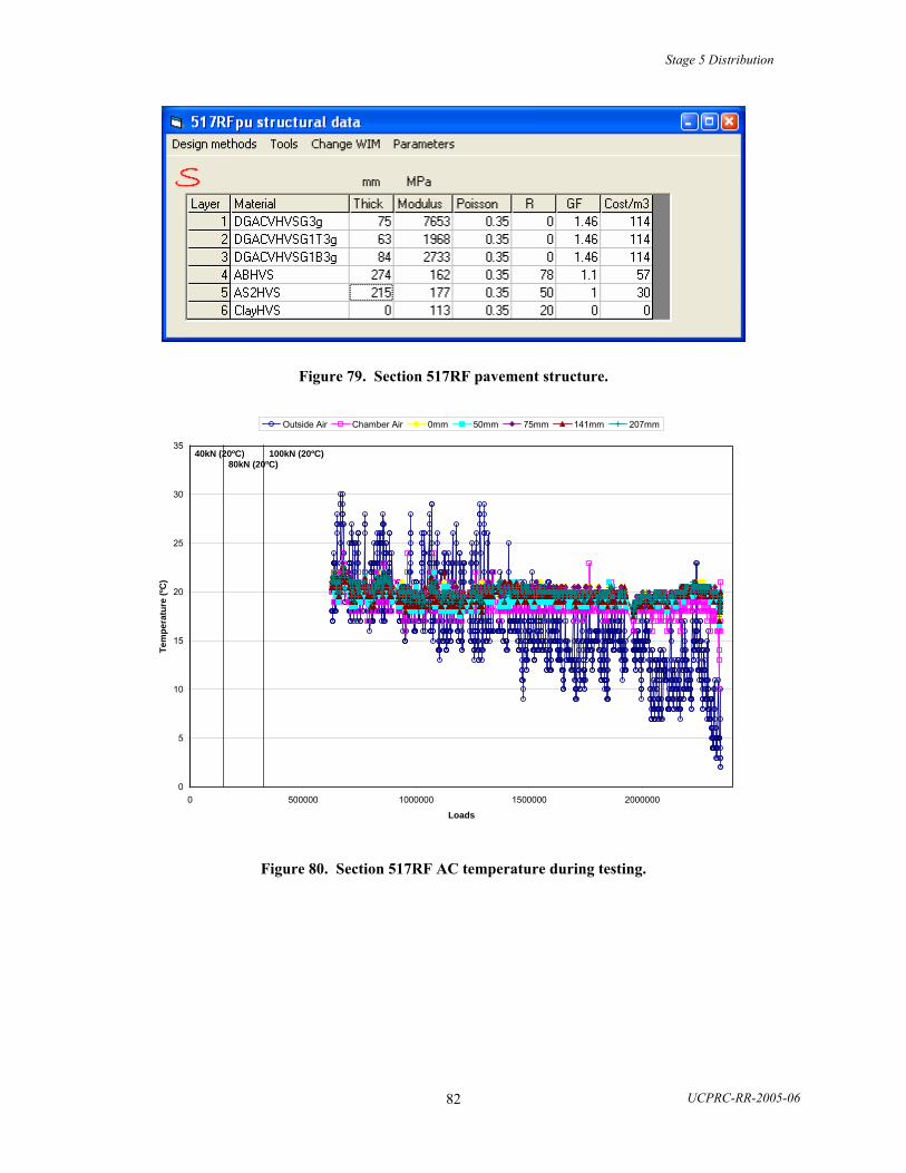
Stage 5 Distribution
UCPRC-RR-2005-06 82
Figure 79. Section 517RF pavement structure.
0
5
10
15
20
25
30
35
0 500000 1000000 1500000 2000000
Loads
Tem
pera
ture
(ºC
)
Outside Air Chamber Air 0mm 50mm 75mm 141mm 207mm
40kN (20ºC) 80kN (20ºC)
100kN (20ºC)
Figure 80. Section 517RF AC temperature during testing.

Stage 5 Distribution
UCPRC-RR-2005-06 83
Figure 81. Section 517RF 40 kN deflection of top modules.
Figure 82. Section 517RF 40 kN compression of pavement layers.

Stage 5 Distribution
UCPRC-RR-2005-06 84
Figure 83. Section 517RF deflection of subgrade.
Figure 84. Section 517RF 100 kN top modules deflection.

Stage 5 Distribution
UCPRC-RR-2005-06 85
Figure 85. Section 517RF 100 kN compression of pavement layers.
Figure 86. Section 517RF 100 kN deflection of subgrade.
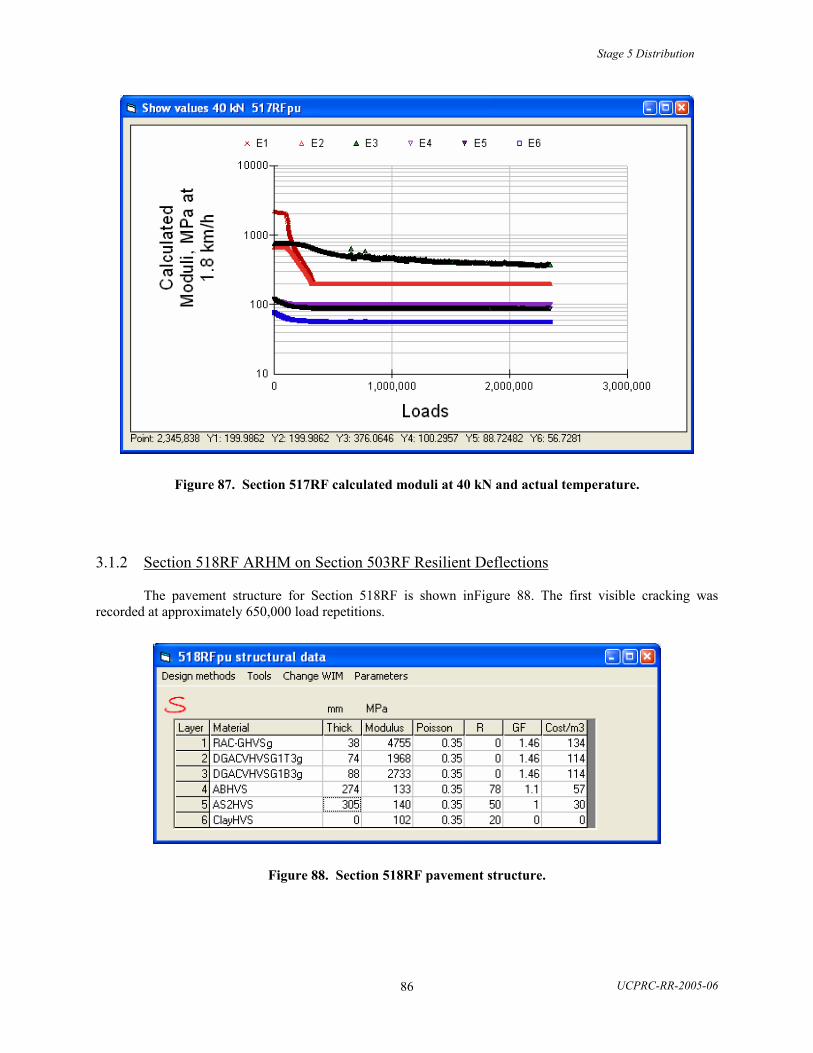
Stage 5 Distribution
UCPRC-RR-2005-06 86
Figure 87. Section 517RF calculated moduli at 40 kN and actual temperature.
3.1.2 Section 518RF ARHM on Section 503RF Resilient Deflections
The pavement structure for Section 518RF is shown inFigure 88. The first visible cracking was recorded at approximately 650,000 load repetitions.
Figure 88. Section 518RF pavement structure.

Stage 5 Distribution
UCPRC-RR-2005-06 87
0
5
10
15
20
25
30
35
0 200000 400000 600000 800000 1000000 1200000 1400000 1600000 1800000
Loads
Tem
pera
ture
(ºC
)
Outside Air Chamber Air 0mm 36mm 50mm 75mm 141mm 217mm
40kN (20ºC) 80kN (20ºC)
100kN (20ºC)
Figure 89. Section 518RF AC temperature during testing.
Figure 90. Section 518RF 40 kN top modules deflection.

Stage 5 Distribution
UCPRC-RR-2005-06 88
Figure 91. Section 518RF 40 kN resilient compression of pavement layers.
Figure 92. Section 518RF 40 kN deflection of subgrade.

Stage 5 Distribution
UCPRC-RR-2005-06 89
Figure 93. Section 518RF 100 kN top modules deflection.
Figure 94. Section 518RF 100 kN compression of pavement layers.

Stage 5 Distribution
UCPRC-RR-2005-06 90
Figure 95. Section 518RF 100 kN deflection of subgrade.
Figure 96. Section 518RF calculated moduli at 40 kN and actual temperature.

Stage 5 Distribution
UCPRC-RR-2005-06 91
3.1.3 Section 514RF DGAC on Section 500RF Resilient Deflections
The pavement structure for Section 514RF is shown in Figure 97. The first visible cracking was recorded at approximately 800,000 load repetitions.
Figure 97. Section 514RF pavement structure.
0
5
10
15
20
25
30
35
40
0 200000 400000 600000 800000 1000000 1200000 1400000 1600000 1800000
Loads
Tem
pera
ture
(ºC
)
Outside Air Chamber Air 0mm 50mm 134mm 200mm 270mm
40kN (20ºC) 80kN (20ºC)
100kN (20ºC)
Figure 98. Section 514RF AC temperature during testing.

Stage 5 Distribution
UCPRC-RR-2005-06 92
Figure 99. Section 514RF 40 kN top modules deflection.
Figure 100. Section 514RF 40 kN compression of pavement layers, MDD1 and MDD2.

Stage 5 Distribution
UCPRC-RR-2005-06 93
Figure 101. Section 514RF 40 kN compression of pavement layers, MDD3 and MDD4.
Figure 102. Section 514RF 40 kN deflection of subgrade.

Stage 5 Distribution
UCPRC-RR-2005-06 94
Figure 103. Section 514RF 100 kN top modules deflection.
Figure 104. Section 514RF 100 kN compression of pavement layers, MDD1 and MDD2.

Stage 5 Distribution
UCPRC-RR-2005-06 95
Figure 105. Section 514RF 100 kN compression of pavement layers, MDD3 and MDD4.
Figure 106. Section 514RF 100 kN deflection of subgrade.

Stage 5 Distribution
UCPRC-RR-2005-06 96
Figure 107. Section 514RF calculated moduli at 40 kN and actual temperature.
3.1.4 Section 515RF ARHM on Section 502CT Resilient Deflections
The pavement structure for Section 515RF is shown in Figure 108. The first visible cracking was recorded at approximately 510,000 load repetitions.
Figure 108. Section 515RF pavement structure.

Stage 5 Distribution
UCPRC-RR-2005-06 97
0
5
10
15
20
25
30
35
40
0 500000 1000000 1500000 2000000
Loads
Tem
pera
ture
(ºC
)
Outside Air Chamber Air 0mm 50mm 108mm 193mm 270mm
40kN (20ºC) 80kN (20ºC)
100kN (20ºC)
Figure 109. Section 515RF AC temperature during testing.
Figure 110. Section 515RF 40 kN top modules deflection.

Stage 5 Distribution
UCPRC-RR-2005-06 98
Figure 111. Section 515RF 40 kN resilient compression of pavement layers.
Figure 112. Section 515RF 40 kN deflection of subgrade.

Stage 5 Distribution
UCPRC-RR-2005-06 99
Figure 113. Section 515RF 100 kN top modules deflection.
Figure 114. Section 515RF 100 kN compression of pavement layers.

Stage 5 Distribution
UCPRC-RR-2005-06 100
Figure 115. Section 515RF 100 kN deflection of subgrade.
Figure 116. Section 515RF calculated moduli at 40 kN and actual temperatures.

Stage 5 Distribution
UCPRC-RR-2005-06 101
3.2 Visual Cracking Versus Damage of the Overlay, Goal 3, 20ºC
Figure 117 shows the visual cracking, in m/m2, as a function of the relative decrease in the overlay modulus. The first appearance of surface cracking occurs at a decrease in modulus similar to that observed for the original structures of Goal 1 (shown in Figure 61) but the growth in visual cracking with decrease in modulus is much faster than for the original structures.
There is no clear difference between the DGAC and the ARHM, or between the drained and the undrained sections.
Visual cracking versus decrease in modulus
0
1
2
3
4
5
6
7
8
9
0 0.2 0.4 0.6 0.8 1
dE/Ei
Cra
ckin
g, m
/m2
517RF DGAC518RF ARHM514RF DGAC515RF ARHM
Figure 117. Cracking in overlay versus relative decrease in modulus of overlay, Goal 3.
There is very little increase in deflection with an increase in the amount of cracking observed at the surface, as can be seen in Figure 118. In some cases the deflection actually decreases with an increase in cracking, indicating that the increase in visual cracking is not directly related to a decrease in modulus. This confirms the tendency shown in Figure 117. This suggests that most of the damage, and the increase in deflections, has occurred prior to the appearance of visible cracks on the surface.

Stage 5 Distribution
UCPRC-RR-2005-06 102
Cracking versus relative deflection
0
1
2
3
4
5
6
7
8
1 1.5 2 2.5 3
Deflection/initial deflection
Cra
ckin
g m
/m2
517RF DGAC518RF ARHM514RF DGAC515RF ARHM
Figure 118. Goal 3, 20ºC, cracking versus increase in deflection.
Table 20 shows the calculated layer moduli at a wheel speed of 1.8 km/h, a load of 40 kN, and the actual temperatures at the start of the test, and Table 21 shows the calculated moduli at the end of the test. Moduli are given in MPa.

Stage 5 Distribution
UCPRC-RR-2005-06 103
Table 20. Layered Moduli at Start of Test, MPa
Start Section517RF
Section 518RF
Section 514RF
Section 515RF
(Original section) (501RF) (503RF) (500RF) (502CT)
Overlay type DGAC ARHM DGAC ARHM
Overlay 2204 1649 2313 1722
AC top 671 755 912 1078
AC bottom 762 950 1187 1645
ATPB 411 444
AB 118 111 143 128
ASB 119 110 135 118
Subgrade 77 78 78 129
Table 21. Layer Moduli at End of Test, MPa
Final Section 517RF
Section 518RF
Section 514RF
Section 515RF
Overlay type
DGAC ARHM DGAC ARHM
Overlay 427 329 727 442
AC top 200 200 200 200
AC bottom 439 329 589 343
ATPB 200 200
AB 101 100 105 102
ASB 90 88 93 88
Subgrade 58 59 56 95
The percentage decrease in moduli is given in Table 22. The trends are similar to those of the Goal 1 fatigue cracking.

Stage 5 Distribution
UCPRC-RR-2005-06 104
Table 22. Percentage Decrease in Moduli
% Decrease Section 517RF
Section 518RF
Section 514RF
Section 515RF
Overlay type DGAC ARHM DGAC ARHM
Overlay 81 80 69 74
AC top 70 74 78 81
AC bottom 42 65 50 79
ATPB 51 55
AB 14 10 27 20
ASB 24 20 31 25
Subgrade 25 24 28 26
3.3 Permanent Deformation Goal 3, 20ºC
The permanent deformations, accumulated during the Goal 1 testing, were assumed to remain as initial permanent deformations in Goal 3, and it is assumed that there was no recovery of permanent deformation from Goal 1 to Goal 3. The deformations are given (in mm) in Table 23.
Table 23. Initial Permanent Deformations, Goal 3, in mm
Section (517RF) (518RF) (514RF) (515RF)
Overlay type
DGAC ARHM DGAC ARHM
(Original) Test
Section
501RF 503RF 500RF 502CT
AC top 3.6 3.4 4.0 3.2
AC bottom 0.0 0.0 0.0 0.0
ATPB 0.0 0.0
AB 2.7 3.3 3.5 3.2
ASB 1.0 1.2 1.8 1.6
Subgrade 1.4 1.2 3.2 1.7

Stage 5 Distribution
UCPRC-RR-2005-06 105
3.3.1 Section 517RF 75-mm DGAC Permanent Deformations
Figure 119. Section 517RF permanent deformation of AC layers.
Figure 120. Section 517RF permanent deformation of granular layers.

Stage 5 Distribution
UCPRC-RR-2005-06 106
Figure 121. Section 517RF permanent deformation of subgrade.
517RF DGAC
-10
-9
-8
-7
-6
-5
-4
-3
-2
-1
0
0 500000 1000000 1500000 2000000 2500000Number of load repetitions
Perm
anen
t def
orm
atio
n, m
m
MDD9-0mmProfile AvgCalculated
Figure 122. Section 517RF permanent deformation at pavement surface.

Stage 5 Distribution
UCPRC-RR-2005-06 107
3.3.2 Section 518RF 38-mm ARHM Permanent Deformation
Figure 123. Section 518RF permanent deformation of AC layers.
Figure 124. Section 518RF permanent deformation of granular layers.

Stage 5 Distribution
UCPRC-RR-2005-06 108
Figure 125. Section 518RF permanent deformation of subgrade.
518RF ARHM
-5
-4
-3
-2
-1
0
0 500000 1000000 1500000 2000000Number of load repetitions
Perm
anen
t def
orm
atio
n, m
m
MDD10-0mmProfile AvgCalculated
Figure 126. Section 518RF permanent deformation at pavement surface.

Stage 5 Distribution
UCPRC-RR-2005-06 109
3.3.3 Section 514RF 75-mm DGAC Permanent Deformations
Figure 127. Section 514RF permanent deformation of AC layers.
Figure 128. Section 514RF permanent deformation of granular layers, MDD1 and MDD2.

Stage 5 Distribution
UCPRC-RR-2005-06 110
Figure 129. Section 514RF permanent deformation of granular layers, MDD3 and MDD4.
Figure 130. Section 514RF permanent deformation of subgrade.

Stage 5 Distribution
UCPRC-RR-2005-06 111
514RF DGAC
-9
-8
-7
-6
-5
-4
-3
-2
-1
0
0 500000 1000000 1500000 2000000Number of load repetitions
Perm
anen
t def
orm
atio
n, m
mMDD10-0mmProfile AvgCalculated
Figure 131. Section 514RF permanent deformation at pavement surface.

Stage 5 Distribution
UCPRC-RR-2005-06 112
3.3.4 Section 515RF 38-mm ARHM Permanent Deformations
Figure 132. Section 515RF permanent deformation of AC layers.
Figure 133. Section 515RF permanent deformation of granular layers.

Stage 5 Distribution
UCPRC-RR-2005-06 113
Figure 134. Section 515RF permanent deformation of subgrade.
515RF ARHM
-6
-5
-4
-3
-2
-1
0
0 500000 1000000 1500000 2000000 2500000Number of load repetitions
Perm
anen
t def
orm
atio
n, m
m
MDD10-0mmProfile AvgCalculated
Figure 135. Section 515RF permanent deformation of the pavement surface.

Stage 5 Distribution
UCPRC-RR-2005-06 114
4.0 GOAL 3 RUTTING EXPERIMENTS
The HVS Goal 3 rutting tests were performed on overlays placed on Goal 1 pavements that had not been previously loaded. The overlays were the same materials as in the Goal 3, 20ºC experiments, but of varying thicknesses for the ARHM.
Several different wheels were used in these tests. The tire pressures are given in Table 24. Table 24. Tire Types and Pressure, MPa
Tire-type MPa
Bias-ply duals 0.620
Radial duals 0.723
Wide-Base single 0.758
Aircraft 1.034
All loading was unidirectional with a wheel load of 40 kN, except for Section 513RF. Loading on that section was done bidirectionally with the aircraft tire and a wheel load of 100 kN. Testing was done at elevated temperatures of 45–50ºC.
Unidirectional loading has been found to result in larger rut depth than bidirectional loading. In Florida Tia et al. (28) found from HVS tests reported in 2002 that:
Athough the bi-directional mode can apply almost twice the number of wheel passes per day as compared with the unidirectional mode, the unidirectional mode of loading still produced slightly higher rut depths for the same testing duration.
To compensate for this difference the value of K (the ratio between rut depth and permanent shear strain) was multiplied by a factor of 1.6 to give 0.13 for Goal 1 materials and 0.4 for all other materials.
The test sections were not instrumented with MDDs, but their surface profile was measured. No cracking was observed, but the same fatigue models used in the 20ºC testing were used here too. They resulted in a considerable amount of predicted damage. The validity of the fatigue models at elevated temperatures is not known.

Stage 5 Distribution
UCPRC-RR-2005-06 115
4.1 Section 504RF No Overlay, Wide-Base Single Tire
Temperature data was not available. A temperature profile with 48.5ºC at the top and 35ºC at a depth of 150 mm was estimated from data in Harvey et al. (2002), and used during the entire test.
Figure 136. Section 504RF pavement structure.
Figure 137. Section 504RF permanent deformation at pavement surface from profilometer.

Stage 5 Distribution
UCPRC-RR-2005-06 116
Figure 138. Section 504RF calculated permanent deformation of pavement layers.
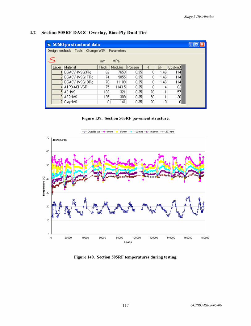
Stage 5 Distribution
UCPRC-RR-2005-06 117
4.2 Section 505RF DAGC Overlay, Bias-Ply Dual Tire
Figure 139. Section 505RF pavement structure.
0
10
20
30
40
50
60
70
0 20000 40000 60000 80000 100000 120000 140000 160000 180000
Loads
Tem
pera
ture
(ºC
)
Outside Air 0mm 50mm 100mm 165mm 237mm
40kN (50ºC)
Figure 140. Section 505RF temperatures during testing.

Stage 5 Distribution
UCPRC-RR-2005-06 118
Figure 141. Section 505RF permanent deformation at pavement surface from profilometer.
Figure 142. Section 505RF calculated permanent deformation of pavement layers.

Stage 5 Distribution
UCPRC-RR-2005-06 119
4.3 Section 506RF DGAC Overlay, Radial Dual Tire
Figure 143. Section 506RF pavement structure.
0
10
20
30
40
50
60
0 20000 40000 60000 80000 100000 120000 140000 160000 180000
Loads
Tem
pera
ture
(ºC
)
Outside Air 0mm 50mm 76mm 138mm 214mm
40kN (50ºC)
Figure 144. Section 506RF temperatures during testing.

Stage 5 Distribution
UCPRC-RR-2005-06 120
Figure 145. Section 506RF permanent deformation at pavement surface from profilometer.
Figure 146. Section 506RF calculated permanent deformation of pavement layers.

Stage 5 Distribution
UCPRC-RR-2005-06 121
4.4 Section 507RF DGAC Overlay, Wide-Base Single Tire
Figure 147. Section 507RF pavement structure.
0
10
20
30
40
50
60
70
0 20000 40000 60000 80000 100000
Loads
Tem
pera
ture
(ºC
)
Outside Air 0mm 50mm 76mm 138mm 214mm
40kN (50ºC)
Figure 148. Section 507RF temperatures during testing.

Stage 5 Distribution
UCPRC-RR-2005-06 122
Figure 149. Section 507RF permanent deformation at pavement surface from profilometer.
Figure 150. Section 507RF calculated permanent deformation of pavement layers.

Stage 5 Distribution
UCPRC-RR-2005-06 123
4.5 Section 508RF ARHM Overlay, Wide-Base Single Tire
Figure 151. Section 508RF pavement structure.
0
10
20
30
40
50
60
70
0 20000 40000 60000 80000 100000 120000
Loads
Tem
pera
ture
(ºC
)
Outside Air 0mm 50mm 61mm 137mm 213mm
40kN (50ºC)
Figure 152. Section 508RF temperatures during testing.

Stage 5 Distribution
UCPRC-RR-2005-06 124
Figure 153. Section 508RF permanent deformation at pavement surface from profilometer.
Figure 154. Section 508RF calculated permanent deformation of pavement layers.

Stage 5 Distribution
UCPRC-RR-2005-06 125
4.6 Section 509RF ARHM Overlay, Radial Dual Tire
Figure 155. Section 509RF pavement structure.
0
10
20
30
40
50
60
70
0 20000 40000 60000 80000 100000 120000 140000 160000 180000 200000
Loads
Tem
pera
ture
(ºC
)
Outside Air 0mm 50mm 61mm 137mm 213mm
40kN (50ºC)
Figure 156. Section 509RF temperatures during testing.

Stage 5 Distribution
UCPRC-RR-2005-06 126
Figure 157. Section 509RF permanent deformation at pavement surface from profilometer.
Figure 158. Section 509RF calculated permanent deformation of pavement layers.

Stage 5 Distribution
UCPRC-RR-2005-06 127
4.7 Section 510RF ARHM Overlay, Radial Dual Tire
Figure 159. Section 510RF pavement structure.
0
10
20
30
40
50
60
70
0 20000 40000 60000 80000 100000 120000 140000 160000 180000 200000
Loads
Tem
pera
ture
(ºC
)
Outside Air 0mm 37mm 50mm 112mm 187mm
40kN (50ºC)
Figure 160. Section 510RF temperatures during testing.

Stage 5 Distribution
UCPRC-RR-2005-06 128
Figure 161. Section 510RF permanent deformation at pavement surface from profilometer.
Figure 162. Section 510RF calculated permanent deformation of pavement layers.

Stage 5 Distribution
UCPRC-RR-2005-06 129
4.8 Section 511RF ARHM Overlay, Wide-Base Single Tire
Figure 163. Section 511RF pavement structure.
0
10
20
30
40
50
60
0 10000 20000 30000 40000 50000 60000 70000 80000
Loads
Tem
pera
ture
(ºC
)
Outside Air 0mm 37mm 50mm 112mm 187mm
40kN (50ºC)
Figure 164. Section 511RF temperatures during testing.

Stage 5 Distribution
UCPRC-RR-2005-06 130
Figure 165. Section 511RF permanent deformation at the pavement surface.
Figure 166. Section 511RF calculated permanent deformation of the pavement layers.

Stage 5 Distribution
UCPRC-RR-2005-06 131
4.9 Section 512RF DGAC Overlay, Wide-Base Single Tire
Figure 167. Section 512RF pavement structure.
0
10
20
30
40
50
60
0 50000 100000 150000 200000 250000 300000 350000
Loads
Tem
pera
ture
(ºC
)
Outside Air 0mm 37mm 50mm 112mm 187mm
40kN (40ºC)
Figure 168. Section 512RF temperatures during testing.

Stage 5 Distribution
UCPRC-RR-2005-06 132
Figure 169. Section 512RF permanent deformation at pavement surface from profilometer.
Figure 170. Section 512RF calculated permanent deformation of the pavement layers.

Stage 5 Distribution
UCPRC-RR-2005-06 133
4.10 Section 513RF DGAC Overlay, Aircraft Tire
Figure 171. Section 513RF pavement structure.
Temperature data was not available in the database. The following temperatures were estimated from data in Harvey et al. (2000).
Table 25. Estimated Temperatures for Section 513RF
Depth, mm 0 25 50 75 100 125 150 175 200 225
Temperature, ºC 51 49.5 48 44.5 43 41.5 40 39 37.5 37

Stage 5 Distribution
UCPRC-RR-2005-06 134
Figure 172. Section 513RF permanent deformation at pavement surface from profilometer.
Figure 173. Section 513RF calculated permanent deformation of pavement layers.

Stage 5 Distribution
UCPRC-RR-2005-06 135
5.0 GOAL 5 WET CONDITIONS
As Section 1 notes, in each of the Goal 5 tests water from a drip system was introduced into the HVS test section pavements. The water entered the pavements at the top of their base layers (either ATPB or aggregate) through holes drilled on the sections’ upstream side.
In the simulations a slip was assumed to develop between the two AC layers of Goal 1 (as in the simulations of Goal 1 and Goal 3). There was clear evidence that slip also developed between the overlay and the AC top layer of Goal 1 at some locations, and that the ATPB of Section 543RF disintegrated (as shown Figure 174).
Figure 174. Cores from trafficked area of Section 543RF after HVS loading show stripping and disintegration of ATPB, as well as signs of moisture damage between the the three lifts of asphalt
concrete (Bejarano et al. 2003).
To get reasonably good agreement between calculated and measured deflections, the stiffness factorsof the unbound materials, previously discussed in Section 1.5.2 of this report (see Equations 17 and 18) were assumed to be 0.55, 0.45, and 0.3 for AB, ASB, and subgrade, respectively. These are the same values used during Goal 1 and Goal 3 for simulations with full bond. It would have been more consistent for the research team to use the same stiffness factor values that it did when simulating slip conditions in Goal 1 and Goal 3 (although the wet conditions could have resulted in different values than the dry condition). However, several attempts to combine those values with different slips at different interfaces failed to produce reasonably good agreement between the measured and calculated responses. This could be due to the difficulty of simulating the correct slip conditions. The above values were used instead because of the importance of having the correct response for calibrating fatigue and permanent deformation parameters.

Stage 5 Distribution
UCPRC-RR-2005-06 136
Only a few Multi-depth Deflectometer (MDD) modules functioned correctly during the wet testing. The moduli of the unbound layers were chosen to give a reasonably good agreement with the initial deflections measured with these MDDs and with the Road Surface Deflectometer (RSD). For the asphalt layers the same moduli were used as in the previous simulations, i.e., from frequency sweep data. The asphalt fatigue models and the permanent deformation models were also the same as in the previous simulations.
5.1 Section 543RF ARHM Overlay, Drained
Figure 175 shows the pavement structure for Section 543RF. It was assumed that a slip developed between layer 2 and layer 3 at 8 million ESALs (corresponding to approximately 600,000 load repetitions using the Caltrans 4.2 exponent). The models did not do well calculating the permanent deformation of the ATPB and the granular base after the stripping and collapse of the ATPB at about 600,000 repetitions. The modeled pavement appears to have simulated response and performance prior to the collapse fairly well.
Figure 175. Section 543RF pavement structure.

Stage 5 Distribution
UCPRC-RR-2005-06 137
0
5
10
15
20
25
30
0 200000 400000 600000 800000 1000000 1200000
Loads
Tem
pera
ture
(ºC
)
Outside Air Chamber Air 0mm 38mm 104mm 170mm 245mm
40kN (20ºC) 80kN (20ºC) 100kN (20ºC)
Figure 176. Section 543RF temperatures during testing.
Figure 177. Section 543RF Road Surface Deflectometer, at 40 kN.

Stage 5 Distribution
UCPRC-RR-2005-06 138
Figure 178. Section 543RF Road Surface Deflectometer, at 100 kN.
Figure 179. Section 543RF 40 kN top module.

Stage 5 Distribution
UCPRC-RR-2005-06 139
Figure 180. Section 543RF 40 kN top of aggregate base.
Figure 181. Section 543RF 40 kN top of aggregate subbase.

Stage 5 Distribution
UCPRC-RR-2005-06 140
Figure 182. Section 543RF 40 kN deflection of subgrade (850 mm depth).
Figure 183. Section 543RF 100 kN top module.

Stage 5 Distribution
UCPRC-RR-2005-06 141
Figure 184. Section 543RF 100 kN top of aggregate base.
Figure 185. Section 543RF 100 kN top of aggregate subbase.

Stage 5 Distribution
UCPRC-RR-2005-06 142
Figure 186. Section 543RF 100 kN deflection of subgrade (850 mm depth).
Figure 187. Section 543RF Permanent deformation of asphalt layers.

Stage 5 Distribution
UCPRC-RR-2005-06 143
Figure 188. Section 543RF permanent deformation of granular layers plus top of subgrade.
Figure 189. Section 543RF permanent deformation in subgrade (850 mm depth).

Stage 5 Distribution
UCPRC-RR-2005-06 144
543RF ARHM overlay, drained
-25
-20
-15
-10
-5
0
0 500000 1000000 1500000Number of load repetitions
Perm
anen
t def
orm
atio
n, m
mMDD7-0mmProfile AvgCalculated
Figure 190. Section 543RF permanent deformation at pavement surface.
Figure 191. Section 543RF calculated layer moduli, at 40 kN and actual temperatures.

Stage 5 Distribution
UCPRC-RR-2005-06 145
5.2 Section 544RF ARHM Overlay, Undrained
The pavement structure for Section 544RF is shown in Figure 192. Slip was assumed to develop between layer 2 and layer 3 at 2 million ESALs (corresponding to approximately 300,000 load repetitions).
Figure 192. Section 544RF pavement structure.
0
5
10
15
20
25
30
35
0 200000 400000 600000 800000 1000000 1200000
Loads
Tem
pera
ture
(ºC
)
Outside Air Chamber Air 0mm 38mm 104mm 170mm 245mm
40kN (20ºC) 80kN (20ºC) 100kN (20ºC)
Figure 193. Section 544RF temperatures during testing.

Stage 5 Distribution
UCPRC-RR-2005-06 146
Figure 194. Section 544RF Road Surface Deflectometer, at 40 kN.
Figure 195. Section 544RF Road Surface Deflectometer, at 100 kN.

Stage 5 Distribution
UCPRC-RR-2005-06 147
Figure 196. Section 544RF 40 kN top module.
Figure 197. Section 544RF 40 kN top of aggregate base.

Stage 5 Distribution
UCPRC-RR-2005-06 148
Figure 198. Section 544RF 40 kN top of aggregate subbase.
Figure 199. Section 544RF 100 kN top module.

Stage 5 Distribution
UCPRC-RR-2005-06 149
Figure 200. Section 544RF 100 kN top of aggregate base.
Figure 201. Section 544RF 100 kN top of aggregate subbase.
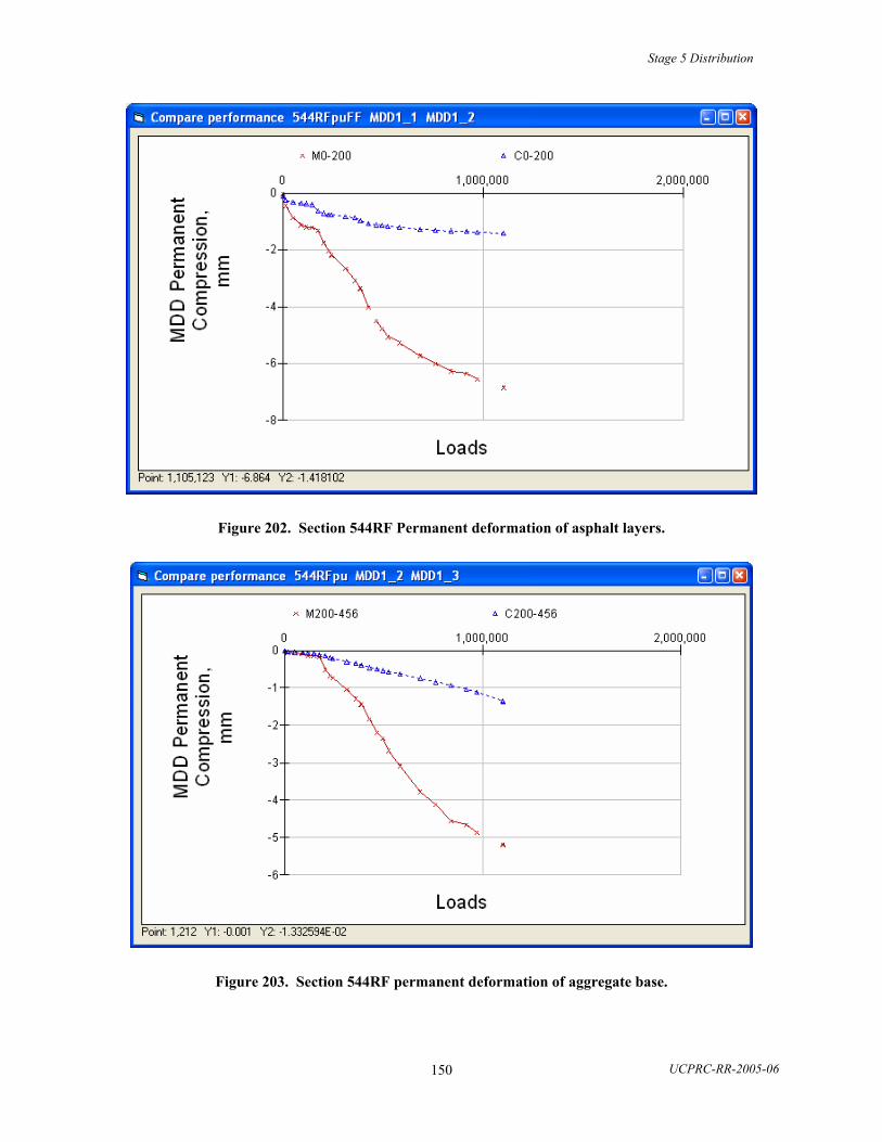
Stage 5 Distribution
UCPRC-RR-2005-06 150
Figure 202. Section 544RF Permanent deformation of asphalt layers.
Figure 203. Section 544RF permanent deformation of aggregate base.

Stage 5 Distribution
UCPRC-RR-2005-06 151
Figure 204. Section 544RF permanent deformation on top of basecourse.
544RF ARHM overlay, undrained
-16
-14
-12
-10
-8
-6
-4
-2
0
0 500000 1000000 1500000Number of load repetitions
Perm
anen
t def
orm
atio
n, m
m
MDD7-0mmProfile AvgCalculated
Figure 205. Section 544RF permanent deformation at pavement surface.

Stage 5 Distribution
UCPRC-RR-2005-06 152
Figure 206. Section 544RF calculated moduli of pavement layers.

Stage 5 Distribution
UCPRC-RR-2005-06 153
5.3 Section 545RF DGAC Overlay, Undrained
The pavement structure for Section 545RF is shown in Figure 207. Slip between layer 2 and layer 3 was assumed to develop at 200,000 ESALs (corresponding to approximately 200,000 load repetitions).
Figure 207. Section 545RF pavement structure.
0
5
10
15
20
25
30
35
0 100000 200000 300000 400000 500000 600000 700000 800000
Loads
Tem
pera
ture
(ºC
)
Outside Air 0mm 50mm 75mm 108mm 174mm 235mm
40kN (20ºC) 80kN (20ºC) 100kN (20ºC)
Figure 208. Section 545RF temperatures during testing.

Stage 5 Distribution
UCPRC-RR-2005-06 154
Figure 209. Section 545RF Road Surface Deflectometer, at 40 kN.
Figure 210. Section 545RF Road Surface Deflectometer, 100 kN.

Stage 5 Distribution
UCPRC-RR-2005-06 155
Figure 211. Section 545RF 40 kN top module.
Figure 212. Section 545RF 40 kN top of aggregate base.

Stage 5 Distribution
UCPRC-RR-2005-06 156
Figure 213. Section 545RF 40 kN top of aggregate subbase.
Figure 214. Section 545RF 100 kN top module.

Stage 5 Distribution
UCPRC-RR-2005-06 157
Figure 215. Section 545RF 100 kN top of aggregate base.
Figure 216. Section 545RF 100 kN top of aggregate subbase.

Stage 5 Distribution
UCPRC-RR-2005-06 158
Figure 217. Section 545RF permanent deformation of asphalt layers.
Figure 218. Section 545RF permanent deformation of aggregate base.

Stage 5 Distribution
UCPRC-RR-2005-06 159
545RF DGAC overlay, undrained
-8
-7
-6
-5
-4
-3
-2
-1
0
0 500000 1000000Number of load repetitions
Perm
anen
t def
orm
atio
n, m
mMDD8-0mmProfile AvgCalculated
Figure 219. Section 545RF permanent deformation at pavement surface.
Figure 220. Section 545RF calculated moduli of pavement layers.

Stage 5 Distribution
UCPRC-RR-2005-06 160
5.4 Visual Cracking versus Damage of the Top Asphalt Layer, Goal 5
Figure 221 shows visual cracking (in m/m2) versus the relative decrease in the modulus of the overlay. As was the case for the previous simulations, visual cracking was not observed before the calculated modulus of the overlay had dropped by 50–60 percent. The difference between drained and undrained sections is similar to the difference in Goal 1, with the drained sections showing cracking at a greater loss of stiffness than the undrained sections.
Goal 5 Wet conditions
0
1
2
3
4
5
6
7
0 0.2 0.4 0.6 0.8 1
dE/Ei
Cra
ckin
g, m
/m2
543RF ARHM drained544RF ARHM undrained545RF DGAC undrained
Figure 221. Visual cracking versus relative decrease in modulus of layer 1, Goal 5 Wet conditions.

Stage 5 Distribution
UCPRC-RR-2005-06 161
Cracking versus relative deflection
0
1
2
3
4
5
6
7
1 1.5 2 2.5 3 3.5 4 4.5
Deflection/initial deflection
Cra
ckin
g m
/m2
543RF ARHM drained544RF ARHM undrained545RF DGAC undrained
Figure 222. Goal 5, cracking versus increase in deflection.

Stage 5 Distribution
UCPRC-RR-2005-06 162
6.0 GOAL 9 MODIFIED BINDER (MB) ROAD, INITIAL TESTS
6.1 Materials Characterization
Modulus parameters for the Goal 9 asphalt concrete (AC) are shown in Figure 223. It should be noted that the binder for the asphalt concrete in these sections is conventional and unmodified. Modified binders (MB) were used for the subsequent overlays, for which testing is still underway, and they are not considered in this report.
Figure 223. MB road, AC modulus-versus-reduced time parameters from frequency sweep.
The modulus-versus-reduced time parameters were determined from frequency sweep testing and are shown in Figure 223. These were the parameters used in the CalME simulations.
FWD testing was carried out at different intervals during the HVS experiments. The moduli of the layers were determined from backcalculation using Elmod5 software. The tests were done at the center line of the road from September 2001 to May 2003. The asphalt layer moduli are influenced by both temperature and aging effects.

Stage 5 Distribution
UCPRC-RR-2005-06 163
Modulus of asphalt, Goal 9
100
1000
10000
100000
0 10 20 30 40 50
Temperature, C
Mod
ulus
, MPa
FWDFrequency sweepFitted FWD
Figure 224. Moduli from FWD compared to frequency sweep tests, Goal 9 (MB road).
Although there is a large scatter in the backcalculated moduli (as seen in Figure 224), the values appear to be considerably lower than those from frequency sweep tests, at intermediate temperatures. It should be noted that the thickness of the asphalt layer is close to the lower limit for backcalculation of the modulus. However, the tendency is the same as for Goal 1 (where it could have been influenced by slip between the two asphalt layers). The parameters for the best fit to the FWD data are shown in Table 26.
Another possible explanation for the difference in moduli is a difference in strain level. Laboratory tests have shown that greater strain levels result in lower stiffnesses. At 20°C and a frequency of 5 Hz, shear frequency sweep data showed a decrease in shear stiffness from 668 to 1666 to 1918 MPa for shear strains of 1000, 500, and 100 μstrain, respectively (Harvey, Guada, and Long, AAPT 2000). The FWD has greater strain (about 300 μstrain) than the flexural frequency sweep tests (about 200 μstrain), which helps explain the difference.

Stage 5 Distribution
UCPRC-RR-2005-06 164
Table 26. Parameters for FWD Moduli versus Reduced Time, Goal 9
Reference Modulus 3333 MPa
Reference Temperature 20ºC
δ 2.6021
β 1.1266
γ 0.8059
α 1.5740
aT 1.3370
A 9.6307
VTS -3.5047
Damage parameters for the AC were determined from laboratory beam controlled-strain fatigue testing. The parameters are shown in the first column of Figure 225. A shift factor of 3 was used, as for the previous simulations.
The same parameters used for the conventional Goal 3 simulations were used (column 2 of Figure 225) for permanent deformation of the AC layer.
The aggregate base (AB) was 100 percent recycled material with a high content of recycled portland cement concrete. Figure 226 shows the backcalculated moduli plotted against time. The moduli are average values for the full test line using drop 2, corresponding to a load level of approximately 40 kN. The first six points were determined during autumn of 2001 and early winter of 2002, and the last two tests were done after the summer of 2002. Some of the moduli variation may be due to changes in the temperature of the AC layer but some must be due to self-cementing of the PCC in the AB layer. A purely granular material, without any cohesion, cannot achieve layer moduli of 800–1200 MPa.

Stage 5 Distribution
UCPRC-RR-2005-06 165
Figure 225. MB road, damage parameters for AC in first column.

Stage 5 Distribution
UCPRC-RR-2005-06 166
MB road, AB modulus
0.0
200.0
400.0
600.0
800.0
1000.0
1200.0
1400.0
9/1/2001 4/1/2002 10/31/2002 5/31/2003
Date
Mod
ulus
, MPa
Figure 226. MB road, backcalculated modulus of AB versus time.
MB road, modulus of AB
y = 146.89x + 238.8R2 = 0.699
y = 265.26x + 641.11R2 = 1
0.0
200.0
400.0
600.0
800.0
1000.0
1200.0
1400.0
0.0000 0.5000 1.0000 1.5000 2.0000 2.5000
Stiffness ratio
Mod
ulus
, MPa
2001-20022003Linear (2001-2002)Linear (2003)
Figure 227. MB road, modulus of AB versus stiffness of AC.

Stage 5 Distribution
UCPRC-RR-2005-06 167
In Figure 227, the modulus of the AB is plotted versus the stiffness ratio calculated as:
3
3
1000ACAC Eh
ratioStiffness×
= (32)
where hAC is the thickness of the AC (80 mm in the backcalculation), and EAC is the modulus of the AC.
From the two regression lines in Figure 227 the parameters of Equation (18) may be determined:
Table 27. MB Road, Stiffness Parameters for AB
Eo Stiffness Factor
2001-2002 344 0.23
2003 795 0.19
MB road, Subgrade modulus
y = 57.143x + 49.314R2 = 0.9175
0
50
100
150
200
250
300
350
0 1 2 3 4 5
Stiffness ratio
Mod
ulus
, MPa
SubgradeLinear (Subgrade)
Figure 228. MB road, subgrade modulus versus stiffness of pavement layers.
For the subgrade modulus it is not necessary to distinguish between the tests done before and after the summer of 2002. All the test points are plotted in Figure 228 versus the stiffness ratio calculated as:

Stage 5 Distribution
UCPRC-RR-2005-06 168
333
3500 ⎟⎟⎟
⎠
⎞
⎜⎜⎜
⎝
⎛ ×+×=
ABABACAC EhEhratioStiffness (33)
where hAB is the thickness of AB (398 mm in the backcalculation), and EAB is the modulus of the
AB. The regression line for the subgrade in Figure 228 results in:
• Eo = 116 MPa and
• Stiffness factor = 0.46
The stiffness factors given above have been used in the simulations, whereas the moduli of AB and subgrade have been selected to give initial deflections that correspond reasonably well to those measured with the RSD or the MDDs (where available).
When calculating the permanent deformation of AB and subgrade, the same parameters were used as in the previous simulations.
A 61.5 kN dual wheel load was used for all of the testing, except for the part of Section 567RF where a 38.4 kN wheel load was used. The results of the HVS tests are given in chronological order in the following subsection.

Stage 5 Distribution
UCPRC-RR-2005-06 169
6.2 Section 567RF MB Road
The test was carried out from December 21, 2001, to January 20, 2002. The pavement section is shown in Figure 229. Cracking was only recorded at the end of the test, when it had reached 8.2 m/m2.
Figure 229. Section 567RF pavement structure.
Figure 230. Section 567RF load levels.

Stage 5 Distribution
UCPRC-RR-2005-06 170
0
5
10
15
20
25
0 10000 20000 30000 40000 50000 60000 70000 80000
Loads
Tem
pera
ture
(ºC
)
Outside Air Chamber Air 0mm 45mm 90mm
40kN (20ºC) 25kN (20ºC)
Figure 231. Section 567RF temperatures during testing.
Figure 232. Section 567RF Road Surface Deflectometer.

Stage 5 Distribution
UCPRC-RR-2005-06 171
Figure 233. Section 567RF MDDs at 90mm and 330 mm.
Figure 234. Section 567RF permanent deformation of MDDs.

Stage 5 Distribution
UCPRC-RR-2005-06 172
Figure 235. Section 567RF permanent deformation at pavement surface from profilometer.
Figure 236. Section 567RF calculated moduli at 40 kN and actual temperature.

Stage 5 Distribution
UCPRC-RR-2005-06 173
6.3 Section 568RF MB Road
The test was carried out from January 14, 2002, to February 5, 2002. The pavement structure is shown in Figure 237. The first visible cracking was recorded at approximately 198,000 load repetitions.
Figure 237. Section 568RF pavement structure.
0
5
10
15
20
25
0 50000 100000 150000 200000 250000 300000 350000 400000
Loads
Tem
pera
ture
(ºC
)
Outside Air Chamber Air 0mm 45mm 90mm
40kN (20ºC)
Figure 238. Section 568RF temperatures during testing.

Stage 5 Distribution
UCPRC-RR-2005-06 174
Figure 239. Section 568RF Road Surface Deflectometer.
Figure 240. Section 568RF permanent deformation at pavement surface from profilometer.

Stage 5 Distribution
UCPRC-RR-2005-06 175
Figure 241. Section 568RF calculated layer moduli at 40 kN and actual temperature.

Stage 5 Distribution
UCPRC-RR-2005-06 176
6.4 Section 573RF MB Road
The test was carried out from March 20, 2002, to July 8, 2002. The pavement structure is shown in Figure 242. Cracking was only recorded at the end of the test, where it had reached 4.2 m/m2.
Figure 242. Section 573RF pavement structure.
0
5
10
15
20
25
30
35
0 100000 200000 300000 400000 500000 600000 700000 800000 900000 1000000
Loads
Tem
pera
ture
(ºC
)
Outside Air Chamber Air 0mm 45mm 90mm
40kN (20ºC) 30kN (20ºC)
40kN (20ºC)
Figure 243. Section 573RF temperatures during testing.

Stage 5 Distribution
UCPRC-RR-2005-06 177
Figure 244. Section 573RF Road Surface Deflectometer.
Figure 245. Section 573RF permanent deformation at pavement surface from profilometer.

Stage 5 Distribution
UCPRC-RR-2005-06 178
Figure 246. Section 573RF calculated layer moduli at 40 kN and actual temperature.

Stage 5 Distribution
UCPRC-RR-2005-06 179
6.5 Section 571RF MB Road
The test was carried out from July 12, 2002, to October 2, 2002. The pavement structure is shown in Figure 247. The first visible cracking was recorded at approximately 480,000 load repetitions.
Figure 247. Section 571RF pavement structure.
0
5
10
15
20
25
30
35
40
0 100000 200000 300000 400000 500000 600000 700000 800000
Loads
Tem
pera
ture
(ºC
)
Outside Air Chamber Air 0mm 45mm 90mm
40kN (20ºC)
Figure 248. Section 571RF temperatures during testing.

Stage 5 Distribution
UCPRC-RR-2005-06 180
Figure 249. Section 571RF Road Surface Deflectometer.
Figure 250. Section 571RF MDDs at 90 mm, 300 mm, and 525 mm.

Stage 5 Distribution
UCPRC-RR-2005-06 181
Figure 251. Section 571RF permanent deformation of MDDs.
Figure 252. Section 571RF permanent deformation at the pavement surface.

Stage 5 Distribution
UCPRC-RR-2005-06 182
Figure 253. Section 571RF calculated layer moduli at 40 kN and actual temperature.

Stage 5 Distribution
UCPRC-RR-2005-06 183
6.6 Section 572RF MB Road
The test was carried out from January 24, 2003, to March 12, 2003. The pavement structure is shown in Figure 254. The first visible cracking was recorded at approximately 220,000 load repetitions.
Figure 254. Section 572RF pavement structure.
0
5
10
15
20
25
30
0 100000 200000 300000 400000 500000 600000
Loads
Tem
pera
ture
(ºC
)
Outside Air 0mm 50mm 90mm
40kN (20ºC)
Figure 255. Section 572RF temperatures during testing.

Stage 5 Distribution
UCPRC-RR-2005-06 184
Figure 256. Section 572RF Road Surface Deflectometer.
Figure 257. Section 572RF permanent deformation at the pavement surface.

Stage 5 Distribution
UCPRC-RR-2005-06 185
Figure 258. Section 572RF calculated layer moduli at 40 kN and actual temperature.

Stage 5 Distribution
UCPRC-RR-2005-06 186
6.7 Section 569RF MB Road
The test was carried out from March 25, 2003, to April 7, 2003. The pavement structure is shown in Figure 259. Cracking was only recorded at 150,000 load repetitions, where it had reached 5.9 m/m2.
Figure 259. Section 569RF pavement structure.
To obtain an increase in resilient deflection comparable to the measured increase, a weak CTB layer was introduced as the base layer with a damage function ω = MN × (με/(-35 μstrain))5.6 × (E/Ei)5.6. There is no independent evidence for this damage function. The parameters were chosen in order to match the measured resilient deflections. (see the appendix for an alternative simulation)
0
5
10
15
20
25
30
0 50000 100000 150000 200000
Loads
Tem
pera
ture
(ºC
)
Outside Air Chamber Air 0mm 50mm 90mm
40kN (20ºC)
Figure 260. Section 569RF temperatures during testing.

Stage 5 Distribution
UCPRC-RR-2005-06 187
Figure 261. Section 569RF Road Surface Deflectometer.
Figure 262. Section 569RF MDDs at 90 mm, 300 mm, and 525 mm

Stage 5 Distribution
UCPRC-RR-2005-06 188
Figure 263. Section 569RF permanent deformation of MDDs.
Figure 264. Section 569RF permanent deformation at pavement surface from profilometer.
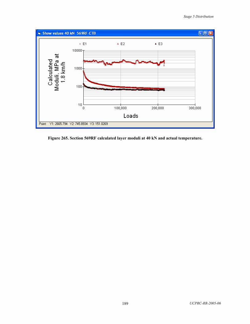
Stage 5 Distribution
UCPRC-RR-2005-06 189
Figure 265. Section 569RF calculated layer moduli at 40 kN and actual temperature.

Stage 5 Distribution
UCPRC-RR-2005-06 190
6.8 Visual Cracking Versus Damage of the Top Asphalt Layer, Goal 9
In Figure 266, cracking at the surface of the pavement (in m/m2) is shown as a function of the calculated relative decrease in modulus of the AC layer.
MB road (Goal 9)
0
1
2
3
4
5
6
7
8
9
0 0.2 0.4 0.6 0.8 1
dE/Ei
Cra
ckin
g, m
/m2 567RF
568RF573RF571RF572RF569RF
Figure 266. Cracking versus relative decrease in modulus of AC layer for Goal 9 (MB road).
Cracking versus relative deflection
0
1
2
3
4
5
6
7
8
9
1 1.2 1.4 1.6 1.8 2 2.2 2.4 2.6
Deflection/initial deflection (RSD)
Cra
ckin
g m
/m2 567RF
568RF573RF571RF572RF569RF
Figure 267. Goal 9 (MB road), Cracking versus increase in deflection (RSD)
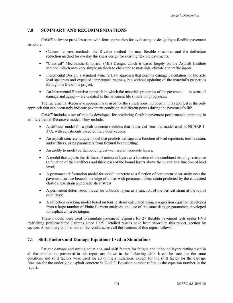
Stage 5 Distribution
UCPRC-RR-2005-06 191
7.0 SUMMARY AND RECOMMENDATIONS
CalME software provides users with four approaches for evaluating or designing a flexible pavement structure:
• Caltrans’ current methods: the R-value method for new flexible structures and the deflection reduction method for overlay thickness design for existing flexible pavements.
• “Classical” Mechanistic-Empirical (ME) Design, which is based largely on the Asphalt Institute Method, which uses very simple methods to characterize materials, climate and traffic inputs.
• Incremental Design, a standard Miner’s Law approach that permits damage calculation for the axle load spectrum and expected temperature regimes, but without updating of the material’s properties through the life of the project.
• An Incremental-Recursive approach in which the materials properties of the pavement — in terms of damage and aging — are updated as the pavement life simulation progresses.
The Incremental-Recursive approach was used for the simulations included in this report; it is the only approach that can accurately indicate pavement condition at different points during the pavement’s life.
CalME includes a set of models developed for predicting flexible pavement performance operating in an Incremental-Recursive model. They include:
• A stiffness model for asphalt concrete modulus that is derived from the model used in NCHRP 1-37A, with adjustments based on field observations;
• An asphalt concrete fatigue model that predicts damage as a function of load repetition, tensile strain, and stiffness, using parameters from flexural beam testing;
• An ability to model partial bonding between asphalt concrete layers;
• A model that adjusts the stiffness of unbound layers as a function of the combined bending resistance (a function of their stiffness and thickness) of the bound layers above them, and as a function of load level;
• A permanent deformation model for asphalt concrete as a function of permanent shear strain near the pavement surface beneath the edge of a tire, with permanent shear strain predicted by the calculated elastic shear strain and elastic shear stress
• A permanent deformation model for unbound layers as a function of the vertical strain at the top of each layer;
• A reflection cracking model based on tensile strain calculated using a regression equation developed from a large number of Finite Element analyses, and use of the same damage parameters developed for asphalt concrete fatigue.
These models were used to simulate pavement response for 27 flexible pavement tests under HVS trafficking performed for Caltrans since 1995. Detailed results have been shown in this report, section by section. A summary comparison of the results across all the sections of this report follows.
7.1 Shift Factors and Damage Equations Used in Simulations
Fatigue damage and rutting equations, and shift factors for fatigue and unbound layers rutting used in all the simulations presented in this report are shown in the following table. It can be seen that the same equations and shift factors were used for all of the simulations, except for the shift factor for the damage function for the underlying asphalt concrete in Goal 3. Equation number refers to the equation number in the report.

Stage 5 Distribution
UCPRC-RR-2005-06 192
Table 28. Summary of Damage Equations and Shift Factors Used in All Simulations
Fatigue Damage
Equation No.
Unbound Layers Rutting Equation No.
Fatigue Shift Factor
Unbound Layers Shift
Factor Goal 1 6 29 3 1 Goal 3 medium temp overlay
6 29 3 1
Goal 3 medium temp underlying
6 29 0.6 1
Goal 3 high temp 6 29 3 1 Goal 5 6 29 3 1 Goal 9 underlying 6 29 3 1
Parameter values for equations used in the simulations are presented in Section 9.4of this report.
7.2 Response Model
Resilient deflections were measured during 17 of the HVS tests. The deflections showed a considerable increase during the tests. For the Road Surface Deflectometer (RSD), the increase was between 38 and 304 percent, with an average value of 136 percent. The initial and final RSD deflections are shown in Table 29 and for the top MDD in Table 30.

Stage 5 Distribution
UCPRC-RR-2005-06 193
Table 29. Measured and Calculated Road Surface Deflectometer Deflections (RSD), in mm
RSD Measured Calculated Ratio Final/Initial
Section Initial Final Initial Final Measured Calculated
501RF 0.333 0.761 0.398 0.916 2.29 2.30
503RF 0.250 0.826 0.338 0.919 3.30 2.72
500RF 0.396 0.756 0.331 0.961 1.91 2.90
Goal 1
502CT 0.234 0.693 0.297 0.649 2.96 2.19
517RF 0.395 0.717 0.454 0.930 1.82 2.05
518RF 0.439 0.814 0.480 0.936 1.85 1.95
514RF 0.314 0.879 0.373 0.874 2.80 2.34
Goal 3,
20ºC
515RF 0.346 0.758 0.318 0.761 2.19 2.39
543RF 0.255 1.031 0.304 0.973 4.04 3.20
544RF 0.355 0.986 0.332 1.200 2.78 3.61
Goal 5
545RF 0.367 1.125 0.409 1.144 3.07 2.80
567RF 0.722 0.997 0.810 1.076 1.38 1.33
568RF 0.714 1.145 0.650 1.019 1.60 1.57
573RF 0.790 1.128 0.791 1.093 1.43 1.38
571RF 0.618 1.088 0.844 1.036 1.76 1.23
572RF 0.740 1.530 0.924 1.089 2.07 1.18
Goal 9
569RF 0.591 1.376 0.399 1.246 2.33 3.12

Stage 5 Distribution
UCPRC-RR-2005-06 194
Table 30. Measured and Calculated Deflections of the Top Multi-depth Deflectometer (MDD), in mm
MDD0 Measured Calculated Ratio Final/Initial
Section Initial Final Initial Final Measured Calculated
501RF 0.364 0.852 0.343 0.813 2.34 2.37
503RF 0.277 0.916 0.283 0.816 3.31 2.88
500RF 0.358 0.668 0.324 0.849 1.87 2.62
Goal 1
502CT 0.195 0.673 0.259 0.672 3.45 2.59
517RF 0.463 0.768 0.385 0.823 1.66 2.14
518RF 0.400 0.742 0.413 0.839 1.86 2.03
514RF 0.232 0.879 0.342 0.770 3.79 2.25
Goal 3,
20ºC
515RF 0.390 0.688 0.279 0.694 1.76 2.49
543RF 0.258 1.015 0.286 0.976 3.93 3.41
544RF 0.385 1.049 0.317 1.211 2.72 3.82
Goal 5
545RF 0.355 1.213 0.385 1.243 3.42 3.23
567RF 0.805 0.752 0.732 0.972 0.93 1.33
571RF 0.728 1.000 0.726 0.889 1.37 1.22
Goal 9
569RF 0..266 1.092 0.302 1.097 4.11 3.63
The test sections are listed in the tables in the same order that they are presented in the report. Variation in temperature of the AC and the position of the RSD will influence deflection, so the deflections are average values at the beginning and end of the HVS testing based on measurements at all RSD positions and uncorrected for the expected minor differences in temperature at time of measurement. All deflections were measured at the centerline of a 40 kN dual wheel load.
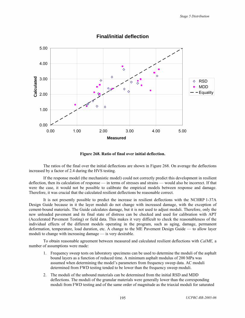
Stage 5 Distribution
UCPRC-RR-2005-06 195
Final/initial deflection
0.00
1.00
2.00
3.00
4.00
5.00
0.00 1.00 2.00 3.00 4.00 5.00
Measured
Cal
cula
ted
RSDMDDEquality
Figure 268. Ratio of final over initial deflection.
The ratios of the final over the initial deflections are shown in Figure 268. On average the deflections increased by a factor of 2.4 during the HVS testing.
If the response model (the mechanistic model) could not correctly predict this development in resilient deflection, then its calculation of response — in terms of stresses and strains — would also be incorrect. If that were the case, it would not be possible to calibrate the empirical models between response and damage. Therefore, it was crucial that the calculated resilient deflections be reasonable correct.
It is not presently possible to predict the increase in resilient deflections with the NCHRP 1-37A Design Guide because in it the layer moduli do not change with increased damage, with the exception of cement-bound materials. The Guide calculates damage, but it is not used to adjust moduli. Therefore, only the new unloaded pavement and its final state of distress can be checked and used for calibration with APT (Accelerated Pavement Testing) or field data. This makes it very difficult to check the reasonableness of the individual effects of the different models operating in the program, such as aging, damage, permanent deformation, temperature, load duration, etc. A change to the ME Pavement Design Guide — to allow layer moduli to change with increasing damage — is very desirable.
To obtain reasonable agreement between measured and calculated resilient deflections with CalME, a number of assumptions were made:
1. Frequency sweep tests on laboratory specimens can be used to determine the moduli of the asphalt bound layers as a function of reduced time. A minimum asphalt modulus of 200 MPa was assumed when determining the model’s parameters from frequency sweep data. AC moduli determined from FWD testing tended to be lower than the frequency sweep moduli.
2. The moduli of the unbound materials can be determined from the initial RSD and MDD deflections. The moduli of the granular materials were generally lower than the corresponding moduli from FWD testing and of the same order of magnitude as the triaxial moduli for saturated
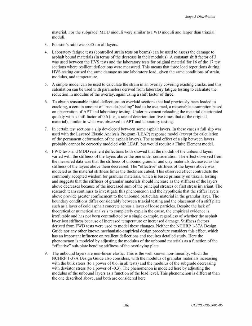
Stage 5 Distribution
UCPRC-RR-2005-06 196
material. For the subgrade, MDD moduli were similar to FWD moduli and larger than triaxial moduli.
3. Poisson’s ratio was 0.35 for all layers.
4. Laboratory fatigue tests (controlled strain tests on beams) can be used to assess the damage to asphalt bound materials (in terms of the decrease in their modulus). A constant shift factor of 3 was used between the HVS tests and the laboratory tests for original material for 16 of the 17 test sections where resilient deflections were measured. This means that three load repetitions during HVS testing caused the same damage as one laboratory load, given the same conditions of strain, modulus, and temperature.
5. A simple model can be used to calculate the strain in an overlay covering existing cracks, and this calculation can be used with parameters derived from laboratory fatigue testing to calculate the reduction in modulus of the overlay, again using a shift factor of three.
6. To obtain reasonable initial deflections on overlaid sections that had previously been loaded to cracking, a certain amount of “pseudo-healing” had to be assumed, a reasonable assumption based on observation of APT and laboratory testing. Under pavement reloading the material deteriorated quickly with a shift factor of 0.6 (i.e., a rate of deterioration five times that of the original material), similar to what was observed in APT and laboratory testing.
7. In certain test sections a slip developed between some asphalt layers. In these cases a full slip was used with the Layered Elastic Analysis Program (LEAP) response model (except for calculation of the permanent deformation of the asphalt layers). The actual effect of a slip between layers probably cannot be correctly modeled with LEAP, but would require a Finite Element model.
8. FWD tests and MDD resilient deflections both showed that the moduli of the unbound layers varied with the stiffness of the layers above the one under consideration. The effect observed from the measured data was that the stiffness of unbound granular and clay materials decreased as the stiffness of the layers above them decreased. The “effective” stiffness of the layers above was modeled as the material stiffness times the thickness cubed. This observed effect contradicts the commonly accepted wisdom for granular materials, which is based primarily on triaxial testing and suggests that the stiffness of granular materials should increase as the stiffness of the layers above decreases because of the increased sum of the principal stresses or first stress invariant. The research team continues to investigate this phenomenon and the hypothesis that the stiffer layers above provide greater confinement to the unbound particulate material in the granular layer. The boundary conditions differ considerably between triaxial testing and the placement of a stiff plate such as a layer of cold asphalt concrete across a layer of loose particles. Despite the lack of theoretical or numerical analysis to completely explain the cause, the empirical evidence is irrefutable and has not been contradicted by a single example, regardless of whether the asphalt layer lost stiffness because of increased temperature or increased damage. Stiffness factors derived from FWD tests were used to model these changes. Neither the NCHRP 1-37A Design Guide nor any other known mechanistic-empirical design procedure considers this effect, which has an important influence on resilient deflections and requires detailed study. Here the phenomenon is modeled by adjusting the modulus of the unbound materials as a function of the “effective” sub-plate bending stiffness of the overlaying plate.
9. The unbound layers are non-linear elastic. This is the well known non-linearity, which the NCHRP 1-37A Design Guide also considers, with the modulus of granular materials increasing with the bulk stress (to a power of 0.6, in all tests) and the modulus of the subgrade decreasing with deviator stress (to a power of -0.3). The phenomenon is modeled here by adjusting the modulus of the unbound layers as a function of the load level. This phenomenon is different than the one described above, and both are considered here.
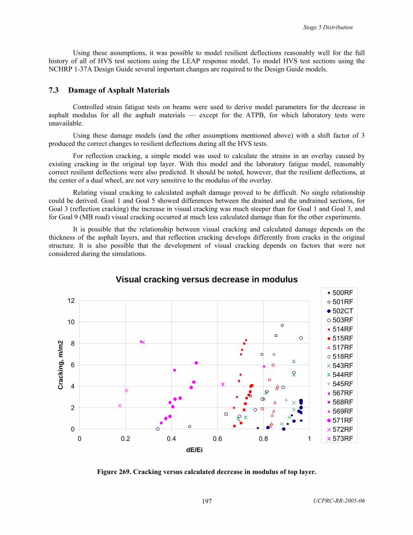
Stage 5 Distribution
UCPRC-RR-2005-06 197
Using these assumptions, it was possible to model resilient deflections reasonably well for the full history of all of HVS test sections using the LEAP response model. To model HVS test sections using the NCHRP 1-37A Design Guide several important changes are required to the Design Guide models.
7.3 Damage of Asphalt Materials
Controlled strain fatigue tests on beams were used to derive model parameters for the decrease in asphalt modulus for all the asphalt materials — except for the ATPB, for which laboratory tests were unavailable.
Using these damage models (and the other assumptions mentioned above) with a shift factor of 3 produced the correct changes to resilient deflections during all the HVS tests.
For reflection cracking, a simple model was used to calculate the strains in an overlay caused by existing cracking in the original top layer. With this model and the laboratory fatigue model, reasonably correct resilient deflections were also predicted. It should be noted, however, that the resilient deflections, at the center of a dual wheel, are not very sensitive to the modulus of the overlay.
Relating visual cracking to calculated asphalt damage proved to be difficult. No single relationship could be derived. Goal 1 and Goal 5 showed differences between the drained and the undrained sections, for Goal 3 (reflection cracking) the increase in visual cracking was much steeper than for Goal 1 and Goal 3, and for Goal 9 (MB road) visual cracking occurred at much less calculated damage than for the other experiments.
It is possible that the relationship between visual cracking and calculated damage depends on the thickness of the asphalt layers, and that reflection cracking develops differently from cracks in the original structure. It is also possible that the development of visual cracking depends on factors that were not considered during the simulations.
Visual cracking versus decrease in modulus
0
2
4
6
8
10
12
0 0.2 0.4 0.6 0.8 1
dE/Ei
Cra
ckin
g, m
/m2
500RF501RF502CT503RF514RF515RF517RF518RF543RF544RF545RF567RF568RF569RF571RF572RF573RF
Figure 269. Cracking versus calculated decrease in modulus of top layer.

Stage 5 Distribution
UCPRC-RR-2005-06 198
No single relationship could be established between the relative increase in deflection and the amount of surface cracking, Figure 270, but it may be noted that visible cracking was not observed until the deflection had increased by 50 percent or more. For the pavements with thin asphalt layers (Sections 567RF–573RF) and for rehabilitated pavements (Sections 514RF-518RF) the relative increase in deflection is lower, 50–100 percent, than for the thicker, original pavements (Sections 500RF-503RF) where it is 100–200 percent. The largest increase in deflection is for the wet tests (Sections 543RF–545RF).
Cracking versus relative deflection
0
2
4
6
8
10
12
1 1.5 2 2.5 3 3.5 4 4.5
Deflection/initial deflection
Cra
ckin
g m
/m2
500RF501RF502CT503RF514RF515RF517RF518RF543RF544RF545RF567RF568RF569RF571RF572RF573RF
Figure 270. Cracking versus increase in deflection.
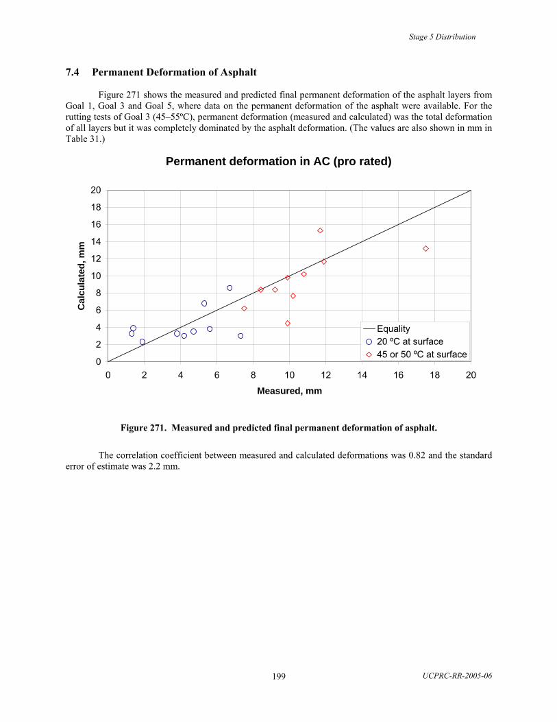
Stage 5 Distribution
UCPRC-RR-2005-06 199
7.4 Permanent Deformation of Asphalt
Figure 271 shows the measured and predicted final permanent deformation of the asphalt layers from Goal 1, Goal 3 and Goal 5, where data on the permanent deformation of the asphalt were available. For the rutting tests of Goal 3 (45–55ºC), permanent deformation (measured and calculated) was the total deformation of all layers but it was completely dominated by the asphalt deformation. (The values are also shown in mm in Table 31.)
Permanent deformation in AC (pro rated)
0
2
4
6
8
10
12
14
16
18
20
0 2 4 6 8 10 12 14 16 18 20
Measured, mm
Cal
cula
ted,
mm
Equality20 ºC at surface45 or 50 ºC at surface
Figure 271. Measured and predicted final permanent deformation of asphalt.
The correlation coefficient between measured and calculated deformations was 0.82 and the standard error of estimate was 2.2 mm.

Stage 5 Distribution
UCPRC-RR-2005-06 200
Table 31. Final Permanent Deformation of Asphalt, in mm
Section Measured Calculated Ratio =
Measured/Calculated
501RF 4.7 3.6 1.3
503RF 3.8 3.4 1.1
500RF 5.6 3.9 1.4
Goal 1
502CT 4.2 3.2 1.3
517RF 5.3 4.9 1.1
518RF 1.4 2.4 0.6
514RF 1.9 2.1 0.9
Goal 3, 20ºC
515RF 1.4 2.4 0.6
543RF 7.2 2.6 2.8 Goal 5
544RF 1.3 2.6 0.5
504RF 7.5 6.2 1.2
505RF 9.9 4.5 2.2
506RF 10.2 7.7 1.3
507RF 11.9 11.7 1.0
508RF 11.7 15.3 0.8
509RF 10.8 10.2 1.1
510RF 9.2 8.4 1.1
511RF 9.9 9.8 1.0
512RF 8.4 8.4 1.0
Goal 3, Rutting
(45– 55ºC)
513RF 17.5 13.2 1.3
The asphalt layers of Section 543RF, which was a wet drained test where the ATPB apparently collapsed, had a high measured permanent deformation. The permanent deformation was measured between elevation 0 mm and 250 mm, comprising 47 mm of the ATPB layer that may have caused the 4.6-mm difference between measured and calculated permanent deformation.

Stage 5 Distribution
UCPRC-RR-2005-06 201
The high temperature tests with the bias-ply dual tire and with the aircraft tire both resulted in smaller calculated than measured values.
7.5 Permanent Deformation of Granular Layers
The permanent deformation of the granular layers for Goal 1, Goal 3, and Goal 5 are shown in Figure 272. It should be noted that the permanent deformations are rather small, except for Section 543RF, the wet drained section, where the permanent deformation includes part of the ATPB, which completely stripped and collapsed after 600,000 repetitions (which the models cannot capture).
Permanent deformation of granular layers
0
2
4
6
8
10
12
14
0 2 4 6 8 10 12 14
Measured, mm
Cal
cula
ted,
mm
Goal 1Goal 3Goal 5Equality
Figure 272. Final permanent deformation of granular layers.
The scatter of the data is very large, as may be seen in the plots in this report. The average coefficient of variation is 58 percent. The measured values shown in Figure 272 are averages. The values are also shown (in mm) in Table 32.

Stage 5 Distribution
UCPRC-RR-2005-06 202
Table 32. Final Permanent Deformation of Granular Layer, in mm
Section Measured Calculated
501RF 3.4 3.7
503RF 6.1 4.5
500RF 3.1 5.8
Goal 1
502CT 2.8 2.7
517RF 3.5 1.4
518RF 1.5 0.9
514RF 2.3 0.3
Goal 3,
20ºC
515RF 0.5 0.5
543RF 12.6 2.7 Goal 5
544RF 4.7 3.4
For Goal 3 the predicted permanent deformations tended to underestimate the measured values. It is possible that some recovery from permanent deformation took place from Goal 1 to Goal 3. Assuming a full recovery, however, would have resulted in overpredictions of the deformations.
The permanent deformations of the granular materials were predicted using Equation (29) with the following parameters:
Table 33. Parameters used for Granular Materials in Equation (29)
Parameter Value
A 0.8 mm
α 0.333
respref 1000 μstrain
β 1.333
Eref 40 MPa
γ 0.333
Permanent deformation was calculated both at the top of the AB (aggregate base) and at the top of the ASB. The two materials are rather similar and might have been treated as a single layer. In that case, the parameter A should have been increased to 1.1 mm, the value used for the subgrade.

Stage 5 Distribution
UCPRC-RR-2005-06 203
7.6 Permanent Deformation of Subgrade
The final permanent deformation of the subgrade was even smaller than that of the granular layers, with a maximum measured value of less than 2 mm. In addition the scatter of the data was as large as for the granular layers, with an average coefficient of variation of 70 percent. This is far from ideal for the calibration of a permanent deformation model for the subgrade.
The mean measured and predicted final deformations are shown in Figure 273 and (in mm) Table 34.
Permanent deformation of subgrade
0.0
0.5
1.0
1.5
2.0
2.5
3.0
0.0 0.5 1.0 1.5 2.0 2.5 3.0
Measured, mm
Cal
cula
ted,
mm
Figure 273. Final permanent deformation of the subgrade.

Stage 5 Distribution
UCPRC-RR-2005-06 204
Table 34. Final Permanent Deformation of Subgrade, in mm
Section Measured Calculated
501RF 1.3 1.4
503RF 1.9 1.4
500RF 1.2 2.7
Goal 1
502CT 0.4 1.0
517RF 1.4 0.7
518RF 0.3 0.3
514RF 0.2 0.2
Goal 3,
20ºC
515RF 0.3 0.2
543RF 0.0 1.0 Goal 5
544RF 0.0 1.4
The permanent deformations of the subgrade were predicted using Equation (29 with the following
parameters: Table 35. Parameters Used for Subgrade in Equation (29)
Parameter Value
A 1.1 mm
α 0.333
respref 1000 μstrain
β 1.333
Eref 40 MPa
γ 0.333

Stage 5 Distribution
UCPRC-RR-2005-06 205
7.7 Total Permanent Deformation at Pavement Surface
Figure 274 shows the final calculated permanent deformation at the pavement surface versus the mean value of the measured final average deformation over the test area, determined from profile data. It should be noted that the permanent deformation often showed considerable variation over the test area, as also indicated by the minimum and maximum values shown in some of this report’s graphs.
Permanent deformation at pavement surface
0.0
5.0
10.0
15.0
20.0
0.0 5.0 10.0 15.0 20.0
Measured, mm
Cal
cula
ted,
mm
Goal 1 Goal 3 45/55°CGoal 3 20°C Goal 5Goal 9 Equality
Figure 274. Final permanent deformation at the pavement surface (profile data).
For the wet experiment in Goal 5, the predicted final deformation was underestimated for the drained Section 543RF because of the collapse of the ATPB layer after it stripped under heavy loading and large amounts of water drained through it.
The final permanent deformations are also shown (in mm) in Table 36.

Stage 5 Distribution
UCPRC-RR-2005-06 206
Table 36. Final Permanent Deformation at the Pavement Surface, in mm
Section Measured Calculated
500RF 12.3 12.8 501RF 9.0 7.2 502CT 9.5 9.5
Goal 1
503RF 8.1 9.0 504RF 7.5 6.2 505RF 9.9 4.5 506RF 10.2 7.7 507RF 11.9 11.7 508RF 11.7 15.3 509RF 10.8 10.2 510RF 9.2 8.4 511RF 9.9 9.8 512RF 8.4 8.4
Goal 3,
45-55ºC
513RF 17.5 13.2 514RF 4.6 2.9 515RF 3.9 3.9 517RF 6.3 8.8
Goal 3,
20ºC
518RF 3.3 3.2 543RF 13.7 7.5 544RF 10.7 13.4
Goal 5
Wet 545RF 5.4 1.8 567RF 5.5 5.1 568RF 6.7 7.5 569RF 3.6 5.6 571RF 5.7 7.6 572RF 8.7 5.4
Goal 9
MB
road
573RF 7.0 9.7
The correlation coeficient between measured and calculated total permanent deformation was 0.61 and the standard error of estimate was 2.6 mm.

Stage 5 Distribution
UCPRC-RR-2005-06 207
7.8 Recommendations
The overall results from this study indicate that Incremental-Recursive models provide reasonable results when predicting the response and performance of pavements under HVS loading. However, now that the models have been shown to match the mechanics of the pavements under these conditions, additional work remains before the models can be used for pavement design and performance prediction.
There are significant differences between HVS testing and the field, and the approach used in this study has limitations because of those differences.
First, the effects of aging and of seasonal variations have not been quantified in the results included in this report because the models were calibrated using HVS tests of relatively short duration. Seasonal variation of unbound layers’ stiffness can be input in CalME by the user, and can be taken from typical patterns measured in the field. Aging and seasonal variation affect asphalt concrete stiffnesses at the same time that damage is occurring. Aging increases stiffness, although deflection measurements in the field show that the net effect of aging and damage is an overall decrease in stiffness with accumulating traffic loads. Field calibration is required to evaluate the difference in response between the field pavement and the incremental-recursive simulation that should be attributed to aging. It is likely that the effect of aging can be dealt with through shift factors.
Second, neither the effects of rest periods between loadings nor of faster traffic have been included in the calibration. It is expected that rest periods and different trafficking patterns will result in different shift factors.
Third, moduli from frequency sweep data, triaxial tests, FWD tests, and MDD deflections used in this study are similar but not identical. The NCHRP 1-37A study proposes relying primarily on triaxial testing to characterize stiffnesses for flexible pavement layers and for permanent deformation parameters for asphaltic materials. Because the majority of work to be performed by Caltrans over the next several decades will involve rehabilitation and reconstruction, with some addition of lane capacity, the research team recommends that the most practical and economical methods for characterizing materials for Caltrans will be:
1. Backcalculating stiffnesses of existing pavement layers using FWD data,
2. Using flexural frequency sweep data to develop master stiffness curves of new asphaltic materials and for default values of materials for which test data are already available,
3. Using flexural fatigue data for damage parameters, for fatigue and reflection cracking of new asphaltic materials, and for default values of materials for which test data are already available,
4. Using repeated shear test data for permanent deformation parameters for new asphaltic materials, or default values of materials for which test data are already available, and
5. Using default values from previous backcalculation for stiffnesses of new unbound layers based on soil classification and achievement of required compaction.
Use of these methods to predict stiffnesses in field pavements in order to simulate field pavements needs to be evaluated with the CalME Incremental-Recursive models.
Following are the recommended next steps to develop these models:
1. Perform a sensitivity analysis using “typical” values for properties and climate in the database established to date, and tie these results to CalME with the Classical (Asphalt Institute MS-1 equations), Incremental (Miner’s Law), and Incremental-Recursive methods to evaluate reasonableness of sensitivity.
2. Validate the recommended methods for characterizing flexible pavement materials, listed above, in conjunction with the models described in this report by comparing simulated and actual performance from mainline highway case studies and full-speed, test track data, such as WesTrack and NCAT track.

Stage 5 Distribution
UCPRC-RR-2005-06 208
3. Address the variability of the input parameters (moduli, thicknesses, traffic loading, etc.) and uncertainty on the damage models. It is expected that the sensitivity analyses will identify the most important variables controlling expected performance. Employing a Monte Carlo simulation using those critical variables is one possibility that should be explored. An alternative is to estimate typical variability of performance in the field by drawing on available literature, then incorporating a factor for the uncertainty of design life. The NCHRP 1-37A report takes this approach. Another possible alternative would be a combined approach that uses simulation for the truly unknown variables, including traffic and weather, and a statistically derived distribution for the within project variables created by variations in materials and construction.
4. Make final decisions regarding use of cemented layers in the flexible pavement structure, then calibrate. It is generally recommended that “semi-rigid” pavements, in which asphalt concrete is placed directly on cement-treated base (CTB) or lean concrete base (LCB), not be used because of the relatively quick reflection of shrinkage cracks. However, because Caltrans has used semi-rigid pavements in the past and they remain in the current design method, it is therefore important to have models for the response and performance of these layers. Models for fatigue and crushing of these materials can be evaluated using APT data from Louisiana and from field data taken at mainline sections in California. The models in the NCHRP 1-37A report can be the starting point for such a validation-and-calibration exercise.

Stage 5 Distribution
UCPRC-RR-2005-06 209
8.0 REFERENCES
1. Bejarano, M. O., Harvey, J. T., Ali, A., Mahama, D., Hung, D., and Preedonant, P. December 2001 (Revision December 2004). Performance of drained and undrained flexible pavement structures under wet conditions: Accelerated test data, test section 545, undrained. (Draft report prepared for the California Department of Transportation.) UC Pavement Research Center, Institute of Transportation Studies, University of California: Davis and Berkeley.
2. Bejarano, M. O., Harvey, J. T., Ali, A., Mahama, D., Hung, D., and Preedonant, P. December 2001 (Revision May 2004). Performance of drained and undrained flexible pavement structures under wet conditions: Test data from accelerated pavement test section 544, undrained. (Draft report prepared for the California Department of Transportation.) UC Pavement Research Center, Institute of Transportation Studies, University of California: Davis and Berkeley.
3. Bejarano, M. O., Harvey, J. T., Ali, A., Mahama, D., Hung, D., and Preedonant, P. March 2003. Performance of drained and undrained flexible pavement structures in accelerated loading under wet conditions. Summary Report, Goal 5 Partnered Pavement Performance Program. (Draft report prepared for the California Department of Transportation.) UC Pavement Research Center, Institute of Transportation Studies. University of California: Davis and Berkeley.
4. Bejarano, M. O., Harvey, J. T., Ali, A., Russo, M., Mahama, D., Hung, D., and Preedonant, P. December 2001 (Revision February 2004). Performance of drained and undrained flexible pavement structures under wet conditions: Test data from accelerated pavement test section 543, drained. (Draft report prepared for the California Department of Transportation.) UC Pavement Research Center, Institute of Transportation Studies, University of California: Davis and Berkeley.
5. Bejarano, M., Morton, B., and Scheffy, C. August 2005. Summary of construction activities and results from six initial accelerated pavement tests conducted on asphalt concrete pavement section for modified-binder overlay. (Draft report prepared for the California Department of Transportation.) UC Pavement Research Center, Institute of Transportation Studies, University of Califonia: Davis and Berkeley.
6. Deacon, J.A, Harvey, J.T., Guada, I., Popescu, L., and Monismith, C.L. 2002. Analytically based approach to rutting prediction. Transportation Research Record 1806. Washington D.C.
7. de Beer, M., and Fisher, C. 1997 Contact stresses of pneumatic tires measured with the vehicle-road surface pressure transducer array (VRSPTA) system. Report for the University of California at Berkeley (UCB) and the Nevada Automotive Test Center (NATC). Transportek, CSIR. Pretoria, South Africa.
8. Harvey, J. T., Bejarano, M., Fantoni, A., Heath, A., Shin, H. C. December 2000. Performance of Caltrans asphalt concrete and asphalt-rubber hot mix overlays at moderate temperatures: Accelerated pavement testing evaluation. Draft report prepared for the California Department of Transportation. UC Pavement Research Center, Institute of Transportation Studies, University of California: Berkeley and Davis.
9. Harvey, J., Coetzee, N., and Louw, L. November 1999. CAL/APT Program: Construction of the goal 3 overlays and recommendations for improved overlay performance in California. Report prepared for the California Department of Transportation. UC Pavement Research Center, CAL/APT Program, Institute of Transportation Studies, University of California: Davis and Berkeley.
10. Harvey, J. T., du Plessis, L., Long, F., Deacon, J. A., Guada, I., Hung, D. and Scheffy, C. June 1997. CAL/APT Program: Test results from accelerated pavement test on pavement structure containing asphalt treated permeable base (ATPB), section 500RF. Report No. RTA-65W485-3, prepared for

Stage 5 Distribution
UCPRC-RR-2005-06 210
the California Department of Transportation. UC Pavement Research Center, CAL/APT Program, Institute of Transportation Studies, University of California: Davis and Berkeley.
11. Harvey, J. T., du Plessis, L., Long, F., Shatnawi, S., Scheffy, C., Tsai, B-W., Guada, I., Hung, D., Coetzee, N., Reimer, M., and Monismith, C. L. June 1996. Initial CAL/APT Program: Site information, test pavement construction, pavement materials characterizations, initial CAL/APT test results, and performance estimates. Report no. RTA-65W485-3, prepared for the California Department of Transportation. UC Pavement Research Center, CAL/APT Program, Institute of Transportation Studies, University of California: Davis and Berkeley.
12. Harvey, J., Guada, I., and Long, F. 2000. Effects of material properties, specimen geometry, and specimen preparation variables on asphalt concrete tests for rutting. Asphalt Paving Technology 69: 236.
13. Harvey, J., Guada, I., Scheffy, C., Louw, L., Prozzi, J., and Hung, D. February 1998. CAL/APT Program: Test results from accelerated pavement test on pavement structure containing asphalt treated permeable base, section 502CT. Draft report submitted to California Department of Transportation. UC Pavement Research Center, CAL/APT Program, Institute of Transportation Studies, University of California: Davis and Berkeley.
14. Harvey, J., Hung, D., Prozzi, J., Louw, L., Scheffy, C., and Guada, I. December 1997. CAL/APT Program: Test results from accelerated pavement test on pavement structure containing untreated aggregate base, section 503RF. Draft report submitted to California Department of Transportation. UC Pavement Research Center, CAL/APT Program, Institute of Transportation Studies, University of California: Davis and Berkeley.
15. Harvey, J., Long, F., and Prozzi, J. A. 1999. Application of CAL/APT results to long life flexible pavement reconstruction. 1999 Accelerated Pavement Testing International Conference. Nevada: Reno.
16. Harvey, J. and Popescu, L. January 2000. Rutting of Caltrans asphalt concrete and asphalt-rubber hot mix under different wheels, tires, and temperatures: Accelerated pavement testing evaluation. Draft report prepared for California Department of Transportation. UC Pavement Research Center, CAL/APT Program, Institute of Transportation Studies, University of California: Dais and Berkeley.
17. Harvey, J., Prozzi, J., Deacon, D., Hung, D., Guada, I., du Plessis, L., Long, F., and Scheffy, C. April 1999. CAL/APT Program: Test results from accelerated pavement test on pavement structure containing aggregate base (AB), section 501RF. Report prepared for the California Department of Transportation. Pavement Research Center, CAL/APT Program, Institute of Transportation Studies, University of California: Davis and Berkeley.
18. Harvey, J. T., Roesler, J., Coetzee, N. F., and Monismith, C. L. June 2000. CAL/APT Program Summary Report: Six Year Period, 1994-2000. Report number FHWA/CA/RM-2000/15. Prepared for California Department of Transportation. UC Pavement Research Center, CAL/APT Program, Institute of Transportation Studies, University of California: Davis and Berkeley.
19. Harvey, J., Tsai, B-W., Long, F., and Hung, D. June 1999. CAL/APT Program: Asphalt treated permeable base (ATPB), laboratory tests, performance predictions and evaluation of Caltrans and other agencies’ experience. Report prepared for the California Department of Transportation. UC Pavement Research Center, CAL/APT Program, Institute of Transportation Studies, University of California: Davis and Berkeley.
20. Hornych, P. and Gérard, A. January 1999. A pneumatic repeated load triaxial apparatus for unbound granular materials and subgrade soils. Proceedings of an International Workshop on Modelling and Advanced Testing for Unbound Granular Materials. Gomes Correia, A. and Balkema, A.A., eds. Lisbon.

Stage 5 Distribution
UCPRC-RR-2005-06 211
21. National Cooperative Highway Research Program (NCHRP). July 1985. Proposed AASHTO Guide for Design of Pavement Structures. Project 20-7/24.
22. National Cooperative Highway Research Program (NCHRP). March 2004. Guide for Mechanistic-Empirical Design of New and Rehabilitated Pavement Structures. National Cooperative Highway Research Program, Report 1-37A.
23. Tsai, B., Harvey, J., and Monismith, C. 2002. WesTrack Fatigue Performance Prediction Using Miner’s Law. Transportation Research Record 1809: 137–147.
24. Tsai, B., Harvey, J., and Monismith, C. 2002. High Temperature Fatigue and Fatigue Damage Process of Aggregate-Asphalt Mixes. Asphalt Paving Technology: Vol. 71, pp 345-385.
25. Ullidtz, P. 2002. Analytical tools for pavement design. Proceedings of the Ninth International Conference on Asphalt Pavements. Copenhagen.
26. Ullidtz, P. 2005. A Simple Model for Pavement Damage. Paper accepted for publication by the Transportation Research Board, National Research Council, Washington, D.C., 2005.
27. Wu, R-Z. 2005. Finite Element Analyses of Refective Cracking in Asphalt Concrete Overlays. Doctoral dissertation. Department of Civil and Environmental Engineering, University of California, Berkeley.
28. Tia, M., Rogue, R., Sirin, O. and Kim, H-J. 2002 “Evaluation of Superpave Mixtures with and without Polymer Modification by Means of Accelerated Pavement Testing.” Final report, University of Florida.

Stage 5 Distribution
UCPRC-RR-2005-06 212
9.0 APPENDIX
9.1 Glossary
A
Accelerated Pavement Testing (APT)
aggregate base (AB)
aggregate subbase (ASB)
asphalt concrete (AC)
asphalt rubber hot-mix gap-graded (ARHM-GG)
asphalt-treated permeable base (ATPB)
C
California Department of Transportation (Caltrans)
cement-treated base (CTB)
D
dense-graded asphalt concrete (DGAC)
Distinct Element Method (DEM)
E
Equivalent Single Axle Load (ESAL)
F
Falling Weight Deflectometer (FWD)
Finite Element Method (FEM)
Field Mix Field Compacted (FMFC)
H
Heavy Vehicle Simulator (HVS)

Stage 5 Distribution
UCPRC-RR-2005-06 213
L
Layered Elastic Analysis Program (LEAP)
lean concrete base (LCB)
ln logarithm to base e (natural logarithm)
log logarithm to base 10
M
Mechanistic-Empirical (ME)
Mechanistic-Empirical (ME) design
Mechanistic-Empirical Design Guide (MEPDG)
moisture content (MC)
modified binder (MB)
Multi-depth Deflectometer (MDD)
N
NCHRP 1-37A Design Guide (NCHRP 2004)
P
Pavement Management System (PMS)
R
Road Surface Deflectometer (RSD)
Repeated Simple Shear Tests at Constant Height (RSST-CH)
root-mean square (RMS)
S
sdf standard deviation factor (10 raised to the standard deviation of the logarithms of the values)
U
Unified Soil Classification System (USCS)
University of California Pavement Research Center (UCPRC)

Stage 5 Distribution
UCPRC-RR-2005-06 214
9.2 List of Units
ºC degree Celcius, centigrade
cm centimeter (0.001 m)
cPoise centi Poise (0.1 Pa×sec)
g/cm3 gram per cubic cm
Hz Hertz, oscillations per second
ºK degree Kelvin (as ºC but counted from absolute zero)
km/h kilometer per hour
kN kilo Newton (1,000 N)
kPa kilo Pascal (1,000 Pa)
MPa Mega Pascal (one million Pa)
msec millisecond
μstrain micro strain (10-6 m/m)
N Newton
ºR degree Rankine (as Fahrenheit but counted from absolute zero)
sec second
9.3 List of Parameters in Equations
α, β, γ, δ, λ, αA, αB, αC, αD, βA, βB, and βC are used to denote constants, which may be different from one
equation to another (in CalME forms the Greek letters are spelled alfa, beta, gamma, delta, and lambda)
γe elastic shear strain
γi inelastic (plastic) shear strain
θ bulk stress
σd deviator stress
τ shear stress
τoct octahedral shear stress
με strain in μstrain
ν Poisson’s ratio
ω damage
A constant in viscosity versus temperature relationship
aTg power on viscosity in reduced time relationship
C constant in non-linear modulus relation for cohesive soils
d deflection

Stage 5 Distribution
UCPRC-RR-2005-06 215
E modulus
EAC modulus of AC
Ei initial modulus (with no damage), or modulus of layer i
Emax maximum modulus
Emin minimum modulus
Eo modulus of unbound layer at reference stiffness of above layers
E40 kN modulus at a wheel load of 40 kN
EP modulus at a wheel load of P
hi thickness of layer i
I1 first stress invariant
J2 second deviator stress invariant
K calibration factor between rut depth and inelastic shear strain
k1, k2, and k3 constants in non-linear relation for unbound materials
lt loading time, corresponding to creep test
MN number of load applications in million
N number of load applications
n power in non-linear modulus relation for cohesive soils
P wheel load
p mean normal stress (I1/3 = θ/3)
pa atmospheric pressure
q mean deviator stress
respref reference response
rdAC rut depth in AC
S stiffness
Sref reference stiffness
SR stiffness ratio (E/Ei)
tr reduced time
visc viscosity
viscref viscosity at reference temperature
VTS viscosity temperature susceptibility
w internal energy density

Stage 5 Distribution
UCPRC-RR-2005-06 216
9.4 Parameter Values Used in Simulations
Master curve log(E)=delta+alfa/(1+exp(beta+gamma*log(tr)))
Reference temperature 20°C, frequency sweep data. Viscosity parameters A = 9.6307 (in ºK) and
VTS = -3.5047.
Name E delta E beta E gamma aT g Reference modulus
ATPB 2.3010 -0.2400 1.0000 1.0000 1144 DGAC-G1-Bot 2.3010 -0.4007 0.9807 1.2824 11172 DGAC-G1-Top 2.3010 -0.3987 0.9436 1.3529 9038 DGAC-G3 2.3010 -0.1790 0.8840 1.1770 7653 DGAC-G9 2.3010 -0.3032 0.8931 1.3370 7371 RAC-G 2.3010 -0.0841 0.9890 1.0080 4755
Fatigue and unbound layers rutting parameters
dam = A*MN^alfa*(eps/200)^beta*(E/3000)^gamma*exp(delta*t)
where dam is the damage, either fatigue damage or vertical rut depth.
Name Ft A Ft alfa Ft beta Ft
gamma Ft delta DGAC-G1-Top 0.001536 0.8695 4.1968 2.0984 0.1619 DGAC-G1-Bot 0.001245 0.8399 3.9718 1.9859 0.1913 DGAC-G3 0.008700 0.6874 3.2920 1.6460 0.1453 DGAC-G9 0.007357 0.4945 2.0612 1.0306 0.1263 RAC-G 0.018560 0.5911 2.9198 1.4599 0.1371
For the permanent deformation of the unbound layers the parameters were: A = 1.1 for subgrade and
0.8 for base and subbase, α = 0.333, Respref = 1000 μstrain instead of 200, β = 1.333, Eref = 40 MPa instead
of 3000, and γ = 0.333.
Permanent deformation of asphalt concrete
For Goal 1 and Goal 3 simulations a Gamma function was used, with parameters shown below.
Name Pd A Pd alfa Pd beta Pd
gamma DGAC-G1-Top -1.316 5.218 1.03 2.86DGAC-G1-Bot -1.316 5.218 1.03 2.86DGAC-G3 -0.568 4.208 1.03 2.47
For Goal 9 a power function was used:
rd = 7*layer thickness mm*MN^0.208*exp(1.03*shear stress/0.1 MPa)*elastic shear strain.

Stage 5 Distribution
UCPRC-RR-2005-06 217
9.5 Section 569RF Simulated with a CTB Model from an HVS Nordic Experiment.
In the Goal 9 experiments the aggregate base was 100 percent recycled material with a high content of recycled portland cement concrete. The backcalculated moduli of the base layer were shown in Figure 226, which has been reproduced below for convenience.
MB road, AB modulus
0.0
200.0
400.0
600.0
800.0
1000.0
1200.0
1400.0
7/1/2001 12/30/2001 7/1/2002 12/31/2002 7/1/2003
Date
Mod
ulus
, MPa
Figure 275. Modulus of AB layer backcalculated from FWD tests in center line.
The HVS test on Section 569RF was carried out from 03/25/2003 to 04/07/2003. During this period the backcalculated modulus of the AB was between 800 MPa and 1,200 MPa. Such a high modulus must be due to self-cementing of the layer. During the HVS test the surface deflection dropped rapidly, indicating that it might be necessary to simulate the layer as a lightly cemented aggregate base.
An incremental-recursive model for cement-treated base (CTB) materials was developed by C. Busch (Thogersen et al. 2004). The model is based on six HVS tests carried out in Southern Sweden using the HVS Nordic equipment, on three different CTB materials. Replicate sections were available for each material and one of the sections, for each material, was instrumented with stress and strain gauges for monitoring the response during the test. FWD tests were carried out before and after the tests and LWD (Light Weight Deflectometer) tests were done during the HVS testing. Two of the materials were based on a 0/16 mm gravel with target strengths (28 days, unconfined compressive) of 8 MPa and 4 MPa, respectively, and the third was based on a 0/8 mm sand, with a target strength of 4 MPa. The cement content ranged from 60 kg/m3 to 100 kg/m3. All materials had an addition of 331 kg/m3 of limestone powder.
The model developed is described as (quotation from page 41):

Stage 5 Distribution
UCPRC-RR-2005-06 218
With an initial CTB modulus assumed to be 1,000 MPa one gets β = 0.34 and γ = 0.14. The best agreement with the measured response was obtained using the α-value of 0.19 corresponding to the 25th percentile modulus. Equation 6 can then be written as:
14.034.019.0
100045 ⎟⎟⎠
⎞⎜⎜⎝
⎛×⎟⎟
⎠
⎞⎜⎜⎝
⎛−
×=MPa
Estrain
MNμμεω (34)
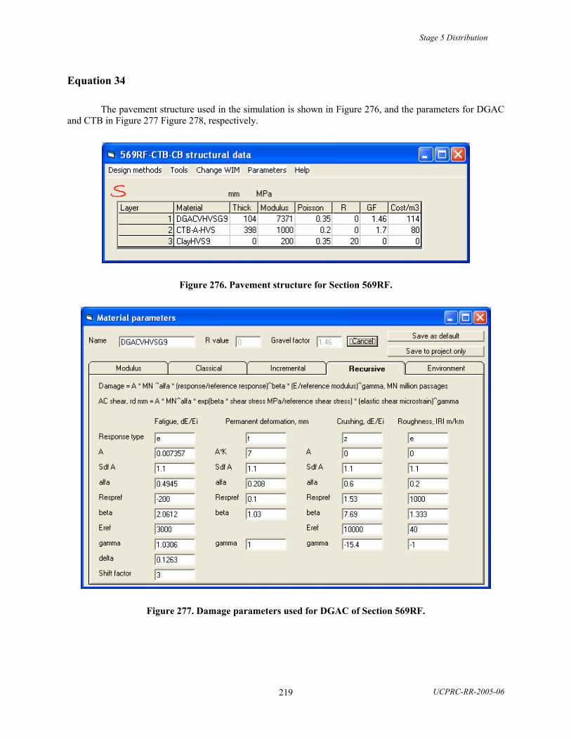
Stage 5 Distribution
UCPRC-RR-2005-06 219
Equation 34
The pavement structure used in the simulation is shown in Figure 276, and the parameters for DGAC and CTB in Figure 277 Figure 278, respectively.
Figure 276. Pavement structure for Section 569RF.
Figure 277. Damage parameters used for DGAC of Section 569RF.
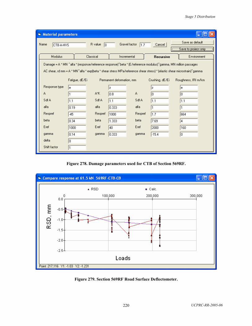
Stage 5 Distribution
UCPRC-RR-2005-06 220
Figure 278. Damage parameters used for CTB of Section 569RF.
Figure 279. Section 569RF Road Surface Deflectometer.
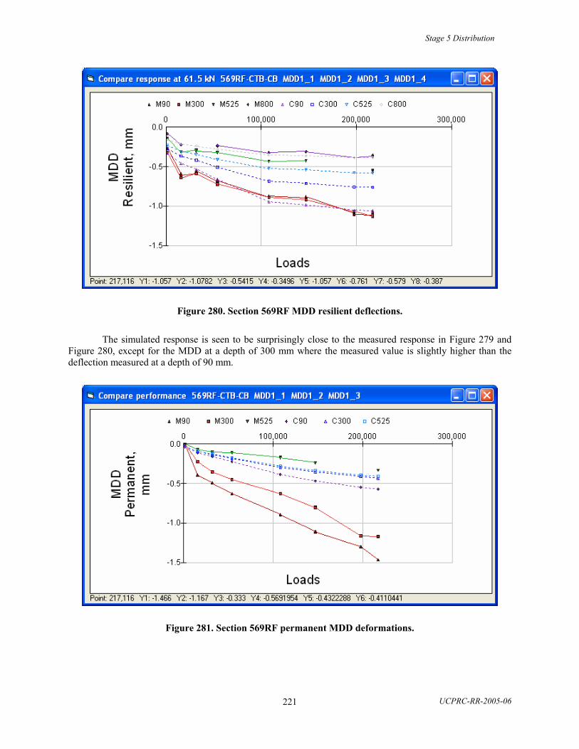
Stage 5 Distribution
UCPRC-RR-2005-06 221
Figure 280. Section 569RF MDD resilient deflections.
The simulated response is seen to be surprisingly close to the measured response in Figure 279 and Figure 280, except for the MDD at a depth of 300 mm where the measured value is slightly higher than the deflection measured at a depth of 90 mm.
Figure 281. Section 569RF permanent MDD deformations.

Stage 5 Distribution
UCPRC-RR-2005-06 222
Figure 282. Section 569RF average permanent deformation from pavement profile.
The permanent deformation on top of the CTB is underestimated whereas it is overestimated on the top of the asphalt, as shown in Figure 281 Figure 282. Had the gamma function derived for the Goal 3 DGAC for prediction of the AC permanent deformation been used instead of the power function, then the predicted permanent deformation of the asphalt would have been even larger.
Reference:
Thogersen, F., Busch, C., and Henrichsen, A. “Mechanistic Design of Semi-Rigid Pavements – An Incremental Approach,” Report 138, Danish Road Institute, 2004.
http://www.vejdirektoratet.dk/publikationer.asp?page=document&objno=73973