Calibration of a Magnetic Field Probe as aDiagnostic for Laser-Produced Plasma

L. A. Morton1∗1 Carson-Newman College, Jefferson City, TN 37760

E. T. Everson2,† C. G. Constantin2, D. Schaeffer2, P. Pribyl2, and C. Niemann2

2 University of California Los Angeles, Los Angeles, CA 90095

Small, high speed B-dot probes were constructed and calibrated as instruments to detect thespontaneous magnetic field of laser-produced plasma, following established techniques. A networkanalyzer and oscilloscopes were used to diagnose the source of interference observed both in thecalibration of the probes and in the laser-plasma measurements. Methods of reducing the interferencewere formulated, and tested when possible. A prototype analog integrator was also tested as areplacement for numerical integration of the probe signal. These improvements should allow moreaccurate magnetic field determinations for fast plasma phenomena using magnetic field probes.

PACS numbers:

I. INTRODUCTION

The magnetic field is an important property of aplasma, and knowledge of it is often needed to under-stand plasma behavior. There are varieties of ways todetect the magnetic field, but possibly the most straight-forward diagnostic is the use of a simple loop or coil ofwire. Faradays Law states:

V = −dΦB

dt= −aN dB⊥

dt(1)

where ΦB is the magnetic flux through the coil, B is theperpendicular component of the constant magnetic fieldstrength over the area of a coil, a is the coil area, N is thenumber of turns in the coil, and V is the electromotiveforce or voltage. By measuring the voltage across theleads of a coil, the time-derivative of the magnetic fluxthrough the coil can be determined. A B-dot probe isa plasma diagnostic instrument that takes advantage ofthis property. A B-dot probe usually consists of a single-or multi-turn coil mounted on or enclosed in a supportthat allows the coil to be inserted into or near the plasma.The term B-dot arises from the mathematical notationdBdt = B.1 The magnetic field itself can be determined

by integrating the B-dot signal in real-time by an analogintegrator circuit2,3 or numerically after digitization ofthe signal.4–6

For several reasons B-dot probes must be calibratedto achieve accurate field measurements. Since probestend to be small, physical measurements of the coil areaare inaccurate.7 In addition, non-ideal electronic effectstake place, especially involving the self-inductance of thecoil or the cabling.8 Calibration is often accomplishedby applying a known sinusoidal magnetic field from aHelmholtz coil driven by a signal generator and deter-mining the amplitude of probes response as a function offrequency using an oscilloscope.9 Alternatively a networkanalyzer can be used, which simplifies data collection andallows the phase of the probe’s response to be determinedas well.6–8,10

A. Probe Construction

For this report, probes were built using identical con-struction techniques as those described by Everson etal.6 The probe consists of two paired segments of magnetwire wrapped 5 times around each axis of a 3-axis heat-resistant plastic core, yielding coils of approximately 1mm diameter. The core is placed at the tip of an alu-mina shaft and covered by a glass capillary tube. Theleads from the loops are twisted into a bundle and runthe 8” length of the hollow shaft, terminating in connec-tions to six RG-178 coaxial cables. These carry the signalthrough the 3/8” stainless steel vacuum shaft and termi-nate in LEMO connectors that penetrate the vacuum seal(see Fig. 1).

FIG. 1: Wiring illustration of probe

The two loops on each axis are connected to their re-spective cables in the opposite sense so that a chang-ing magnetic flux will produce equal but opposite volt-ages from the two loops (Fig. 1). However, capacitativepickup will have the same polarity on each loop. There-fore, when the signals from the two loops are subtractedby the differential amplifier, the common capacitativevoltage will cancel, leaving the combined magneticallyinduced signal. Here Vmeas,1(t) and Vmeas,2(t) representthe opposite windings signals as functions of time, andC(t) represents the common capacitative signal:

Vmeas,1(t)−Vmeas,2(t) =(B + C(t)

)−(−B + C(t)

)= 2B(t)(2)

2

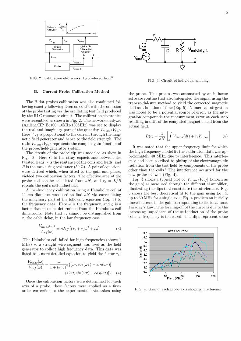
FIG. 2: Calibration electronics. Reproduced from6

B. Current Probe Calibration Method

The B-dot probes calibration was also conducted fol-lowing exactly following Everson et al6, with the omissionof the probe testing via the oscillating test field producedby the RLC resonance circuit. The calibration electronicswere assembled as shown in Fig. 2. The network analyzer(Agilent/HP E5100, 10kHz-180MHz) was set to displaythe real and imaginary part of the quantity Vmeas/Vref .Here Vref is proportional to the current through the mag-netic field generator and hence to the field strength. Theratio Vmeas/Vref represents the complex gain function ofthe probe/field-generator system.

The circuit of the probe tip was modeled as show inFig. 3. Here C is the stray capacitance between thetwisted leads, r is the resitance of the coils and leads, andR is the measuring resistance (50 Ω). A pair of equationswere derived which, when fitted to the gain and phase,yielded two calibration factors. The effective area of theprobe coil can be calculated from aN , and τs = L/Rreveals the coil’s self-inductance.

A low-frequency calibration using a Helmholtz coil of11 cm diameter was used to find aN via curve fittingthe imaginary part of the following equation (Eq. 3) tothe frequency data. Here ω is the frequency, and g is afactor that must be determined from the Helmholtz coildimensions. Note that τs cannot be distinguished fromτ , the cable delay, in the low frequency case.

Vmeas(ω)Vref (ω)

= aNg[(τs + τ)ω2 + iω

](3)

The Helmholtz coil failed for high frequencies (above 1MHz) so a straight wire segment was used as the fieldgenerator to collect high frequency data. This data wasfitted to a more detailed equation to yield the factor τs:

Vmeas(ω)Vref (ω)

=ω

1 + (ωτs)2[ωτscos(ωτ)− sin(ωτ)]

+i[ωτssin(ωτ) + cos(ωτ)] (4)

Once the calibration factors were determined for eachaxis of a probe, these factors were applied as a first-order correction to the experimental data taken using

FIG. 3: Circuit of individual winding

the probe. This process was automated by an in-housesoftware routine that also integrated the signal using thetrapezoidal-sum method to yield the corrected magneticfield as a function of time (Eq. 5). Numerical integrationwas noted to be a potential source of error, as the inte-gration compounds the measurement error at each stepresulting in drift of the computed magnetic field from theactual field.

B(t) =1aN

[∫Vmeas(dt) + τsVmeas

](5)

It was noted that the upper frequency limit for whichthe high-frequency model fit the calibration data was ap-proximately 40 MHz, due to interference. This interfer-ence had been ascribed to pickup of the electromagneticradiation from the test field by components of the probeother than the coils.6 The interference occurred for thenew probes as well (Fig. 4).

Fig. 4 shows a typical plot of |Vmeas/Vref | (known asthe gain) as measured through the differential amplifier,illustrating the dips that constitute the interference. Fig.5 shows the best theoretical fit to the gain using Eq. 4,up to 60 MHz for a single axis. Eq. 4 predicts an initiallylinear increase in the gain corresponding to the ideal case,Faraday’s Law. The leveling-off of the curve is due to theincreasing impedance of the self-induction of the probecoils as frequency is increased. The dips represent some

FIG. 4: Gain of each probe axis showing interference

3

FIG. 5: Best fit to calibration by IDL routine

other frequency-dependent reduction in the gain.This was the starting point for the current report.

Other calibration procedures using network analyzersseem to have encountered similar interference,7–9 in onecase at much higher frequency.1 Experiments were con-ducted to determine and remove the source of the infer-ence for this setup. An analog integrator was constructedand tested in hopes of eliminating numerical integrationand its accompanying uncertainty from the data analysis.The probes and the integrator were tested by measuringthe magnetic field of a laser-produced plasma. Interfer-ence was also seen in the experiment, and its source wastraced.

II. B-DOT CALIBRATION REFINEMENT

It was concluded that electromagnetic interferencefrom the magnetic source was not the cause, since thestray signal produced by positioning the wire segmentB-field source at the midpoint of the alumina shaft orthe steel shaft was not great enough in amplitude tocause such dips. Resonance of the inductance of thecoil and the capacitance of the twisted leads was an-other possible cause. However, the required capacitancevalue calculated to create a resonance at the observed fre-quencies, given the known inductance of the probe coils(≈ 2.5×107H), is unrealistically large (hundreds of nano-farads).

Impedance mismatching was then investigated as a po-tential cause of the interference. For transmission linessuch as coaxial cables, the cable has a characteristicimpedance Z that is substantially constant for all fre-quencies and cable lengths. In order to avoid the creationof standing waves or echoes in the cable, the devices con-nected at either end must have the same impedance.11Otherwise, a signal traveling through the cable will bereflected at the mismatch. However, no signal shouldarrive at the probe coils, since they are the only sourcein the circuit. Thus, impedance matching has not beenapplied to B-dot probe coils in prior works.

FIG. 6: Plot of frequency against dip number

The use of different cables and connection schemesdemonstrated that the interference was cable-related.The dips were evenly spaced in frequency, and this spac-ing depended on the cable configuration. Two differentsets of cable, differing in manufacturer and in length, buthaving the same impedance (50 Ω) were used betweenthe probe and the differential amplifier. For some testselectrical connection was made at the rear of the probebetween the LEMO connectors of the two cables com-prising a given axis (refer to Fig. 1). Shorting betweenthe bodies of two of these connectors creates an electri-cal connection between the external conductors of thetwo cables. Fig. 6 shows the results of the four possiblecombinations of conditions. The interference is clearlycable-dependent.

The evidence suggests that there is reflection occur-ring where the external cables connect to the differentialamplifier. Referring to Fig. 6, the frequency steps aresmaller for the connected case. Since wavelength and fre-quency are inversely proportional, this indicates a shortresonant cable length in the cross-connected case. Thisshorter length is independent of which external cable setwas used; the scope traces were nearly identical. Thus,the resonance is taking place in the internal cables ofthe probe when the cross-connection is made. When thecross-connection is not made, the entire cable assemblyresonates.

The external conductors of the cables are connectedto the (grounded) metal housing of the differential am-plifier. Making the cross-connection at the probe appar-ently moves the location of the reflection point. Thisimplies that the connection at the differential amplifieris causing a reflection. No resonance could occur if theimpedance mismatch were solely at the probe tip. Sincethe amplifier itself has 50 Ω input impedance, the prob-lem must lie with the BNC connectors on the cables. Re-placing these cables should remedy the reflection problemand allow accurate calibration up to 150 MHz.

Impedance matching at the probe tip should also elimi-nate the interference by preventing the reflections movingaway from the amplifier from being reflected back to theamplifier again. The resistance of a single coil was foundto be 3-5 Ω, whereas the cable had an impedance of 50Ω. A test probe was built with a single 47 Ω resistoradded in series with each coil. Using the inductance L

4

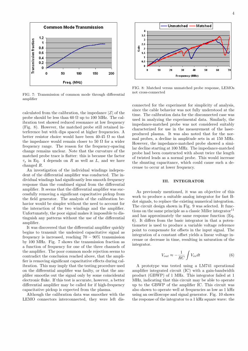
FIG. 7: Transmission of common mode through differentialamplifier

calculated from the calibration, the impedance |Z| of theprobe should be less than 60 Ω up to 100 MHz. The cal-ibration test showed reduced resonance at low frequency(Fig. 8). However, the matched probe still retained in-terference but with dips spaced at higher frequencies. Abetter resistor choice would have been 40-45 Ω so thatthe impedance would remain closer to 50 Ω for a widerfrequency range. The reason for the frequency-spacingchange remains unclear. Note that the curvature of thematched probe trace is flatter: this is because the factorτs in Eq. 4 depends on R as well as L, and we havechanged R.

An investigation of the individual windings indepen-dent of the differential amplifier was conducted. The in-dividual windings had significantly less smooth frequencyresponse than the combined signal from the differentialamplifier. It seems that the differential amplifier was suc-cessfully removing a significant capacitative pickup fromthe field generator. The analysis of the calibration be-havior would be simpler without the need to account forthe interaction of the two windings and the amplifier.Unfortunately, the poor signal makes it impossible to dis-tinguish any patterns without the use of the differentialamplifier.

It was discovered that the differential amplifier quicklybegins to transmit the undesired capacitative signal asfrequency is increased, reaching 70 − 90% transmissionby 100 MHz. Fig. 7 shows the transmission fraction asa function of frequency for one of the three channels ofthe amplifier. The poor common mode rejection seems tocontradict the conclusion reached above, that the ampli-fier is removing significant capacitative effects during cal-ibration. This may imply that the testing procedure usedon the differential amplifier was faulty, or that the am-plifier smooths out the signal only by some coincidentalelectronic fluke. If this test is accurate, however, a betterdifferential amplifier may be called for if high-frequencycapacitative pickup is expected from the plasma.

Although the calibration data was smoother with theLEMO connectors interconnected, they were left dis-

FIG. 8: Matched versus unmatched probe response, LEMOsnot cross-connected

connected for the experiment for simplicity of analysis,since the cable behavior was not fully understood at thetime. The calibration data for the disconnected case wasused in analyzing the experimental data. Similarly, theimpedance-matched probe was not considered suitablycharacterized for use in the measurement of the laser-produced plasma. It was also noted that for the nor-mal probes, a decline in amplitude sets in at 150 MHz.However, the impedance-matched probe showed a simi-lar decline starting at 100 MHz. The impedance-matchedprobe had been constructed with about twice the lengthof twisted leads as a normal probe. This would increasethe shunting capacitance, which could cause such a de-crease to occur at lower frequency.

III. INTEGRATOR

As previously mentioned, it was an objective of thiswork to produce a suitable analog integrator for fast B-dot signals, to replace the existing numerical integration.The circuit design shown in Fig. 9 was selected. It func-tions on the same principle as a classic Miller integrator11and has approximately the same response function (Eq.6). It differs from the basic integrator in that a poten-tiometer is used to produce a variable voltage referencepoint to compensate for offsets in the input signal. Theintegration of a constant offset yields a linear voltage in-crease or decrease in time, resulting in saturation of theintegrator.

Vout ≈ −1RC

∫Vindt (6)

A prototype was tested using a LM741 operationalamplifier integrated circuit (IC) with a gain-bandwidthproduct (GBWP) of 1 MHz. This integrator failed at 1MHz, indicating that this circuit may be able to operateup to the GBWP of the amplifier IC. This circuit wasalso shown to operate well at frequencies as low as 1 kHzusing an oscilloscope and signal generator. Fig. 10 showsthe response of the integrator to a 1 kHz square wave: the

5

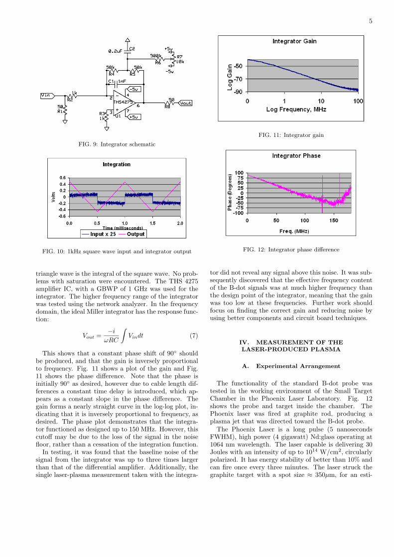
FIG. 9: Integrator schematic

FIG. 10: 1kHz square wave input and integrator output

triangle wave is the integral of the square wave. No prob-lems with saturation were encountered. The THS 4275amplifier IC, with a GBWP of 1 GHz was used for theintegrator. The higher frequency range of the integratorwas tested using the network analyzer. In the frequencydomain, the ideal Miller integrator has the response func-tion:

Vout =−iωRC

∫Vindt (7)

This shows that a constant phase shift of 90 shouldbe produced, and that the gain is inversely proportionalto frequency. Fig. 11 shows a plot of the gain and Fig.11 shows the phase difference. Note that the phase isinitially 90 as desired, however due to cable length dif-ferences a constant time delay is introduced, which ap-pears as a constant slope in the phase difference. Thegain forms a nearly straight curve in the log-log plot, in-dicating that it is inversely proportional to frequency, asdesired. The phase plot demonstrates that the integra-tor functioned as designed up to 150 MHz. However, thiscutoff may be due to the loss of the signal in the noisefloor, rather than a cessation of the integration function.

In testing, it was found that the baseline noise of thesignal from the integrator was up to three times largerthan that of the differential amplifier. Additionally, thesingle laser-plasma measurement taken with the integra-

FIG. 11: Integrator gain

FIG. 12: Integrator phase difference

tor did not reveal any signal above this noise. It was sub-sequently discovered that the effective frequency contentof the B-dot signals was at much higher frequency thanthe design point of the integrator, meaning that the gainwas too low at these frequencies. Further work shouldfocus on finding the correct gain and reducing noise byusing better components and circuit board techniques.

IV. MEASUREMENT OF THELASER-PRODUCED PLASMA

A. Experimental Arrangement

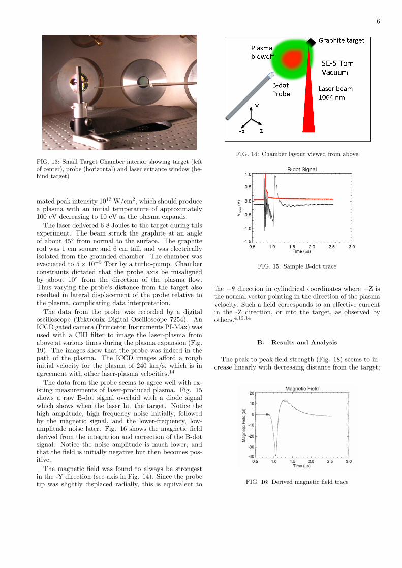
The functionality of the standard B-dot probe wastested in the working environment of the Small TargetChamber in the Phoenix Laser Laboratory. Fig. 12shows the probe and target inside the chamber. ThePhoenix laser was fired at graphite rod, producing aplasma jet that was directed toward the B-dot probe.

The Phoenix Laser is a long pulse (5 nanosecondsFWHM), high power (4 gigawatt) Nd:glass operating at1064 nm wavelength. The laser capable is delivering 30Joules with an intensity of up to 1014 W/cm2, circularlypolarized. It has energy stability of better than 10% andcan fire once every three minutes. The laser struck thegraphite target with a spot size ≈ 350µm, for an esti-

6

FIG. 13: Small Target Chamber interior showing target (leftof center), probe (horizontal) and laser entrance window (be-hind target)

mated peak intensity 1012 W/cm2, which should producea plasma with an initial temperature of approximately100 eV decreasing to 10 eV as the plasma expands.

The laser delivered 6-8 Joules to the target during thisexperiment. The beam struck the graphite at an angleof about 45 from normal to the surface. The graphiterod was 1 cm square and 6 cm tall, and was electricallyisolated from the grounded chamber. The chamber wasevacuated to 5× 10−5 Torr by a turbo-pump. Chamberconstraints dictated that the probe axis be misalignedby about 10 from the direction of the plasma flow.Thus varying the probe’s distance from the target alsoresulted in lateral displacement of the probe relative tothe plasma, complicating data interpretation.

The data from the probe was recorded by a digitaloscilloscope (Tektronix Digital Oscilloscope 7254). AnICCD gated camera (Princeton Instruments PI-Max) wasused with a CIII filter to image the laser-plasma fromabove at various times during the plasma expansion (Fig.19). The images show that the probe was indeed in thepath of the plasma. The ICCD images afford a roughinitial velocity for the plasma of 240 km/s, which is inagreement with other laser-plasma velocities.14

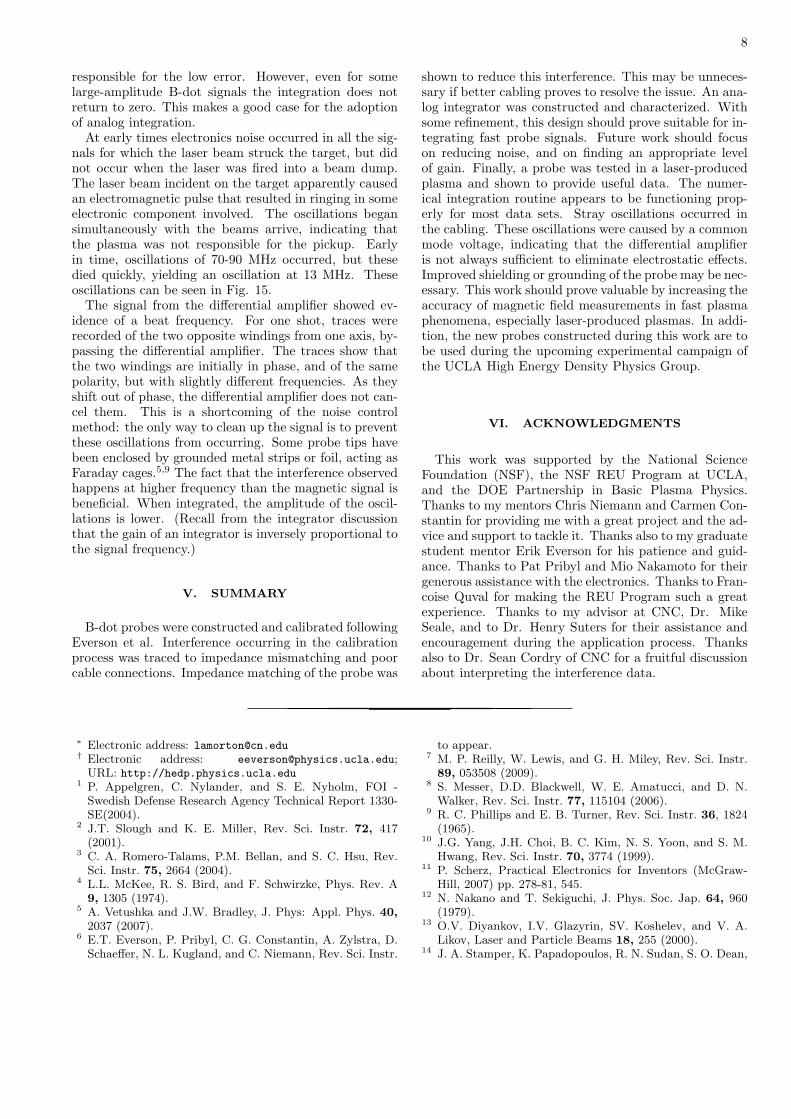
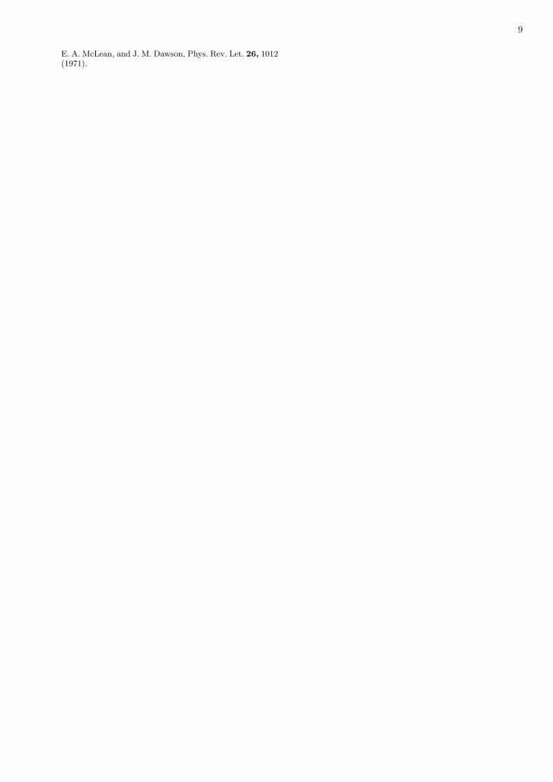
The data from the probe seems to agree well with ex-isting measurements of laser-produced plasma. Fig. 15shows a raw B-dot signal overlaid with a diode signalwhich shows when the laser hit the target. Notice thehigh amplitude, high frequency noise initially, followedby the magnetic signal, and the lower-frequency, low-amplitude noise later. Fig. 16 shows the magnetic fieldderived from the integration and correction of the B-dotsignal. Notice the noise amplitude is much lower, andthat the field is initially negative but then becomes pos-itive.

The magnetic field was found to always be strongestin the -Y direction (see axis in Fig. 14). Since the probetip was slightly displaced radially, this is equivalent to

FIG. 14: Chamber layout viewed from above

FIG. 15: Sample B-dot trace

the −θ direction in cylindrical coordinates where +Z isthe normal vector pointing in the direction of the plasmavelocity. Such a field corresponds to an effective currentin the -Z direction, or into the target, as observed byothers.4,12,14

B. Results and Analysis

The peak-to-peak field strength (Fig. 18) seems to in-crease linearly with decreasing distance from the target;

FIG. 16: Derived magnetic field trace

7

FIG. 17: Peak field arrival time versus distance

FIG. 18: Peak field strength versus distance

however, the last two points break this trend. This dis-crepancy may be due to inaccuracy of the probes radialplacement, or the fact that the plasma (and hence field)is confined to a narrower radius at shorter distances fromthe target. Fig. 19 shows this effect: the plasma expandsradially as it moves away from the target. The time de-lay between the laser firing and the peak magnetic fieldstrength was determined and plotted against the distanceof the probe from the target (Fig. 17). The slope of alinear fit to the data yields a speed of 140 km/s. This isin approximate agreement with the estimated 230 km/sinitial plasma speed, and with the fact that the magneticfield is frozen into the laser-plasma and travels with it.

A reversed field is observed after the peak field haspassed. Limited data from prior publications is availableon the shape of the magnetic probe signals. Nakano andSekiguchi, and Stamper et al, provide raw B-dot signaltraces.12,14 Unexpectedly, both bear a remarkable simi-larity to the shape of the integrated data from this exper-iment. If the inductance of a B-dot probe is great enough,it is possible for the B-dot to act in self-integrating modeat high frequencies.1,9 However, this is not likely to be thecase for the single-turn probe of Nakano and Sekiguchi.Some simulations and experiments do show that fieldreversal can occur.4,13 Since the numerical integrationseems to be working properly on these data sets, the re-versed field is considered to not to be an artifact.

FIG. 19: Time evolution of plasma, from successive lasershots. Target is in top right corner, B-dot probe is the diago-nal line. Note that the probe was translated between images

C. Evaluation of the Electronics

The numerical integration is relatively stable, espe-cially when the amplitude of the actual B-dot signal islarge. For traces with low B-dot signal (peak fields < 5Gauss), the noise and integration error prevented accu-rate field readings. In most other cases the integratedmagnetic field returned to a value close to zero, showingthat the cumulative integration error for these magneticfield traces was small. While the voltage resolution issmall (8-bit), the high sampling rate of the Tektronixoscilloscope (2.5 GS/s on each channel) is undoubtedly

8

responsible for the low error. However, even for somelarge-amplitude B-dot signals the integration does notreturn to zero. This makes a good case for the adoptionof analog integration.

At early times electronics noise occurred in all the sig-nals for which the laser beam struck the target, but didnot occur when the laser was fired into a beam dump.The laser beam incident on the target apparently causedan electromagnetic pulse that resulted in ringing in someelectronic component involved. The oscillations begansimultaneously with the beams arrive, indicating thatthe plasma was not responsible for the pickup. Earlyin time, oscillations of 70-90 MHz occurred, but thesedied quickly, yielding an oscillation at 13 MHz. Theseoscillations can be seen in Fig. 15.

The signal from the differential amplifier showed ev-idence of a beat frequency. For one shot, traces wererecorded of the two opposite windings from one axis, by-passing the differential amplifier. The traces show thatthe two windings are initially in phase, and of the samepolarity, but with slightly different frequencies. As theyshift out of phase, the differential amplifier does not can-cel them. This is a shortcoming of the noise controlmethod: the only way to clean up the signal is to preventthese oscillations from occurring. Some probe tips havebeen enclosed by grounded metal strips or foil, acting asFaraday cages.5,9 The fact that the interference observedhappens at higher frequency than the magnetic signal isbeneficial. When integrated, the amplitude of the oscil-lations is lower. (Recall from the integrator discussionthat the gain of an integrator is inversely proportional tothe signal frequency.)

V. SUMMARY

B-dot probes were constructed and calibrated followingEverson et al. Interference occurring in the calibrationprocess was traced to impedance mismatching and poorcable connections. Impedance matching of the probe was

shown to reduce this interference. This may be unneces-sary if better cabling proves to resolve the issue. An ana-log integrator was constructed and characterized. Withsome refinement, this design should prove suitable for in-tegrating fast probe signals. Future work should focuson reducing noise, and on finding an appropriate levelof gain. Finally, a probe was tested in a laser-producedplasma and shown to provide useful data. The numer-ical integration routine appears to be functioning prop-erly for most data sets. Stray oscillations occurred inthe cabling. These oscillations were caused by a commonmode voltage, indicating that the differential amplifieris not always sufficient to eliminate electrostatic effects.Improved shielding or grounding of the probe may be nec-essary. This work should prove valuable by increasing theaccuracy of magnetic field measurements in fast plasmaphenomena, especially laser-produced plasmas. In addi-tion, the new probes constructed during this work are tobe used during the upcoming experimental campaign ofthe UCLA High Energy Density Physics Group.

VI. ACKNOWLEDGMENTS

This work was supported by the National ScienceFoundation (NSF), the NSF REU Program at UCLA,and the DOE Partnership in Basic Plasma Physics.Thanks to my mentors Chris Niemann and Carmen Con-stantin for providing me with a great project and the ad-vice and support to tackle it. Thanks also to my graduatestudent mentor Erik Everson for his patience and guid-ance. Thanks to Pat Pribyl and Mio Nakamoto for theirgenerous assistance with the electronics. Thanks to Fran-coise Quval for making the REU Program such a greatexperience. Thanks to my advisor at CNC, Dr. MikeSeale, and to Dr. Henry Suters for their assistance andencouragement during the application process. Thanksalso to Dr. Sean Cordry of CNC for a fruitful discussionabout interpreting the interference data.

∗ Electronic address: lamorton@cn.edu† Electronic address: eeverson@physics.ucla.edu;

URL: http://hedp.physics.ucla.edu1 P. Appelgren, C. Nylander, and S. E. Nyholm, FOI -

Swedish Defense Research Agency Technical Report 1330-SE(2004).

2 J.T. Slough and K. E. Miller, Rev. Sci. Instr. 72, 417(2001).

3 C. A. Romero-Talams, P.M. Bellan, and S. C. Hsu, Rev.Sci. Instr. 75, 2664 (2004).

4 L.L. McKee, R. S. Bird, and F. Schwirzke, Phys. Rev. A9, 1305 (1974).

5 A. Vetushka and J.W. Bradley, J. Phys: Appl. Phys. 40,2037 (2007).

6 E.T. Everson, P. Pribyl, C. G. Constantin, A. Zylstra, D.Schaeffer, N. L. Kugland, and C. Niemann, Rev. Sci. Instr.

to appear.7 M. P. Reilly, W. Lewis, and G. H. Miley, Rev. Sci. Instr.

89, 053508 (2009).8 S. Messer, D.D. Blackwell, W. E. Amatucci, and D. N.

Walker, Rev. Sci. Instr. 77, 115104 (2006).9 R. C. Phillips and E. B. Turner, Rev. Sci. Instr. 36, 1824

(1965).10 J.G. Yang, J.H. Choi, B. C. Kim, N. S. Yoon, and S. M.

Hwang, Rev. Sci. Instr. 70, 3774 (1999).11 P. Scherz, Practical Electronics for Inventors (McGraw-

Hill, 2007) pp. 278-81, 545.12 N. Nakano and T. Sekiguchi, J. Phys. Soc. Jap. 64, 960

(1979).13 O.V. Diyankov, I.V. Glazyrin, SV. Koshelev, and V. A.

Likov, Laser and Particle Beams 18, 255 (2000).14 J. A. Stamper, K. Papadopoulos, R. N. Sudan, S. O. Dean,

9

E. A. McLean, and J. M. Dawson, Phys. Rev. Let. 26, 1012(1971).