Calibration and Validation of HEC-HMS Model for Chalakudy

_____________________________________________________________________________________________________ *Corresponding author: E-mail: [email protected];

International Journal of Environment and Climate Change 11(5): 91-104, 2021; Article no.IJECC.67689 ISSN: 2581-8627 (Past name: British Journal of Environment & Climate Change, Past ISSN: 2231–4784)

Calibration and Validation of HEC-HMS Model for Chalakudy River Basin

Gudidha Gopi1* and K. P. Rema2

1Department of Soil and Water Conservation Engineering, Kelappaji College of Agricultural

Engineering and Technology, KAU, Tavanur, Kerala, India. 2Department of Irrigation and Drainage Engineering, Kelappaji College of Agricultural Engineering and

Technology, KAU, Tavanur, Kerala, India.

Authors’ contributions

This work was carried out in collaboration between both authors. Author GG designed the study, run the model, performed the statistical analysis, managed the literature searcher, wrote the protocol and

wrote the first draft of the manuscript. Author KPR given the guidelines to complete HEC-HMS modelling, corrected the manuscript. Both authors read and approved the final manuscript.

Article Information

DOI: 10.9734/IJECC/2021/v11i530410

Editor(s): (1) Dr. Orlando Manuel da Costa Gomes, Lisbon Polytechnic Institute, Portugal.

(2) Dr. Daniele De Wrachien, State University of Milan, Italy. Reviewers:

(1) Andrei Urzică, Alexandru Ioan Cuza University, Romania. (2) Maruf Orewole, National Centre for Technology Management, Nigeria.

Complete Peer review History: https://www.sdiarticle4.com/review-history/67689

Received 12 March 2021 Accepted 19 May 2021

Published 14 July 2021

ABSTRACT

Prediction of flood prone areas in a basin and evolution of the impact of climate change on water resources needs a correct estimation of the availability of water which will solely be achieved by hydrological modelling of the basin. However, modelling the hydrology of a basin is a complex task and models should be well calibrated to increase user confidence in its predictive ability which in turn makes the application of the model effective. In this study rainfall-runoff simulation model viz., Hydrologic Modelling System, developed by the Hydrologic Engineering Centre USA (HEC-HMS) has been calibrated and validated for Chalakduy river basin in Kerala, in Sothern India for prediction of its hydrologic response. The result shows Curve Number (CN), Lag time and initial abstraction (Ia) to be the sensitive parameters for the simulated stream flow. The statistical analysis of Nash-Sutcliffe model efficiency criteria, the percentage error in peak, percentage error in volume, and net difference of observed and simulated time to peak, which were used for performance evaluation, have been found to range from (0.70 to 0.87), (4.39 to 19.47%), (1.9 to 19%) and (0 to 1day) respectively, indicating a very good performance of the model for simulation of stream flow.

Original Research Article

Gopi and Rema; IJECC, 11(5): 91-104, 2021; Article no.IJECC.67689

92

Keywords: Curve number (CN); hydrologic engineering centre and hydrologic modelling system (HEC-HMS); initial abstraction (Ia).

1. INTRODUCTION Globally floods are increasingly among the most devastating natural disasters affecting human life than any other natural disasters. According to Abhas, Jha, and Jessica (2012), in 2010 alone, 178 million people were affected by floods. It is also reported that one sixth of the global population (one billion people); the majority of them among the world's being low income earners live in the potential path of a 1 in 100 year flood according to Department for International Development (DFID). Extreme precipitation and floods are the hydro climatic events that draw considerable attention every year during the monsoon season in India. Millions of people are affected by extreme precipitation and flood events that often cause damage to infrastructure and agriculture in India. Extreme precipitation events have increased during the last few decades, which are likely to increase further under the warming climate (Goswami et al., 2006; Mukherjee et al., 2018; Roxy et al., 2017). India witnessed some of the most severe extreme precipitation and flood events during the recent decades. For instance, the extreme precipitation event in Mumbai in 2005 affected more than 20 million people and

caused more than 1000 deaths (Gupta and Nair, 2011). The 2013 extreme rainfall and flood event in Uttarakhand resulted in the death of more than 6000 people and caused an economic loss of more than $3.8 billion (Kumar, 2013). Furthermore, extreme precipitation in Chennai in November 2015 resulted in the economic loss of over $3 billion (Boyaj et al., 2018; Van Oldenborgh et al., 2016). Kerala with a total area of 38,863 km

2 is a state

in south India. Southwest and Northeast monsoons control the rainfall in Kerala. Kerala experiences 90% of rainfall during monsoon season. Chalakudy river basin chosen for the study was one among the worst affected basins in Kerala 2018 and 2019 flood events causing great loss to human beings and also resulted in damage of ground-works. In this study, the modeling of flood flows by calibration and validation of the basin simulation model, Hydrologic Modeling System, developed by the Hydrologic Engineering Center, USA (HEC-HMS) has been carried out for the Chalakudy river basin in Southern India for proper assessment and management of water resources in the basin.

Fig. 1. Location map of Chalakduy river basin

Outlet


93

1.1 Study Area

Chalakudy river is the fifth longest river in Kerala and drains through Palakkad, Thrissur and Ernakulam districts. The Chalakudy River Basin (CRB) lies between 10°05’ to 10°35’ North Lattitude and 76°15’ to 76°55’ East Longitude. The river originates from Anamalai hills of the Western Ghat mountain ranges and flows through the northern part of Periyar river after draining through varied physiographic and geologic terrains of Tamil Nadu and Kerala States. The basin receives an average rainfall of about 3000 mm. The total length of river is about 130 km and the catchment area is about 1370 km2. Out of the total catchment area, about 300 km

2 lies in Tamil Nadu and the remaining in

Kerala.

2. METHODOLOGY The hydrological simulation modelling was performed using HEC-HMS, which is a semi-distributed hydrologic model with the ability to perform continuous as well as event based simulation in dendritic watershed systems [1]. HEC-HMS is an advanced version of the HEC-1 model which was developed in 1968 by the US Army Corps of Engineers. Since then, HEC-HMS has been widely applied in hydrology to model the rainfall-runoff process, flood forecasting system planning and assessing impact of land-use changes and runoff simulations in ungauged basins [2] In HEC-HMS, the catchment is constructed by disintegrating the components of a hydrological cycle into manageable, elements viz. precipitation, initial abstraction, evapotranspiration, infiltration, surface runoff and base flow. In this model, the physical description of the watershed is described using elements, viz. sub-basin, reach, junction, reservoir, diversion, source and sink. Computation proceeds from upstream to downstream direction and calculation of runoff is carried out in a sequential manner starting from canopy storage through surface or depression storage, infiltration and transform into base flow/surface flow hydrograph. Rainfall is the major input to this model along with other spatially distributed watershed characteristics, such as land use/land cover and soil, and the output from the model is the flow hydrograph.

Different components included in the HEC-HMS are listed below.

• Basin Models: The physical basin area with hydrologic elements (sub basins, junctions, reach, reservoirs) and drainage network of the catchment are included in basin models.

• Meteorological Models: Information regarding meteorological components such as temperature, precipitation evapotranspiration, sunshine, humidity and snowmelt is defined in meteorological model. HEC-HMS provides variety of options to define each meteorological element.

• Control Specification: Starting date and time, ending date and time and computational time step for the simulation are defined in control specification.

• Time series Data: Real time series data for all the meteorological elements defined in meteorological model are fed in this part. Apart from above mentioned meteorological elements, discharge data can also be supplied for calibration and simulation of the developed model. It can be supplied to the software manually or in the form of HEC-DSS, the Hydrologic Engineering Center Data Storage System.

The data required for hydrologic modelling using (HEC-HMS) includes: i. Digital Elevation Model (DEM).ii. Land use iii. Soil map iv. Meteorological data v. Flow data.

2.1 Data Collection and Analysis a) Digital Elevation Model (DEM) For the present study, DEM of 30 m resolution downloaded from USGS earth explorer was used for delineating the basin and to decide basin characteristics such as elevation, slope, slope length, flow direction and drainage characteristics. b) Land use Land cover map The land use land cover map was prepared by using ERDAS Imagine 2014 software, which is available in the Geo Spatial lab of KCAET, Tavanur,Malappuram district,Kerala. Cloud Free Sentinel satellite data (geo coded with UTM projection, spheroid and datum WGS 1984, Zone 43 North) of 30m spatial resolution of the year (2020) has been downloaded from USGS Earth Explorer website (http://earthexplorer.usgs.gov/).


94

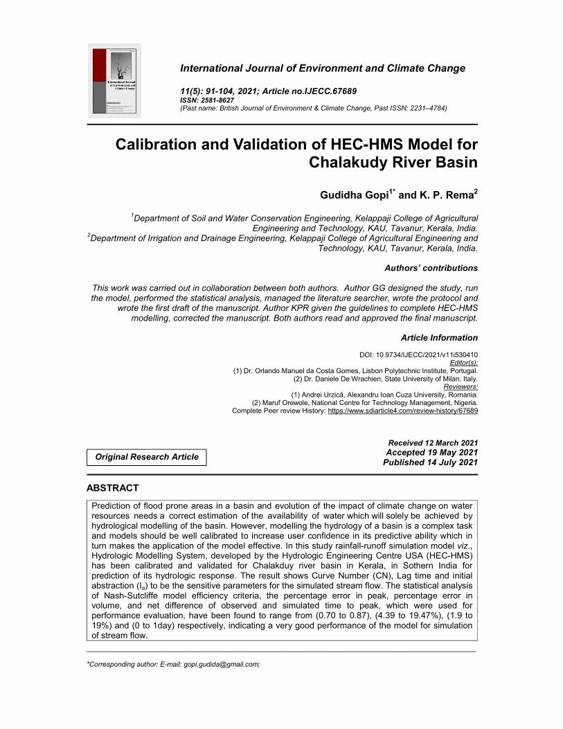
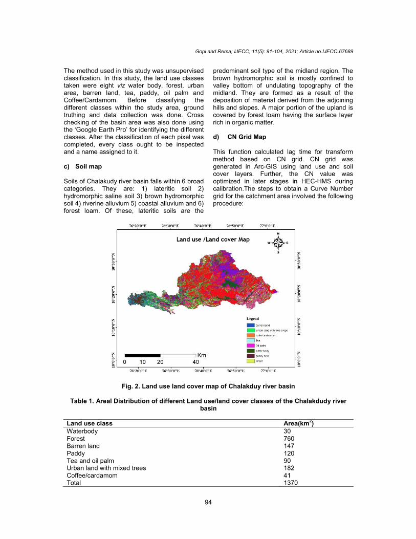
The method used in this study was unsupervised classification. In this study, the land use classes taken were eight viz water body, forest, urban area, barren land, tea, paddy, oil palm and Coffee/Cardamom. Before classifying the different classes within the study area, ground truthing and data collection was done. Cross checking of the basin area was also done using the ‘Google Earth Pro’ for identifying the different classes. After the classification of each pixel was completed, every class ought to be inspected and a name assigned to it. c) Soil map Soils of Chalakudy river basin falls within 6 broad categories. They are: 1) lateritic soil 2) hydromorphic saline soil 3) brown hydromorphic soil 4) riverine alluvium 5) coastal alluvium and 6) forest loam. Of these, lateritic soils are the

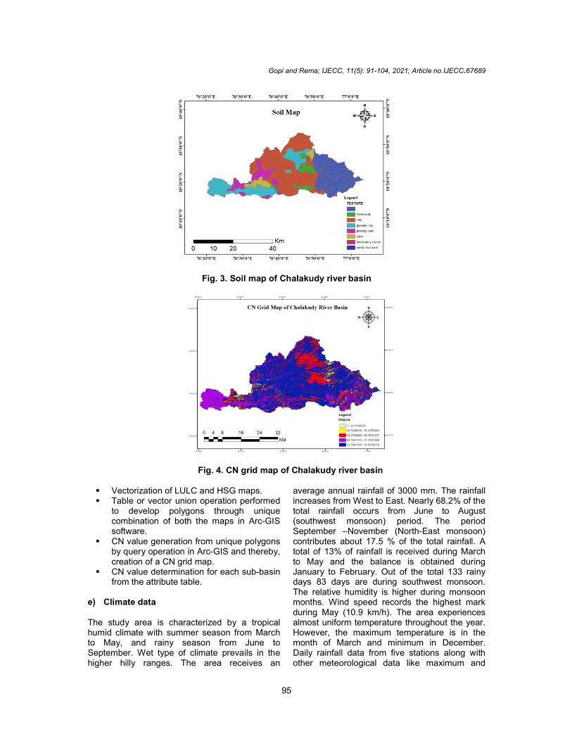
predominant soil type of the midland region. The brown hydromorphic soil is mostly confined to valley bottom of undulating topography of the midland. They are formed as a result of the deposition of material derived from the adjoining hills and slopes. A major portion of the upland is covered by forest loam having the surface layer rich in organic matter. d) CN Grid Map This function calculated lag time for transform method based on CN grid. CN grid was generated in Arc-GIS using land use and soil cover layers. Further, the CN value was optimized in later stages in HEC-HMS during calibration.The steps to obtain a Curve Number grid for the catchment area involved the following procedure:

Fig. 2. Land use land cover map of Chalakduy river basin

Table 1. Areal Distribution of different Land use/land cover classes of the Chalakdudy river basin

Land use class Area(km2) Waterbody 30 Forest 760 Barren land 147 Paddy 120 Tea and oil palm 90 Urban land with mixed trees 182 Coffee/cardamom 41 Total 1370


95

Fig. 3. Soil map of Chalakudy river basin

Fig. 4. CN grid map of Chalakudy river basin Vectorization of LULC and HSG maps. Table or vector union operation performed

to develop polygons through unique combination of both the maps in Arc-GIS software.

CN value generation from unique polygons by query operation in Arc-GIS and thereby, creation of a CN grid map.

CN value determination for each sub-basin from the attribute table.

e) Climate data The study area is characterized by a tropical humid climate with summer season from March to May, and rainy season from June to September. Wet type of climate prevails in the higher hilly ranges. The area receives an

average annual rainfall of 3000 mm. The rainfall increases from West to East. Nearly 68.2% of the total rainfall occurs from June to August (southwest monsoon) period. The period September –November (North-East monsoon) contributes about 17.5 % of the total rainfall. A total of 13% of rainfall is received during March to May and the balance is obtained during January to February. Out of the total 133 rainy days 83 days are during southwest monsoon. The relative humidity is higher during monsoon months. Wind speed records the highest mark during May (10.9 km/h). The area experiences almost uniform temperature throughout the year. However, the maximum temperature is in the month of March and minimum in December. Daily rainfall data from five stations along with other meteorological data like maximum and


96

minimum temperature, relative humidity, sunshine hours, wind speed etc., have been collected from ARS, Chalakudy and IMD, Pune.

f) Determination of average precipitation by Thiessen polygon method

Thiessen Polygon approach is the most sophisticated method in area-based weighting method, used in hydrometeorology for determining average rainfall when there is more than one observation station over a catchment area. Thiessen polygon map for calculating areal mean precipitation was prepared using the rainfall data from five rain gauge stations as shown in Fig.5. The weighted area of five gauging stations and their respective weightage of received rainfall over the basin is shown in Table 2.

2.2 HEC-HMS Hydrological Modelling

HEC-HMS uses separate models to represent each component of the runoff process, including models that compute runoff volume, models of

direct runoff, and models of base flow. Each model run combines a basin model, meteorological model and control specifications with run options to obtain results [3]. Following methods were selected for each component of runoff process such as runoff depth, direct runoff, base-flow and channel routing in event based hydrological modelling. These methods were selected on the basis of applicability and limitations of each method, availability of data, suitability for same hydrologic condition, well established, stable, widely acceptable, researcher recommendation etc.

I. SCS Curve Number (CN) method

In SCS-CN method, accumulated precipitation excess is estimated as a function of cumulative precipitation, soil cover, land use, and antecedent moisture and is:

Pe =(��)�

(��)

Table 2. Weighted area and weightage of different stations

SI. No. Gauging station Area (km2) Weights

1 Thunacadavu 137 0.107 2 Chalakudy 144 0.113 3 Peruvaripallam 230 0.18 4 Parambikulam 380 0.298 5 KSD 385 0.302

Fig. 5. Thiessen Polygon map for estimating areal mean precipitation

Table 3. Selected methods for HMS HMS Processes Method Loss SCS Curve Number Method Transform SCS Unit Hydrograph Base-flow Recession Routing Muskingum


97

Where, Pe = Accumulated precipitation excess at time t; P = Accumulated rainfall depth at time t; Ia = Initial abstraction and S = Potential maximum retention. Ia and S are calculated from following equations:

Ia = 0.2S

S=(��)

��

For a watershed that consists of several soil types and land uses, a composite CN is calculated as suggested by Panigrahi (2013). II. SCS unit hydrograph method SCS unit hydrograph method is applied for estimating direct runoff. The basin lag time (Tlag) is the parameter of SCS UH model which is 0.6 times the time of concentration (Tc), Value of Tc is computed as suggested by Panigrahi (2013). III. Recession method It is used to represent watershed base flow. It is given by:

Qt = Qo Rt

Where, Q0 = Initial base flow at time t = 0, Qt = Threshold flow at time t, and R = Exponential decay constant. Initial base flow (Qo) is estimated by field inspection. The recession constant (R) is estimated from observed flow hydrograph which depends upon the source of base flow. The threshold flow (Qt) is estimated from observed flows hydrograph, wherein the flow at which recession limb is approximated well by a straight line (USACE –HEC, 2008) [4]

IV. Muskingum method Muskingum method for channel routing was chosen. In this method X and K parameters must be evaluated. Theoretically, parameter K is the time of passing of a wave in reach length and parameter X is a constant coefficient whose value varies between 0 - 0.5. Therefore parameters can be estimated with the help of observed inflow and outflow hydrographs. Parameter K is estimated as the interval between similar points on the inflow and outflow hydrographs. Once K is estimated, X can be estimated by trial and error [4].

2.3 Calibration and Validation of Model Parameters

In the calibration procedure all the parameters involved were balanced in order to reduce the error between the observed values and the simulated values obtained for the basin [5]. It was mainly done to minimize the deviation between the observed and obtained values from the model and to get the best set of parameters in calibrating and validating the model [6]. The process was completed either by repeated manual adjustment of the parameters, computation and inspecting goodness of fit between the computed and observed hydrographs or automatically by using the iterative calibration procedure called optimization [7]. Daily available rainfall and discharge data from the year 2005 to 2007 were used for model calibration whereas the data from 2009 to 2010 were used for validation. The same parameters, obtained after calibration, were used for validation and thus the flood hydrographs of the catchment were generated.

2.4 Optimization of model parameters HEC-HMS itself provides a tool for optimization of the model parameters with user-defined numbers of iteration which is termed as the automatic calibration system. Different statistical evaluation parameters are also available in the model, in order to ensure the variation of calibrated results [8] 3. RESULTS AND DISCUSSION

3.1 Delineation of Chalakudy river basin The initial phase in building up HEC-GeoHMS project is terrain pre processing. Before starting the hydrologic modelling in the HEC-HMS software, the pre processing tool was used to derive eight datasets for stream and sub basin delineation. For carrying out the delineation procedure the HEC-GeoHMS extension tool in the Arc-Map was used [9]. The steps involved under pre processing menu are

a) Flow direction, b) Flow accumulation, c) Stream definition, d) Stream segmentation, e) Catchment grid delineation, f) Catchment polygon processing, g) Drainage line processing.


98

Fig. 6. Delineated Chalakudy river basin

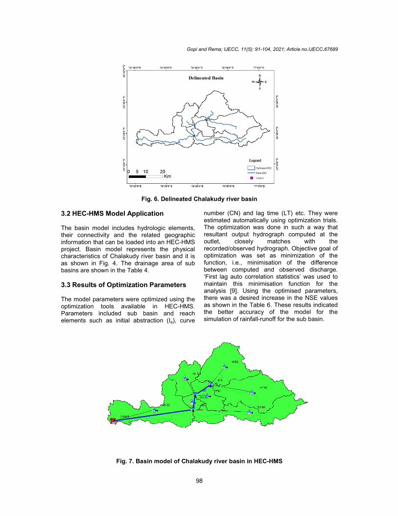
3.2 HEC-HMS Model Application The basin model includes hydrologic elements, their connectivity and the related geographic information that can be loaded into an HEC-HMS project. Basin model represents the physical characteristics of Chalakudy river basin and it is as shown in Fig. 4. The drainage area of sub basins are shown in the Table 4.

3.3 Results of Optimization Parameters The model parameters were optimized using the optimization tools available in HEC-HMS. Parameters included sub basin and reach elements such as initial abstraction (Ia), curve

number (CN) and lag time (LT) etc. They were estimated automatically using optimization trials. The optimization was done in such a way that resultant output hydrograph computed at the outlet, closely matches with the recorded/observed hydrograph. Objective goal of optimization was set as minimization of the function, i.e., minimisation of the difference between computed and observed discharge. ‘First lag auto correlation statistics’ was used to maintain this minimisation function for the analysis [9]. Using the optimised parameters, there was a desired increase in the NSE values as shown in the Table 6. These results indicated the better accuracy of the model for the simulation of rainfall-runoff for the sub basin.

Fig. 7. Basin model of Chalakudy river basin in HEC-HMS


99

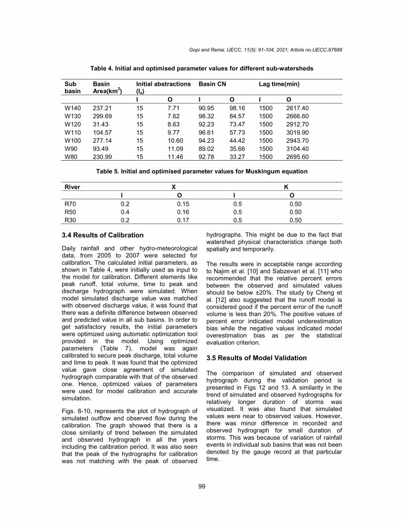
Table 4. Initial and optimised parameter values for different sub-watersheds

Sub basin

Basin Area(km

2)

Initial abstractions (Ia)

Basin CN Lag time(min)

I O I O I O

W140 237.21 15 7.71 90.95 98.16 1500 2617.40

W130 299.69 15 7.62 98.32 84.57 1500 2666.60

W120 31.43 15 8.63 92.23 73.47 1500 2912.70

W110 104.57 15 9.77 96.61 57.73 1500 3019.90

W100 277.14 15 10.60 94.23 44.42 1500 2943.70

W90 93.49 15 11.09 89.02 35.66 1500 3104.40

W80 230.99 15 11.46 92.78 33.27 1500 2695.60

Table 5. Initial and optimised parameter values for Muskingum equation

River X K

I O I O

R70 0.2 0.15 0.5 0.50

R50 0.4 0.16 0.5 0.50

R30 0.2 0.17 0.5 0.50

3.4 Results of Calibration

Daily rainfall and other hydro-meteorological data, from 2005 to 2007 were selected for calibration. The calculated initial parameters, as shown in Table 4, were initially used as input to the model for calibration. Different elements like peak runoff, total volume, time to peak and discharge hydrograph were simulated. When model simulated discharge value was matched with observed discharge value, it was found that there was a definite difference between observed and predicted value in all sub basins. In order to get satisfactory results, the initial parameters were optimized using automatic optimization tool provided in the model. Using optimized parameters (Table 7), model was again calibrated to secure peak discharge, total volume and time to peak. It was found that the optimized value gave close agreement of simulated hydrograph comparable with that of the observed one. Hence, optimized values of parameters were used for model calibration and accurate simulation.

Figs. 8-10, represents the plot of hydrograph of simulated outflow and observed flow during the calibration. The graph showed that there is a close similarity of trend between the simulated and observed hydrograph in all the years including the calibration period. It was also seen that the peak of the hydrographs for calibration was not matching with the peak of observed

hydrographs. This might be due to the fact that watershed physical characteristics change both spatially and temporarily.

The results were in acceptable range according to Najim et al. [10] and Sabzevari et al. [11] who recommended that the relative percent errors between the observed and simulated values should be below ±20%. The study by Cheng et al. [12] also suggested that the runoff model is considered good if the percent error of the runoff volume is less than 20%. The positive values of percent error indicated model underestimation bias while the negative values indicated model overestimation bias as per the statistical evaluation criterion.

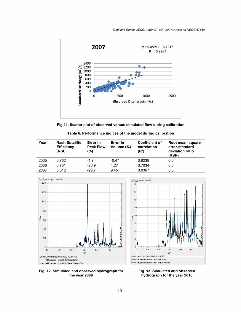
3.5 Results of Model Validation The comparison of simulated and observed hydrograph during the validation period is presented in Figs 12 and 13. A similarity in the trend of simulated and observed hydrographs for relatively longer duration of storms was visualized. It was also found that simulated values were near to observed values. However, there was minor difference in recorded and observed hydrograph for small duration of storms. This was because of variation of rainfall events in individual sub basins that was not been denoted by the gauge record at that particular time.


100

Fig. 8. Simulated and observed hydrograph for the year 2005



y = 0.7841x + 14.215R² = 0.8241

0

200

400

600

800

1000

0 500 1000Sim

ula

ted

dis

char

ge(m

3 /s)

Observed discharge(m3/s)

2005 y = 0.7323x + 12.879

R² = 0.7034

0

100

200

300

400

500

600

0 200 400 600Sim

ula

ted

Dis

char

ge(m

3 /s)

Observed Discharge(m3/s)

2006

Series1

Linear (Series1)


101

Fig.11. Scatter plot of observed versus simulated flow during calibration

Table 6. Performance indices of the model during calibration

Year Nash Sutcliffe Efficiency (NSE)

Error in Peak Flow (%)

Error in Volume (%)

Coefficient of correlation (R²)

Root mean square error-standard deviation ratio (RSR)

2005 0.762 -1.7 -0.47 0.8239 0.5

2006 0.751 -20.9 4.27 0.7034 0.5

2007 0.812 -23.7 9.45 0.8367 0.5



y = 0.8594x + 6.1247R² = 0.8367

0200400600800

100012001400

0 500 1000 1500

Sim

ula

ted

Dis

char

ge(m

3 /s)

0bserved Discharge(m3/s)

2007


102

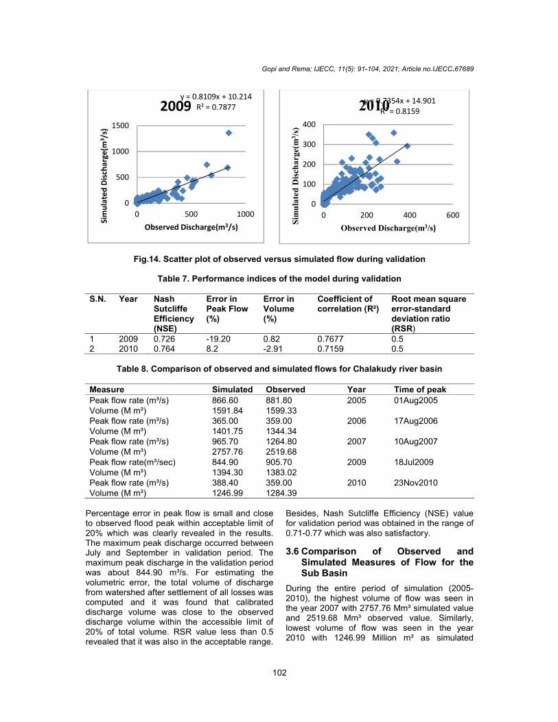
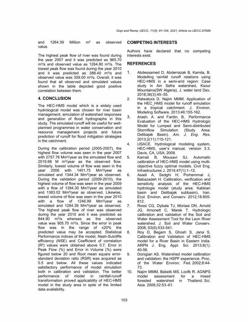
Fig.14. Scatter plot of observed versus simulated flow during validation

Table 7. Performance indices of the model during validation S.N. Year Nash

Sutcliffe Efficiency (NSE)

Error in Peak Flow (%)

Error in Volume (%)

Coefficient of correlation (R²)

Root mean square error-standard deviation ratio (RSR)

1 2009 0.726 -19.20 0.82 0.7677 0.5 2 2010 0.764 8.2 -2.91 0.7159 0.5

Table 8. Comparison of observed and simulated flows for Chalakudy river basin

Measure Simulated Observed Year Time of peak

Peak flow rate (m³/s) 866.60 881.80 2005 01Aug2005 Volume (M m³) 1591.84 1599.33 Peak flow rate (m³/s) 365.00 359.00 2006 17Aug2006 Volume (M m³) 1401.75 1344.34 Peak flow rate (m³/s) 965.70 1264.80 2007 10Aug2007 Volume (M m³) 2757.76 2519.68 Peak flow rate(m³/sec) 844.90 905.70 2009 18Jul2009 Volume (M m³) 1394.30 1383.02 Peak flow rate (m³/s) 388.40 359.00 2010 23Nov2010 Volume (M m³) 1246.99 1284.39

Percentage error in peak flow is small and close to observed flood peak within acceptable limit of 20% which was clearly revealed in the results. The maximum peak discharge occurred between July and September in validation period. The maximum peak discharge in the validation period was about 844.90 m³/s. For estimating the volumetric error, the total volume of discharge from watershed after settlement of all losses was computed and it was found that calibrated discharge volume was close to the observed discharge volume within the accessible limit of 20% of total volume. RSR value less than 0.5 revealed that it was also in the acceptable range.

Besides, Nash Sutcliffe Efficiency (NSE) value for validation period was obtained in the range of 0.71-0.77 which was also satisfactory.

3.6 Comparison of Observed and Simulated Measures of Flow for the Sub Basin

During the entire period of simulation (2005-2010), the highest volume of flow was seen in the year 2007 with 2757.76 Mm³ simulated value and 2519.68 Mm³ observed value. Similarly, lowest volume of flow was seen in the year 2010 with 1246.99 Million m³ as simulated

y = 0.8109x + 10.214R² = 0.7877

0

500

1000

1500

0 500 1000

Sim

ula

ted

Dis

char

ge(m

3 /s)


2009 y = 0.7354x + 14.901R² = 0.8159

0

100

200

300

400

0 200 400 600

Sim

ula

ted

Dis

char

ge(m

3 /s)


2010


103

and 1284.39 Million m³ as observed value. The highest peak flow of river was found during the year 2007 and it was predicted as 965.70 m³/s and observed value as 1264.80 m³/s. The lowest peak flow was found during the year 2010 and it was predicted as 388.40 m³/s and observed value was 359.00 m³/s. Overall, it was found that all observed and simulated values shown in the table depicted good positive correlation between them.

4. CONCLUSION

The HEC-HMS model which is a widely used hydrological model was chosen for river basin management, simulation of watershed responses and generation of flood hydrographs in this study. The simulated runoff will be useful for well-planned programmes in water conservation and resource management projects and future prediction of runoff for flood mitigation strategies in the catchment.

During the calibration period (2005-2007), the highest flow volume was seen in the year 2007 with 2757.76 Mm³/year as the simulated flow and 2519.68 M m³/year as the observed flow. Similarly, lowest volume of flow was seen in the year 2006 with 1401.75 Mm³/year as simulated and 1344.34 Mm³/year as observed. During the validation period (2009-2010), the highest volume of flow was seen in the year 2009 with a flow of 1394.30 Mm³/year as simulated and 1383.02 Mm³/year as observed. Likewise, lowest volume of flow was seen in the year 2010 with a flow of 1246.99 Mm³/year as simulated and 1284.39 Mm³/year as observed. The highest peak flow of river was observed during the year 2010 and it was predicted as 844.90 m³/s whereas as the observed value was 905.70 m³/s. Since the error in peak flow was in the range of ±20% the predicted value may be accepted. Statistical Performance indices of the model, Nash-Sutcliffe efficiency (NSE) and Coefficient of correlation (R²) values were obtained above 0.7, Error in Peak Flow (%) and Error in Volume (%) were figured below 20 and Root mean square error-standard deviation ratio (RSR) was acquired as 0.5 and below. All these values indicated satisfactory performance of model simulation both in calibration and validation. The better performance of model in rainfall-runoff transformation proved applicability of HEC-HMS model in the study area in spite of the limited data availability.

COMPETING INTERESTS

Authors have declared that no competing interests exist.

REFERENCES

1. Abdessamed D, Abderrazak B, Kamila, B. Modelling rainfall runoff relations using HEC-HMS in a semi-arid region: Case study in Ain Sefra watershed, Ksour Mountains(SW Algeria). J. water land Dev. 2018;36(3):45–55.

2. Halwatura D, Najim MMM. Application of the HEC_HMS model for runoff simulation in a tropical catchment. J. Environ. Modeling Software. 2013;46:155-162.

3. Arash, A. and Fardin, B.. Performance Evaluation of the HEC-HMS Hydrologic Model for Lumped and Semi-distributed Stormflow Simulation (Study Area: Delibajak Basin). Am. J. Eng. Res.

2013;2(11):115-121. 4. USACE. Hydrological modeling system,

HEC-HMS, user’s manual, version 3.3. Davis, CA, USA; 2008.

5. Kamali B, Mousavi SJ. Automatic calibration of HEC-HMS model using multi-objective fuzzy optimal models. Civil Eng. Infrastructures J. 2014;47(1):1–12.

6. Asadi A, Sedghi H, Porhemmat J, Babazadeh H. Calibration, verification and sensitivity analysis of the HEC-HMS hydrologie model (study area: Kabkian basin and Delibajak subbasin), Iran. Ecol. Environ. and Conserv. 2012;18:805-812.

7. Rossi CG, Dybala TJ, Moriasi DN, Arnold JG, Amonett C, Marek T. Hydrologic calibration and validation of the Soil and Water Assessment Tool for the Leon River watershed. J. Soil and Water Conserv. 2008; 63(6):533-541.

8. Roy D, Begam S, Ghosh S, Jana S. Calibration and Validation of HEC-HMS model for a River Basin in Eastern India. ARPN J. Eng. Appl. Sci. 2013;8(1): 40-56.

9. Donigian AS. Watershed model calibration and validation: the HSPF experience. Proc. of the Water Environ. Fed. 2002;8:44- 73.

10. Najim MMM, Babelb MS, Loofb R. AGNPS model assessment for a mixed forested watershed in Thailand. Sci. Asia. 2006;32:53–61.


104

11. Sabzevari T, Ardakanian R, Shamsaee A, Talebi A. Estimation of flood hydrograph in no statistical watersheds using HEC-HMS model and GIS (Case study: Kasilian watershed). J. Water Eng. 2009;4:1–11.

12. Cheng CT, Ou C, Chau K. Combining a fuzzy optimal model with a genetic algorithm to solve multi-objective rainfall–runoff model calibration. J. Hydrol. 2002;268:72–86.

_________________________________________________________________________________ © 2021 Gopi and Rema; This is an Open Access article distributed under the terms of the Creative Commons Attribution License (http://creativecommons.org/licenses/by/4.0), which permits unrestricted use, distribution, and reproduction in any medium, provided the original work is properly cited.

Peer-review history:

The peer review history for this paper can be accessed here: https://www.sdiarticle4.com/review-history/67689

Documents

Calibration and Validation of HEC-HMS Model for Chalakudy