Calibrating RSSI Measurements for 802.15.4 Radioshinrg.cs.jhu.edu/joomla/uploads/Main/calibrateTR.pdf · curves exhibiting the nonlinearities mentioned previously. Section 4 details

Calibrating RSSI Measurements for802.15.4 RadiosYin Chen Andreas Terzis

[email protected] [email protected]

Abstract

Wireless sensor network protocols and applications, including thoseused for localization, topology control, link scheduling, and link qual-ity estimation, make extensive use of Received Signal Strength Indi-cation (RSSI) measurements. In this paper we show that inaccuraciesin the RSSI values reported by widely used 802.15.4 radios, such asthe CC2420 and the AT86RF230, have profound impact on these pro-tocols and applications. Furthermore, we experimentally derive theresponse curves which translate actual RSSI values to the raw RSSIreadings that the radios report and show that they contain non-linearand even non-injective regions. Fortunately, these curves are consis-tent across radios of the same model, making RSSI calibration prac-tical. We present a calibration mechanism that removes the artifactsin the raw RSSI measurements, including ambiguities created by thenon-injective regions in the response curves, and generates calibratedRSSI readings that are linear. This calibration removes many of theoutliers generated when raw RSSI readings are used to estimate Signalto Noise (and Interference) ratios, estimate radio model parameters,and perform RF-based localization.

1 Introduction

The IEEE 802.15.4 standard specifies that a radio’s PHY layer must pro-vide an 8-bit integer value as an estimate of the received signal power [9].This value is commonly known as the Received Signal Strength Indication(RSSI) in the wireless sensor networks (WSN) community. Numerous WSNprotocols use RSSI measurements extensively, including those for localiza-tion [8, 12, 22, 24], link quality estimation [13, 19], packet reception ratiomodeling [23] and transmission power control [11, 17, 18].

While many protocols directly use the RSSI measurements that the ra-dios provide, the standard only requires that the reported RSSI values should

HiNRG Technical Report 1 2009-10-29

be linear and within ±6 dB of the actual RSSI values. However, ±6 dB isa wide error margin. For example, Packet Reception Ratio (PRR) can de-crease from 100% to 0% with a 2 or 3 dB difference in the received signalstrength [13]. The consequence of this observation is that possible inaccu-racies in the reported RSSI values can profoundly impact applications thatrely on RSSI measurements.

In this paper we examine two 802.15.4 compliant radios, the widely usedChipcon/TI CC2420 [20] and Atmel AT86RF230 [2], and show that they doindeed introduce systematic errors in the RSSI measurements they provide.As a matter of fact, the coarse RSSI value vs. input power graph included inthe CC2420 datasheet hints at the existence of non-linearities. Nevertheless,the manufacturer states that the RSSI response curve is very linear [20]. Weindependently derive high resolution RSSI response curves using a variablesignal generator and verify the existence of the non-linearities hinted by theCC2420 datasheet. We also note that the AT86RF230 datasheet does notprovide an equivalent graph. Fortunately, these response curves are radio-specific but device independent. In other words, different physical devicesthat use the same model of radio have identical response curves. Conse-quently, mitigating these nonlinearities does not require calibrating each de-vice individually.

This result allows us to develop a generic calibration scheme to compen-sate for the radio’s inaccuracies. Specifically, we derive a reference RSSIresponse curve which determines the calibrated RSSI value for the raw RSSIvalue that the radio reports. However, due to the existence of the non-injective regions in which a raw RSSI value maps to multiple actual RSSI val-ues, the reference RSSI response curve is not able to always provide the nec-essary mapping. To resolve this problem, we leverage the ability of 802.15.4radios to transmit at multiple power levels and dynamically fit a receiver’sraw RSSI measurements to the radio’s RSSI response curve. This approachprovides an excellent fit and is able to accurately resolve the ambiguities thatnon-injective regions generate. Finally, we present the profound impact ofthe RSSI nonlinearities and quantify the benefits of the proposed calibrationscheme on a wide variety of applications.

The paper has five additional sections. The section that follows reviewsbackground material on low-power radios and RSSI measurements. Sec-tion 3 presents the results of an experiment that investigates the influenceof packet size on the Packet Reception Ratio (PRR). Section 3 also presentsthe mechanism we developed to derive the high resolution RSSI response


curves exhibiting the nonlinearities mentioned previously. Section 4 detailsthe proposed RSSI calibration scheme, while Section 5 presents the adverseimpact of the RSSI nonlinearities on various protocols and applications, andthe improvements that the proposed calibration scheme achieves. We closein Section 6 with a brief discussion.

2 Background

Many of the popular hardware platforms in wireless sensor networks todayuse radios complying to the IEEE 802.15.4 standard [9]. This standard wasdeveloped specifically for low-power and low-cost embedded devices and im-plementations from multiple vendors are available today.

One such implementation, the TI/Chipcon CC2420 [20] is used in multi-ple platforms [5, 15]. It allows the user to select one of eight output powerlevels, ranging from -25 dBm to 0 dBm. The Atmel AT86RF230 [2] is an-other 802.15.4 radio, used in the Iris mote [6]. In addition to higher receiversensitivity this radio transmits at one of 16 power levels, from -17.2 dBm to3 dBm.

Both radios provide an 8-bit register which indicates the strength of thereceived radio signal (RSSI). The 8-bit RSSI value is averaged over 8 radiosymbol periods, i.e., 128 µs. Reported RSSI values are measured in dBm,in one dBm increments. There are two categories of RSSI measurements.The first category measures the strength of the radio signal correspondingto a received packet, while the second measures the power of the ambientchannel noise. Using these two RSSI values, one can compute the Signal-to-Noise ratio (SNR) for a received packet. We will refer to these two typesof RSSI values as signal RSSI and noise RSSI respectively throughoutthe rest of this paper. Furthermore, we name the RSSI values provided bythe radio chips as raw RSSI or reported RSSI interchangeably. We willshow that reported RSSI values are nonlinear with respect to actual receivedsignal power, defined as actual RSSI. The calibration scheme introducedin Section 4 can eliminate the nonlinearity and we term the resultant RSSIvalues as calibrated RSSI.

As part of our effort to improve the fidelity of the TOSSIM simulator [10],we performed an experiment, detailed in Section 3.1, to generate a model forthe relationship between Packet Reception Ratio (PRR) and SNR. Specifi-cally, TOSSIM does not consider the packet’s size when determining whether


5 6 7 8 90

0.2

0.4

0.6

0.8

1

SNR (dB)

Pac

ket R

ecep

tion

Rat

io

20 bytes40 bytes60 bytes80 bytes100 bytes

(a) Mote 1.

4 5 6 70

0.2

0.4

0.6

0.8

1

SNR (dB)

Pac

ket R

ecep

tion

Rat

io


(b) Mote 2.

2 3 4 5 60

0.2

0.4

0.6

0.8

1

SNR (dB)

Pac

ket R

ecep

tion

Rat

io


(c) Mote 3.

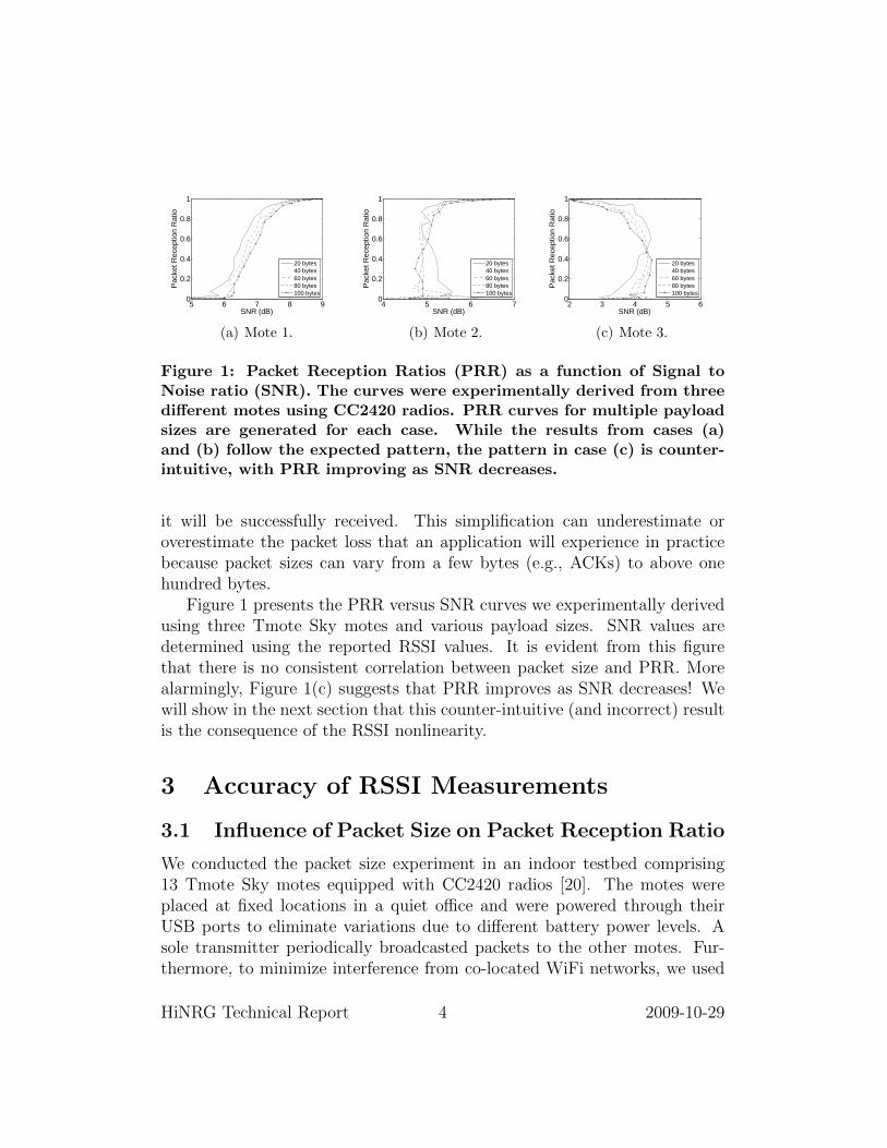
Figure 1: Packet Reception Ratios (PRR) as a function of Signal toNoise ratio (SNR). The curves were experimentally derived from threedifferent motes using CC2420 radios. PRR curves for multiple payloadsizes are generated for each case. While the results from cases (a)and (b) follow the expected pattern, the pattern in case (c) is counter-intuitive, with PRR improving as SNR decreases.

it will be successfully received. This simplification can underestimate oroverestimate the packet loss that an application will experience in practicebecause packet sizes can vary from a few bytes (e.g., ACKs) to above onehundred bytes.

Figure 1 presents the PRR versus SNR curves we experimentally derivedusing three Tmote Sky motes and various payload sizes. SNR values aredetermined using the reported RSSI values. It is evident from this figurethat there is no consistent correlation between packet size and PRR. Morealarmingly, Figure 1(c) suggests that PRR improves as SNR decreases! Wewill show in the next section that this counter-intuitive (and incorrect) resultis the consequence of the RSSI nonlinearity.

3 Accuracy of RSSI Measurements

3.1 Influence of Packet Size on Packet Reception Ratio

We conducted the packet size experiment in an indoor testbed comprising13 Tmote Sky motes equipped with CC2420 radios [20]. The motes wereplaced at fixed locations in a quiet office and were powered through theirUSB ports to eliminate variations due to different battery power levels. Asole transmitter periodically broadcasted packets to the other motes. Fur-thermore, to minimize interference from co-located WiFi networks, we used


110 120 130 140 1500

0.2

0.4

0.6

0.8

1

Batch Number

Pac

ket R

ecep

tion

Rat

io


(a) Mote 1.

110 120 130 140 1500

0.2

0.4

0.6

0.8

1

Batch Number

Pac

ket R

ecep

tion

Rat

io


(b) Mote 2.

110 120 130 140 1500

0.2

0.4

0.6

0.8

1

Batch Number

Pac

ket R

ecep

tion

Rat

io


(c) Mote 3.

Figure 2: PRR versus batch number for three motes with various pay-load sizes. All mote curves are consistent, shifted only by X-offsetscorresponding to location differences.

802.15.4 channel 26 that does not overlap with any 802.11 b/g channels [14].Considering that the mote locations are fixed and radios can transmit at

only eight power levels1, we generate a wide range of SNR values by varyingthe ambient noise level N . We do so by generating noise signals of variablepower levels using a Universal Software Radio Peripheral (USRP) [7]. Thenoise signal the USRP generates has an almost flat power spectral densitywithin the frequency range of 802.15.4 channel 26.

In this experiment, we increase the noise strength linearly (in dBm) usinga constant step size. The linearity was validated using the Anritsu MS2721Bspectrum analyzer [1]. At each noise strength level, the transmitter broad-casts a batch of 2,500 packets of five different payload sizes. To minimize theimpact of temporal variations in the radio channel, the transmitter broad-casts packets with different sizes at an inter-packet interval of 25 ms. Foreach batch of received packets we calculate the PRR and average SNR usingreported RSSI at each receiver mote. Figure 1 presents the results of thesecalculations for three receiver motes. It is clear from the mote-specific pat-terns that different motes report different results. The results in Figure 1(c)are especially puzzling, suggesting that hardware variations or even faultsmay be at play.

We use Figure 2, which plots the PRR versus batch number curves gen-erated from the same data, to verify that the radios function correctly. Notethat noise strength increases with each successive batch, while the signal

1While the CC2420 datasheet mentions a total of 31 possible transmission levels, itspecifies the output power levels for only eight of them.


strength remains constant. The SNR therefore decays as batch number in-creases and thus one expects that PRR will decrease accordingly. Indeed,Figure 2 confirms this trend. Furthermore, unlike Figure 1, the results fromthe three motes are consistent. The X-axis offsets are due to the differentlocations of the motes, leading to different received signal strengths and noiselevels. This result indicates that the underlying cause of the discrepanciesshown in Figure 1 is not device variability or failure. Instead we posit thatthey are due to inaccuracies in the RSSI values that the motes report, leadingto inaccurate SNR calculations.

3.2 RSSI Response Curves

Next, we design an experiment to derive high resolution RSSI response curvesand verify the hypothesis in the previous section that the inaccurate reportedRSSI values lead to the results presented in Figure 1.

We conducted this experiment in the same indoor testbed used for theprevious experiment. However, unlike the previous experiment, there is nomote transmitter. Instead, twelve Tmote Sky motes periodically sense thenoise signal that the USRP generates. The benefit of this approach is thatit allows us to generate signals with a much wider range of transmit powers,compared to the eight levels available from the CC2420. Like the previousexperiment, the strength of the USRP noise increases linearly (in dBm) witheach successive batch, therefore the actual RSSI at the motes should also belinear with respect to batch number. We note that although the radios reportinteger RSSI values, sub-dBm accuracy can be achieved by averaging a seriesof RSSI measurements. We also note that the noise strength increment perbatch is different from the previous experiment.

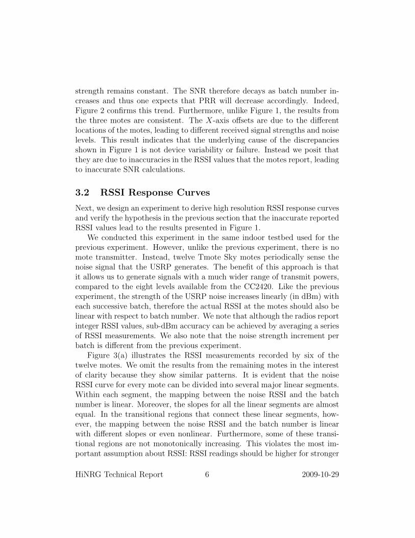
Figure 3(a) illustrates the RSSI measurements recorded by six of thetwelve motes. We omit the results from the remaining motes in the interestof clarity because they show similar patterns. It is evident that the noiseRSSI curve for every mote can be divided into several major linear segments.Within each segment, the mapping between the noise RSSI and the batchnumber is linear. Moreover, the slopes for all the linear segments are almostequal. In the transitional regions that connect these linear segments, how-ever, the mapping between the noise RSSI and the batch number is linearwith different slopes or even nonlinear. Furthermore, some of these transi-tional regions are not monotonically increasing. This violates the most im-portant assumption about RSSI: RSSI readings should be higher for stronger


0 50 100 150 200−100

−90

−80

−70

−60

−50

−40

−30

−20

−10

Batch Number

Nois

e R

SS

I (d

Bm

)

Mote 5Mote 1Mote 8

Mote 11Mote 9Mote 7

A

B

(a) 6 motes, unaligned.

0 50 100 150 200−100

−90

−80

−70

−60

−50

−40

−30

−20

−10

Batch Number

Nois

e R

SS

I (d

Bm

)

Mote 1Mote 2Mote 3Mote 4



A

B

(b) 12 motes, aligned.

Figure 3: (a) RSSI measurements reported by six Tmote Sky motesas the noise strength increases linearly in dBm. While the responseis mostly linear, it includes multiple nonlinear regions. Similar re-sults from six additional motes are omitted in the interest of clarity.(b) Aligned RSSI response curves for all twelve Tmote Sky motes.Device-specific variations are minimal. Boxes A and B indicate thenon-injective regions.

signals. In fact, this assumption is the basis of range-free localization mech-anisms [8]. Also, due to the existence of these non-monotonic regions, themapping from actual signal strength to the RSSI readings that the radiosreport is non-injective. Considering that the nonlinearities exist for all themotes tested, we categorize them as systematic errors in the RSSI measure-ments by the CC2420 radio.

Another important observation from Figure 3(a) is that the mote-specificRSSI curves are considerably similar. In fact, the major difference amongthe curves is the offset on the X-axis. This is mainly due to the differentsignal strength attenuations resulting from the varying distances betweenindividual motes and the USRP. Given this similarity, we select one RSSIcurve as the reference and align the other curves to it. Figure 3(b) showsthe result of this process. It is clear that overall the RSSI curves for differentmotes match very well. The mismatches at the lower end of the graph arelikely due to the fact that RSSI readings in this region are approaching theambient noise level.

We note that the results in Figure 3(b) were achieved by shifting theRSSI curves only along the X-axis. This is desirable because it suggests


0 50 100 150 200−100

−90

−80

−70

−60

−50

−40

−30

−20

Batch Number

Noi

se R

SS

I (dB

m)

MICAz Mote 1MICAz Mote 2

(a) MICAz motes.

0 50 100 150 200−100

−90

−80

−70

−60

−50

−40

−30

−20

Batch Number

Noi

se R

SS

I (dB

m)

Iris Mote 1Iris Mote 2Iris Mote 3

(b) IRIS motes.

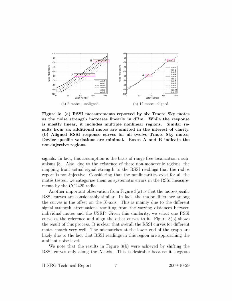
Figure 4: (a) RSSI response curves from two MICAz motes using thesame CC2420 radio as the Tmote Sky. Response curves are consistentacross platforms that use the same radio. (b) RSSI response curves forthree IRIS motes using the AT86RF230 radio. While the radio respondsdifferently from the CC2420 radio, it also has nonlinear regions.

that even though nonlinear and non-injective regions exist, they occur at thesame reported RSSI values for different motes. In other words, the device-specific variations regarding the nonlinearity and non-injectiveness are mini-mal. Consequently, mitigating these errors does not require calibrating eachdevice individually.

3.3 Platform and Radio Variability

In order to investigate the influence of the hardware platform on RSSI mea-surements, we performed the same experiment using two MICAz motes. MI-CAz motes use the same CC2420 radio but are otherwise different from theTmote Sky motes used thus far. Figure 4(a) presents the RSSI responsecurves for two MICAz motes. It is clear that the curves in Figure 4(a) arevery similar to the ones in Figure 3. This similarity indicates that the RSSImeasurement errors are caused by the CC2420 radio chip itself and are plat-form independent.

Finally, to investigate whether the observed nonlinearities are specific tothe CC2420 radio, we performed the same experiment using three CrossbowIris motes which use the AT86RF230 radio. Figure 4(b) presents the resultsfrom this experiment. While different from those in Figures 3 and 4(a), the


20 40 60 80 100 120 140 160 180 200−100

−90

−80

−70

−60

−50

−40

−30

−20

−10

Batch Number

Raw

RS

SI (

dBm

)

(a)

−80 −70 −60 −50 −40 −30 −20−100

−90

−80

−70

−60

−50

−40

−30

−20

−10

Calibrated RSSI (dBm)

Raw

RS

SI (

dBm

)

Reference Curve

(b)

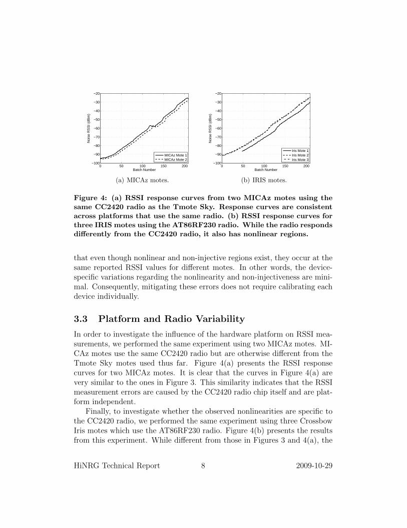
Figure 5: (a) Combination of the 12 curves in Figure 3(b). (b) The ref-erence RSSI curve for CC2420 radios, derived by linearly transformingthe X-axis from (a).

RSSI response graphs of the IRIS motes exhibit consistent nonlinearities.On the other hand, the RSSI response graphs do not exhibit non-injectiveregions. Finally, we observe consistent non-linearities across all three motes,indicating that the systematic errors in AT86RF230 raw RSSI measurementsare also device independent.

4 RSSI Calibration

The results from the previous section show that radios have a non-linear,yet consistent response curve that maps the actual received signal strengthto reported RSSI measurements. Figure 5(a), derived from combining theindividual curves in Figure 3(b), shows such a response curve for the CC2420radio. The issue with this curve is that the X-axis is in units of batch numberinstead of actual RSSI values. The noise strength increases linearly withrespect to the batch number and therefore the relationship between batchnumber (n) and actual RSSI (r) should be r = α×n+β. The noise strengthincrement α can be measured experimentally, using the Anritsu MS2721B.On the other hand, measuring β accurately would require measuring thepower of the signal that comes out of the receiving mote’s antenna with apre-calibrated receiver. Fortunately, as we explain next, we do not need toestimate β accurately.


−80 −70 −60 −50 −40 −30 −20−100

−90

−80

−70

−60

−50

−40

−30

−20

−10


Raw

RS

SI (d

Bm

)

Reference Curve

Receiver 1Receiver 2

Receiver 3

(a)

−80 −70 −60 −50 −40 −30 −20−100

−90

−80

−70

−60

−50

−40

−30

−20

−10


Raw

RS

SI (

dBm

)

Reference CurveReceiver 1Receiver 2Receiver 3

(b)

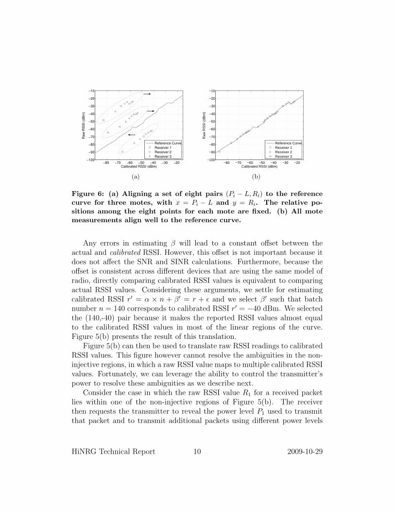
Figure 6: (a) Aligning a set of eight pairs (Pi − L,Ri) to the referencecurve for three motes, with x = Pi − L and y = Ri. The relative po-sitions among the eight points for each mote are fixed. (b) All motemeasurements align well to the reference curve.

Any errors in estimating β will lead to a constant offset between theactual and calibrated RSSI. However, this offset is not important because itdoes not affect the SNR and SINR calculations. Furthermore, because theoffset is consistent across different devices that are using the same model ofradio, directly comparing calibrated RSSI values is equivalent to comparingactual RSSI values. Considering these arguments, we settle for estimatingcalibrated RSSI r′ = α × n + β′ = r + ε and we select β′ such that batchnumber n = 140 corresponds to calibrated RSSI r′ = −40 dBm. We selectedthe (140,-40) pair because it makes the reported RSSI values almost equalto the calibrated RSSI values in most of the linear regions of the curve.Figure 5(b) presents the result of this translation.

Figure 5(b) can then be used to translate raw RSSI readings to calibratedRSSI values. This figure however cannot resolve the ambiguities in the non-injective regions, in which a raw RSSI value maps to multiple calibrated RSSIvalues. Fortunately, we can leverage the ability to control the transmitter’spower to resolve these ambiguities as we describe next.

Consider the case in which the raw RSSI value R1 for a received packetlies within one of the non-injective regions of Figure 5(b). The receiverthen requests the transmitter to reveal the power level P1 used to transmitthat packet and to transmit additional packets using different power levels


P2, . . . , Pm2. The receiver records the raw RSSI values R2, . . . , Rm for each

of the additional packets. If at least one of the Ri’s falls within the radio’sinjective response region, it is possible to translate it to the calibrated RSSIvalue R′

i via Figure 5(b). Note that R′i = Pi − L, where L is the link at-

tenuation in dB. Knowing the values for both Pi and R′i we can solve for L.

Then P1 − L can be assigned to be the calibrated RSSI value correspondingto R1, because L is consistent across different transmit powers. The com-putational cost is trivial, because only one raw RSSI value (Ri) needs to betranslated into the calibrated RSSI (R′

i), via a lookup table corresponding tothe reference curve.

To be more robust against measurement errors and noise, we can alsoselect the value of L that minimizes the mean square difference betweenthe m points (P1 − L,R1), . . . , (Pm − L,Rm) and the reference curve. Thecomputational cost would be increased in this case because multiple tablelookups are necessary.

Figures 6(a) and 6(b) present an example of the m-point calibration pro-cess for three receivers, with m = 8, equal to the number of power levelsavailable in CC2420. One can see that the eight points for each mote fitwell to the reference curve. Note that generally m can be arbitrarily chosenbetween 2 and the number of available power levels.

5 Applications

In what follows we explore the impact of RSSI calibration in modeling, pro-tocol behavior, application performance, and simulation veracity.

5.1 PRR-SNR Model

First, we investigate the benefits of applying the RSSI calibration mecha-nism described in Section 4 to the problem of understanding the relationshipbetween PRR and SNR. In turn, this understanding can be used in a vari-ety of applications ranging from online link estimation to link modeling andsimulation.

We conducted this experiment in the same indoor testbed used for thepacket size experiment. One Tmote Sky mote was chosen as the transmitter

2The number m is upper-bounded by the number of available transmit power levelsfrom the radio, and the actual Pi values are listed on the radio’s datasheet.


while the other twelve motes acted as receivers. However, unlike the packetsize experiment, all packets had the same size. Moreover, the transmittervaried the output power levels to produce a larger range of SNR values.

The signal to noise ratio (SNR) is computed as SNR = SN

, where S isthe power of the received packet and N is the power of the ambient noise.Let both S and N be measured in milliwatts (mW). In logarithmic scalethe above equation becomes SNRdB = SdBm−NdBm where SdBm and NdBm

are the logarithmic scale powers of the received signal and ambient noiserespectively.

In order to measure S and N , the receivers record both packet RSSI(SRSSI) and noise RSSI (NRSSI). Then, SRSSI = 10 log10(S + N) andNRSSI = 10 log10N . Therefore, SRSSI is essentially the sum of the powerof the radio signal and the power of the noise. Nevertheless, when SRSSI �NRSSI one can approximate SNR as SNRdB ≈ SRSSI −NRSSI . On the otherhand, when SRSSI is comparable to NRSSI we need to compute SNR through

SNRdB = 10 log10(10SRSSI/10 − 10NRSSI/10)−NRSSI (1)

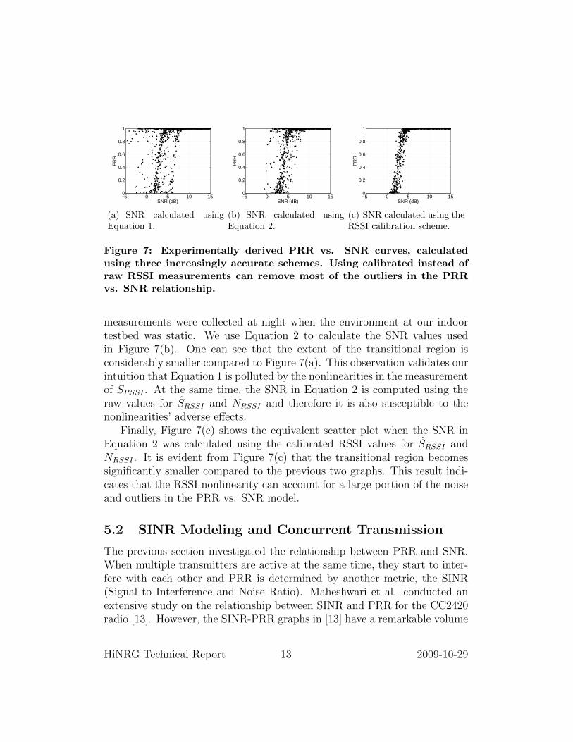
because S = 10SRSSI/10 − 10NRSSI/10.We use Equation 1 to calculate the SNR values used in the PRR vs. SNR

scatter plot shown in Figure 7(a). One can see from this figure that there isa large transitional region, through which the relationship between PRR andSNR is noisy and unpredictable. The existence of this transitional region hasbeen widely reported in the wireless sensor networks literature [21, 23, 25].

At the same time, given the nonlinearity presented in Figure 3(b), usingraw RSSI values to calculate SNR can be problematic. For instance, if Sand N are both within the non-injective regions, the reported RSSI value fortheir sum might be smaller than the reported RSSI value for S or N alone.

To eliminate this issue, we configured the transmitter to broadcast oneadditional batch of packets at each of the eight output power levels, whilekeeping the USRP turned off. This allows us to use the packet RSSI mea-surements directly, without having to calculate S from SRSSI and NRSSI . Inthis case, we denote the reported packet RSSI value as SRSSI , and calculateSNR as

SNRdB = SRSSI −NRSSI (2)

Doing so assumes that the channel conditions do not change dramaticallythroughout the course of the experiment. This is however reasonable, as the


−5 0 5 10 150

0.2

0.4

0.6

0.8

1

SNR (dB)

PR

R

(a) SNR calculated usingEquation 1.

−5 0 5 10 150

0.2

0.4

0.6

0.8

1

SNR (dB)

PR

R

(b) SNR calculated usingEquation 2.

−5 0 5 10 150

0.2

0.4

0.6

0.8

1

SNR (dB)

PR

R

(c) SNR calculated using theRSSI calibration scheme.

Figure 7: Experimentally derived PRR vs. SNR curves, calculatedusing three increasingly accurate schemes. Using calibrated instead ofraw RSSI measurements can remove most of the outliers in the PRRvs. SNR relationship.

measurements were collected at night when the environment at our indoortestbed was static. We use Equation 2 to calculate the SNR values usedin Figure 7(b). One can see that the extent of the transitional region isconsiderably smaller compared to Figure 7(a). This observation validates ourintuition that Equation 1 is polluted by the nonlinearities in the measurementof SRSSI . At the same time, the SNR in Equation 2 is computed using theraw values for SRSSI and NRSSI and therefore it is also susceptible to thenonlinearities’ adverse effects.

Finally, Figure 7(c) shows the equivalent scatter plot when the SNR inEquation 2 was calculated using the calibrated RSSI values for SRSSI andNRSSI . It is evident from Figure 7(c) that the transitional region becomessignificantly smaller compared to the previous two graphs. This result indi-cates that the RSSI nonlinearity can account for a large portion of the noiseand outliers in the PRR vs. SNR model.

5.2 SINR Modeling and Concurrent Transmission

The previous section investigated the relationship between PRR and SNR.When multiple transmitters are active at the same time, they start to inter-fere with each other and PRR is determined by another metric, the SINR(Signal to Interference and Noise Ratio). Maheshwari et al. conducted anextensive study on the relationship between SINR and PRR for the CC2420radio [13]. However, the SINR-PRR graphs in [13] have a remarkable volume


−10 −8 −6 −4 −2 0 2 4 6 8 100

0.1

0.2

0.3

0.4

0.5

0.6

0.7

0.8

0.9

1

SINR (dB)

PR

RA

B

(a) Raw SINR.

−10 −8 −6 −4 −2 0 2 4 6 8 100

0.1

0.2

0.3

0.4

0.5

0.6

0.7

0.8

0.9

1

SINR (dB)

PR

R

(b) Calibrated SINR.

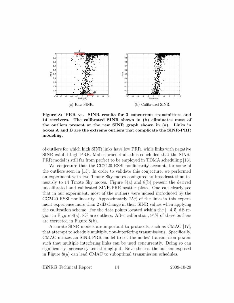
Figure 8: PRR vs. SINR results for 2 concurrent transmitters and14 receivers. The calibrated SINR shown in (b) eliminates most ofthe outliers present at the raw SINR graph shown in (a). Links inboxes A and B are the extreme outliers that complicate the SINR-PRRmodeling.

of outliers for which high SINR links have low PRR, while links with negativeSINR exhibit high PRR. Maheshwari et al. thus concluded that the SINR-PRR model is still far from perfect to be employed in TDMA scheduling [13].

We conjecture that the CC2420 RSSI nonlinearity accounts for some ofthe outliers seen in [13]. In order to validate this conjecture, we performedan experiment with two Tmote Sky motes configured to broadcast simulta-neously to 14 Tmote Sky motes. Figure 8(a) and 8(b) present the deriveduncalibrated and calibrated SINR-PRR scatter plots. One can clearly seethat in our experiment, most of the outliers were indeed introduced by theCC2420 RSSI nonlinearity. Approximately 25% of the links in this experi-ment experience more than 2 dB change in their SINR values when applyingthe calibration scheme. For the data points located within the [−4, 5] dB re-gion in Figure 8(a), 8% are outliers. After calibration, 94% of these outliersare corrected in Figure 8(b).

Accurate SINR models are important to protocols, such as CMAC [17],that attempt to schedule multiple, non-interfering transmissions. Specifically,CMAC utilizes an SINR-PRR model to set the nodes’ transmission powerssuch that multiple interfering links can be used concurrently. Doing so cansignificantly increase system throughput. Nevertheless, the outliers exposedin Figure 8(a) can lead CMAC to suboptimal transmission schedules.


0 2 4 6 8 100

0.2

0.4

0.6

0.8

1

SNR (dB)

PR

R

(a)

0 2 4 6 8 100

0.2

0.4

0.6

0.8

1

SNR (dB)

PR

R

−58−90−72−53

(b)

0 2 4 6 8 100

0.2

0.4

0.6

0.8

1

SNR (dB)

PR

R

−65−63

(c)

Figure 9: PRR vs. SNR curves generated by a TOSSIM simulation. (a)shows the curve from the original TOSSIM. Curves in (b) and (c) arederived from a modified version of TOSSIM that simulates the CC2420RSSI nonlinearity. Each curve in (b) and (c) was derived by keeping thenoise power constant and varying signal strength to create a dynamicSNR range. The noise power listed in the legends is in dBm units.

For example, we observed in the experiment that one of the two senders(mote 0) could deliver > 98% of its packets to receiver 11 when transmittingat -7 dBm, while the other sender (mote 1) could deliver at the same time >98% of its packets to receiver 14 using transmit power of -15 dBm. However,the raw SINR value calculated at mote 14 is -0.128 dB which translates to avery low PRR according to the SINR-PRR model. For this reason, a powerscheduling protocol based on the SINR model, such as CMAC [17], wouldnot schedule mote 1 to transmit at power -15 dBm. On the other hand, ifCMAC used the calibrated SINR value at mote 14 (= 2.2056 dB) it wouldcorrectly schedule the concurrent transmission. We note that link 1→ 14 isone of the links in box A shown in Figure 8(a).

5.3 WSN Simulation

Existing wireless sensor network simulators such as TOSSIM [10] do notsimulate the radio-specific RSSI measurement nonlinearities. Nevertheless,it is straightforward to integrate RSSI response curves, such as the one inFigure 5(b), to these simulators. Doing so requires constructing a lookuptable and using linear interpolation to convert actual RSSI values (i.e., X-axis in Figure 5(b)) into reported RSSI values (i.e., Y -axis in Figure 5(b)).

We implemented such a mechanism for TOSSIM and Figure 9 presentsa few sample PRR-SNR curves. Specifically, Figure 9(a) shows the PRR


With Nonlinearity Without Nonlinearity0%1%2%3%4%5%6%7%8%9%

Est

imat

ion

Err

or (

%)

nPr(d0)σ

(a) n = 3.5, Pr(d0) = −30, σ = 3

With Nonlinearity Without Nonlinearity0%

5%

10%

15%

20%

Est

imat

ion

Err

or (

%)

nPr(d0)σ

(b) n = 2, Pr(d0) = −30, σ = 3

Figure 10: Errors in estimating log-normal path loss model parameters.

versus reported SNR curve in the current version of TOSSIM. Without theintegration of the RSSI response curve, the shape of this PRR-SNR curvedoes not change as RSSI varies. In contrast, Figures 9(b) and 9(c) showthat different curves emerge as we vary the power of the ambient noise, dueto the nonlinearity in the reported RSSI values. In particular, the curvesin Figure 9(c) resemble the experimentally derived curves in Figures 1(b)and 1(c).

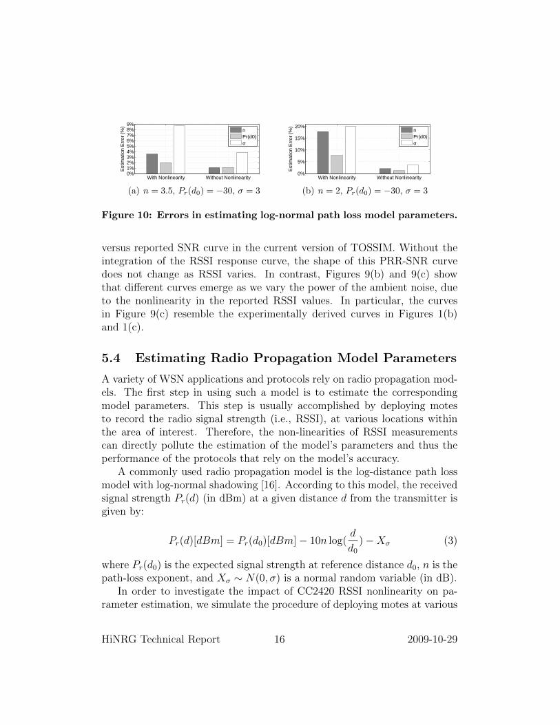
5.4 Estimating Radio Propagation Model Parameters

A variety of WSN applications and protocols rely on radio propagation mod-els. The first step in using such a model is to estimate the correspondingmodel parameters. This step is usually accomplished by deploying motesto record the radio signal strength (i.e., RSSI), at various locations withinthe area of interest. Therefore, the non-linearities of RSSI measurementscan directly pollute the estimation of the model’s parameters and thus theperformance of the protocols that rely on the model’s accuracy.

A commonly used radio propagation model is the log-distance path lossmodel with log-normal shadowing [16]. According to this model, the receivedsignal strength Pr(d) (in dBm) at a given distance d from the transmitter isgiven by:

Pr(d)[dBm] = Pr(d0)[dBm]− 10n log(d

d0)−Xσ (3)

where Pr(d0) is the expected signal strength at reference distance d0, n is thepath-loss exponent, and Xσ ∼ N(0, σ) is a normal random variable (in dB).

In order to investigate the impact of CC2420 RSSI nonlinearity on pa-rameter estimation, we simulate the procedure of deploying motes at various


distances from a transmitter to derive the log-normal parameters Pr(d0), nand σ. Specifically, we generate the Pr(d) samples using a set of log-normalparameters and use the RSSI measurements to estimate those parameters.We note that doing so assumes that the log-normal model perfectly char-acterizes the RF propagation, a premise which might be violated in reality.Nevertheless, this treatment isolates the sources of errors in model parameterestimation and therefore allow us to focus on the errors that the RSSI non-linearity introduces. A total of 240 samples were generated, corresponding tomeasurements collected at locations uniformly spaced at distances between1 and 30 meters from the transmitter. Two samples were generated for eachdistance. Figure 10 presents the estimation errors with and without the pres-ence of the CC2420 RSSI nonlinearity for two sets of model parameters. Itis clear that the nonlinearity can cause significant errors. Errors in estimat-ing these parameters can directly impact the applications that rely on them,such as RF based localization [24] and network coverage prediction [4].

5.5 RF Based Localization

Localization techniques based on RF signal strength use RSSI measurementsto estimate the distances of a mobile device to several reference servers whoselocations are known. Trilateration can then be used to estimate the device’slocation [24]. The previous section demonstrated that the nonlinearities inthe CC2420 RSSI measurements impact the estimation of the radio modelparameters. In turn, these errors can directly diminish the accuracy of suchlocalization algorithms. On the other hand, localization schemes that employRSSI signatures should intuitively be less affected by such nonlinearities.For example, the RADAR system collects a database of RSSI signatures byhaving a mobile node broadcast packets to three reference servers from aset of known locations [3]. The resulting RSSI measurements collected atthe three servers, along with the mobile device’s location, form the 5-tuples[RSSI1, RSSI2, RSSI3, X, Y ] that constitute the localization database.

Once this training phase is complete, a device that needs to estimate itslocation broadcasts a series of packets to the reference servers. The systemthen finds the entry in the localization database with the minimum meansquare difference from the RSSI measurements and uses the entry’s [X, Y ]coordinates as the estimate of the node’s current location. The MoteTracksystem extends this simple approach and makes it highly robust and decen-tralized [12].


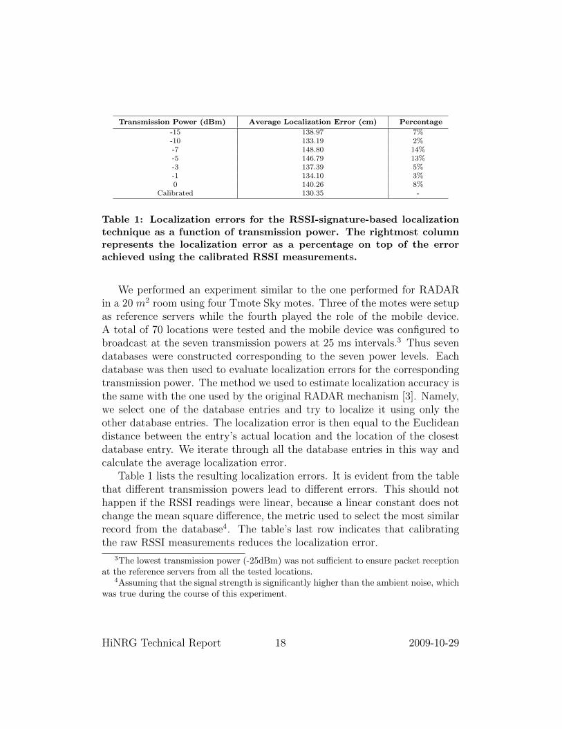
Transmission Power (dBm) Average Localization Error (cm) Percentage

-15 138.97 7%-10 133.19 2%-7 148.80 14%-5 146.79 13%-3 137.39 5%-1 134.10 3%0 140.26 8%

Calibrated 130.35 -

Table 1: Localization errors for the RSSI-signature-based localizationtechnique as a function of transmission power. The rightmost columnrepresents the localization error as a percentage on top of the errorachieved using the calibrated RSSI measurements.

We performed an experiment similar to the one performed for RADARin a 20 m2 room using four Tmote Sky motes. Three of the motes were setupas reference servers while the fourth played the role of the mobile device.A total of 70 locations were tested and the mobile device was configured tobroadcast at the seven transmission powers at 25 ms intervals.3 Thus sevendatabases were constructed corresponding to the seven power levels. Eachdatabase was then used to evaluate localization errors for the correspondingtransmission power. The method we used to estimate localization accuracy isthe same with the one used by the original RADAR mechanism [3]. Namely,we select one of the database entries and try to localize it using only theother database entries. The localization error is then equal to the Euclideandistance between the entry’s actual location and the location of the closestdatabase entry. We iterate through all the database entries in this way andcalculate the average localization error.

Table 1 lists the resulting localization errors. It is evident from the tablethat different transmission powers lead to different errors. This should nothappen if the RSSI readings were linear, because a linear constant does notchange the mean square difference, the metric used to select the most similarrecord from the database4. The table’s last row indicates that calibratingthe raw RSSI measurements reduces the localization error.

3The lowest transmission power (-25dBm) was not sufficient to ensure packet receptionat the reference servers from all the tested locations.

4Assuming that the signal strength is significantly higher than the ambient noise, whichwas true during the course of this experiment.


6 Conclusion

This paper verifies the existence of the oft-ignored RSSI non-linearities forthe popular Chipcon/TI CC2420 802.15.4 radio and shows that similar non-linearities exist in the Atmel AT86RF230 radio. Furthermore, the paperexperimentally derives the non-linear RSSI response curves for the two radios,shows that they are consistent across devices that use the same model ofradio, and proposes a scheme to calibrate raw RSSI measurements includingthose that fall within a curve’s non-injective regions. Last but not least,we evaluate the impact of non-linearities in RSSI measurements on PRRmodeling, WSN simulation, as well as protocols for concurrent link schedulingand RF-based localization.

The implications of our results to future designs are twofold. First, proto-col and application designers need to be mindful that RSSI response curvesmay be non-linear or even non-injective and include techniques to compen-sate for such non-linearities. Second, considering the dependence of multipleprotocols on RSSI measurements, future radio designs should strive to pro-duce linear or at least injective RSSI response curves.

The calibration data used in this paper is available online at http://

www.cs.jhu.edu/~yinchen/calibrate.

Acknowledgments

We extend our gratitude to Neal Patwari, Phil Levis, and Prabal Dutta fortheir insightful comments and suggestions. We would also like to thank theanonymous reviewers that for helping us improve the paper’s presentation.This research was supported in part by NSF grants CNS-0834470 and CNS-0546648. Any opinions, finding, conclusions or recommendations expressedin this publication are those of the authors and do not represent the policyor position of the NSF.

References

[1] Anritsu Company. Spectrum Master MS2721B.

[2] Atmel Corporation. AT86RF230: Low Power 2.4 GHz Transceiver for ZigBee,IEEE 802.15.4, 6LoWPAN, RF4CE and ISM applications.


http://www.cs.jhu.edu/~yinchen/calibrate

http://www.cs.jhu.edu/~yinchen/calibrate

[3] P. Bahl and V. N. Padmanabhan. RADAR: An In-Building RF-based UserLocation and Tracking System. In Proceedings of INFOCOM, 2000.

[4] O. Chipara, G. Hackmann, C. Lu, W. D. Smart, and G.-C. Roman. Radiomapping for indoor environments. Technical report, Washington Universityin St. Louis, 2007.

[5] Crossbow Corporation. MICAz Specifications, 2004.

[6] Crossbow Corporation. Iris Specifications, 2007.

[7] Ettus Research LLC. Universal Software Radio Peripheral, 2007.

[8] T. He, C. Huang, B. M. Blum, J. A. Stankovic, and T. Abdelzaher. Range-free localization schemes for large scale sensor networks. In MobiCom ’03,pages 81–95, New York, NY, USA, 2003. ACM.

[9] IEEE Standard 802.15.4: Wireless Medium Access Control (MAC) and Physi-cal Layer (PHY) Specifications for Low-Rate Wireless Personal Area Networks(LR-WPANs), May 2003.

[10] P. Levis, N. Lee, A. Woo, M. Welsh, and D. Culler. TOSSIM: Accurate andscalable simulation of entire TinyOS Applications. In Proceedings of Sensys2003, Nov. 2003.

[11] S. Lin, J. Zhang, G. Zhou, L. Gu, J. A. Stankovic, and T. He. ATPC AdaptiveTransmission Power Control for Wireless Sensor Networks. In Proceedings ofthe 4th ACM Sensys Conference, 2006.

[12] K. Lorincz and M. Welsh. Motetrack: a robust, decentralized approach to rf-based location tracking. Personal Ubiquitous Comput., 11(6):489–503, 2007.

[13] R. Maheshwari, S. Jain, and S. R. Das. A measurement study of interferencemodeling and scheduling in low-power wireless networks. In Proceedings ofSensys 2008, pages 141–154, New York, NY, USA, 2008. ACM.

[14] R. Musaloiu-E. and A. Terzis. Minimising the effect of wifi interference in802.15.4 wireless sensor networks. Int. J. Sen. Netw., 3(1):43–54, 2007.

[15] J. Polastre, R. Szewczyk, and D. Culler. Telos: Enabling Ultra-Low PowerWireless Research. In IPSN/SPOTS 05, Apr. 2005.

[16] T. S. Rappaport. Wireless Communications: Principles & Practices. PrenticeHall, 1996.


[17] M. Sha, G. Xing, G. Zhou, S. Liu, and X. Wang. C-MAC: Model-driven Con-current Medium Access Control for Wireless Sensor Networks. In Proceedingsof IEEE Infocom, 2009.

[18] D. Son, B. Krishnamachari, and J. Heidemann. Experimental study of concur-rent transmission in wireless sensor networks. In Proceedings of ACM Sensys,2006.

[19] K. Srinivasan and P. Levis. RSSI is Under Appreciated. In Proceedings of the3rd Workshop on Embedded Networked Sensors (EmNets), May 2006.

[20] Texas Instruments. CC2420: 2.4 GHz IEEE 802.15.4 / ZigBee-ready RFTransceiver, 2006.

[21] A. Woo, T. Tong, and D. Culler. Taming the underlying challenges in reliablemultihop wireless sensor networks. In Proceedings of ACM Sensys, 2003.

[22] K. Yedavalli, B. Krishnamachari, S. Ravula, and B. Srinivasan. Ecolocation:a sequence based technique for rf localization in wireless sensor networks. InProceedings of IPSN 2005, page 38, Piscataway, NJ, USA, 2005. IEEE Press.

[23] M. Z. Zamalloa and B. Krishnamachari. An analysis of unreliability and asym-metry in low-power wireless links. ACM Transactions on Sensor Networks,June 2007.

[24] G. Zanca, F. Zorzi, A. Zanella, and M. Zorzi. Experimental comparisonof rssi-based localization algorithms for indoor wireless sensor networks. InREALWSN ’08, pages 1–5, New York, NY, USA, 2008. ACM.

[25] J. Zhao and R. Govindan. Understanding Packet Delivery Performance InDense Wireless Sensor Networks. In Proceedings of the ACM Sensys, Nov.2003.


Documents

Calibrating RSSI Measurements for 802.15.4 Radioshinrg.cs.jhu.edu/joomla/uploads/Main/calibrateTR.pdf · curves exhibiting the nonlinearities mentioned previously. Section 4 details