Embed Size (px)
Citation preview

CalibratingEnvironmental
EngineeringModels
David Ruppert
Outline
BackgroundThe team
The research problem
The ModelEnvironmental model
Modeling the noise
Likelihood
MethodologyOverview
Locating mode
Experimental Design
RBF approximation
MCMC sampling
Case StudyChemical spill model
Monte Carlo
Summary
Calibrating Environmental Engineering Models
David Ruppert
Cornell University
November 4, 2006

CalibratingEnvironmental
EngineeringModels
David Ruppert
Outline
BackgroundThe team
The research problem
The ModelEnvironmental model
Modeling the noise
Likelihood
MethodologyOverview
Locating mode
Experimental Design
RBF approximation
MCMC sampling
Case StudyChemical spill model
Monte Carlo
Summary
What this talk is about
1 BackgroundThe teamThe research problem
2 The ModelEnvironmental modelModeling the noiseLikelihood
3 MethodologyOverviewLocating modeExperimental DesignRBF approximationMCMC sampling
4 Case StudyChemical spill modelMonte Carlo
5 Summary

CalibratingEnvironmental
EngineeringModels
David Ruppert
Outline
BackgroundThe team
The research problem
The ModelEnvironmental model
Modeling the noise
Likelihood
MethodologyOverview
Locating mode
Experimental Design
RBF approximation
MCMC sampling
Case StudyChemical spill model
Monte Carlo
Summary
Project Team
Christine Shoemaker, co-PI, Professor of Civil andEnvironmental Engineering
PhD in applied mathworks in applied optimization
David Ruppert, co-PINikolai Blizniouk, PhD student in Operations ResearchChristine’s students and post-docs
Rommel RegisStefan WildPradeep Mugunthan

CalibratingEnvironmental
EngineeringModels
David Ruppert
Outline
BackgroundThe team
The research problem
The ModelEnvironmental model
Modeling the noise
Likelihood
MethodologyOverview
Locating mode
Experimental Design
RBF approximation
MCMC sampling
Case StudyChemical spill model
Monte Carlo
Summary
Work of Chris Shoemaker and her students
Christine Shoemaker’s research:
global optimizationoptimization of computationally expensive functionsmethods for calibration and uncertainty analysisexample: remediation of a US-DOD site
contaminated with chlorinated ethenes in the soil andgroundwater

CalibratingEnvironmental
EngineeringModels
David Ruppert
Outline
BackgroundThe team
The research problem
The ModelEnvironmental model
Modeling the noise
Likelihood
MethodologyOverview
Locating mode
Experimental Design
RBF approximation
MCMC sampling
Case StudyChemical spill model
Monte Carlo
Summary
Calibrating Environment Models
Typical problem in environmental engineering:remediation of comtaminated groundwater
Modeled as a system of partial differential equationsdescribing
movement of pollutantschemical reactions
Coefficients are unknownCalibration means estimation of parameters in model
this is an inverse problemalso a nonlinear regression problem

CalibratingEnvironmental
EngineeringModels
David Ruppert
Outline
BackgroundThe team
The research problem
The ModelEnvironmental model
Modeling the noise
Likelihood
MethodologyOverview
Locating mode
Experimental Design
RBF approximation
MCMC sampling
Case StudyChemical spill model
Monte Carlo
Summary
Why is Calibration Difficult?
Likelihood may be multimodalNon-Gaussian dataSpatial and temporal correlationsModel is computationally expensive
May take minutes or even hours to evaluate the model forone set of parameter values

CalibratingEnvironmental
EngineeringModels
David Ruppert
Outline
BackgroundThe team
The research problem
The ModelEnvironmental model
Modeling the noise
Likelihood
MethodologyOverview
Locating mode
Experimental Design
RBF approximation
MCMC sampling
Case StudyChemical spill model
Monte Carlo
Summary
Deterministic component of model
ith observation is
Yi = (Yi,1, . . . , Yi,d)T
in absence of noise:
Yi,j = fj(Xi ,β)
fj(·) comes from scientific theoryXi is a covariate vectorβ contains the parameters of interest
noise is modeled empirically

CalibratingEnvironmental
EngineeringModels
David Ruppert
Outline
BackgroundThe team
The research problem
The ModelEnvironmental model
Modeling the noise
Likelihood
MethodologyOverview
Locating mode
Experimental Design
RBF approximation
MCMC sampling
Case StudyChemical spill model
Monte Carlo
Summary
Components of the noise model
We modeled the noise via:data transformationspatial-temporal correlation model

CalibratingEnvironmental
EngineeringModels
David Ruppert
Outline
BackgroundThe team
The research problem
The ModelEnvironmental model
Modeling the noise
Likelihood
MethodologyOverview
Locating mode
Experimental Design
RBF approximation
MCMC sampling
Case StudyChemical spill model
Monte Carlo
Summary
Purpose of data transformation
We used transformations to:normalize the response distributionstabilize the variance

CalibratingEnvironmental
EngineeringModels
David Ruppert
Outline
BackgroundThe team
The research problem
The ModelEnvironmental model
Modeling the noise
Likelihood
MethodologyOverview
Locating mode
Experimental Design
RBF approximation
MCMC sampling
Case StudyChemical spill model
Monte Carlo
Summary
Transform-both-sides model
The transform-both-sides model is
h {Yi,j , λj} = h {fj(Xi ,β), λj}+ εi,j ,
equivalently
Yi,j = h−1 [h {fj(Xi ,β), λj}+ εi,j , λj ]
transforms both sides of the equation giving deterministicmodelpreserves the theoretical model{h(·, λ) : λ ∈ Λ} is some transformation family

CalibratingEnvironmental
EngineeringModels
David Ruppert
Outline
BackgroundThe team
The research problem
The ModelEnvironmental model
Modeling the noise
Likelihood
MethodologyOverview
Locating mode
Experimental Design
RBF approximation
MCMC sampling
Case StudyChemical spill model
Monte Carlo
Summary
Transform-both-sides model
The transform-both-sides model is
h {Yi,j , λj} = h {fj(Xi ,β), λj}+ εi,j ,
equivalently
Yi,j = h−1 [h {fj(Xi ,β), λj}+ εi,j , λj ]
transforms both sides of the equation giving deterministicmodel
preserves the theoretical model{h(·, λ) : λ ∈ Λ} is some transformation family

CalibratingEnvironmental
EngineeringModels
David Ruppert
Outline
BackgroundThe team
The research problem
The ModelEnvironmental model
Modeling the noise
Likelihood
MethodologyOverview
Locating mode
Experimental Design
RBF approximation
MCMC sampling
Case StudyChemical spill model
Monte Carlo
Summary
Transform-both-sides model
The transform-both-sides model is
h {Yi,j , λj} = h {fj(Xi ,β), λj}+ εi,j ,
equivalently
Yi,j = h−1 [h {fj(Xi ,β), λj}+ εi,j , λj ]
transforms both sides of the equation giving deterministicmodelpreserves the theoretical model
{h(·, λ) : λ ∈ Λ} is some transformation family

CalibratingEnvironmental
EngineeringModels
David Ruppert
Outline
BackgroundThe team
The research problem
The ModelEnvironmental model
Modeling the noise
Likelihood
MethodologyOverview
Locating mode
Experimental Design
RBF approximation
MCMC sampling
Case StudyChemical spill model
Monte Carlo
Summary
Transform-both-sides model
The transform-both-sides model is
h {Yi,j , λj} = h {fj(Xi ,β), λj}+ εi,j ,
equivalently
Yi,j = h−1 [h {fj(Xi ,β), λj}+ εi,j , λj ]
transforms both sides of the equation giving deterministicmodelpreserves the theoretical model{h(·, λ) : λ ∈ Λ} is some transformation family

CalibratingEnvironmental
EngineeringModels
David Ruppert
Outline
BackgroundThe team
The research problem
The ModelEnvironmental model
Modeling the noise
Likelihood
MethodologyOverview
Locating mode
Experimental Design
RBF approximation
MCMC sampling
Case StudyChemical spill model
Monte Carlo
Summary
Transform-both-sides examples
the identity transformation gives the usual nonlinearregression model
additive Gaussian errorsif we use the log transformation then
Yi,j = exp [log{fj(Xi ,β)}+ εi,j ] = fj(Xi ,β) exp(εi,j)
multiplicative, lognormal errors
if we use the square root transformation
Yi,j =[√
fj(Xi ,β) + εi,j
]2
notice a problem?

CalibratingEnvironmental
EngineeringModels
David Ruppert
Outline
BackgroundThe team
The research problem
The ModelEnvironmental model
Modeling the noise
Likelihood
MethodologyOverview
Locating mode
Experimental Design
RBF approximation
MCMC sampling
Case StudyChemical spill model
Monte Carlo
Summary
Transform-both-sides examples
the identity transformation gives the usual nonlinearregression model
additive Gaussian errors
if we use the log transformation then
Yi,j = exp [log{fj(Xi ,β)}+ εi,j ] = fj(Xi ,β) exp(εi,j)
multiplicative, lognormal errors
if we use the square root transformation
Yi,j =[√
fj(Xi ,β) + εi,j
]2
notice a problem?

CalibratingEnvironmental
EngineeringModels
David Ruppert
Outline
BackgroundThe team
The research problem
The ModelEnvironmental model
Modeling the noise
Likelihood
MethodologyOverview
Locating mode
Experimental Design
RBF approximation
MCMC sampling
Case StudyChemical spill model
Monte Carlo
Summary
Transform-both-sides examples
the identity transformation gives the usual nonlinearregression model
additive Gaussian errorsif we use the log transformation then
Yi,j = exp [log{fj(Xi ,β)}+ εi,j ] = fj(Xi ,β) exp(εi,j)
multiplicative, lognormal errorsif we use the square root transformation
Yi,j =[√
fj(Xi ,β) + εi,j
]2
notice a problem?

CalibratingEnvironmental
EngineeringModels
David Ruppert
Outline
BackgroundThe team
The research problem
The ModelEnvironmental model
Modeling the noise
Likelihood
MethodologyOverview
Locating mode
Experimental Design
RBF approximation
MCMC sampling
Case StudyChemical spill model
Monte Carlo
Summary
Transform-both-sides examples
the identity transformation gives the usual nonlinearregression model
additive Gaussian errorsif we use the log transformation then
Yi,j = exp [log{fj(Xi ,β)}+ εi,j ] = fj(Xi ,β) exp(εi,j)
multiplicative, lognormal errorsif we use the square root transformation
Yi,j =[√
fj(Xi ,β) + εi,j
]2
notice a problem?

CalibratingEnvironmental
EngineeringModels
David Ruppert
Outline
BackgroundThe team
The research problem
The ModelEnvironmental model
Modeling the noise
Likelihood
MethodologyOverview
Locating mode
Experimental Design
RBF approximation
MCMC sampling
Case StudyChemical spill model
Monte Carlo
Summary
The Box-Cox family
the most common transformation family is due to Box andCox (1964):
h(y, λ) =yλ − 1
λif λ 6= 0
= log(y) if λ = 0
technical problem:does not map (0,∞) onto (−∞,∞), except for λ = 0so transformed response has a truncated normaldistributionthis makes Bayesian inference more complex
CalibratingEnvironmental
EngineeringModels
David Ruppert
Outline
BackgroundThe team
The research problem
The ModelEnvironmental model
Modeling the noise
Likelihood
MethodologyOverview
Locating mode
Experimental Design
RBF approximation
MCMC sampling
Case StudyChemical spill model
Monte Carlo
Summary
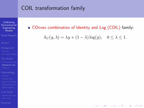
COIL transformation family
COnvex combination of Identity and Log (COIL) family:
hC (y, λ) = λy + (1− λ) log(y), 0 ≤ λ ≤ 1.
We restrict λ to [0, 1), since hC (·, 1) does not map (0,∞)to (−∞,∞)COIL can approximate Box-Cox:
For each λ ∈ [0, 1) there are constants λ′ ∈ [0, 1) anda, b ∈ R such that
hBC (y, λ) ≈ a + b hC (y, λ′)
for a wide range of y values (verified empirically)
The inverse h−1C (·, λ) does not have a closed form
evaluate by interpolation (fast)

CalibratingEnvironmental
EngineeringModels
David Ruppert
Outline
BackgroundThe team
The research problem
The ModelEnvironmental model
Modeling the noise
Likelihood
MethodologyOverview
Locating mode
Experimental Design
RBF approximation
MCMC sampling
Case StudyChemical spill model
Monte Carlo
Summary
COIL transformation family
COnvex combination of Identity and Log (COIL) family:
hC (y, λ) = λy + (1− λ) log(y), 0 ≤ λ ≤ 1.
We restrict λ to [0, 1), since hC (·, 1) does not map (0,∞)to (−∞,∞)
COIL can approximate Box-Cox:
For each λ ∈ [0, 1) there are constants λ′ ∈ [0, 1) anda, b ∈ R such that
hBC (y, λ) ≈ a + b hC (y, λ′)
for a wide range of y values (verified empirically)
The inverse h−1C (·, λ) does not have a closed form
evaluate by interpolation (fast)

CalibratingEnvironmental
EngineeringModels
David Ruppert
Outline
BackgroundThe team
The research problem
The ModelEnvironmental model
Modeling the noise
Likelihood
MethodologyOverview
Locating mode
Experimental Design
RBF approximation
MCMC sampling
Case StudyChemical spill model
Monte Carlo
Summary
COIL transformation family
COnvex combination of Identity and Log (COIL) family:
hC (y, λ) = λy + (1− λ) log(y), 0 ≤ λ ≤ 1.
We restrict λ to [0, 1), since hC (·, 1) does not map (0,∞)to (−∞,∞)COIL can approximate Box-Cox:
For each λ ∈ [0, 1) there are constants λ′ ∈ [0, 1) anda, b ∈ R such that
hBC (y, λ) ≈ a + b hC (y, λ′)
for a wide range of y values (verified empirically)The inverse h−1
C (·, λ) does not have a closed form
evaluate by interpolation (fast)

CalibratingEnvironmental
EngineeringModels
David Ruppert
Outline
BackgroundThe team
The research problem
The ModelEnvironmental model
Modeling the noise
Likelihood
MethodologyOverview
Locating mode
Experimental Design
RBF approximation
MCMC sampling
Case StudyChemical spill model
Monte Carlo
Summary
COIL transformation family
COnvex combination of Identity and Log (COIL) family:
hC (y, λ) = λy + (1− λ) log(y), 0 ≤ λ ≤ 1.
We restrict λ to [0, 1), since hC (·, 1) does not map (0,∞)to (−∞,∞)COIL can approximate Box-Cox:
For each λ ∈ [0, 1) there are constants λ′ ∈ [0, 1) anda, b ∈ R such that
hBC (y, λ) ≈ a + b hC (y, λ′)
for a wide range of y values (verified empirically)The inverse h−1
C (·, λ) does not have a closed formevaluate by interpolation (fast)

CalibratingEnvironmental
EngineeringModels
David Ruppert
Outline
BackgroundThe team
The research problem
The ModelEnvironmental model
Modeling the noise
Likelihood
MethodologyOverview
Locating mode
Experimental Design
RBF approximation
MCMC sampling
Case StudyChemical spill model
Monte Carlo
Summary
Multivariate transformations
Defineλ = (λ1, . . . , λd)T
andh(y,λ) = {h(y1, λ1), . . . , h(yd , λd)}T

CalibratingEnvironmental
EngineeringModels
David Ruppert
Outline
BackgroundThe team
The research problem
The ModelEnvironmental model
Modeling the noise
Likelihood
MethodologyOverview
Locating mode
Experimental Design
RBF approximation
MCMC sampling
Case StudyChemical spill model
Monte Carlo
Summary
Separable correlation model
Define the noise vectors:εi = (εi,1, . . . , εi,d)T = h{Yi ,λ} − h{f (Xi ,β),λ}ε•,j = (ε1,j , . . . , εn,j)T
ε = (εT1 , . . . , εT
n )T
cov(εi,j , εi′,j′) = C j,j′ · ρST (Xi , Xi′ ;γ)C is a d × d covariance matrix for εiρST(Xi , Xi′ ;γ) is a space-time correlation functionparameterized by γ
Var{ε} = Σ(θ) = S(γ)⊗Cθ = (γ, C)S i,i′(γ) = ρST(Xi , Xi′ ;γ)

CalibratingEnvironmental
EngineeringModels
David Ruppert
Outline
BackgroundThe team
The research problem
The ModelEnvironmental model
Modeling the noise
Likelihood
MethodologyOverview
Locating mode
Experimental Design
RBF approximation
MCMC sampling
Case StudyChemical spill model
Monte Carlo
Summary
TBS Likelihood
Our statistical model ish{Y ,λ} ∼ MVN [h{f (β),λ},Σ(θ)]Likelihood is
[Y |β,λ,θ] =
exp[−0.5 ‖h(Y ,λ)− h{f (β),λ}‖2
Σ(θ)−1
](2π)nd/2|Σ(θ)|1/2 · |Jh(Y ,λ)|
|Jh(Y ,λ)| is the JacobianΣ(θ) is the covariance matrix

CalibratingEnvironmental
EngineeringModels
David Ruppert
Outline
BackgroundThe team
The research problem
The ModelEnvironmental model
Modeling the noise
Likelihood
MethodologyOverview
Locating mode
Experimental Design
RBF approximation
MCMC sampling
Case StudyChemical spill model
Monte Carlo
Summary
Overview of Methodology
Goal:
Approximate the posterior density accurately with as fewexpensive likelihood evaluations as possible
There are four steps:
1 Locate the region(s) of high posterior density2 Find an “experimental design” that covers the region of
high posterior density
the likelihood is evaluated on this design
3 Use function evaluations from Steps 1 and 2 toapproximate the posterior
4 MCMC and standard Bayesian analysis using theapproximate posterior density

CalibratingEnvironmental
EngineeringModels
David Ruppert
Outline
BackgroundThe team
The research problem
The ModelEnvironmental model
Modeling the noise
Likelihood
MethodologyOverview
Locating mode
Experimental Design
RBF approximation
MCMC sampling
Case StudyChemical spill model
Monte Carlo
Summary
Overview of Methodology
Goal:Approximate the posterior density accurately with as fewexpensive likelihood evaluations as possible
There are four steps:1 Locate the region(s) of high posterior density
2 Find an “experimental design” that covers the region ofhigh posterior density
the likelihood is evaluated on this design
3 Use function evaluations from Steps 1 and 2 toapproximate the posterior
4 MCMC and standard Bayesian analysis using theapproximate posterior density

CalibratingEnvironmental
EngineeringModels
David Ruppert
Outline
BackgroundThe team
The research problem
The ModelEnvironmental model
Modeling the noise
Likelihood
MethodologyOverview
Locating mode
Experimental Design
RBF approximation
MCMC sampling
Case StudyChemical spill model
Monte Carlo
Summary
Overview of Methodology
Goal:Approximate the posterior density accurately with as fewexpensive likelihood evaluations as possible
There are four steps:1 Locate the region(s) of high posterior density2 Find an “experimental design” that covers the region of
high posterior density
the likelihood is evaluated on this design3 Use function evaluations from Steps 1 and 2 to
approximate the posterior4 MCMC and standard Bayesian analysis using the
approximate posterior density

CalibratingEnvironmental
EngineeringModels
David Ruppert
Outline
BackgroundThe team
The research problem
The ModelEnvironmental model
Modeling the noise
Likelihood
MethodologyOverview
Locating mode
Experimental Design
RBF approximation
MCMC sampling
Case StudyChemical spill model
Monte Carlo
Summary
Overview of Methodology
Goal:Approximate the posterior density accurately with as fewexpensive likelihood evaluations as possible
There are four steps:1 Locate the region(s) of high posterior density2 Find an “experimental design” that covers the region of
high posterior densitythe likelihood is evaluated on this design
3 Use function evaluations from Steps 1 and 2 toapproximate the posterior
4 MCMC and standard Bayesian analysis using theapproximate posterior density

CalibratingEnvironmental
EngineeringModels
David Ruppert
Outline
BackgroundThe team
The research problem
The ModelEnvironmental model
Modeling the noise
Likelihood
MethodologyOverview
Locating mode
Experimental Design
RBF approximation
MCMC sampling
Case StudyChemical spill model
Monte Carlo
Summary
Overview of Methodology
Goal:Approximate the posterior density accurately with as fewexpensive likelihood evaluations as possible
There are four steps:1 Locate the region(s) of high posterior density2 Find an “experimental design” that covers the region of
high posterior densitythe likelihood is evaluated on this design
3 Use function evaluations from Steps 1 and 2 toapproximate the posterior
4 MCMC and standard Bayesian analysis using theapproximate posterior density

CalibratingEnvironmental
EngineeringModels
David Ruppert
Outline
BackgroundThe team
The research problem
The ModelEnvironmental model
Modeling the noise
Likelihood
MethodologyOverview
Locating mode
Experimental Design
RBF approximation
MCMC sampling
Case StudyChemical spill model
Monte Carlo
Summary
Removing nuisance parameters
The posterior density is
[β,λ,θ|Y ] =[β,λ,θ, Y ]∫
[β,λ,θ, Y ] dβ dλ dθ,
where [β,λ,θ, Y ] = [Y |β,λ,θ] · [β,λ,θ]
Interest focuses on
[β|Y ] =∫
[β,λ,θ|Y ] dλ dθ

CalibratingEnvironmental
EngineeringModels
David Ruppert
Outline
BackgroundThe team
The research problem
The ModelEnvironmental model
Modeling the noise
Likelihood
MethodologyOverview
Locating mode
Experimental Design
RBF approximation
MCMC sampling
Case StudyChemical spill model
Monte Carlo
Summary
Removing nuisance parameters - four methods
Exact:[β|Y ] =
∫[β,λ,θ|Y ] dλ dθ
Profile posterior:
πmax(β, Y ) = supζ
[β, ζ, Y ] = [β, ζ(β), Y ]
ζ(β) maximizes [β, ζ, Y ] with respect to ζ
Laplace approximation:multiplies the profile posterior by a correction factor
Pseudo-posterior:[β, ζ(β), Y ]
{β, ζ(β)} is the MAP = joint mode of posterior

CalibratingEnvironmental
EngineeringModels
David Ruppert
Outline
BackgroundThe team
The research problem
The ModelEnvironmental model
Modeling the noise
Likelihood
MethodologyOverview
Locating mode
Experimental Design
RBF approximation
MCMC sampling
Case StudyChemical spill model
Monte Carlo
Summary
Finding posterior mode using Condor
When locating the posterior mode we want:
1 As few expensive function evaluations as possible2 A small percentage of “wasted evaluations”
a) few evaluation locations in region of very low posteriorprobability
b) few evaluation locations that are very close together
3 Getting very close to the mode is not a goalAll good optimization techniques achieve 1Optimization methods based on numerical derivativesviolate 2 b)
MATLAB’s fmincon exhibited this problem
CONDOR uses sequential quadratic programming
worked well in our empirical tests

CalibratingEnvironmental
EngineeringModels
David Ruppert
Outline
BackgroundThe team
The research problem
The ModelEnvironmental model
Modeling the noise
Likelihood
MethodologyOverview
Locating mode
Experimental Design
RBF approximation
MCMC sampling
Case StudyChemical spill model
Monte Carlo
Summary
Finding posterior mode using Condor
When locating the posterior mode we want:1 As few expensive function evaluations as possible
2 A small percentage of “wasted evaluations”
a) few evaluation locations in region of very low posteriorprobability
b) few evaluation locations that are very close together
3 Getting very close to the mode is not a goalAll good optimization techniques achieve 1Optimization methods based on numerical derivativesviolate 2 b)
MATLAB’s fmincon exhibited this problem
CONDOR uses sequential quadratic programming
worked well in our empirical tests

CalibratingEnvironmental
EngineeringModels
David Ruppert
Outline
BackgroundThe team
The research problem
The ModelEnvironmental model
Modeling the noise
Likelihood
MethodologyOverview
Locating mode
Experimental Design
RBF approximation
MCMC sampling
Case StudyChemical spill model
Monte Carlo
Summary
Finding posterior mode using Condor
When locating the posterior mode we want:1 As few expensive function evaluations as possible2 A small percentage of “wasted evaluations”
a) few evaluation locations in region of very low posteriorprobability
b) few evaluation locations that are very close together3 Getting very close to the mode is not a goal
All good optimization techniques achieve 1Optimization methods based on numerical derivativesviolate 2 b)
MATLAB’s fmincon exhibited this problem
CONDOR uses sequential quadratic programming
worked well in our empirical tests

CalibratingEnvironmental
EngineeringModels
David Ruppert
Outline
BackgroundThe team
The research problem
The ModelEnvironmental model
Modeling the noise
Likelihood
MethodologyOverview
Locating mode
Experimental Design
RBF approximation
MCMC sampling
Case StudyChemical spill model
Monte Carlo
Summary
Finding posterior mode using Condor
When locating the posterior mode we want:1 As few expensive function evaluations as possible2 A small percentage of “wasted evaluations”
a) few evaluation locations in region of very low posteriorprobability
b) few evaluation locations that are very close together
3 Getting very close to the mode is not a goalAll good optimization techniques achieve 1Optimization methods based on numerical derivativesviolate 2 b)
MATLAB’s fmincon exhibited this problem
CONDOR uses sequential quadratic programming
worked well in our empirical tests

CalibratingEnvironmental
EngineeringModels
David Ruppert
Outline
BackgroundThe team
The research problem
The ModelEnvironmental model
Modeling the noise
Likelihood
MethodologyOverview
Locating mode
Experimental Design
RBF approximation
MCMC sampling
Case StudyChemical spill model
Monte Carlo
Summary
Finding posterior mode using Condor
When locating the posterior mode we want:1 As few expensive function evaluations as possible2 A small percentage of “wasted evaluations”
a) few evaluation locations in region of very low posteriorprobability
b) few evaluation locations that are very close together3 Getting very close to the mode is not a goal
All good optimization techniques achieve 1Optimization methods based on numerical derivativesviolate 2 b)
MATLAB’s fmincon exhibited this problem
CONDOR uses sequential quadratic programming
worked well in our empirical tests

CalibratingEnvironmental
EngineeringModels
David Ruppert
Outline
BackgroundThe team
The research problem
The ModelEnvironmental model
Modeling the noise
Likelihood
MethodologyOverview
Locating mode
Experimental Design
RBF approximation
MCMC sampling
Case StudyChemical spill model
Monte Carlo
Summary
Finding posterior mode using Condor
When locating the posterior mode we want:1 As few expensive function evaluations as possible2 A small percentage of “wasted evaluations”
a) few evaluation locations in region of very low posteriorprobability
b) few evaluation locations that are very close together3 Getting very close to the mode is not a goal
All good optimization techniques achieve 1
Optimization methods based on numerical derivativesviolate 2 b)
MATLAB’s fmincon exhibited this problem
CONDOR uses sequential quadratic programming
worked well in our empirical tests

CalibratingEnvironmental
EngineeringModels
David Ruppert
Outline
BackgroundThe team
The research problem
The ModelEnvironmental model
Modeling the noise
Likelihood
MethodologyOverview
Locating mode
Experimental Design
RBF approximation
MCMC sampling
Case StudyChemical spill model
Monte Carlo
Summary
Finding posterior mode using Condor
When locating the posterior mode we want:1 As few expensive function evaluations as possible2 A small percentage of “wasted evaluations”
a) few evaluation locations in region of very low posteriorprobability
b) few evaluation locations that are very close together3 Getting very close to the mode is not a goal
All good optimization techniques achieve 1Optimization methods based on numerical derivativesviolate 2 b)
MATLAB’s fmincon exhibited this problemCONDOR uses sequential quadratic programming
worked well in our empirical tests

CalibratingEnvironmental
EngineeringModels
David Ruppert
Outline
BackgroundThe team
The research problem
The ModelEnvironmental model
Modeling the noise
Likelihood
MethodologyOverview
Locating mode
Experimental Design
RBF approximation
MCMC sampling
Case StudyChemical spill model
Monte Carlo
Summary
Finding posterior mode using Condor
When locating the posterior mode we want:1 As few expensive function evaluations as possible2 A small percentage of “wasted evaluations”
a) few evaluation locations in region of very low posteriorprobability
b) few evaluation locations that are very close together3 Getting very close to the mode is not a goal
All good optimization techniques achieve 1Optimization methods based on numerical derivativesviolate 2 b)
MATLAB’s fmincon exhibited this problemCONDOR uses sequential quadratic programming
worked well in our empirical tests

CalibratingEnvironmental
EngineeringModels
David Ruppert
Outline
BackgroundThe team
The research problem
The ModelEnvironmental model
Modeling the noise
Likelihood
MethodologyOverview
Locating mode
Experimental Design
RBF approximation
MCMC sampling
Case StudyChemical spill model
Monte Carlo
Summary
Further function evaluations needed
Goal:approximate posterior on CR(α) = {β : [β, Y ] > κ(α)}
Function evaluations in optimization stage insufficient toapproximate posterior accurately

CalibratingEnvironmental
EngineeringModels
David Ruppert
Outline
BackgroundThe team
The research problem
The ModelEnvironmental model
Modeling the noise
Likelihood
MethodologyOverview
Locating mode
Experimental Design
RBF approximation
MCMC sampling
Case StudyChemical spill model
Monte Carlo
Summary
Constructing the experimental design
1 Normal approximation to posterior
requires a small number of additional function evaluations2
CR(α) ={
β : (β − β)T[I
ββ]−1
(β − β) ≤ χ2p,1−α
}3 Space-filling design on CR(α)4 Remove points not in CR(α′) for α′ < α
E.g., α = 0.1 and α′ = 0.01

CalibratingEnvironmental
EngineeringModels
David Ruppert
Outline
BackgroundThe team
The research problem
The ModelEnvironmental model
Modeling the noise
Likelihood
MethodologyOverview
Locating mode
Experimental Design
RBF approximation
MCMC sampling
Case StudyChemical spill model
Monte Carlo
Summary
Constructing the experimental design
1 Normal approximation to posteriorrequires a small number of additional function evaluations
2
CR(α) ={
β : (β − β)T[I
ββ]−1
(β − β) ≤ χ2p,1−α
}
3 Space-filling design on CR(α)4 Remove points not in CR(α′) for α′ < α
E.g., α = 0.1 and α′ = 0.01

CalibratingEnvironmental
EngineeringModels
David Ruppert
Outline
BackgroundThe team
The research problem
The ModelEnvironmental model
Modeling the noise
Likelihood
MethodologyOverview
Locating mode
Experimental Design
RBF approximation
MCMC sampling
Case StudyChemical spill model
Monte Carlo
Summary
Constructing the experimental design
1 Normal approximation to posteriorrequires a small number of additional function evaluations
2
CR(α) ={
β : (β − β)T[I
ββ]−1
(β − β) ≤ χ2p,1−α
}3 Space-filling design on CR(α)
4 Remove points not in CR(α′) for α′ < α
E.g., α = 0.1 and α′ = 0.01

CalibratingEnvironmental
EngineeringModels
David Ruppert
Outline
BackgroundThe team
The research problem
The ModelEnvironmental model
Modeling the noise
Likelihood
MethodologyOverview
Locating mode
Experimental Design
RBF approximation
MCMC sampling
Case StudyChemical spill model
Monte Carlo
Summary
Constructing the experimental design
1 Normal approximation to posteriorrequires a small number of additional function evaluations
2
CR(α) ={
β : (β − β)T[I
ββ]−1
(β − β) ≤ χ2p,1−α
}3 Space-filling design on CR(α)4 Remove points not in CR(α′) for α′ < α
E.g., α = 0.1 and α′ = 0.01

CalibratingEnvironmental
EngineeringModels
David Ruppert
Outline
BackgroundThe team
The research problem
The ModelEnvironmental model
Modeling the noise
Likelihood
MethodologyOverview
Locating mode
Experimental Design
RBF approximation
MCMC sampling
Case StudyChemical spill model
Monte Carlo
Summary
Constructing the experimental design
1 Normal approximation to posteriorrequires a small number of additional function evaluations
2
CR(α) ={
β : (β − β)T[I
ββ]−1
(β − β) ≤ χ2p,1−α
}3 Space-filling design on CR(α)4 Remove points not in CR(α′) for α′ < α
E.g., α = 0.1 and α′ = 0.01

CalibratingEnvironmental
EngineeringModels
David Ruppert
Outline
BackgroundThe team
The research problem
The ModelEnvironmental model
Modeling the noise
Likelihood
MethodologyOverview
Locating mode
Experimental Design
RBF approximation
MCMC sampling
Case StudyChemical spill model
Monte Carlo
Summary
Radial basis functions
π(·, Y ) denotes one of the approximations to [β, Y ]
l(·) = log{π(·, Y )} is interpolated atBD = {β(1), . . . ,β(N)} by
l(β) =N∑
i=1aiφ(‖β − β(i)‖2) + q(β)
wherea1, . . . , aN ∈ Rφ is a radial basis function
we used φ(r) = r3
q ∈ Πpm (the space of polynomials in Rp of degree ≤ m
β ∈ Rp

CalibratingEnvironmental
EngineeringModels
David Ruppert
Outline
BackgroundThe team
The research problem
The ModelEnvironmental model
Modeling the noise
Likelihood
MethodologyOverview
Locating mode
Experimental Design
RBF approximation
MCMC sampling
Case StudyChemical spill model
Monte Carlo
Summary
Radial basis functions
π(·, Y ) denotes one of the approximations to [β, Y ]l(·) = log{π(·, Y )} is interpolated atBD = {β(1), . . . ,β(N)} by
l(β) =N∑
i=1aiφ(‖β − β(i)‖2) + q(β)
wherea1, . . . , aN ∈ Rφ is a radial basis function
we used φ(r) = r3
q ∈ Πpm (the space of polynomials in Rp of degree ≤ m
β ∈ Rp

CalibratingEnvironmental
EngineeringModels
David Ruppert
Outline
BackgroundThe team
The research problem
The ModelEnvironmental model
Modeling the noise
Likelihood
MethodologyOverview
Locating mode
Experimental Design
RBF approximation
MCMC sampling
Case StudyChemical spill model
Monte Carlo
Summary
Autoregressive Metropolis-Hastings algorithm
draw MCMC sample from π(·, Y ) = exp{l(·)}
restrict sample to CR(α′)Metropolis-Hastings candidate:βc = µ + ρ(β(t) − µ) + et
µ = location parameterρ = autoregressive parameter (matrix)
ρ = 0 → independence MHρ = 1 → random-walk MH
et ’s are i.i.d. from density g
if the candidate is accepted, then β(t+1) = βc
otherwise, β(t+1) = β(t)

CalibratingEnvironmental
EngineeringModels
David Ruppert
Outline
BackgroundThe team
The research problem
The ModelEnvironmental model
Modeling the noise
Likelihood
MethodologyOverview
Locating mode
Experimental Design
RBF approximation
MCMC sampling
Case StudyChemical spill model
Monte Carlo
Summary
Autoregressive Metropolis-Hastings algorithm
draw MCMC sample from π(·, Y ) = exp{l(·)}restrict sample to CR(α′)
Metropolis-Hastings candidate:βc = µ + ρ(β(t) − µ) + et
µ = location parameterρ = autoregressive parameter (matrix)
ρ = 0 → independence MHρ = 1 → random-walk MH
et ’s are i.i.d. from density gif the candidate is accepted, then β(t+1) = βc
otherwise, β(t+1) = β(t)

CalibratingEnvironmental
EngineeringModels
David Ruppert
Outline
BackgroundThe team
The research problem
The ModelEnvironmental model
Modeling the noise
Likelihood
MethodologyOverview
Locating mode
Experimental Design
RBF approximation
MCMC sampling
Case StudyChemical spill model
Monte Carlo
Summary
Autoregressive Metropolis-Hastings algorithm
draw MCMC sample from π(·, Y ) = exp{l(·)}restrict sample to CR(α′)
Metropolis-Hastings candidate:βc = µ + ρ(β(t) − µ) + et
µ = location parameter
ρ = autoregressive parameter (matrix)
ρ = 0 → independence MHρ = 1 → random-walk MH
et ’s are i.i.d. from density gif the candidate is accepted, then β(t+1) = βc
otherwise, β(t+1) = β(t)

CalibratingEnvironmental
EngineeringModels
David Ruppert
Outline
BackgroundThe team
The research problem
The ModelEnvironmental model
Modeling the noise
Likelihood
MethodologyOverview
Locating mode
Experimental Design
RBF approximation
MCMC sampling
Case StudyChemical spill model
Monte Carlo
Summary
Autoregressive Metropolis-Hastings algorithm
draw MCMC sample from π(·, Y ) = exp{l(·)}restrict sample to CR(α′)
Metropolis-Hastings candidate:βc = µ + ρ(β(t) − µ) + et
µ = location parameterρ = autoregressive parameter (matrix)
ρ = 0 → independence MHρ = 1 → random-walk MH
et ’s are i.i.d. from density gif the candidate is accepted, then β(t+1) = βc
otherwise, β(t+1) = β(t)

CalibratingEnvironmental
EngineeringModels
David Ruppert
Outline
BackgroundThe team
The research problem
The ModelEnvironmental model
Modeling the noise
Likelihood
MethodologyOverview
Locating mode
Experimental Design
RBF approximation
MCMC sampling
Case StudyChemical spill model
Monte Carlo
Summary
Autoregressive Metropolis-Hastings algorithm
draw MCMC sample from π(·, Y ) = exp{l(·)}restrict sample to CR(α′)
Metropolis-Hastings candidate:βc = µ + ρ(β(t) − µ) + et
µ = location parameterρ = autoregressive parameter (matrix)
ρ = 0 → independence MH
ρ = 1 → random-walk MHet ’s are i.i.d. from density g
if the candidate is accepted, then β(t+1) = βc
otherwise, β(t+1) = β(t)

CalibratingEnvironmental
EngineeringModels
David Ruppert
Outline
BackgroundThe team
The research problem
The ModelEnvironmental model
Modeling the noise
Likelihood
MethodologyOverview
Locating mode
Experimental Design
RBF approximation
MCMC sampling
Case StudyChemical spill model
Monte Carlo
Summary
Autoregressive Metropolis-Hastings algorithm
draw MCMC sample from π(·, Y ) = exp{l(·)}restrict sample to CR(α′)
Metropolis-Hastings candidate:βc = µ + ρ(β(t) − µ) + et
µ = location parameterρ = autoregressive parameter (matrix)
ρ = 0 → independence MHρ = 1 → random-walk MH
et ’s are i.i.d. from density gif the candidate is accepted, then β(t+1) = βc
otherwise, β(t+1) = β(t)

CalibratingEnvironmental
EngineeringModels
David Ruppert
Outline
BackgroundThe team
The research problem
The ModelEnvironmental model
Modeling the noise
Likelihood
MethodologyOverview
Locating mode
Experimental Design
RBF approximation
MCMC sampling
Case StudyChemical spill model
Monte Carlo
Summary
Autoregressive Metropolis-Hastings algorithm
draw MCMC sample from π(·, Y ) = exp{l(·)}restrict sample to CR(α′)
Metropolis-Hastings candidate:βc = µ + ρ(β(t) − µ) + et
µ = location parameterρ = autoregressive parameter (matrix)
ρ = 0 → independence MHρ = 1 → random-walk MH
et ’s are i.i.d. from density g
if the candidate is accepted, then β(t+1) = βc
otherwise, β(t+1) = β(t)

CalibratingEnvironmental
EngineeringModels
David Ruppert
Outline
BackgroundThe team
The research problem
The ModelEnvironmental model
Modeling the noise
Likelihood
MethodologyOverview
Locating mode
Experimental Design
RBF approximation
MCMC sampling
Case StudyChemical spill model
Monte Carlo
Summary
Autoregressive Metropolis-Hastings algorithm
draw MCMC sample from π(·, Y ) = exp{l(·)}restrict sample to CR(α′)
Metropolis-Hastings candidate:βc = µ + ρ(β(t) − µ) + et
µ = location parameterρ = autoregressive parameter (matrix)
ρ = 0 → independence MHρ = 1 → random-walk MH
et ’s are i.i.d. from density gif the candidate is accepted, then β(t+1) = βc
otherwise, β(t+1) = β(t)

CalibratingEnvironmental
EngineeringModels
David Ruppert
Outline
BackgroundThe team
The research problem
The ModelEnvironmental model
Modeling the noise
Likelihood
MethodologyOverview
Locating mode
Experimental Design
RBF approximation
MCMC sampling
Case StudyChemical spill model
Monte Carlo
Summary
Autoregressive Metropolis-Hastings algorithm
draw MCMC sample from π(·, Y ) = exp{l(·)}restrict sample to CR(α′)
Metropolis-Hastings candidate:βc = µ + ρ(β(t) − µ) + et
µ = location parameterρ = autoregressive parameter (matrix)
ρ = 0 → independence MHρ = 1 → random-walk MH
et ’s are i.i.d. from density gif the candidate is accepted, then β(t+1) = βc
otherwise, β(t+1) = β(t)

CalibratingEnvironmental
EngineeringModels
David Ruppert
Outline
BackgroundThe team
The research problem
The ModelEnvironmental model
Modeling the noise
Likelihood
MethodologyOverview
Locating mode
Experimental Design
RBF approximation
MCMC sampling
Case StudyChemical spill model
Monte Carlo
Summary
Applications in Environmental Engineering
few statisticians are working on environmental engineeringproblems
environmental engineers typically use ad hoc andinefficient statistical methodsmodern statistical techniques such as variance functions,transformations, spatial-temporal models potentially offersubstantial improvements

CalibratingEnvironmental
EngineeringModels
David Ruppert
Outline
BackgroundThe team
The research problem
The ModelEnvironmental model
Modeling the noise
Likelihood
MethodologyOverview
Locating mode
Experimental Design
RBF approximation
MCMC sampling
Case StudyChemical spill model
Monte Carlo
Summary
Applications in Environmental Engineering
few statisticians are working on environmental engineeringproblemsenvironmental engineers typically use ad hoc andinefficient statistical methods
modern statistical techniques such as variance functions,transformations, spatial-temporal models potentially offersubstantial improvements

CalibratingEnvironmental
EngineeringModels
David Ruppert
Outline
BackgroundThe team
The research problem
The ModelEnvironmental model
Modeling the noise
Likelihood
MethodologyOverview
Locating mode
Experimental Design
RBF approximation
MCMC sampling
Case StudyChemical spill model
Monte Carlo
Summary
Applications in Environmental Engineering
few statisticians are working on environmental engineeringproblemsenvironmental engineers typically use ad hoc andinefficient statistical methodsmodern statistical techniques such as variance functions,transformations, spatial-temporal models potentially offersubstantial improvements

CalibratingEnvironmental
EngineeringModels
David Ruppert
Outline
BackgroundThe team
The research problem
The ModelEnvironmental model
Modeling the noise
Likelihood
MethodologyOverview
Locating mode
Experimental Design
RBF approximation
MCMC sampling
Case StudyChemical spill model
Monte Carlo
Summary
GLUE
GLUE = Generalized Likelihood Uncertainty Estimation
widely usedapparently considered state-of-the-art by manyenvironmental engineersreplaces the likelihood function of iid normal errors withan arbitrary objective functionshows no appreciation of maximum likelihood as a generalmethodobjective function is not based on the data-generatingprobability model

CalibratingEnvironmental
EngineeringModels
David Ruppert
Outline
BackgroundThe team
The research problem
The ModelEnvironmental model
Modeling the noise
Likelihood
MethodologyOverview
Locating mode
Experimental Design
RBF approximation
MCMC sampling
Case StudyChemical spill model
Monte Carlo
Summary
GLUE
GLUE = Generalized Likelihood Uncertainty Estimationwidely used
apparently considered state-of-the-art by manyenvironmental engineersreplaces the likelihood function of iid normal errors withan arbitrary objective functionshows no appreciation of maximum likelihood as a generalmethodobjective function is not based on the data-generatingprobability model

CalibratingEnvironmental
EngineeringModels
David Ruppert
Outline
BackgroundThe team
The research problem
The ModelEnvironmental model
Modeling the noise
Likelihood
MethodologyOverview
Locating mode
Experimental Design
RBF approximation
MCMC sampling
Case StudyChemical spill model
Monte Carlo
Summary
GLUE
GLUE = Generalized Likelihood Uncertainty Estimationwidely usedapparently considered state-of-the-art by manyenvironmental engineers
replaces the likelihood function of iid normal errors withan arbitrary objective functionshows no appreciation of maximum likelihood as a generalmethodobjective function is not based on the data-generatingprobability model

CalibratingEnvironmental
EngineeringModels
David Ruppert
Outline
BackgroundThe team
The research problem
The ModelEnvironmental model
Modeling the noise
Likelihood
MethodologyOverview
Locating mode
Experimental Design
RBF approximation
MCMC sampling
Case StudyChemical spill model
Monte Carlo
Summary
GLUE
GLUE = Generalized Likelihood Uncertainty Estimationwidely usedapparently considered state-of-the-art by manyenvironmental engineersreplaces the likelihood function of iid normal errors withan arbitrary objective function
shows no appreciation of maximum likelihood as a generalmethodobjective function is not based on the data-generatingprobability model

CalibratingEnvironmental
EngineeringModels
David Ruppert
Outline
BackgroundThe team
The research problem
The ModelEnvironmental model
Modeling the noise
Likelihood
MethodologyOverview
Locating mode
Experimental Design
RBF approximation
MCMC sampling
Case StudyChemical spill model
Monte Carlo
Summary
GLUE
GLUE = Generalized Likelihood Uncertainty Estimationwidely usedapparently considered state-of-the-art by manyenvironmental engineersreplaces the likelihood function of iid normal errors withan arbitrary objective functionshows no appreciation of maximum likelihood as a generalmethod
objective function is not based on the data-generatingprobability model

CalibratingEnvironmental
EngineeringModels
David Ruppert
Outline
BackgroundThe team
The research problem
The ModelEnvironmental model
Modeling the noise
Likelihood
MethodologyOverview
Locating mode
Experimental Design
RBF approximation
MCMC sampling
Case StudyChemical spill model
Monte Carlo
Summary
GLUE
GLUE = Generalized Likelihood Uncertainty Estimationwidely usedapparently considered state-of-the-art by manyenvironmental engineersreplaces the likelihood function of iid normal errors withan arbitrary objective functionshows no appreciation of maximum likelihood as a generalmethodobjective function is not based on the data-generatingprobability model

CalibratingEnvironmental
EngineeringModels
David Ruppert
Outline
BackgroundThe team
The research problem
The ModelEnvironmental model
Modeling the noise
Likelihood
MethodologyOverview
Locating mode
Experimental Design
RBF approximation
MCMC sampling
Case StudyChemical spill model
Monte Carlo
Summary
Synthetic data example: Chemical spill
To test algorithm:
use computationally inexpensive functionthen approximate and exact result can be compared
chemical accident caused spill at two locations on a longchannel
mass M spill at location 0 at time 0mass M spill at location L and time τ
diffusion coefficient is dparameter vector is β = (m, d, l, τ)T
want estimate of average concentration at end of channell is of special interestneed assessments of uncertainty as well

CalibratingEnvironmental
EngineeringModels
David Ruppert
Outline
BackgroundThe team
The research problem
The ModelEnvironmental model
Modeling the noise
Likelihood
MethodologyOverview
Locating mode
Experimental Design
RBF approximation
MCMC sampling
Case StudyChemical spill model
Monte Carlo
Summary
Synthetic data example: Chemical spill
To test algorithm:use computationally inexpensive function
then approximate and exact result can be comparedchemical accident caused spill at two locations on a longchannel
mass M spill at location 0 at time 0mass M spill at location L and time τ
diffusion coefficient is dparameter vector is β = (m, d, l, τ)T
want estimate of average concentration at end of channell is of special interestneed assessments of uncertainty as well

CalibratingEnvironmental
EngineeringModels
David Ruppert
Outline
BackgroundThe team
The research problem
The ModelEnvironmental model
Modeling the noise
Likelihood
MethodologyOverview
Locating mode
Experimental Design
RBF approximation
MCMC sampling
Case StudyChemical spill model
Monte Carlo
Summary
Synthetic data example: Chemical spill
To test algorithm:use computationally inexpensive functionthen approximate and exact result can be compared
chemical accident caused spill at two locations on a longchannel
mass M spill at location 0 at time 0mass M spill at location L and time τ
diffusion coefficient is dparameter vector is β = (m, d, l, τ)T
want estimate of average concentration at end of channell is of special interestneed assessments of uncertainty as well

CalibratingEnvironmental
EngineeringModels
David Ruppert
Outline
BackgroundThe team
The research problem
The ModelEnvironmental model
Modeling the noise
Likelihood
MethodologyOverview
Locating mode
Experimental Design
RBF approximation
MCMC sampling
Case StudyChemical spill model
Monte Carlo
Summary
Synthetic data example: Chemical spill
To test algorithm:use computationally inexpensive functionthen approximate and exact result can be compared
chemical accident caused spill at two locations on a longchannel
mass M spill at location 0 at time 0
mass M spill at location L and time τ
diffusion coefficient is dparameter vector is β = (m, d, l, τ)T
want estimate of average concentration at end of channell is of special interestneed assessments of uncertainty as well

CalibratingEnvironmental
EngineeringModels
David Ruppert
Outline
BackgroundThe team
The research problem
The ModelEnvironmental model
Modeling the noise
Likelihood
MethodologyOverview
Locating mode
Experimental Design
RBF approximation
MCMC sampling
Case StudyChemical spill model
Monte Carlo
Summary
Synthetic data example: Chemical spill
To test algorithm:use computationally inexpensive functionthen approximate and exact result can be compared
chemical accident caused spill at two locations on a longchannel
mass M spill at location 0 at time 0mass M spill at location L and time τ
diffusion coefficient is dparameter vector is β = (m, d, l, τ)T
want estimate of average concentration at end of channell is of special interestneed assessments of uncertainty as well

CalibratingEnvironmental
EngineeringModels
David Ruppert
Outline
BackgroundThe team
The research problem
The ModelEnvironmental model
Modeling the noise
Likelihood
MethodologyOverview
Locating mode
Experimental Design
RBF approximation
MCMC sampling
Case StudyChemical spill model
Monte Carlo
Summary
Synthetic data example: Chemical spill
To test algorithm:use computationally inexpensive functionthen approximate and exact result can be compared
chemical accident caused spill at two locations on a longchannel
mass M spill at location 0 at time 0mass M spill at location L and time τ
diffusion coefficient is d
parameter vector is β = (m, d, l, τ)T
want estimate of average concentration at end of channell is of special interestneed assessments of uncertainty as well

CalibratingEnvironmental
EngineeringModels
David Ruppert
Outline
BackgroundThe team
The research problem
The ModelEnvironmental model
Modeling the noise
Likelihood
MethodologyOverview
Locating mode
Experimental Design
RBF approximation
MCMC sampling
Case StudyChemical spill model
Monte Carlo
Summary
Synthetic data example: Chemical spill
To test algorithm:use computationally inexpensive functionthen approximate and exact result can be compared
chemical accident caused spill at two locations on a longchannel
mass M spill at location 0 at time 0mass M spill at location L and time τ
diffusion coefficient is dparameter vector is β = (m, d, l, τ)T
want estimate of average concentration at end of channell is of special interestneed assessments of uncertainty as well

CalibratingEnvironmental
EngineeringModels
David Ruppert
Outline
BackgroundThe team
The research problem
The ModelEnvironmental model
Modeling the noise
Likelihood
MethodologyOverview
Locating mode
Experimental Design
RBF approximation
MCMC sampling
Case StudyChemical spill model
Monte Carlo
Summary
Synthetic data example: Chemical spill
To test algorithm:use computationally inexpensive functionthen approximate and exact result can be compared
chemical accident caused spill at two locations on a longchannel
mass M spill at location 0 at time 0mass M spill at location L and time τ
diffusion coefficient is dparameter vector is β = (m, d, l, τ)T
want estimate of average concentration at end of channel
l is of special interestneed assessments of uncertainty as well

CalibratingEnvironmental
EngineeringModels
David Ruppert
Outline
BackgroundThe team
The research problem
The ModelEnvironmental model
Modeling the noise
Likelihood
MethodologyOverview
Locating mode
Experimental Design
RBF approximation
MCMC sampling
Case StudyChemical spill model
Monte Carlo
Summary
Synthetic data example: Chemical spill
To test algorithm:use computationally inexpensive functionthen approximate and exact result can be compared
chemical accident caused spill at two locations on a longchannel
mass M spill at location 0 at time 0mass M spill at location L and time τ
diffusion coefficient is dparameter vector is β = (m, d, l, τ)T
want estimate of average concentration at end of channell is of special interest
need assessments of uncertainty as well

CalibratingEnvironmental
EngineeringModels
David Ruppert
Outline
BackgroundThe team
The research problem
The ModelEnvironmental model
Modeling the noise
Likelihood
MethodologyOverview
Locating mode
Experimental Design
RBF approximation
MCMC sampling
Case StudyChemical spill model
Monte Carlo
Summary
Synthetic data example: Chemical spill
To test algorithm:use computationally inexpensive functionthen approximate and exact result can be compared
chemical accident caused spill at two locations on a longchannel
mass M spill at location 0 at time 0mass M spill at location L and time τ
diffusion coefficient is dparameter vector is β = (m, d, l, τ)T
want estimate of average concentration at end of channell is of special interestneed assessments of uncertainty as well

CalibratingEnvironmental
EngineeringModels
David Ruppert
Outline
BackgroundThe team
The research problem
The ModelEnvironmental model
Modeling the noise
Likelihood
MethodologyOverview
Locating mode
Experimental Design
RBF approximation
MCMC sampling
Case StudyChemical spill model
Monte Carlo
Summary
Chemical spill model
Model is:
C(s, t; M , D, L, τ) =M
√4πDt
exp�−s2
4Dt
�
+Mp
4πD(t − τ)exp
�−(s − L)2
4D(t − τ)
�· I(τ < t)

CalibratingEnvironmental
EngineeringModels
David Ruppert
Outline
BackgroundThe team
The research problem
The ModelEnvironmental model
Modeling the noise
Likelihood
MethodologyOverview
Locating mode
Experimental Design
RBF approximation
MCMC sampling
Case StudyChemical spill model
Monte Carlo
Summary
Details of simulation
assume data is collected at spatial location 0 (0.5) 2.5 andtimes 0.3 (0.3) 60 (5 time 200 observations)assume that a major goal is to estimate averageconcentration of time interval [40, 140] at the end of thechannel (s = 3), specifically
F(β) =20∑
i=0f {(3, 40 + 5i),β}
requires additional function evaluations (but not muchmore computation)

CalibratingEnvironmental
EngineeringModels
David Ruppert
Outline
BackgroundThe team
The research problem
The ModelEnvironmental model
Modeling the noise
Likelihood
MethodologyOverview
Locating mode
Experimental Design
RBF approximation
MCMC sampling
Case StudyChemical spill model
Monte Carlo
Summary
Details, continued
λ = 0.333 in COIL familyone chemical speciesσ can be integrated out of the posterior analytically

CalibratingEnvironmental
EngineeringModels
David Ruppert
Outline
BackgroundThe team
The research problem
The ModelEnvironmental model
Modeling the noise
Likelihood
MethodologyOverview
Locating mode
Experimental Design
RBF approximation
MCMC sampling
Case StudyChemical spill model
Monte Carlo
Summary
Posterior densities: components of β
9.8 10 10.2 10.40
1
2
3
4
5
β1
0.065 0.0675 0.07 0.0725 0.0750
100
200
300
400
β2
0.94 0.96 0.98 1 1.02 1.04 1.060
5
10
15
20
25
30
β3
30.1 30.12 30.14 30.16 30.18 30.20
10
20
30
40
β4
Figure: Kernel estimates of the posterior densities of βi ’s with theexact joint posterior (solid line) and RBF approximations to jointposterior (dashed line), pseudoposterior (dashed-dotted line), profileposterior with and without Laplace correction (dotted and largedotted lines, respectively).

CalibratingEnvironmental
EngineeringModels
David Ruppert
Outline
BackgroundThe team
The research problem
The ModelEnvironmental model
Modeling the noise
Likelihood
MethodologyOverview
Locating mode
Experimental Design
RBF approximation
MCMC sampling
Case StudyChemical spill model
Monte Carlo
Summary
Posterior densities: F(β)
124 125 126 127 128 129 130 131 132 133 1340
0.05
0.1
0.15
0.2
0.25
0.3
0.35
F(β)
Figure: Kernel smoothed density estimates for the posterior of F(β).

CalibratingEnvironmental
EngineeringModels
David Ruppert
Outline
BackgroundThe team
The research problem
The ModelEnvironmental model
Modeling the noise
Likelihood
MethodologyOverview
Locating mode
Experimental Design
RBF approximation
MCMC sampling
Case StudyChemical spill model
Monte Carlo
Summary
Results of a Monte Carlo experiment
MC mean ratio of C.I. lengthstrue exact RBF size .9 size .95 size .99
β1 = M 10 10.0057 10.0061 .9969 .9961 .9844(.0866) (.0893) (.0602) (.0624) (.0738)
β2 = D .07 .07008 .07008 .9910 .9888 .9687(.00097) (.00101) (.0592) (.0612) (.0673)
β3 = L 1 1.0005 1.0005 .9671 .9662 .9604(.0136) (.0134) (.0785) (.0765) (.0750)
β4 = τ 30.16 30.1610 30.1610 .9786 .9709 .9403(.0096) (.0096) (.0779) (.0818) (.0835)
F(β) 128.998 129.063 129.067 .9959 .9937 .9841(1.087) (1.100) (.062) (.0628) (.0695)

CalibratingEnvironmental
EngineeringModels
David Ruppert
Outline
BackgroundThe team
The research problem
The ModelEnvironmental model
Modeling the noise
Likelihood
MethodologyOverview
Locating mode
Experimental Design
RBF approximation
MCMC sampling
Case StudyChemical spill model
Monte Carlo
Summary
Results of a Monte Carlo experiment
Table: Observed coverage probabilities.
size .9 cred. int. size .95 cred. int. size .99 cred. int.exact RBF exact RBF exact RBF
β1 .905 .904 .950 .944 .986 .990(.009) (.009) (.007) (.007) (.004) (.003)
β2 .908 .903 .954 .951 .991 .987(.009) (.009) (.007) (.007) (.003) (.004)
β3 .916 .899 .953 .954 .989 .988(.009) (.010) (.007) (.007) (.003) (.003)
β4 .904 .909 .947 .945 .988 .987(.009) (.009) (.007) (.007) (.003) (.004)
F(β) .904 .902 .947 .937 .994 .980(.009) (.009) (.007) (.008) (.002) (.004)

CalibratingEnvironmental
EngineeringModels
David Ruppert
Outline
BackgroundThe team
The research problem
The ModelEnvironmental model
Modeling the noise
Likelihood
MethodologyOverview
Locating mode
Experimental Design
RBF approximation
MCMC sampling
Case StudyChemical spill model
Monte Carlo
Summary
What have we achieved?
In this research we have:applied modern statistical tools to calibration ofenvironmental engineering models, e.g.,
transform-both-sidespatial-temporal correlation models
implemented a Bayesian method of uncertainty analysissubstantially reduced the number of evaluations of thecomputationally expensive environmental model

CalibratingEnvironmental
EngineeringModels
David Ruppert
Outline
BackgroundThe team
The research problem
The ModelEnvironmental model
Modeling the noise
Likelihood
MethodologyOverview
Locating mode
Experimental Design
RBF approximation
MCMC sampling
Case StudyChemical spill model
Monte Carlo
Summary
What have we achieved?
In this research we have:applied modern statistical tools to calibration ofenvironmental engineering models, e.g.,
transform-both-side
spatial-temporal correlation modelsimplemented a Bayesian method of uncertainty analysissubstantially reduced the number of evaluations of thecomputationally expensive environmental model

CalibratingEnvironmental
EngineeringModels
David Ruppert
Outline
BackgroundThe team
The research problem
The ModelEnvironmental model
Modeling the noise
Likelihood
MethodologyOverview
Locating mode
Experimental Design
RBF approximation
MCMC sampling
Case StudyChemical spill model
Monte Carlo
Summary
What have we achieved?
In this research we have:applied modern statistical tools to calibration ofenvironmental engineering models, e.g.,
transform-both-sidespatial-temporal correlation models
implemented a Bayesian method of uncertainty analysissubstantially reduced the number of evaluations of thecomputationally expensive environmental model

CalibratingEnvironmental
EngineeringModels
David Ruppert
Outline
BackgroundThe team
The research problem
The ModelEnvironmental model
Modeling the noise
Likelihood
MethodologyOverview
Locating mode
Experimental Design
RBF approximation
MCMC sampling
Case StudyChemical spill model
Monte Carlo
Summary
What have we achieved?
In this research we have:applied modern statistical tools to calibration ofenvironmental engineering models, e.g.,
transform-both-sidespatial-temporal correlation models
implemented a Bayesian method of uncertainty analysis
substantially reduced the number of evaluations of thecomputationally expensive environmental model

CalibratingEnvironmental
EngineeringModels
David Ruppert
Outline
BackgroundThe team
The research problem
The ModelEnvironmental model
Modeling the noise
Likelihood
MethodologyOverview
Locating mode
Experimental Design
RBF approximation
MCMC sampling
Case StudyChemical spill model
Monte Carlo
Summary
What have we achieved?
In this research we have:applied modern statistical tools to calibration ofenvironmental engineering models, e.g.,
transform-both-sidespatial-temporal correlation models
implemented a Bayesian method of uncertainty analysissubstantially reduced the number of evaluations of thecomputationally expensive environmental model

CalibratingEnvironmental
EngineeringModels
David Ruppert
Outline
BackgroundThe team
The research problem
The ModelEnvironmental model
Modeling the noise
Likelihood
MethodologyOverview
Locating mode
Experimental Design
RBF approximation
MCMC sampling
Case StudyChemical spill model
Monte Carlo
Summary
Race Brook, Nov 5, 2005