Embed Size (px)
Citation preview
Calculus on a Normed Linear Space
James S. CookLiberty University
Department of Mathematics
Fall 2017
2
introduction and scope
These notes are intended for someone who has completed the introductory calculus sequence andhas some experience with matrices or linear algebra. This set of notes covers the first month or so ofMath 332 at Liberty University. I intend this to serve as a supplement to our required text: FirstSteps in Differential Geometry: Riemannian, Contact, Symplectic by Andrew McInerney. Oncewe’ve covered these notes then we begin studying Chapter 3 of McInerney’s text.
This course is primarily concerned with abstractions of calculus and geometry which are accessibleto the undergraduate. This is not a course in real analysis and it does not have a prerequisite ofreal analysis so my typical students are not prepared for topology or measure theory. We deferthe topology of manifolds and exposition of abstract integration in the measure theoretic sense toanother course. Our focus for course as a whole is on what you might call the linear algebra ofabstract calculus. Indeed, McInerney essentially declares the same philosophy so his text is thenatural extension of what I share in these notes. So, what do we study here? In these notes:
How to generalize calculus to the context of a normed linear space
In particular, we study: basic linear algebra, spanning, linear independennce, basis, coordinates,norms, distance functions, inner products, metric topology, limits and their laws in a NLS, conti-nuity of mappings on NLS’s, linearization, Frechet derivatives, partial derivatives and continuousdifferentiability, linearization, properties of differentials, generalized chain and product rules, in-tuition and statement of inverse and implicit function theorems, implicit differentiation via themethod of differentials, manifolds in Rn from an implicit or parametric viewpoint, tangent and nor-mal spaces of a submanifold of Euclidean space, Lagrange multiplier technique, compact sets andthe extreme value theorem, theory of quadratic forms, proof of real Spectral Theorem via methodof Lagrange multipliers, higher derivatives and the multivariate Taylor theorem, multivariate powerseries, critical point analysis for multivariate functions, introduction to variational calculus.
In contrast to some previous versions of this course, I do not study contraction mappings, dif-ferentiating under the integral and other questions related to uniform convergence. I leave suchtopics to a future course which likely takes Math 431 (our real analysis course) as a prerequisite.Furthermore, these notes have little to say about further calculus (differential forms, vector fields,etc.). We read on those topics in McInerney once we exhaust these notes.
There are many excellent texts on calculus of many variables. Three which have had significantinfluence on my thinking and the creation of these notes are:
1. Advanced Calculus of Several Variables revised Dover Ed. by C.H. Edwards,
2. Mathematical Analysis II, Vladimir A. Zorich,
3. Foundations of Modern Analysis, by J. Dieudonne, Academic Press Inc. (1960)
These notes are a work in progress, do let me know about the errors. Thanks!
James S. Cook, August 14, 2017.
Contents
1 on norms and limits 5
1.1 linear algebra . . . . . . . . . . . . . . . . . . . . . . . . . . . . . . . . . . . . . . . . 6
1.2 norms, metrics and inner products . . . . . . . . . . . . . . . . . . . . . . . . . . . . 8
1.2.1 normed linear spaces . . . . . . . . . . . . . . . . . . . . . . . . . . . . . . . . 8
1.2.2 inner product space . . . . . . . . . . . . . . . . . . . . . . . . . . . . . . . . 11
1.2.3 metric as a distance function . . . . . . . . . . . . . . . . . . . . . . . . . . . 12
1.3 topology and limits in normed linear spaces . . . . . . . . . . . . . . . . . . . . . . . 12
1.4 sequential analysis . . . . . . . . . . . . . . . . . . . . . . . . . . . . . . . . . . . . . 22
2 differentiation 25
2.1 the Frechet differential . . . . . . . . . . . . . . . . . . . . . . . . . . . . . . . . . . . 26
2.2 properties of the Frechet derivative . . . . . . . . . . . . . . . . . . . . . . . . . . . . 32
2.3 partial derivatives of differentiable maps . . . . . . . . . . . . . . . . . . . . . . . . . 34
2.3.1 partial differentiation in a finite dimensional real vector space . . . . . . . . . 34
2.3.2 partial differentiation for real . . . . . . . . . . . . . . . . . . . . . . . . . . . 37
2.3.3 examples of Jacobian matrices . . . . . . . . . . . . . . . . . . . . . . . . . . 39
2.3.4 on chain rule and Jacobian matrix multiplication . . . . . . . . . . . . . . . . 43
2.4 continuous differentiability . . . . . . . . . . . . . . . . . . . . . . . . . . . . . . . . . 45
2.5 the product rule . . . . . . . . . . . . . . . . . . . . . . . . . . . . . . . . . . . . . . 49
2.6 higher derivatives . . . . . . . . . . . . . . . . . . . . . . . . . . . . . . . . . . . . . . 52
2.7 differentiation in an algebra variable . . . . . . . . . . . . . . . . . . . . . . . . . . . 52
3 inverse and implicit function theorems 55
3.1 inverse function theorem . . . . . . . . . . . . . . . . . . . . . . . . . . . . . . . . . . 55
3.2 implicit function theorem . . . . . . . . . . . . . . . . . . . . . . . . . . . . . . . . . 59
3.3 implicit differentiation . . . . . . . . . . . . . . . . . . . . . . . . . . . . . . . . . . . 68
3.3.1 computational techniques for partial differentiation with side conditions . . . 71
3.4 the constant rank theorem . . . . . . . . . . . . . . . . . . . . . . . . . . . . . . . . . 73
4 two views of manifolds in Rn 79
4.1 definition of level set . . . . . . . . . . . . . . . . . . . . . . . . . . . . . . . . . . . . 80
4.2 tangents and normals to a level set . . . . . . . . . . . . . . . . . . . . . . . . . . . . 81
4.3 tangent and normal space from patches . . . . . . . . . . . . . . . . . . . . . . . . . 86
4.4 summary of tangent and normal spaces . . . . . . . . . . . . . . . . . . . . . . . . . 87
4.5 method of Lagrange mulitpliers . . . . . . . . . . . . . . . . . . . . . . . . . . . . . . 88
3

4 CONTENTS
5 critical point analysis for several variables 935.1 multivariate power series . . . . . . . . . . . . . . . . . . . . . . . . . . . . . . . . . . 93
5.1.1 taylor’s polynomial for one-variable . . . . . . . . . . . . . . . . . . . . . . . . 935.1.2 taylor’s multinomial for two-variables . . . . . . . . . . . . . . . . . . . . . . 955.1.3 taylor’s multinomial for many-variables . . . . . . . . . . . . . . . . . . . . . 97
5.2 a brief introduction to the theory of quadratic forms . . . . . . . . . . . . . . . . . . 995.2.1 diagonalizing forms via eigenvectors . . . . . . . . . . . . . . . . . . . . . . . 102
5.3 second derivative test in many-variables . . . . . . . . . . . . . . . . . . . . . . . . . 109
6 introduction to variational calculus 1136.1 history . . . . . . . . . . . . . . . . . . . . . . . . . . . . . . . . . . . . . . . . . . . . 1136.2 the variational problem . . . . . . . . . . . . . . . . . . . . . . . . . . . . . . . . . . 1146.3 variational derivative . . . . . . . . . . . . . . . . . . . . . . . . . . . . . . . . . . . . 1166.4 Euler-Lagrange examples . . . . . . . . . . . . . . . . . . . . . . . . . . . . . . . . . 117
6.4.1 shortest distance between two points in plane . . . . . . . . . . . . . . . . . . 1176.4.2 surface of revolution with minimal area . . . . . . . . . . . . . . . . . . . . . 1186.4.3 Braichistochrone . . . . . . . . . . . . . . . . . . . . . . . . . . . . . . . . . . 119
6.5 Euler-Lagrange equations for several dependent variables . . . . . . . . . . . . . . . . 1206.5.1 free particle Lagrangian . . . . . . . . . . . . . . . . . . . . . . . . . . . . . . 1216.5.2 geodesics in R3 . . . . . . . . . . . . . . . . . . . . . . . . . . . . . . . . . . . 122
6.6 the Euclidean metric . . . . . . . . . . . . . . . . . . . . . . . . . . . . . . . . . . . . 1226.7 geodesics . . . . . . . . . . . . . . . . . . . . . . . . . . . . . . . . . . . . . . . . . . 124
6.7.1 geodesic on cylinder . . . . . . . . . . . . . . . . . . . . . . . . . . . . . . . . 1246.7.2 geodesic on sphere . . . . . . . . . . . . . . . . . . . . . . . . . . . . . . . . . 125
6.8 Lagrangian mechanics . . . . . . . . . . . . . . . . . . . . . . . . . . . . . . . . . . . 1256.8.1 basic equations of classical mechanics summarized . . . . . . . . . . . . . . . 1256.8.2 kinetic and potential energy, formulating the Lagrangian . . . . . . . . . . . . 1266.8.3 easy physics examples . . . . . . . . . . . . . . . . . . . . . . . . . . . . . . . 127
Chapter 1
on norms and limits
A normed linear space is a vector space which also has a concept of vector length. We use thislength function to set-up limits for maps on normed linear spaces. The idea of the limit is the sameas it was in first semester calculus; we say the map approaches a value when we can make values ofthe map arbitrary close to the value by taking inputs sufficiently close to the limit point. A mapis continuous at a limit point in its domain if and only if its limiting value matches its actual valueat the limit point. We derive the usual limit laws and work out results which are based on thecomponent expansion with respect to a basis. We try to provide a fairly complete account of whycommon maps are continuous. For example, we argue why the determinant map is a continuousmap from square matrices to real numbers.
We also introduce elementary concepts of topology. Open and closed sets are defined in terms ofthe metric topology induced from a given norm. We also discuss inner products and the moregeneral concept of a distance function or metric. We explain why the set of invertible matrices istopologically open.
This Chapter concludes with a brief introduction into sequential methods. We define completenessof a normed linear space and hence introduce the concept of a Banach Space. Finally, the matrixexponential is shown to exist by an analytical appeal to the completeness of matrices.
Certain topics are not covered in depth in this work, I survey them here to attempt to provide con-text for the larger world of math I hope my students soon discover. In particular, while I introduceinner products, metric spaces and the rudiments of functional analysis, there is certainly far moreto learn and indicate some future reading as we go. For future chapters we need to understandboth linear algebra and limits carefully so my focus here is on normed linear spaces and limits.These suffice for us to begin our study of Frechet differentiation in the next chapter.
History is important and I must admit failure on this point. I do not know the history of thesetopics as deeply as I’d like. Similar comments apply to the next Chapter. I believe most of thelinear algebra and analysis was discovered between about 1870 and 1910 by the likes of Frobenius,Frechet, Banach and other great analysts of that time, but, I have doubtless left out importantwork and names.
5

6 CHAPTER 1. ON NORMS AND LIMITS
1.1 linear algebra
A real vector space is a set with operations of addition and scalar multiplication which satisfy anatural set of axioms. We call elements of the vector space vectors. We are primarily focused onreal vector spaces which means the scalars are real numbers. Typical examples include:
(1.) Rn = {(x1, . . . , xn) |x1, . . . , xn ∈ R} where for x, y ∈ Rn and c ∈ R we define (x + y)i =xi + yi and (cx)i = cxi for each i = 1, . . . , n. In words, these are real n-tuples formed ascolumn vectors. The notation (x1, . . . , xn) is shorthand for [x1, . . . , xn]T in order to ease thetypesetting.
(2.) Rm×n the set of m× n real matrices. If A,B ∈ Rm×n and c ∈ R then (A+B)ij = Aij +Bijand (cA)ij = cAij for all 1 ≤ i ≤ m and 1 ≤ j ≤ n. Notice, an m× n matrix can be thoughtof as n-columns from Rm glued together, or as m-rows from R1×n glued together (sometimesI say the rows or columns are concatenated)
A =
A11 A12 · · · A1n
A21 A22 · · · A2n...
.... . .
...Am1 Am2 · · · Amn
= [col1(A)|col2(A)| · · · |coln(A)] =
row1(A)
row2(A)...
rowm(A)
(1.1)
In particular, it is at times useful to note: (colj(A)i = Aij and (rowi(A))j = Aij . Furthermore,in addition to the vector space structure, we also have a multiplication of matrices; forA ∈ Rm×n and B ∈ Rn×p the matrix AB ∈ Rm×p is defined by (AB)ij = rowi(A) • colj(B)which can be written in index notation as:
(AB)ij =
p∑k=1
AikBkj . (1.2)
(3.) Cn = {(z1, . . . , zn) | z1, . . . , zn ∈ C}. Once more define addition and scalar multiplicationcomponent-wise; for z, w ∈ Cn and c ∈ C define (z + w)i = zi + wi and (cz)i = czi. SinceR ⊆ C the complex scalar multiplication in Cn also provides a real scalar multiplication. Wecan either view Cn as a real or complex vector space.
(4.) Cm×n is the set of m × n complex matrices. If Z,W ∈ Cm×n and c ∈ C then (Z + W )ij =Zij + Wij and (cZ)ij = cZij for 1 ≤ i ≤ m and 1 ≤ j ≤ n. Just as in the previous example,we can view Cm×n either as a complex vector space or as a real vector space.
(5.) If V andW are real vector spaces thenHomR(V,W ) is the set of all linear transformations fromV to W . This forms a vector space with respect to the usual pointwise addition of functions.If V = W then we denote HomR(V, V ) = EndR(V ) for endomorphisms of V . The set ofendomorphisms forms an algebra with respect to composition of functions since the compositeof linear maps is once more linear. The set of invertible endomorphisms of V forms GL(V ).In the particular case that V = Rn we denote GL(Rn) = GL(n,R). Notice GL(V ) is not asubspace since IdV ∈ GL(V ) where IdV (x) = x for all x ∈ V and IdV − IdV = 0 /∈ GL(V ).
Definition 1.1.1.
If V is real vector space and S ⊆ V then define the span of S by
span(S) = {c1s1 + · · ·+ cksk | s1, . . . , sk ∈ S, c1, . . . , ck ∈ R, k ∈ N}.

1.1. LINEAR ALGEBRA 7
In words, span(S) is the set of all finite R-linear combinations of vectors from S. Since the scalarmultiple and linear combination of linear combinations is once more a linear combination we findthat span(S) ≤ V . That is, span(S) forms a subspace of V . The set S is called a spanning setor generating set for span(S).
Definition 1.1.2.
Let V be a real vector space and S ⊆ V . If c1, . . . , ck ∈ R and s1, . . . , sk ∈ S withc1s1+· · ·+cksk = 0 imply c1 = 0, . . . , ck = 0 for each k ∈ N then S is linearly independent(LI). Otherwise, we say S is linearly dependent.
When generating sets are linearly independent they are minimal, if you remove any vector froma minimal spanning set then the resulting span is smaller. In contrast, if S is linearly dependentthen there exists S′ ⊂ S for which span(S′) = span(S). Our convention is that span(∅) = {0}.
Definition 1.1.3.
Let V be a real vector space. If β is a linearly independent spanning set for V then we sayβ is a basis for V . Furthermore, using # to denote cardnality, #(β) is the dimension ofV . If #(β) = n ∈ N then we say V is an n-dimensional vector space and write dim(V ) = n.
Bases are very helpful for calculations. In particular, if β = {v1, . . . , vn} then
x1v1 + · · ·+ xnvn = y1v1 + · · ·+ ynvn ⇒ xi = yi for i = 1, . . . , n. (1.3)
We call this calculation equating coefficients with respect to the basis β.
Definition 1.1.4.
Let V be a real finite dimensional vector space with basis β = {v1, . . . , vn} then for eachx ∈ V there exist ci ∈ R for which x = c1v1 + · · · + cnvn. We write [x]β = (c1, . . . , cn)and say [x]β is the coordinate vector of x with respect to the β basis. We also denoteΦβ(x) = [x]β and say Φβ : V → Rn is the coordinate map with respect to the basis β.
If β = {v1, . . . , vn} is a basis for the real vector space V and ψ ∈ GL(V ) then ψ(β) = {ψ(v1), . . . , ψ(vn)}forms a basis for V . Clearly the choice of basis is far from unique. That said, it is useful for us tosettle on a standard basis for our usual real examples:
(1.) Let (ei)j = δij hence e1 = (1, 0, . . . , 0), e2 = (0, 1, 0, . . . , 0) and en = (0, . . . , 0, 1). If β ={e1, . . . , en} then x = (x1, . . . , xn) =
∑ni=1 xiei and [x]β = x. We say β is the standard basis
of column vectors and note #(β) = n = dim(Rn).
(2.) Let (Eij)kl = δikδjl for 1 ≤ i, k ≤ m nad 1 ≤ j, l ≤ n define Eij ∈ Rm×n. The matrix Eij hasa 1 in the ij-th entry and zeros elsewhere. For any A ∈ Rm×n we have
A =m∑i=1
n∑j=1
AijEij (1.4)
We order the standard m× n matrix basis β = {Eij | 1 ≤ i ≤ m, 1 ≤ j ≤ n} by the usuallexographic ordering. For example, in the case of 2× 3 matrices,
β = {E11, E12, E13, E21, E22, E23} (1.5)
Following the notation from Equation 1.1,
Φβ(A) = (A11, A12, . . . , A1n, A21, A21, . . . , A2n, . . . , Amn) (1.6)
The coordinate vector for A ∈ Rm×n w.r.t. the standard basis is given by listing out thecomponents of A row-by-row. Also, #(β) = mn = dim(Rm×n).

8 CHAPTER 1. ON NORMS AND LIMITS
Viewing Cn and Cm×n as real vector spaces there are at least two natural choices for the basis,
(3.) For Cn notice β = {e1, ie1, . . . , en, ien} and γ = {e1, . . . , en, ie1, . . . , ien} serve as natural bases.If z = x+ iy where x, y ∈ Rn then we define Re(z) = x and Im(z) = y. Hence,1
Φγ(z) = (x, y), & Φβ(z) = (x1, y1, x2, y2, . . . , xn, yn). (1.7)
Note dimR(Cn) = 2n.
(4.) For Cm×n notice β = {E11, iE11, . . . , Emn, iEmm} and γ = {E11, . . . , Emn, iE11, . . . , iEmn}serve as natural bases. If Z = X + iY where X,Y ∈ Rm×n then we define Re(Z) = X andIm(Z) = Y . With this notation,
[Z]γ = (X11, . . . , Xmn, Y11, . . . , Ymn) & [Z]β = (X11, Y11, . . . , Xmn, Ymn). (1.8)
For example,
A =
[1 + i 23 + 4i 5i
]⇒ [A]β = (1, 1, 2, 0, 3, 4, 0, 5) & [A]γ = (1, 2, 3, 0, 1, 0, 4, 5).
Finally, note dimR(Cm×n) = 2mn
Naturally, dimC(Cn) = n and dimC(Cm×n) = mn, but, our primary interest is in the calculus ofreal vector spaces so we just need such formulas as a conceptual backdrop.
1.2 norms, metrics and inner products
The concept of norm, metric and inner product all strike a the same issue; how to describe distanceabstractly. Of these the inner product is most special and the metric or distance function ismost general. In particular, both norms and inner products require a background vector space. Inconstrast, distance functions can be given to all sorts of sets where there is no well-defined additionwhich closes on the set. The general study of distance functions belongs to real or functionalanalysis, however, I think it is important to mention them here for context.
1.2.1 normed linear spaces
This definition abstracts the concept of vector length:
Definition 1.2.1. Normed Linear Space (NLS):
Suppose V is a real vector space. If || · || : V ×V → R is a function such that for all x, y ∈ Vand c ∈ R:
(1.) ||cx|| = |c| ||x||(2.) ||x+ y|| ≤ ||x||+ ||y|| (triangle inequality)
(3.) ||x|| ≥ 0
(4.) ||x|| = 0 if and only if x = 0
then we say (V, || · ||) is a normed vector space. When there is no danger of ambiguity wealso say that V is a normed vector space or a normed linear space (NLS).
Notice that we did not assume V was finite-dimensional in the definition above. Our current focusis on finite-dimensional cases.
1technically, this is an abuse of notation, I’m ignoring the distinction between a vector of vectors and a vector

1.2. NORMS, METRICS AND INNER PRODUCTS 9
(1.) the standard euclidean norm on Rn is defined by ||v|| =√v • v.
(2.) the taxicab norm on Rn is defined by ||v||1 =∑n
j=1 |vj |.(3.) the sup norm on Rn is defined by ||v||∞ = max{|vj | | j = 1, . . . , n}
(4.) the p-norm on Rn is defined by ||v||p =(∑n
j=1 |vj |p)1/p
for p ∈ N. Notice ||v|| =
||v||2 and the taxicabl is the p = 1 case and finally the sup-norm appears as p→∞.
If we identify points with vectors based at the origin then it is natural to think about a circle ofradius 1 as the set of vectors (points) which have norm (distance) one. Focusing on n = 2,
(1.) in the euclidean case a circle is the circle for R2 with ||v||2 = 1.
(2.) if we use the taxicab norm on R2 then the circle is a diamond.
(3.) for R2 with the p-norm the circle is something like a blown-up circle.
(4.) as p→∞ the circle expands to a square.
In other words, to square the circle we need only study p-norms in the plane.
We could play similar games for our other favorite examples, but primarily we just use the analog ofthe p = 1, 2 or∞ norms in our application of norms. Let us agree by convention that ‖x‖ =
√x •x
for x ∈ Rn, since the coordinate map yields real column vectors the r.h.s. makes use of thisconvention in each of the following examples:
(2.) the standard norm for Rm×n is given by ||A|| = ||Φβ(A)|| where Φβ is the standardcoordinate map for Rm×n as defined in Equation 1.6.
(3.) the standard norm for Cn is given by ||z|| = ||Φβ(z)|| where Φβ is the standardcoordinate map described in Equation 1.7.
(4.) the standard norm for Cm×n is given by ||Z|| = ||Φβ(Z)|| where Φβ is the standardcoordinate map for Cm×n as defined in Equation 1.8.
In each case above there is some slick formula which hides the simple truth I described above;the length of matrices and complex vectors is simply the Euclidean length of the correspondingcoordinate vectors.
||v||2 = vT v, ||A||2 = trace(ATA), ||Z||2 = trace(Z†Z)
where the complex vector v = (v1, . . . , vn) has conjugate vector v = (v1, . . . , vn) and the complexmatrix Z has conjugates Z defined by (Z)ij = Zij and Z† = ZT is the Hermitian conjugate.Again, to be clear, there is not just one choice of norm for Cn,Rm×n or Cm×n. The set paired withthe norm is what gives us the structure of a normed space. We conclude this Section with normswhich are a bit less obvious.
Example 1.2.2. Let C([a, b],R) denote the set of continuous real-valued functions with domain[a, b]. If f ∈ C([a, b],R) then we define ‖f‖ = max{|f(x)| | x ∈ [a, b]}. It is not too difficult tocheck this defines a norm on the infinite dimensional vector space C([a, b],R).

10 CHAPTER 1. ON NORMS AND LIMITS
Example 1.2.3. Suppose V,W are normed linear spaces and T : V →W is a linear transformation.Then we may define the norm of ‖T‖ as follows:
‖T‖ = sup{‖T (x)‖ | x ∈ V, ‖x‖ = 1}
When V is infinite dimensional there is no reason that ‖T‖ must be finite. In fact, the lineartransformations with finite norm are special. I leave the completion of this thought to your functionalanalysis course. On the other hand, for finite dimensional V we can argue ‖T‖ is finite.
Incidentally, given T : V → W with ‖T‖ < ∞ you can show ‖T (x)‖ ≤ ‖T‖‖x‖ for all x ∈ V . Tosee this claim, consider x 6= 0 has ‖x‖ 6= 0 hence:
‖T (x)‖ =
∥∥∥∥T (‖x‖‖x‖x)∥∥∥∥ (1.9)
=
∥∥∥∥‖x‖T ( x
‖x‖
)∥∥∥∥= ‖x‖
∥∥∥∥T ( x
‖x‖
)∥∥∥∥≤ ‖x‖‖T‖
as ‖x/‖x‖‖ = 1 so ‖T‖ certainly provides the claimed bound.
I include the next example to give you a sense of what sort of calculation takes the place ofcoordinates in infinite dimensions. I’m mostly including these examples so we can appreciate thetechnical meaning of continuously differentiable in our later work.
Example 1.2.4. Assume a < b. Define T (f) =∫ ba f(x) dx for each f ∈ C([a, b],R). Observe T is
a linear transformation. Also,
|T (f)| =∣∣∣∣ ∫ b
af(x)dx
∣∣∣∣ ≤ ∫ b
a|f(x)|dx.
Use the max-norm of Example 1.2.2. If ‖f‖ = max{|f(x)| | x ∈ [a, b]} = 1 then |f(x)| ≤ 1 for
a ≤ x ≤ b. Thus |T (f)| ≤∫ ba dx = b − a. However, the constant function f(x) = 1 has ‖f‖ = 1
and T (1) =∫ ba dx = b− a thus ‖T‖ = sup{‖T (f)‖ | f ∈ C([a, b],R), ‖f‖ = 1} = b− a.
At this point I introduce some notation I found in Zorich. I think it’s a useful addition to mystandard notations. Pay attention to the semi-colon.
Definition 1.2.5. multilinear maps
Let V1, V2, . . . , Vk,W be real vector spaces then T : V1×V2×· · ·×Vk →W is a multilinearmap if T is linear in each of its k-variables while holding the other variables fixed. We writeT ∈ L(V1, V2, . . . , Vk;W ) in this case.
In the case k = 1 and V1 = V2 = V we say T ∈ L(V, V ;W ) is a W -valued bilinear map on V .
Example 1.2.6. If T ∈ L(V1, . . . , Vk;W ) where V1, . . . , Vk,W are normed linear spaces then define2
‖T‖ = sup{‖T (u1, . . . , uk)‖ | ‖ui‖ = 1, i = 1, 2, . . . , k}. (1.10)
2see page 52 of Zorich’s Mathematical Analysis II for further discussion

1.2. NORMS, METRICS AND INNER PRODUCTS 11
Then we can argue, much as we did in Equation 1.9 that
‖T (x1, x2, . . . , xn)‖ ≤ ‖T‖‖x1‖‖x2‖ · · · ‖xn‖. (1.11)
Notice det : Rn × · · · × Rn → R ∈ L(Rn, . . . ,Rn;R). Hence, as
‖det‖ = sup{|det[u1| · · · |un]| | ‖ui‖ = 1, i = 1, . . . , n} (1.12)
and|det(x1, x2, . . . , xn)| ≤ ‖det‖‖x1‖‖x2‖ · · · ‖xn‖. (1.13)
But, det(I) = 1 thus ‖det‖ = 1.
I’ve probably done a bit more than we need here, I hope it is not too disturbing.
1.2.2 inner product space
There are generalized dot-products on many abstract vector spaces, we call them inner-products.
Definition 1.2.7. Inner product space
Suppose V is a real vector space. If 〈 , 〉 : V × V → R is a function such that for allx, y, z ∈ V and c ∈ R:
(1.) 〈x, y〉 = 〈y, x〉 (symmetric)
(2.) 〈x+ y, z〉 = 〈x, z〉+ 〈y, z〉 (additive in the first slot)
(3.) 〈cx, y〉 = c〈x, y〉 (together with (2.) gives linearity of the first slot)
(4.) 〈x, x〉 ≥ 0 and 〈x, x〉 = 0 if and only if x = 0.
then we say (V, 〈 , 〉) is an inner-product space with inner product 〈 , 〉.
Given an inner-product space (V, 〈 , 〉) we can easily induce a norm for V by the formula ||x|| =√〈x, x〉 for all x ∈ V . Properties (1.), (3.) and (4.) in the definition of the norm are fairly obvious
for the induced norm. Let’s think throught the triangle inequality for the induced norm:
||x+ y||2 = 〈x+ y, x+ y〉 def. of induced norm= 〈x, x+ y〉+ 〈y, x+ y〉 additive prop. of inner prod.= 〈x+ y, x〉+ 〈x+ y, y〉 symmetric prop. of inner prod.= 〈x, x〉+ 〈y, x〉+ 〈x, y〉+ 〈y, y〉 additive prop. of inner prod.= ||x||2 + 2〈x, y〉+ ||y||2
At this point we’re stuck. A nontrivial identity3 called the Cauchy-Schwarz identity helps usproceed; 〈x, y〉 ≤ ||x||||y||. It follows that ||x + y||2 ≤ ||x||2 + 2||x||||y|| + ||y||2 = (||x|| + ||y||)2.However, the induced norm is clearly positive so we find ||x+ y|| ≤ ||x||+ ||y||.
Most linear algebra texts have a whole chapter on inner-products and their applications, you canlook at my notes for a start if you’re curious. That said, this is a bit of a digression for this course.Primarily we use the dot-product paired with Rn in certain applications. I should mention, Rn withthe usual dot-product forms Euclidean n-space. We’ll say more just before we use the theory oforthogonal complements to understand how to find extreme values on curves or surfaces.
3I prove this for the dot-product in my linear notes, however, the proof is written in such a way it equally wellapplies to a general inner-product

12 CHAPTER 1. ON NORMS AND LIMITS
1.2.3 metric as a distance function
Given a set S a distance function describes the distance between points in S. This definition is anatural abstraction of our everyday idea of distance.
Definition 1.2.8.
A function d : S×S → R is a metric or distance function on S if d satisfies the following:for all x, y, z ∈ S,
(1.) d(x, y) ≥ 0 (non-negativity)
(2.) d(x, y) = d(y, x) (symmetric)
(3.) d(x, z) ≤ d(x, y) + d(y, z) (triangle inequality)
(4.) d(x, y) = 0 if and only if x = y
then we say (S, d) is a metric space.
There are many strange examples one may study, I leave those to your future courses. For ourpurposes, note any subset of a NLS forms a metric space via the distance function d(x, y) = ‖y−x‖.Geometrically, the idea is that the distance from the point x to the point y is the length ofthe displacement vector y − x which goes from x to y. Of course, we could just as well writed(x, y) = ‖x− y‖ since ‖x− y‖ = ‖(−1)(y − x)‖ = | − 1|‖y − x‖.
Remark 1.2.9. There is another use of the term metric. In particular, g : V × V → R isa metric if it is symmetric, bilinear and nondegenerate. Then (V, g) forms a geometry. Wesay T : V → V is an isometry if g(T (x), T (y)) = g(x, y) for all x, y ∈ V . For example, ifg(x, y) = −x0y0+x1y1+x2y2+x3y3 for x, y ∈ R4 then g is the Minkowski metric and isometriesof this metric are called Lorentz transformations. To avoid confusion, I try to use the termscalar product rather than metric. An inner product is a scalar product which is positive definite.Riemannian geometry is based on an abstraction of inner products to curved space whereas semi-Riemannian geometry generalizes the Minkowski metric to curved space. The geometry of Eistein’sGeneral Relativity is semi-Riemannian geometry.
1.3 topology and limits in normed linear spaces
The limit we describe here is the natural extension of the ε − δ-limit from elementary calculus.Recall, we say f(x) → L as x → a if for each ε > 0 there exists δ > 0 such that 0 < |x − a| < δimplies |f(x)−L| < ε. Essentially, this limit is constructed to zoom in on the values taken by f asthey get close to a, yet, not x = a itself. Avoidance of the limit point itself allows us to extend thealgebra of limits past the confines of unqualified algebra. The same holds for NLS we simply needto replace absolute values with norms. This goes back to the metric space structure involved. ForR we have distance function given by abolute value of the difference d(x, y) = |x − y|. For a NLS(V, ‖ ‖) we have distance function given by the norm of the difference d(x, y) = ‖x− y‖. Keepingthis analogy in mind it is not hard to see all the definitions in what follows as simple extensions ofthe analysis we learned in first semester calculus4
4at Liberty University we still cover elementary ε− δ proofs in the beginning calculus course

1.3. TOPOLOGY AND LIMITS IN NORMED LINEAR SPACES 13
Definition 1.3.1. open and closed sets in an NLS
Let (V, ‖ ‖) be a NLS. An open ball centered at xo with radius R is:
BR(xo) = {x ∈ V | ‖x− xo‖ < R}.
Likewise, a closed ball centered at xo with radius R5
BR(xo) = {x ∈ V | ‖x− xo‖ ≤ R}.
If xo ∈ U and there exists R > 0 for which BR(xo) ⊆ U then we say xo is an interior pointof U . When each point in U ⊆ V is an interior point we say U is an open set. If S ⊂ Vhas V − S open then we say S is a closed set.
In the case V = Rn with n = 1, 2, 3 we have other terms.
(1.) n = 1: an open ball is an open interval; Br(a) = (a− r, a+ r),
(2.) n = 2: an open ball is an open disk,
(3.) n = 3: an open ball is an open ball,
Intuitively, an open set either has no edges, or, has only fuzzy edges whereas a closed set either hasno edges, or, has solid edges. The larger problem of studying which sets are open and how thatrelates to the continuity of functions is known as topology. Briefly, a topology is a set pairedwith the set of all sets declared to be open. The topology we study here is metric topology as itis derived from a distance function. Moving on,
Definition 1.3.2. limit points, isolated points and boundary points in an NLS.
Let (V, ‖ ‖) be a NLS. We define a deleted open ball centered at xo with radius Rby:
BR(xo)− {xo} = {x ∈ V | 0 < ‖x− xo‖ < R}.
We say xo is a limit point of a function f if and only if there exists a deleted open ballwhich is contained in the dom(f). If yo ∈ dom(f) and there exists an open ball centered atyo which contains no other points in dom(f) then yo is called an isolated point of dom(f).A boundary point of S ⊆ V is a point in xo ∈ V for which every open ball centered at xocontains points outside S.
Notice a limit point of f need not be in the domain of f . Also, a boundary point of S need not bein S. Furthermore, if we consider g : N→ V then each point in dom(g) = N is isolated.
Definition 1.3.3. limits and continuity in an NLS.
If f : dom(f) ⊆ V →W is a function from normed space (V, || · ||V ) to normed vector space(W, || · ||W ) and xo is either a limit point or an isolated point of dom(f) and L ∈ W thenwe say limx→xo f(x) = L if and only if for each ε > 0 there exists δ > 0 such that if x ∈ Vwith 0 < ||x − xo||V < δ then ||f(x) − f(xo)||W < ε. If limx→xo f(x) = f(xo) then we saythat f is a continuous function at xo.
The definition above indicates functions are by default continuous at isolated points, my apologiesif you find this bothersome. Let me give a few examples then we’ll turn our attention to provinglimit laws for an NLS.

14 CHAPTER 1. ON NORMS AND LIMITS
Example 1.3.4. Suppose V is an NLS and let c ∈ R with c 6= 0. Also fix bo ∈ V . Let F (x) = cx+bofor each x ∈ V . We wish to calculate limx→a F (x). Naturally, we expect the limit is simply ca+ bohence we work towards proving our intutiion is correct. If ε > 0 then choose δ = ε/|c| and note0 < ‖x− a‖ < δ = ε/|c| provides 0 < |c|‖x− a‖ < ε. With this estimate in mind we calculate:
‖F (x)− F (a)‖ = ‖cx+ bo − (ax+ bo)‖ = ‖c(x− a)‖ = |c|‖x− a‖ < ε.
Thus F (x) → F (a) = ca + bo as x → a. As a ∈ V was arbitrary we’ve shown F is continuous onV . Specializing a bit, if we set c = 1 and bo = 0 then F = IdV thus the identity function on Vis everywhere continuous.
Example 1.3.5. Let V and W be normed linear spaces. Fix wo ∈ W and define F (x) = wo foreach x ∈ V . I leave it to the reader to prove limx→a(F (x)) = wo for any a ∈ V . In other words, aconstant function is everywhere continuous in the context of a NLS.
Example 1.3.6. Let F : Rn−{a} → Rn be defined by F (x) = 1||x−a||(x−a). In this case, certainly
a is a limit point of F but geometrically it is clear that limx→a F (x) does not exist. Notice for n = 1,the discontinuity of F at a can be understood by seeing that left and right limits exist, but are notequal. On the other hand, G(x) = ||x−a||
||x−a||(x− a) clearly has limx→aG(x) = 0 and we could classify
the discontinuity of G at x = a as removeable. Clearly G(x) = x − a is a continuous extension ofG to all of Rn
On occasion it is helpful to keep the following observation in mind:
Proposition 1.3.7. norm is continuous with respect to itself.
Suppose V has norm || · || then f : V → R defined by f(x) = ||x|| is continuous.
Proof: Suppose a ∈ V and let ε > 0. Choose δ = ε and consider x ∈ V such that 0 < ||x− a|| < δ.Observe ||x|| = ||x− a+ a|| ≤ ||x− a||+ ||a|| = δ + ||a|| and hence
|f(x)− f(a)| = |||x|| − ||a||| < |δ + ||a|| − ||a||| = |δ| = ε.
Thus f(x)→ f(a) as x→ a and as a ∈ V was arbitrary the proposition follows �.
It is generally quite challenging to prove limits directly from the definition. Fortunately, there aremany useful properties which typically allow us to avoid direct attack.6 One fun point to makehere, if you missed the proof of the so-called limit laws in calculus then you can retroactively applythe arguments we soon offer here.
Proposition 1.3.8. Linearity of the limit on a NLS.
Let V,W be normed vector spaces. Let a be a limit point of mappings F,G : U ⊆ V →Wand suppose c ∈ R. If limx→a F (x) = b1 ∈W and limx→aG(x) = b2 ∈W then
(1.) limx→a(F (x) +G(x)) = limx→a F (x) + limx→aG(x).
(2.) limx→a(cF (x)) = c limx→a F (x).
Moreover, if F,G are continuous then F +G and cF are continuous.
6of course, some annoying instructor probably will ask you to calculate a couple from the definition so you canlearn the definition more deeply

1.3. TOPOLOGY AND LIMITS IN NORMED LINEAR SPACES 15
Proof: Let ε > 0 and suppose limx→a f(x) = b1 ∈W and limx→a g(x) = b2 ∈W . Choose δ1, δ2 > 0such that 0 < ||x−a|| < δ1 implies ||f(x)−b1|| < ε/2 and 0 < ||x−a|| < δ2 implies ||g(x)−b2|| < ε/2.Choose δ = min(δ1, δ2) and suppose 0 < ||x− a|| < δ ≤ δ1, δ2 hence
||(f + g)(x)− (b1 + b2)|| = ||f(x)− b1 + g(x)− b2|| ≤ ||f(x)− b1||+ ||g(x)− b2|| < ε/2 + ε/2 = ε.
Item (2.) follows. To prove (2.) note that if c = 0 the result is clearly true so suppose c 6= 0.Suppose ε > 0 and choose δ > 0 such that ||f(x)− b1|| < ε/|c|. Note that if 0 < ||x− a|| < δ then
||(cf)(x)− cb1|| = ||c(f(x)− b1)|| = |c|||f(x)− b1|| < |c|ε/|c| = ε.
The claims about continuity follow immediately from the limit properties. �
Induction easily extends the result above to linear combinations of three or more functions;
limx→a
n∑i=1
ciFi(x) =n∑i=1
ci limx→a
Fi(x). (1.14)
We now turn to analyzing limits of a map in terms of the limits of its component functions. Firsta Lemma which is a slight twist on what we already proved.
Lemma 1.3.9. Constant vectors pull out of limit.
Let V be a NLS and suppose f : dom(f) ⊆ V → R is a function with limx→a f(x) = L. IfW is a NLS with wo ∈W then limx→a(f(x)wo) = Lwo.
Proof: if wo = 0 then the Lemma is clearly true. Hence suppose wo 6= 0 thus ‖wo‖ 6= 0. Also,we assume f(x) → L as x → a. Let ε > 0 and note we are free to choose δ > 0 such that0 < ‖x− a‖ < δ implies |f(x)− L| < ε/‖wo‖. Thus, for x ∈ V with 0 < ‖x− a‖ < δ
‖f(x)wo − Lwo‖ = ‖(f(x)− L)wo‖ = |f(x)− L|‖wo‖ <ε
‖wo‖‖wo‖ = ε. (1.15)
Consequently limx→a(f(x)wo) = limx→a(f(x))wo. �
We soon need this Lemma to pull basis vectors out of a limit in the proof of Theorem 1.3.11.
Definition 1.3.10. Component functions of map with values in an NLS.
Suppose V,W are normed linear spaces and dim(W ) = m. If F : dom(F ) ⊆ V → Wand γ = {w1, w2, . . . , wm} is a basis for W and there exist Fi : dom(F ) ⊆ V → R fori = 1, 2, . . . ,m such that F = F1w1 + · · ·+ Fmwm and we call F1, . . . , Fm the componentfunctions of F with respect to the γ basis.
Given the limits of each component function we may assemble the limit of the function. Notice,this is a comment about breaking up the limit in the range of the map. In contrast, there is noeasy way to break a multivariate limit into one-dimensional limits in the domain, hopefully yousaw examples in multivariable calculus which illustrate this subtle point. Only in one dimensionto we have the luxury of reducing a full limit to a pair of path limits. See this question andanswer, beware wolfram alpha not so good here, Maple wins and this master list of advice on howto calculate multivariate limits that arise in calculus III. There are many examples linked there ifyou need to see evidence of my claim here.

16 CHAPTER 1. ON NORMS AND LIMITS
Theorem 1.3.11.
Suppose V,W are NLSs where W has basis γ = {w1, . . . , wn} and F : dom(F ) ⊆ V → Whas component functions Fi : dom(F ) ⊆ V → R for i = 1, . . . ,m. If limx→a Fi(x) = Li ∈ Rfor i = 1, . . . ,m then limx→a F (x) =
∑mi=1 Liwi.
Proof: assume F and its components are as described in the Proposition,
limx→a
F (x) = limx→a
(m∑i=1
Fi(x)wi
): defn. of component functions (1.16)
=m∑i=1
limx→a
(Fi(x)wi ) : additivity of the limit
=m∑i=1
(limx→a
Fi(x))wi : applying Lemma 1.3.9
=
m∑i=1
Liwi.
Therefore, the limit of a map may be assembled from the limits of its component functions. �
It turns out the converse of this Theorem is also true, but, I need to prepare some preliminaryideas to give the proof in the desired generality. Basically, the trouble is that at one point in myproof I need the magnitude of a component to a vector x = x1v1 + · · · + xnvn to be smaller thanthe norm of the whole vector; |xi| ≤ ‖x‖. Certainly this is true for orthonormal bases, but, noticeβ = {(1, ε), (1, 0)} is a basis for R2 which is not orthonormal in the euclidean sense for any ε 6= 0and:
x = (1, ε)− (1, 0) = (0, ε) (1.17)
hence ‖x‖ = |ε| and [x]β = (1,−1) so both components of x in the β basis have magnitude 1. But,we can make |ε| as small as we like. So, clearly, I cannot just assume for any basis of a NLS we havethis property |xi| ≤ ‖x1v1 + · · ·+xnvn‖. It is a special property for certain nice bases. In fact, it istrue for most examples we consider. You use it a great deal in study of complex analysis as it says|Re(z)|, |Im(z)| ≤ |z|. But, we’re trying to study abstract NLSs, so we must face the difficulty.
Lemma 1.3.12. Coordinate change for component functions.
Suppose F : dom(F ) ⊆ V → W is a map on NLS where dim(W ) = m and W has basesγ = {w1, . . . , wm} and γ = {w1, . . . , wm}. Let Pij ∈ R be such that wi =
∑mj=1 Pijwj .
If F1, . . . , Fm are the component functions of F with respect to γ and F1, . . . , Fm are thecomponent functions of F with respect to γ then Fj =
∑mi=1 F iPij for j = 1, . . . ,m.
Proof: Since γ, γ are given bases of W we know there exist Pij ∈ R such that wi =∑m
j=1 Pijwj .Therefore, we can relate the component expansions in both bases as follows:
F =
m∑i=1
F iwi =m∑j=1
Fjwj ⇒m∑i=1
F i
m∑j=1
Pijwj =m∑j=1
Fjwj (1.18)
thusm∑j=1
(m∑i=1
F iPij
)wj =
m∑j=1
Fjwj ⇒m∑i=1
F iPij = Fj (1.19)

1.3. TOPOLOGY AND LIMITS IN NORMED LINEAR SPACES 17
where we equated coefficients of wj to obtain the result above. �
It always amuses me to see how the basis and components transform inversely. Continuing to usethe notation of the previous Theorem and Lemma,
Proposition 1.3.13.
If limx→a F (x) = Li for i = 1, . . . ,m then limx→a F (x) =∑m
i,j=1 PijLi.
Proof: use Lemma 1.3.12 to see Fi(x) =∑m
j=1 PijF j(x). Then, by linearity of the limit,
limx→a
(Fi(x)) =
m∑j=1
Pij limx→a
(F j(x)
)=
m∑j=1
PijLj . (1.20)
The Proposition follows by application of Theorem 1.3.11. �
The coordinate change results above are most interesting when paired with an additional freedomto analyze limits in finite dimensional vector spaces.
(1.) The metric topology for a finite dimensional normed linear space is independent ofour choice of norm7. For example, in R2, if we find a point is interior with respectthe euclidean norm then it’s easy to see the point is also interior w.r.t. the taxicabor sup norm. I might assign a homework which helps you prove this claim.
(2.) Given normed linear spaces V,W and a function F : dom(F ) ⊆ V → W , we findF is continuous if and only if the inverse image under F of each open set in W isopen in V .8
(3.) Since different choices of norm provide the same open sets it follows that thecalculation of a limit in a finite dimensional NLS is in fact independent of thechoice of norm.
Given any basis for finite dimensional real vector space we can construct an inner product byessentially mimicking the dot-product.
Lemma 1.3.14. existence of inner product which makes given basis orthonormal.
If (V, ‖ ‖) is a normed linear space with basis β = {v1, . . . , vn} then 〈vi, vj〉 = δij ex-tended bilinearly serves to define an inner product for V where β is an orthonormal basis.Furthermore, if ‖x‖2 =
√〈x, x〉 and x = x1v1 + · · ·+ xnvn then
‖x‖2 =√x21 + x22 + · · ·+ x2n
hence |xi| ≤ ‖x‖2 for any x ∈ V and for each i = 1, 2, . . . , n.
Proof: left to reader, essentially the claim is immediate once we show 〈x, y〉 = x1y1 + · · · + xnynwhere xi, yi are the coordinates of x, y with respect to β basis. �
7see this question and the answers for some interesting discussion of this point8 Notice, we insist that ∅ is open, my apologies if my earlier wording was insufficiently clear on this point.

18 CHAPTER 1. ON NORMS AND LIMITS
Theorem 1.3.15.
Let V,W be normed vector spaces and suppose W has basis β = {wj}mj=1. Let a ∈ V then
limx→a
F (x) = B =m∑j=1
Bjwj ⇔ limx→a
Fj(x) = Bj for all j = 1, 2, . . .m.
Proof: Suppose limx→a F (x) = B ∈ W . Construct the inner product 〈, 〉 : W ×W → R whichforces orthonormality of β = {w1, . . . , wm}. That is, let 〈wi, wj〉 = δij and extend bilinearly. Let‖y‖ =
√〈y, y〉 hence y = y1w1+ · · ·+ymwm has ‖y‖ =
√y21 + · · ·+ y2n thus ‖wi‖ = 1 and |yi| ≤ ‖y‖
for each y ∈W and i = 1, . . . ,m. Therefore,
|Fi(x)−Bi| = |Fi(x)−Bi|‖wi‖ = ‖(Fi(x)−Bi)wi‖ ≤ ‖F (x)−B‖. (1.21)
Hence, for ε > 0 choose δ > 0 such that 0 < ‖x − a‖ < δ implies ‖F (x) − B‖ < ε. Hence, byInequality 1.21 we find 0 < ‖x − a‖ < δ implies |Fi(x) − Bi| < ε for each i = 1, 2, . . . ,m. Thuslimx→a Fj(x) = Bj for each j = 1, . . . ,m and this remains true when a different norm is given toW (here I use the result that the limit calculated in a finite dimensional NLS is independent of ourchoice of norm since all norms produce the same topology).
The converse direction follows from Theorem 1.3.11, but I include argument below since it’s goodto see. Conversely, suppose limx→a Fj(x) = Bj as x → a for all j ∈ Nn. Let ε > 0 and chooseδj > 0 such that 0 < ||x− a|| < δj implies ||Fj(x)−Bj || < ε
||wj ||m . We are free to choose such δj by
the given limits as clearly ε||wj ||m > 0 for each j. Choose δ = min(δj | j ∈ Nm} and suppose x ∈ V
such that 0 < ||x − a|| < δ. Using properties ||x + y|| ≤ ||x|| + ||y|| and ||cx|| = |c|||x|| multipletimes yield:
||F (x)−B|| = ||m∑j=1
(Fj(x)−Bj)wj || ≤m∑j=1
|Fj(x)−Bj |||wj || <m∑j=1
ε
||wj ||m||wj || =
m∑j=1
ε
m= ε.
Therefore, limx→a F (x) = B and this completes the proof �.
Our next goal is to explain why polynomials in coordinates of an NLS are continuous. Manyexamples fall into this general category so it’s worth the effort. The first result we need is theobservation that we are free to pull limits out of continuous functions on an NLS:
Proposition 1.3.16. Limit of composite functions.
Suppose V1, V2, V3 are normed vector spaces with norms || · ||1, || · ||2, || · ||3 respective. Letf : dom(f) ⊆ V2 → V3 and g : dom(g) ⊆ V1 → V2 be mappings. Suppose thatlimx→xo g(x) = yo and suppose that f is continuous at yo then
limx→xo
(f ◦ g)(x) = f
(limx→xo
g(x)
).
Proof: Let ε > 0 and choose β > 0 such that 0 < ||y − b||2 < β implies ||f(y) − f(yo)||3 < ε. Wecan choose such a β since Since f is continuous at yo thus it follows that limy→yo f(y) = f(yo).Next choose δ > 0 such that 0 < ||x − xo||1 < δ implies ||g(x) − yo||2 < β. We can choose sucha δ because we are given that limx→xo g(x) = yo. Suppose 0 < ||x − xo||1 < δ and let y = g(x)
1.3. TOPOLOGY AND LIMITS IN NORMED LINEAR SPACES 19
note ||g(x)− yo||2 < β yields ||y − yo||2 < β and consequently ||f(y)− f(yo)||3 < ε. Therefore, 0 <||x−xo||1 < δ implies ||f(g(x))−f(yo)||3 < ε. It follows that limx→xo(f(g(x)) = f(limx→xo g(x)). �
The following functions are suprisingly useful as we seek to describe continuity of functions.
Definition 1.3.17.
The sum and product are functions from R2 to R defined by
s(x, y) = x+ y p(x, y) = xy
Proposition 1.3.18.
The sum and product functions are continuous.
Proof: I leave to the reader. �
The proof that the product is continuous is not entirely trivial, but, once you have it, so manythings follow:
Proposition 1.3.19.
Let V be an NLS. If f : dom(f) ⊆ V → R and g : dom(g) ⊆ V → R andlimx→a f(x), limx→a g(x) ∈ R then limx→a(f(x) · g(x)) = limx→a f(x) · limx→a g(x).
Proof: Combining Propositions 1.3.19 and 1.3.16 we find
limx→a
(f(x) · g(x)) = limx→a
(p(f(x), g(x))) (1.22)
= p(
limx→a
(f(x), g(x)))
= p(
limx→a
f(x), limx→a
g(x))
= limx→a
f(x) · limx→a
g(x). �
Of course, we can continue to products of three or more factors by iterating the product:
fgh = p(fg, h) = p(p(f, g), h) (1.23)
and by an argument much like that given in Equation 1.22 we can argue that the product of threecontinous real-valued functions on a subset of a NLS V is once more continuous. It should beclear we can extend by induction this result to any product of finitely many real-valued continuousfunctions.
Lemma 1.3.20.
Let V be a NLS with basis {v1, . . . , vn}. Define coordinate function xi : V → R as follows:given a = a1v1 + · · ·+ anvn set xi(a) = ai. Then Φβ = (x1, x2, . . . , xn) and each coordinatefunction is continuous on V .
Proof: if a = a1v1 + · · · + anvn then Φβ(a) = (a1, . . . , an) = (x1(a), . . . , xn(a)) therefore Φβ =(x1, . . . , xn). I leave the proof that xi : V → R is continuous for each i = 1, . . . ,m as a likelyhomework for the reader. �
20 CHAPTER 1. ON NORMS AND LIMITS
Definition 1.3.21.
Let x1, . . . , xn be coordinate functions with respect to basis β for a NLS V then a functionf : V → R such that for constants c0, ci, cij , . . . , ci1,...,ik ∈ R,
f(x) = c0 +
n∑i=1
cixi +
n∑i,j=1
cijxixj + · · ·+∑i1,...,ik
ci1,...,ikxi1 · · ·xik
is a k-th order multinomial in x1, . . . , xn. We say f(x) ∈ R[x1, . . . , xn].
The following Theorem is a clear consequence of the results we’ve thus far discussed in this Section:
Theorem 1.3.22.
Multinomials in the coordinates of a NLS V form continuous real-valued functions on V .
Example 1.3.23. Define det : R n×n → R by
det(A) =n∑
i1,...,in=1
εi1,...,inA1i1 · · ·Anin
hence det(A) ∈ R[Aij | 1 ≤ i, j ≤ n] is an n-th order multinomial in the coordinates Aij with respectto the standard matrix basis for R n×n. Thus the determinant is a continuous real-valued functionof matrices.
I’ll let you explain why the complex-valued determinant function on Cn×n is also continuous. Let’senjoy the application of these results:
Example 1.3.24. The general linear group GL(n,R) = {A ∈ R n×n | det(A) 6= 0} is an opensubset of Rn×n. To see this notice that GL(n,R) = det−1((−∞, 0) ∪ (0,∞)). But, the determinantis continuous and the inverse image of open sets is open. Clearly (−∞, 0) ∪ (0,∞) is open sinceeach point is interior.
To be picky, I have not shown the inverse image of open sets is open for a continuous map on anNLS, but, I will likely assign that as a homework, so, don’t worry, you’ll get a chance to ponder it.
Example 1.3.25. Let T : Rn → Rm be a linear transformation. Then T (x) has componentfunctions which are formed from first order multinomials in x1, . . . , xn. Thus T is continuous onRn. It is likely I’ll ask you to prove T is continuous by direct application of the definition of thelimit. It’s a good problem to work through.
The squeeze theorem relies heavily on the order properties of R. Generally a normed vector spacehas no natural ordering. For example, is 1 > i or is 1 < i in C ? That said, we can state asqueeze theorem for real-valued functions whose domain reside in a normed vector space. This isa generalization of what we learned in calculus I. That said, the proof offered below is very similarto the typical proof which is not given in calculus I9
9this is lifted word for word from my calculus I notes, however here the meaning of open ball is considerably moregeneral and the linearity of the limit which is referenced is the one proven earlier in this section

1.3. TOPOLOGY AND LIMITS IN NORMED LINEAR SPACES 21
Theorem 1.3.26. Squeeze Theorem.
Suppose f : dom(f) ⊆ V → R, g : dom(g) ⊆ V → R, h : dom(h) ⊆ V → R where V is anormed vector space with norm || · ||. Let f(x) ≤ g(x) ≤ h(x) for all x on some δ > 0 ballof a ∈ V and suppose the limits of f(x), g(x), h(x) all exist at limit point a then
limx→a
f(x) ≤ limx→a
g(x) ≤ limx→a
h(x).
Furthermore, if the limits of f(x) and h(x) exist with limx→a f(x) = limx→a h(x) = L ∈ Rthen the limit of g(x) likewise exists and limx→a g(x) = L.
Proof: Suppose f(x) ≤ g(x) for all10 x ∈ Bδ1(a)o for some δ1 > 0 and also suppose limx→a f(x) =Lf ∈ R and limx→a g(x) = Lg ∈ R. We wish to prove that Lf ≤ Lg. Suppose otherwise towards acontradiction. That is, suppose Lf > Lg. Note that limx→a[g(x)−f(x)] = Lg−Lf by the linearityof the limit. It follows that for ε = 1
2(Lf −Lg) > 0 there exists δ2 > 0 such that x ∈ Bδ2(a)o implies|g(x)− f(x)− (Lg − Lf )| < ε = 1
2(Lf − Lg). Expanding this inequality we have
−1
2(Lf − Lg) < g(x)− f(x)− (Lg − Lf ) <
1
2(Lf − Lg)
adding Lg − Lf yields,
−3
2(Lf − Lg) < g(x)− f(x) < −1
2(Lf − Lg) < 0.
Thus, f(x) > g(x) for all x ∈ Bδ2(a)o. But, f(x) ≤ g(x) for all x ∈ Bδ1(a)o so we find a contradic-tion for each x ∈ Bδ(a) where δ = min(δ1, δ2). Hence Lf ≤ Lg. The same proof can be applied tog and h thus the first part of the theorem follows.
Next, we suppose that limx→a f(x) = limx→a h(x) = L ∈ R and f(x) ≤ g(x) ≤ h(x) for allx ∈ Bδ1(a) for some δ1 > 0. We seek to show that limx→a f(x) = L. Let ε > 0 and choose δ2 > 0such that |f(x) − L| < ε and |h(x) − L| < ε for all x ∈ Bδ(a)o. We are free to choose such aδ2 > 0 because the limits of f and h are given at x = a. Choose δ = min(δ1, δ2) and note that ifx ∈ Bδ(a)o then
f(x) ≤ g(x) ≤ h(x)
hence,
f(x)− L ≤ g(x)− L ≤ h(x)− L
but |f(x)− L| < ε and |h(x)− L| < ε imply −ε < f(x)− L and h(x)− L < ε thus
−ε < f(x)− L ≤ g(x)− L ≤ h(x)− L < ε.
Therefore, for each ε > 0 there exists δ > 0 such that x ∈ Bδ(a)o implies |g(x) − L| < ε solimx→a g(x) = L. �
Our typical use of the theorem above applies to equations of norms from a normed vector space.The norm takes us from V to R so the theorem above is essential to analyze interesting limits. Weshall make use of it in future analysis.
10I use the notation Bδ1(a)o to denote the deleted open ball of radius δ1 centered at a; Bδ1(a)o = Bδ1(a)− {a}.

22 CHAPTER 1. ON NORMS AND LIMITS
1.4 sequential analysis
Let (V, || · ||V ) be a normed vector space, a function from N to V is a called a sequence. Limitsof sequences play an important role in analysis in normed linear spaces. The real analysis coursemakes great use of sequences to tackle questions which are more difficult with only ε−δ arguments.In fact, we can reformulate limits in terms of sequences and subsequences. Perhaps one interestingfeature of abstract topological spaces is the appearance of spaces in which sequential convergence isinsufficient to capture the concept of limits. In general, one needs nets and filters. I digress. Moreimportant to our context, the criteria of completeness. Let us settle a few definitions to makethe words meaningful.
Definition 1.4.1.
Suppose {an} is a sequence then we say limn→∞ an = L ∈ V iff for each ε > 0 there existsM ∈ N such that ||an −L||V < ε for all n ∈ N with n > M . If limn→∞ an = L ∈ V then wesay {an} is a convergent sequence.
We spent some effort attempting to understand the definition above and its application to theproblem of infinite summations in calculus II. It is less likely you have thought much about thefollowing:
Definition 1.4.2.
We say {an} is a Cauchy sequence iff for each ε > 0 there exists M ∈ N such that||am − an||V < ε for all m,n ∈ N with m,n > M .
In other words, a sequence is Cauchy if the terms in the sequence get arbitarily close as we gosufficiently far out in the list. Many concepts we cover in calculus II are made clear with proofsbuilt around the concept of a Cauchy sequence. The interesting thing about Cauchy is that for somespaces of numbers we can have a sequence which converges but is not Cauchy. For example, if youthink about the rational numbers Q we can construct a sequence of truncated decimal expansionsof π:
{an} = {3, 3.1, 3.14, 3.141, 3.1415 . . . }note that an ∈ Q for all n ∈ N and yet the an → π /∈ Q. When spaces are missing their limit pointsthey are in some sense incomplete.
Definition 1.4.3.
If every Cauchy sequence in a metric space converges to a point within the space then wesay the metric space is complete. If a normed vector space V is complete then we say Vis a Banach space.
A metric space need not be a vector space. In fact, we can take any open set of a normed vectorspace and construct a metric space. Metric spaces require less structure.
Fortunately all the main examples of this course are built on the real numbers which are complete,this induces completeness for C,Rn and Rm×n. The proof that R, C, Rn and Rm×n are Banachspaces follow from arguments similar to those given in the example below.
Example 1.4.4. Claim: R complete implies R2 is complete.
Proof: suppose (xn, yn) is a Cauchy sequence in R2. Therefore, for each ε > 0 there exists N ∈ Nsuch that m,n ∈ N with N < m < n implies ||(xm, ym)− (xn, yn)|| < ε. Consider that:
||(xm, ym)− (xn, yn)|| =√
(xm − xn)2 + (ym − yn)2

1.4. SEQUENTIAL ANALYSIS 23
Therefore, as |xm − xn| =√
(xm − xn)2, it is clear that:
|xm − xn| ≤ ||(xm, ym)− (xn, yn)||
But, this proves that {xn} is a Cauchy sequence of real numbers since for each ε > 0 we can chooseN > 0 such that N < m < n implies |xm − xn| < ε. The same holds true for the sequence {yn}.By completeness of R we have xn → x and yn → y as n→∞. We propose that (xn, yn)→ (x, y).Let ε > 0 once more and choose Nx > 0 such that n > Nx implies |xn − x| < ε/2 and Ny > 0 suchthat n > Ny implies |yn − y| < ε/2. Let N = max(Nx, Ny) and suppose n > N :
||(xn, yn)− (x, y)|| = ||xn − x, 0) + (0, yn − y)|| ≤ |xn − x|+ |yn − y| < ε/2 + ε/2 = ε.
The key point here is that components of a Cauchy sequence form Cauchy sequences in R. Thatwill also be true for sets of matrices and complex numbers.
Finally, I close with an appliction to the matrix exponential. We define:
eA = I +A+1
2A2 +
1
3!A3 + · · · =
∞∑k=0
1
k!Ak. (1.24)
for such A ∈ R n×n as the series above converges. Convergence of a series of matrices is measuredby the convergence of the sequence of partial sums. For eA the n-th partial sum is simply:
Sn =
n−1∑k=0
1
k!Ak = I +A+ · · ·+ 1
(n− 1)!An−1 (1.25)
Thus, assuming m > n,
Sm − Sn =
m−1∑k=n
1
k!Ak =
1
n!An + · · ·+ 1
(m− 1)!Am−1 (1.26)
The identity ‖AB‖ ≤ ‖A‖‖B‖ inductively extends to ‖Ak‖ ≤ ‖A‖k for k ∈ N. With this identityand the triangle inequality we find:
‖Sm − Sn‖ ≤m−1∑k=n
1
k!‖A‖k = sm − sn (1.27)
where sn =∑n−1
k=01k!‖a‖
k is the n-th partial sum of∑∞
k=0 e‖A‖. Note sn is convergence sequence
in R hence it is Cauchy so as m,n → ∞ we find sm − sn → 0 and so by the squeeze theorem forsequences we deduce ‖Sm − Sn‖ → 0 as m,n → ∞. In other words, Sn forms a Cauchy sequenceof matrices and thus by the completeness of R n×n we deduce the series defining the matrix expo-nential converges. Notice this argument holds for any matrix A.
I’m fond of the argument above, it was shown to me in some course I took with R.O Fulp, maybea few courses. There is another argument from linear algebra which uses the real Jordan form.Since A = P−1JP for some P ∈ GL(n,R) and eJ is easily calculated we obtain existence of eA
from the fact that eJ = ePAP−1
= PeAP−1. But, admittedly, it does take a little work to prove theexistence of the real Jordan form for any A ∈ R n×n. I bet there are many other arguments to showeA is well-defined. The abstract concept of the exponential is much more useful than you mightfirst expect. The past two summers I learned an exponential on the appropriate algebra solves anyconstant coefficient ODE, even when the coefficients are taken from algebras with all sorts of weirdfeatures.
24 CHAPTER 1. ON NORMS AND LIMITS
Chapter 2
differentiation
Our goal in this chapter is to describe differentiation for functions to and from normed linear spaces.It turns out this is actually quite simple given the background of the preceding chapter. The dif-ferential at a point is a linear transformation which best approximates the change in a function ata particular point. We can quantify ”best” by a limiting process which is naturally defined in viewof the fact there is a norm on the spaces we consider.
The most important example is of course the case f : Rn → Rm. In this context it is naturalto write the differential as a matrix multiplication. The matrix of the differential is known asthe Jacobian matrix. Partial derivatives are also defined in terms of directional derivatives. Thedirectional derivative is sometimes defined where the differential fails to exist. We will discuss howthe criteria of continuous differentiability allows us to build the differential from the directionalderivatives. We study how the general concept of Frechet differentiation recovers all the derivativesyou’ve seen previously in calculus and much more.
The general theory of differentiation is a bit of an adjustment from our previous experience dif-ferentiating. Dieudonne said it best: this is the introduction to his chapter on differentiation inModern Analysis Chapter VIII.
The subject matter of this Chapter is nothing else but the elementary theorems ofCalculus, which however are presented in a way which will probably be new to moststudents. That presentation, which throughout adheres strictly to our general ”geomet-ric” outlook on Analysis, aims at keeping as close as possible to the fundamental ideaof Calculus, namely the ”local” approximation of functions by linear functions. Inthe classical teaching of Calculus, the idea is immediately obscured by theaccidental fact that, on a one-dimensional vector space, there is a one-to-one correspondence between linear forms and numbers, and therefore thederivative at a point is defined as a number instead of a linear form. Thisslavish subservience to the shibboleth1 of numerical interpretation at anycost becomes much worse when dealing with functions of several variables...
Dieudonne’s then spends the next half page continuing this thought with explicit examples of howthis custom of our calculus presentation injures the conceptual generalization. If you want to see
1from wikipedia: is a word, sound, or custom that a person unfamiliar with its significance may not pronounceor perform correctly relative to those who are familiar with it. It is used to identify foreigners or those who do notbelong to a particular class or group of people. It also refers to features of language, and particularly to a word orphrase whose pronunciation identifies a speaker as belonging to a particular group.
25
26 CHAPTER 2. DIFFERENTIATION
differentiation written for mathematicians, that is the place to look. He proves many results forinfinite dimensions because, well, why not?
In this chapter I define the Frechet differential and exhibit a number of abstract examples. Then weturn to proving the basic properties of the Frechet derivative including linearity and the chain rule.My proof of the chain rule has a bit of a gap, but, I hope the argument gives you some intuition asto why we should expect a chain rule. Next we explore partial derivatives in an NLS with respectto a given abstract basis. After that we focus on Rn. Many many examples of Jacobians are given.We study a few perverse examples which fail to be continuously differentiable. We show continuousdifferentiability implies differentiability by a standard, but interesting, argument. I prove a quitegeneral product rule, discuss the problem of higher derivatives in the abstract (I punt details toZorich for now, sorry Fall 2017). Finally, I share some insights I’ve recently come to to understandabout A-Calculus. In particular, I discuss some of the rudiments of differentiating with respect toalgebra variables.
2.1 the Frechet differential
The definition2 below says that 4F = F (a+ h)− F (a) ∼= dFa(h) when h is close to zero.
Definition 2.1.1.
Let (V, || · ||V ) and (W, || · ||W ) be normed vector spaces. Suppose that U is open andF : U ⊆ V →W is a function the we say that F is differentiable at a ∈ U iff there existsa linear mapping L : V →W such that
limh→0
[F (a+ h)− F (a)− L(h)
||h||V
]= 0.
In such a case we call the linear mapping L the differential at a and we denote L = dFa.In the case V = Rm and W = Rn the matrix of the differential is called the derivative ofF at a or the Jacobian matrix of F at a and we denote [dFa] = F ′(a) ∈ Rm×n whichmeans that dFa(v) = F ′(a)v for all v ∈ Rn.
Notice this definition gives an equation which implicitly defines dFa. For the moment the only waywe have to calculate dFa is educated guessing. We simply use brute-force calculation to suggesta guess for L which forces the Frechet quotient to vanish. In the next section we’ll discover asystematic calculational method for functions on euclidean spaces. The purpose of this section isto understand the definition of the differential and to connect it to basic calculus. I’ll begin withbasic calculus as you probably are itching to understand where your beloved difference quotienthas gone:
2Some authors might put a norm in the numerator of the quotient. That is an equivalent condition since a functiong : V →W has limh→0 g(h) = 0 iff limh→0 ||g(h)||W = 0

2.1. THE FRECHET DIFFERENTIAL 27
Example 2.1.2. Suppose f : dom(f) ⊆ R→ R is differentiable at x. It follows that there exists alinear function dfx : R→ R such that3
limh→0
f(x+ h)− f(x)− dfx(h)
|h|= 0.
Note that
limh→0
f(x+ h)− f(x)− dfx(h)
|h|= 0 ⇔ lim
h→0±
f(x+ h)− f(x)− dfx(h)
|h|= 0.
In the left limit h→ 0− we have h < 0 hence |h| = −h. On the other hand, in the right limit h→ 0+
we have h > 0 hence |h| = h. Thus, differentiability suggests that limh→0±f(x+h)−f(x)−dfx(h)
±h = 0.
But we can pull the minus out of the left limit to obtain limh→0−f(x+h)−f(x)−dfx(h)
h = 0. Therefore,after an algebra step, we find:
limh→0
[f(x+ h)− f(x)
h− dfx(h)
h
]= 0.
Linearity of dfx : R→ R implies there exists m ∈ R1×1 = R such that dfx(h) = mh. Observe that
limh→0
dfx(h)
h= lim
h→0
mh
h= m.
It is a simple exercise to show that if lim(A − B) = 0 and lim(B) exists then lim(A) exists and
lim(A) = lim(B). Identify A = f(x+h)−f(x)h and B = dfx(h)
h . Therefore,
m = limh→0
f(x+ h)− f(x)
h.
Consequently, we find the 1 × 1 matrix m of the differential is precisely f ′(x) as we defined it via
a difference quotient in first semester calculus. In summary, we find dfx(h) = f ′(x)h . In other
words, if a function is differentiable in the sense we defined at the beginning of this chapter then itis differentiable in the terminology we used in calculus I. Moreover, the derivative at x is preciselythe matrix of the differential.
Remark 2.1.3.
Incidentally, I should mention that dfx is the differential of f at the point x. The differentialof f would be the mapping x 7→ dfx. Technically, the differential df is a function from R tothe set of linear transformations on R. You can contrast this view with that of first semestercalculus. There we say the mapping x 7→ f ′(x) defines the derivative f ′ as a function fromR to R. This simplification in perspective is only possible because calculus in one-dimensionis so special. More on this later. This distinction is especially important to understand ifyou begin to look at questions of higher derivatives.
Example 2.1.4. Suppose T : V →W is a linear transformation of normed vector spaces V and W .I propose L = T . In other words, I think we can show the best linear approximation to the changein a linear function is simply the function itself. Clearly L is linear since T is linear. Consider thedifference quotient:
T (a+ h)− T (a)− L(h)
||h||V=T (a) + T (h)− T (a)− T (h)
||h||V=
0
||h||V.
Note h 6= 0 implies ||h||V 6= 0 by the definition of the norm. Hence the limit of the difference quotientvanishes since it is identically zero for every nonzero value of h. We conclude that dTa = T .
3unless we state otherwise, Rn is assumed to have the euclidean norm, in this case ||x||R =√x2 = |x|.

28 CHAPTER 2. DIFFERENTIATION
Example 2.1.5. Let T : V →W where V and W are normed vector spaces and define T (v) = wofor all v ∈ V . I claim the differential is the zero transformation. Linearity of L(v) = 0 is triviallyverified. Consider the difference quotient:
T (a+ h)− T (a)− L(h)
||h||V=wo − wo − 0
||h||V=
0
||h||V.
Using the arguments to the preceding example, we find dTa = 0.
Typically the difference quotient is not identically zero. The pair of examples above are very specialcases. Our next example requires a bit more thought:
Example 2.1.6. Suppose F : R2 → R3 is defined by F (x, y) = (xy, x2, x+ 3y) for all (x, y) ∈ R2.Consider the difference function 4F at (x, y):
4F = F ((x, y) + (h, k))− F (x, y) = F (x+ h, y + k)− F (x, y)
Calculate,
4F =((x+ h)(y + k), (x+ h)2, x+ h+ 3(y + k)
)−(xy, x2, x+ 3y
)Simplify by cancelling terms which cancel with F (x, y):
4F =(xk + hy + hk, 2xh+ h2, h+ 3k)
)Identify the linear part of 4F as a good candidate for the differential. I claim that:
L(h, k) =(xk + hy, 2xh, h+ 3k
).
is the differential for f at (x,y). Observe first that we can write
L(h, k) =
y x2x 01 3
[ hk
].
therefore L : R2 → R3 is manifestly linear. Use the algebra above to simplify the difference quotientbelow:
lim(h,k)→(0,0)
[4F − L(h, k)
||(h, k)||
]= lim
(h,k)→(0,0)
[(hk, h2, 0)
||(h, k)||
]Note ||(h, k)|| =
√h2 + k2 therefore we fact the task of showing that 1√
h2+k2(hk, h2, 0)→ (0, 0, 0)
as (h, k)→ (0, 0). Notice that: ||(hk, h2, 0)|| = |h|√h2 + k2. Therefore, as (h, k)→ 0 we find∣∣∣∣∣∣∣∣ 1√
h2 + k2(hk, h2, 0)
∣∣∣∣∣∣∣∣ = |h| → 0.
However, if ||v|| → 0 it follows v → 0 so we derive the desired limit. Therefore,
df(x,y)(h, k) =
y x2x 01 3
[ hk
].
Computation of less trivial multivariate limits is an art we’d like to avoid if possible. It turns outthat we can actually avoid these calculations by computing partial derivatives. However, we stillneed a certain multivariate limit to exist for the partial derivative functions so in some sense it’sunavoidable. The limits are there whether we like to calculate them or not.

2.1. THE FRECHET DIFFERENTIAL 29
Definition 2.1.7. Linearization of a differentiable map.
Let (V, || · ||V ) and (W, || · ||W ) be normed vector spaces and suppose F : dom(F ) ⊆ V →Wis differentiable at p then the linearization of F at p is given by LpF (x) = F (p)+dFp(x−p)for all x ∈ V . We also say LpF : V →W is the affinization of F at p.
Perhaps the term linearization is a holdover from the terminology linear function of the formf(x) = mx+ b. Of course, this is an offense to the student of pure linear algebra. Unless b = 0 sucha map is not technically linear. What is it? It’s an affine function. So, I added the terminologyaffinization of F to the definition above. However, I must admit, I don’t think that terminologyis standard. Much can be said about affine maps of normed linear spaces, I probably fail to paintthe big picture of affine maps in these notes. Maybe I should make it homework...
Example 2.1.8. Suppose F : R2 → R3 is defined by F (x, y) = (xy, x2, x+ 3y) for all (x, y) ∈ R2
then calculate the linearization of f at (1,−2). Following Example 2.1.6 we find
df(x,y)(h, k) =
y x2x 01 3
[ hk
]⇒ df(1,−2)(h, k) =
−2 12 01 3
[ hk
].
The linearization of f at (1,−2) is constructed as follows:
L(1,−2)f (x, y) = f(1,−2) + df(1,−2)(x− 1, y + 2) (2.1)
= (−2, 1,−5) +
−2 12 01 3
[ x− 1y + 2
]= (−2− 2(x− 1) + (y + 2), 1 + 2(x− 1),−5 + (x− 1) + 3(y + 2))
= (−2x+ y + 2, 2x− 1, x+ 3y).
Calculation of the differential simplifies considerably when the domain is one-dimensional. Wealready worked out the case of f : R→ R in Example 2.1.2 and the following pair of examples workout the concrete case of F : R → C and then the general case F : R → V for an arbitrary finitedimensional normed linear space V .
Example 2.1.9. Suppose F (t) = U(t)+iV (t) for all t ∈ dom(f) and both U and V are differentiablefunctions on dom(F ). By the arguments given in Example 2.1.2 it suffices to find L : R→ C suchthat
limh→0
[F (t+ h)− F (t)− L(h)
h
]= 0.
I propose that on the basis of analogy to Example 2.1.2 we ought to have dFt(h) = (U ′(t)+ iV ′(t))h.Let L(h) = (U ′(t) + iV ′(t))h. Observe that, using properties of C:
L(h1 + ch2) = (U ′(t) + iV ′(t))(h1 + ch2)
= (U ′(t) + iV ′(t))h1 + c(U ′(t) + iV ′(t))h2
= L(h1) + cL(h2).
for all h1, h2 ∈ R and c ∈ R. Hence L : R→ C is linear. Moreover,
F (t+h)−F (t)−L(h)h = 1
h
(U(t+ h) + iV (t+ h)− U(t) + iV (t)− (U ′(t) + iV ′(t))h
)= 1
h
(U(t+ h)− U(t)− U ′(t)h
)+ i 1h
(V (t+ h)− V (t)− V ′(t)h
)

30 CHAPTER 2. DIFFERENTIATION
Consider the problem of calculating limh→0F (t+h)−F (t)−L(h)
h . We observe that a complex functionconverges to zero iff the real and imaginary parts of the function separately converge to zero (thisis covered by Theorem 1.3.22). By differentiability of U and V we find again using Example 2.1.2
limh→0
1
h
(U(t+ h)− U(t)− U ′(t)h
)= 0 lim
h→0
1
h
(V (t+ h)− V (t)− V ′(t)h
)= 0.
Therefore, dFt(h) = (U ′(t) + iV ′(t))h. Note that the quantity U ′(t) + iV ′(t) is not a real matrixin this case. To write the derivative in terms of a real matrix multiplication we need to constructsome further notation which makes use of the isomorphism between C and R2. Actually, it’s prettyeasy if you agree that a+ ib = (a, b) then dFt(h) = (U ′(t), V ′(t))h so the matrix of the differentialis (U ′(t), V ′(t)) ∈ R1×2 which makes since as F : C ≈ R2 → R.
Example 2.1.10. Suppose V is a normed vector space with basis β = {f1, f2, . . . , fn}. Futhermore,let G : I ⊆ R→ V be defined by
G(t) =
n∑i=1
Gi(t)fi
where Gi : I → R is differentiable on I for i = 1, 2, . . . , n. Recall Theorem 1.3.22 revealed thatT =
∑nj=1 Tjfj : R → V then limt→0 T (t) =
∑nj=1 ljfj iff limt→0 Tj(t) = lj for all j = 1, 2, . . . , n.
In words, the limit of a vector-valued function can be parsed into a vector of limits. With thisin mind consider (again we can trade |h| for h as we explained in-depth in Example 2.1.2) the
difference quotient limh→0
[G(t+h)−G(t)−h
∑ni=1
dGidtfi
h
], factoring out the basis yields:
limh→0
[∑ni=1[Gi(t+ h)−Gi(t)− hdGidt ]fi
h
]=
n∑i=1
[limh→0
Gi(t+ h)−Gi(t)− hdGidth
]fi = 0
where the zero above follows from the supposed differentiability of each component function. Itfollows that:
dGt(h) = h
n∑i=1
dGidt
fi
The example above encompasses a number of cases at once:
(1.) V = R, functions on R, f : R→ R(2.) V = Rn, space curves in R, ~r : R→ Rn
(3.) V = C, complex-valued functions of a real variable, f = u+ iv : R→ C(4.) V = Rm×n, matrix-valued functions of a real variable, F : R→ Rm×n.
In short, when we differentiate a function which has a real domain then we can define the derivativeof such a function by component-wise differentiation. It gets more interesting when the domain hasseveral independent variables as Examples 2.1.6 and 2.1.11 illustrate.

2.1. THE FRECHET DIFFERENTIAL 31
Example 2.1.11. Suppose F : R n×n → R n×n is defined by F (A) = A2. Notice
4F = F (A+H)− F (A) = (A+H)(A+H)−X2 = AH +HA+H2
I propose that F is differentiable at A and L(H) = AH +HA. Let’s check linearity,
L(H1 + cH2) = A(H1 + cH2) + (H1 + cH2)A = AH1 +H1A+ c(AH2 +H2A)
Hence L : R n×n → R n×n is a linear transformation. By construction of L the linear terms in thenumerator cancel leaving just the quadratic term,
limH→0
F (A+H)− F (A)− L(H)
||H||= lim
H→0
H2
||H||.
It suffices to show that limH→0||H2||||H|| = 0 since lim(||g||) = 0 iff lim(g) = 0 in a normed vector
space. Fortunately the normed vector space R n×n is actually a Banach algebra. A vector spacewith a multiplication operation is called an algebra. In the current context the multiplication issimply matrix multiplication. A Banach algebra is a normed vector space with a multiplication thatsatisfies ||XY || ≤ ||X|| ||Y ||. Thanks to this inequality4 we can calculate our limit via the squeeze
theorem. Observe 0 ≤ ||H2||
||H|| ≤ ||H||. As H → 0 it follows ||H|| → 0 hence limH→0||H2||||H|| = 0. We
find dFA(H) = AH +HA.
Generally constructing the derivative matrix for a function f : V →W where V,W 6= R involves afair number of relatively ad-hoc conventions because the constructions necessarily involving choos-ing coordinates. The situation is similar in linear algebra. Writing abstract linear transformationsin terms of matrix multiplication takes a little thinking. If you look back you’ll notice that I didnot bother to try to write a matrix for the differential in Examples 2.1.4 or 2.1.5.
Example 2.1.12. Find the linearization of F (X) = X2 at X = I. In Example 2.1.11 we proveddFA(H) = AH +HA. Hence, for A = I we find dFI(H) = IH +HI = 2H. Thus the linearizationis fairly simple to assemble,
LIF (X) = F (I) + dFI(X − I) (2.2)
= I + 2(X − I)
= 2X − I.
4it does take a bit of effort to prove this inequality holds for the matrix norm, I omit it since it would be distractinghere

32 CHAPTER 2. DIFFERENTIATION
2.2 properties of the Frechet derivative
Linearity and the chain rule naturally generalize for Frechet derivatives on normed linear spaces.It is helpful for me to introduce some additional notation to analyze the convergence of the Frechetquotient: supposing that F : dom(F ) ⊂ V →W is differentiable at a we set:
ηF (h) = F (a+ h)− F (a)− dFa(h) (2.3)
hence the Frechet quotient can be written as:
ηF (h)
‖h‖=F (a+ h)− F (a)− dFa(h)
‖h‖. (2.4)
Thus differentiability of F at a requires ηF (h)‖h‖ → 0 as h→ 0. For h 6= 0 and ‖h‖ < 1 we have:
0 ≤ ‖ηF (h)‖ < ‖ηF (h)‖‖h‖
. (2.5)
Thus ‖ηF (h)‖ → 0 as h→ 0 by the squeeze theorem. Consequently,
limh→0
ηF (h) = 0. (2.6)
Therefore, ηF : V →W is continuous at h = 0 since ηF (0) = F (a)− F (a)− dFa(0) = 0 ( I remindthe reader that the linear transformation dFa must map zero to zero ). Continuity of ηF at h = 0allows us to use theorems for continuous functions on ηF .
Theorem 2.2.1. Linearity of the Frechet derivatives.
Suppose V and W are normed linear spaces. If F : dom(F ) ⊆ V → W and G : dom(G) ⊆V →W are differentiable at a and c ∈ R then cF +G is differentiable at a and
d(cF +G)a = cdFa + dGa
Proof: Let ηF (h) = F (a+h)−F (a)−dFa(h) and ηG(h) = G(a+h)−G(a)−dGa(h) for all h ∈ V .
Assume F and G differentiable at a hence limh→0ηF (h)‖h‖ = 0 and limh→0
ηG(h)‖h‖ = 0. Moreover,
dFa, dGa : V →W are linear hence cdFa + dGa : V →W is linear. Hence calculate,
ηcF+G(h) = (cF +G)(a+ h)− (cF +G)(a)− (cdFa + dGa)(h) (2.7)
= c (F (a+ h)− F (a)− dFa(h)) +G(a+ h)−G(a)− dGa(h)
= cηF (h) + ηG(h)
Therefore, by Proposition 1.3.8, we complete the proof:
limh→0
ηcF+G(h)
‖h‖= lim
h→0
cηF (h) + ηG(h)
‖h‖= c lim
h→0
(ηF (h)
‖h‖
)+ limh→0
ηG(h)
‖h‖= 0. �
Setting c = 1 or G = 0 we obtain important special cases:
d(F +G)a = dFa + dGa & d(cF )a = cdFa. (2.8)
The chain rule is also a general rule of calculus on a NLS5. This single chain rule produces allthe chain rules you saw in calculus I, II and III and much more. To appreciate this we need tounderstand partial differentiation for normed linear spaces.
5I state the rule with domains of the entire NLS, but, this can easily be stated for smaller domains like F : U ⊆V1 → V2 and G : dom(G) ⊆ V2 → V3 where F (U) ⊂ dom(G) so F ◦G is well-defined, but, this has nothing to do withthe theorem so I just made the domains uninteresting
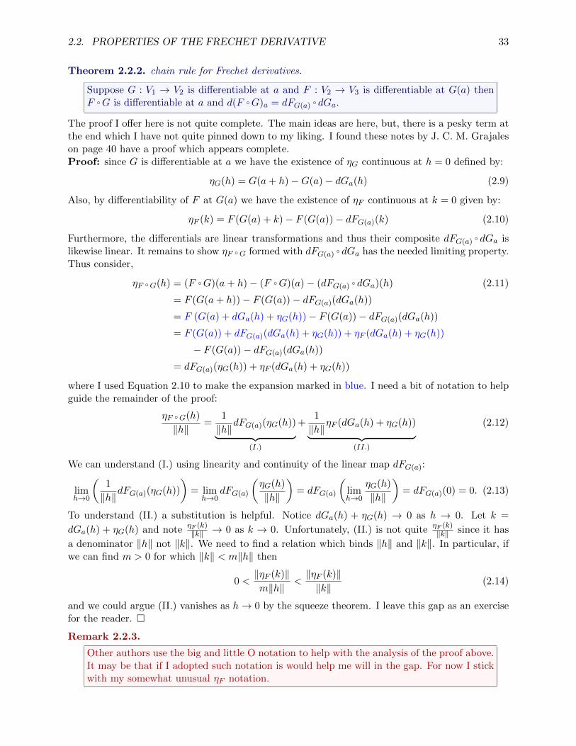
2.2. PROPERTIES OF THE FRECHET DERIVATIVE 33
Theorem 2.2.2. chain rule for Frechet derivatives.
Suppose G : V1 → V2 is differentiable at a and F : V2 → V3 is differentiable at G(a) thenF ◦G is differentiable at a and d(F ◦G)a = dFG(a) ◦ dGa.
The proof I offer here is not quite complete. The main ideas are here, but, there is a pesky term atthe end which I have not quite pinned down to my liking. I found these notes by J. C. M. Grajaleson page 40 have a proof which appears complete.Proof: since G is differentiable at a we have the existence of ηG continuous at h = 0 defined by:
ηG(h) = G(a+ h)−G(a)− dGa(h) (2.9)
Also, by differentiability of F at G(a) we have the existence of ηF continuous at k = 0 given by:
ηF (k) = F (G(a) + k)− F (G(a))− dFG(a)(k) (2.10)
Furthermore, the differentials are linear transformations and thus their composite dFG(a) ◦ dGa islikewise linear. It remains to show ηF ◦G formed with dFG(a) ◦ dGa has the needed limiting property.Thus consider,
ηF ◦G(h) = (F ◦G)(a+ h)− (F ◦G)(a)− (dFG(a) ◦ dGa)(h) (2.11)
= F (G(a+ h))− F (G(a))− dFG(a)(dGa(h))
= F (G(a) + dGa(h) + ηG(h))− F (G(a))− dFG(a)(dGa(h))
= F (G(a)) + dFG(a)(dGa(h) + ηG(h)) + ηF (dGa(h) + ηG(h))
− F (G(a))− dFG(a)(dGa(h))
= dFG(a)(ηG(h)) + ηF (dGa(h) + ηG(h))
where I used Equation 2.10 to make the expansion marked in blue. I need a bit of notation to helpguide the remainder of the proof:
ηF ◦G(h)
‖h‖=
1
‖h‖dFG(a)(ηG(h))︸ ︷︷ ︸
(I.)
+1
‖h‖ηF (dGa(h) + ηG(h))︸ ︷︷ ︸
(II.)
(2.12)
We can understand (I.) using linearity and continuity of the linear map dFG(a):
limh→0
(1
‖h‖dFG(a)(ηG(h))
)= lim
h→0dFG(a)
(ηG(h)
‖h‖
)= dFG(a)
(limh→0
ηG(h)
‖h‖
)= dFG(a)(0) = 0. (2.13)
To understand (II.) a substitution is helpful. Notice dGa(h) + ηG(h) → 0 as h → 0. Let k =
dGa(h) + ηG(h) and note ηF (k)‖k‖ → 0 as k → 0. Unfortunately, (II.) is not quite ηF (k)
‖k‖ since it has
a denominator ‖h‖ not ‖k‖. We need to find a relation which binds ‖h‖ and ‖k‖. In particular, ifwe can find m > 0 for which ‖k‖ < m‖h‖ then
0 <‖ηF (k)‖m‖h‖
<‖ηF (k)‖‖k‖
(2.14)
and we could argue (II.) vanishes as h→ 0 by the squeeze theorem. I leave this gap as an exercisefor the reader. �
Remark 2.2.3.
Other authors use the big and little O notation to help with the analysis of the proof above.It may be that if I adopted such notation is would help me will in the gap. For now I stickwith my somewhat unusual ηF notation.

34 CHAPTER 2. DIFFERENTIATION
2.3 partial derivatives of differentiable maps
In the preceding sections we calculated the differential at a point via educated guessing. We shouldlike to find better method to derive differentials. It turns out that we can systematically calculatethe differential from partial derivatives of the component functions. However, certain topologicalconditions are required for us to properly paste together the partial derivatives of the componentfunctions. We discuss the perils of constructing proving differentiability from partial derivatives inSection 2.4. The purpose of the current section is to define partial differentiation and to explainhow partial derivatives relate to the differential of a given differentiable map. To understand partialderivatives we begin with a study of directional derivatives. Once more we generalize the usualcalculus III.
Remark 2.3.1.
Certainly parts of what is done in this section naturally generalize to an infinite dimensionalcontext. You can read more about the Gateaux derivative in your future studies. However,here I limit our attention in this section to finite dimensional normed linear spaces.
2.3.1 partial differentiation in a finite dimensional real vector space
The directional derivative of a mapping F at a point a ∈ dom(F ) along v is defined to be thederivative of the curve γ(t) = F (a + tv). In other words, the directional derivative gives you theinstantaneous vector-rate of change in the mapping F at the point a along v.
Definition 2.3.2.
Suppose V and W are real normed linear spaces. Let F : dom(F ) ⊆ V → W and supposethe limit below exists for a ∈ dom(F ) and v ∈ V then we define the directional derivativeof F at a along v to be DvF (a) ∈W where
DvF (a) = limh→0
F (a+ hv)− F (a)
h
One great contrast we should pause to note is that the definition of the directional derivative isexplicit whereas the definition of the differential was implicit. Naturally, if we take V = W = Rthen we recover the first semester difference quotient definition of the derivative at a point. Thisalso reproduces the directional derivatives you were shown in multivariate calculus, except, we donot insist v have ‖v‖ = 1. Don’t be fooled by the proof of the next Theorem, it’s easier than itlooks. Summary: since differentiability at a point controls the change of the map in all directionsat a point in terms of the differential we can control the change in the map in a particular directionat the given point via the differential.
Theorem 2.3.3. Differentiability implies directional differentiability.
Let V,W be real normed linear spaces. If F : U ⊆ V → W is differentiable at a ∈ U thenthe directional derivative DvF (a) exists for each v ∈ V and DvF (a) = dFa(v).
Proof: Suppose a ∈ U such that dFa is well-defined then we are given that
limh→0
F (a+ h)− F (a)− dFa(h)
||h||= 0.

2.3. PARTIAL DERIVATIVES OF DIFFERENTIABLE MAPS 35
This is a limit in V , when it exists it follows that the limits that approach the origin along particularpaths also exist and are zero. Consider the path t 7→ tv for v 6= 0 and t > 0, we find
limtv→0, t>0
F (a+ tv)− F (a)− dFa(tv)
||tv||=
1
||v||limt→0+
F (a+ tv)− F (a)− tdFa(v)
|t|= 0.
Hence, as |t| = t for t > 0 we find
limt→0+
F (a+ tv)− F (a)
t= lim
t→0
tdFa(v)
t= dFa(v).
Likewise we can consider the path t 7→ tv for v 6= 0 and t < 0
limtv→0, t<0
F (a+ tv)− F (a)− dFa(tv)
||tv||=
1
||v||limt→0−
F (a+ tv)− F (a)− tdFa(v)
|t|= 0.
Note |t| = −t thus the limit above yields
limt→0−
F (a+ tv)− F (a)
−t= lim
t→0−
tdFa(v)
−t⇒ lim
t→0−
F (a+ tv)− F (a)
t= dFa(v).
Therefore,
limt→0
F (a+ tv)− F (a)
t= dFa(v)
and we conclude that DvF (a) = dFa(v) for all v ∈ V since the v = 0 case follows trivially. �
Partial derivatives are just directional derivatives in standard directions. In particular, given abasis β = {v1, . . . , vn} with coordinate maps x1, . . . , xn there is a standard concept of partialdifferentiation on an NLS:
Definition 2.3.4. partial derivative with respect to coordinate on an NLS.
Let V be a NLS with basis β = {v1, . . . , vn} and coordinates Φβ = (x1, . . . , xn). Then ifF : dom(F ) ⊆ V →W we define, for such points a ∈ dom(F ) as the limit exists,
∂F
∂xi(a) = DviF (a) = lim
h→0
F (a+ hvi)− F (a)
h.
Alternatively, we can present the partial derivative in terms of an ordinary derivative:
∂F
∂xi(a) =
d
dt[F (a+ tvi)]
∣∣∣∣t=0
(2.15)
Let’s revisit the map from Example 2.1.11 and see if we can recover the differential in terms ofpartial derivatives.
Example 2.3.5. Let F (X) = X2 for each X ∈ R n×n. Let Xij be the usual coordinates withrespect to the standard matrix basis {Eij}. Calculate the partial derivative of F with respect to Xij
at A: using Equation 2.15 with vi replaced with Eij and a with A,
∂F
∂Xij(A) =
d
dt
[(A+ tEij)
2] ∣∣∣∣t=0
(2.16)
=d
dt
[A2 + tAEij + tEijA+ t2E2
ij
] ∣∣∣∣t=0
= (AEij + EijA+ 2tE2ij)∣∣t=0
= AEij + EijA.

36 CHAPTER 2. DIFFERENTIATION
If we know a map of normed linear spaces is differentiable then we can express the differential interms of partial derivatives.
Theorem 2.3.6. differentials can be built from partial derivatives.
Let V,W be real normed linear spaces where V has basis β = {v1, . . . , vn} with coordinatesx1, . . . , xn. If F : dom(F ) ⊆ V →W is differentiable at a and h =
∑ni=1 hivi then
dFa(h) =n∑i=1
hi∂F
∂xi(a).
Proof: observe that
dFa
(n∑i=1
hivi
)=
n∑i=1
hidFa(vi) =
n∑i=1
hiDviF (a) =
n∑i=1
hi∂F
∂xi(a). (2.17)
follows immediately from linearity of differential paired with Theorem 2.3.3. �
Let’s apply the above result to Example 2.3.5.
Example 2.3.7. Consider F (X) = X2 for X ∈ R n×n. Construct the differential from the partialderivatives with respect to the standard basis matrix {Eij}. Let H =
∑i,j HijEij and calculate
using Equation 2.16
dFA(H) =∑i,j
Hij(AEij + EijA) = A
∑i,j
HijEij
+
∑i,j
HijEij
A = AH +HA.
I should emphasize, at this point in our development, we cannot conclude the differential existsmerely from partial derivatives existing6. The example above is reasonable because we have alreadyshown differentiability of the F (A) = A2 map in Example 2.1.11.
Remark 2.3.8.
I have deliberately defined the derivative in slightly more generality than we need for thiscourse. It’s probably not much trouble to continue to develop the theory of differentiationfor a normed vector space, however I will for the most part stop here modulo an examplehere or there. If you understand many of the theorems that follow from here on out forRn then it is a simple matter to transfer arguments to the setting of a Banach space byusing an appropriate isomorphism. Traditionally this type of course only covers continuousdifferentiability, inverse and implicit function theorems in the context of mappings fromRn to Rm.
For the reader interested in generalizing these results to the context of an abstract normedvector space feel free to discuss it with me sometime. Also, if you want to read a masteron these topics you could look at the text by Shlomo Sternberg on Advanced Calculus.He develops many things for normed spaces. Or, take a look at Dieudonne’s ModernAnalysis which pays special attention to reaping infinite dimensional results from our finite-dimensional arguments. I also find Zorich’s two volume set on Mathematical Analysis isquite helpful. I’m hoping to borrow some arguments from Zorich in this update to my notes.Any of these texts would be good to read to follow-up my course with something deeper.
6we study this in depth in Section 2.4.

2.3. PARTIAL DERIVATIVES OF DIFFERENTIABLE MAPS 37
2.3.2 partial differentiation for real
Consider F : dom(F ) ⊆ Rn → Rn, in this case the differential dFa is a linear transformationfrom Rn → Rn and we can calculate the standard matrix for the differential using the precedingproposition. Recall that if L : Rn → Rm then the standard matrix was simply
[L] = [L(e1)|L(e2)| · · · |L(en)]
and thus the action of L is expressed nicely as a matrix multiplication; L(v) = [L]v. Similarly,dFa : Rn → Rm is linear transformation and thus dFa(v) = [dFa]v where
[dFa] = [dFa(e1)|dFa(e2)| · · · |dFa(en)].
Moreover, by the preceding proposition we can calculate dFa(ej) = DejF (a) for j = 1, 2, . . . , n.Clearly the directional derivatives in the coordinate directions are of great importance. For thisreason we make the following definition:
Definition 2.3.9. Partial derivatives are directional derivatives in coordinate directions.
Suppose that F : U ⊆ Rn → Rm is a mapping the we say that F is has partial derivative∂F∂xi
(a) at a ∈ U iff the directional derivative in the ei direction exists at a. In this case wedenote,
∂F
∂xi(a) = DeiF (a).
Also, the notation DeiF (a) = DiF (a) or ∂iF = ∂F∂xi
is convenient. We construct the partialderivative function ∂iF : V ⊆ Rn → Rm as the function defined pointwise for each v ∈ Vwhere ∂iF (v) exists.
Let’s expand this definition a bit. Note that if F = (F1, F2, . . . , Fm) then
DeiF (a) = limh→0
F (a+ hei)− F (a)
h⇒ [DeiF (a)] · ej = lim
h→0
Fj(a+ hei)− Fj(a)
h
for each j = 1, 2, . . .m. But then the limit of the component function Fj is precisely the directionalderivative at a along ei hence we find the result
∂F
∂xi· ej =
∂Fj∂xi
in other words, ∂iF = (∂iF1, ∂iF2, . . . , ∂iFm).
In the particular case f : R2 → R the partial derivatives with respect to x and y at (xo, yo) arerelated to the graph z = f(x, y) as illustrated below:

38 CHAPTER 2. DIFFERENTIATION
Similar pictures can be imagined for partial derivatives of more variables, even for vector-valuedmaps, but direct visualization is not possible (at least for me).
The proposition below shows how the differential of a m-vector-valued function of n-real variablesis connected to a matrix of partial derivatives.
Proposition 2.3.10.
If F : U ⊆ Rn → Rm is differentiable at a ∈ U then the differential dFa has derivativematrix F ′(a) and it has components which are expressed in terms of partial derivatives ofthe component functions:
[dFa]ij = ∂jFi
for 1 ≤ i ≤ m and 1 ≤ j ≤ n.
Perhaps it is helpful to expand the derivative matrix explicitly for future reference:
F ′(a) =
∂1F1(a) ∂2F1(a) · · · ∂nF1(a)∂1F2(a) ∂2F2(a) · · · ∂nF2(a)
......
......
∂1Fm(a) ∂2Fm(a) · · · ∂nFm(a)
Let’s write the operation of the differential for a differentiable mapping at some point a ∈ R interms of the explicit matrix multiplication by F ′(a). Let v = (v1, v2, . . . vn) ∈ Rn,
dFa(v) = F ′(a)v =
∂1F1(a) ∂2F1(a) · · · ∂nF1(a)∂1F2(a) ∂2F2(a) · · · ∂nF2(a)
......
......
∂1Fm(a) ∂2Fm(a) · · · ∂nFm(a)
v1v2...vn
You may recall the notation from calculus III at this point, omitting the a-dependence,
∇Fj = grad(Fj) =[∂1Fj , ∂2Fj , · · · , ∂nFj
]TSo if the derivative exists we can write it in terms of a stack of gradient vectors of the componentfunctions: (I used a transpose to write the stack side-ways),
F ′ =[∇F1|∇F2| · · · |∇Fm
]TFinally, just to collect everything together,
F ′ =
∂1F1 ∂2F1 · · · ∂nF1
∂1F2 ∂2F2 · · · ∂nF2...
......
...∂1Fm ∂2Fm · · · ∂nFm
=[∂1F | ∂2F | · · · | ∂nF
]=
(∇F1)
T
(∇F2)T
...
(∇Fm)T
Example 2.3.11. Recall that in Example 2.1.6 we showed that F : R2 → R3 defined by F (x, y) =(xy, x2, x+ 3y) for all (x, y) ∈ R2 was differentiable. In fact we calculated that
dF(x,y)(h, k) =
y x2x 01 3
[ hk
].

2.3. PARTIAL DERIVATIVES OF DIFFERENTIABLE MAPS 39
If you recall from calculus III the mechanics of partial differentiation it’s simple to see that
∂F
∂x=
∂
∂x(xy, x2, x+ 3y) = (y, 2x, 1) =
y2x1
∂F
∂y=
∂
∂y(xy, x2, x+ 3y) = (x, 0, 3) =
x03
Thus [dF ] = [∂xF |∂yF ] (as we expect given the derivations in this section!)
Directional derivatives and partial derivatives are of secondary importance in this course. They aremerely the substructure of what is truly of interest: the differential. That said, it is useful to knowhow to construct directional derivatives via partial derivative formulas. In fact, in careless calculustexts it sometimes presented as the definition.
Proposition 2.3.12.
If F : U ⊆ Rn → Rm is differentiable at a ∈ U then the directional derivative DvF (a) canbe expressed as a sum of partial derivative maps for each v =< v1, v2, . . . , vn >∈ Rn:
DvF (a) =n∑j=1
vj∂jF (a)
Proof: since F is differentiable at a the differential dFa exists and DvF (a) = dFa(v) for all v ∈ Rn.Use linearity of the differential to calculate that
DvF (a) = dFa(v1e1 + · · ·+ vnen) = v1dFa(e1) + · · ·+ vndFa(en).
Note dFa(ej) = DejF (a) = ∂jF (a) and the prop. follows. �
Example 2.3.13. Suppose f : R3 → R then ∇f = [∂xf, ∂yf, ∂zf ]T and we can write the directionalderivative in terms of
Dvf = [∂xf, ∂yf, ∂zf ]T v = ∇f · vif we insist that ||v|| = 1 then we recover the standard directional derivative we discuss in calculusIII. Naturally the ||∇f(a)|| yields the maximum value for the directional derivative at a if we limitthe inputs to vectors of unit-length. If we did not limit the vectors to unit length then the directionalderivative at a can become arbitrarily large as Dvf(a) is proportional to the magnitude of v. Sinceour primary motivation in calculus III was describing rates of change along certain directions forsome multivariate function it made sense to specialize the directional derivative to vectors of unit-length. The definition used in these notes better serves the theoretical discussion.7
2.3.3 examples of Jacobian matrices
Our goal here is simply to exhibit the Jacobian matrix and partial derivatives for a few mappings.At the base of all these calculations is the observation that partial differentiation is just ordinarydifferentiation where we treat all the independent variable not being differentiated as constants.The criteria of independence is important. We’ll study the case where variables are not independentin a later section (see implicit differentiation).
7If you read my calculus III notes you’ll find a derivation of how the directional derivative in Stewart’s calculusarises from the general definition of the derivative as a linear mapping. Look up page 305g.

40 CHAPTER 2. DIFFERENTIATION
Example 2.3.14. Let f(t) = (t, t2, t3) then f ′(t) = (1, 2t, 3t2). In this case we have
f ′(t) = [dft] =
12t3t2
Example 2.3.15. Let f(~x, ~y) = ~x · ~y be a mapping from R3 ×R3 → R. I’ll denote the coordinatesin the domain by (x1, x2, x3, y1, y2, y3) thus f(~x, ~y) = x1y1 + x2y2 + x3y3. Calculate,
[df(~x,~y)] = ∇f(~x, ~y)T = [y1, y2, y3, x1, x2, x3]
Example 2.3.16. Let f(~x, ~y) = ~x · ~y be a mapping from Rn ×Rn → R. I’ll denote the coordinatesin the domain by (x1, . . . , xn, y1, . . . , yn) thus f(~x, ~y) =
∑ni=1 xiyi. Calculate,
∂xj
[ n∑i=1
xiyi
]=
n∑i=1
∂xixjyi =
n∑i=1
δijyi = yj
Likewise,
∂yj
[ n∑i=1
xiyi
]=
n∑i=1
xi∂yiyj
=n∑i=1
xiδij = xj
Therefore, noting that ∇f = (∂x1f, . . . , ∂xnf, ∂y1f, . . . , ∂ynf),
[df(~x,~y)]T = (∇f)(~x, ~y) = ~y × ~x = (y1, . . . , yn, x1, . . . , xn)
Example 2.3.17. Suppose F (x, y, z) = (xyz, y, z) we calculate,
∂F∂x = (yz, 0, 0) ∂F
∂y = (xz, 1, 0) ∂F∂z = (xy, 0, 1)
Remember these are actually column vectors in my sneaky notation; (v1, . . . , vn) = [v1, . . . , vn]T .This means the derivative or Jacobian matrix of F at (x, y, z) is
F ′(x, y, z) = [dF(x,y,z)] =
yz xz xy0 1 00 0 1
Example 2.3.18. Suppose F (x, y, z) = (x2 + z2, yz) we calculate,
∂F∂x = (2x, 0) ∂F
∂y = (0, z) ∂F∂z = (2z, y)
The derivative is a 2× 3 matrix in this example,
F ′(x, y, z) = [dF(x,y,z)] =
[2x 0 2z0 z y
]Example 2.3.19. Suppose F (x, y) = (x2 + y2, xy, x+ y) we calculate,
∂F∂x = (2x, y, 1) ∂F
∂y = (2y, x, 1)
The derivative is a 3× 2 matrix in this example,
F ′(x, y) = [dF(x,y)] =
2x 2yy x1 1
2.3. PARTIAL DERIVATIVES OF DIFFERENTIABLE MAPS 41
Example 2.3.20. Suppose P (x, v,m) = (Po, P1) = (12mv2 + 1
2kx2,mv) for some constant k. Let’s
calculate the derivative via gradients this time,
∇Po = (∂Po/∂x, ∂Po/∂v, ∂Po/∂m) = (kx,mv, 12v2)
∇P1 = (∂P1/∂x, ∂P1/∂v, ∂P1/∂m) = (0,m, v)
Therefore,
P ′(x, v,m) =
[kx mv 1
2v2
0 m v
]Example 2.3.21. Let F (r, θ) = (r cos θ, r sin θ). We calculate,
∂rF = (cos θ, sin θ) and ∂θF = (−r sin θ, r cos θ)
Hence,
F ′(r, θ) =
[cos θ −r sin θsin θ r cos θ
]Example 2.3.22. Let G(x, y) = (
√x2 + y2, tan−1(y/x)). We calculate,
∂xG =(
x√x2+y2
, −yx2+y2
)and ∂yG =
( y√x2+y2
, xx2+y2
)Hence,
G′(x, y) =
[x√x2+y2
y√x2+y2
−yx2+y2
xx2+y2
]=
[xr
yr−y
r2xr2
] (using r =
√x2 + y2
)Example 2.3.23. Let F (x, y) = (x, y,
√R2 − x2 − y2) for a constant R. We calculate,
∇√R2 − x2 − y2 =
(−x√
R2−x2−y2, −y√
R2−x2−y2
)Also, ∇x = (1, 0) and ∇y = (0, 1) thus
F ′(x, y) =
1 00 1−x√
R2−x2−y2−y√
R2−x2−y2
Example 2.3.24. Let F (x, y, z) = (x, y, z,
√R2 − x2 − y2 − z2) for a constant R. We calculate,
∇√R2 − x2 − y2 − z2 =
(−x√
R2−x2−y2−z2, −y√
R2−x2−y2−z2, −z√
R2−x2−y2−z2
)Also, ∇x = (1, 0, 0), ∇y = (0, 1, 0) and ∇z = (0, 0, 1) thus
F ′(x, y, z) =
1 0 00 1 00 0 1−x√
R2−x2−y2−z2−y√
R2−x2−y2−z2−z√
R2−x2−y2−z2

42 CHAPTER 2. DIFFERENTIATION
Example 2.3.25. Let f(x, y, z) = (x+ y, y + z, x+ z, xyz). You can calculate,
[df(x,y,z)] =
1 1 00 1 11 0 1yz xz xy
Example 2.3.26. Let f(x, y, z) = xyz. You can calculate,
[df(x,y,z)] =[yz xz xy
]Example 2.3.27. Let f(x, y, z) = (xyz, 1− x− y). You can calculate,
[df(x,y,z)] =
[yz xz xy−1 −1 0
]Example 2.3.28. Let f : R3 × R3 be defined by f(x) = x× v for a fixed vector v 6= 0. We denotex = (x1, x2, x3) and calculate,
∂
∂xa(x× v) =
∂
∂xa
( ∑i,j,k
εijkxivjek)
=∑i,j,k
εijk∂xi∂xa
vjek =∑i,j,k
εijkδiavjek =∑j,k
εajkvjek
It follows,∂
∂x1(x× v) =
∑j,k
ε1jkvjek = v2e3 − v3e2 = (0,−v3, v2)
∂
∂x2(x× v) =
∑j,k
ε2jkvjek = v3e1 − v1e3 = (v3, 0,−v1)
∂
∂x3(x× v) =
∑j,k
ε3jkvjek = v1e2 − v2e1 = (−v2, v1, 0)
Thus the Jacobian is simply,
[df(x,y)] =
0 v3 −v2−v3 0 −v1v2 v1 0
In fact, dfp(h) = f(h) = h × v for each p ∈ R3. The given mapping is linear so the differential ofthe mapping is precisely the mapping itself (we could short-cut much of this calculation and simplyquote Example 2.1.4 where we proved dT = T for linear T ).
Example 2.3.29. Let f(x, y) = (x, y, 1− x− y). You can calculate,
[df(x,y,z)] =
1 00 1−1 −1
Example 2.3.30. Let X(u, v) = (x, y, z) where x, y, z denote functions of u, v and I prefer to omitthe explicit depedendence to reduce clutter in the equations to follow.
∂X
∂u= Xu = (xu, yu, zu) and
∂X
∂v= Xv = (xv, yv, zv)
Then the Jacobian is the 3× 2 matrix
[dX(u,v)
]=
xu xvyu yvzu zv

2.3. PARTIAL DERIVATIVES OF DIFFERENTIABLE MAPS 43
Remark 2.3.31.
I return to these examples in the next chapter and we’ll explore the geometric content ofthese formulas as they support the application of certain theorems. More on that later, forthe remainder of this chapter we continue to focus on properties of differentiation.
2.3.4 on chain rule and Jacobian matrix multiplication
In calculus III you may have learned how to calculate partial derivatives in terms of tree-diagramsand intermediate variable etc... We now have a way of understanding those rules and all theother chain rules in terms of one over-arching calculation: matrix multiplication of the constituentJacobians in the composite function. Of course once we have this rule for the composite of twofunctions we can generalize to n-functions by a simple induction argument. For example, for threesuitably defined mappings F,G,H,
(F ◦G ◦H)′(a) = F ′(G(H(a)))G′(H(a))H ′(a)
Example 2.3.32. .
Example 2.3.33. .

44 CHAPTER 2. DIFFERENTIATION
Example 2.3.34. .
Example 2.3.35. .

2.4. CONTINUOUS DIFFERENTIABILITY 45
2.4 continuous differentiability
We have noted that differentiablility on some set U implies all sorts of nice formulas in terms ofthe partial derivatives. Curiously the converse is not quite so simple. It is possible for the partialderivatives to exist on some set and yet the mapping may fail to be differentiable. We need an extratopological condition on the partial derivatives if we are to avoid certain pathological8 examples.
Example 2.4.1. I found this example in Hubbard’s advanced calculus text(see Ex. 1.9.4, pg. 123).It is a source of endless odd examples, notation and bizarre quotes. Let f(x) = 0 and
f(x) =x
2+ x2 sin
1
x
for all x 6= 0. I can be shown that the derivative f ′(0) = 1/2. Moreover, we can show that f ′(x)exists for all x 6= 0, we can calculate:
f ′(x) =1
2+ 2x sin
1
x− cos
1
x
Notice that dom(f ′) = R. Note then that the tangent line at (0, 0) is y = x/2.
You might be tempted to say then that this function is increasing at a rate of 1/2 for x near zero.But this claim would be false since you can see that f ′(x) oscillates wildly without end near zero.We have a tangent line at (0, 0) with positive slope for a function which is not increasing at (0, 0)(recall that increasing is a concept we must define in a open interval to be careful). This sort ofthing cannot happen if the derivative is continuous near the point in question.
The one-dimensional case is really quite special, even though we had discontinuity of the derivativewe still had a well-defined tangent line to the point. However, many interesting theorems in calculusof one-variable require the function to be continuously differentiable near the point of interest. Forexample, to apply the 2nd-derivative test we need to find a point where the first derivative is zeroand the second derivative exists. We cannot hope to compute f ′′(xo) unless f ′ is continuous at xo.The next example is sick.
Example 2.4.2. Let us define f(0, 0) = 0 and
f(x, y) =x2y
x2 + y2
for all (x, y) 6= (0, 0) in R2. It can be shown that f is continuous at (0, 0). Moreover, sincef(x, 0) = f(0, y) = 0 for all x and all y it follows that f vanishes identically along the coordinateaxis. Thus the rate of change in the e1 or e2 directions is zero. We can calculate that
∂f
∂x=
2xy3
(x2 + y2)2and
∂f
∂y=x4 − x2y2
(x2 + y2)2
If you examine the plot of z = f(x, y) you can see why the tangent plane does not exist at (0, 0, 0).
8”pathological” as in, ”your clothes are so pathological, where’d you get them?”

46 CHAPTER 2. DIFFERENTIATION
Notice the sides of the box in the picture are parallel to the x and y axes so the path consideredbelow would fall on a diagonal slice of these boxes9. Consider the path to the origin t 7→ (t, t) givesfx(t, t) = 2t4/(t2 + t2)2 = 1/2 hence fx(x, y)→ 1/2 along the path t 7→ (t, t), but fx(0, 0) = 0 hencethe partial derivative fx is not continuous at (0, 0). In this example, the discontinuity of the partialderivatives makes the tangent plane fail to exist.
One might be tempted to suppose that if a function is continuous at a given point and if allthe possible directional derivatives exist then differentiability should follow. It turns out this isnot sufficient since continuity of the function does not imply some continuity along the partialderivatives. For example:
Example 2.4.3. Let us define f : R2 → R by f(x, y) = 0 for y 6= x2 and f(x, x2) = x. I invite thereader to verify that this function is continuous at the origin. Moreover, consider the directionalderivatives at (0, 0). We calculate, if v = 〈a, b〉
Dvf(0, 0) = limh→0
f(0 + hv)− f(0)
h= lim
h→0
f(ah, bh)
h= lim
h→0
0
h= 0.
To see why f(ah, bh) = 0, consider the intersection of ~r(h) = (ha, hb) and y = x2 the intersectionis found at hb = (ha)2 hence, noting h = 0 is not of interest in the limit, b = ha2. If a = 0then clearly (ah, bh) only falls on y = x2 at (0, 0). If a 6= 0 then the solution h = b/a2 givesf(ha, hb) = ha a nontrivial value. However, as h → 0 we eventually reach values close enoughto (0, 0) that f(ah, bh) = 0. Hence we find all directional derivatives exist and are zero at (0, 0).Let’s examine the graph of this example to see how this happened. The pictures below graph thexy-plane as red and the nontrivial values of f as a blue curve. The union of these forms the graphz = f(x, y).
9the argument to follow stands alone, you don’t need to understand the picture to understand the math here, butit’s nice if you do
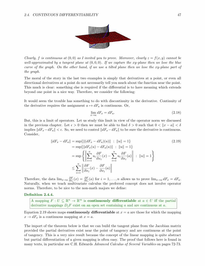
2.4. CONTINUOUS DIFFERENTIABILITY 47
Clearly, f is continuous at (0, 0) as I invited you to prove. Moreover, clearly z = f(x, y) cannot bewell-approximated by a tangent plane at (0, 0, 0). If we capture the xy-plane then we lose the bluecurve of the graph. On the other hand, if we use a tilted plane then we lose the xy-plane part ofthe graph.
The moral of the story in the last two examples is simply that derivatives at a point, or even alldirectional derivatives at a point do not necessarily tell you much about the function near the point.This much is clear: something else is required if the differential is to have meaning which extendsbeyond one point in a nice way. Therefore, we consider the following:
It would seem the trouble has something to do with discontinuity in the derivative. Continuity ofthe derivative requires the assignment a 7→ dFa is continuous. Or,
limx→a
dFx = dFa. (2.18)
But, this is a limit of operators. Let us study this limit in view of the operator norm we discussedin the previous chapter. Let ε > 0 then we must be able to find δ > 0 such that 0 < ‖x − a‖ < δimplies ‖dFx−dFa‖ < ε. So, we need to control ‖dFx−dFa‖ to be sure the derivative is continuous.Consider,
‖dFx − dFa‖ = sup{‖(dFx − dFa)(u)‖ : ‖u‖ = 1} (2.19)
= sup{‖dFx(u)− dFa(u)‖ : ‖u‖ = 1}
= sup
{∥∥∥∥∥n∑i=1
ui∂F
∂xi(x)−
n∑i=1
ui∂F
∂xi(a)
∥∥∥∥∥ : ‖u‖ = 1
}
≤n∑i=1
∥∥∥∥ ∂F∂xi (x)− ∂F
∂xi(a)
∥∥∥∥Therefore, the data limx→a
∂F∂xi
(x) = ∂F∂xi
(a) for i = 1, . . . , n allows us to prove limx→a dFx = dFa.Naturally, when we teach multivariate calculus the preferred concept does not involve operatornorms. Therefore, to be nice to the non-math majors we define:
Definition 2.4.4.
A mapping F : U ⊆ Rn → Rm is continuously differentiable at a ∈ U iff the partialderivative mappings DjF exist on an open set containing a and are continuous at a.
Equation 2.19 shows maps continuously differentiable at x = a are those for which the mappingx→ dFx is a continuous mapping at x = a.
The import of the theorem below is that we can build the tangent plane from the Jacobian matrixprovided the partial derivatives exist near the point of tangency and are continuous at the pointof tangency. This is a very nice result because the concept of the linear mapping is quite abstractbut partial differentiation of a given mapping is often easy. The proof that follows here is found inmany texts, in particular see C.H. Edwards Advanced Calculus of Several Variables on pages 72-73.

48 CHAPTER 2. DIFFERENTIATION
Theorem 2.4.5.
If F : Rn → R is continuously differentiable at a then F is differentiable at a
Proof: Consider a+h sufficiently close to a that all the partial derivatives of F exist. Furthermore,consider going from a to a+h by traversing a hyper-parallel-piped travelling n-perpendicular paths:
a︸︷︷︸po
→ a+ h1e1︸ ︷︷ ︸p1
→ a+ h1e1 + h2e2︸ ︷︷ ︸p2
→ · · · a+ h1e1 + · · ·+ hnen︸ ︷︷ ︸pn
= a+ h.
Let us denote pj = a+ bj where clearly bj ranges from bo = 0 to bn = h and bj =∑j
i=1 hiei. Noticethat the difference between pj and pj−1 is given by:
pj − pj−1 = a+
j∑i=1
hiei − a−j−1∑i=1
hiei = hjej
Consider then the following identity,
F (a+ h)− F (a) = F (pn)− F (pn−1) + F (pn−1)− F (pn−2) + · · ·+ F (p1)− F (po)
This is to say the change in F from po = a to pn = a+ h can be expressed as a sum of the changesalong the n-steps. Furthermore, if we consider the difference F (pj)−F (pj−1) you can see that onlythe j-th component of the argument of F changes. Since the j-th partial derivative exists on theinterval for hj considered by construction we can apply the mean value theorem to locate cj suchthat:
hj∂jF (pj−1 + cjej) = F (pj)− F (pj−1)
Therefore, using the mean value theorem for each interval, we select c1, . . . cn with:
F (a+ h)− F (a) =n∑j=1
hj∂jF (pj−1 + cjej)
It follows we should propose L to satisfy the definition of Frechet differentation as follows:
L(h) =
n∑j=1
hj∂jF (a)
It is clear that L is linear (in fact, perhaps you recognize this as L(h) = (∇F )(a) •h). Let usprepare to study the Frechet quotient,
F (a+ h)− F (a)− L(h) =n∑j=1
hj∂jF (pj−1 + cjej)−n∑j=1
hj∂jF (a)
=
n∑j=1
hj[∂jF (pj−1 + cjej)− ∂jF (a)︸ ︷︷ ︸
gj(h)
]Observe that pj−1+cjej → a as h→ 0. Thus, gj(h)→ 0 by the continuity of the partial derivativesat x = a. Finally, consider the Frechet quotient:
limh→0
F (a+ h)− F (a)− L(h)
||h||= lim
h→0
∑j hjgj(h)
||h||= lim
h→0
∑j
hj||h||
gj(h)
2.5. THE PRODUCT RULE 49
Notice |hj | ≤ ||h|| hence
∣∣∣∣ hj||h|| ∣∣∣∣ ≤ 1 and
0 ≤∣∣∣∣ hj||h||gj(h)
∣∣∣∣ ≤ |gj(h)|
Apply the squeeze theorem to deduce each term in the sum ? limits to zero. Consquently, L(h)satisfies the Frechet quotient and we have shown that F is differentiable at x = a and the differen-tial is expressed in terms of partial derivatives as expected; dFx(h) =
∑nj=1 hj∂jF (a) �.
Given the result above it is a simple matter to extend the proof to F : Rn → Rm.
Theorem 2.4.6.
If F : Rn → Rm is continuously differentiable at a then F is differentiable at a
Proof: If F is continuously differentiable at a then clearly each component function F j : Rn → Ris continuously differentiable at a. Thus, by Theorem 2.4.5 we have F j differentiable at a hence
limh→0
F j(a+ h)− F j(a)− dF ja (h)
||h||= 0 for all j ∈ Nm ⇒ lim
h→0
F (a+ h)− F (a)− dFa(h)
||h||= 0
by Theorem 1.3.11. This proves F is differentiable at a �.
2.5 the product rule
When I first wrote notes for advanced calculus I realized I was writing the same argument overand over. The result below is a result. This argument simultaneously covers derivatives of scalarmultiplications, matrix multiplications, dot and cross products.
Theorem 2.5.1.
Let W1,W2,W3, V be finite dimensional real normed linear spaces and suppose U ⊆ Vis open. Let β = {r1, . . . , rn} be a basis for V with coordinates x1, . . . , xn. Let γ1 ={w1, . . . , wm1} be the basis for W1. Let γ2 = {v1, . . . , vm2} be the basis for W2. Letγ3 = {ε1, . . . , εm3} be the basis for W3. Assume there exists a product ? : W1 ×W2 → W3
such that
(cx+ y) ? z = c(x ? z) + y ? z & x ? (cz + w) = c(x ? z) + x ? w
for all c ∈ R and x, y ∈ W1 and z, w ∈ W2. Then, if F : U → W1 and G : U → W2 arecontinuously differentiable at a ∈ U then F ?G is continuously differentiable at a ∈ U where(F ? G)(a) = F (a) ? G(a). Moreover, denoting ∂/∂xj by ∂j we have
∂j(F ? G)(a) = (∂jF )(a) ? G(a) + F (a) ? (∂jG)(a).
Hence, for each h ∈ V ,
d(F ? G)a(h) = dFa(h) ? G(a) + F (a) ? dGa(h).
50 CHAPTER 2. DIFFERENTIATION
Proof: assume the notation given in the Theorem and define structure constants cijk ∈ R suchthat:
vi ? wj =
m3∑k=1
cijkεk. (2.20)
These constants characterize the nature of the multiplication ?. Interestingly, they have little to dowith the proof, essentially the play the role of bystanders. Assuming F : U →W1 and G : U →W2
are continuously differentiable at a means their component functions F1, . . . , Fm1 : U → R withrespect to γ1 and G1, . . . , Gm2 : U → R with respect to γ2 are continuous at a. The componentfunctions of F ? G are naturally related to those of F and G as follows:
F ? G =
(m1∑i=1
Fivi
)?
m2∑j=1
Gjwj
(2.21)
=
m1∑i=1
m2∑j=1
FiGj (vi ? wj)
=
m1∑i=1
m2∑j=1
FiGj
(m3∑k=1
cijkεk
)
=
m3∑k=1
m1∑i=1
m2∑j=1
FiGjcijk
εk
Thus F ? G has component function∑m1
i=1
∑m2j=1 FiGjcijk. Observe this is the sum of products of
continuously differentiable functions at a which is once again continuously differentiable a. ThusF ? G is continuously differentiable at a as it has component functions whose partial derivativefunctions are continous at a. This becomes explicitly clear if we calculate the partial derivative ofF ? G with respect to xl for points near a,
∂l(F ? G) =
m3∑k=1
∂l
m1∑i=1
m2∑j=1
FiGjcijk
εk : ∂l done componentwise (2.22)
=
m3∑k=1
m1∑i=1
m2∑j=1
cijk∂l(FiGj)
εk : linearity of ∂l
=
m3∑k=1
m1∑i=1
m2∑j=1
cijk [(∂lFi)Gj + Fi∂lGj ]
εk : ordinary product rule
=
m1∑i=1
m2∑j=1
m3∑k=1
cijk(∂lFi)Gjεk +
m1∑i=1
m2∑j=1
m3∑k=1
cijkFi(∂lGj)εk
= (∂lF ) ? G+ F ? (∂lG).
where I used the calculation of Equation 2.21 in reverse in order to make the final step. Thecalculation makes it explicitly clear that the partial derivatives of F ? G are sums and products ofcontinuous functions hence F ?G is continuously differentiable as claimed. Finally, we can construct

2.5. THE PRODUCT RULE 51
the differential from partial derivatives: for h =∑n
l=1 hlrl calculate:
d(F ? G)a(h) =
n∑l=1
hl∂l(F ? G)(a) (2.23)
=
n∑l=1
hl [(∂lF )(a) ? G(a) + F (a) ? (∂lG)(a)]
=
[n∑l=1
hl(∂lF )(a)
]? G(a) + F (a) ?
[n∑l=1
hl(∂lG)(a)
].
= dFa(h) ? G(a) + F (a) ? dGa(h).
This completes the proof. �
Let’s unwrap a few common cases of this general product rule. I’ll continue to use the W1,W2,W3
and V notation to connect directly to Theorem 2.5.1.
(1.) Set W1 = W2 = W3 = R and V = R to produce the usual first semester calculusproduct rule:
d
dt(fg) =
df
dtg + f
dg
dt.
Of course, this was the heart of the proof.
(2.) Set W1 = W2 = W3 = R and V = Rn to produce the usual product rule forreal-valued functions of several variables:
∂
∂xi(fg) =
∂f
∂xig + f
∂g
∂xi.
(3.) Set W1 = R and W2 = W3 and V = Rn to produce the usual product rule for ascalar function multiplied on a vector-valued function:
∂
∂xi(f~v) =
∂f
∂xi~v + f
∂~v
∂xi.
(4.) Set W1 = W2 = Rn and W3 = R and V = R to produce the product rule fordot-products of paths:
d
dt(~v • ~w) =
d~v
dt• ~w + ~v •
d~w
dt.
(5.) Set W1 = W2 = R3 and W3 = R3 and V = R to produce the product rule forcross-products of paths:
d
dt(~v × ~w) =
d~v
dt× ~w + ~v × d~w
dt.
(6.) Set W1 = W2 = W3 = R n×n and V = R to produce the product rule for matrix-valued functions of a real variable: t 7→ A(t), t 7→ B(t),
d
dt(AB) =
dA
dtB +A
dB
dt.
(7.) Set W1 = W2 = W3 = C and V = C with z = x+ iy we find for f1 = u1 + iv1 andf2 = u2 + iv2
∂
∂x(f1f2) =
∂f1∂x
f2 + f1∂f2∂x
&∂
∂y(f1f2) =
∂f1∂y
f2 + f1∂f2∂y
.
52 CHAPTER 2. DIFFERENTIATION
Of course, there is much more. I simply wish to impress on you that these product rules are allsimply the standard product rule married to the algebraic structure of the given product. So longas the product has the needed linearity properties, there will be a corresponding product rule forfunctions.
2.6 higher derivatives
Given normed linear spaces V,W and U ⊆ V open and a differentiable map F : U → W we finda linear transformation dFa : V → W for each a ∈ U . Therefore, we can define the map f ′ : U →L(V ;W ) by the natural map a 7→ dFa. That is, f ′(a) = dfa. Furthermore, since L(V ;W ) is itselfa normed linear space we may study derivatives of f ′. In particular, if df ′a : V → L(V ;L(V ;W ))is linear for each a ∈ U and satisfies the needed Frechet quotient then we may likewise definef ′′ : U → L(V ;L(V ;W )) by f ′′(a) = (f ′)′(a) = (df ′)a ∈ L(V ;L(V ;W )) for each a ∈ U . This allgets a bit meta, so, its helpful to make use of an isomorphism Ψ : L(V ;L(V ;W )) → L(V, V ;W )defined by:
Ψ(T )(x, y) = (T (x))(y) (2.24)
for all x, y ∈ V and T ∈ L(V,W ). Typically the Ψ is not written. With this abuse of language, wehave f ′′(a) : V × V →W given by
f ′′(a)(h, k) = df ′a(h, k) = d(h 7→ dfh)a(k) (2.25)
Thus, in stark contrast to first semester calculus, each added derivative brings out a new object.Using the isomorphism and its extension to higher derivatives, we find the n-th derivative of f :V →W is naturally understood as an n-linear map from V to W . What is beautiful is that we cancapture this simply in terms of iterated partial derivatives provided a certain continuity is given.I’ll attempt to explain this for the case of second derivatives this semester. For the sake of time,I’ll let Zorich provide the many details I omit here. If I find time to prepare and Lecture, we mayexamine the proof that partial derivatives commute. Whether or not we have time for the proof,the fact that partial derivatives commute is a cornerstone of abstract calculus.
2.7 differentiation in an algebra variable
Here I share with you the rudiments of what I have come to call A-calculus. We say A is analgebra if there is a multiplication ? : A×A → A which behaves like ordinary multiplication:
(1.) (x+ y) ? z = x ? z + y ? z and x ? (y + z) = x ? y + x ? z
(2.) (cx) ? y = x ? (cy) = c(x ? y)
(3.) (x ? y) ? z = x ? (y ? z)
(4.) there exists 1A ∈ A for which 1A ? x = x = x ? 1A for each x ∈ A
I usually think about real algebras which means there is essentially a copy of R in the center ofthe algebra. In item (2.) I assume c ∈ R. However, the 1A may not appear manifestly as 1 ∈ R.Let me give a couple simple examples and forego the general theory.
Example 2.7.1. A = C is a nice example. If a + ib, c+ id ∈ C then we define (a + ib)(c+ id) =ac − bd + i(ad + bc). Equivalently, we could just proclaim i2 = −1 and otherwise, calculate likeusual. Here 1A = 1 as you might expect10
10Using C = R2 as a point set we note 1 = (1, 0) and i = (0, 1) hence c111 = 1 and c221 = −1 and c122 = c212 = 1whereas all other structure constants are zero. This has not much to do with anything, but, I thought it might befun given the proof of the previous section
2.7. DIFFERENTIATION IN AN ALGEBRA VARIABLE 53
Example 2.7.2. The direct product algebra of A = R×R is defined by (a, b)(x, y) = (ax, by).Here (1, 1)(x, y) = (x, y) for all (x, y) ∈ A and in fact 1A = (1, 1).
Example 2.7.3. The hyperbolic numbers are of the form a + bj where j2 = 1. In particular,define (a+ bj)(c+ jd) = ac+ bd+ j(ad+ bc).
Example 2.7.4. The 3-hyperbolic numbers are of the form a + bj + cj2 where j3 = 1. Inparticular, define
(a+ bj + cj2)(x+ jy + j2z) = ax+ by + cz + j(bx+ ay + cz) + j2(cx+ by + az).
All the algebras I’ve listed thus far are commutative. There are also many noncommutativealgebras like the quaternions or matrix algebras. Notice R n×n forms an algebra. Basically, I thinkof algebras as generalized number systems. So, given that, it is interesting to ask what it meansto differentiate with respect to a variable which takes values in A. In fact, we have a whole coursedevoted to studying what happens when you do calculus with respect to a complex variable. Manyschools have such a course. What is less known, which is a shame since it’s really pretty simple, isthat you can differentiate with respect to an algebra variable in much the same way.
Definition 2.7.5. Let U ⊆ A be an open set containing p. If f : U → A is a function then we sayf is A-differentiable at p if there exists a linear function dpf ∈ RA such that
limh→0
f(p+ h)− f(p)− dpf(h)
||h||= 0. (2.26)
When I say dpf ∈ RA this simply means that dpf : A → A is R-linear mapping on A and dpf(v ?w) = dpf(v) ? w for all v, w ∈ A. In other words, A-differentiability amounts to differentiability atp with an extra condition. Furthermore, we define the derivative at p as follows:
(dpf)(h) = f ′(p)h (2.27)
But, since (dpf)(h) = dpf(1 ? h) = dpf(1) ? h = f ′(p)h we have f ′(p) = dpf(1). In contrast tothe differential of an arbitrary real differentiable map on A, the formula for dpf is equivalent tothe selection of a number in A for p. In other words, there is a natural manner to interpret thederivative of a function as a function once more. Furthermore, it can be shown for higher derivativesof an A-differentiable function we have
dnf(v1, v2, . . . , vn) = dnf(1, 1, . . . , 1) ? v1 ? v2 ? · · · ? vn (2.28)
So the n-th derivative is also uniquely fixed by the value of dnf(1, 1, . . . , 1). In fact, we can naturallyidentify the n-th derivative of a function as a function once more. In general, the n-th derivative isa symmetric n-linear functon. Finally, I must tell you a beautiful formula which makes A-Calculusso very interesting: provided the basis for A has 1A = 1 paired with coordinate x1:
∂nf
∂xi1∂xi2 · · · ∂xin=∂nf
∂xn1? vi1 ? vi2 ? · · · ? vin (2.29)
If A = Rn as a point set and e1 = 1 then the formulas describing A-calculus are quite nice.
Example 2.7.6. Consider f = u + iv which is complex differentiable at p ∈ C. Use z = x + iyas the typical variable in C. Notice, dpf(i) = dpf(1)i implies that ∂f
∂y = ∂f∂x i. These are the famed
Cauchy Riemann equations. To help the reader make the connection, note fy = uy + ivy andfx = ux + ivx hence fy = ifx amounts to (uy + ivy) = i(ux + ivx) hence uy = −vx and vy = ux.Jumping ahead a bit, with no intention of explaining why here, it is fun to note since i2 + 1 = 0it follows fyy + fxx = 0 hence the component functions of a complex differentiable function aresolutions to Laplace’s equation.

54 CHAPTER 2. DIFFERENTIATION
Example 2.7.7. Consider f = u + jv which is hyperbolic differentiable at p ∈ H = R ⊕ jR(this is just notation for the hyperbolic numbers). Use z = x + jy as the typical variable in H.Notice, dpf(j) = dpf(1)j implies that ∂f
∂y = ∂f∂xj. These are the no so well-known hyperbolic Cauchy
Riemann equations. To help the reader make the connection, note fy = uy + jvy and fx = ux + jvxhence fy = jfx amounts to (uy + jvy) = j(ux + jvx) hence uy = vx and vy = ux. Jumpingahead a bit, with no intention of explaining why here, it is fun to note since 1 − j2 = 0 it followsfxx− fyy = 0 hence the component functions of a hyperbolic differentiable function are solutions tothe one-dimensional wave equation.
Basically, any identity which appears amongst the basis elements of an algebra will be mirrored ina PDE which is solve by each function differentiable over the algebra. Most familar case is with Cwhere harmonic functions are a standard and beatiful topic. But, this is just one of many functiontheories. In ordinary real analysis essentially A = R itself so this feature cannot be seen. However,once A is two or more dimensional, the differentiability with respect to A binds real variablestogether in such a way that the change in one real variable is necessarily coupled to the rest.
Ok, so, let’s return to our uber product rule once more, assume f, g are A-differentiable at p in acommutative algebra then note:
dp(f ? g)(v ? w) = (dpf)(v ? w) ? g(p) + f(p) ? dpg(v ? w) (2.30)
= dpf(v) ? w ? g(p) + f(p) ? dpg(v) ? w
= (dpf(v) ? g(p) + f(p) ? dpg(v)) ? w
We can argue f ? g is real differentiable and dp(f ? g) ∈ RA thus f ? g is A-differentiable at p.Moreover, as (f ? g)′(p) = dp(f ? g)(1) we derive from the result above that
(f ? g)′(p) = f ′(p) ? g(p) + f(p) ? g′(p).
Many further results about the calculus over an algebra are known and many resemble closelythe calculus you’ve already seen. However, I’ve also found a few suprises, mostly thanks to thestudents who’ve helped me study A-calculus the past few years. If this section was a bit too terse,my apologies, I have much more to say in my primer on A-calculus: Introduction to A-Calculusand my A-Calculus II paper with Daniel Freese and my differential equations on an algebra paperwith Nathan BeDell. I will probably share some tidbits about these papers when the time seemsright in this course. But, our main focus is elsewhere.
Chapter 3
inverse and implicit function theorems
It is tempting to give a complete and rigourous proof of these theorems at the outset, but I willresist the temptation in lecture. I’m actually more interested that the student understand what thetheorem claims before I show the real proof. I will sketch the proof and show many applications.A nearly complete proof is found in Edwards where he uses an iterative approximation techniquefounded on the contraction mapping principle, we will go through that a bit later in the course. Iprobably will not have typed notes on that material this semester, but Edward’s is fairly readableand I think we’ll profit from working through those sections. That said, we develop an intuition forjust what these theorems are all about to start. That is the point of this chapter: to grasp whatthe linear algebra of the Jacobian suggests about the local behaviour of functions and equations.
3.1 inverse function theorem
Consider the problem of finding a local inverse for f : dom(f) ⊆ R → R. If we are given a pointp ∈ dom(f) such that there exists an open interval I containing p with f |I a one-one function thenwe can reasonably construct an inverse function by the simple rule f−1(y) = x iff f(x) = y forx ∈ I and y ∈ f(I). A sufficient condition to insure the existence of a local inverse is that thederivative function is either strictly positive or strictly negative on some neighborhood of p. If weare give a continuously differentiable function at p then it has a derivative which is continuous onsome neighborhood of p. For such a function if f ′(p) 6= 0 then there exists some interval centered atp for which the derivative is strictly positive or negative. It follows that such a function is strictlymonotonic and is hence one-one thus there is a local inverse at p. We should all learn in calculusI that the derivative informs us about the local invertibility of a function. Natural question to askfor us here: does this extend to higher dimensions? If so, how?
The arguments I just made are supported by theorems that are developed in calculus I. Let me shiftgears a bit and give a direct calculational explaination based on the linearization approximation.
If x ≈ p then f(x) ≈ f(p) + f ′(p)(x− p). To find the formula for the inverse we solve y = f(x) forx:
y ≈ f(p) + f ′(p)(x− p) ⇒ x ≈ p+1
f ′(p)
[y − f(p)
]Therefore, f−1(y) ≈ p+
1
f ′(p)
[y − f(p)
]for y near f(p).
55

56 CHAPTER 3. INVERSE AND IMPLICIT FUNCTION THEOREMS
Example 3.1.1. Just to help you believe me, consider f(x) = 3x − 2 then f ′(x) = 3 for all x.Suppose we want to find the inverse function near p = 2 then the discussion preceding this examplesuggests,
f−1(y) = 2 +1
3(y − 4).
I invite the reader to check that f(f−1(y)) = y and f−1(f(x)) = x for all x, y ∈ R.
In the example above we found a global inverse exactly, but this is thanks to the linearity of thefunction in the example. Generally, inverting the linearization just gives the first approximation tothe inverse.
Consider F : dom(F ) ⊆ Rn → Rn. If F is differentiable at p ∈ Rn then we can write F (x) ≈F (p) +F ′(p)(x− p) for x ≈ p. Set y = F (x) and solve for x via matrix algebra. This time we needto assume F ′(p) is an invertible matrix in order to isolate x,
y ≈ F (p) + F ′(p)(x− p) ⇒ x ≈ p+ (F ′(p))−1[y − f(p)
]Therefore,
F−1(y) ≈ p+ (F ′(p))−1[y − f(p)
]for y near F (p). Apparently the condition to find a local inverse for a mapping on Rn is that thederivative matrix is nonsingular1 in some neighborhood of the point. Experience has taught usfrom the one-dimensional case that we must insist the derivative is continuous near the point inorder to maintain the validity of the approximation.
Recall from calculus II that as we attempt to approximate a function with a power series it takesan infinite series of power functions to recapture the formula exactly. Well, something similar istrue here. However, the method of approximation is through an iterative approximation procedurewhich is built off the idea of Newton’s method. The product of this iteration is a nested sequenceof composite functions. To prove the theorem below one must actually provide proof the recur-sively generated sequence of functions converges. See pages 160-187 of Edwards for an in-depthexposition of the iterative approximation procedure. Then see pages 404-411 of Edwards for somematerial on uniform convergence2 The main analytical tool which is used to prove the convergenceis called the contraction mapping principle. The proof of the principle is relatively easy tofollow and interestingly the main non-trivial step is an application of the geometric series. Forthe student of analysis this is an important topic which you should spend considerable time reallytrying to absorb as deeply as possible. The contraction mapping is at the base of a number ofinteresting and nontrivial theorems. Read Rosenlicht’s Introduction to Analysis for a broader andbetter organized exposition of this analysis. In contrast, Edwards’ uses analysis as a tool to obtainresults for advanced calculus but his central goal is not a broad or well-framed treatment of analysis.Consequently, if analysis is your interest then you really need to read something else in parallel toget a better ideas about sequences of functions and uniform convergence. I have some notes froma series of conversations with a student about Rosenlicht, I’ll post those for the interested student.These notes focus on the part of the material I require for this course. This is Theorem 3.3 on page185 of Edwards’ text:
1nonsingular matrices are also called invertible matrices and a convenient test is that A is invertible iff det(A) 6= 0.2actually that later chapter is part of why I chose Edwards’ text, he makes a point of proving things in Rn in such
a way that the proof naturally generalizes to function space. This is done by arguing with properties rather thanformulas. The properties offen extend to infinite dimensions whereas the formulas usually do not.

3.1. INVERSE FUNCTION THEOREM 57
Theorem 3.1.2. ( inverse function theorem )
Suppose F : Rn → Rn is continuously differentiable in an open set W containing a and thederivative matrix F ′(a) is invertible. Then F is locally invertible at a. This means thatthere exists an open set U ⊆ W containing a and V a open set containing b = F (a) anda one-one, continuously differentiable mapping G : V → W such that G(F (x)) = x for allx ∈ U and F (G(y)) = y for all y ∈ V . Moreover, the local inverse G can be obtained as thelimit of the sequence of successive approximations defined by
Go(y) = a and Gn+1(y) = Gn(y)− [F ′(a)]−1[F (Gn(y))− y] for all y ∈ V .
The qualifier local is important to note. If we seek a global inverse then other ideas are needed.If the function is everywhere injective then logically F (x) = y defines F−1(y) = x and F−1 soconstructed in single-valued by virtue of the injectivity of F . However, for differentiable mappings,one might wonder how can the criteria of global injectivity be tested via the differential. Even inthe one-dimensional case a vanishing derivative does not indicate a lack of injectivity; f(x) = x3
has f−1(y) = 3√y and yet f ′(0) = 0 (therefore f ′(0) is not invertible). One the other hand, we’ll see
in the examples that follow that even if the derivative is invertible over a set it is possible for thevalues of the mapping to double-up and once that happens we cannot find a single-valued inversefunction3
Remark 3.1.3. James R. Munkres’ Analysis on Manifolds good for a different proof.
Another good place to read the inverse function theorem is in James R. Munkres Analysison Manifolds. That text is careful and has rather complete arguments which are not entirelythe same as the ones given in Edwards. Munkres’ text does not use the contraction mappingprinciple, instead the arguments are more topological in nature.
To give some idea of what I mean by topological let be give an example of such an argument.Suppose F : Rn → Rn is continuously differentiable and F ′(p) is invertible. Here’s a sketch of theargument that F ′(x) is invertible for all x near p as follows:
1. the function g : Rn → R defined by g(x) = det(F ′(x)) is formed by a multinomial in thecomponent functions of F ′(x). This function is clearly continuous since we are given that thepartial derivatives of the component functions of F are all continuous.
2. note we are given F ′(p) is invertible and hence det(F ′(p)) 6= 0 thus the continuous function gis nonzero at p. It follows there is some open set U containing p for which 0 /∈ g(U)
3. we have det(F ′(x)) 6= 0 for all x ∈ U hence F ′(x) is invertible on U .
I would argue this is a topological argument because the key idea here is the continuity of g.Topology is the study of continuity in general.
Remark 3.1.4. James J. Callahan’s Advanced Calculus: a Geometric View, good reading.
James J. Callahan’s Advanced Calculus: a Geometric View has great merit in both visual-ization and well-thought use of linear algebraic techniques. In addition, many student willenjoy his staggered proofs where he first shows the proof for a simple low dimensional caseand then proceeds to the general case.
3there are scientists and engineers who work with multiply-valued functions with great success, however, as a pointof style if nothing else, we try to use functions in math.

58 CHAPTER 3. INVERSE AND IMPLICIT FUNCTION THEOREMS
Example 3.1.5. Suppose F (x, y) =(
sin(y) + 1, sin(x) + 2)
for (x, y) ∈ R2. Clearly F is contin-uously differentiable as all its component functions have continuous partial derivatives. Observe,
F ′(x, y) = [ ∂xF | ∂yF ] =
[0 cos(y)
cos(x) 0
]Hence F ′(x, y) is invertible at points (x, y) such that det(F ′(x, y)) = − cos(x) cos(y) 6= 0. Thismeans we may not be able to find local inverses at points (x, y) with x = 1
2(2n + 1)π or y =12(2m + 1)π for some m,n ∈ Z. Points where F ′(x, y) are singular are points where one or bothof sin(y) and sin(x) reach extreme values thus the points where the Jacobian matrix are singularare in fact points where we cannot find a local inverse. Why? Because the function is clearly not1-1 on any set which contains the points of singularity for dF . Continuing, recall from precalculusthat sine has a standard inverse on [−π/2, π/2]. Suppose (x, y) ∈ [−π/2, π/2]2 and seek to solveF (x, y) = (a, b) for (x, y):
F (x, y) =
[sin(y) + 1sin(x) + 2
]=
[ab
]⇒
{sin(y) + 1 = asin(x) + 2 = b
}⇒
{y = sin−1(a− 1)x = sin−1(b− 2)
}It follows that F−1(a, b) =
(sin−1(b − 2), sin−1(a − 1)
)for (a, b) ∈ [0, 2] × [1, 3] where you should
note F ([−π/2, π/2]2) = [0, 2]× [1, 3]. We’ve found a local inverse for F on the region [−π/2, π/2]2.In other words, we just found a global inverse for the restriction of F to [−π/2, π/2]2. Technicallywe ought not write F−1, to be more precise we should write:
(F |[−π/2,π/2]2)−1(a, b) =(sin−1(b− 2), sin−1(a− 1)
).
It is customary to avoid such detail in many contexts. Inverse functions for sine, cosine, tangentetc... are good examples of this slight of langauge.
A coordinate system on Rn is an invertible mapping of Rn to Rn. However, in practice the termcoordinate system is used with less rigor. Often a coordinate system has various degeneracies. Forexample, in polar coordinates you could say θ = π/4 or θ = 9π/4 or generally θ = 2πk + π/4 forany k ∈ Z. Let’s examine polar coordinates in view of the inverse function theorem.
Example 3.1.6. Let T (r, θ) =(r cos(θ), r sin(θ)
)for (r, θ) ∈ [0,∞) × (−π/2, π/2). Clearly
T is continuously differentiable as all its component functions have continuous partial derivatives.To find the inverse we seek to solve T (r, θ) = (x, y) for (r, θ). Hence, consider x = r cos(θ) andy = r sin(θ). Note that
x2 + y2 = r2 cos2(θ) + r2 sin2(θ) = r2(cos2(θ) + sin2(θ)) = r2
andy
x=r sin(θ)
r cos(θ)= tan(θ).
It follows that r =√x2 + y2 and θ = tan−1(y/x) for (x, y) ∈ (0,∞)× R. We find
T−1(x, y) =
( √x2 + y2, tan−1(y/x)
).
Let’s see how the derivative fits with our results. Calcuate,
T ′(r, θ) = [ ∂rT | ∂θT ] =
[cos(θ) −r sin(θ)sin(θ) r cos(θ)
]

3.2. IMPLICIT FUNCTION THEOREM 59
note that det(T ′(r, θ)) = r hence we the inverse function theorem provides the existence of a localinverse around any point except the origin. Notice the derivative does not detect the defect in theangular coordinate. Challenge, find the inverse function for T (r, θ) =
(r cos(θ), r sin(θ)
)with
dom(T ) = [0,∞) × (π/2, 3π/2). Or, find the inverse for polar coordinates in a neighborhood of(0,−1).
Example 3.1.7. Suppose T : R3 → R3 is defined by T (x, y, z) = (ax, by, cz) for constants a, b, c ∈R where abc 6= 0. Clearly T is continuously differentiable as all its component functions havecontinuous partial derivatives. We calculate T ′(x, y, z) = [∂xT |∂yT |∂zT ] = [ae1|be2|ce3]. Thusdet(T ′(x, y, z)) = abc 6= 0 for all (x, y, z) ∈ R3 hence this function is locally invertible everywhere.Moreover, we calculate the inverse mapping by solving T (x, y, z) = (u, v, w) for (x, y, z):
(ax, by, cz) = (u, v, w) ⇒ (x, y, z) = (u/a, v/b, w/c) ⇒ T−1(u, v, w) = (u/a, v/b, w/c).
Example 3.1.8. Suppose F : Rn → Rn is defined by F (x) = Ax+b for some matrix A ∈ R n×n andvector b ∈ Rn. Under what conditions is such a function invertible ?. Since the formula forthis function gives each component function as a polynomial in the n-variables we can conclude thefunction is continuously differentiable. You can calculate that F ′(x) = A. It follows that a sufficientcondition for local inversion is det(A) 6= 0. It turns out that this is also a necessary condition asdet(A) = 0 implies the matrix A has nontrivial solutions for Av = 0. We say v ∈ Null(A) iffAv = 0. Note if v ∈ Null(A) then F (v) = Av + b = b. This is not a problem when det(A) 6= 0for in that case the null space is contains just zero; Null(A) = {0}. However, when det(A) = 0 welearn in linear algebra that Null(A) contains infinitely many vectors so F is far from injective. Forexample, suppose Null(A) = span{e1} then you can show that F (a1, a2, . . . , an) = F (x, a2, . . . , an)for all x ∈ R. Hence any point will have other points nearby which output the same value under F .Suppose det(A) 6= 0, to calculate the inverse mapping formula we should solve F (x) = y for x,
y = Ax+ b ⇒ x = A−1(y − b) ⇒ F−1(y) = A−1(y − b).
Remark 3.1.9. inverse function theorem holds for higher derivatives.
In Munkres the inverse function theorem is given for r-times differentiable functions. Inshort, a Cr function with invertible differential at a point has a Cr inverse function localto the point. Edwards also has arguments for r > 1, see page 202 and arguments andsurrounding arguments.
3.2 implicit function theorem
Consider the problem of solving x2 + y2 = 1 for y as a function of x.
x2 + y2 = 1 ⇒ y2 = 1− x2 ⇒ y = ±√
1− x2.
A function cannot have two outputs for a single input, when we write ± in the expression aboveit simply indicates our ignorance as to which is chosen. Once further information is given then wemay be able to choose a + or a −. For example:
1. if x2 + y2 = 1 and we want to solve for y near (0, 1) then y =√
1− x2 is the correct choicesince y > 0 at the point of interest.

60 CHAPTER 3. INVERSE AND IMPLICIT FUNCTION THEOREMS
2. if x2 +y2 = 1 and we want to solve for y near (0,−1) then y = −√
1− x2 is the correct choicesince y < 0 at the point of interest.
3. if x2 + y2 = 1 and we want to solve for y near (1, 0) then it’s impossible to find a singlefunction which reproduces x2 + y2 = 1 on an open disk centered at (1, 0).
What is the defect of case (3.) ? The trouble is that no matter how close we zoom in to the pointthere are always two y-values for each given x-value. Geometrically, this suggests either we have adiscontinuity, a kink, or a vertical tangent in the graph. The given problem has a vertical tangentand hopefully you can picture this with ease since its just the unit-circle. In calculus I we studiedimplicit differentiation, our starting point was to assume y = y(x) and then we differentiatedequations to work out implicit formulas for dy/dx. Take the unit-circle and differentiate both sides,
x2 + y2 = 1 ⇒ 2x+ 2ydy
dx= 0 ⇒ dy
dx= −x
y.
Note dydx is not defined for y = 0. It’s no accident that those two points (−1, 0) and (1, 0) are
precisely the points at which we cannot solve for y as a function of x. Apparently, the singularityin the derivative indicates where we may have trouble solving an equation for one variable as afunction of the remaining variable.
We wish to study this problem in general. Given n-equations in (m+n)-unknowns when can we solvefor the last n-variables as functions of the first m-variables ? Given a continuously differentiablemapping G = (G1, G2, . . . , Gn) : Rm × Rn → Rn study the level set: (here k1, k2, . . . , kn areconstants)
G1(x1, . . . , xm, y1, . . . , yn) = k1
G2(x1, . . . , xm, y1, . . . , yn) = k2...
Gn(x1, . . . , xm, y1, . . . , yn) = kn
We wish to locally solve for y1, . . . , yn as functions of x1, . . . xm. That is, find a mapping h : Rm →Rn such that G(x, y) = k iff y = h(x) near some point (a, b) ∈ Rm × Rn such that G(a, b) = k. Inthis section we use the notation x = (x1, x2, . . . xm) and y = (y1, y2, . . . , yn).
Before we turn to the general problem let’s analyze the unit-circle problem in this notation. Weare given G(x, y) = x2 + y2 and we wish to find f(x) such that y = f(x) solves G(x, y) = 1.Differentiate with respect to x and use the chain-rule:
∂G
∂x
dx
dx+∂G
∂y
dy
dx= 0
We find that dy/dx = −Gx/Gy = −x/y. Given this analysis we should suspect that if we are
given some level curve G(x, y) = k then we may be able to solve for y as a function of x near pif G(p) = k and Gy(p) 6= 0. This suspicion is valid and it is one of the many consequences of theimplicit function theorem.
We again turn to the linearization approximation. Suppose G(x, y) = k where x ∈ Rm and y ∈ Rnand suppose G : Rm × Rn → Rn is continuously differentiable. Suppose (a, b) ∈ Rm × Rn hasG(a, b) = k. Replace G with its linearization based at (a, b):
G(x, y) ≈ k +G′(a, b)(x− a, y − b)
3.2. IMPLICIT FUNCTION THEOREM 61
here we have the matrix multiplication of the n × (m + n) matrix G′(a, b) with the (m + n) × 1column vector (x − a, y − b) to yield an n-component column vector. It is convenient to definepartial derivatives with respect to a whole vector of variables,
∂G
∂x=
∂G1∂x1
· · · ∂G1∂xm
......
∂Gn∂x1
· · · ∂Gn∂xm
∂G
∂y=
∂G1∂y1
· · · ∂G1∂yn
......
∂Gn∂y1
· · · ∂Gn∂yn
In this notation we can write the n × (m + n) matrix G′(a, b) as the concatenation of the n ×mmatrix ∂G
∂x (a, b) and the n× n matrix ∂G∂y (a, b)
G′(a, b) =
[∂G
∂x(a, b)
∣∣∣∣∂G∂y (a, b)
]Therefore, for points close to (a, b) we have:
G(x, y) ≈ k +∂G
∂x(a, b)(x− a) +
∂G
∂y(a, b)(y − b)
The nonlinear problem G(x, y) = k has been (locally) replaced by the linear problem of solvingwhat follows for y:
k ≈ k +∂G
∂x(a, b)(x− a) +
∂G
∂y(a, b)(y − b) (3.1)
Suppose the square matrix ∂G∂y (a, b) is invertible at (a, b) then we find the following approximation
for the implicit solution of G(x, y) = k for y as a function of x:
y = b−[∂G
∂y(a, b)
]−1[∂G∂x
(a, b)(x− a)
].
Of course this is not a formal proof, but it does suggest that det[∂G∂y (a, b)
]6= 0 is a necessary
condition for solving for the y variables.
As before suppose G : Rm × Rn → Rn. Suppose we have a continuously differentiable functionh : Rm → Rn such that h(a) = b and G(x, h(x)) = k. We seek to find the derivative of h in termsof the derivative of G. This is a generalization of the implicit differentiation calculation we performin calculus I. I’m including this to help you understand the notation a bit more before I state theimplicit function theorem. Differentiate with respect to xl for l ∈ Nm:
∂
∂xl
[G(x, h(x))
]=
m∑i=1
∂G
∂xi
∂xi∂xl
+
n∑j=1
∂G
∂yj
∂hj∂xl
=∂G
∂xl+
n∑j=1
∂G
∂yj
∂hj∂xl
= 0
we made use of the identity ∂xi∂xk
= δik to squash the sum of i to the single nontrivial term and the
zero on the r.h.s follows from the fact that ∂∂xl
(k) = 0. Concatenate these derivatives from k = 1up to k = m:[
∂G
∂x1+
n∑j=1
∂G
∂yj
∂hj∂x1
∣∣∣∣ ∂G∂x2 +
n∑j=1
∂G
∂yj
∂hj∂x2
∣∣∣∣ · · · ∣∣∣∣ ∂G∂xm +
n∑j=1
∂G
∂yj
∂hj∂xm
]= [0|0| · · · |0]
Properties of matrix addition allow us to parse the expression above as follows:[∂G
∂x1
∣∣∣∣ ∂G∂x2∣∣∣∣ · · · ∣∣∣∣ ∂G∂xm
]+
[ n∑j=1
∂G
∂yj
∂hj∂x1
∣∣∣∣ n∑j=1
∂G
∂yj
∂hj∂x2
∣∣∣∣ · · · ∣∣∣∣ n∑j=1
∂G
∂yj
∂hj∂xm
]= [0|0| · · · |0]

62 CHAPTER 3. INVERSE AND IMPLICIT FUNCTION THEOREMS
But, this reduces to
∂G
∂x+
[∂G
∂y
∂h
∂x1
∣∣∣∣∂G∂y ∂h
∂x2
∣∣∣∣ · · · ∣∣∣∣∂G∂y ∂h
∂xm
]= 0 ∈ Rm×n
The concatenation property of matrix multiplication states [Ab1|Ab2| · · · |Abm] = A[b1|b2| · · · |bm]we use this to write the expression once more,
∂G
∂x+∂G
∂y
[∂h
∂x1
∣∣∣∣ ∂h∂x2∣∣∣∣ · · · ∣∣∣∣ ∂h∂xm
]= 0 ⇒ ∂G
∂x+∂G
∂y
∂h
∂x= 0 ⇒ ∂h
∂x= −∂G
∂y
−1∂G
∂x
where in the last implication we made use of the assumption that ∂G∂y is invertible.
Theorem 3.2.1. (Theorem 3.4 in Edwards’s Text see pg 190)
Let G : dom(G) ⊆ Rm × Rn → Rn be continuously differentiable in a open ball about thepoint (a, b) where G(a, b) = k (a constant vector in Rn). If the matrix ∂G
∂y (a, b) is invertiblethen there exists an open ball U containing a in Rm and an open ball W containing (a, b)in Rm × Rn and a continuously differentiable mapping h : U → Rn such that G(x, y) = kiff y = h(x) for all (x, y) ∈ W . Moreover, the mapping h is the limit of the sequence ofsuccessive approximations defined inductively below
ho(x) = b, hn+1 = hn(x)− [∂G∂y (a, b)]−1G(x, hn(x)) for all x ∈ U .
We will not attempt a proof of the last sentence for the same reasons we did not pursue the detailsin the inverse function theorem. However, we have already derived the first step in the iteration inour study of the linearization solution.
Proof: Let G : dom(G) ⊆ Rm × Rn → Rn be continuously differentiable in a open ball B aboutthe point (a, b) where G(a, b) = k (k ∈ Rn a constant). Furthermore, assume the matrix ∂G
∂y (a, b)is invertible. We seek to use the inverse function theorem to prove the implicit function theorem.Towards that end consider F : Rm × Rn → Rm × Rn defined by F (x, y) = (x,G(x, y)). To begin,observe that F is continuously differentiable in the open ball B which is centered at (a, b) sinceG and x have continuous partials of their components in B. Next, calculate the derivative ofF = (x,G),
F ′(x, y) = [∂xF |∂yF ] =
[∂xx ∂yx
∂xG ∂yG
]=
[Im 0m×n∂xG ∂yG
]The determinant of the matrix above is the product of the deteminant of the blocks Im and∂yG; det(F ′(x, y) = det(Im)det(∂yG) = ∂yG. We are given that ∂G
∂y (a, b) is invertible and hence
det(∂G∂y (a, b)) 6= 0 thus det(F ′(x, y) 6= 0 and we find F ′(a, b) is invertible. Consequently, the inverse
function theorem applies to the function F at (a, b). Therefore, there exists F−1 : V ⊆ Rm×Rn →U ⊆ Rm × Rn such that F−1 is continuously differentiable. Note (a, b) ∈ U and V contains thepoint F (a, b) = (a,G(a, b)) = (a, k).
Our goal is to find the implicit solution of G(x, y) = k. We know that
F−1(F (x, y)) = (x, y) and F (F−1(u, v)) = (u, v)
for all (x, y) ∈ U and (u, v) ∈ V . As usual to find the formula for the inverse we can solveF (x, y) = (u, v) for (x, y) this means we wish to solve (x,G(x, y)) = (u, v) hence x = u. The

3.2. IMPLICIT FUNCTION THEOREM 63
formula for v is more elusive, but we know it exists by the inverse function theorem. Let’s sayy = H(u, v) where H : V → Rn and thus F−1(u, v) = (u,H(u, v)). Consider then,
(u, v) = F (F−1(u, v) = F (u,H(u, v)) = (u,G(u,H(u, v))
Let v = k thus (u, k) = (u,G(u,H(u, k)) for all (u, v) ∈ V . Finally, define h(u) = H(u, k) forall (u, k) ∈ V and note that k = G(u, h(u)). In particular, (a, k) ∈ V and at that point we findh(a) = H(a, k) = b by construction. It follows that y = h(x) provides a continuously differentiablesolution of G(x, y) = k near (a, b).
Uniqueness of the solution follows from the uniqueness for the limit of the sequence of functionsdescribed in Edwards’ text on page 192. However, other arguments for uniqueness can be offered,independent of the iterative method, for instance: see page 75 of Munkres Analysis on Manifolds. �
Remark 3.2.2. notation and the implementation of the implicit function theorem.
We assumed the variables y were to be written as functions of x variables to make explicita local solution to the equation G(x, y) = k. This ordering of the variables is convenient toargue the proof, however the real theorem is far more general. We can select any subset of ninput variables to make up the ”y” so long as ∂G
∂y is invertible. I will use this generalizationof the formal theorem in the applications that follow. Moreover, the notations x and y areunlikely to maintain the same interpretation as in the previous pages. Finally, we will forconvenience make use of the notation y = y(x) to express the existence of a function f suchthat y = f(x) when appropriate. Also, z = z(x, y) means there is some function h for whichz = h(x, y). If this notation confuses then invent names for the functions in your problem.
Example 3.2.3. Suppose G(x, y, z) = x2 + y2 + z2. Suppose we are given a point (a, b, c) suchthat G(a, b, c) = R2 for a constant R. Problem: For which variable can we solve? What, ifany, influence does the given point have on our answer? Solution: to begin, we have oneequation and three unknowns so we should expect to find one of the variables as functions of theremaining two variables. The implicit function theorem applies as G is continuously differentiable.
1. if we wish to solve z = z(x, y) then we need Gz(a, b, c) = 2c 6= 0.
2. if we wish to solve y = y(x, z) then we need Gy(a, b, c) = 2b 6= 0.
3. if we wish to solve x = x(y, z) then we need Gx(a, b, c) = 2a 6= 0.
The point has no local solution for z if it is a point on the intersection of the xy-plane and thesphere G(x, y, z) = R2. Likewise, we cannot solve for y = y(x, z) on the y = 0 slice of the sphereand we cannot solve for x = x(y, z) on the x = 0 slice of the sphere.
Notice, algebra verifies the conclusions we reached via the implicit function theorem:
z = ±√R2 − x2 − y2 y = ±
√R2 − x2 − z2 x = ±
√R2 − y2 − z2
When we are at zero for one of the coordinates then we cannot choose + or − since we need both onan open ball intersected with the sphere centered at such a point4. Remember, when I talk aboutlocal solutions I mean solutions which exist over the intersection of the solution set and an open
4if you consider G(x, y, z) = R2 as a space then the open sets on the space are taken to be the intersection withthe space and open balls in R3. This is called the subspace topology in topology courses.
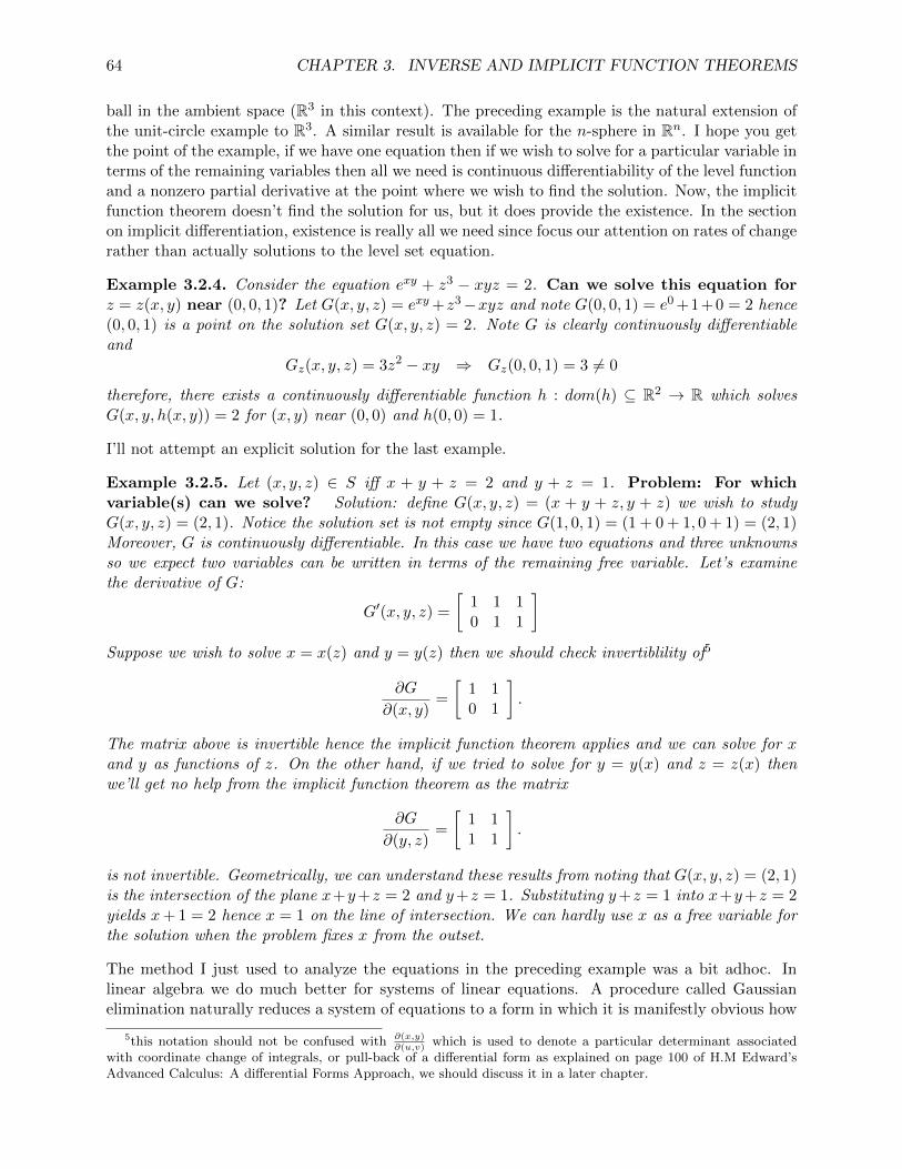
64 CHAPTER 3. INVERSE AND IMPLICIT FUNCTION THEOREMS
ball in the ambient space (R3 in this context). The preceding example is the natural extension ofthe unit-circle example to R3. A similar result is available for the n-sphere in Rn. I hope you getthe point of the example, if we have one equation then if we wish to solve for a particular variable interms of the remaining variables then all we need is continuous differentiability of the level functionand a nonzero partial derivative at the point where we wish to find the solution. Now, the implicitfunction theorem doesn’t find the solution for us, but it does provide the existence. In the sectionon implicit differentiation, existence is really all we need since focus our attention on rates of changerather than actually solutions to the level set equation.
Example 3.2.4. Consider the equation exy + z3 − xyz = 2. Can we solve this equation forz = z(x, y) near (0, 0, 1)? Let G(x, y, z) = exy +z3−xyz and note G(0, 0, 1) = e0 +1+0 = 2 hence(0, 0, 1) is a point on the solution set G(x, y, z) = 2. Note G is clearly continuously differentiableand
Gz(x, y, z) = 3z2 − xy ⇒ Gz(0, 0, 1) = 3 6= 0
therefore, there exists a continuously differentiable function h : dom(h) ⊆ R2 → R which solvesG(x, y, h(x, y)) = 2 for (x, y) near (0, 0) and h(0, 0) = 1.
I’ll not attempt an explicit solution for the last example.
Example 3.2.5. Let (x, y, z) ∈ S iff x + y + z = 2 and y + z = 1. Problem: For whichvariable(s) can we solve? Solution: define G(x, y, z) = (x + y + z, y + z) we wish to studyG(x, y, z) = (2, 1). Notice the solution set is not empty since G(1, 0, 1) = (1 + 0 + 1, 0 + 1) = (2, 1)Moreover, G is continuously differentiable. In this case we have two equations and three unknownsso we expect two variables can be written in terms of the remaining free variable. Let’s examinethe derivative of G:
G′(x, y, z) =
[1 1 10 1 1
]Suppose we wish to solve x = x(z) and y = y(z) then we should check invertiblility of5
∂G
∂(x, y)=
[1 10 1
].
The matrix above is invertible hence the implicit function theorem applies and we can solve for xand y as functions of z. On the other hand, if we tried to solve for y = y(x) and z = z(x) thenwe’ll get no help from the implicit function theorem as the matrix
∂G
∂(y, z)=
[1 11 1
].
is not invertible. Geometrically, we can understand these results from noting that G(x, y, z) = (2, 1)is the intersection of the plane x+y+z = 2 and y+z = 1. Substituting y+z = 1 into x+y+z = 2yields x+ 1 = 2 hence x = 1 on the line of intersection. We can hardly use x as a free variable forthe solution when the problem fixes x from the outset.
The method I just used to analyze the equations in the preceding example was a bit adhoc. Inlinear algebra we do much better for systems of linear equations. A procedure called Gaussianelimination naturally reduces a system of equations to a form in which it is manifestly obvious how
5this notation should not be confused with ∂(x,y)∂(u,v)
which is used to denote a particular determinant associatedwith coordinate change of integrals, or pull-back of a differential form as explained on page 100 of H.M Edward’sAdvanced Calculus: A differential Forms Approach, we should discuss it in a later chapter.

3.2. IMPLICIT FUNCTION THEOREM 65
to eliminate redundant variables in terms of a minimal set of basic free variables. The ”y” of theimplicit function proof discussions plays the role of the so-called pivotal variables whereas the”x” plays the role of the remaining free variables. These variables are generally intermingled inthe list of total variables so to reproduce the pattern assumed for the implicit function theoremwe would need to relabel variables from the outset of a calculation. In the following example, Ishow how reordering the variables allows us to solve for various pairs. In short, put the dependentvariable first and the independent variables second so the Gaussian elimination shows the solutionwith minimal effort. Here’s how:
Example 3.2.6. Consider G(x, y, u, v) = (3x + 2y − u, 2x + y − v) = (−1, 3). We have twoequations with four variables. Let’s investigate which pairs of variables can be taken as independentor dependent variables. The most efficient method to dispatch these questions is probably Gaussianelimination. I leave it to the reader to verify that:
rref
[3 2 −1 0 −12 1 0 −1 3
]=
[1 0 1 −2 70 1 −2 3 −11
]We can immediately read from the result above that x, y can be taken to depend on u, v via theformulas:
x = −u+ 2v + 7, y = 2u− 3v − 11
On the other hand, if we order the variables (u, v, x, y) then Gaussian elimination gives:
rref
[−1 0 3 2 −10 −1 2 1 3
]=
[1 0 −3 −2 10 1 −2 −1 −3
]Therefore, we find u(x, y) and v(x, y) as follows:
u = 3x+ 2y + 1, v = 2x+ y − 3.
To solve for x, u as functions of y, v consider:
rref
[3 −1 2 0 −12 0 1 −1 3
]=
[1 0 1/2 −1/2 3/20 1 −1/2 −3/2 11/2
]From which we can read,
x = −y/2 + v/2 + 3/2, u = y/2 + 3v/2 + 11/2.
I could solve the problem below in the efficient style above, but I will instead follow the method inwhich we discussed in the paragraphs surrounding Equation 3.1. In contrast to the general case,because the problem is linear the solution of Equation 3.1 is also a solution of the actual problem.
Example 3.2.7. Solve the following system of equations near (1,2,3,4,5).
G(x, y, z, a, b) =
x+ y + z + 2a+ 2bx+ 0 + 2z + 2a+ 3b3x+ 2y + z + 3a+ 4b
=
243042
Differentiate to find the Jacobian:
G′(x, y, z, a, b) =
1 1 1 2 21 0 2 2 33 2 1 3 4
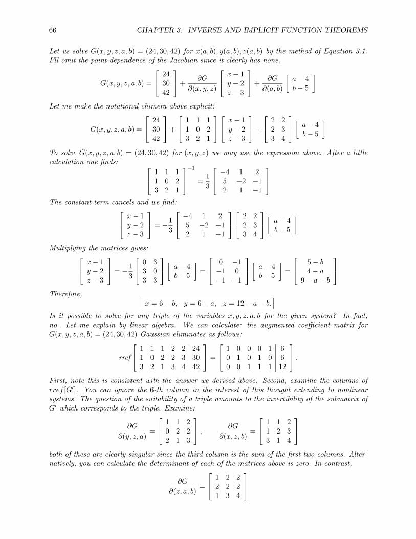
66 CHAPTER 3. INVERSE AND IMPLICIT FUNCTION THEOREMS
Let us solve G(x, y, z, a, b) = (24, 30, 42) for x(a, b), y(a, b), z(a, b) by the method of Equation 3.1.I’ll omit the point-dependence of the Jacobian since it clearly has none.
G(x, y, z, a, b) =
243042
+∂G
∂(x, y, z)
x− 1y − 2z − 3
+∂G
∂(a, b)
[a− 4b− 5
]Let me make the notational chimera above explicit:
G(x, y, z, a, b) =
243042
+
1 1 11 0 23 2 1
x− 1y − 2z − 3
+
2 22 33 4
[ a− 4b− 5
]To solve G(x, y, z, a, b) = (24, 30, 42) for (x, y, z) we may use the expression above. After a littlecalculation one finds: 1 1 1
1 0 23 2 1
−1 =1
3
−4 1 25 −2 −12 1 −1
The constant term cancels and we find: x− 1
y − 2z − 3
= −1
3
−4 1 25 −2 −12 1 −1
2 22 33 4
[ a− 4b− 5
]Multiplying the matrices gives: x− 1
y − 2z − 3
= −1
3
0 33 03 3
[ a− 4b− 5
]=
0 −1−1 0−1 −1
[ a− 4b− 5
]=
5− b4− a
9− a− b
Therefore,
x = 6− b, y = 6− a, z = 12− a− b.Is it possible to solve for any triple of the variables x, y, z, a, b for the given system? In fact,no. Let me explain by linear algebra. We can calculate: the augmented coefficient matrix forG(x, y, z, a, b) = (24, 30, 42) Gaussian eliminates as follows:
rref
1 1 1 2 2 241 0 2 2 3 303 2 1 3 4 42
=
1 0 0 0 1 60 1 0 1 0 60 0 1 1 1 12
.First, note this is consistent with the answer we derived above. Second, examine the columns ofrref [G′]. You can ignore the 6-th column in the interest of this thought extending to nonlinearsystems. The question of the suitability of a triple amounts to the invertibility of the submatrix ofG′ which corresponds to the triple. Examine:
∂G
∂(y, z, a)=
1 1 20 2 22 1 3
, ∂G
∂(x, z, b)=
1 1 21 2 33 1 4
both of these are clearly singular since the third column is the sum of the first two columns. Alter-natively, you can calculate the determinant of each of the matrices above is zero. In contrast,
∂G
∂(z, a, b)=
1 2 22 2 21 3 4
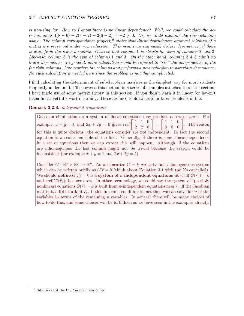
3.2. IMPLICIT FUNCTION THEOREM 67
is non-singular. How to I know there is no linear dependence? Well, we could calculate the de-terminant is 1(8 − 6) − 2(8 − 2) + 2(6 − 2) = −2 6= 0. Or, we could examine the row reductionabove. The column correspondance property6 states that linear dependences amongst columns of amatrix are preserved under row reduction. This means we can easily deduce dependence (if thereis any) from the reduced matrix. Observe that column 4 is clearly the sum of columns 2 and 3.Likewise, column 5 is the sum of columns 1 and 3. On the other hand, columns 3, 4, 5 admit nolinear dependence. In general, more calculation would be required to ”see” the independence of thefar right columns. One reorders the columns and performs a new reduction to ascertain dependence.No such calculation is needed here since the problem is not that complicated.
I find calculating the determinant of sub-Jacobian matrices is the simplest way for most studentsto quickly understand. I’ll showcase this method in a series of examples attached to a later section.I have made use of some matrix theory in this section. If you didn’t learn it in linear (or haven’ttaken linear yet) it’s worth learning. These are nice tools to keep for later problems in life.
Remark 3.2.8. independent constraints
Gaussian elimination on a system of linear equations may produce a row of zeros. For
example, x + y = 0 and 2x + 2y = 0 gives rref
[1 1 02 2 0
]=
[1 1 00 0 0
]. The reason
for this is quite obvious: the equations consider are not indpendent. In fact the secondequation is a scalar multiple of the first. Generally, if there is some linear-dependencein a set of equations then we can expect this will happen. Although, if the equationsare inhomogenous the last column might not be trivial because the system could beinconsistent (for example x+ y = 1 and 2x+ 2y = 5).
Consider G : Rn × Rp → Rn. As we linearize G = k we arrive at a homogeneous systemwhich can be written briefly as G′~r = 0 (think about Equation 3.1 with the k’s cancelled).We should define G(~r) = k is a system of n independent equations at ~ro iff G(~ro) = kand rref[G′(~ro)] has zero row. In other terminology, we could say the system of (possiblynonlinear) equations G(~r) = k is built from n-independent equations near ~ro iff the Jacobianmatrix has full-rank at ~ro. If this full-rank condition is met then we can solve for n of thevariables in terms of the remaining p variables. In general there will be many choices ofhow to do this, and some choices will be forbidden as we have seen in the examples already.
6I like to call it the CCP in my linear notes

68 CHAPTER 3. INVERSE AND IMPLICIT FUNCTION THEOREMS
3.3 implicit differentiation
Enough theory, let’s calculate. In this section I apply previous theoretical constructions to specificproblems. I also introduce standard notation for ”constrained” partial differentiation which isalso sometimes called ”partial differentiation with a side condition”. The typical problem is thefollowing: given equations:
G1(x1, . . . , xm, y1, . . . , yn) = k1
G2(x1, . . . , xm, y1, . . . , yn) = k2...
Gn(x1, . . . , xm, y1, . . . , yn) = kn
calculate partial derivative of dependent variables with respect to independent variables. Contin-uing with the notation of the implicit function discussion we’ll assume that y will be dependenton x. I want to recast some of our arguments via differentials7. Take the total differential of eachequation above,
dG1(x1, . . . , xm, y1, . . . , yn) = 0
dG2(x1, . . . , xm, y1, . . . , yn) = 0
...
dGn(x1, . . . , xm, y1, . . . , yn) = 0
Hence,
∂x1G1dx1 + · · ·+ ∂xmG1dxm + ∂y1G1dy1 + · · ·+ ∂ynG1dyn = 0
∂x1G2dx1 + · · ·+ ∂xmG2dxm + ∂y1G2dy1 + · · ·+ ∂ynG2dyn = 0
...
∂x1Gndx1 + · · ·+ ∂xmGndxm + ∂y1Gndy1 + · · ·+ ∂ynGndyn = 0
Notice, this can be nicely written in column vector notation as:
∂x1Gdx1 + · · ·+ ∂xmGdxm + ∂y1Gdy1 + · · ·+ ∂ynGdyn = 0
Or, in matrix notation:
[∂x1G| · · · |∂xmG]
dx1...
dxm
+ [∂y1G| · · · |∂ynG]
dy1...dyn
= 0
Finally, solve for dy, we assume [∂y1G| · · · |∂ynG]−1 exists, dy1...dyn
= −[∂y1G| · · · |∂ynG]−1[∂x1G| · · · |∂xmG]
dx1...
dxm
Given all of this we can calculate ∂yi
∂xjby simply reading the coeffient dxj in the i-th row. I will
make this idea quite explicit in the examples that follow.
7in contrast, In the previous section we mostly used derivative notation

3.3. IMPLICIT DIFFERENTIATION 69
Example 3.3.1. Let’s return to a common calculus III problem. Suppose F (x, y, z) = k for someconstant k. Find partial derivatives of x, y or z with repsect to the remaining variables.Solution: I’ll use the method of differentials once more:
dF = Fxdx+ Fydy + Fzdz = 0
We can solve for dx, dy or dz provided Fx, Fy or Fz is nonzero respective and these differentialexpressions reveal various partial derivatives of interest:
dx = −FyFxdy − Fz
Fxdz ⇒ ∂x
∂y= −Fy
Fx&
∂x
∂z= −Fz
Fx
dy = −FxFydx− Fz
Fydz ⇒ ∂y
∂x= −Fx
Fy&
∂y
∂z= −Fz
Fy
dz = −FxFzdx− Fy
Fzdy ⇒ ∂z
∂x= −Fx
Fz&
∂z
∂y= −Fy
Fz
In each case above, the implicit function theorem allows us to solve for one variable in terms of theremaining two. If the partial derivative of F in the denominator are zero then the implicit functiontheorem does not apply and other thoughts are required. Often calculus text give the following as ahomework problem:
∂x
∂y
∂y
∂z
∂z
∂x= −Fy
Fx
FzFy
FxFz
= −1.
In the equation above we have x appear as a dependent variable on y, z and also as an independentvariable for the dependent variable z. These mixed expressions are actually of interest to engineeringand physics. The less mbiguous notation below helps better handle such expressions:(
∂x
∂y
)z
(∂y
∂z
)x
(∂z
∂x
)y
= −1.
In each part of the expression we have clearly denoted which variables are taken to depend on theothers and in turn what sort of partial derivative we mean to indicate. Partial derivatives are nottaken alone, they must be done in concert with an understanding of the totality of the indpendentvariables for the problem. We hold all the remaining indpendent variables fixed as we take a partialderivative.
The explicit independent variable notation is more important for problems where we can choosemore than one set of indpendent variables for a given dependent variables. In the example thatfollows we study w = w(x, y) but we could just as well consider w = w(x, z). Generally it will notbe the case that
(∂w∂x
)y
is the same as(∂w∂x
)z. In calculation of
(∂w∂x
)y
we hold y constant as we
vary x whereas in(∂w∂x
)z
we hold z constant as we vary x. There is no reason these ought to be thesame8.
Example 3.3.2. Suppose x+y+z+w = 3 and x2−2xyz+w3 = 5. Calculate partial derivativesof z and w with respect to the independent variables x, y. Solution: we begin by calculationof the differentials of both equations:
dx+ dy + dz + dw = 0(2x− 2yz)dx− 2xzdy − 2xydz + 3w2dw = 0
8a good exercise would be to do the example over but instead aim to calculate partial derivatives for y, w withrespect to independent variables x, z
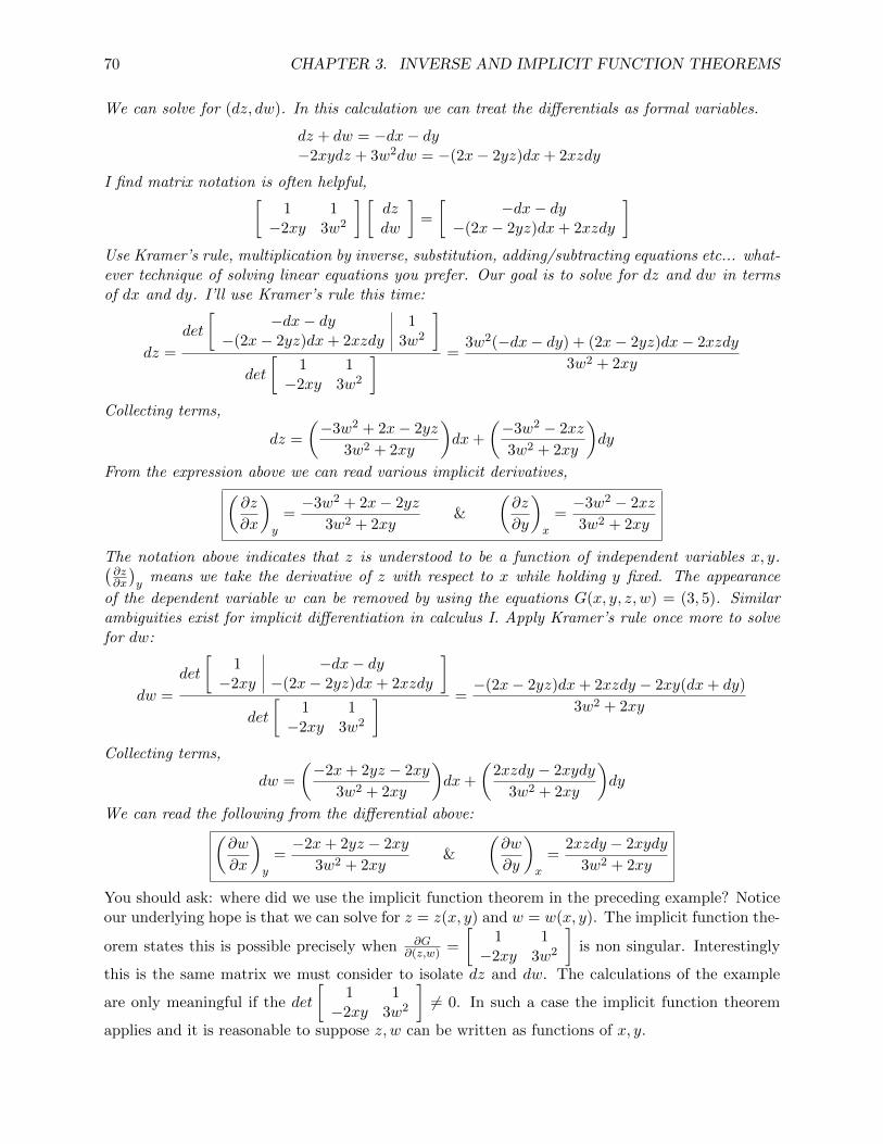
70 CHAPTER 3. INVERSE AND IMPLICIT FUNCTION THEOREMS
We can solve for (dz, dw). In this calculation we can treat the differentials as formal variables.
dz + dw = −dx− dy−2xydz + 3w2dw = −(2x− 2yz)dx+ 2xzdy
I find matrix notation is often helpful,[1 1−2xy 3w2
] [dzdw
]=
[−dx− dy
−(2x− 2yz)dx+ 2xzdy
]Use Kramer’s rule, multiplication by inverse, substitution, adding/subtracting equations etc... what-ever technique of solving linear equations you prefer. Our goal is to solve for dz and dw in termsof dx and dy. I’ll use Kramer’s rule this time:
dz =
det
[−dx− dy 1
−(2x− 2yz)dx+ 2xzdy 3w2
]det
[1 1−2xy 3w2
] =3w2(−dx− dy) + (2x− 2yz)dx− 2xzdy
3w2 + 2xy
Collecting terms,
dz =
(−3w2 + 2x− 2yz
3w2 + 2xy
)dx+
(−3w2 − 2xz
3w2 + 2xy
)dy
From the expression above we can read various implicit derivatives,(∂z
∂x
)y
=−3w2 + 2x− 2yz
3w2 + 2xy&
(∂z
∂y
)x
=−3w2 − 2xz
3w2 + 2xy
The notation above indicates that z is understood to be a function of independent variables x, y.(∂z∂x
)y
means we take the derivative of z with respect to x while holding y fixed. The appearance
of the dependent variable w can be removed by using the equations G(x, y, z, w) = (3, 5). Similarambiguities exist for implicit differentiation in calculus I. Apply Kramer’s rule once more to solvefor dw:
dw =
det
[1 −dx− dy−2xy −(2x− 2yz)dx+ 2xzdy
]det
[1 1−2xy 3w2
] =−(2x− 2yz)dx+ 2xzdy − 2xy(dx+ dy)
3w2 + 2xy
Collecting terms,
dw =
(−2x+ 2yz − 2xy
3w2 + 2xy
)dx+
(2xzdy − 2xydy
3w2 + 2xy
)dy
We can read the following from the differential above:(∂w
∂x
)y
=−2x+ 2yz − 2xy
3w2 + 2xy&
(∂w
∂y
)x
=2xzdy − 2xydy
3w2 + 2xy
You should ask: where did we use the implicit function theorem in the preceding example? Noticeour underlying hope is that we can solve for z = z(x, y) and w = w(x, y). The implicit function the-
orem states this is possible precisely when ∂G∂(z,w) =
[1 1−2xy 3w2
]is non singular. Interestingly
this is the same matrix we must consider to isolate dz and dw. The calculations of the example
are only meaningful if the det
[1 1−2xy 3w2
]6= 0. In such a case the implicit function theorem
applies and it is reasonable to suppose z, w can be written as functions of x, y.

3.3. IMPLICIT DIFFERENTIATION 71
3.3.1 computational techniques for partial differentiation with side conditions
In this section I show you how I teach this to calculus III. In other words, we set-aside the explicitmention of the implicit function theorem and work out some typical calculations. If one desiresrigor then the answer is found from the implicit function theorems careful application, that is howto justify what follows. These notes are taken from my calculus III notes, but I thought it wiseto include them here since most calculus texts do not bother to show these calculations (whichis sad since they actually matter to the application of multivariate analysis to many real worldapplications) To begin, we define9 the total differential.
Definition 3.3.3.
If f = f(x1, x2, . . . , xn) then df = ∂f∂x1
dx1 + ∂f∂x2
dx2 + · · ·+ ∂f∂xn
dxn.
Example 3.3.4. Suppose E = pv+ t2 then dE = vdp+ pdv+ 2tdt. In this example the dependentvariable is E whereas the independent variables are p, v and t.
Example 3.3.5. Problem: what are ∂F/∂x and ∂F/∂y if we know that F = F (x, y) anddF = (x2 + y)dx− cos(xy)dy.Solution: if F = F (x, y) then the total differential has the form dF = Fxdx + Fydy. We simplycompare the general form to the given dF = (x2 + y)dx− cos(xy)dy to obtain:
∂F
∂x= x2 + y,
∂F
∂y= − cos(xy).
Example 3.3.6. Suppose w = xyz then dw = yzdx + xzdy + xydz. On the other hand, we cansolve for z = z(x, y, w)
z =w
xy⇒ dz = − w
x2ydx− w
xy2dy +
1
xydw. ?
If we solve dw = yzdx+ xzdy + xydz directly for dz we obtain:
dz = − zxdx− z
ydy +
1
xydw ? ?.
Are ? and ?? consistent? Well, yes. Note wx2y
= xyzx2y
= zx and w
xy2= xyz
xy2= z
y .
Which variables are independent/dependent in the example above? It depends. In this initialportion of the example we treated x, y, z as independent whereas w was dependent. But, in thelast half we treated x, y, w as independent and z was the dependent variable. Consider this, if Iask you what the value of ∂z
∂x is in the example above then this question is ambiguous!
∂z
∂x= 0︸ ︷︷ ︸
z indpendent of x
verses∂z
∂x=−zx︸ ︷︷ ︸
z depends on x
Obviously this sort of ambiguity is rather unpleasant. A natural solution to this trouble is simplyto write a bit more when variables are used in multiple contexts. In particular,
∂z
∂x
∣∣∣∣y,z
= 0︸ ︷︷ ︸means x,y,z independent
is different than∂z
∂x
∣∣∣∣y,w
=−zx︸ ︷︷ ︸
means x,y,w independent
.
9I invite the reader to verify the notation ”defined” in this section is in fact totally sympatico with our previousdefinitions
72 CHAPTER 3. INVERSE AND IMPLICIT FUNCTION THEOREMS
The key concept is that all the other independent variables are held fixed as an indpendent variableis partial differentiated. Holding y, z fixed as x varies means z does not change hence ∂z
∂x
∣∣y,z
= 0.On the other hand, if we hold y, w fixed as x varies then the change in z need not be trivial;∂z∂x
∣∣y,w
= −zx . Let me expand on how this notation interfaces with the total differential.
Definition 3.3.7.
If w, x, y, z are variables then
dw =∂w
∂x
∣∣∣∣y,z
dx+∂w
∂y
∣∣∣∣x,z
dy +∂w
∂z
∣∣∣∣x,y
dz.
Alternatively,
dx =∂x
∂w
∣∣∣∣y,z
dw +∂x
∂y
∣∣∣∣w,z
dy +∂x
∂z
∣∣∣∣w,y
dz.
The larger idea here is that we can identify partial derivatives from the coefficients in equations ofdifferentials. I’d say a differential equation but you might get the wrong idea... Incidentally, thereis a whole theory of solving differential equations by clever use of differentials, I have books if youare interested.
Example 3.3.8. Suppose w = x+ y + z and x+ y = wz then calculate ∂w∂x
∣∣y
and ∂w∂x
∣∣z. Notice we
must choose dependent and independent variables to make sense of partial derivatives in question.
1. suppose w, z both depend on x, y. Calculate,
∂w
∂x
∣∣∣∣y
=∂
∂x
∣∣∣∣y
(x+ y + z) =∂x
∂x
∣∣∣∣y
+∂y
∂x
∣∣∣∣y
+∂z
∂x
∣∣∣∣y
= 1 + 0 +∂z
∂x
∣∣∣∣y
?
To calculate further we need to eliminate w by substituting w = x + y + z into x + y = wz;thus x+ y = (x+ y + z)z hence dx+ dy = (dx+ dy + dz)z + (x+ y + z)dz
(2z + x+ y)dz = (1− z)dx+ (1− z)dy ? ?
Therefore,
dz =1− z
2z + x+ ydx+
1− z2z + x+ y
dy =∂z
∂x
∣∣∣∣y
dx+∂z
∂y
∣∣∣∣x
dy ⇒ ∂z
∂x
∣∣∣∣y
=1− z
2z + x+ y.
Returning to ? we derive
∂w
∂x
∣∣∣∣y
= 1 +1− z
2z + x+ y.
2. suppose w, y both depend on x, z. Calculate,
∂w
∂x
∣∣∣∣z
=∂
∂x
∣∣∣∣z
(x+ y + z) =∂x
∂x
∣∣∣∣z
+∂y
∂x
∣∣∣∣z
+∂z
∂x
∣∣∣∣z
= 1 +∂y
∂x
∣∣∣∣z
+ 0
To complete this calculation we need to eliminate w as before, using ??,
(1− z)dy = (1− z)dx− (2z + x+ y)dz ⇒ ∂y
∂x
∣∣∣∣z
= 1.
Therefore,
∂w
∂x
∣∣∣∣z
= 2.

3.4. THE CONSTANT RANK THEOREM 73
I hope you can begin to see how the game is played. Basically the example above generalizes theidea of implicit differentiation to several equations of many variables. This is actually a prettyimportant type of calculation for engineering. The study of thermodynamics is full of variableswhich are intermittently used as either dependent or independent variables. The so-called equationof state can be given in terms of about a dozen distinct sets of state variables.
Example 3.3.9. The ideal gas law states that for a fixed number of particles n the pressure P ,volume V and temperature T are related by PV = nRT where R is a constant. Calculate,
∂P
∂V
∣∣∣∣T
=∂
∂V
[nRT
V
]∣∣∣∣T
= −nRTV 2
,
∂V
∂T
∣∣∣∣P
=∂
∂T
[nRT
P
]∣∣∣∣T
=nR
P,
∂T
∂P
∣∣∣∣V
=∂
∂P
[PV
nR
]∣∣∣∣T
=V
nR.
You might expect that ∂P∂V
∣∣T∂V∂T
∣∣P∂T∂P
∣∣V
= 1. Is it true?
∂P
∂V
∣∣∣∣T
∂V
∂T
∣∣∣∣P
∂T
∂P
∣∣∣∣V
= −nRTV 2· nRP· VnR
=−nRTPV
= −1.
This is an example where naive cancellation of partials fails.
Example 3.3.10. Suppose F (x, y) = 0 then dF = Fxdx+Fydy = 0 and it follows that dx = −FyFxdy
or dy = −FxFydx. Hence, ∂x
∂y = −FyFx
and ∂y∂x = −Fx
Fy. Therefore,
∂x
∂y
∂y
∂x=FyFx· FxFy
= 1
for (x, y) such that Fx 6= 0 and Fy 6= 0. The condition Fx 6= 0 suggests we can solve for y = y(x)whereas the condition Fy 6= 0 suggests we can solve for x = x(y).
3.4 the constant rank theorem
The implicit function theorem required we work with independent constraints. However, one doesnot always have that luxury. There is a theorem which deals with the slightly more general case.The base idea is that if the Jacobian has rank k then it locally injects a k-dimensional image intothe codomain. If we are using a map as a parametrization then the rank k condition suggests themapping does parametrize a k-fold, at least locally. On the other hand, if we are using the mapto define a space as a level set then F : Rn → Rp has F−1(C) as a (n − k)-fold. Previously, wewould have insisted k = p. I’ve run out of time for 2013 notes10 so sadly I have no reference forthis claim. In any event, theorems aside, I think the red comments are worth some discussion.
Remark 3.4.1.
I have put remarks about the rank of the derivative in red for the examples below.
10in 2017 it seems the situation has not changed, perhaps we’ll find it together this semester

74 CHAPTER 3. INVERSE AND IMPLICIT FUNCTION THEOREMS
Example 3.4.2. Let f(t) = (t, t2, t3) then f ′(t) = (1, 2t, 3t2). In this case we have
f ′(t) = [dft] =
12t3t2
The Jacobian here is a single column vector. It has rank 1 provided the vector is nonzero. Wesee that f ′(t) 6= (0, 0, 0) for all t ∈ R. This corresponds to the fact that this space curve has awell-defined tangent line for each point on the path.
Example 3.4.3. Let f(~x, ~y) = ~x · ~y be a mapping from R3 × R3 → R. I’ll denote the coordinatesin the domain by (x1, x2, x3, y1, y2, y3) thus f(~x, ~y) = x1y1 + x2y2 + x3y3. Calculate,
[df(~x,~y)] = ∇f(~x, ~y)T = [y1, y2, y3, x1, x2, x3]
The Jacobian here is a single row vector. It has rank 6 provided all entries of the input vectors arenonzero.
Example 3.4.4. Let f(~x, ~y) = ~x · ~y be a mapping from Rn × Rn → R. I’ll denote the coordinatesin the domain by (x1, . . . , xn, y1, . . . , yn) thus f(~x, ~y) =
∑ni=1 xiyi. Calculate,
∂xj
[ n∑i=1
xiyi
]=
n∑i=1
∂xixjyi =
n∑i=1
δijyi = yj
Likewise,
∂yj
[ n∑i=1
xiyi
]=
n∑i=1
xi∂yiyj
=
n∑i=1
xiδij = xj
Therefore, noting that ∇f = (∂x1f, . . . , ∂xnf, ∂y1f, . . . , ∂ynf),
[df(~x,~y)]T = (∇f)(~x, ~y) = ~y × ~x = (y1, . . . , yn, x1, . . . , xn)
The Jacobian here is a single row vector. It has rank 2n provided all entries of the input vectorsare nonzero.
Example 3.4.5. Suppose F (x, y, z) = (xyz, y, z) we calculate,
∂F∂x = (yz, 0, 0) ∂F
∂y = (xz, 1, 0) ∂F∂z = (xy, 0, 1)
Remember these are actually column vectors in my sneaky notation; (v1, . . . , vn) = [v1, . . . , vn]T .This means the derivative or Jacobian matrix of F at (x, y, z) is
F ′(x, y, z) = [dF(x,y,z)] =
yz xz xy0 1 00 0 1
Note, rank(F ′(x, y, z)) = 3 for all (x, y, z) ∈ R3 such that y, z 6= 0. There are a variety of ways tosee that claim, one way is to observe det[F ′(x, y, z)] = yz and this determinant is nonzero so longas neither y nor z is zero. In linear algebra we learn that a square matrix is invertible iff it hasnonzero determinant iff it has linearly indpendent column vectors.

3.4. THE CONSTANT RANK THEOREM 75
Example 3.4.6. Suppose F (x, y, z) = (x2 + z2, yz) we calculate,
∂F∂x = (2x, 0) ∂F
∂y = (0, z) ∂F∂z = (2z, y)
The derivative is a 2× 3 matrix in this example,
F ′(x, y, z) = [dF(x,y,z)] =
[2x 0 2z0 z y
]The maximum rank for F ′ is 2 at a particular point (x, y, z) because there are at most two linearlyindependent vectors in R2. You can consider the three square submatrices to analyze the rank fora given point. If any one of these is nonzero then the rank (dimension of the column space) is two.
M1 =
[2x 00 z
]M2 =
[2x 2z0 y
]M3 =
[0 2zz y
]We’ll need either det(M1) = 2xz 6= 0 or det(M2) = 2xy 6= 0 or det(M3) = −2z2 6= 0. I believethe only point where all three of these fail to be true simulataneously is when x = y = z = 0. Thismapping has maximal rank at all points except the origin.
Example 3.4.7. Suppose F (x, y) = (x2 + y2, xy, x+ y) we calculate,
∂F∂x = (2x, y, 1) ∂F
∂y = (2y, x, 1)
The derivative is a 3× 2 matrix in this example,
F ′(x, y) = [dF(x,y)] =
2x 2yy x1 1
The maximum rank is again 2, this time because we only have two columns. The rank will be twoif the columns are not linearly dependent. We can analyze the question of rank a number of waysbut I find determinants of submatrices a comforting tool in these sort of questions. If the columnsare linearly dependent then all three sub-square-matrices of F ′ will be zero. Conversely, if even oneof them is nonvanishing then it follows the columns must be linearly independent. The submatricesfor this problem are:
M1 =
[2x 2yy x
]M2 =
[2x 2y1 1
]M3 =
[y x1 1
]You can see det(M1) = 2(x2 − y2), det(M2) = 2(x− y) and det(M3) = y − x. Apparently we haverank(F ′(x, y, z)) = 2 for all (x, y) ∈ R2 with y 6= x. In retrospect this is not surprising.
Example 3.4.8. Let F (x, y) = (x, y,√R2 − x2 − y2) for a constant R. We calculate,
∇√R2 − x2 − y2 =
(−x√
R2−x2−y2, −y√
R2−x2−y2
)Also, ∇x = (1, 0) and ∇y = (0, 1) thus
F ′(x, y) =
1 00 1−x√
R2−x2−y2−y√
R2−x2−y2

76 CHAPTER 3. INVERSE AND IMPLICIT FUNCTION THEOREMS
This matrix clearly has rank 2 where is is well-defined. Note that we need R2 − x2 − y2 > 0 for thederivative to exist. Moreover, we could define G(y, z) = (
√R2 − y2 − z2, y, z) and calculate,
G′(y, z) =
1 0−y√
R2−y2−z2−z√
R2−y2−z2
0 1
.Observe that G′(y, z) exists when R2 − y2 − z2 > 0. Geometrically, F parametrizes the sphereabove the equator at z = 0 whereas G parametrizes the right-half of the sphere with x > 0. Theseparametrizations overlap in the first octant where both x and z are positive. In particular, dom(F ′)∩dom(G′) = {(x, y) ∈ R2 | x, y > 0 and x2 + y2 < R2}
Example 3.4.9. Let F (x, y, z) = (x, y, z,√R2 − x2 − y2 − z2) for a constant R. We calculate,
∇√R2 − x2 − y2 − z2 =
(−x√
R2−x2−y2−z2, −y√
R2−x2−y2−z2, −z√
R2−x2−y2−z2
)Also, ∇x = (1, 0, 0), ∇y = (0, 1, 0) and ∇z = (0, 0, 1) thus
F ′(x, y, z) =
1 0 00 1 00 0 1−x√
R2−x2−y2−z2−y√
R2−x2−y2−z2−z√
R2−x2−y2−z2
This matrix clearly has rank 3 where is is well-defined. Note that we need R2−x2−y2−z2 > 0 for thederivative to exist. This mapping gives us a parametrization of the 3-sphere x2 + y2 + z2 +w2 = R2
for w > 0. (drawing this is a little trickier)
Example 3.4.10. Let f(x, y, z) = (x+ y, y + z, x+ z, xyz). You can calculate,
[df(x,y,z)] =
1 1 00 1 11 0 1yz xz xy
This matrix clearly has rank 3 and is well-defined for all of R3.
Example 3.4.11. Let f(x, y, z) = xyz. You can calculate,
[df(x,y,z)] =[yz xz xy
]This matrix fails to have rank 3 if x, y or z are zero. In other words, f ′(x, y, z) has rank 3 inR3 provided we are at a point which is not on some coordinate plane. (the coordinate planes arex = 0, y = 0 and z = 0 for the yz, zx and xy coordinate planes respective)
Example 3.4.12. Let f(x, y, z) = (xyz, 1− x− y). You can calculate,
[df(x,y,z)] =
[yz xz xy−1 −1 0
]This matrix has rank 3 if either xy 6= 0 or (x− y)z 6= 0. In contrast to the preceding example, thederivative does have rank 3 on certain points of the coordinate planes. For example, f ′(1, 1, 0) andf ′(0, 1, 1) both give rank(f ′) = 3.
3.4. THE CONSTANT RANK THEOREM 77
Example 3.4.13. Let X(u, v) = (x, y, z) where x, y, z denote functions of u, v and I prefer to omitthe explicit depedendence to reduce clutter in the equations to follow.
∂X
∂u= Xu = (xu, yu, zu) and
∂X
∂v= Xv = (xv, yv, zv)
Then the Jacobian is the 3× 2 matrix
[dX(u,v)
]=
xu xvyu yvzu zv
The matrix
[dX(u,v)
]has rank 2 if at least one of the determinants below is nonzero,
det
[xu xvyu yv
]det
[xu xvzu zv
]det
[yu yvzu zv
]

78 CHAPTER 3. INVERSE AND IMPLICIT FUNCTION THEOREMS

Chapter 4
two views of manifolds in Rn
In this chapter we describe spaces inside Rn which are k-dimensional 1. Technically, to make thisprecise we would need to study manifolds with boundary. Careful discussion of manifolds withboundary in euclidean space can be found in Munkres Analysis on Manifolds. In the interest offocusing on examples, I’ll be a bit fuzzy about the defintion of a k-dimensional subspace S ofeuclidean space. This much we can say: there are two ways to envision the geometry of S:
(1.) Parametrically: provide a patch R such that R : U ⊆ Rk → S ⊆ Rn. Here U is called theparameter space and R−1 is called a coordinate chart. The cannonical example:
R(x1, . . . xk) = (x1, . . . xk, 0, . . . , 0).
(2.) Implicitly: provide a level function G : Rk × Rp → Rp such that S = G−1{c} = S. Thisviewpoint casts S as points in x ∈ Rk × Rp for which G(x) = k. The cannonical example:
G(x1, . . . , xk+p) = (xk+1, . . . , xk+p) = (0, . . . , 0).
The cannonical examples of (1.) and (2.) are both the x1 . . . xk-coordinate plane embedded in Rn.Just to take it down a notch. If n = 3 then we could look at the xy-plane in either view as follows:
(1.) R(x, y) = (x, y, 0) (2.) G(x, y, z) = z = 0.
Which viewpoint should we adopt? What is the dimension of a given space S? How should wefind tangent space to S? How should we find the normal space to S? These are the questions weset-out to answer in this chapter.
Orthogonal complements help us to understand how all of this fits together. This is possible since wedeal with embedded manifolds for which the euclidean dot-product of Rn is available to sort out thegeometry. Finally, we use this geometry and a few simple lemmas to justify the method of Lagrangemultipliers. Lagrange’s technique paired with the theory of multivariate Taylor polynomials formthe basis for analyzing extrema for multivariate functions. In this chapter we deal with the questionof extrema on the edges of a set. The second half of the story is found in the next chapter wherewe deal with the interior points via the theory of quadratic forms applied to the second-orderapproximation to a function of several variables.
1I’ll try to stick with this notation for this chapter, n ≥ k and n = p+ k
79

80 CHAPTER 4. TWO VIEWS OF MANIFOLDS IN RN
4.1 definition of level set
A level set is the solution set of some equation or system of equations. We confine our interest tolevel sets of Rn. For example, the set of all (x, y) that satisfy
G(x, y) = c
is called a level curve in R2. Often we can use k to label the curve. You should also recall levelsurfaces in R3 are defined by an equation of the form
G(x, y, z) = c.
The set of all (x1, x2, x3, x4) ∈ R4 which solve G(x1, x2, x3, x4) = c is a level volume in R4. Wecan obtain lower dimensional objects by simultaneously imposing several equations at once. Forexample, suppose G1(x, y, z) = z = 1 and G2(x, y, z) = x2 +y2 +z2 = 5, points (x, y, z) which solveboth of these equations are on the intersection of the plane z = 1 and the sphere x2 + y2 + z2 = 5.Let G = (G1, G2), note that G(x, y, z) = (1, 5) describes a circle in R3. More generally:
Definition 4.1.1.
Suppose G : dom(G) ⊆ Rk × Rp → Rp. Let c be a vector of constants in Rp and supposeS = {x ∈ Rk × Rp | G(x) = c} is non-empty and G is continuously differentiable on anopen set containing S. We say S is an k-dimensional level set iff G′(x) has p linearlyindependent rows at each x ∈ S.
The condition of linear independence of the rows is give to eliminate possible redundancy in thesystem of equations. In the case that p = 1 the criteria reduces to G′(x) 6= 0 over the level setof dimension n − 1. Intuitively we think of each equation in G(x) = c as removing one of thedimensions of the ambient space Rn = Rk ×Rp. It is worthwhile to cite a useful result from linearalgebra at this point:
Proposition 4.1.2.
Let A ∈ Rm×n. The number of linearly independent columns in A is the same as thenumber of linearly independent rows in A. This invariant of A is called the rank of A.
Given the wisdom of linear algebra we see that we should require a k-dimensional level set S =G−1(c) to have a level function G : Rn → Rp whose derivative is of rank n − k = p over all of S.We can either analyze linear independence of columns or rows.
Example 4.1.3. Consider G(x, y, z) = x2 + y2 − z2 and suppose S = G−1{0}. Calculate,
G′(x, y, z) = [2x, 2y,−2z]
Notice that (0, 0, 0) ∈ S and G′(0, 0, 0) = [0, 0, 0] hence G′ is not rank one at the origin. At allother points in S we have G′(x, y, z) 6= 0 which means this is almost a 3 − 1 = 2-dimensionallevel set. However, almost is not good enough in math. Under our definition the cone S is not a2-dimensional level set since it fails to meet the full-rank criteria at the point of the cone.
A p-dimensional level set is an example of a p-dimensional manifold. The example above with theorigin included is a manifold paired with a singular point, such spaces are known as orbifolds.The study of orbifolds has attracted considerable effort in recent years as the singularities of suchorbifolds can be used to do physics in string theory. I digress. Let us examine another level set:
Example 4.1.4. Let G(x, y, z) = (x, y) and define S = G−1(a, b) for some fixed pair of constantsa, b ∈ R. We calculate that G′(x, y, z) = I2 ∈ R2×2. We clearly have rank two at all points in Shence S is a 3− 2 = 1-dimensional level set. Perhaps you realize S is the vertical line which passesthrough (a, b, 0) in the xy-plane.

4.2. TANGENTS AND NORMALS TO A LEVEL SET 81
4.2 tangents and normals to a level set
There are many ways to define a tangent space for some subset of Rn. One natural definition isthat the tangent space to p ∈ S is simply the set of all tangent vectors to curves on S which passthrough the point p. In this section we study the geometry of curves on a level-set. We’ll see howthe tangent space is naturally a vector space in the particular context of level-sets in Rn.
Throughout this section we assume that S is a k-dimensional level set defined by G : Rk×Rp → Rpwhere G−1(c) = S. This means that we can apply the implicit function theorem to S and forany given point p = (px, py) ∈ S where px ∈ Rk and py ∈ Rp. There exists a local continuouslydifferentiable solution h : U ⊆ Rk → Rp such that h(px) = py and for all x ∈ U we have G(x, h(x)) =c. We can view G(x, y) = c for x near p as the graph of y = h(x) for x ∈ U . With the set-up abovein mind, suppose that γ : R→ U ⊆ S. If we write γ = (γx, γy) then it follows γ = (γx, h ◦ γx) overthe subset U × h(U) of S. More explicitly, for all t ∈ R such that γ(t) ∈ U × h(U) we have
γ(t) = (γx(t), h(γx(t))).
Therefore, if γ(0) = p then γ(0) = (px, h(px)). Differentiate, use the chain-rule in the second factorto obtain:
γ′(t) = (γ′x(t), h′(γx(t))γ′x(t)).
We find that the tangent vector to p ∈ S of γ has a rather special form which was forced on us bythe implicit function theorem:
γ′(0) = (γ′x(0), h′(px)γ′x(0)).
Or to cut through the notation a bit, if γ′(0) = v = (vx, vy) then v = (vx, h′(px)vx). The second
component of the vector is not free of the first, it essentially redundant. This makes us suspectthat the tangent space to S at p is k-dimensional.
Theorem 4.2.1.
Let G : Rk × Rp → Rp be a level-mappping which defines a k-dimensional level set Sby G−1(c) = S. Suppose γ1, γ2 : R → S are differentiable curves with γ′1(0) = v1 andγ′2(0) = v2 then there exists a differentiable curve γ : R→ S such that γ′(0) = v1 + v2 andγ(0) = p. Moreover, there exists a differentiable curve β : R→ S such that β′(0) = cv1 andβ(0) = p.
Proof: It is convenient to define a map which gives a local parametrization of S at p. Sincewe have a description of S locally as a graph y = h(x) (near p) it is simple to construct theparameterization. Define Φ : U ⊆ Rk → S by Φ(x) = (x, h(x)). Clearly Φ(U) = U × h(U) andthere is an inverse mapping Φ−1(x, y) = x is well-defined since y = h(x) for each (x, y) ∈ U ×h(U).Let w ∈ Rk and observe that
ψ(t) = Φ(Φ−1(p) + tw) = Φ(px + tw) = (px + tw, h(px + tw))
is a curve from R to U ⊆ S such that ψ(0) = (px, h(px)) = (px, py) = p and using the chain rule onthe final form of ψ(t):
ψ′(0) = (w, h′(px)w).
The construction above shows that any vector of the form (vx, h′(px)vx) is the tangent vector of a
particular differentiable curve in the level set (differentiability of ψ follows from the differentiabilityof h and the other maps which we used to construct ψ). In particular we can apply this to thecase w = v1x + v2x and we find γ(t) = Φ(Φ−1(p) + t(v1x + v2x)) has γ′(0) = v1 + v2 and γ(0) = p.
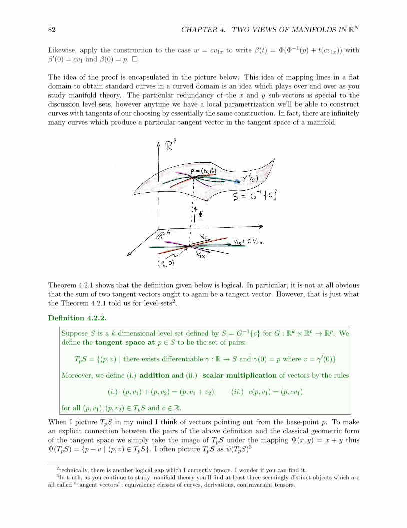
82 CHAPTER 4. TWO VIEWS OF MANIFOLDS IN RN
Likewise, apply the construction to the case w = cv1x to write β(t) = Φ(Φ−1(p) + t(cv1x)) withβ′(0) = cv1 and β(0) = p. �
The idea of the proof is encapsulated in the picture below. This idea of mapping lines in a flatdomain to obtain standard curves in a curved domain is an idea which plays over and over as youstudy manifold theory. The particular redundancy of the x and y sub-vectors is special to thediscussion level-sets, however anytime we have a local parametrization we’ll be able to constructcurves with tangents of our choosing by essentially the same construction. In fact, there are infinitelymany curves which produce a particular tangent vector in the tangent space of a manifold.
Theorem 4.2.1 shows that the definition given below is logical. In particular, it is not at all obviousthat the sum of two tangent vectors ought to again be a tangent vector. However, that is just whatthe Theorem 4.2.1 told us for level-sets2.
Definition 4.2.2.
Suppose S is a k-dimensional level-set defined by S = G−1{c} for G : Rk × Rp → Rp. Wedefine the tangent space at p ∈ S to be the set of pairs:
TpS = {(p, v) | there exists differentiable γ : R→ S and γ(0) = p where v = γ′(0)}
Moreover, we define (i.) addition and (ii.) scalar multiplication of vectors by the rules
(i.) (p, v1) + (p, v2) = (p, v1 + v2) (ii.) c(p, v1) = (p, cv1)
for all (p, v1), (p, v2) ∈ TpS and c ∈ R.
When I picture TpS in my mind I think of vectors pointing out from the base-point p. To makean explicit connection between the pairs of the above definition and the classical geometric formof the tangent space we simply take the image of TpS under the mapping Ψ(x, y) = x + y thusΨ(TpS) = {p+ v | (p, v) ∈ TpS}. I often picture TpS as ψ(TpS)3
2technically, there is another logical gap which I currently ignore. I wonder if you can find it.3In truth, as you continue to study manifold theory you’ll find at least three seemingly distinct objects which are
all called ”tangent vectors”; equivalence classes of curves, derivations, contravariant tensors.

4.2. TANGENTS AND NORMALS TO A LEVEL SET 83
We could set out to calculate tangent spaces in view of the definition above, but we are actuallyinterested in more than just the tangent space for a level-set. In particular. we want a concretedescription of all the vectors which are not in the tangent space.
Definition 4.2.3.
Suppose S is a k-dimensional level-set defined by S = G−1{c} for G : Rk × Rp → Rp andTpS is the tangent space at p. Note that TpS ≤ Vp where Vp = {p} × Rk × Rp is given thenatural vector space structure which we already exhibited on the subspace TpS. We definethe inner product on Vp as follows: for all (p, v), (p, w) ∈ Vp,
(p, v) · (p, w) = v · w.
The length of a vector (p, v) is naturally defined by ||(p, v)|| = ||v||. Moreover, we say twovectors (p, v), (p, w) ∈ Vp are orthogonal iff v · w = 0. Given a set of vectors R ⊆ Vp wedefine the orthogonal complement by
R⊥ = {(p, v) ∈ Vp | (p, v) · (p, r) for all (p, r) ∈ R}.
Suppose W1,W2 ⊆ Vp then we say W1 is orthogonal to W2 iff w1 ·w2 = 0 for all w1 ∈W1
and w2 ∈W2. We denote orthogonality by writing W1 ⊥W2. If every v ∈ Vp can be writtenas v = w1 + w2 for a pair of w1 ∈W1 and w2 ∈W2 where W1 ⊥W2 then we say that Vp isthe direct sum of W1 and W2 which is denoted by Vp = W1 ⊕W2.
There is much more to say about orthogonality, however, our focus is not in that vein. We justneed the langauge to properly define the normal space. The calculation below is probably the mostimportant calculation to understand for a level-set. Suppose we have a curve γ : R → S whereS = G−1(c) is a k-dimensional level-set in Rk × Rp. Observe that for all t ∈ R,
G(γ(t)) = c ⇒ G′(γ(t))γ′(t) = 0.
In particular, suppose for t = 0 we have γ(0) = p and v = γ′(0) which makes (p, v) ∈ TpS with
G′(p)v = 0.
Recall G : Rk × Rp → Rp has an p× n derivative matrix where the j-th row is the gradient vectorof the j-th component function. The equation G′(p)v = 0 gives us p-independent equations aswe examine it componentwise. In particular, it reveals that (p, v) is orthogonal to ∇Gj(p) forj = 1, 2, . . . , p. We have derived the following theorem:
Theorem 4.2.4.
Let G : Rk × Rp → Rp be a level-mappping which defines a k-dimensional level set S byG−1(c) = S. The gradient vectors ∇Gj(p) are perpendicular to the tangent space at p; foreach j ∈ Np
(p,∇(Gj(p))T ) ∈ (TpS)⊥.
It’s time to do some counting. Observe that the mapping φ : Rk → TpS defined by φ(v) = (p, v)is an isomorphism of vector spaces hence dim(TpS) = k. But, by the same isomorphism we cansee that Vp = φ(Rk × Rp) hence dim(Vp) = p + k. In linear algebra we learn that if we have ak-dimensional subspace W of an n-dimensional vector space V then the orthogonal complementW⊥ is a subspace of V with codimension k. The term codimension is used to indicate a loss
84 CHAPTER 4. TWO VIEWS OF MANIFOLDS IN RN
of dimension from the ambient space, in particular dim(W⊥) = n − k. We should note that thedirect sum of W and W⊥ covers the whole space; W ⊕W⊥ = V . In the case of the tangent space,the codimension of TpS ≤ Vp is found to be p + k − k = p. Thus dim(TpS)⊥ = p. Any basis forthis space must consist of p linearly independent vectors which are all orthogonal to the tangentspace. Naturally, the subset of vectors {(p, (∇Gj(p))T )pj=1 forms just such a basis since it is givento be linearly independent by the rank(G′(p)) = p condition. It follows that:
(TpS)⊥ ≈ Row(G′(p))
where equality can be obtained by the slightly tedious equation
(TpS)⊥ = φ(Col(G′(p)T )) .
That equation simply does the following:
1. transpose G′(p) to swap rows to columns
2. construct column space by taking span of columns in G′(p)T
3. adjoin p to make pairs of vectors which live in Vp
many wiser authors wouldn’t bother. The comments above are primarily about notation. Certainlyhiding these details would make this section prettier, however, would it make it better? Finally, Ionce more refer the reader to linear algebra where we learn that (Row(A))⊥ = Null(AT ). Let mewalk you through the proof: let A ∈ Rm×n. Observe v ∈ Null(AT ) iff AT v = 0 for v ∈ Rm iffvTA = 0 iff vT colj(A) = 0 for j = 1, 2, . . . , n iff v · colj(A) = 0 for j = 1, 2, . . . , n iff v ∈ Col(A)⊥.Another useful identity for the ”perp” is that (A⊥)⊥ = A. With those two gems in mind considerthat:
(TpS)⊥ ≈ Row(G′(p)) ⇒ TpS ≈ Row(G′(p))⊥ = Null(G′(p)T )
Let me once more replace ≈ by a more tedious, but explicit, procedure:
TpS = φ(Null(G′(p)T ))
Theorem 4.2.5.
Let G : Rk × Rp → Rp be a level-mappping which defines a k-dimensional level set S byG−1(c) = S. The tangent space TpS and the normal space NpS at p ∈ S are given by
TpS = {p} ×Null(G′(p)T ) & NpS = {p} × Col(G′(p)T ).
Moreover, Vp = TpS ⊕NpS. Every vector can be uniquely written as the sum of a tangentvector and a normal vector.
The fact that there are only tangents and normals is the key to the method of Lagrange multipliers.It forces two seemingly distinct objects to be in the same direction as one another.
4.2. TANGENTS AND NORMALS TO A LEVEL SET 85
Example 4.2.6. Let g : R4 → R be defined by g(x, y, z, t) = t+x2+y2−2z2 note that g(x, y, z, t) = 0gives a three dimensional subset of R4, let’s call it M . Notice ∇g =< 2x, 2y,−4z, 1 > is nonzeroeverywhere. Let’s focus on the point (2, 2, 1, 0) note that g(2, 2, 1, 0) = 0 thus the point is on M .The tangent plane at (2, 2, 1, 0) is formed from the union of all tangent vectors to g = 0 at thepoint (2, 2, 1, 0). To find the equation of the tangent plane we suppose γ : R → M is a curve withγ′ 6= 0 and γ(0) = (2, 2, 1, 0). By assumption g(γ(s)) = 0 since γ(s) ∈ M for all s ∈ R. Defineγ′(0) =< a, b, c, d >, we find a condition from the chain-rule applied to g ◦ γ = 0 at s = 0,
d
ds
(g ◦ γ(s)
)=(∇g)(γ(s)) · γ′(s) = 0 ⇒ ∇g(2, 2, 1, 0) · < a, b, c, d >= 0
⇒ < 4, 4,−4, 1 > · < a, b, c, d >= 0
⇒ 4a+ 4b− 4c+ d = 0
Thus the equation of the tangent plane is 4(x − 2) + 4(y − 2) − 4(z − 1) + t = 0. In invite thereader to find a vector in the tangent plane and check it is orthogonal to ∇g(2, 2, 1, 0). However,this should not be surprising, the condition the chain rule just gave us is just the statement that< a, b, c, d >∈ Null(∇g(2, 2, 1, 0)T ) and that is precisely the set of vector orthogonal to ∇g(2, 2, 1, 0).
Example 4.2.7. Let G : R4 → R2 be defined by G(x, y, z, t) = (z+ x2 + y2− 2, z+ y2 + t2− 2). Inthis case G(x, y, z, t) = (0, 0) gives a two-dimensional manifold in R4 let’s call it M . Notice thatG1 = 0 gives z + x2 + y2 = 2 and G2 = 0 gives z + y2 + t2 = 2 thus G = 0 gives the intersection ofboth of these three dimensional manifolds in R4 (no I can’t ”see” it either). Note,
∇G1 =< 2x, 2y, 1, 0 > ∇G2 =< 0, 2y, 1, 2t >
It turns out that the inverse mapping theorem says G = 0 describes a manifold of dimension 2 ifthe gradient vectors above form a linearly independent set of vectors. For the example consideredhere the gradient vectors are linearly dependent at the origin since ∇G1(0) = ∇G2(0) = (0, 0, 1, 0).In fact, these gradient vectors are colinear along along the plane x = t = 0 since ∇G1(0, y, z, 0) =∇G2(0, y, z, 0) =< 0, 2y, 1, 0 >. We again seek to contrast the tangent plane and its normal atsome particular point. Choose (1, 1, 0, 1) which is in M since G(1, 1, 0, 1) = (0 + 1 + 1 − 2, 0 +1 + 1 − 2) = (0, 0). Suppose that γ : R → M is a path in M which has γ(0) = (1, 1, 0, 1) whereasγ′(0) =< a, b, c, d >. Note that ∇G1(1, 1, 0, 1) =< 2, 2, 1, 0 > and ∇G2(1, 1, 0, 1) =< 0, 2, 1, 1 >.Applying the chain rule to both G1 and G2 yields:
(G1 ◦ γ)′(0) = ∇G1(γ(0))· < a, b, c, d >= 0 ⇒ < 2, 2, 1, 0 > · < a, b, c, d >= 0
(G2 ◦ γ)′(0) = ∇G2(γ(0))· < a, b, c, d >= 0 ⇒ < 0, 2, 1, 1 > · < a, b, c, d >= 0
This is two equations and four unknowns, we can solve it and write the vector in terms of two freevariables correspondant to the fact the tangent space is two-dimensional. Perhaps it’s easier to usematrix techiques to organize the calculation:
[2 2 1 00 2 1 1
]abcd
=
[00
]
We calculate, rref
[2 2 1 00 2 1 1
]=
[1 0 0 −1/20 1 1/2 1/2
]. It’s natural to chose c, d as free vari-
ables then we can read that a = d/2 and b = −c/2− d/2 hence
< a, b, c, d >=< d/2,−c/2− d/2, c, d >= c2 < 0,−1, 2, 0 > +d
2 < 1,−1, 0, 2 >
86 CHAPTER 4. TWO VIEWS OF MANIFOLDS IN RN
We can see a basis for the tangent space. In fact, I can give parametric equations for the tangentspace as follows:
X(u, v) = (1, 1, 0, 1) + u < 0,−1, 2, 0 > +v < 1,−1, 0, 2 >
Not surprisingly the basis vectors of the tangent space are perpendicular to the gradient vectors∇G1(1, 1, 0, 1) =< 2, 2, 1, 0 > and ∇G2(1, 1, 0, 1) =< 0, 2, 1, 1 > which span the normal planeNp to the tangent plane Tp at p = (1, 1, 0, 1). We find that Tp is orthogonal to Np. In summaryT⊥p = Np and Tp ⊕ Np = R4. This is just a fancy way of saying that the normal and the tangentplane only intersect at zero and they together span the entire ambient space.
4.3 tangent and normal space from patches
I use the term parametrization in courses more basic than this, however, perhaps the term patchwould be better. It’s certainly easier to say and in our current context has the same meaning. Isuppose the term parametrization is used in a bit less technical sense, so it fits calculus III better.In any event, we should make a definition of patched k-dimensional surface for the sake of concretediscussion in this section.
Definition 4.3.1.
Suppose R : dom(R) ⊆ Rk → S ⊆ Rn. We say S is an k-dimensional patch iff R′(t) hasrank k for each t ∈ dom(R). We also call S a k-dimensional parametrized subspace of Rn.
The condition R′(t) is just a slick way to say that the k-tangent vectors to S obtained by par-tial differentiation with respect to t1, . . . , tk are linearly independent at t = (t1, . . . , tk). I spentconsiderable effort justifying the formulae for the level-set case. I believe what follows should beintuitively clear given our previous efforts. Or, if that leaves you unsatisfied then read on to theexamples. It’s really not that complicated. This theorem is dual to Theorem 4.2.5.
Theorem 4.3.2.
Suppose R : dom(R) ⊆ Rk → S ⊆ Rn defines a k-dimensional patch of S. The tangentspace TpS and the normal space at p = R(t) ∈ S are given by
TpS = {p} × Col(R′(t)) & NpS = {p} ×Null(R′(t)T ).
Moreover, Vp = TpS ⊕NpS. Every vector can be uniquely written as the sum of a tangentvector and a normal vector.
Once again, the vector space structure of TpS and NpS is given by the addition of vectors basedat p. Let us begin with a reasonably simple example.
Example 4.3.3. Let R : R2 → R3 with R(x, y) = (x, y, xy) define S ⊂ R3. We calculate,
R′(x, y) = [∂xR|∂yR] =
1 00 1y x
If p = (a, b, ab) ∈ S then TpS = {(a, b, ab)} × span{(1, 0, b), (0, 1, a)}. The normal space is foundfrom Null(R′(a, b)T ). A short calculation shows that
Null
[1 0 b0 1 a
]= span{(−b,−a, 1)}

4.4. SUMMARY OF TANGENT AND NORMAL SPACES 87
As a quick check, note (1, 0, b) • (−b,−a, 1) = 0 and (0, 1, a) • (−b,−a, 1) = 0. We conclude, forp = (a, b, ab) the normal space is simply:
NpS = {(a, b, ab)} × span{(−b,−a, 1)}.
In the previous example, we could rightly call TpS the tangent plane at p and NpS the normal linethrough p. Moreover, we could have used three-dimensional vector analysis to find the normal linefrom the cross-product. However, that will not be possible in what follows:
Example 4.3.4. Let R : R2 → R4 with R(s, t) = (s2, t2, t, s) define S ⊂ R4. We calculate,
R′(s, t) = [∂sR|∂tR] =
2s 00 2t0 11 0
If p = (1, 9, 3, 1) ∈ S then TpS = {(1, 9, 3, 1)} × span{(2, 0, 0, 1), (0, 6, 3, 0)}. The normal space isfound from Null(R′(1, 3)T ). A short calculation shows that
Null
[2 0 0 10 6 3 0
]= span{(−1, 0, 0, 2), (0,−3, 6, 0)}
We conclude, for p = (1, 9, 3, 1) the normal space is simply:
NpS = {(1, 9, 3, 1)} × span{(−1, 0, 0, 2), (0,−3, 6, 0)}.
4.4 summary of tangent and normal spaces
Let me briefly draw together what we did thus far in this chapter: the notation below given in I isalso used in II. and III.
(I.) a set S has dimension k if
(a) {∂1R(t), . . . , ∂kR(t)} is pointwise linearly independent at each t ∈ U where R : U → Sis a patch.
(b) rank(F ′(x)) = p for all x ∈ S where S is open and contains S = F−1{c} for continu-ously differentiable F : Rk × Rp → Rp
(II.) the tangent space at xo for the k-dimensional set S is found from:
(a) attaching the span of the vectors {∂1R(to), . . . , ∂kR(to)} to xo = R(to) ∈ S.
(b) attaching the Row(F ′(xo))⊥ to xo ∈ S.
(III.) the normal space to a k-dimensional set S (embedded in Rn) is found from:
(a) attaching {∂1R(to), . . . , ∂kR(to)}⊥ to xo = R(to).
(b) attaching Row(F ′(xo)) to xo ∈ S.

88 CHAPTER 4. TWO VIEWS OF MANIFOLDS IN RN
4.5 method of Lagrange mulitpliers
Let us begin with a statement of the problem we wish to solve.
Problem: given an objective function f : Rn → R and continuously differentiableconstraint function G : Rn → Rp, find extreme values for the objective functionf relative to the constraint G(x) = c.
Note that G(x) = c is a vector notation for p-scalar equations. If we suppose rank(G′(x)) = pthen the constraint surface G(x) = c will form an (n− p)-dimensional level set. Let us make thatsupposition throughout the remainder of this section.
In order to solve a problem it is sometimes helpful to find necessary conditions by assuming ananswer exists. Let us do that here. Suppose xo maps to the local extrema of f(xo) on S = G−1{c}.This means there exists an open ball around xo for which f(xo) is either an upper or lower boundof all the values of f over the ball intersected with S. One clear implication of this data is thatif we take any continuously differentiable curve on S which passes through xo, say γ : R → Rnwith γ(0) = xo and G(γ(t)) = c for all t, then the composite f ◦ γ is a function on R which takesan extreme value at t = 0. Fermat’s theorem from calculus I applies and as f ◦ γ is differentiablenear t = 0 we find (f ◦ γ)′(0) = 0 is a necessary condition. But, this means we have two necessaryconditions on γ:
1. G(γ(t)) = c
2. (f ◦ γ)′(0) = 0
Let us expand a bit on both of these conditions:
1. G′(xo)γ′(0) = 0
2. f ′(xo)γ′(0) = 0
The first of these conditions places γ′(0) ∈ TxoS but then the second condition says that f ′(xo) =(∇f)(xo)
T is orthogonal to γ′(0) hence (∇f)(xo)T ∈ Nxo . Now, recall from the last section that
the gradient vectors of the component functions to G span the normal space, this means any vectorin Nxo can be written as a linear combination of the gradient vectors. In particular, this meansthere exist constants λ1, λ2, . . . , λp such that
(∇f)(xo)T = λ1(∇G1)(xo)
T + λ2(∇G2)(xo)T + · · ·+ λp(∇Gp)(xo)T
We may summarize the method of Lagrange multipliers as follows:
1. choose n-variables which aptly describe your problem.
2. identify your objective function and write all constraints as level surfaces.
3. solve ∇f = λ1∇G1 + λ2∇G2 + · · ·+ λp∇Gp subject to the constraint G(x) = c.
4. test the validity of your proposed extremal points.
The obvious gap in the method is the supposition that an extrema exists for the restriction f |S .Well examine a few examples before I reveal a sufficient condition. We’ll also see how absence ofthat sufficient condition does allow the method to fail.

4.5. METHOD OF LAGRANGE MULITPLIERS 89
Example 4.5.1. Suppose we wish to find maximum and minimum distance to the origin for pointson the curve x2 − y2 = 1. In this case we can use the distance-squared function as our objectivef(x, y) = x2 + y2 and the single constraint function is g(x, y) = x2 − y2. Observe that ∇f =<2x, 2y > whereas ∇g =< 2x,−2y >. We seek solutions of ∇f = λ∇g which gives us < 2x, 2y >=λ < 2x,−2y >. Hence 2x = 2λx and 2y = −2λy. We must solve these equations subject to thecondition x2 − y2 = 1. Observe that x = 0 is not a solution since 0− y2 = 1 has no real solution.On the other hand, y = 0 does fit the constraint and x2 − 0 = 1 has solutions x = ±1. Considerthen
2x = 2λx and 2y = −2λy ⇒ x(1− λ) = 0 and y(1 + λ) = 0
Since x 6= 0 on the constraint curve it follows that 1 − λ = 0 hence λ = 1 and we learn thaty(1 + 1) = 0 hence y = 0. Consequently, (1, 0 and (−1, 0) are the two point where we expect to findextreme-values of f . In this case, the method of Lagrange multipliers served it’s purpose, as youcan see in the graph. Below the green curves are level curves of the objective function whereas theparticular red curve is the given constraint curve.
The picture below is a screen-shot of the Java applet created by David Lippman and KonradPolthier to explore 2D and 3D graphs. Especially nice is the feature of adding vector fields to givenobjects, many other plotters require much more effort for similar visualization. See more at thewebsite: http://dlippman.imathas.com/g1/GrapherLaunch.html.
Note how the gradient vectors to the objective function and constraint function line-up nicely atthose points.
In the previous example, we actually got lucky. There are examples of this sort where we could getfalse maxima due to the nature of the constraint function.
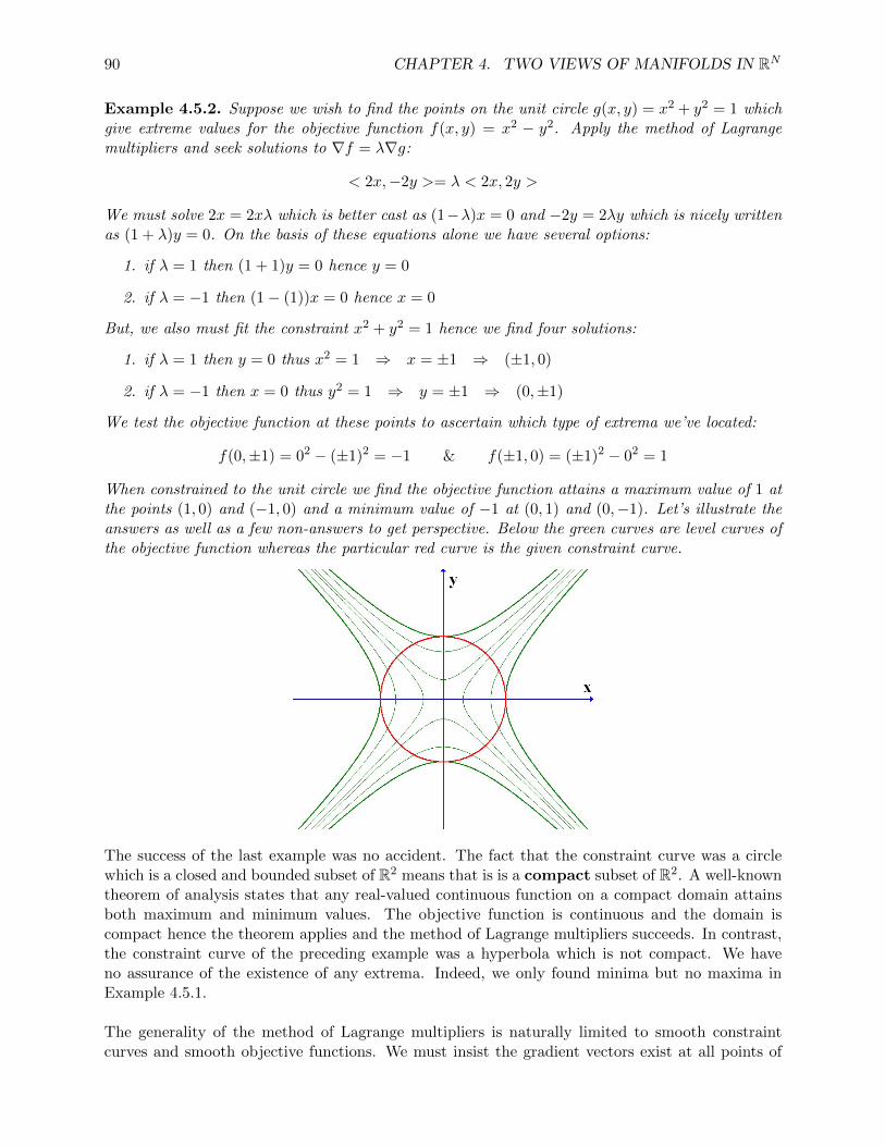
90 CHAPTER 4. TWO VIEWS OF MANIFOLDS IN RN
Example 4.5.2. Suppose we wish to find the points on the unit circle g(x, y) = x2 + y2 = 1 whichgive extreme values for the objective function f(x, y) = x2 − y2. Apply the method of Lagrangemultipliers and seek solutions to ∇f = λ∇g:
< 2x,−2y >= λ < 2x, 2y >
We must solve 2x = 2xλ which is better cast as (1−λ)x = 0 and −2y = 2λy which is nicely writtenas (1 + λ)y = 0. On the basis of these equations alone we have several options:
1. if λ = 1 then (1 + 1)y = 0 hence y = 0
2. if λ = −1 then (1− (1))x = 0 hence x = 0
But, we also must fit the constraint x2 + y2 = 1 hence we find four solutions:
1. if λ = 1 then y = 0 thus x2 = 1 ⇒ x = ±1 ⇒ (±1, 0)
2. if λ = −1 then x = 0 thus y2 = 1 ⇒ y = ±1 ⇒ (0,±1)
We test the objective function at these points to ascertain which type of extrema we’ve located:
f(0,±1) = 02 − (±1)2 = −1 & f(±1, 0) = (±1)2 − 02 = 1
When constrained to the unit circle we find the objective function attains a maximum value of 1 atthe points (1, 0) and (−1, 0) and a minimum value of −1 at (0, 1) and (0,−1). Let’s illustrate theanswers as well as a few non-answers to get perspective. Below the green curves are level curves ofthe objective function whereas the particular red curve is the given constraint curve.
The success of the last example was no accident. The fact that the constraint curve was a circlewhich is a closed and bounded subset of R2 means that is is a compact subset of R2. A well-knowntheorem of analysis states that any real-valued continuous function on a compact domain attainsboth maximum and minimum values. The objective function is continuous and the domain iscompact hence the theorem applies and the method of Lagrange multipliers succeeds. In contrast,the constraint curve of the preceding example was a hyperbola which is not compact. We haveno assurance of the existence of any extrema. Indeed, we only found minima but no maxima inExample 4.5.1.
The generality of the method of Lagrange multipliers is naturally limited to smooth constraintcurves and smooth objective functions. We must insist the gradient vectors exist at all points of
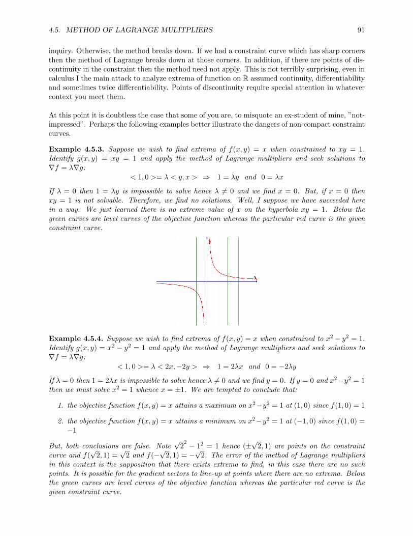
4.5. METHOD OF LAGRANGE MULITPLIERS 91
inquiry. Otherwise, the method breaks down. If we had a constraint curve which has sharp cornersthen the method of Lagrange breaks down at those corners. In addition, if there are points of dis-continuity in the constraint then the method need not apply. This is not terribly surprising, even incalculus I the main attack to analyze extrema of function on R assumed continuity, differentiabilityand sometimes twice differentiability. Points of discontinuity require special attention in whatevercontext you meet them.
At this point it is doubtless the case that some of you are, to misquote an ex-student of mine, ”not-impressed”. Perhaps the following examples better illustrate the dangers of non-compact constraintcurves.
Example 4.5.3. Suppose we wish to find extrema of f(x, y) = x when constrained to xy = 1.Identify g(x, y) = xy = 1 and apply the method of Lagrange multipliers and seek solutions to∇f = λ∇g:
< 1, 0 >= λ < y, x > ⇒ 1 = λy and 0 = λx
If λ = 0 then 1 = λy is impossible to solve hence λ 6= 0 and we find x = 0. But, if x = 0 thenxy = 1 is not solvable. Therefore, we find no solutions. Well, I suppose we have succeeded herein a way. We just learned there is no extreme value of x on the hyperbola xy = 1. Below thegreen curves are level curves of the objective function whereas the particular red curve is the givenconstraint curve.
Example 4.5.4. Suppose we wish to find extrema of f(x, y) = x when constrained to x2 − y2 = 1.Identify g(x, y) = x2 − y2 = 1 and apply the method of Lagrange multipliers and seek solutions to∇f = λ∇g:
< 1, 0 >= λ < 2x,−2y > ⇒ 1 = 2λx and 0 = −2λy
If λ = 0 then 1 = 2λx is impossible to solve hence λ 6= 0 and we find y = 0. If y = 0 and x2−y2 = 1then we must solve x2 = 1 whence x = ±1. We are tempted to conclude that:
1. the objective function f(x, y) = x attains a maximum on x2−y2 = 1 at (1, 0) since f(1, 0) = 1
2. the objective function f(x, y) = x attains a minimum on x2−y2 = 1 at (−1, 0) since f(1, 0) =−1
But, both conclusions are false. Note√
22 − 12 = 1 hence (±
√2, 1) are points on the constraint
curve and f(√
2, 1) =√
2 and f(−√
2, 1) = −√
2. The error of the method of Lagrange multipliersin this context is the supposition that there exists extrema to find, in this case there are no suchpoints. It is possible for the gradient vectors to line-up at points where there are no extrema. Belowthe green curves are level curves of the objective function whereas the particular red curve is thegiven constraint curve.

92 CHAPTER 4. TWO VIEWS OF MANIFOLDS IN RN
Incidentally, if you want additional discussion of Lagrange multipliers for two-dimensional problemsone very nice source I certainly profitted from was the YouTube video by Edward Frenkel of Berkley.See his website http://math.berkeley.edu/ frenkel/ for links.

Chapter 5
critical point analysis for severalvariables
In the typical calculus sequence you learn the first and second derivative tests in calculus I. Thenin calculus II you learn about power series and Taylor’s Theorem. Finally, in calculus III, in manypopular texts, you learn an essentially ad-hoc procedure for judging the nature of critical pointsas minimum, maximum or saddle. These topics are easily seen as disconnected events. In thischapter, we connect them. We learn that the geometry of quadratic forms is ellegantly revealed byeigenvectors and more than that this geometry is precisely what elucidates the proper classificationsof critical points of multivariate functions with real values.
5.1 multivariate power series
We set aside the issue of convergence for now. We will suppose the series discussed in this sectionexist on and converge on some domain, but we do not seek to treat that topic here. Our focus iscomputational. How should we calculate the Taylor series for f(x, y) at (a, b)? Or, what aboutf(x) at xo ∈ Rn?.
5.1.1 taylor’s polynomial for one-variable
If f : U ⊆ R→ R is analytic at xo ∈ U then we can write
f(x) = f(xo) + f ′(xo)(x− xo) +1
2f ′′(xo)(x− xo)2 + · · · =
∞∑n=0
f (n)(xo)
n!(x− xo)n
We could write this in terms of the operator D = ddt and the evaluation of t = xo
f(x) =
[ ∞∑n=0
1
n!(x− t)nDnf(t)
]t=xo
=
I remind the reader that a function is called entire if it is analytic on all of R, for example ex, cos(x)and sin(x) are all entire. In particular, you should know that:
ex = 1 + x+1
2x2 + · · · =
∞∑n=0
1
n!xn
cos(x) = 1− 1
2x2 +
1
4!x4 · · · =
∞∑n=0
(−1)n
(2n)!x2n
93

94 CHAPTER 5. CRITICAL POINT ANALYSIS FOR SEVERAL VARIABLES
sin(x) = x− 1
3!x3 +
1
5!x5 · · · =
∞∑n=0
(−1)n
(2n+ 1)!x2n+1
Since ex = cosh(x) + sinh(x) it also follows that
cosh(x) = 1 +1
2x2 +
1
4!x4 · · · =
∞∑n=0
1
(2n)!x2n
sinh(x) = x+1
3!x3 +
1
5!x5 · · · =
∞∑n=0
1
(2n+ 1)!x2n+1
The geometric series is often useful, for a, r ∈ R with |r| < 1 it is known
a+ ar + ar2 + · · · =∞∑n=0
arn =a
1− r
This generates a whole host of examples, for instance:
1
1 + x2= 1− x2 + x4 − x6 + · · ·
1
1− x3= 1 + x3 + x6 + x9 + · · ·
x3
1− 2x= x3(1 + 2x+ (2x)2 + · · · ) = x3 + 2x4 + 4x5 + · · ·
Moreover, the term-by-term integration and differentiation theorems yield additional results inconjuction with the geometric series:
tan−1(x) =
∫dx
1 + x2=
∫ ∞∑n=0
(−1)nx2ndx =∞∑n=0
(−1)n
2n+ 1x2n+1 = x− 1
3x3 +
1
5x5 + · · ·
ln(1− x) =
∫d
dxln(1− x)dx =
∫−1
1− xdx = −
∫ ∞∑n=0
xndx =∞∑n=0
−1
n+ 1xn+1
Of course, these are just the basic building blocks. We also can twist things and make the studentuse algebra,
ex+2 = exe2 = e2(1 + x+1
2x2 + · · · )
or trigonmetric identities,
sin(x) = sin(x− 2 + 2) = sin(x− 2) cos(2) + cos(x− 2) sin(2)
⇒ sin(x) = cos(2)
∞∑n=0
(−1)n
(2n+ 1)!(x− 2)2n+1 + sin(2)
∞∑n=0
(−1)n
(2n)!(x− 2)2n.
Feel free to peruse my most recent calculus II materials to see a host of similarly sneaky calculations.

5.1. MULTIVARIATE POWER SERIES 95
5.1.2 taylor’s multinomial for two-variables
Suppose we wish to find the taylor polynomial centered at (0, 0) for f(x, y) = ex sin(y). It is asimple as this:
f(x, y) =
(1 + x+
1
2x2 + · · ·
)(y − 1
6y3 + · · ·
)= y + xy +
1
2x2y − 1
6y3 + · · ·
the resulting expression is called a multinomial since it is a polynomial in multiple variables. Ifall functions f(x, y) could be written as f(x, y) = F (x)G(y) then multiplication of series knownfrom calculus II would often suffice. However, many functions do not possess this very specialform. For example, how should we expand f(x, y) = cos(xy) about (0, 0)?. We need to derive thetwo-dimensional Taylor’s theorem.
We already know Taylor’s theorem for functions on R,
g(x) = g(a) + g′(a)(x− a) +1
2g′′(a)(x− a)2 + · · ·+ 1
k!g(k)(a)(x− a)k +Rk
and... If the remainder term vanishes as k → ∞ then the function g is represented by the Taylorseries given above and we write:
g(x) =∞∑k=0
1
k!g(k)(a)(x− a)k.
Consider the function of two variables f : U ⊆ R2 → R which is smooth with smooth partialderivatives of all orders. Furthermore, let (a, b) ∈ U and construct a line through (a, b) withdirection vector (h1, h2) as usual:
φ(t) = (a, b) + t(h1, h2) = (a+ th1, b+ th2)
for t ∈ R. Note φ(0) = (a, b) and φ′(t) = (h1, h2) = φ′(0). Construct g = f ◦φ : R → R andchoose dom(g) such that φ(t) ∈ U for t ∈ dom(g). This function g is a real-valued function of areal variable and we will be able to apply Taylor’s theorem from calculus II on g. However, todifferentiate g we’ll need tools from calculus III to sort out the derivatives. In particular, as wedifferentiate g, note we use the chain rule for functions of several variables:
g′(t) = (f ◦φ)′(t) = f ′(φ(t))φ′(t)
= ∇f(φ(t)) · (h1, h2)= h1fx(a+ th1, b+ th2) + h2fy(a+ th1, b+ th2)
Note g′(0) = h1fx(a, b)+h2fy(a, b). Differentiate again (I omit (φ(t)) dependence in the last steps),
g′′(t) = h1f′x(a+ th1, b+ th2) + h2f
′y(a+ th1, b+ th2)
= h1∇fx(φ(t)) · (h1, h2) + h2∇fy(φ(t)) · (h1, h2)= h21fxx + h1h2fyx + h2h1fxy + h22fyy
= h21fxx + 2h1h2fxy + h22fyy
Thus, making explicit the point dependence, g′′(0) = h21fxx(a, b) + 2h1h2fxy(a, b) + h22fyy(a, b). Wemay construct the Taylor series for g up to quadratic terms:
g(0 + t) = g(0) + tg′(0) +1
2g′′(0) + · · ·
= f(a, b) + t[h1fx(a, b) + h2fy(a, b)] +t2
2
[h21fxx(a, b) + 2h1h2fxy(a, b) + h22fyy(a, b)
]+ · · ·

96 CHAPTER 5. CRITICAL POINT ANALYSIS FOR SEVERAL VARIABLES
Note that g(t) = f(a+ th1, b+ th2) hence g(1) = f(a+ h1, b+ h2) and consequently,
f(a+ h1, b+ h2) = f(a, b) + h1fx(a, b) + h2fy(a, b)+
+1
2
[h21fxx(a, b) + 2h1h2fxy(a, b) + h22fyy(a, b)
]+ · · ·
Omitting point dependence on the 2nd derivatives,
f(a+ h1, b+ h2) = f(a, b) + h1fx(a, b) + h2fy(a, b) + 12
[h21fxx + 2h1h2fxy + h22fyy
]+ · · ·
Sometimes we’d rather have an expansion about (x, y). To obtain that formula simply substitutex − a = h1 and y − b = h2. Note that the point (a, b) is fixed in this discussion so the derivativesare not modified in this substitution,
f(x, y) = f(a, b) + (x− a)fx(a, b) + (y − b)fy(a, b)+
+1
2
[(x− a)2fxx(a, b) + 2(x− a)(y − b)fxy(a, b) + (y − b)2fyy(a, b)
]+ · · ·
At this point we ought to recognize the first three terms give the tangent plane to z = f(z, y) at(a, b, f(a, b)). The higher order terms are nonlinear corrections to the linearization, these quadraticterms form a quadratic form. If we computed third, fourth or higher order terms we will find that,using a = a1 and b = a2 as well as x = x1 and y = x2,
f(x, y) =
∞∑n=0
2∑i1=0
2∑i2=0
· · ·2∑
in=0
1
n!
∂(n)f(a1, a2)
∂xi1∂xi2 · · · ∂xin(xi1 − ai1)(xi2 − ai2) · · · (xin − ain)
Example 5.1.1. Expand f(x, y) = cos(xy) about (0, 0). We calculate derivatives,
fx = −y sin(xy) fy = −x sin(xy)
fxx = −y2 cos(xy) fxy = − sin(xy)− xy cos(xy) fyy = −x2 cos(xy)
fxxx = y3 sin(xy) fxxy = −y cos(xy)− y cos(xy) + xy2 sin(xy)
fxyy = −x cos(xy)− x cos(xy) + x2y sin(xy) fyyy = x3 sin(xy)
Next, evaluate at x = 0 and y = 0 to find f(x, y) = 1 + · · · to third order in x, y about (0, 0). Wecan understand why these derivatives are all zero by approaching the expansion a different route:simply expand cosine directly in the variable (xy),
f(x, y) = 1− 1
2(xy)2 +
1
4!(xy)4 + · · · = 1− 1
2x2y2 +
1
4!x4y4 + · · · .
Apparently the given function only has nontrivial derivatives at (0, 0) at orders 0, 4, 8, .... We candeduce that fxxxxy(0, 0) = 0 without furthter calculation.
This is actually a very interesting function, I think it defies our analysis in the later portion of thischapter. The second order part of the expansion reveals nothing about the nature of the criticalpoint (0, 0). Of course, any student of trigonometry should recognize that f(0, 0) = 1 is likelya local maximum, it’s certainly not a local minimum. The graph reveals that f(0, 0) is a localmaxium for f restricted to certain rays from the origin whereas it is constant on several specialdirections (the coordinate axes).

5.1. MULTIVARIATE POWER SERIES 97
And, if you were wondering, yes, we could also derive this from subsitution of u = xy into thestandard expansion for cos(u) = 1− 1
2u2 + 1
4!u4 + · · · . Often such subsitutions are the quickest way
to generate interesting examples.
5.1.3 taylor’s multinomial for many-variables
Suppose f : dom(f) ⊆ Rn → R is a function of n-variables and we seek to derive the Taylor seriescentered at a = (a1, a2, . . . , an). Once more consider the composition of f with a line in dom(f).In particular, let φ : R → Rn be defined by φ(t) = a + th where h = (h1, h2, . . . , hn) gives thedirection of the line and clearly φ′(t) = h. Let g : dom(g) ⊆ R → R be defined by g(t) = f(φ(t))for all t ∈ R such that φ(t) ∈ dom(f). Differentiate, use the multivariate chain rule, recall herethat ∇ = e1
∂∂x1
+ e2∂∂x2
+ · · ·+ en∂∂xn
=∑n
i=1 ei∂i,
g′(t) = ∇f(φ(t)) · φ′(t) = ∇f(φ(t)) · h =n∑i=1
hi(∂if)(φ(t))
If we omit the explicit dependence on φ(t) then we find the simple formula g′(t) =∑n
i=1 hi∂if .Differentiate a second time,
g′′(t) =d
dt
[ n∑i=1
hi∂if(φ(t))
]=
n∑i=1
hid
dt
[(∂if)(φ(t))
]=
n∑i=1
hi(∇∂if
)(φ(t)) · φ′(t)
Omitting the φ(t) dependence and once more using φ′(t) = h we find
g′′(t) =
n∑i=1
hi∇∂if · h
Recall that ∇ =∑n
j=1 ej∂j and expand the expression above,
g′′(t) =n∑i=1
hi
( n∑j=1
ej∂j∂if
)· h =
n∑i=1
n∑j=1
hihj∂j∂if
where we should remember ∂j∂if depends on φ(t). It should be clear that if we continue and takek-derivatives then we will obtain:
g(k)(t) =n∑
i1=1
n∑i2=1
· · ·n∑
ik=1
hi1hi2 · · ·hik∂i1∂i2 · · · ∂ikf
More explicitly,
g(k)(t) =n∑
i1=1
n∑i2=1
· · ·n∑
ik=1
hi1hi2 · · ·hik(∂i1∂i2 · · · ∂ikf)(φ(t))
98 CHAPTER 5. CRITICAL POINT ANALYSIS FOR SEVERAL VARIABLES
Hence, by Taylor’s theorem, provided we are sufficiently close to t = 0 as to bound the remainder1
g(t) =
∞∑k=0
1
k!
( n∑i1=1
n∑i2=1
· · ·n∑
ik=1
hi1hi2 · · ·hik(∂i1∂i2 · · · ∂ikf)(φ(t))
)tk
Recall that g(t) = f(φ(t)) = f(a+ th). Put2 t = 1 and bring in the 1k! to derive
f(a+ h) =
∞∑k=0
n∑i1=1
n∑i2=1
· · ·n∑
ik=1
1
k!
(∂i1∂i2 · · · ∂ikf
)(a) hi1hi2 · · ·hik .
Naturally, we sometimes prefer to write the series expansion about a as an expresssion in x = a+h.With this substitution we have h = x− a and hij = (x− a)ij = xij − aij thus
f(x) =∞∑k=0
n∑i1=1
n∑i2=1
· · ·n∑
ik=1
1
k!
(∂i1∂i2 · · · ∂ikf
)(a) (xi1 − ai1)(xi2 − ai2) · · · (xik − aik).
Example 5.1.2. Suppose f : R3 → R let’s unravel the Taylor series centered at (0, 0, 0) from thegeneral formula boxed above. Utilize the notation x = x1, y = x2 and z = x3 in this example.
f(x) =∞∑k=0
3∑i1=1
3∑i2=1
· · ·3∑
ik=1
1
k!
(∂i1∂i2 · · · ∂ikf
)(0) xi1xi2 · · ·xik .
The terms to order 2 are as follows:
f(x) = f(0) + fx(0)x+ fy(0)y + fz(0)z
+12
(fxx(0)x2 + fyy(0)y2 + fzz(0)z2+
+fxy(0)xy + fxz(0)xz + fyz(0)yz + fyx(0)yx+ fzx(0)zx+ fzy(0)zy
)+ · · ·
Partial derivatives commute for smooth functions hence,
f(x) = f(0) + fx(0)x+ fy(0)y + fz(0)z
+12
(fxx(0)x2 + fyy(0)y2 + fzz(0)z2 + 2fxy(0)xy + 2fxz(0)xz + 2fyz(0)yz
)+ 1
3!
(fxxx(0)x3 + fyyy(0)y3 + fzzz(0)z3 + 3fxxy(0)x2y + 3fxxz(0)x2z
+3fyyz(0)y2z + 3fxyy(0)xy2 + 3fxzz(0)xz2 + 3fyzz(0)yz2 + 6fxyz(0)xyz
)+ · · ·
1there exist smooth examples for which no neighborhood is small enough, the bump function in one-variable hashigher-dimensional analogues, we focus our attention to functions for which it is possible for the series below toconverge
2if t = 1 is not in the domain of g then we should rescale the vector h so that t = 1 places φ(1) in dom(f), if f issmooth on some neighborhood of a then this is possible

5.2. A BRIEF INTRODUCTION TO THE THEORY OF QUADRATIC FORMS 99
Example 5.1.3. Suppose f(x, y, z) = exyz. Find a quadratic approximation to f near (0, 1, 2).Observe:
fx = yzexyz fy = xzexyz fz = xyexyz
fxx = (yz)2exyz fyy = (xz)2exyz fzz = (xy)2exyz
fxy = zexyz + xyz2exyz fyz = xexyz + x2yzexyz fxz = yexyz + xy2zexyz
Evaluating at x = 0, y = 1 and z = 2,
fx(0, 1, 2) = 2 fy(0, 1, 2) = 0 fz(0, 1, 2) = 0
fxx(0, 1, 2) = 4 fyy(0, 1, 2) = 0 fzz(0, 1, 2) = 0
fxy(0, 1, 2) = 2 fyz(0, 1, 2) = 0 fxz(0, 1, 2) = 1
Hence, as f(0, 1, 2) = e0 = 1 we find
f(x, y, z) = 1 + 2x+ 2x2 + 2x(y − 1) + 2x(z − 2) + · · ·
Another way to calculate this expansion is to make use of the adding zero trick,
f(x, y, z) = ex(y−1+1)(z−2+2) = 1 + x(y − 1 + 1)(z − 2 + 2) +1
2
[x(y − 1 + 1)(z − 2 + 2)
]2+ · · ·
Keeping only terms with two or less of x, (y − 1) and (z − 2) variables,
f(x, y, z) = 1 + 2x+ x(y − 1)(2) + x(1)(z − 2) +1
2x2(1)2(2)2 + · · ·
Which simplifies once more to f(x, y, z) = 1 + 2x+ 2x(y − 1) + x(z − 2) + 2x2 + · · · .
5.2 a brief introduction to the theory of quadratic forms
Definition 5.2.1.
Generally, a quadratic form Q is a function Q : Rn → R whose formula can be writtenQ(~x) = ~xTA~x for all ~x ∈ Rn where A ∈ R n×n such that AT = A. In particular, if ~x = (x, y)
and A =
[a bb c
]then
Q(~x) = ~xTA~x = ax2 + bxy + byx+ cy2 = ax2 + 2bxy + y2.
The n = 3 case is similar,denote A = [Aij ] and ~x = (x, y, z) so that
Q(~x) = ~xTA~x = A11x2 + 2A12xy + 2A13xz +A22y
2 + 2A23yz +A33z2.
Generally, if [Aij ] ∈ R n×n and ~x = [xi]T then the associated quadratic form is
Q(~x) = ~xTA~x =∑i,j
Aijxixj =
n∑i=1
Aiix2i +
∑i<j
2Aijxixj .
In case you wondering, yes you could write a given quadratic form with a different matrix whichis not symmetric, but we will find it convenient to insist that our matrix is symmetric since that

100 CHAPTER 5. CRITICAL POINT ANALYSIS FOR SEVERAL VARIABLES
choice is always possible for a given quadratic form.
It is at times useful to use the dot-product to express a given quadratic form:
~xTA~x = ~x · (A~x) = (A~x) · ~x = ~xTAT~x
Some texts actually use the middle equality above to define a symmetric matrix.
Example 5.2.2.
2x2 + 2xy + 2y2 =[x y
] [ 2 11 2
] [xy
]Example 5.2.3.
2x2 + 2xy + 3xz − 2y2 − z2 =[x y z
] 2 1 3/21 −2 0
3/2 0 −1
xyz
Proposition 5.2.4.
The values of a quadratic form on Rn − {0} is completely determined by it’s values onthe (n − 1)-sphere Sn−1 = {~x ∈ Rn | ||~x|| = 1}. In particular, Q(~x) = ||~x||2Q(x) wherex = 1
||~x||~x.
Proof: Let Q(~x) = ~xTA~x. Notice that we can write any nonzero vector as the product of itsmagnitude ||x|| and its direction x = 1
||~x||~x,
Q(~x) = Q(||~x||x) = (||~x||x)TA||~x||x = ||~x||2xTAx = ||x||2Q(x).
Therefore Q(~x) is simply proportional to Q(x) with proportionality constant ||~x||2. �
The proposition above is very interesting. It says that if we know how Q works on unit-vectors thenwe can extrapolate its action on the remainder of Rn. If f : S → R then we could say f(S) > 0iff f(s) > 0 for all s ∈ S. Likewise, f(S) < 0 iff f(s) < 0 for all s ∈ S. The proposition belowfollows from the proposition above since ||~x||2 ranges over all nonzero positive real numbers in theequations above.
Proposition 5.2.5.
If Q is a quadratic form on Rn and we denote Rn∗ = Rn − {0}
1.(negative definite) Q(Rn∗ ) < 0 iff Q(Sn−1) < 0
2.(positive definite) Q(Rn∗ ) > 0 iff Q(Sn−1) > 0
3.(non-definite) Q(Rn∗ ) = R− {0} iff Q(Sn−1) has both positive and negative values.
Before I get too carried away with the theory let’s look at a couple examples.

5.2. A BRIEF INTRODUCTION TO THE THEORY OF QUADRATIC FORMS 101
Example 5.2.6. Consider the quadric form Q(x, y) = x2 + y2. You can check for yourself thatz = Q(x, y) is a cone and Q has positive outputs for all inputs except (0, 0). Notice that Q(v) = ||v||2so it is clear that Q(S1) = 1. We find agreement with the preceding proposition. Next, think aboutthe application of Q(x, y) to level curves; x2 + y2 = k is simply a circle of radius
√k or just the
origin. Here’s a graph of z = Q(x, y):
Notice that Q(0, 0) = 0 is the absolute minimum for Q. Finally, let’s take a moment to write
Q(x, y) = [x, y]
[1 00 1
] [xy
]in this case the matrix is diagonal and we note that the e-values are
λ1 = λ2 = 1.
Example 5.2.7. Consider the quadric form Q(x, y) = x2 − 2y2. You can check for yourselfthat z = Q(x, y) is a hyperboloid and Q has non-definite outputs since sometimes the x2 termdominates whereas other points have −2y2 as the dominent term. Notice that Q(1, 0) = 1 whereasQ(0, 1) = −2 hence we find Q(S1) contains both positive and negative values and consequently wefind agreement with the preceding proposition. Next, think about the application of Q(x, y) to levelcurves; x2 − 2y2 = k yields either hyperbolas which open vertically (k > 0) or horizontally (k < 0)or a pair of lines y = ±x
2 in the k = 0 case. Here’s a graph of z = Q(x, y):
The origin is a saddle point. Finally, let’s take a moment to write Q(x, y) = [x, y]
[1 00 −2
] [xy
]in this case the matrix is diagonal and we note that the e-values are λ1 = 1 and λ2 = −2.

102 CHAPTER 5. CRITICAL POINT ANALYSIS FOR SEVERAL VARIABLES
Example 5.2.8. Consider the quadric form Q(x, y) = 3x2. You can check for yourself that z =Q(x, y) is parabola-shaped trough along the y-axis. In this case Q has positive outputs for all inputsexcept (0, y), we would call this form positive semi-definite. A short calculation reveals thatQ(S1) = [0, 3] thus we again find agreement with the preceding proposition (case 3). Next, thinkabout the application of Q(x, y) to level curves; 3x2 = k is a pair of vertical lines: x = ±
√k/3 or
just the y-axis. Here’s a graph of z = Q(x, y):
Finally, let’s take a moment to write Q(x, y) = [x, y]
[3 00 0
] [xy
]in this case the matrix is
diagonal and we note that the e-values are λ1 = 3 and λ2 = 0.
Example 5.2.9. Consider the quadric form Q(x, y, z) = x2+2y2+3z2. Think about the applicationof Q(x, y, z) to level surfaces; x2 + 2y2 + 3z2 = k is an ellipsoid. I can’t graph a function of threevariables, however, we can look at level surfaces of the function. I use Mathematica to plot severalbelow:
Finally, let’s take a moment to write Q(x, y, z) = [x, y, z]
1 0 00 2 00 0 3
xyz
in this case the matrix
is diagonal and we note that the e-values are λ1 = 1 and λ2 = 2 and λ3 = 3.
5.2.1 diagonalizing forms via eigenvectors
The examples given thus far are the simplest cases. We don’t really need linear algebra to un-derstand them. In contrast, e-vectors and e-values will prove a useful tool to unravel the laterexamples3
3this is the one place in this course where we need eigenvalues and eigenvector calculations, I include these toillustrate the structure of quadratic forms in general, however, as linear algebra is not a prerequisite you may find somethings in this section mysterious. The homework and study guide will elaborate on what is required this semester

5.2. A BRIEF INTRODUCTION TO THE THEORY OF QUADRATIC FORMS 103
Definition 5.2.10.
Let A ∈ R n×n. If v ∈ R n×1 is nonzero and Av = λv for some λ ∈ C then we say v is aneigenvector with eigenvalue λ of the matrix A.
Proposition 5.2.11.
Let A ∈ R n×n then λ is an eigenvalue of A iff det(A−λI) = 0. We say P (λ) = det(A−λI)the characteristic polynomial and det(A− λI) = 0 is the characteristic equation.
Proof: Suppose λ is an eigenvalue of A then there exists a nonzero vector v such that Av = λvwhich is equivalent to Av − λv = 0 which is precisely (A − λI)v = 0. Notice that (A − λI)0 = 0thus the matrix (A − λI) is singular as the equation (A − λI)x = 0 has more than one solution.Consequently det(A− λI) = 0.
Conversely, suppose det(A − λI) = 0. It follows that (A − λI) is singular. Clearly the system(A − λI)x = 0 is consistent as x = 0 is a solution hence we know there are infinitely many solu-tions. In particular there exists at least one vector v 6= 0 such that (A−λI)v = 0 which means thevector v satisfies Av = λv. Thus v is an eigenvector with eigenvalue λ for A. �
Remark 5.2.12.
I found a pretty derivation of the eigenvector condition from the method of Lagrange mul-tipliers. I shared in the Lecture 10 part 1. It’s likely I cover that argument again in Lecturethis year, my apologies it has not made it to these notes at this time.
Example 5.2.13. Let A =
[3 13 1
]find the e-values and e-vectors of A.
det(A− λI) = det
[3− λ 1
3 1− λ
]= (3− λ)(1− λ)− 3 = λ2 − 4λ = λ(λ− 4) = 0
We find λ1 = 0 and λ2 = 4. Now find the e-vector with e-value λ1 = 0, let u1 = [u, v]T denote thee-vector we wish to find. Calculate,
(A− 0I)u1 =
[3 13 1
] [uv
]=
[3u+ v3u+ v
]=
[00
]Obviously the equations above are redundant and we have infinitely many solutions of the form
3u+ v = 0 which means v = −3u so we can write, u1 =
[u−3u
]= u
[1−3
]. In applications we
often make a choice to select a particular e-vector. Most modern graphing calculators can calcu-late e-vectors. It is customary for the e-vectors to be chosen to have length one. That is a usefulchoice for certain applications as we will later discuss. If you use a calculator it would likely give
u1 = 1√10
[1−3
]although the
√10 would likely be approximated unless your calculator is smart.
Continuing we wish to find eigenvectors u2 = [u, v]T such that (A − 4I)u2 = 0. Notice that u, vare disposable variables in this context, I do not mean to connect the formulas from the λ = 0 casewith the case considered now.
(A− 4I)u1 =
[−1 13 −3
] [uv
]=
[−u+ v3u− 3v
]=
[00
]

104 CHAPTER 5. CRITICAL POINT ANALYSIS FOR SEVERAL VARIABLES
Again the equations are redundant and we have infinitely many solutions of the form v = u. Hence,
u2 =
[uu
]= u
[11
]is an eigenvector for any u ∈ R such that u 6= 0.
Theorem 5.2.14.
A matrix A ∈ R n×n is symmetric iff there exists an orthonormal eigenbasis for A.
There is a geometric proof of this theorem in Edwards4 (see Theorem 8.6 pgs 146-147) . I prove halfof this theorem in my linear algebra notes by a non-geometric argument (full proof is in Appendix Cof Insel,Spence and Friedberg). It might be very interesting to understand the connection betweenthe geometric verse algebraic arguments. We’ll content ourselves with an example here:
Example 5.2.15. Let A =
0 0 00 1 20 2 1
. Observe that det(A− λI) = −λ(λ+ 1)(λ− 3) thus λ1 =
0, λ2 = −1, λ3 = 3. We can calculate orthonormal e-vectors of v1 = [1, 0, 0]T , v2 = 1√2[0, 1,−1]T
and v3 = 1√2[0, 1, 1]T . I invite the reader to check the validity of the following equation: 1 0 0
0 1√2−1√2
0 1√2
1√2
0 0 0
0 1 20 2 1
1 0 0
0 1√2
1√2
0 −1√2
1√2
=
0 0 00 −1 00 0 3
Its really neat that to find the inverse of a matrix of orthonormal e-vectors we need only take thetranspose; note 1 0 0
0 1√2−1√2
0 1√2
1√2
1 0 0
0 1√2
1√2
0 −1√2
1√2
=
1 0 00 1 00 0 1
.Proposition 5.2.16.
If Q is a quadratic form on Rn with matrix A and e-values λ1, λ2, . . . , λn with orthonormale-vectors v1, v2, . . . , vn then
Q(vi) = λi2
for i = 1, 2, . . . , n. Moreover, if P = [v1|v2| · · · |vn] then
Q(~x) = (P T~x)TP TAPP T~x = λ1y21 + λ2y
22 + · · ·+ λny
2n
where we defined ~y = P T~x.
Let me restate the proposition above in simple terms: we can transform a given quadratic form toa diagonal form by finding orthonormalized e-vectors and performing the appropriate coordinatetransformation. Since P is formed from orthonormal e-vectors we know that P will be either arotation or reflection. This proposition says we can remove ”cross-terms” by transforming thequadratic forms with an appropriate rotation.
4think about it, there is a 1-1 correspondance between symmetric matrices and quadratic forms
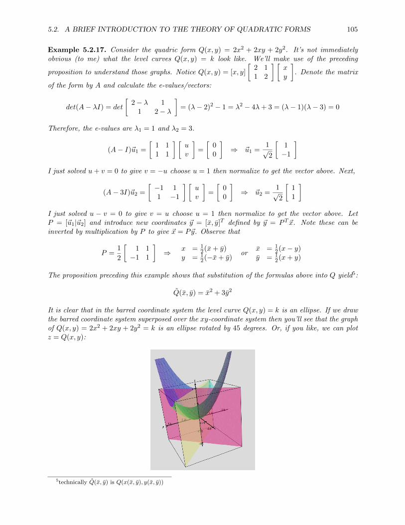
5.2. A BRIEF INTRODUCTION TO THE THEORY OF QUADRATIC FORMS 105
Example 5.2.17. Consider the quadric form Q(x, y) = 2x2 + 2xy + 2y2. It’s not immediatelyobvious (to me) what the level curves Q(x, y) = k look like. We’ll make use of the preceding
proposition to understand those graphs. Notice Q(x, y) = [x, y]
[2 11 2
] [xy
]. Denote the matrix
of the form by A and calculate the e-values/vectors:
det(A− λI) = det
[2− λ 1
1 2− λ
]= (λ− 2)2 − 1 = λ2 − 4λ+ 3 = (λ− 1)(λ− 3) = 0
Therefore, the e-values are λ1 = 1 and λ2 = 3.
(A− I)~u1 =
[1 11 1
] [uv
]=
[00
]⇒ ~u1 =
1√2
[1−1
]I just solved u+ v = 0 to give v = −u choose u = 1 then normalize to get the vector above. Next,
(A− 3I)~u2 =
[−1 11 −1
] [uv
]=
[00
]⇒ ~u2 =
1√2
[11
]I just solved u − v = 0 to give v = u choose u = 1 then normalize to get the vector above. LetP = [~u1|~u2] and introduce new coordinates ~y = [x, y]T defined by ~y = P T~x. Note these can beinverted by multiplication by P to give ~x = P~y. Observe that
P =1
2
[1 1−1 1
]⇒ x = 1
2(x+ y)y = 1
2(−x+ y)or
x = 12(x− y)
y = 12(x+ y)
The proposition preceding this example shows that substitution of the formulas above into Q yield5:
Q(x, y) = x2 + 3y2
It is clear that in the barred coordinate system the level curve Q(x, y) = k is an ellipse. If we drawthe barred coordinate system superposed over the xy-coordinate system then you’ll see that the graphof Q(x, y) = 2x2 + 2xy + 2y2 = k is an ellipse rotated by 45 degrees. Or, if you like, we can plotz = Q(x, y):
5technically Q(x, y) is Q(x(x, y), y(x, y))

106 CHAPTER 5. CRITICAL POINT ANALYSIS FOR SEVERAL VARIABLES
Example 5.2.18. Consider the quadric form Q(x, y) = x2+2xy+y2. It’s not immediately obvious(to me) what the level curves Q(x, y) = k look like. We’ll make use of the preceding proposition to
understand those graphs. Notice Q(x, y) = [x, y]
[1 11 1
] [xy
]. Denote the matrix of the form by
A and calculate the e-values/vectors:
det(A− λI) = det
[1− λ 1
1 1− λ
]= (λ− 1)2 − 1 = λ2 − 2λ = λ(λ− 2) = 0
Therefore, the e-values are λ1 = 0 and λ2 = 2.
(A− 0)~u1 =
[1 11 1
] [uv
]=
[00
]⇒ ~u1 =
1√2
[1−1
]I just solved u+ v = 0 to give v = −u choose u = 1 then normalize to get the vector above. Next,
(A− 2I)~u2 =
[−1 11 −1
] [uv
]=
[00
]⇒ ~u2 =
1√2
[11
]I just solved u − v = 0 to give v = u choose u = 1 then normalize to get the vector above. LetP = [~u1|~u2] and introduce new coordinates ~y = [x, y]T defined by ~y = P T~x. Note these can beinverted by multiplication by P to give ~x = P~y. Observe that
P =1
2
[1 1−1 1
]⇒ x = 1
2(x+ y)y = 1
2(−x+ y)or
x = 12(x− y)
y = 12(x+ y)
The proposition preceding this example shows that substitution of the formulas above into Q yield:
Q(x, y) = 2y2
It is clear that in the barred coordinate system the level curve Q(x, y) = k is a pair of paralelllines. If we draw the barred coordinate system superposed over the xy-coordinate system then you’llsee that the graph of Q(x, y) = x2 + 2xy + y2 = k is a line with slope −1. Indeed, with a littlealgebraic insight we could have anticipated this result since Q(x, y) = (x+y)2 so Q(x, y) = k impliesx+ y =
√k thus y =
√k − x. Here’s a plot which again verifies what we’ve already found:

5.2. A BRIEF INTRODUCTION TO THE THEORY OF QUADRATIC FORMS 107
Example 5.2.19. Consider the quadric form Q(x, y) = 4xy. It’s not immediately obvious (tome) what the level curves Q(x, y) = k look like. We’ll make use of the preceding proposition to
understand those graphs. Notice Q(x, y) = [x, y]
[0 20 2
] [xy
]. Denote the matrix of the form by
A and calculate the e-values/vectors:
det(A− λI) = det
[−λ 22 −λ
]= λ2 − 4 = (λ+ 2)(λ− 2) = 0
Therefore, the e-values are λ1 = −2 and λ2 = 2.
(A+ 2I)~u1 =
[2 22 2
] [uv
]=
[00
]⇒ ~u1 =
1√2
[1−1
]I just solved u+ v = 0 to give v = −u choose u = 1 then normalize to get the vector above. Next,
(A− 2I)~u2 =
[−2 22 −2
] [uv
]=
[00
]⇒ ~u2 =
1√2
[11
]I just solved u − v = 0 to give v = u choose u = 1 then normalize to get the vector above. LetP = [~u1|~u2] and introduce new coordinates ~y = [x, y]T defined by ~y = P T~x. Note these can beinverted by multiplication by P to give ~x = P~y. Observe that
P =1
2
[1 1−1 1
]⇒ x = 1
2(x+ y)y = 1
2(−x+ y)or
x = 12(x− y)
y = 12(x+ y)
The proposition preceding this example shows that substitution of the formulas above into Q yield:
Q(x, y) = −2x2 + 2y2
It is clear that in the barred coordinate system the level curve Q(x, y) = k is a hyperbola. If wedraw the barred coordinate system superposed over the xy-coordinate system then you’ll see thatthe graph of Q(x, y) = 4xy = k is a hyperbola rotated by 45 degrees. The graph z = 4xy is thus ahyperbolic paraboloid:
The fascinating thing about the mathematics here is that if you don’t want to graph z = Q(x, y),but you do want to know the general shape then you can determine which type of quadraic surfaceyou’re dealing with by simply calculating the eigenvalues of the form.

108 CHAPTER 5. CRITICAL POINT ANALYSIS FOR SEVERAL VARIABLES
Remark 5.2.20.
I made the preceding triple of examples all involved the same rotation. This is purely for mylecturing convenience. In practice the rotation could be by all sorts of angles. In addition,you might notice that a different ordering of the e-values would result in a redefinition ofthe barred coordinates. 6
We ought to do at least one 3-dimensional example.
Example 5.2.21. Consider the quadric form Q defined below:
Q(x, y, z) = [x, y, z]
6 −2 0−2 6 0
0 0 5
xyz
Denote the matrix of the form by A and calculate the e-values/vectors:
det(A− λI) = det
6− λ −2 0−2 6− λ 00 0 5− λ
= [(λ− 6)2 − 4](5− λ)
= (5− λ)[λ2 − 12λ+ 32](5− λ)
= (λ− 4)(λ− 8)(5− λ)
Therefore, the e-values are λ1 = 4, λ2 = 8 and λ3 = 5. After some calculation we find the followingorthonormal e-vectors for A:
~u1 =1√2
110
~u2 =1√2
1−10
~u3 =
001
Let P = [~u1|~u2|~u3] and introduce new coordinates ~y = [x, y, z]T defined by ~y = P T~x. Note thesecan be inverted by multiplication by P to give ~x = P~y. Observe that
P =1√2
1 1 0−1 1 0
0 0√
2
⇒x = 1
2(x+ y)y = 1
2(−x+ y)z = z
orx = 1
2(x− y)y = 1
2(x+ y)z = z
The proposition preceding this example shows that substitution of the formulas above into Q yield:
Q(x, y, z) = 4x2 + 8y2 + 5z2
It is clear that in the barred coordinate system the level surface Q(x, y, z) = k is an ellipsoid. If wedraw the barred coordinate system superposed over the xyz-coordinate system then you’ll see thatthe graph of Q(x, y, z) = k is an ellipsoid rotated by 45 degrees around the z − axis. Plotted beloware a few representative ellipsoids:

5.3. SECOND DERIVATIVE TEST IN MANY-VARIABLES 109
In summary, the behaviour of a quadratic form Q(x) = xTAx is governed by it’s set of eigenvalues7
{λ1, λ2, . . . , λk}. Moreover, the form can be written as Q(y) = λ1y21 +λ2y
22 + · · ·+λky
2k by choosing
the coordinate system which is built from the orthonormal eigenbasis of col(A). In this coordinatesystem the shape of the level-sets of Q becomes manifest from the signs of the e-values. )
Remark 5.2.22.
If you would like to read more about conic sections or quadric surfaces and their connectionto e-values/vectors I reccommend sections 9.6 and 9.7 of Anton’s linear algebra text. Ihave yet to add examples on how to include translations in the analysis. It’s not muchmore trouble but I decided it would just be an unecessary complication this semester.Also, section 7.1,7.2 and 7.3 in Lay’s linear algebra text show a bit more about how touse this math to solve concrete applied problems. You might also take a look in GilbertStrang’s linear algebra text, his discussion of tests for positive-definite matrices is muchmore complete than I will give here.
5.3 second derivative test in many-variables
There is a connection between the shape of level curves Q(x1, x2, . . . , xn) = k and the graph xn+1 =f(x1, x2, . . . , xn) of f . I’ll discuss n = 2 but these comments equally well apply to w = f(x, y, z) orhigher dimensional examples. Consider a critical point (a, b) for f(x, y) then the Taylor expansionabout (a, b) has the form
f(a+ h, b+ k) = f(a, b) +Q(h, k)
where Q(h, k) = 12h
2fxx(a, b) +hkfxy(a, b) + 12h
2fyy(a, b) = [h, k][Q](h, k). Since [Q]T = [Q] we canfind orthonormal e-vectors ~u1, ~u2 for [Q] with e-values λ1 and λ2 respective. Using U = [~u1|~u2] wecan introduce rotated coordinates (h, k) = U(h, k). These will give
Q(h, k) = λ1h2 + λ2k
2
Clearly if λ1 > 0 and λ2 > 0 then f(a, b) yields the local minimum whereas if λ1 < 0 and λ2 < 0then f(a, b) yields the local maximum. Edwards discusses these matters on pgs. 148-153. In short,supposing f ≈ f(p) + Q, if all the e-values of Q are positive then f has a local minimum of f(p)at p whereas if all the e-values of Q are negative then f reaches a local maximum of f(p) at p.Otherwise Q has both positive and negative e-values and we say Q is non-definite and the functionhas a saddle point. If all the e-values of Q are positive then Q is said to be positive-definitewhereas if all the e-values of Q are negative then Q is said to be negative-definite. Edwardsgives a few nice tests for ascertaining if a matrix is positive definite without explicit computationof e-values. Finally, if one of the e-values is zero then the graph will be like a trough.
7this set is called the spectrum of the matrix

110 CHAPTER 5. CRITICAL POINT ANALYSIS FOR SEVERAL VARIABLES
Example 5.3.1. Suppose f(x, y) = exp(−x2 − y2 + 2y − 1) expand f about the point (0, 1):
f(x, y) = exp(−x2)exp(−y2 + 2y − 1) = exp(−x2)exp(−(y − 1)2)
expanding,
f(x, y) = (1− x2 + · · · )(1− (y − 1)2 + · · · ) = 1− x2 − (y − 1)2 + · · ·
Recenter about the point (0, 1) by setting x = h and y = 1 + k so
f(h, 1 + k) = 1− h2 − k2 + · · ·
If (h, k) is near (0, 0) then the dominant terms are simply those we’ve written above hence the graphis like that of a quadraic surface with a pair of negative e-values. It follows that f(0, 1) is a localmaximum. In fact, it happens to be a global maximum for this function.
Example 5.3.2. Suppose f(x, y) = 4−(x−1)2+(y−2)2+Aexp(−(x−1)2−(y−2)2)+2B(x−1)(y−2)for some constants A,B. Analyze what values for A,B will make (1, 2) a local maximum, minimumor neither. Expanding about (1, 2) we set x = 1 + h and y = 2 + k in order to see clearly the localbehaviour of f at (1, 2),
f(1 + h, 2 + k) = 4− h2 − k2 +Aexp(−h2 − k2) + 2Bhk= 4− h2 − k2 +A(1− h2 − k2) + 2Bhk · · ·= 4 +A− (A+ 1)h2 + 2Bhk − (A+ 1)k2 + · · ·
There is no nonzero linear term in the expansion at (1, 2) which indicates that f(1, 2) = 4 + Amay be a local extremum. In this case the quadratic terms are nontrivial which means the graph ofthis function is well-approximated by a quadraic surface near (1, 2). The quadratic form Q(h, k) =−(A+ 1)h2 + 2Bhk − (A+ 1)k2 has matrix
[Q] =
[−(A+ 1) B
B −(A+ 1)2
].
The characteristic equation for Q is
det([Q]− λI) = det
[−(A+ 1)− λ B
B −(A+ 1)2 − λ
]= (λ+A+ 1)2 −B2 = 0
We find solutions λ1 = −A− 1 +B and λ2 = −A− 1−B. The possibilities break down as follows:
1. if λ1, λ2 > 0 then f(1, 2) is local minimum.
2. if λ1, λ2 < 0 then f(1, 2) is local maximum.
3. if just one of λ1, λ2 is zero then f is constant along one direction and min/max along anotherso technically it is a local extremum.
4. if λ1λ2 < 0 then f(1, 2) is not a local etremum, however it is a saddle point.
In particular, the following choices for A,B will match the choices above
1. Let A = −3 and B = 1 so λ1 = 3 and λ2 = 1;
2. Let A = 3 and B = 1 so λ1 = −3 and λ2 = −5

5.3. SECOND DERIVATIVE TEST IN MANY-VARIABLES 111
3. Let A = −3 and B = −2 so λ1 = 0 and λ2 = 4
4. Let A = 1 and B = 3 so λ1 = 1 and λ2 = −5
Here are the graphs of the cases above, note the analysis for case 3 is more subtle for Taylorapproximations as opposed to simple quadraic surfaces. In this example, case 3 was also a localminimum. In contrast, in Example 5.2.18 the graph was like a trough. The behaviour of f awayfrom the critical point includes higher order terms whose influence turns the trough into a localminimum.
Example 5.3.3. Suppose f(x, y) = sin(x) cos(y) to find the Taylor series centered at (0, 0) we cansimply multiply the one-dimensional result sin(x) = x− 1
3!x3 + 1
5!x5 + · · · and cos(y) = 1− 1
2!y2 +
14!y
4 + · · · as follows:
f(x, y) = (x− 13!x
3 + 15!x
5 + · · · )(1− 12!y
2 + 14!y
4 + · · · )= x− 1
2xy2 + 1
24xy4 − 1
6x3 − 1
12x3y2 + · · ·
= x+ · · ·
The origin (0, 0) is a critical point since fx(0, 0) = 0 and fy(0, 0) = 0, however, this particularcritical point escapes the analysis via the quadratic form term since Q = 0 in the Taylor seriesfor this function at (0, 0). This is analogous to the inconclusive case of the 2nd derivative test incalculus III.
Example 5.3.4. Suppose f(x, y, z) = xyz. Calculate the multivariate Taylor expansion about thepoint (1, 2, 3). I’ll actually calculate this one via differentiation, I have used tricks and/or calculusII results to shortcut any differentiation in the previous examples. Calculate first derivatives
fx = yz fy = xz fz = xy,
and second derivatives,fxx = 0 fxy = z fxz = y
fyx = z fyy = 0 fyz = x
fzx = y fzy = x fzz = 0,
and the nonzero third derivatives,
fxyz = fyzx = fzxy = fzyx = fyxz = fxzy = 1.
It follows,
f(a+ h, b+ k, c+ l) == f(a, b, c) + fx(a, b, c)h + fy(a, b, c)k + fz(a, b, c)l +
12( fxxhh+ fxyhk + fxzhl + fyxkh+ fyykk + fyzkl + fzxlh+ fzylk + fzzll ) + · · ·

112 CHAPTER 5. CRITICAL POINT ANALYSIS FOR SEVERAL VARIABLES
Of course certain terms can be combined since fxy = fyx etc... for smooth functions (we assumesmooth in this section, moreover the given function here is clearly smooth). In total,
f(1 + h, 2 + k, 3 + l) = 6 + 6h+ 3k + 2l +1
2
(3hk + 2hl + 3kh+ kl + 2lh+ lk
)+
1
3!(6)hkl
Of course, we could also obtain this from simple algebra:
f(1 + h, 2 + k, 3 + l) = (1 + h)(2 + k)(3 + l) = 6 + 6h+ 3k + l + 3hk + 2hl + kl + hkl.

Chapter 6
introduction to variational calculus
6.1 history
The problem of variational calculus is almost as old as modern calculus. Variational calculus seeksto answer questions such as:
Remark 6.1.1.
1. what is the shortest path between two points on a surface ?
2. what is the path of least time for a mass sliding without friction down some pathbetween two given points ?
3. what is the path which minimizes the energy for some physical system ?
4. given two points on the x-axis and a particular area what curve has the longestperimeter and bounds that area between those points and the x-axis?
You’ll notice these all involve a variable which is not a real variable or even a vector-valued-variable.Instead, the answers to the questions posed above will be paths or curves depending on how youwish to frame the problem. In variational calculus the variable is a function and we wish to findextreme values for a functional. In short, a functional is an abstract function of functions. Afunctional takes as an input a function and gives as an output a number. The space from whichthese functions are taken varies from problem to problem. Often we put additional contraintsor conditions on the space of admissable solutions. To read about the full generality of theproblem you should look in a text such as Hans Sagan’s. Our treatment is introductory in this chap-ter, my aim is to show you why it is plausible and then to show you how we use variational calculus.
We will see that the problem of finding an extreme value for a functional is equivalent to solvingthe Euler-Lagrange equations or Euler equations for the functional. Euler predates Lagrange in hisdiscovery of the equations bearing their names. Eulers’s initial attack of the problem was to chopthe hypothetical solution curve up into a polygonal path. The unknowns in that approach werethe coordinates of the vertices in the polygonal path. Then through some ingenious calculationshe arrived at the Euler-Lagrange equations. Apparently there were logical flaws in Euler’s origi-nal treatment. Lagrange later derived the same equations using the viewpoint that the variablewas a function and the variation was one of shifting by an arbitrary function. The treatment of
113
114 CHAPTER 6. INTRODUCTION TO VARIATIONAL CALCULUS
variational calculus in Edwards is neither Euler nor Lagrange’s approach, it is a refined versionwhich takes in the contributions of generations of mathematicians working on the subject and thenmerges it with careful functional analysis. I’m no expert of the full history, I just give you a roughsketch of what I’ve gathered from reading a few variational calculus texts.
Physics played a large role in the development of variational calculus. Lagrange was a physicistas well as a mathematician. At the present time, every physicist takes course(s) in LagrangianMechanics. Moreover, the use of variational calculus is fundamental since Hamilton’s principle saysthat all physics can be derived from the principle of least action. In short this means that nature islazy. The solutions realized in the physical world are those which minimize the action. The action
S[y] =
∫L(y, y′, t) dt
is constructed from the Lagrangian L = T −U where T is the kinetic energy and U is the potentialenergy. In the case of classical mechanics the Euler Lagrange equations are precisely Newton’sequations. The Hamiltonian H = T + U is similar to the Lagrangian except that the fundamentalvariables are taken to be momentum and position in contrast to velocity and position in Lagrangianmechanics.
Hamiltonians and Lagrangians are used to set-up new physical theories. Euler-Lagrange equationsare said to give the so-called classical limit of modern field theories. The concept of a force is notso useful to quantum theories, instead the concept of energy plays the central role. Moreover, theproblem of quantizing and then renormalizing field theory brings in very sophisiticated mathemat-ics. In fact, the math of modern physics is not understood. In this chapter I’ll just show you afew famous classical mechanics problems which are beatifully solved by Lagrange’s approach. We’llalso see how expressing the Lagrangian in non-Cartesian coordinates can give us an easy way toderive forces that arise from geometric contraints.
I am following the typical physics approach to variational calculus. Edwards’ last chapter is morenatural mathematically but I think the math is a bit much for your first exposure to the subject.The treatment given here is close to that of Arfken and Weber’s Mathematical Physics text, how-ever I suspect you can find these calculations in dozens of classical mechanics texts. More or lessour approach is that of Lagrange.
6.2 the variational problem
Our goal in what follows here is to maximize or minimize a particular function of functions. SupposeFo is a set of functions with some particular property. For now, we may could assume that all thefunctions in Fo have graphs that include (x1, y1) and (x2, y2). Consider a functional J : Fo → Fowhich is defined by an integral of some function f which we call the Lagrangian,
J [y] =
∫ x2
x1
f(y, y′, x) dx.
We suppose that f is given but y is a variable. Consider that if we are given a function y∗ ∈ Foand another function η such that η(x1) = η(x2) = 0 then we can reach a whole family of functionsindexed by a real variable α as follows (relabel y∗(x) by y(x, 0) so it matches the rest of the familyof functions):
y(x, α) = y(x, 0) + αη(x)
6.2. THE VARIATIONAL PROBLEM 115
Note that x 7→ y(x, α) gives a function in Fo. We define the variation of y to be
δy = αη(x)
This means y(x, α) = y(x, 0) + δy. We may write J as a function of α given the variation we justdescribed:
J(α) =
∫ x2
x1
f(y(x, α), y(x, α)′, x) dx.
It is intuitively obvious that if the function y∗(x) = y(x, 0) is an extremum of the functional thenwe ought to expect [
∂J(α)
∂α
]α=0
= 0
Notice that we can calculate the derivative above using multivariate calculus. Remember thaty(x, α) = y(x, 0) + αη(x) hence y(x, α)′ = y(x, 0)′ + αη(x)′ thus ∂y
∂α = η and ∂y′
∂α = η′ = dηdx .
Consider that:
∂J(α)
∂α=
∂
∂α
[ ∫ x2
x1
f(y(x, α), y(x, α)′, x) dx
]=
∫ x2
x1
(∂f
∂y
∂y
∂α+∂f
∂y′∂y′
∂α+∂f
∂x
∂x
∂α
)dx
=
∫ x2
x1
(∂f
∂yη +
∂f
∂y′dη
dx
)dx (6.1)
Observe thatd
dx
[∂f
∂y′η
]=
d
dx
[∂f
∂y′
]η +
∂f
∂y′dη
dx
Hence continuing Equation 6.1 in view of the product rule above,
∂J(α)
∂α=
∫ x2
x1
(∂f
∂yη +
d
dx
[∂f
∂y′η
]− d
dx
[∂f
∂y′
]η
)dx
=∂f
∂y′η
∣∣∣∣x2x1
+
∫ x2
x1
(∂f
∂yη − d
dx
[∂f
∂y′
]η
)dx (6.2)
=
∫ x2
x1
(∂f
∂y− d
dx
[∂f
∂y′
] )η dx
Note we used the conditions η(x1) = η(x2) to see that ∂f∂y′ η
∣∣x2x1
= ∂f∂y′ η(x2)− ∂f
∂y′ η(x1) = 0. Our goalis to find the extreme values for the functional J . Let me take a few sentences to again restateour set-up. Generally, we take a function y then J maps to a new function J [y]. The family offunctions indexed by α gives a whole ensemble of functions in Fo which are near y∗ according tothe formula,
y(x, α) = y∗(x) + αη(x)
Let’s call this set of functions Wη. If we took another function like η, say ζ such that ζ(x1) =ζ(x2) = 0 then we could look at another family of functions:
y(x, α) = y∗(x) + αζ(x)
and we could denote the set of all such functions generated from ζ to be Wζ . The total variationof y based at y∗ should include all possible families of functions in Fo. You could think of Wη andWζ be two different subspaces in Fo. If η 6= ζ then these subspaces of Fo are likely disjoint except

116 CHAPTER 6. INTRODUCTION TO VARIATIONAL CALCULUS
for the proposed extremal solution y∗. It is perhaps a bit unsettling to realize there are infinitelymany such subspaces because there are infinitely many choices for the function η or ζ. In any event,
each possible variation of y∗ must satisfy the condition
[∂J(α)∂α
]α=0
= 0 since we assume that y∗
is an extreme value of the functional J . It follows that the Equation 6.2 holds for all possible η.Therefore, we ought to expect that any extreme value of the functional J [y] =
∫ x2x1f(y, y′, x) dx
must solve the Euler Lagrange Equations:
∂f
∂y− d
dx
[∂f
∂y′
]= 0 Euler-Lagrange Equations for J [y] =
∫ x2
x1
f(y, y′, x) dx
6.3 variational derivative
The role that η played in the discussion in the preceding section is somewhat similar to the rolethat the ”h” plays in the definition f ′(a) = limh→0
f(a+h)−f(a)h . You might hope we could replace
arguments in η with a more direct approach. Physicists have a heuristic way of making sucharguments in terms of the variation δ. They would cast the arguments in the last page by just”taking the variation of J”. Let me give you their formal argument,
δJ = δ
[ ∫ x2
x1
f(y, y′, x) dx
]=
[ ∫ x2
x1
δf(y, y′, x) dx
]=
∫ x2
x1
(∂f
∂yδy +
∂f
∂y′δ( dydx
)+∂f
∂xδx
)dx
=
∫ x2
x1
(∂f
∂yδy +
∂f
∂y′d
dx
(δy) )
dx (6.3)
=∂f
∂y′δy
∣∣∣∣x2x1
+
∫ x2
x1
(∂f
∂y− d
dx
[∂f
∂y′
] )δy dx
Therefore, since δy = 0 at the endpoints of integration, the Euler-Lagrange equations follow fromδJ = 0. Now, if you’re like me, the argument above is less than satisfying since we never actuallydefined what it means to ”take δ” of something. Also, why could I commute the variational δ andddx )? That said, the formal method is not without use since it allows the focus to be on the EulerLagrange equations rather than the technical details of the variation.
Remark 6.3.1.
The more adept reader at this point should realize the hypocrisy of me calling the abovecalculation formal since even my presentation here was formal. I also used an analogy, Iassumed that the theory of extreme values for multivariate calculus extends to functionspace. But, Fo is not Rn, it’s much bigger. Edwards builds the correct formalism for arigourous calculation of the variational derivative. To be careful we’d need to develop thenorm on function space and prove a number of results about infinite dimensional linearalgebra. Take a look at the last chapter in Edwards’ text if you’re interested. I don’tbelieve I’ll have time to go over that material this semester.

6.4. EULER-LAGRANGE EXAMPLES 117
6.4 Euler-Lagrange examples
I present a few standard examples in this section. We make use of the calculation in the lastsection. Also, we will use a result from your homework which states an equivalent form of theEuler-Lagrange equation is
∂f
∂x− d
dx
[f − y′ ∂f
∂y′
]= 0.
This form of the Euler Lagrange equation yields better differential equations for certain examples.
6.4.1 shortest distance between two points in plane
If s denotes the arclength in the xy-plane then the pythagorean theorem gives ds2 = dx2 + dy2
infinitesimally. Thus, ds =
√1 + dy
dx
2dx and we may add up all the little distances ds to find the
total length between two given points (x1, y1) and (x2, y2):
J [y] =
∫ x2
x1
√1 + (y′)2 dx
Identify that we have f(y, y′, x) =√
1 + (y′)2. Calculate then,
∂f
∂y= 0 and
∂f
∂y′=
y′√1 + (y′)2
.
Euler Lagrange equations yield,
d
dx
[∂f
∂y′
]=∂f
∂y⇒ d
dx
[y′√
1 + (y′)2
]= 0 ⇒ y′√
1 + (y′)2= k
where k ∈ R is constant with respect to x. Moreover, square both sides to reveal
(y′)2
1 + (y′)2= k2 ⇒ (y′)2 =
k2
1− k2⇒ dy
dx= ±
√k2
1− k2= m
where I have defined m is defined in the obvious way. We find solutions y = mx + b. Finally, wecan find m, b to fit the given pair of points (x1, y1) and (x2, y2) as follows:
y1 = mx1 + b and y2 = mx2 + b ⇒ y = y1 +y2 − y1x2 − x1
(x− x1)
provided x1 6= x2. If x1 6= x2 and y1 6= y2 then we could perform the same calculation as abovewith the roles of x and y interchanged,
J [x] =
∫ y2
y1
√1 + (x′)2 dy
where x′ = dx/dy and the Euler Lagrange equations would yield the solution
x = x1 +x2 − x1y2 − y1
(y − y1).
Finally, if both coordinates are equal then (x1, y1) = (x2, y2) and the shortest path between thesepoints is the trivial path, the armchair solution. Silly comments aside, we have shown that astraight line provides the curve with the shortest arclength between any two points in the plane.

118 CHAPTER 6. INTRODUCTION TO VARIATIONAL CALCULUS
6.4.2 surface of revolution with minimal area
Suppose we wish to revolve some curve which connects (x1, y1) and (x2, y2) around the x-axis. Asurface constructed in this manner is called a surface of revolution. In calculus we learn howto calculate the surface area of such a shape. One can imagine deconstructing the surface intoa sequence of ribbons. Each ribbon at position x will have a ”radius” of y and a width of dxhowever, because the shape is tilted the area of the ribbon works out to dA = 2πyds where dsis the arclength. I made a ribbon green in the picture below. You can imagine many ribbonsapproximating the surface, although, I made no attempt to draw those here:
If we choose x as the parameter this yields dA = 2πy√
1 + (y′)2 dx. To find the surface of minimalsurface area we ought to consider the functional:
A[y] =
∫ x2
x1
2πy√
1 + (y′)2 dx
Identify that f(y, y′, x) = 2πy√
1 + (y′)2 hence fy = 2π√
1 + (y′)2 and fy′ = 2πyy′/√
1 + (y′)2.The usual Euler-Lagrange equations are not easy to solve for this problem, it’s easier to work withthe equations you derived in homework,
∂f
∂x− d
dx
[f − y′ ∂f
∂y′
]= 0.
Hence,d
dx
[2πy
√1 + (y′)2 − 2πy(y′)2√
1 + (y′)2
]= 0
Dividing by 2π and making a common denominator,
d
dx
[y√
1 + (y′)2
]= 0 ⇒ y√
1 + (y′)2= k
where k is a constant with respect to x. Squaring the equation above yields
y2
1 + ( dydx)2= k2 ⇒ y2 − k2 = k2( dydx)2
Solve for dx, integrate, assuming the given points are in the first quadrant,
x =
∫dx =
∫kdy√y2 − k2
= k cosh−1( yk ) + c
Hence,
y = k cosh
(x− ck
)

6.4. EULER-LAGRANGE EXAMPLES 119
generates the surface of revolution of least area between two points. These shapes are calledCatenoids they can be observed in the formation of soap bubble between rings. There is a vastliterature on this subject and there are many cases to consider, I simply exhibit a simple solution.For a given pair of points it is not immediately obvious if there exists a solution to the Euler-Lagrange equations which fits the data. (see page 622 of Arfken).
6.4.3 Braichistochrone
Suppose a particle slides freely along some curve from (x1, y1) to (x2, y2) = (0, 0) under the influenceof gravity where we take y to be the vertical direction. What is the curve of quickest descent?Notice that if x1 = 0 then the answer is easy to see, however, if x1 6= 0 then the question is nottrivial. To solve this problem we must first offer a functional which accounts for the time of descent.
Note that the speed v = ds/dt so we’d clearly like to minimize J =∫ (x1,y1)(0,0)
dsv . Since the object is
assumed to fall freely we may assume that energy is conserved in the motion hence
1
2mv2 = mg(y − y1) ⇒ v =
√2g(y1 − y)
As we’ve discussed in previous examples, ds =√
1 + (y′)2dt so we find
J [y] =
∫ x1
0
√1 + (y′)2
2g(y1 − y)︸ ︷︷ ︸f(y,y′,x)
dx
Notice that the modified Euler-Lagrange equations ∂f∂x −
ddx
[f − y′ ∂f∂y′
]= 0 are convenient since
fx = 0. We calculate that
∂f
∂y′=
1
2√
1+(y′)2
2g(y1−y)
2y′
2g(y1 − y)=
y′√2g(y1 − y)(1 + (y′)2)
Hence there should exist some constant 1/(k√
2g) such that√1 + (y′)2
2g(y1 − y)− (y′)2√
2g(y1 − y)(1 + (y′)2)=
1
k√
2g
It follows that,
1√(y1 − y)(1 + (y′)2)
=1
k⇒
(y1 − y
)(1 +
(dy
dx
)2)= k2
We need to solve for dy/dx,
(y1 − y)
(dy
dx
)2
= k2 − y1 + y ⇒(dy
dx
)2
=y + k2 − y1y1 − y
Or, relabeling constants a = y1 and b = k2 − y1 and we must solve
dy
dx= ±
√b+ y
a− y⇒ x = ±
∫ √a− yb+ y
dy

120 CHAPTER 6. INTRODUCTION TO VARIATIONAL CALCULUS
The integral is not trivial. It turns out that the solution is a cycloid (Arfken p. 624):
x =a+ b
2
(θ + sin(θ)
)− d y =
a+ b
2
(1− cos(θ)
)− b
This is the curve that is traced out by a point on a wheel as it travels. If you take this solutionand calculate J [ycycloid] you can show the time of descent is simply
T =π
2
√y12g
if the mass begins to descend from (x2, y2). But, this point has no connection with (x1, y1) exceptthat they both reside on the same cycloid. It follows that the period of a pendulum that followsa cycloidal path is indpendent of the starting point on the path. This is not true for a circularpendulum in general, we need the small angle approximation to derive simple harmonic motion.
It turns out that it is possible to make a pendulum follow a cycloidal path if you let the string beguided by a frame which is also cycloidal. The neat thing is that even as it loses energy it stillfollows a cycloidal path and hence has the same period. The ”Brachistochrone” problem was posedby Johann Bernoulli in 1696 and it actually predates the variational calculus of Lagrange by some50 or so years. This problem and ones like it are what eventually prompted Lagrange and Euler tosystematically develop the subject. Apparently Galileo also studied this problem however lackedthe mathematics to crack it.
See this Geogebra demonstration to compare and contrast lines, verses parabolas, verses the cycloid.A google search will show you dozens of these.
6.5 Euler-Lagrange equations for several dependent variables
We still consider problems with just one independent parameter underlying everything. For prob-lems of classical mechanics this is almost always time t. In anticipation of that application wechoose to use the usual physics notation in the section. We suppose that our functional depends onfunctions y1, y2, . . . , yn of time t along with their time derivatives y1, y2, . . . , yn. We again supposethe functional of interest is an integral of a Lagrangian function f from time t1 to time t2,
J [(yi)] =
∫ t2
t1
f(yi, yi, t) dt
here we use (yi) as shorthand for (y1, y2, . . . , yn) and (yi) as shorthand for (y1, y2, . . . , yn). Wesuppose that n-conditions are given for each of the endpoints in this problem; yi(t1) = yi1 andyi(t2) = yi2. Moreover, we define Fo to be the set of paths from R to Rn subject to the conditionsjust stated. We now set out to find necessary conditions on a proposed solution to the extremevalue problem for the functional J above. As before let’s assume that an extremal solution y∗ ∈ Foexists. Moreover, imagine varying the solution by some variational function η = (ηi) which hasη(t1) = (0, 0, . . . , 0) and η(t2) = (0, 0, . . . , 0). Consequently the family of paths defined below areall in Fo,
y(t, α) = y∗(t) + αη(t)
Thus y(t, 0) = y∗. In terms of component functions we have that
yi(t, α) = y∗i (t) + αηi(t).

6.5. EULER-LAGRANGE EQUATIONS FOR SEVERAL DEPENDENT VARIABLES 121
You can identify that δyi = yi(t, α) − y∗i (t) = αηi(t). Since y∗ is an extreme solution we should
expect that
(∂J∂α
)α=0
= 0. Differentiate the functional with respect to α and make use of the
chain rule for f which is a function of some 2n+ 1 variables,
∂J(α)
∂α=
∂
∂α
[ ∫ t2
t1
f(yi(t, α), yi(t, α), t) dt
]=
∫ t2
t1
n∑j=1
(∂f
∂yj
∂yj∂α
+∂f
∂yj
∂yj∂α
)dt
=
∫ t2
t1
n∑j=1
(∂f
∂yjηj +
∂f
∂yj
dηjdt
)dt (6.4)
=
n∑j=1
∂f
∂yjη
∣∣∣∣t2t1
+
∫ t2
t1
n∑j=1
(∂f
∂yj− d
dt
∂f
∂yj
)ηj dt
Since η(t1) = η(t2) = 0 the first term vanishes. Moreover, since we may repeat this calculation forall possible variations about the optimal solution y∗ it follows that we obtain a set of Euler-Lagrangeequations for each component function of the solution:
∂f
∂yj− d
dt
[∂f
∂yj
]= 0 j = 1, 2, . . . n Euler-Lagrange Eqns. for J [(yi)] =
∫ t2
t1
f(yi, yi, t) dt
Often we simply use y1 = x, y2 = y and y3 = z which denote the position of particle or perhapsjust the component functions of a path which gives the geodesic on some surface. In either casewe should have 3 sets of Euler-Lagrange equations, one for each coordinate. We will also use non-Cartesian coordinates to describe certain Lagrangians. We develop many useful results for set-upof Lagrangians in non-Cartesian coordinates in the next section.
6.5.1 free particle Lagrangian
For a particle of mass m the kinetic energy K is given in terms of the time derivatives of thecoordinate functions x, y, z as follows:
K = m2
(x2 + y2 + z2
)Construct a functional by integrating the kinetic energy over time t,
S =
∫ t2
t1
m2
(x2 + y2 + z2
)dt
The Euler-Lagrange equations for this functional are
∂K
∂x=
d
dt
[∂K
∂x
]∂K
∂y=
d
dt
[∂K
∂y
]∂K
∂z=
d
dt
[∂K
∂z
]Since ∂K
∂x = mx, ∂K∂y = my and ∂K
∂z = mz it follows that
0 = mx 0 = my 0 = mz.
You should recognize these as Newton’s equation for a particle with no force applied. The solutionis (x(t), y(t), z(t)) = (xo + tvx, yo + tvy, zo + tvz) which is uniform rectilinear motion at constantvelocity (vx, vy, vz). The solution to Newton’s equation minimizes the integral of the Kinetic energy.Generally the quantity S is called the action and Hamilton’s Principle states that the laws of physicsall arise from minimizing the action of the physical phenomena. We’ll return to this discussion ina later section.

122 CHAPTER 6. INTRODUCTION TO VARIATIONAL CALCULUS
6.5.2 geodesics in R3
A geodesic is the path of minimal length between a pair of points on some manifold. Note wealready proved that geodesics in the plane are just lines. In general, for R3, the square of theinfinitesimal arclength element is ds2 = dx2 + dy2 + dz2. The arclength integral from p = 0 toq = (qx, qy, qz) in R3 is most naturally given from the parametric viewpoint:
S =
∫ 1
0
√x2 + y2 + z2 dt
We assume (x(0), y(0), z(0)) = (0, 0, 0) and (x(1), y(1), z(1)) = q and it should be clear that theintegral above calculates the arclength. The Euler-Lagrange equations for x, y, z are
d
dt
[x√
x2 + y2 + z2
]= 0,
d
dt
[y√
x2 + y2 + z2
]= 0,
d
dt
[z√
x2 + y2 + z2
]= 0.
It follows that there exist constants, say a, b and c, such that
a =x√
x2 + y2 + z2, b =
y√x2 + y2 + z2
, c =z√
x2 + y2 + z2.
These equations are said to be coupled since each involves derivatives of the others. We usuallyneed a way to uncouple the equations if we are to be successful in solving the system. We cancalculate, and equate each with the constant 1:
1 =x
a√x2 + y2 + z2
=y
b√x2 + y2 + z2
=z
c√x2 + y2 + z2
.
But, multiplying by the denominator reveals an interesting identity√x2 + y2 + z2 =
x
a=y
b=z
c
The solution has the form, x(t) = tqx, y(t) = tqy and z(t) = tqz. Therefore,
(x(t), y(t), z(t)) = t(qx, qy, qz) = tq.
for 0 ≤ t ≤ 1. These are the parametric equations for the line segment from the origin to q.
6.6 the Euclidean metric
The square root in the functional of the last subsection certainly complicated the calculation. Itis intuitively clear that if we add up squared line elements ds2 to give a minimum then that oughtto correspond to the minimum for the sum of the positive square roots ds of those elements. Let’scheck if my conjecture works for R3:
S =
∫ 1
0( x2 + y2 + z2︸ ︷︷ ︸
f(x,y,z,x,y,z)
) dt
This gives us the Euler Lagrange equations below:
x = 0, y = 0, z = 0
The solution of these equations is clearly a line. In this formalism the equations were uncoupledfrom the outset.
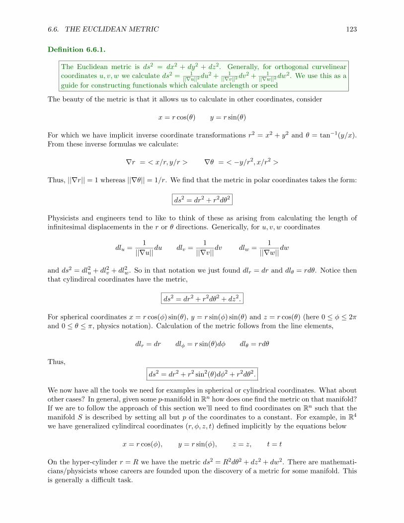
6.6. THE EUCLIDEAN METRIC 123
Definition 6.6.1.
The Euclidean metric is ds2 = dx2 + dy2 + dz2. Generally, for orthogonal curvelinearcoordinates u, v, w we calculate ds2 = 1
||∇u||2du2 + 1
||∇v||2dv2 + 1
||∇w||2dw2. We use this as a
guide for constructing functionals which calculate arclength or speed
The beauty of the metric is that it allows us to calculate in other coordinates, consider
x = r cos(θ) y = r sin(θ)
For which we have implicit inverse coordinate transformations r2 = x2 + y2 and θ = tan−1(y/x).From these inverse formulas we calculate:
∇r = < x/r, y/r > ∇θ = < −y/r2, x/r2 >
Thus, ||∇r|| = 1 whereas ||∇θ|| = 1/r. We find that the metric in polar coordinates takes the form:
ds2 = dr2 + r2dθ2
Physicists and engineers tend to like to think of these as arising from calculating the length ofinfinitesimal displacements in the r or θ directions. Generically, for u, v, w coordinates
dlu =1
||∇u||du dlv =
1
||∇v||dv dlw =
1
||∇w||dw
and ds2 = dl2u + dl2v + dl2w. So in that notation we just found dlr = dr and dlθ = rdθ. Notice thenthat cylindircal coordinates have the metric,
ds2 = dr2 + r2dθ2 + dz2.
For spherical coordinates x = r cos(φ) sin(θ), y = r sin(φ) sin(θ) and z = r cos(θ) (here 0 ≤ φ ≤ 2πand 0 ≤ θ ≤ π, physics notation). Calculation of the metric follows from the line elements,
dlr = dr dlφ = r sin(θ)dφ dlθ = rdθ
Thus,
ds2 = dr2 + r2 sin2(θ)dφ2 + r2dθ2.
We now have all the tools we need for examples in spherical or cylindrical coordinates. What aboutother cases? In general, given some p-manifold in Rn how does one find the metric on that manifold?If we are to follow the approach of this section we’ll need to find coordinates on Rn such that themanifold S is described by setting all but p of the coordinates to a constant. For example, in R4
we have generalized cylindircal coordinates (r, φ, z, t) defined implicitly by the equations below
x = r cos(φ), y = r sin(φ), z = z, t = t
On the hyper-cylinder r = R we have the metric ds2 = R2dθ2 + dz2 + dw2. There are mathemati-cians/physicists whose careers are founded upon the discovery of a metric for some manifold. Thisis generally a difficult task.

124 CHAPTER 6. INTRODUCTION TO VARIATIONAL CALCULUS
6.7 geodesics
A geodesic is a path of smallest distance on some manifold. In general relativity, it turns out thatthe solutions to Eistein’s field equations are geodesics in 4-dimensional curved spacetime. Particlesthat fall freely are following geodesics, for example projectiles or planets in the absense of otherfrictional/non-gravitational forces. We don’t follow a geodesic in our daily life because the earthpushes back up with a normal force. Also, do be honest, the idea of length in general relativity is abit more abstract that the geometric length studied in this section. The metric of general relativityis non-Euclidean. General relativity is based on semi-Riemannian geometry whereas this sectionis all Riemannian geometry. The metric in Riemannian geometry is positive definite. The metricin semi-Riemannian geometry can be written as a quadratic form with both positive and negativeeigenvalues. In any event, if you want to know more I know some books you might like.
6.7.1 geodesic on cylinder
The equation of a cylinder of radius R is most easily framed in cylindrical coordinates (r, θ, z); theequation is merely r = R hence the metric reads
ds2 = R2dθ2 + dz2
Therefore, we ought to minimize the following functional in order to locate the parametric equationsof a geodesic on the cylinder: note ds2 =
(R2 dθ2
dt2+ dz2
dt2
)dt2 thus:
S =
∫(R2θ2 + z2) dt
Euler-Lagrange equations for the dependent variables θ and z are simply:
θ = 0 z = 0.
We can integrate twice to find solutions
θ(t) = θo +At z(t) = zo +Bt
Therefore, the geodesic on a cylinder is simply the line connecting two points in the plane which iscurved to assemble the cylinder. Simple cases that are easy to understand:
1. Geodesic from (R cos(θo), R sin(θo), z1) to (R cos(θo), R sin(θo), z2) is parametrized by θ(t) =θo and z(t) = z1 + t(z2 − z1) for 0 ≤ t ≤ 1. Technically, there is some ambiguity here since Inever declared over what range the t is to range. Could pick other intervals, we could use zat the parameter is we wished then θ(z) = θo and z = z for z1 ≤ z ≤ z2
2. Geodesic from (R cos(θ1), R sin(θ1), zo) to (R cos(θ2), R sin(θ2), zo) is parametrized by θ(t) =θ1 + t(θ2 − θ1) and z(t) = zo for 0 ≤ t ≤ 1.
3. Geodesic from (R cos(θ1), R sin(θ1), z1) to (R cos(θ2), R sin(θ2), z2) is parametrized by
θ(t) = θ1 + t(θ2 − θ1) z(t) = z1 + t(z2 − z1)
You can eliminate t and find the equation z = z2−z1θ2−θ1 (θ − θ1) which again just goes to show
you this is a line in the curved coordinates.

6.8. LAGRANGIAN MECHANICS 125
6.7.2 geodesic on sphere
The equation of a sphere of radius R is most easily framed in spherical coordinates (r, φ, θ); theequation is merely r = R hence the metric reads
ds2 = R2 sin2(θ)dφ2 +R2dθ2.
Therefore, we ought to minimize the following functional in order to locate the parametric equations
of a geodesic on the sphere: note ds2 =(R2 sin2(θ)dφ
2
dt2+R2 dθ2
dt2
)dt2 thus:
S =
∫( R2 sin2(θ)φ2 +R2θ2︸ ︷︷ ︸
f(θ,φ,θ,φ)
) dt
Euler-Lagrange equations for the dependent variables φ and θ are simply: fθ = ddt(fθ) and fφ =
ddt(fφ) which yield:
2R2 sin(θ) cos(θ)φ2 = ddt(2R
2θ) 0 =d
dt
(2R2 sin2(θ)φ
).
We find a constant of motion L = 2R2 sin2(θ)φ inserting this in the equation for the azmuthialangle θ yields:
2R2 sin(θ) cos(θ)φ2 = ddt(2R
2θ) 0 =d
dt
(2R2 sin2(θ)φ
).
If you can solve these and demonstrate through some reasonable argument that the solutions aregreat circles then I will give you points. I have some solutions but nothing looks too pretty.
6.8 Lagrangian mechanics
6.8.1 basic equations of classical mechanics summarized
Classical mechanics is the study of massive particles at relatively low velocities. Let me refreshyour memory about the basics equations of Newtonian mechanics. Our goal in this section will beto rephrase Newtonian mechanics in the variational langauge and then to solve problems with theEuler-Lagrange equations. Newton’s equations tell us how a particle of mass m evolves throughtime according to the net-force impressed on m. In particular,
md2~r
dt2= ~F
If m is not constant then you may recall that it is better to use momentum ~P = m~v = md~rdt to
set-up Newton’s 2nd Law:
d~P
dt= ~F
In terms of components we have a system of differential equations with indpendent variable timet. If we use position as the dependent variable then Newton’s 2nd Law gives three second orderODEs,
mx = Fx my = Fy mz = Fz
where ~r = (x, y, z) and the dots denote time-derivatives. Moreover, ~F =< Fx, Fy, Fz > is the sumof the forces that act on m. In contrast, if you work with momentum then you would want to solvesix first order ODEs,
Px = Fx Py = Fy Pz = Fz

126 CHAPTER 6. INTRODUCTION TO VARIATIONAL CALCULUS
and Px = mx, Py = my and Pz = mz. These equations are easiest to solve when the force is
not a function of velocity or time. In particular, if the force ~F is conservative then there exists apotential energy function U : R3 → R such that ~F = −∇U . We can prove that in the case theforce is conservative the total energy is conserved.
6.8.2 kinetic and potential energy, formulating the Lagrangian
Recall the kinetic energy is T = 12m||~v||
2, in Cartesian coordinates this gives us the formula:
T =1
2m(x2 + y2 + z2).
If ~F is a conservative force then it is independent of path so we may construct the potential energyfunction as follows:
U(~r) = −∫ ~r
O~F · d~r
Here O is the origin for the potential and we can prove that the potential energy constructed inthis manner has ~F = −∇U . We can prove that the total (mechanical) energy E = T + U fora conservative system is a constant; dE/dt = 0. Hopefully these comments are at least vaguelyfamiliar from some physics course in your distant memory. If not relax, calculationally this chapteris self-contained, read onward.
We already calculated that if we use T as the Lagrangian then the Euler-Lagrange equationsproduce Newton’s equations in the case that the force is zero (see 6.5.1). Suppose that we definethe Lagrangian to be L = T−U for a system governed by a conservative force with potential energyfunction U . We seek to prove the Euler-Lagrange equations are precisely Newton’s equations forthis conservative system1 Generically we have a Lagrangian of the form
L(x, y, z, x, y, z) =1
2m(x2 + y2 + z2)− U(x, y, z).
We wish to find extrema for the functional S =∫L(t) dt. This yields three sets of Euler-Lagrange
equations, one for each dependent variable x, y or z
d
dt
[∂L
∂x
]=∂L
∂x
d
dt
[∂L
∂y
]=∂L
∂y
d
dt
[∂L
∂z
]=∂L
∂z.
Note that ∂L∂x = mx, ∂L
∂y = my and ∂L∂z = mz. Also note that ∂L
∂x = −∂U∂x = Fx, ∂L
∂y = −∂U∂y = Fy
and ∂L∂z = −∂U
∂z = Fz. It follows that
mx = Fx my = Fy mz = Fz.
Of course this is precisely m~a = ~F for a net-force ~F =< Fx, Fy, Fz >. We have shown thatHamilton’s principle reproduces Newton’s Second Law for conservative forces. Let me take amoment to state it.
1don’t mistake this example as an admission that Lagrangian mechanics is limited to conservative systems. Quitethe contrary, Lagrangian mechanics is actually more general than the orginal framework of Newton!

6.8. LAGRANGIAN MECHANICS 127
Definition 6.8.1. Hamilton’s Principle:
If a physical system has generalized coordinates qj with velocities qj and Lagrangian L =T − U then the solutions of physics will minimize the action S defined below:
S =
∫ t2
t1
L(qj , qj , t) dt
Mathematically, this means the variation δS = 0 for physical trajectories.
This is a necessary condition for solutions of the equations of physics. Sufficient conditions areknown, you can look in any good variational calculus text. You’ll find analogues to the secondderivative test for variational differentiation. As far as I can tell physicists don’t care about thislogical gap, probably because the solutions to the Euler-Lagrange equations are the ones for whichthey are looking.
6.8.3 easy physics examples
Now, you might just see this whole exercise as some needless multiplication of notation and for-malism. After all, I just told you we just get Newton’s equations back from the Euler-Lagrangeequations. To my taste the impressive thing about Lagrangian mechanics is that you get to startthe problem with energy. Moreover, the Lagrangian formalism handles non-Cartesian coordinateswith ease. If you search your memory from classical mechanics you’ll notice that you either doconstant acceleration, circular motion or motion along a line. What if you had a particle con-strained to move in some frictionless ellipsoidal bowl. Or what if you had a pendulum hanging offanother pendulum? How would you even write Newtons’ equations for such systems? In contrast,the problem is at least easy to set-up in the Lagrangian approach. Of course, solutions may be lesseasy to obtain.
Example 6.8.2. Projectile motion: take z as the vertical direction and suppose a bullet is firedwith initial velocity vo =< vox, voy, voz >. The potential energy due to gravity is simply U = mgzand kinetic energy is given by T = 1
2m(x2 + y2 + z2). Thus,
L =1
2m(x2 + y2 + z2)−mgz
Euler-Lagrange equations are simply:
d
dt
[mx
]= 0
d
dt
[my
]= 0
d
dt
[mz
]=
∂
∂z(−mgz) = −mg.
Integrating twice and applying initial conditions gives us the (possibly familiar) equations
x(t) = xo + voxt, y(t) = yo + voyt, z(t) = zo + vozt− 12gt
2.
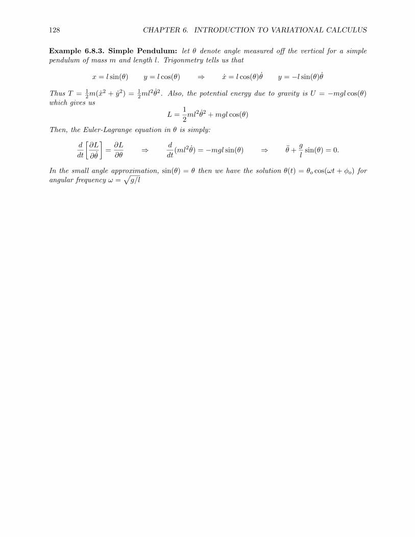
128 CHAPTER 6. INTRODUCTION TO VARIATIONAL CALCULUS
Example 6.8.3. Simple Pendulum: let θ denote angle measured off the vertical for a simplependulum of mass m and length l. Trigonmetry tells us that
x = l sin(θ) y = l cos(θ) ⇒ x = l cos(θ)θ y = −l sin(θ)θ
Thus T = 12m(x2 + y2) = 1
2ml2θ2. Also, the potential energy due to gravity is U = −mgl cos(θ)
which gives us
L =1
2ml2θ2 +mgl cos(θ)
Then, the Euler-Lagrange equation in θ is simply:
d
dt
[∂L
∂θ
]=∂L
∂θ⇒ d
dt(ml2θ) = −mgl sin(θ) ⇒ θ +
g
lsin(θ) = 0.
In the small angle approximation, sin(θ) = θ then we have the solution θ(t) = θo cos(ωt + φo) forangular frequency ω =
√g/l