Embed Size (px)
Citation preview

Calculus: An Integrated Approachby Matt Cathey and Joseph SpiveyWofford College
Created with Mathematica

3The Derivative
Contents:1. The Tangent Line Problem2. Defining the Derivative3. The Derivative Function4. Derivative Formulas5. Higher Derivatives6. Antiderivatives7. Differential Equations and Initial Value Problems
1. The Tangent Line ProblemNow that we know how to evaluate limits, we’re ready to turn our attention to one of the seminal problems of calculus: finding lines that aretangent to graphs of functions. The usage of the word “tangent” here is related to the way we use the word in geometry in relation to circles: Aline is tangent to a circle if it intersects the circle in exactly one point, as in this figure:
2 Ch3.nb

angle
While that definition of “tangent line” works just fine for circles, it does not extend to graphs of arbitrary functions. For example, the graph off (x) = x3 is intersected only once by the line y = x + 1, but the line y = 3 x - 2 looks more like we’d expect a tangent line to look like (eventhough it intersects the graph of f (x) twice):
-3 -2 -1 1 2 3
-10
-5
5
10
x3
x+1
3x-2
So, what exactly do we mean by line tangent to a graph? We’ll give a formal definition soon, but the way we will picture it is by imaginingdriving along a moonlit road in exactly the shape of our graph. The tangent line at the point our car occupies is the line defined by our head-lights. Returning to f (x) = x3, picture the graph as a road. Drag the slider to move the car along the road; the direction of its headlights is givenby the orange line. Now, uncheck the box labeled “Show car?” to show the full tangent line.
Ch3.nb 3

x
Show car?
Now that we have a better idea of what the tangent line is, we need to figure out how to find it. Let’s say we wish to find the line tangent to thegraph of f (x) = x3 at the point where x = 2. Since f (2) = 8, we know one point on the line: (2, 8). Recall from Chapter 1 that we need twopieces of information in order to find the equation of a line: the slope and a point (or two points, from which we can compute the slope). That’sa problem here; the only point we know for sure that this line passes through is the point (2, 8), and we don’t know the slope. So, what do wedo? Take a look at this graph of f (x) = x3, along with its tangent line at (2, 8) and (in keeping with geometric terminology) a secant line (whichintersects the graph twice: at (2, 8) and s, s3):
s 1.475
1.475
3.209
8
-1 1 2 3 4
-5
5
10
15
20
25
30
We can see that the green secant line is very close to the orange tangent line whenever s is close to 2. In fact, the closer s is to 2, the closer thesecant line is to the tangent line. So, what is the slope of the secant line? We know it passes through the points (2, 8) and s, s3, so the slope
must be s3-8s-2
. Notice that, if s = 2, the expression for the slope has a zero in both the denominator and numerator; this happens because we needtwo points to compute a slope, and if s = 2, we only have one point. Move the slider so that s has a value near 2, and compute the slope. Canyou make it get any closer? After a point, this tool can only do so much, but it appears that the slope of the secant line gets closer and closer tothe slope of the tangent line as a approaches 2. So, we will say that the slope of the tangent line is the limit as s approaches 2 of the slope of the
secant line. In other words, if we use the symbol mtangent to denote the slope of the tangent line, mtangent = lims→2
s3-8s-2
. Looking at tables, we get
the following:
4 Ch3.nb

We can see that the green secant line is very close to the orange tangent line whenever s is close to 2. In fact, the closer s is to 2, the closer thesecant line is to the tangent line. So, what is the slope of the secant line? We know it passes through the points (2, 8) and s, s3, so the slope
must be s3-8s-2
. Notice that, if s = 2, the expression for the slope has a zero in both the denominator and numerator; this happens because we needtwo points to compute a slope, and if s = 2, we only have one point. Move the slider so that s has a value near 2, and compute the slope. Canyou make it get any closer? After a point, this tool can only do so much, but it appears that the slope of the secant line gets closer and closer tothe slope of the tangent line as a approaches 2. So, we will say that the slope of the tangent line is the limit as s approaches 2 of the slope of the
secant line. In other words, if we use the symbol mtangent to denote the slope of the tangent line, mtangent = lims→2
s3-8s-2
. Looking at tables, we get
the following:
s s3-8s-2
1 71.9 11.411.99 11.94011.999 11.994001.9999 11.999401.99999 11.99994
s s3-8s-2
3 192.1 12.612.01 12.06012.001 12.006002.0001 12.000602.00001 12.00006
It would seem that the limit is 12; let’s try to verify using algebra. For this computation, we’ll need a factorization formula known as thedifference of cubes formula: a3 - b3 = (a - b) a2 + a b + b2, which can be verified by multiplying out the right side. Thus,
mtangent = lims→2
s3-8s-2
= lims→2
(s-2) s2+2 s+4
s-2(difference of cubes, with a = s and b = 2)
= lims→2
s2 + 2 s + 4 (canceling s - 2)
= 22 + 2 ·2 + 4 (evaluating the limit using continuity)= 12 (simplifying).
Our guess was correct! Since the tangent line has slope 12 and passes through the point (2, 8), we know its equation: y - 8 = 12 (x - 2) in point-slope form, or y = 12 x - 16 in slope-intercept form. Finding slopes of tangent lines is one of the fundamental problems in calculus; we willspend quite a bit of time working toward making that computation as easy as possible. We begin that process in the next section.
2. Defining the DerivativeWe start our exploration of slopes of tangent lines with a definition that is reminiscent of the discussion in the previous section.
Let f (x) be a function defined on the interval (p, q), and let a be a number in that interval. Then the derivative off(x) at x = a is the limit as x approaches a of f (x)- f (a)
x-a, if it exists. Symbolically, we write either f ′(a) = lim
x→a
f (x)- f (a)x-a
orddx
f (x) x=a = limx→a
f (x)- f (a)x-a
.
(Note: There are two ways to denote the derivative in large part because, as we saw in the opening chapter, there were two men who discoveredcalculus: Newton and Leibniz. The notation above on the left, read “ f prime of a,” comes from the notation used by Newton; the notation onthe right, read “d d x of f of x at x = a” or simply “the derivative of f of x at x = a,” is the notation developed by Leibniz. Each has itsadvantages and drawbacks; in what follows, we will use both.)The limit in the definition looks familiar: it’s the limit of the slopes of secant lines. Thus, we will interpret the derivative as follows:
The derivative of f (x) at x = a is the slope of the line tangent to the graph of f (x) at the point (a, f (a)).
Further, if we interpret the slopes as rates of change, we get this:
The slopes of secant lines are average rates of change; the slopes of tangent lines are instantaneous rates of change.
Let’s work through an example. Given f (x) = 3 x3 + 7 x2 - 8 x - 6, let’s compute f ′(1):
f ′(1) = limx→1
f (x)- f (1)x-1
(definition of derivative)
= limx→1
3 x3+7 x2-8 x-6-(-4)
x-1(substituting; be careful with the negative !)
= limx→1
3 x3+7 x2-8 x-2x-1
(simplifying)
= limx→1
(x-1) 3 x2+10 x+2
x-1(factoring the numerator)
= limx→1
3 x2 + 10 x + 2 (canceling x - 1)
= 15 (by continuity).
Ch3.nb 5

f ′(1) = limx→1
f (x)- f (1)x-1
(definition of derivative)
= limx→1
3 x3+7 x2-8 x-6-(-4)
x-1(substituting; be careful with the negative !)
= limx→1
3 x3+7 x2-8 x-2x-1
(simplifying)
= limx→1
(x-1) 3 x2+10 x+2
x-1(factoring the numerator)
= limx→1
3 x2 + 10 x + 2 (canceling x - 1)
= 15 (by continuity).
The computation is fairly straightforward, except the step where we factor the numerator. For complicated functions like the one we justconsidered, that factorization may not be terribly easy. Fortunately, there’s a way around that. We’ll make a substitution: let x - 1 = h. Thenx = 1 + h, and as x approaches 1, h approaches 0. So, we get the following:
f ′(1) = limx→1
f (x)- f (1)x-1
(definition of derivative)
= limh→0
f 1+h- f (1)
h(substituting)
= limh→0
3 1+h3+7 1+h2-8 1+h-6-(-4)
h(plugging in)
= limh→0
3 1+3 h+3 h2+h3+7 1+2 h+h2-8 1+h-6+4
h(expanding binomials)
= limh→0
3+9 h+9 h2+3 h3+7+14 h+7 h2-8-8 h-6+4h
(distributing)
= limh→0
3+7-8-6+4+9 h+14 h-8 h+9 h2+7 h2+3 h3
h(collecting like terms)
= limh→0
0+15 h+16 h2+3 h3
h(simplifying)
= limh→0
h15+16 h+3 h2
h(factoring numerator)
= limh→0
15 + 16 h + 3 h2 (canceling h)
= 15 (by continuity).
That took a few more steps, and we had to expand binomials. But the factoring was much easier; we simply had to factor out the h from thenumerator. In general, expanding binomials tends to be easier than factoring polynomials, but your experience may be different. For those whowish to use the latter method, we present this alternate definition of the derivative:
By making a substitution, we can alternatively define the derivative as f ′(a) = limh→0
f a+h- f (a)
h.
Let’s look at a diagram to help us understand why the two definitions are equivalent. Here again, we’re considering the slope of the linetangent to the graph of f (x) = x3 at x = 2. This time, you can move the slider to make x approach 2; at the same time, look at what happens to h,which is labeled in red; its value is given at the top.
6 Ch3.nb

a 1
x
f (x)
8
h-1 1 2 3 4
-5
5
10
15
20
25
30h = -1.000
In what follows, we will most frequently use this latter definition. Both are equally valid, so either may be used at any time.
Example 1 (Computing derivatives):
Given the following functions, compute the requested derivatives.
1. g(x) = x4 - 4 x2 + 4; g′(3)2. r(t) = 1
t2-1; r′(-2)
3. f (x) = 5 - x ; f ′(1)
Solution.
1. Using the alternate definition, we get:
g′(3) = limh→0
g3+h-g3
h(definition of derivative )
= limh→0
3+h4-4 3+h2+4-49
h(substituting )
= limh→0
81+108 h+54 h2+12 h3+h4-4 9+6 h+h2+4-49
h(expanding binomials )
= limh→0
81+108 h+54 h2+12 h3+h4-36-24 h-4 h2+4-49h
(distributing )
= limh→0
81-36+4-49+108 h-24 h+54 h2-4 h2+12 h3+h4
h(grouping like terms )
= limh→0
0+84 h+50 h2+12 h3+h4
h(simplifying )
= limh→0
h84+50 h+12 h2+h3
h(factoring )
= limh→0
84 + 50 h + 12 h2 + h3 (canceling the h)
= 84 (by continuity ).
2. We’ll again use the alternate definition. For this one, we’ll apply a technique we developed in the last chapter tosimplify the fractions. Since r(t) = 1
t2-1, we get:
r′(-2) = limh→0
r-2+h-r(-2)
h(definition of derivative )
= limh→0
1
(-2+h)2-1-
1
(-2)2-1
h(substitution )
= limh→0
1
3-4 h+h2-
1
3
h·
3 3-4 h+h2
3 3-4 h+h2(simplification, Fancy One )
= limh→0
3-3-4 h+h2
h 3 3-4 h+h2(distributing the numerator, simplifying )
= limh→0
4 h-h2
3 h 3-4 h+h2(simplifying )
= limh→0
h4-h
3 h 3-4 h+h2(factoring numerator )
= limh→0
4-h3 3-4 h+h2
(canceling h)
= 4-03 3-4 (0)+(0)2
(by continuity )
= 49
(simplifying ).
Ch3.nb 7

r′(-2) = limh→0
r-2+h-r(-2)
h(definition of derivative )
= limh→0
1
(-2+h)2-1-
1
(-2)2-1
h(substitution )
= limh→0
1
3-4 h+h2-
1
3
h·
3 3-4 h+h2
3 3-4 h+h2(simplification, Fancy One )
= limh→0
3-3-4 h+h2
h 3 3-4 h+h2(distributing the numerator, simplifying )
= limh→0
4 h-h2
3 h 3-4 h+h2(simplifying )
= limh→0
h4-h
3 h 3-4 h+h2(factoring numerator )
= limh→0
4-h3 3-4 h+h2
(canceling h)
= 4-03 3-4 (0)+(0)2
(by continuity )
= 49
(simplifying ).
3. This time, we’ll need the technique we saw in the last chapter for handling limits involving radicals. Sincef (x) = 5 - x , we have:
f ′(1) = limh→0
f 1+h- f (1)
h(definition of derivative )
= limh→0
5-1+h - 5-1
h(substitution )
= limh→0
4-h -2h
· 4-h +2
4-h +2(simplifying, Fancy One )
= limh→0
4-h-4
h 4-h +2(difference of squares )
= limh→0
-h
h 4-h +2(simplifying )
= limh→0
h (-1)
h 4-h +2(factoring out h)
= limh→0
-1
4-h +2(canceling h)
= -1
4-0 +2(by continuity )
= - 14
(simplifying ).
Example 2 (Finding equations of tangent lines):
Find the equations of the tangent lines in Example 1, and graph both the original function and the tangent line.
Solution.
1. We found that, for g(x) = x4 - 4 x2 + 4, g′(3) = 84. So, the tangent line is the line with slope 84 passing through thepoint (3, g(3)) = (3, 49). Using point-slope form, the line we seek has equation y - 49 = 84 (x - 3); solving for y yieldsy = 84 x - 203. Let’s check the graph to make sure we’ve got the right line:
8 Ch3.nb

-1 1 2 3 4
-20
20
40
60
80
100
x4-4x2+4
84x-203
2. In the second part of the example above, we found that if r(t) = 1t2-1
, then r′(-2) = 49
. The tangent line must pass
through the point (-2, r(-2)) = -2, 13. So, the equation of the tangent line is y - 1
3= 4
9(t - (-2)), which is equivalent
to y = 49
t + 119
. Let’s check the graph:
-3 -2 -1 1
-2
-1
1
2
1t2-1
4 t9 +
119
3. Finally, we saw that if f (x) = 5 - x , then f ′(1) = - 14
. So, the tangent line has slope - 14
and passes through
(1, f (1)) = (1, 2). Thus, the tangent line has equation y - 2 = - 14(x - 1), or y = - 1
4x + 9
4. Here’s the graph:
-1 1 2 3 4 5
0.5
1.0
1.5
2.0
2.5
5 - x
- x4+94
We’ll close our discussion with one more example.
Ch3.nb 9
Example 3 (Derivatives at more than one point):
Given f (x) = 3x-1
, compute the following:
1. f ′(2)2. f ′(3)3. f ′(4)4. f ′(10)5. f ′(15)6. f ′(20)7. f ′(50)8. f ′(100)
Solution.
1. Let’s use the alternate definition again:
f ′(2) = limh→0
f 2+h- f (2)
h(definition of derivative )
= limh→0
3
(2+h)-1-
3
2-1
h(substituting )
= limh→0
3
1+h-3
h· 1+h
1+h(simplifying, Fancy One )
= limh→0
3
1+h1+h-3 1+h
h 1+h(distributing )
= limh→0
3-3-3 hh 1+h
(simplifying )
= limh→0
-3 hh 1+h
(simplifying )
= limh→0
-31+h
(canceling h)
= -31
(by continuity )
= -3 (simplifying ).
2. As before:
f ′(3) = limh→0
f 3+h- f 3
h(definition of derivative )
= limh→0
3
(3+h)-1-
3
3-1
h(substituting )
= limh→0
3
2+h-
3
2
h·
2 2+h
2 2+h(simplifying,Fancy One )
= limh→0
3
2+h(2) 2+h-
3
2(2) 2+h
h (2) 2+h(distributing )
= limh→0
6-6-3 hh (2) 2+h
(simplifying )
= limh→0
-3 hh (2) 2+h
(simplifying )
= limh→0
-32 2+h
(canceling h)
= -32 (2)
(by continuity )
= - 34
(simplifying ).
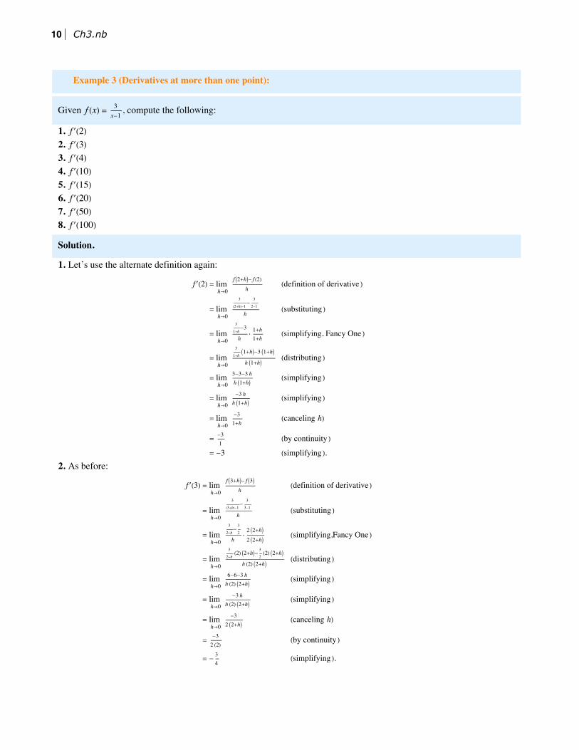
10 Ch3.nb
3. Hey, wait a minute... We followed the exact same steps in the solution of part 2 as in part 1. Perhaps there’s a way toautomate this process; let’s hold off on the rest of this example until the next section.
3. The Derivative FunctionIn Example 3, we were asked to find the value of the derivative of a function at several points; we noticed that, in the first two cases at least, theprocess of actually finding the derivative was the same. Wouldn’t it be easier if we had a formula for the derivative, into which we couldsimply plug in numbers?
Example 3, continued.
Recall that the alternate definition of the derivative says that f ′(a) = limh→0
f (a+h)- f (a)h
. In every example before now,
we’ve plugged in a number for a right at the very beginning; let’s resist that urge, and see how far we can get:
f ′(a) = limh→0
f a+h- f (a)
h(definition of derivative )
= limh→0
3
(a+h)-1-
3
a-1
h(substituting )
= limh→0
3
a+h-1-
3
a-1
h·a+h-1 (a-1)
a+h-1 (a-1)(Fancy One )
= limh→0
3
a+h-1a+h-1 (a-1)-
3
a-1a+h-1 (a-1)
h a+h-1 (a-1)(distributing )
= limh→0
3 (a-1)-3 a+h-1
h a+h-1 (a-1)(simplifying )
= limh→0
3 a-3-3 a-3 h+3h a+h-1 (a-1)
(simplifying )
= limh→0
-3 hh a+h-1 (a-1)
(simplifying )
= limh→0
-3a+h-1 (a-1)
(canceling h)
= -3(a+0-1) (a-1)
(by continuity )
= - 3(a-1)2
(simplifying ).
So, f ′(a) = - 3(a-1)2
; that means f ′(4) = - 3(4-1)2
= - 13
, f ′(10) = - 3(10-1)2
= - 127
, f ′(15) = - 3(15-1)2
= - 3196
,
f ′(20) = - 3(20-1)2
= - 3361
, f ′(50) = - 3(50-1)2
= - 32401
, and f ′(100) = - 3(100-1)2
= - 13267
.
By taking the limit once with a symbol (a) standing in for the number we’re investigating, we were able to find the rest of the derivatives justby plugging those numbers into the formula we got after taking the limit. Of course, there’s nothing special about the symbol a; we could justas easily have used x. That brings us to our next definition.
Let f (x) be a function. Then the derivative of f (x) is the function f ′ (x) = limh→0
f (x+h)- f (x)h
. The domain of this func-
tion is the same as the domain of f , except we remove any numbers for which that limit does not exist.
So, rephrasing the result of Example 3, if f (x) = 3x-1
, then f ′(x) = - 3(x-1)2
.
This notation for the derivative is based on the notation Newton used in Principia Mathematica. Since he was working independently, Leibniz
came up with a different notation; he denoted the derivative of f (x) as ddx
f (x), or simply df
dx. The former is read as “d-d-x of f (x),” or, more
formally, as “the derivative of f (x) with respect to x.” For our purposes, the “with respect to...” part of that phrase always refers to the indepen-dent variable in the function; that matter becomes more important in multivariable calculus. So, we would express the result of Example 3
using Leibniz notation as ddx
3x-1
= - 3(x-1)2
. This is a little more compact than using the prime notation of Newton. If we wish to talk about the
value of the derivative at a particular point in Leibniz notation, we use a vertical bar with a subscript indicating the substitution:
ddx
3x-1
x=3
= - 33-12
= - 34
. Finally, if our function is stated as a relationship between a dependent and independent variable (as in y = 3x-1
), we
will refer to the derivative as dy
dx.
Ch3.nb 11
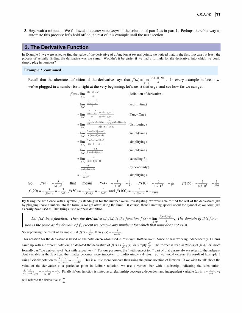
Example 4 (Finding derivatives):
Find the derivatives of the following functions:
1. f (t) = t3 - 2 t2 + 5 t - 42. g(x) = x
x+5
3. r(x) = 3 x + 2
Solution.
1. We’ll apply the definition of the derivative:
f ′(t) = limh→0
f t+h- f (t)
h(definition of derivative )
= limh→0
t+h3-2 t+h2+5 t+h-4-t3-2 t2+5 t-4
h(substituting )
= limh→0
t3+3 t2 h+3 t h2+h3-2 t2+2 t h+h2+5 t+h-4-t3-2 t2+5 t-4
h(expanding binomials )
= limh→0
t3+3 t2 h+3 t h2+h3-2 t2-4 t h-2 h2+5 t+5 h-4-t3+2 t2-5 t+4h
(distributing )
= limh→0
3 t2 h+3 t h2+h3-4 t h-2 h2+5 hh
canceling t3, 2 t2, 5 t, and 4
= limh→0
h 3 t2+3 t h+h2-4 t-2 h+5
h(factoring out h)
= limh→0
3 t2 + 3 t h + h2 - 4 t - 2 h + 5 (canceling h)
= 3 t2 + 3 t (0) + (0)2 - 4 t - 2 (0) + 5 (by continuity )= 3 t2 - 4 t + 5 (simplifying ).
2. Again using the definition:
g′(x) = limh→0
gx+h-g(x)
h(definition of derivative )
= limh→0
x+h
(x+h+5)-
x
x+5
h·x+h+5 x+5
x+h+5 x+5(substituting, Fancy One )
= limh→0
x+h x+5-x x+h+5
h x+h+5 x+5(distributing, simplifying )
= limh→0
x2+5 x+h x+5 h-x2-h x-5 xh x+h+5 x+5
(distributing )
= limh→0
5 hh x+h+5 x+5
canceling x2, 5 x, h x
= limh→0
5x+h+5 x+5
(canceling h)
= 5x+0+5 x+5
(by continuity )
= 5x+52
(simplifying ).
3. Applying the definition one more time:
r′(x) = limh→0
rx+h-r(x)
h(definition of derivative )
= limh→0
3 x+h+2 - 3 x+2
h(substituting )
= limh→0
3 x+3 h+2 - 3 x+2h
· 3 x+3 h+2 + 3 x+2
3 x+3 h+2 + 3 x+2(distributing, Fancy One )
= limh→0
3 x+3 h+2-3 x+2
h 3 x+3 h+2 + 3 x+2(difference of squares )
= limh→0
3 h
h 3 x+3 h+2 + 3 x+2(simplifying )
= limh→0
3
3 x+3 h+2 + 3 x+2(canceling h)
= 3
3 x+3 (0)+2 + 3 x+2(by continuity )
= 3
2 3 x+2(simplifying ).
12 Ch3.nb

r′(x) = limh→0
rx+h-r(x)
h(definition of derivative )
= limh→0
3 x+h+2 - 3 x+2
h(substituting )
= limh→0
3 x+3 h+2 - 3 x+2h
· 3 x+3 h+2 + 3 x+2
3 x+3 h+2 + 3 x+2(distributing, Fancy One )
= limh→0
3 x+3 h+2-3 x+2
h 3 x+3 h+2 + 3 x+2(difference of squares )
= limh→0
3 h
h 3 x+3 h+2 + 3 x+2(simplifying )
= limh→0
3
3 x+3 h+2 + 3 x+2(canceling h)
= 3
3 x+3 (0)+2 + 3 x+2(by continuity )
= 3
2 3 x+2(simplifying ).
Let’s take a quick look at some things that all of these computations have in common. First, after doing some algebra in the numerator, everyterm without an h in it canceled out every time. This is typical; in fact, we can use that as a way to check ourselves at the midpoint of thiscomputation. If you simplify as much as possible and you still have a term without an h in it in the numerator, there’s a good chance thatsomething went wrong. Second, the last few steps always involve canceling out an h in the numerator and denominator. Notice that, thoughwe often did lots of algebra in the numerators of those fractions, we never expanded the denominator. That’s why: we know we’ll always needto cancel out that h. Leave it alone down there! One last admonition: there is so much algebra going on here that it’s very, very easy to losetrack of minus signs. Use parentheses as much as possible to avoid that pitfall!Since we can consider the derivative as a function, we can take a look at its graph. How is the graph of a derivative related to the graph of theoriginal function? Since we interpret the derivative as the slope of a tangent line, we can think of the y-value of the derivative function as theslope of the tangent line at the same x-value on the original function. Take a look at this example:
a
-4 -2 2 4
-5
5
10
15
Here, the blue graph is the graph of the original function f (x), the green graph is the tangent line to f (x) at the point (a, f (a)), and the orangegraph is the graph of f ′(x). Notice that when the green line has a negative slope, the graph of the derivative is below the x-axis; that’s becausewhen the tangent line has negative slope, it means the derivative (which is the slope of the tangent line!) is negative. Also, the steeper the greenline is, the farther from the x-axis the graph of the derivative gets. Places where the slope of the green line is zero correspond to places wherethe derivative graph has an x-intercept.Let’s explore what it means for a function to have a derivative.
The function f (x) is differentiable at x = a if f ′(a) exists and f ′(x) is continuous at x = a. Also, f (x) is differen-tiable on a set if it is differentiable at every point in the set. Finally, we say simply that f (x) is differentiable if it isdifferentiable on its domain.
Ch3.nb 13

The function f (x) is differentiable at x = a if f ′(a) exists and f ′(x) is continuous at x = a. Also, f (x) is differen-tiable on a set if it is differentiable at every point in the set. Finally, we say simply that f (x) is differentiable if it isdifferentiable on its domain.
Just like with continuity, differentiability is sometimes better understood in terms of what it isn’t. Since the derivative is defined as a limit, thecases where a derivative doesn’t exist mirror the cases where a limit doesn’t exist.
Example 5 (Differentiability and nondifferentiability):
Explore the nondifferentiability of these functions at the given points.
1. f (x) = x3+1x+1
at x = -1
2. p(x) =x3+1x+1
if x ≠ -15 if x = -1
at x = -1
3. s(x) =x2 if x < 2-x2 if x ≥ 2
at x = 2
4. g(x) = x - 23 + 1 at x = 25. r(x) = 2 + x2 - 1 at x = 1
Solution.
1. Let’s use the first definition of the derivative for this one: f ′(-1) = limx→-1
f (x)- f (-1)x-(-1)
. But f (-1) doesn’t exist; there’s a
zero in the denominator. Had we tried the other definition of the derivative, we’d run into the same problem. So,what’s going on here? Take a look at the graph:
-4 -2 2 4
2
4
6
Since there’s a hole in the graph at x = -1, the function is discontinuous there. Our intuitive definition of the tangentline doesn’t work here; there’s no point for the tangent line to touch. So, the derivative doesn’t exist.
2. Here we’re looking at nearly the same function as before; this time, though, we’re badly attempting to plug the hole:
14 Ch3.nb

-4 -2 2 4
2
4
6
Let’s explore the derivative (actually, the lack of a derivative) graphically first. Remember, the slope of the tangentline is the limit of slopes of secant lines which pass through the points (a, p(a)) and (a + h, p(a + h)); in the labels onthe figure below, ml is the slope of the secant line on the left side of x = -1 and mr is the slope of the secant line on theright.
Ch3.nb 15

left-side h
right-side h
-4 -2 2 4
2
4
6
left-side h = 0.06457 ml = 27.9118right-side h = 0.13804 mr = -17.3507
It appears that the slopes of the secant lines on the left of x = -1 are approaching ∞, while those on the right areapproaching -∞. Either way, it appears the limit in the definition of the derivative doesn’t exist. Let’s look at it froman algebraic standpoint to make sure our suspicion is correct:
limx→-1-
p(x)-p(-1)x-(-1)
= limx→-1-
x3+1
x+1-5
x+1· x+1
x+1(definition of p(x), Fancy One )
= limx→-1-
x3+1-5 (x+1)(x+1)2
(simplification )
= limx→-1-
x3-5 x-4(x+1)2
(simplification )
= limx→-1-
(x+1) x2-x-4
(x+1)2(factoring )
= limx→-1-
x2-x-4x+1
(canceling x + 1)
= ∞ (numerator → -4; denominator → 0 from left )Similar reasoning justifies the claim about the right-hand limit.
3. This function has a jump discontinuity:
16 Ch3.nb

-2 -1 1 2 3
-10
-8
-6
-4
-2
2
4
So, for the same reasons in the previous part of this example, the secant lines on the left will have slopes approaching-∞. From the right, however:
limx→2+
s(x)-s(2)x-2
= limx→2+
-x2-(-4)x-2
(definition of s(x))
= limx→2+
-1 x2-4
x-2(factoring out -1 )
= limx→2+
-1 (x-2) (x+2)x-2
(factoring )
= limx→2+
- 1 (x + 2) (canceling x - 2)
= -1 (2 + 2) (by continuity )= -4 (simplifying ).
Here, the right-hand limit exists! Since the left- and right-hand limits disagree, though, the limit overall fails to exist.Thus, this function has no derivative at x = 2.
4. Take a look at this graph:
Ch3.nb 17

-1 1 2 3 4 5
-1
1
2
3
This function appears to be (and is) continuous at x = 2. So, we won’t run into the same issues as the previous fewparts. Let’s look at some secant lines and their slopes, as before:
18 Ch3.nb

left-side h
right-side h
1 2 3 4
-1
0
1
2
3
left-side h = 0.43152 ml = 1.7512right-side h = 0.16982 mr = 3.2609
Both limits (from the right and from the left) appear to be infinite. Applying our algebraic techniques, we get:
limx→2
g(x)-g(2)x-2
= limx→2
x-23 +1-1x-2
(definition of g(x))
= limx→2
x-23
x-23 (x-2)23(simplifying numerator, rewriting denominator )
= limx→2
1
(x-2)23canceling x - 23
Notice that the denominator approaches 0 (and is always positive), while the numerator is 1. Thus, we’ll get an infinitelimit. Since the limit of the difference quotients doesn’t exist, the derivative doesn’t exist. From a graphicalstandpoint, this happened because the tangent line is vertical; since the slope computation would involve dividing byzero (try it!), vertical lines have no slope.
5. Let’s take a look at the graph of r(x):
Ch3.nb 19

-3 -2 -1 1 2 3
-1
1
2
3
4
5
This function is continuous at x = 1, but there’s a sharp change of direction on the function there (there’s another atx = -1). Let’s look at the slopes of secant lines in that neighborhood:
left-side h
right-side h
-1 1 2 3
2
3
4
5
6
left-side h = 3.16228 ml = -1.16228right-side h = 2.88403 mr = -4.88403
In this case, the secant lines on the left seem to approach a slope of -2, while those on the right approach a slope of 2.Let’s investigate using algebra; since the left side and the right side seem to disagree, we’ll take the left-hand and right-hand limits separately. Here’s the left-hand limit (notice that, since x is approaching 1 from the left, x is slightly lessthan 1; that means x2 - 1 is negative):
limx→1-
r(x)-r(1)x-1
= limx→1-
2+x2-1-2
x-1(definition of r(x))
= limx→1-
x2-1
x-1(simplifying )
= limx→1-
-1 x2-1
x-1(definition of absolute value )
= limx→1-
-1 (x-1) (x+1)x-1
(factoring )
= limx→1-
- 1 (x + 1) (canceling x - 1)
= -2 (by continuity ).
20 Ch3.nb

Here’s the right-hand limit:
limx→1+
r(x)-r(1)x-1
= limx→1+
2+x2-1-2
x-1(definition of r(x))
= limx→1+
x2-1
x-1(simplifying )
= limx→1+
x2-1x-1
(definition of absolute value )
= limx→1+
(x-1) (x+1)x-1
(factoring )
= limx→1+
x + 1 (canceling x - 1)
= 2 (by continuity ).Since the left- and right-hand limits disagree, the limit (and thus the derivative at x = 1) doesn’t exist.
The justification for parts 1–3 of Example 5, while not constituting a full proof, give us an idea why the following theorem must be true.
Theorem 1 (Differentiability Implies Continuity). If f (x) is not continuous at x = a, then f ′(a) doesn’t exist. Inother words, if f ′ (a) exists, then f (x) is continuous at x = a.
This theorem is very important from a theoretical standpoint; we’ll see it again later in the book.
Parts 4 and 5 of Example 5 show us the two primary ways a continuous function can fail to be differentiable: the tangent line at a point isvertical (as in part 4), or the secant lines on the left approach a different “tangent” than those on the right. This is a direct result of the observa-tion we made that the function had a sharp change of direction at that point; we call such points cusps. Thus, for our purposes, a continuousfunction is differentiable if it has no vertical tangent lines or cusps.
4. Derivative formulasThe process of computing derivatives from the definition can be tedious; in this section, we will develop some formulas we can use to helpmake the process easier. The first few we look at are direct results of the limit laws we studied in the last chapter.First, we will look at constant multiples of a function. Recall that, if c is any constant and lim
x→af (x) exists, then lim
x→ac · f (x) = c · lim
x→af (x). Let
g(x) = c · f (x). Then, if f (x) differentiable,
g′(x) = limh→0
gx+h-g(x)
h(definition of derivative )
= limh→0
c· f x+h-c· f (x)
h(definition of g(x))
= limh→0
c f x+h- f (x)
h(factoring out c)
= limh→0
c ·f x+h- f (x)
h (arithmetic rule )
= c · limh→0
f x+h- f (x)
h(Constant Multiple Limit Law )
= c · f ′(x) (definition of derivative ).
We have just proven the following theorem:
Theorem 2 (Derivatives of Constant Multiples). If f (x) is differentiable and c is any constant, then the derivativeof c · f (x) is c · f ′ (x). In Leibniz notation, d
dx(c · f (x)) = c · d
dxf (x).
Let’s prove another theorem. Suppose s(x) = f (x) + g(x), where f (x) and g(x) are differentiable. The corresponding limit law is the one thatstates lim
x→a( f (x) + g(x)) = lim
x→af (x) + lim
x→ag(x). Let’s look at the derivative of s(x):
s′(x) = limh→0
sx+h-s(x)
h(definition of derivative )
= limh→0
f x+h+gx+h- f (x)+g(x)
h(definition of s(x))
= limh→0
f x+h+gx+h- f (x)-g(x)
h(distributing the minus )
= limh→0
f x+h- f (x)+gx+h-g(x)
h(commutativity )
= limh→0
f x+h- f (x)+gx+h-g(x)
h(associativity )
= limh→0
f x+h- f (x)
h+
gx+h-g(x)
h (arithmetic rule )
= limh→0
f x+h- f (x)
h+ lim
h→0
gx+h-g(x)
h(Sum Limit Law )
= f ′(x) + g′(x) (definition of derivative ).
Ch3.nb 21
s′(x) = limh→0
sx+h-s(x)
h(definition of derivative )
= limh→0
f x+h+gx+h- f (x)+g(x)
h(definition of s(x))
= limh→0
f x+h+gx+h- f (x)-g(x)
h(distributing the minus )
= limh→0
f x+h- f (x)+gx+h-g(x)
h(commutativity )
= limh→0
f x+h- f (x)+gx+h-g(x)
h(associativity )
= limh→0
f x+h- f (x)
h+
gx+h-g(x)
h (arithmetic rule )
= limh→0
f x+h- f (x)
h+ lim
h→0
gx+h-g(x)
h(Sum Limit Law )
= f ′(x) + g′(x) (definition of derivative ).
Using exactly the same steps on the function d(x) = f (x) - g(x), we get that d′(x) = f ′(x) - g′(x). This proves the next theorem:
Theorem 3 (Derivatives of Sums and Differences). If f (x) and g(x) are differentiable, thenddx
( f (x) ±g(x)) = ddx
f (x) ± ddx
g(x).
(Notice that we used Leibniz notation in the statement of that theorem; it was easier than using prime notation because we didn’t have to definethe sum and difference functions (s(x) and d(x)). As we go on, we will typically use whichever notation is simpler.)We are really getting somewhere now! Let’s prove a couple more theorems about specific functions.
Theorem 4 (Derivatives of Constants). Let c be any constant. Then ddx
(c) = 0.
Proof. Let c be a constant, and let f (x) = c. Then, no matter what we plug in for x, f (x) = c. In particular,f (x + h) = c. Then:
f ′(x) = limh→0
f x+h- f (x)
h(definition of derivative )
= limh→0
c-ch
(substituting )
= limh→0
0h
(simplifying )
= limh→0
0 (since h ≠ 0)
= 0 (Constant Limit Law ).
■
The function ι(x) = x is called the identity function for reasons that appear in higher-level math courses (the funny-looking “i” without a dot onit is the lower-case Greek letter iota). We’ll look at its derivative next.
Theorem 5 (Derivative of the Identity). Let ι(x) = x. Then ι′(x) = 1.
Proof. We apply the definition:
ι′(x) = limh→0
ιx+h-ι(x)
h(definition of derivative )
= limh→0
x+h-xh
(definition of ι(x))
= limh→0
hh
(simplification )
= limh→0
1 (since h ≠ 0)
= 1 (Constant Limit Law ).
■
22 Ch3.nb

To this point in this section, we’ve been presenting a bunch of theorems with little sense of their purpose. The proof of this next theorem showshow powerful these little statements can be.
Theorem 6 (Derivatives of Linear Functions). The derivative of a linear function is its slope.
For the sake of comparison, let’s start by looking at a proof relying only on the definition of derivative and the limit laws:
First Proof of Theorem 6. Let f (x) = m x + b, where m and b are constants. Then:
f ′(x) = limh→0
f x+h- f (x)
h(definition of derivative )
= limh→0
m x+h+b-m x+b
h(definition of f (x))
= limh→0
m x+m h+b-m x-bh
(distributing )
= limh→0
m hh
(simplifying )
= limh→0
m (canceling h)
= m (Constant Limit Law ).
■
In contrast, let’s look at an alternate proof, which uses no limits at all:
Second Proof of Theorem 6. Let y = m x + b. Then:dy
dx= d
dx(m x + b) (definition of y)
= ddx
m x + ddx
b (Theorem 3)
= m ddx
x + 0 (Theorems 2 and 4)
= m (1) + 0 (Theorem 5)= m (simplifying ).
■
That second proof demonstrates our goal: to be able to compute derivatives without using limits. Let’s look at an example:
Example 6 (Derivatives of linear functions):
Compute the derivatives of the following functions:
1. y = -3 x + 7
2. y = x-34
3. y = π x + 9
Solution.
1. The slope is -3, so by Theorem 6 we get dydx
= -3.
2. We can rewrite this equation as y = 14
x - 34
, so the slope is 14
. Thus, dydx
= 14
.
3. The slope is π, so dydx
= π.
For much of the next chapter, we will work to develop more of these shortcuts so that we can, as much as possible, avoid resorting to usinglimits to find derivatives. For now, though, we’ll look at one more such rule, which applies to power functions.
Theorem 7 (Power Rule). If n is any constant, then ddx
xn = nxn-1.
We don’t yet have the tools to fully prove this statement; for now, we’ll have to settle for the case where n is a positive integer. For this proof,we’ll use the Binomial Theorem from Chapter 1: for any a and b, and for any positive integer n,
(a + b)n =n0 an b0 +
n1 an-1 b1 +
n2 an-2 b2 + ⋯ +
nn - 1 a1 bn-1 +
nn a0 bn. Two important facts about these binomial coefficients:
no matter what n is, n0 = 1 and
n1 = n.
Ch3.nb 23

We don’t yet have the tools to fully prove this statement; for now, we’ll have to settle for the case where n is a positive integer. For this proof,we’ll use the Binomial Theorem from Chapter 1: for any a and b, and for any positive integer n,
(a + b)n =n0 an b0 +
n1 an-1 b1 +
n2 an-2 b2 + ⋯ +
nn - 1 a1 bn-1 +
nn a0 bn. Two important facts about these binomial coefficients:
no matter what n is, n0 = 1 and
n1 = n.
(Partial) Proof of Theorem 7. Let n be a positive integer, and let f (x) = xn. Then:
f ′(x) = limh→0
f x+h- f (x)
h(definition of derivative )
= limh→0
x+hn-xn
h(definition of f (x))
= limh→0
n0 xn h0+
n1 xn-1 h1+
n2 xn-2 h2+⋯+
nn-1 x hn-1+
nn x0 hn -xn
h(Binomial Theorem )
= limh→0
1 xn+n xn-1 h+n2 xn-2 h2+⋯+
nn-1 x hn-1+
nn hn -xn
h(simplifying )
= limh→0
n xn-1 h+n2 xn-2 h2+⋯+
nn-1 x hn-1+
nn hn
h(canceling xn)
= limh→0
h n xn-1+n2 xn-2 h1+⋯+
nn-1 x hn-2+
nn hn-1
h(factoring out h)
= limh→0
n xn-1 +n2 xn-2 h1 + ⋯ +
nn - 1 x hn-2 +
nn hn-1 (canceling h)
= n xn-1 +n2 xn-2(0) + ⋯ +
nn - 1 x (0) +
nn (0) (by continuity )
= n xn-1 (simplifying ).
■
We’ll address the case where n is not a positive integer after we’ve developed a few more tools; for now, though, we may use the Power Rule tocompute derivatives for any possible n.
Example 7 (Using the Power Rule):
Find the derivatives of the following functions:
1. f (x) = 3 x3 - 6 x2 + 4 x - 12. g(x) = 4
x- 3
x2 + 7x3
3. r(x) = x2-5 x+2
x4
Solution.
1. We’ll use the tricks we’ve developed in this section:
f ′(x) = ddx
3 x3 - 6 x2 + 4 x - 1
= ddx
3 x3 - ddx
6 x2 + ddx
(4 x - 1) (by Theorem 3)
= 3 ddx
x3 - 6 ddx
x2 + 4 (by Theorems 2 and 6)
= 3 3 x2 - 6 (2 x) + 4 (Power Rule )
= 9 x2 - 12 x + 4 (simplifying ).
2. To tackle this one, we’ll need to rewrite using our arithmetic rules:
g′(x) = ddx
4x- 3
x2 + 7x3
= ddx
4 x-1 - 3 x-2 + 7 x-3 (arithmetic rules )
= ddx
4 x-1 - ddx
3 x-2 + ddx
7 x-3 (by Theorem 3)
= 4 ddx
x-1 - 3 ddx
x-2 + 7 ddx
x-3 (by Theorem 2)
= 4 -x-2 - 3 -2 x-3 + 7 -3 x-4 (Power Rule )
= - 4x2 + 6
x3 - 21x4 (simplifying ).
24 Ch3.nb

g′(x) = ddx
4x- 3
x2 + 7x3
= ddx
4 x-1 - 3 x-2 + 7 x-3 (arithmetic rules )
= ddx
4 x-1 - ddx
3 x-2 + ddx
7 x-3 (by Theorem 3)
= 4 ddx
x-1 - 3 ddx
x-2 + 7 ddx
x-3 (by Theorem 2)
= 4 -x-2 - 3 -2 x-3 + 7 -3 x-4 (Power Rule )
= - 4x2 + 6
x3 - 21x4 (simplifying ).
3. Again, we’ll need some arithmetic rules:
r′(x) = ddx
x2-5 x+2
x4
= ddx
x2 - 5 x + 2 x-1/4 (arithmetic rules )
= ddx
x7/4 - 5 x34 + 2 x-1/4 (distributing )
= ddx
x7/4 - ddx
5 x34 + ddx
2 x-1/4 (by Theorem 3)
= ddx
x7/4 - 5 ddx
x34 + 2 ddx
x-1/4 (by Theorem 2)
= 74
x34 - 5 34
x-1/4 + 2 - 14
x-54 (Power Rule )
= 74
x34 - 154
x-1/4 - 12
x-54 (simplifying )
= 7 x2 - 15 x - 2 14
x-54 factoring out 14
x-54
= 7 x2-15 x-2
4 x54(arithmetic rules ).
Parts 2 and 3 of Example 7 highlight a couple of difficulties that often arise when working with the power rule. In part 2, we see how negativeexponents seem to get bigger when subtracting one, and in part 3 we see how we needed to rewrite the function in order to apply the rule in thefirst place. Keep these in mind going forward.
5. Higher DerivativesAs we move forward, it will often be useful for us to consider the derivative of a derivative function. If f (x) is a differentiable function, the
second derivative of f (x) is the function f ′′(x) = ddx
f ′(x). In Leibniz notation, the second derivative of y with respect to x is ddx
dy
dx =
d2 y
dx2 . If
we continue taking derivatives of the resulting derivatives, we get the following notations: degree of derivative Prime notation Leibniz notation
0 f (x) y
1 f ′(x) dy
dx
2 f ′′(x) d2 y
dx2
3 f ′′′(x) d3 y
dx
4 f (4)(x) d4 y
dx4
⋮ ⋮ ⋮
n f (n)(x) dn y
dxn
Notice that, starting with the fourth derivative, we stop adding additional primes and simply indicate the number of derivatives taken inparentheses.
Let’s look at an application. Consider the function s(t) = t3 - 6 t2 + 9 t, which describes the position (in meters) of a particle moving on anumber line over the interval [0, 4] (where t is measured in seconds) as in this figure:
Ch3.nb 25

Out[34]=
t 1.755
We can see the particle starts off moving to the right, then turns around and heads to the left, then heads back to the right. Use the slider to tryto estimate the times when the particle changes direction, and keep those numbers in mind. What does the derivative of s(t) tell us about thissituation? Remember, the derivative of s(t) represents the instantaneous rate of change of s(t) with respect to t. Further, sinces′(a) = limt→a
s(t)-s(a)t-a
, we can infer that the units for s′(a) have the same units as the difference quotient; the numerator is measured in meters and
the denominator in seconds, so s′(t) must have units metersseconds
, or meters per second. If this seems familiar, we looked at a very similar problem atthe beginning and end of Chapter 2, where we investigated the meaning of the instantaneous rate of change of the position of a car. Thus, thederivative of s(t) can be interpreted as the instantaneous velocity v(t) of the particle. Using the results from the previous section,
v(t) = s′(t)
= ddtt3 - 6 t2 + 9 t (definition of s(t))
= ddt
t3 - 6 ddt
t2 + 9 ddt
t (Theorems 3 and 2)
= 3 t2 - 6 (2 t) + 9 (1) (Power Rule )= 3 t2 - 12 t + 9 (simplifying ).
Let’s take a look at the particle and its velocity at the same time. We’ll represent the velocity with an arrow (this choice isn’t arbitrary; velocityis a vector, which has both direction and magnitude. Vectors are frequently depicted as arrows):
t 3.415
If you click on the “+“ next to the slider, you can access animation controls. Push the play button (between the “–” and “+“ buttons), and seewhat happens as t increases. Notice that the particle moves to the left whenever the arrow points left (i.e., when v(t) < 0) and it moves rightwhen the arrow points right. Moreover, the longer the arrow, the faster the particle moves. We also might notice that the particle changesdirection when the velocity is zero (this statement isn’t, in general, true; the particle might slow down and stop without completing a directionchange). When does that occur? Since we have a formula for velocity, we can set it equal to zero and solve:
3 t2 - 12 t + 9 = 03 t2 - 4 t + 3 = 0 (factoring out 3 )3 (t - 1) (t - 3) = 0 (factoring polynomial )
t - 1 = 0 or t - 3 = 0 (product equals 0 means a factor is zero )t = 1 or t = 3 (solving ).
Are those numbers close to your earlier guess?
Now, what about the derivative of v(t) (which is the second derivative of s(t))? It represents the instantaneous rate of change of velocity; bydefinition, v′(t) = limt→a
v(t)-v(a)t-a
, where the numerator has units meters per second and the denominator has units seconds. Thus, v′(t) has units
meters
second
second, which can be simplified using a Fancy One:
meters
second
second× seconds
seconds= meters
seconds2. These units are typically written as “msec2,” read “meters per
second squared.” This rate of change of velocity is called acceleration. Let’s compute the acceleration a(t), using the same techniques we usedto find v(t):
26 Ch3.nb

Now, what about the derivative of v(t) (which is the second derivative of s(t))? It represents the instantaneous rate of change of velocity; bydefinition, v′(t) = limt→a
v(t)-v(a)t-a
, where the numerator has units meters per second and the denominator has units seconds. Thus, v′(t) has units
meters
second
second, which can be simplified using a Fancy One:
meters
second
second× seconds
seconds= meters
seconds2. These units are typically written as “msec2,” read “meters per
second squared.” This rate of change of velocity is called acceleration. Let’s compute the acceleration a(t), using the same techniques we usedto find v(t):
a(t) = v′(t)
= ddt3 t2 - 12 t + 9 (definition of v(t))
= 3 ddt
t2 - 12 ddt
t + ddt
9 (Theorems 3 and 2)
= 3 (2 t) - 12 (1) + 0 (Power Rule, Theorem 4)= 6 t - 12 (simplifying ).
Here, we’ll plot position (blue dot), velocity (orange arrow), and acceleration (green arrow) simultaneously. Animate the figure, and makesome guesses about the relationships among the three quantities:
t 0.645
We can see that the direction of the green (acceleration) arrow indicates the direction that the tip of the orange arrow is moving, just like thedirection of the orange (velocity) arrow indicates the direction that the particle is moving. Looking more closely, we can see that the particle isspeeding up (remember, speed is the absolute value of velocity; it removes the “direction” from the vector) whenever both arrows point in thesame direction; it’s slowing down if the arrows point in opposite directions.
6. AntiderivativesNext, consider the formula s(t) = -16.1 t2 + 9 t + 60, which models the height (in feet) of an object thrown upwards at a velocity of 9 feet persecond from an initial height of 60 feet, where t is measured in seconds. As we have just seen, velocity and acceleration can be found bycomputing the first and second derivatives of the position function, respectively. Thus, in this case, v(t) = -16.1 (2 t) + 9 = -32.2 t + 9 anda(t) = -32.2. Notice that, as described above, v(0) = 9. Also, we know from physics that the acceleration due to gravity near Earth’s surface isconstant: -32.2 feetsecond2. So, everything about our equation checks out.
What if we took the same object and threw it upwards at a velocity of 9 feet /second from an initial height of 60 feet... on Mars? Because Marsis less massive, the acceleration due to gravity on that planet’s surface is smaller: about -12.2 feetsecond2. How can we find an equation thatmodels this situation? Here’s what we know: a(t) = -12.2, v(0) = 9, and s(0) = 60. Let’s focus on that first piece of information. We know theacceleration, and we know that acceleration is the derivative of velocity. So, v′(t) = -12.2. Theorem 6 tells us that the derivative of a linearfunction is the slope; it might be reasonable to assume, then, that v(t) is linear (notice that, in the Earth example, v(t) was linear). In that case,v(t) = -12.2 t + b, where, if we were looking at a graph, b is the y-intercept. If we substitute t = 0, we get v(0) = -12.2 (0) + b = b. But, wealready knew v(0) = 9. Thus, b = 9, so v(t) = -12.2 t + 9 (compare this result to the Earth case). We have a formula for velocity! Since weknow that velocity is the derivative of position, we’re one step closer to finding that formula we need. Looking again at the Earth case above,we see that, when we differentiated the position function, we got -16.1 (2 t) + 9. Perhaps we should write our velocity function in a similarway: v(t) = -12.2 t + 9 = -6.1 (2 t) + 9. So, what function could we differentiate to get this? Well, the derivative of t2 is 2 t, so the derivative of-6.1 t2 is -6.1 (2 t). Also, as before, since 9 is constant, it’s the derivative of a linear function with slope 9. So, it’s reasonable to think thats(t) = -6.1 t2 + 9 t + c (notice that we’re using c instead of b to denote the y-intercept; that’s because we’ve already used b in this computation).Since s(0) = 60 by our assumption, and s(0) = -6.1 (0)2 + 9 (0) + c = c by substitution, we get c = 60. Thus, s(t) = -6.1 t2 + 9 t + 60 seems to fitour criteria!In our discussion of tossing objects on Mars, we went from information about the derivatives of the function in question to a formula for thefunction itself. This process is called antidifferentiation.
Let f (x) be a function, and suppose g(x) = f ′(x). Then f (x) is an antiderivative of g(x).
We tend to use only one notation for antiderivatives: if f (x) is an antiderivative of g(x), we write f (x) = ∫ g(x) dx. The symbol at the front thereis a stretched-out “S”; the reason for this choice will be discussed later. The “dx” on the end is the same “dx” that appears in the bottom of theLeibniz notation for the derivative. (Just like how the Leibniz notation looks like a fraction but actually isn’t, the dx in this notation looks likemultiplication, but isn’t. For now, consider the ∫ and the dx to be a matched set, like opening and closing parentheses.) We read “∫ g(x) dx” as“the integral of g of x, d x.” We use the word “integral” here because antidifferentiation is sometimes called integration; along those samelines, g(x) is called the integrand.
Ch3.nb 27

We tend to use only one notation for antiderivatives: if f (x) is an antiderivative of g(x), we write f (x) = ∫ g(x) dx. The symbol at the front thereis a stretched-out “S”; the reason for this choice will be discussed later. The “dx” on the end is the same “dx” that appears in the bottom of theLeibniz notation for the derivative. (Just like how the Leibniz notation looks like a fraction but actually isn’t, the dx in this notation looks likemultiplication, but isn’t. For now, consider the ∫ and the dx to be a matched set, like opening and closing parentheses.) We read “∫ g(x) dx” as“the integral of g of x, d x.” We use the word “integral” here because antidifferentiation is sometimes called integration; along those samelines, g(x) is called the integrand.There is a small but critical detail hiding in that definition: the use of the indefinite article “an.” Differentiable functions have just one deriva-tive, but if a function has an antiderivative, it always has more than one antiderivative (much more than one, in fact). Let’s investigate.Earlier in this section, we called on Theorem 6, which says that the derivative of a linear function is its slope (which is constant). So, theantiderivative of a constant is a linear function, with that constant as its slope! But, notice that we can’t draw any conclusions at all about the y-intercept of that linear function. It could be any real number! Making this more concrete, let’s say we wanted to compute ∫ 3 dx. We’relooking for a linear function with slope 3... How about f (x) = 3 x? If we compute f ′(x), sure enough we get 3. So, 3 x is an antiderivative of 3.How about g(x) = 3 x + 1? Then g′(x) = 3 + 0 = 3, so 3 x + 1 is also an antiderivative of 3. How about h(x) = 3 x - 18 749 261? We quickly seethat h′(x) = 3 + 0 = 3, so it too is an antiderivative of 3. We’re starting to see that ∫ 3 dx = 3 x ± (any number we want)!
Theorem 8 (Families of Antiderivatives). Suppose f (x) is an antiderivative of g(x). Then, for any constant C,f (x) + C is also an antiderivative of g(x).
Proof. Suppose f (x) is an antiderivative of g(x). That means f ′(x) = g(x), by the definition of antiderivative. Wecompute the derivative of f (x) + C:
ddx
( f (x) + C) = ddx
f (x) + ddx
C (by Theorem 3)
= f ′(x) + 0 (by Theorem 4)= f ′(x) (simplifying )= g(x) (by supposition ).
Thus, f (x) + C is an antiderivative of g(x).
■
When we wish to talk about the most general form of an antiderivative, we will always tack on that “+C” to the end, in order to indicate that wecould be working with any function of that form.In some ways, antidifferentiation acts like differentiation (but certainly not in all ways, as we’ll see in the next chapter). For example, Theorem
3 tells us that ddx
( f (x) + g(x)) = ddx
f (x) + ddx
g(x) = f ′(x) + g′(x). Suppose F(x) and G(x) are antiderivatives of f (x) and g(x), respectively.Then
ddx
(F(x) + G(x)) = ddx
F(x) + ddx
G(x)
= F′(x) + G′(x)= f (x) + g(x).
So, F(x) + G(x) is an antiderivative of f (x) + g(x)! We have just proven the first part of the next theorem, which draws more parallels betweenderivatives and antiderivatives. The proofs of the other parts follow in much the same way.
Theorem 9 (Arithmetic Properties of Integrals). Suppose f (x) and g(x) are functions, and c is any real number.T h e n :
1. (Sum Rule) ∫ f (x) +g(x) dx = ∫ f (x) dx + ∫ g(x) dx2. (Difference Rule) ∫ f (x) - g(x) dx = ∫ f (x) dx - ∫ g(x) dx3. (Constant Multiple Rule) ∫ c · f (x) dx = c · ∫ f (x) dx4. (Identity Rule) ∫ 1 dx = x + C
From this point on, with one exception, every differentiation rule we derive will come with a matching antidifferentiation rule. In fact, we needto go back and pick up one we’ve already missed: the Power Rule.
Theorem 7, continued (Power Rule). If n ≠ -1, then an antiderivative of xn is xn+1
n+1.
Proof. By our earlier theorems, ddx
xn+1
n+1= d
dx 1
n+1xn+1 (arithmetic rules )
= 1n+1
ddx
xn+1 (Theorem 2)
= 1n+1
(n + 1) x(n+1)-1 (Power Rule )
= xn (simplifying ).
28 Ch3.nb

Therefore, an antiderivative of xn is xn+1
n+1.
■
Example 8 (Computing antiderivatives):
Compute the following:
1. ∫ 3 x2 - 4 x + 1 dx
2. ∫ x + 1x2 dx
3. x2-4 x+1
x3dx
Solution.
1. We’ll apply the last three theorems:
∫ 3 x2 - 4 x + 1 dx = ∫ 3 x2 dx - ∫ 4 x dx + ∫ 1 dx (Sum and Difference Rules )
= 3 ∫ x2 dx - 4 ∫ x dx + ∫ 1 dx (Constant Multiple Rule )
= 3 x3
3 - 4 x2
2 + x + C (Identity Rule,Power Rule , and Theorem 8)
= x3 - 2 x2 + x + C (simplifying ).
2. For this one, we need to rewrite first:
∫ x + 1x2 dx = ∫ x1/2 + x-2 dx (arithmetic rules )
= ∫ x1/2 dx + ∫ x-2 dx (Sum Rule )
= x3/2
32+ x-1
-1+ C (Power Rule, Theorem 8)
= 23
x3 - 1x+ C (simplifying ).
Notice that the negative exponent gets smaller (in absolute value) after integrating; it’s very easy to get that mixed up.3. This one also requires a little algebra first:
x2-4 x+1
x3dx = ∫ x2 - 4 x + 1 x-13 dx (arithmetic rules )
= ∫ x53 - 4 x23 + x-13 dx (distributing )
= ∫ x53 dx - 4 ∫ x23 dx + ∫ x-13 dx (Sum, Difference, and Constant Multiple Rules)
= x8/3
83- 4 x5/3
53 + x2/3
23+ C (Theorems 7 and 8)
= 38
x83 - 125
x53 + 32
x23 + C (simplifying ).
7. Differential Equations and Initial Value ProblemsIn the last section, we considered a situation in which the acceleration of gravity on Mars (s′′(t)) was known, along with an initial position (s(0))and velocity (s′(0)) of an object. From that, we could deduce the formula for s(t). This is an example of an initial value problem.
A differential equation is an equation containing a derivative. The order of a differential equation is the maximumof the degrees of derivatives in the equation. A solution of a differential equation is a function which makes thedifferential equation true. An initial value problem is a differential equation together with a collection of initialconditions: particular values of a solution or one of its derivatives.
For example, x2 d2 y
dx2 - x dy
dx+ y = x2 - 1 is a differential equation, because it’s an equation which contains a derivative. It’s a second degree
differential equation, because it has a first derivative and a second derivative; 2 is the maximum degree. The function f (x) = x2 + 4 x - 1 is asolution, because f ′(x) = 2 x + 4, f ′′(x) = 2, and:
x2 f ′′(x) - x f ′(x) + f (x) = x2(2) - x (2 x + 4) + x2 + 4 x - 1 (plugging in f (x))
= 2 x2 - 2 x2 - 4 x + x2 + 4 x - 1 (distributing )= x2 - 1 canceling 2 x2, 4 x.
Ch3.nb 29

x2 f ′′(x) - x f ′(x) + f (x) = x2(2) - x (2 x + 4) + x2 + 4 x - 1 (plugging in f (x))
= 2 x2 - 2 x2 - 4 x + x2 + 4 x - 1 (distributing )= x2 - 1 canceling 2 x2, 4 x.
Notice that g(x) = x2 - 7 x - 1 is also a solution (check it!); there are infinitely many others. To make this an initial value problem, we add two
initial conditions: x2 d2 y
dx2 - x dy
dx+ y = x2 - 1, y(0) = -1, y′(0) = 3 (most commonly, the number of initial conditions given equals the degree
of the differential equation; the reason for this is technical, but it has to do with ensuring the solution is unique). The functionr(x) = x2 + 3 x - 1 is a solution of that initial value problem, since r(0) = -1, r′(x) = 2 x + 3 (and so r′(0) = 3), r′′(x) = 2, and:
x2 r′′(x) - x r′(x) + r(x) = x2(2) - x (2 x + 3) + x2 + 3 x - 1 (plugging in r(x))
= 2 x2 - 2 x2 - 3 x + x2 + 3 x - 1 (distributing )= x2 - 1 canceling 2 x2, 3 x.
Example 9 (Solving DEs and IVPs):
Solve these differential equations/initial value problems.
1. d2 y
dx2 = x3 - 1
2. d2 y
dx2 = 1
x, y′(1) = 3, y(1) = -2
3. d2 y
dx2 = x3 , y(1) = -2, y(8) = 4
Solution.
1. This equation tells us that the function we’re looking for has a second derivative equal to x3 - 1. So, to get back to theoriginal function, we have to take two antiderivatives:
d2 y
dx2 = x3 - 1 (given )
d2 y
dx2 dx = ∫ x3 - 1 dx (integrating both sides )
dy
dx= 1
4x4 - x + C (computing integrals )
dy
dxdx = ∫
14
x4 - x + C dx (integrating both sides )
y = 14 1
5x5 - 1
2x2 + C x + D (computing integrals )
y = 120
x5 - 12
x2 + C x + D (simplifying ).
(Notice that we used D for the constant of integration the second time around in order to avoid confusion; the secondconstant D may be different from the first constant C.)
Thus, for any choice of C and D, y = 120
x5 - 12
x2 + C x + D is a solution of d2 y
dx2 = x3 - 1 (since C and D can take any
value, the expression y = 120
x5 - 12
x2 + C x + D is sometimes called a family of solutions). Here are the solutions:
30 Ch3.nb

C
D
-4 -2 2 4
-10
-5
5
10
y =x5
20-
x2
2-0.82 x-0.15
2. As before, we’ll need to take two antiderivatives:d2 y
dx2 = x-1/2 (arithmetic rules )
d2 y
dx2 dx = ∫ x-1/2 dx (integrating both sides )
dy
dx= x1/2
1/2+ C (computing integrals )
dy
dx= 2 x1/2 + C (simplifying )
dy
dxdx = ∫ 2 x1/2 + C dx (integrating both sides )
y = 2 x3/2
32 + C x + D (computing integrals )
y = 43
x32 + C x + D (simplifying ).
Here is the family of solutions; note that the initial conditions say that the function passes through the point (1, 3) with slope -2. See if you canfind values of C and D that satisfy the initial conditions (the point and the tangent line can be shown by checking the box):
Ch3.nb 31
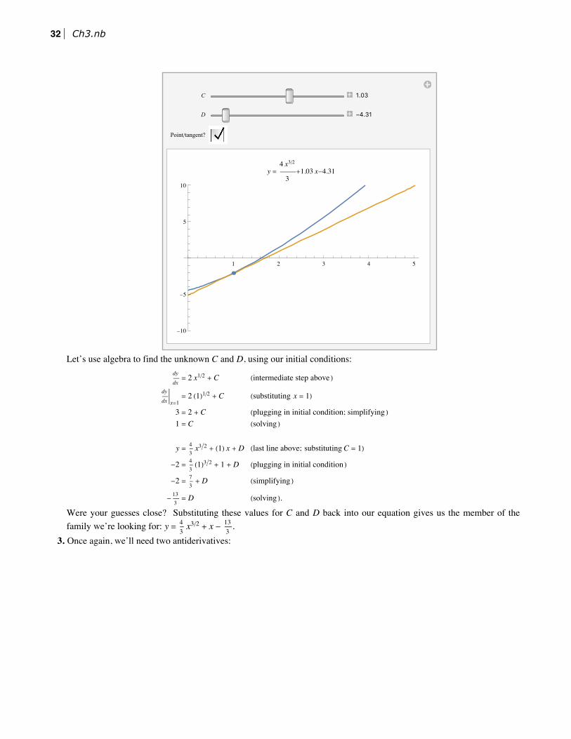
C 1.03
D -4.31
Point/tangent?
1 2 3 4 5
-10
-5
5
10
y =4 x3/2
3+1.03 x-4.31
Let’s use algebra to find the unknown C and D, using our initial conditions:dy
dx= 2 x1/2 + C (intermediate step above )
dy
dxx=1
= 2 (1)1/2 + C (substituting x = 1)
3 = 2 + C (plugging in initial condition; simplifying )1 = C (solving )
y = 43
x32 + (1) x + D (last line above; substituting C = 1)
-2 = 43(1)32 + 1 + D (plugging in initial condition )
-2 = 73+ D (simplifying )
- 133= D (solving ).
Were your guesses close? Substituting these values for C and D back into our equation gives us the member of thefamily we’re looking for: y = 4
3x3/2 + x - 13
3.
3. Once again, we’ll need two antiderivatives:d2 y
dx2 = x13 (arithmetic rules )
d2 y
dx2 dx = ∫ x13 dx (integrating both sides )
dy
dx= x4/3
43+ C (computing integrals )
dy
dx= 3
4x43 + C (simplifying )
dy
dxdx =
34
x43 + C dx (integrating both sides )
y = 34 x7/3
73 + C x + D (computing integrals )
= 928
x73 + C x + D (simplifying ).
32 Ch3.nb

d2 y
dx2 = x13 (arithmetic rules )
d2 y
dx2 dx = ∫ x13 dx (integrating both sides )
dy
dx= x4/3
43+ C (computing integrals )
dy
dx= 3
4x43 + C (simplifying )
dy
dxdx =
34
x43 + C dx (integrating both sides )
y = 34 x7/3
73 + C x + D (computing integrals )
= 928
x73 + C x + D (simplifying ).
This time, the initial conditions given are both values of the solution function itself; that means our solution must pass through the points(1, -2) and (8, 4). Here’s the graph of the family, with those points marked. Try to find values of C and D that make the graph pass throughthose points:
C -5.
D 2.53
2 4 6 8 10
-10
-5
5
10
y =9 x7/3
28-5.00 x+2.53
Once again, we’ll use algebra to find the actual values of the parameters C and D:
y = 928
x73 + C x + D (last line above )
-2 = 928
(1)73 + C (1) + D (plugging in point (1, -2))
-2 - 928
= C + D subtracting 928
- 6528
= C + D (simplifying )
4 = 928
(8)73 + C (8) + D (plugging point (8, 4) into solution )
4 = 928
(128) + 8 C + D (simplifying )
4 - 2887
= 8 C + D simplifying , subtracting 2887
- 2607
= 8 C + D (simplifying ).
Ch3.nb 33
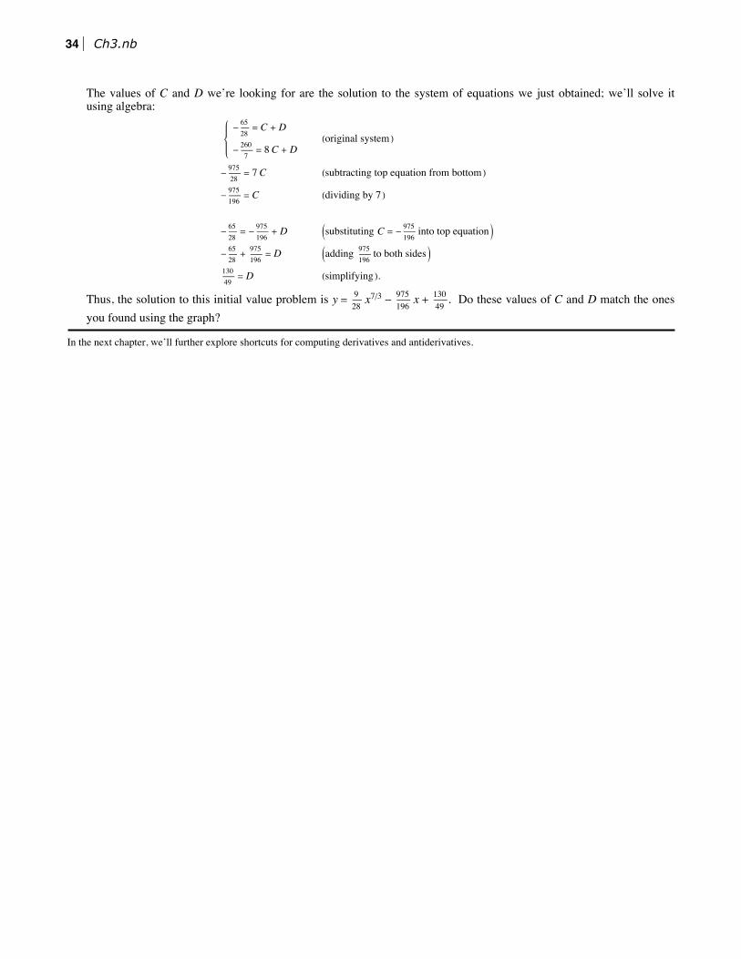
The values of C and D we’re looking for are the solution to the system of equations we just obtained; we’ll solve itusing algebra:
- 6528
= C + D
- 2607
= 8 C + D(original system )
- 97528
= 7 C (subtracting top equation from bottom )
- 975196
= C (dividing by 7 )
- 6528
= - 975196
+ D substituting C = - 975196
into top equation
- 6528
+ 975196
= D adding 975196
to both sides 13049
= D (simplifying ).
Thus, the solution to this initial value problem is y = 928
x7/3 - 975196
x + 13049
. Do these values of C and D match the onesyou found using the graph?
In the next chapter, we’ll further explore shortcuts for computing derivatives and antiderivatives.
34 Ch3.nb