CALCULATIONS & STATISTICS - Press Ganey 19 - Guide to... · CALCULATIONS & STATISTICS. GUIDE TO INTERPRETING 1 ... Calculation of Mean Scores ... In terms of your Press,

CALCULATIONS & STATISTICS

GUIDE TO INTERPRETING

1

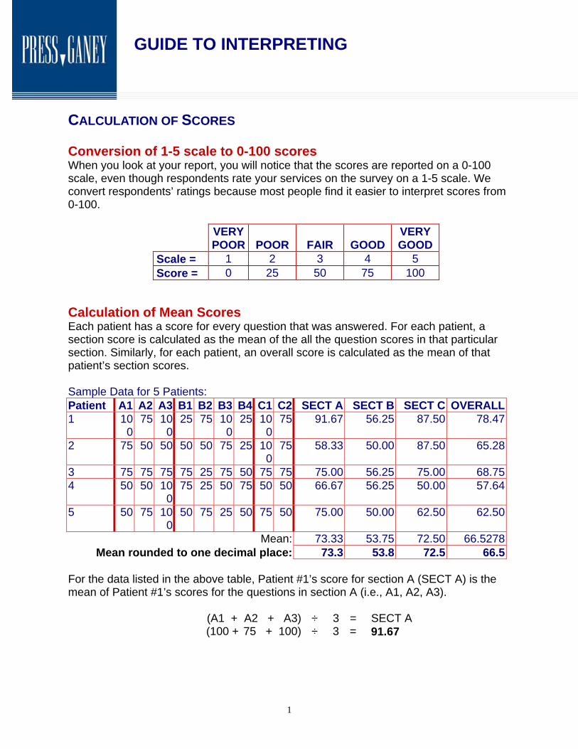
CALCULATION OF SCORES Conversion of 1-5 scale to 0-100 scores When you look at your report, you will notice that the scores are reported on a 0-100 scale, even though respondents rate your services on the survey on a 1-5 scale. We convert respondents’ ratings because most people find it easier to interpret scores from 0-100.

VERY

POOR

POOR

FAIR

GOODVERY GOOD

Scale = 1 2 3 4 5 Score = 0 25 50 75 100

Calculation of Mean Scores Each patient has a score for every question that was answered. For each patient, a section score is calculated as the mean of the all the question scores in that particular section. Similarly, for each patient, an overall score is calculated as the mean of that patient’s section scores.

Sample Data for 5 Patients: Patient A1 A2 A3 B1 B2 B3 B4 C1 C2 SECT A SECT B SECT C OVERALL1 10

0 75 10

0 25 75 10

025 10

075 91.67 56.25 87.50 78.47

2 75 50 50 50 50 75 25 100

75 58.33 50.00 87.50 65.28

3 75 75 75 75 25 75 50 75 75 75.00 56.25 75.00 68.754 50 50 10

0 75 25 50 75 50 50 66.67 56.25 50.00 57.64

5 50 75 100

50 75 25 50 75 50 75.00 50.00 62.50 62.50

Mean: 73.33 53.75 72.50 66.5278Mean rounded to one decimal place: 73.3 53.8 72.5 66.5

For the data listed in the above table, Patient #1’s score for section A (SECT A) is the mean of Patient #1’s scores for the questions in section A (i.e., A1, A2, A3).

(A1 + A2 + A3) ÷ 3 = SECT A (100 + 75 + 100) ÷ 3 = 91.67


2

Similarly, Patient #1’s OVERALL score is calculated: (SECT A + SECT B + SECTC) ÷ 3 = OVERALL (91.67 + 56.25 + 87.50) ÷ 3 = 78.47 The section scores displayed in a report are the means of all the patients’ scores for that section, rounded to one decimal place. (See bold face type at the bottom of SECT A, SECT B, and SECT C columns). Similarly, the overall facility rating score displayed in a report is the mean of all patients’ overall scores, rounded to one decimal place. (See bold face type at the bottom of OVERALL column).

(78.47 + 65.28 + 68.75 + 57.64 + 62.50)

÷ 5 = 66.5278 = 66.5

In a perfect world where every patient fills in every question, you could also calculate the overall hospital rating by taking the mean of the section averages displayed in your report.

(73.3 + 53.8 + 72.5) ÷ 3 = 66.5

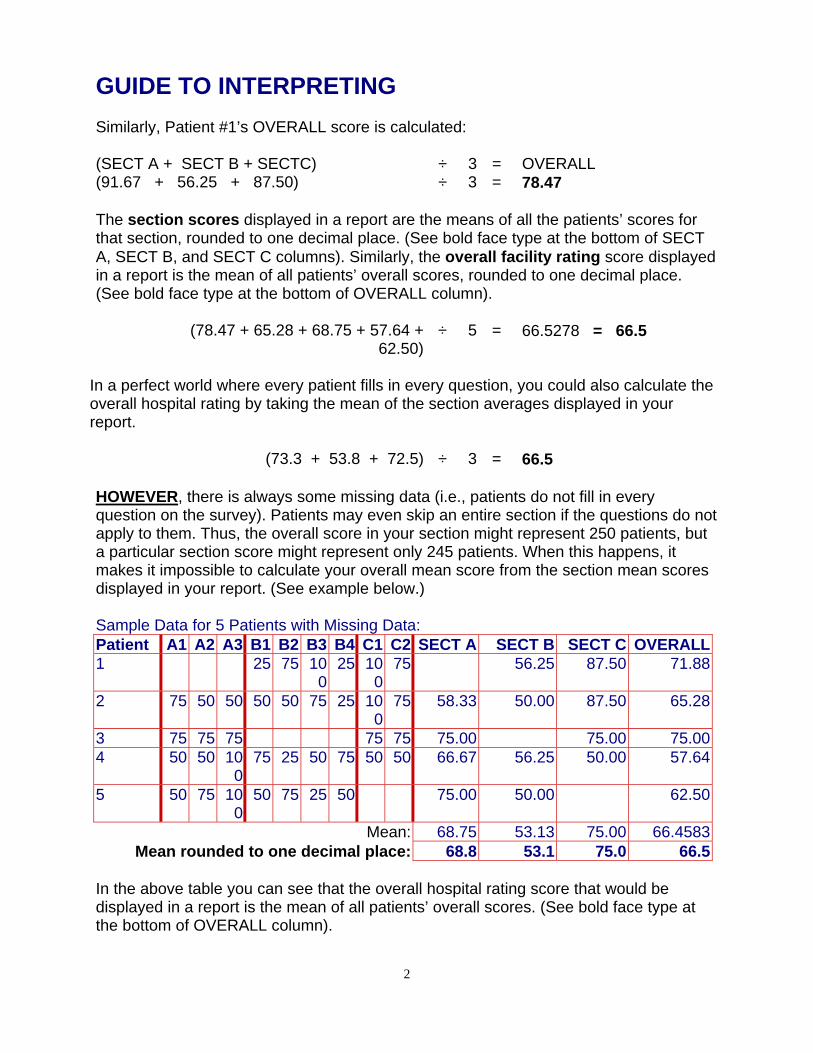
HOWEVER, there is always some missing data (i.e., patients do not fill in every question on the survey). Patients may even skip an entire section if the questions do not apply to them. Thus, the overall score in your section might represent 250 patients, but a particular section score might represent only 245 patients. When this happens, it makes it impossible to calculate your overall mean score from the section mean scores displayed in your report. (See example below.) Sample Data for 5 Patients with Missing Data: Patient A1 A2 A3 B1 B2 B3 B4 C1 C2 SECT A SECT B SECT C OVERALL1 25 75 10

025 10

075 56.25 87.50 71.88

2 75 50 50 50 50 75 25 100

75 58.33 50.00 87.50 65.28

3 75 75 75 75 75 75.00 75.00 75.004 50 50 10

0 75 25 50 75 50 50 66.67 56.25 50.00 57.64

5 50 75 100

50 75 25 50 75.00 50.00 62.50

Mean: 68.75 53.13 75.00 66.4583Mean rounded to one decimal place: 68.8 53.1 75.0 66.5

In the above table you can see that the overall hospital rating score that would be displayed in a report is the mean of all patients’ overall scores. (See bold face type at the bottom of OVERALL column).


3

(71.88 + 65.28 + 75.00 + 57.64 + 62.50) ÷ 5 = 66.4583 = 66.5

Because of missing data, you cannot obtain the overall hospital rating score by taking the mean of the section averages displayed in the report.

(68.8 + 53.1 + 75.0) ÷ 3 = 65.6333 = 65.6

Note: The difference appears small in this example because there are so few patients in the sample. In practice the difference would be much greater.

THE MEAN The Mean (denoted X, and referred to as x-bar) is a measure of central tendency representing the arithmetic center of a group of scores. In plainer language, it is the average. In terms of your Press, Ganey report, the mean gives you information about the average score for: an individual question, a section on the survey, the overall satisfaction score for your facility, or the satisfaction scores for all facilities in our database. The mean is calculated by summing all scores and dividing by the number of scores. For example, the mean of 88.0, 87.5, and 86.5 would be calculated:

(88.0 + 87.5 + 86.5) ÷ 3 = 87.33 A more general formula can be written:

The mean can also be interpreted as the balancing point. Each score can be thought of as a one pound weight and the range of values of scores could be plotted along a supporting rod. The balancing point for the rod would be the mean of the values of the scores. Interestingly, physicists determine the precise balancing point, or center of gravity, using the same formula that statisticians use to find the mean. ] ] ]

84.5 85.0 85.5 86.0 86.5 87.0 87.5 88.0 88.5 89.0 89.5 90.0

X 87.33

Mean X X X X ... X

n1 n2 3

= =+ + +


4

The mean, or balancing point, is easily influenced by outliers (i.e., scores that are much higher or much lower than the rest of the scores). If you put a weight on the balancing rod that was in about the same place as all the other weights (e.g., 87.0), the rod wouldn’t tip very much and you wouldn’t have to move the balancing point very far. If, however, you placed a weight way out on the end of the rod (e.g., 90.0), the rod would tip considerably. You would need to move the balancing point closer to the extreme value in order to make the rod balance. The same holds true with calculating the mean. If you have a group of scores that are all within a close range, the mean value will likely be towards the center of that range. However, having just one score that is much higher or lower than the rest can pull the mean up or down, respectively. Note: Remember that the mean score is an average, not a percent. Say you have a sample of five patients who rate ‘skill of nurses’ as follows: 5 (very good), 4 (good), 4 (good), 4 (good), 5 (very good). Those ratings can be converted into the following scores: 100, 75, 75, 75, 100. The average of these scores would be 85 ((100+75+75+75+100)÷5). You wouldn’t want to say that your patients were 85% satisfied with the skill of nurses, because in fact all (100%) of your patients rated the nurses good or very good with 60% giving a rating of good and 40% giving a rating of very good.

THE MEDIAN & PERCENTILE RANKING The Median The median is a measure of central tendency representing the mid-point in a distribution of scores or the point at the 50th percentile. In other words, the median is the middle; it is the score that splits the distribution in half. Fifty percent of scores will fall above the median and fifty percent of scores will fall below the median. The median is determined by ordering the scores from highest to lowest and finding the middle value. If there is an odd number of scores, the median is the score in the middle. If there is an even number of scores, then there is no score in the middle so the median is the average of the two scores closest to the middle. Comparison of the Mean and the Median The mean and the median are each measures of central tendency, but they describe the center in different ways. The mean is the average of the scores, whereas the median is the middle of the scores. The average is not always in the middle of a distribution. Another difference between the two is that the mean is influenced by outliers (i.e., scores that are much higher or lower than the rest) but the median is not influenced by outliers. To illustrate this point, let’s look at an imaginary sample of ten facilities’ overall satisfaction scores:


5

Hos # 1 69.4 Hos # 2 98.5 Finding the Mean: Hos # 3 84.6 The mean of these scores is obtained by summing the Hos # 4 87.1 scores and dividing by the number of scores (ten) to get

85. 9. Hos # 5 78.3 Hos # 6 93.3 Mean = (69.4 + 98.5 + 84.6 + 87.1 + 78.3 + Hos # 7 81.7 93.3 + 81.7 + 86.2 + 90.5 + 89.8) ÷10 Hos # 8 86.2 = 85.9 Hos # 9 90.5 Hos # 10 89.8

Hos # 2 98.5 Hos # 6 93.3 Finding the Median: Hos # 9 90.5 To find the median, the hospital scores are ordered from

highest Hos # 10 89.8 to lowest. In this case there is an even number of scores

so we Hos # 4 87.1 must take the average of the two closest to the middle

(i.e., 87.1 Hos # 8 86.2 and 86.2). Hos # 3 84.6 Hos # 7 81.7 Media

n = (87.1+ 86.2) ÷ 2

Hos # 5 78.3 = 86.65 Hos # 1 69.4

Notice the relationship between the mean and the median. In this example, the mean is lower than the median because an outlier (the low score of 69.5) pulled the mean down a bit. The low outlier did not influence the median. If you were facility # 8, with a score of 86.2, you would notice that your facility score is above the mean (85.9) for the database but below the median (86.65). The median for the database is equivalent to the 50th percentile in the percentile ranking, so facility #8 would be below the 50th percentile. So if your facility’s score is above the mean but below the 50th percentile it indicates that there are low outliers in the database (facilities whose score are considerably lower than all the other scores). Conversely, if your score is below the mean but above the 50th percentile, it indicates that there are high outliers in the database (facilities whose scores are considerably higher than all the other scores).

Percentile Ranking Percentile ranking is a strategy for assigning a series of values to divide a distribution into equal parts. More specifically, the percentile ranking tells you the proportion of scores in the database which fall below your individual facility’s score. The median of


6

the database is the score associated with the 50th percentile. Percentile rankings therefore give you information about where your hospital stands in relation to the median of the database. Keep in mind that these numbers are percentiles, not actual scores. For example, a 68 in the percentile rank column of your report means that the hospital is in the 68th percentile for this item. Translation: this particular hospital scores higher than 68% of the hospitals in the database and scores lower than 32 % of the hospitals in the database. For more information on percentile rankings please see the section on the Standard Deviation and the discussion of how percentile rankings relate to the standard deviation.

THE STANDARD DEVIATION & STANDARD ERROR (SIGMA)

What is the Standard Deviation? The standard deviation is a measure of variability of scores around the mean. Large numbers for the standard deviation indicate that the data are very spread out (i.e., there is a lot of variability). Conversely, a very small standard deviation would indicate that most of the data are very similar to the mean (i.e., less variability). How do you determine the Standard Deviation? The standard deviation is calculated using the formula:

In plainer terms, this formula tells you to (see example below):

Find the mean of the sample you are interested in (bottom cell of second column). Find the ‘distance from the mean’ for each individual score. You do this by

subtracting the mean from each hospital score (see third column). Square all the ‘distances from the mean’ (fourth column). Add all of the squared distances from the mean scores (bottom cell of fourth

column). Divide the sum of the squared distances by the number of scores you are working

with, (in this example, there are five scores). The number you get, 92.99 is called the variance.

Take the square root of your answer from number ...This is the Standard Deviation...9.64!

( )n

XX2

∑ −


7

Example 1

FACILITY SCORE (SCORE – MEAN) (SCORE – MEAN)2

X (X-X) (X-X)2 1 69.4 69.4 - 83.5

8= -

14.18201.07

2 98.5 98.5 - 83.58

= 14.92 222.61

3 84.6 84.6 - 83.58

= 1.02 1.04

4 87.1 87.1 - 83.58

= 3.52 12.39

5 78.3 78.3 - 83.58

= -5.28 27.88

464.99 ÷ 5 X Sum of (X-X)2 = 92.998 = 83.58 = 464.99 Square root of 92.998 =9.64

For comparison, a second example (Example 2) is provided that shows the computation of the standard deviation for a different set of five scores. Notice that the mean is the same as in the first example (83.58). However the standard deviation is considerably smaller (1.32) because the scores are much closer to the mean than were the scores in the first example. In other words, two sets of data with the same mean won’t necessarily be identical to one another.


8

Example 2 FACILITY SCORE (SCORE – MEAN) (SCORE – MEAN)2

X (X-X) (X-X)2 6 83.8 83.8 - 83.5

8= 0.22 0.05

7 82.5 82.5 - 83.58

= -1.08 1.17

8 84.6 84.6 - 83.58

= 1.02 1.04

9 81.7 81.7 - 83.58

= -1.88 3.53

10 85.3 85.3 - 83.58

= 1.72 2.96

X Sum of (X-X)2 8.75 ÷ 5 = 83.58 = 8.75 = 1.75 Square root of 1.75 =1.32

Importance of the Standard Deviation Knowing the standard deviation of the database is important because it allows you to compare your facility’s score to the larger group. We can do this based on the normal distribution. The normal distribution (below) is a bell shaped curve representing a theoretical distribution of data in which the mean, median, and mode (the score that occurs most frequently) have the same value. In the normal distribution 68% of all data falls within one standard deviation of the mean of the distribution. Further, 95% of the data falls within two standard deviations of the mean.

The Normal Distribution

-2 S.D. -1 S.D. X +1 S.D. +2 S.D.

68.26%

95.44%


9

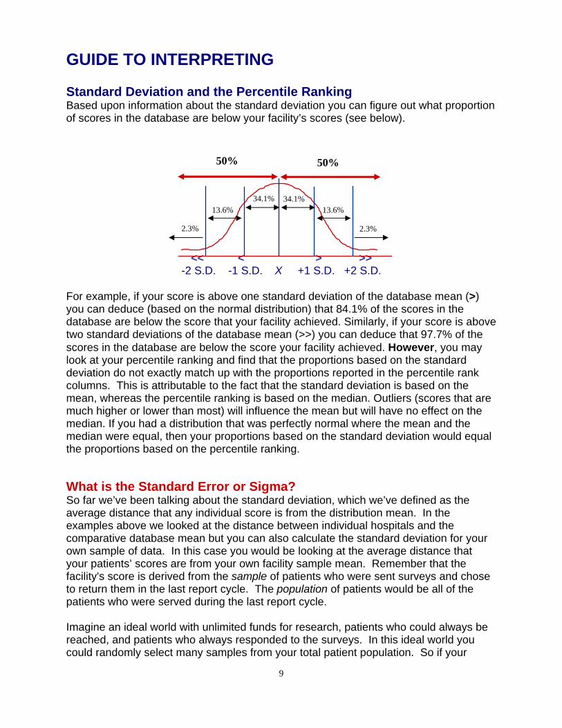
Standard Deviation and the Percentile Ranking Based upon information about the standard deviation you can figure out what proportion of scores in the database are below your facility’s scores (see below).

<< < > >> -2 S.D. -1 S.D. X +1 S.D. +2 S.D.

For example, if your score is above one standard deviation of the database mean (>) you can deduce (based on the normal distribution) that 84.1% of the scores in the database are below the score that your facility achieved. Similarly, if your score is above two standard deviations of the database mean (>>) you can deduce that 97.7% of the scores in the database are below the score your facility achieved. However, you may look at your percentile ranking and find that the proportions based on the standard deviation do not exactly match up with the proportions reported in the percentile rank columns. This is attributable to the fact that the standard deviation is based on the mean, whereas the percentile ranking is based on the median. Outliers (scores that are much higher or lower than most) will influence the mean but will have no effect on the median. If you had a distribution that was perfectly normal where the mean and the median were equal, then your proportions based on the standard deviation would equal the proportions based on the percentile ranking. What is the Standard Error or Sigma? So far we’ve been talking about the standard deviation, which we’ve defined as the average distance that any individual score is from the distribution mean. In the examples above we looked at the distance between individual hospitals and the comparative database mean but you can also calculate the standard deviation for your own sample of data. In this case you would be looking at the average distance that your patients’ scores are from your own facility sample mean. Remember that the facility's score is derived from the sample of patients who were sent surveys and chose to return them in the last report cycle. The population of patients would be all of the patients who were served during the last report cycle. Imagine an ideal world with unlimited funds for research, patients who could always be reached, and patients who always responded to the surveys. In this ideal world you could randomly select many samples from your total patient population. So if your

50% 50%

34.1% 34.1% 13.6% 13.6%

2.3% 2.3%


10

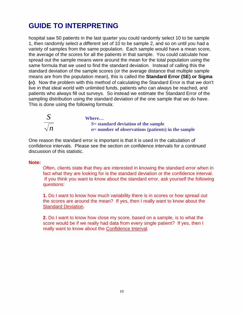
hospital saw 50 patients in the last quarter you could randomly select 10 to be sample 1, then randomly select a different set of 10 to be sample 2, and so on until you had a variety of samples from the same population. Each sample would have a mean score, the average of the scores for all the patients in that sample. You could calculate how spread out the sample means were around the mean for the total population using the same formula that we used to find the standard deviation. Instead of calling this the standard deviation of the sample scores (or the average distance that multiple sample means are from the population mean), this is called the Standard Error (SE) or Sigma (σ). Now the problem with this method of calculating the Standard Error is that we don’t live in that ideal world with unlimited funds, patients who can always be reached, and patients who always fill out surveys. So instead we estimate the Standard Error of the sampling distribution using the standard deviation of the one sample that we do have. This is done using the following formula:

nS

One reason the standard error is important is that it is used in the calculation of confidence intervals. Please see the section on confidence intervals for a continued discussion of this statistic. Note:

Often, clients state that they are interested in knowing the standard error when in fact what they are looking for is the standard deviation or the confidence interval. If you think you want to know about the standard error, ask yourself the following questions:

1. Do I want to know how much variability there is in scores or how spread out the scores are around the mean? If yes, then I really want to know about the Standard Deviation. 2. Do I want to know how close my score, based on a sample, is to what the score would be if we really had data from every single patient? If yes, then I really want to know about the Confidence Interval.

Where… S= standard deviation of the sample n= number of observations (patients) in the sample


11

CONFIDENCE INTERVAL

What is a Confidence Interval? The confidence interval is the region in which a population score is likely to be found. In other words, it is the range around your sample mean in which you would expect to find your true population mean. When looking at the mean for a sample of a population, you get a very good estimate of the mean for the whole population, but you don’t come up with the exact number. The only way you could truly know the true population mean is if you actually had data from everyone in the population (i.e., every single patient at your facility received and completed a survey). The mean score that you get for the sample of patients who returned the surveys is an accurate reflection of the opinions of those in the sample and is considered to be an estimate of the score that would characterize the whole population. The confidence interval tells you the range of values, around your sample mean, that would be expected to contain the mean for the actual population. For example, if your sample mean is 80 and your confidence interval is 2 then you would say that the estimate for the mean of your entire patient population is 80 + 2 which would be 78-82. So the confidence interval answers the question: What is the range of values around our sample mean that we are 95% sure contains the actual population mean? How do you calculate a confidence interval? A 95% confidence interval is calculated using the following formula:

( )XSEXIC 96.1.. ±=

Which is read as the sample mean plus or minus 1.96 times the standard error. Remember that if you wanted to know where 95% of your patients’ scores were, you could take your sample mean plus or minus two standard deviations. Calculating a confidence interval uses the same logic but applies it differently. For the confidence interval we are not trying to find a range within a sample that contains 95% of scores, but the range within a population that contains 95% of sample mean scores. The standard error (SE) tells you the average distance that a sample mean would be from the population mean (see discussion of the SE in the section on standard deviations); it’s like saying the standard deviation of the sample means around the population mean. We could just find the interval that is plus or minus two standard errors (like we do with the standard deviation). However, if you remember from the picture of the normal distribution, two standard deviations actually gives you slightly more than 95%. It gives you 95.44 %. If we want to know exactly 95%, then we would want slightly less than two standard errors ⎯ 1.96.


12

One last issue. We don’t know the exact standard error of the population because we don’t have multiple samples drawn from the same population at the same time. We have just one sample from the population. However, we can estimate the standard error of the population based on the standard deviation of our one sample using the following formula:

nS

So if a facility had an overall rating of 84.24 with a standard deviation of 4.5 and an n of 225 we could calculate the standard error as...

63.0225

5.9===

nSSE

And the confidence interval would be calculated ...

( ) ( ) 24.124.8463.096.124.8496.1.. ±=±=±= XSEXIC Thus, with a sample mean of 84.24, we are 95% confident that the actual population mean is between 83.00 and 85.48. Note:

The Confidence Intervals that are listed in your report under the heading Facility Statistical Analysis can be used to estimate the amount of change in mean score you would need in order to show a statistically significant improvement. In order to create this estimate you must multiply the number in the 95% Confidence Interval column by 1.41 and add the result to your current mean. So, if you had a mean of 84.24 and confidence interval of 1.24 you could estimate that increasing your mean score by multiplying the 1.24 by 1.41. The result, 1.75, is an estimate of how much you would have to increase your mean score (i.e., from 84.24 to 85.99). This estimate is a just a guide and assumes that your sample for the next report has exactly the same n and standard deviation as the data for the current report.

Where… S= standard deviation of the sample n= number of observations (patients) in the sample


13

t-TESTS The statistical procedure used to determine if scores on a current report are significantly different from the scores on the last report is the t-test. The calculation of a t-test measures the difference between sample means, taking into account the size and variability of each of the samples. It is important to note that the result of the t-test does not simply tell you what the difference is, it tells you how confident you can be that the difference is real and not due to random error. Conventionally, if you are at least 95% confident that the difference is real and thus not due to random error, then the difference is said to be statistically significant. How do you calculate a t-test? t-tests are calculated using the following formula...

( )

2

22

1

21

21

nS

nS

XXt+

−=

X1 = the mean of sample 1

X2 = the mean of sample 2

S1

2 = the variance (Stand. Dev.2 ) of sample 1

S2

2 the variance (Stand. Dev.2 ) of sample 2

n1 = the number of observations in sample 1

n2 = the number of observations in sample 2

In your report... When a score on a Press, Ganey report is found to be significantly different from the score on the last report, the score is highlighted with one of the following symbols:

+ 95% certainty of significant increase (t >1.96). + + 99% certainty of significant increase (t >2.576). - 95% certainty of significant decrease (t< -1.96). - - 99% certainty of significant decrease (t< -2.576).

Two factors can influence whether or not a difference is found to be significant: the size of the samples (n) and the variability of the samples. Size: It is less likely that you will be confident enough to call a difference significant (i.e., not due to error) if there is less data available (lower n’s). Variability: It is less likely that you will be confident enough to call a difference significant (i.e., not due to error) when there is greater variability (i.e., the data are more


14

spread out around the mean of the sample; larger standard deviations). So if you have what appear to be large differences in scores that are not marked with an indicator of statistically significant difference, it is likely that either the n’s were too low or the standard deviations were too large for you to be confident that the difference was real and not due to random error. Conversely, if you have what appear to be small differences in scores that are marked with an indicator of statistically significant difference, it is likely that either the n’s were so high or the standard deviation was so small that it was possible to be very confident that the difference was real and not due to random error. How can we be sure that differences in scores are significant at the .05 level, especially when sample sizes are small? ** Remember that a t-test takes into account both the size of the samples and the variability of the samples, so if the results of a t-test indicate that a difference is indeed significant, then you can be at least 95% confident that the difference is real and not due to random error, no matter how small your samples are.


15

CORRELATIONS What is a correlation? A correlation tells you the strength of the relation between variables. In other words, a correlation tells us how much a change in one variable (e.g., a question score) is associated with a concurrent, systematic change in another variable (e.g., overall satisfaction). A correlation represents the strength of the relationship between two variables numerically, with a correlation coefficient (called r) which can range from -1.0 to + 1.0. A positive correlation coefficient indicates that as the value of one variable increases, the value of the other variable also increases. For example, the more you exercise, the greater your endurance. A negative correlation coefficient indicates that as the value of one variable increases the value of the other variable decreases. For example, the more you smoke cigarettes, the less lung capacity you have. It is important to recognize that when two variables are correlated it means that they are related to each other, but it does not necessarily mean that one variable influences or predicts the other. This is the basis of the statement, “Correlation does not imply causation!” How can you tell how strong the relationship is between two variables?

• The closer a correlation is to 1 (either positive or negative), the stronger the relationship.

• The closer a correlation is to 0 (either positive or negative), the weaker the relationship.

How is a correlation calculated? Correlation coefficients are calculated using the formula below. This statistic basically assesses the degree to which variables X and Y vary together (the numerator) taking into account the degree to which each variable varies on its own (the denominator).

∑∑∑=

22 yxxyr

Example of calculating the correlation between... X (Overall rating of care provided at this facility) and Y (Likelihood of recommending this hospital). Please see the table on the following page.


16

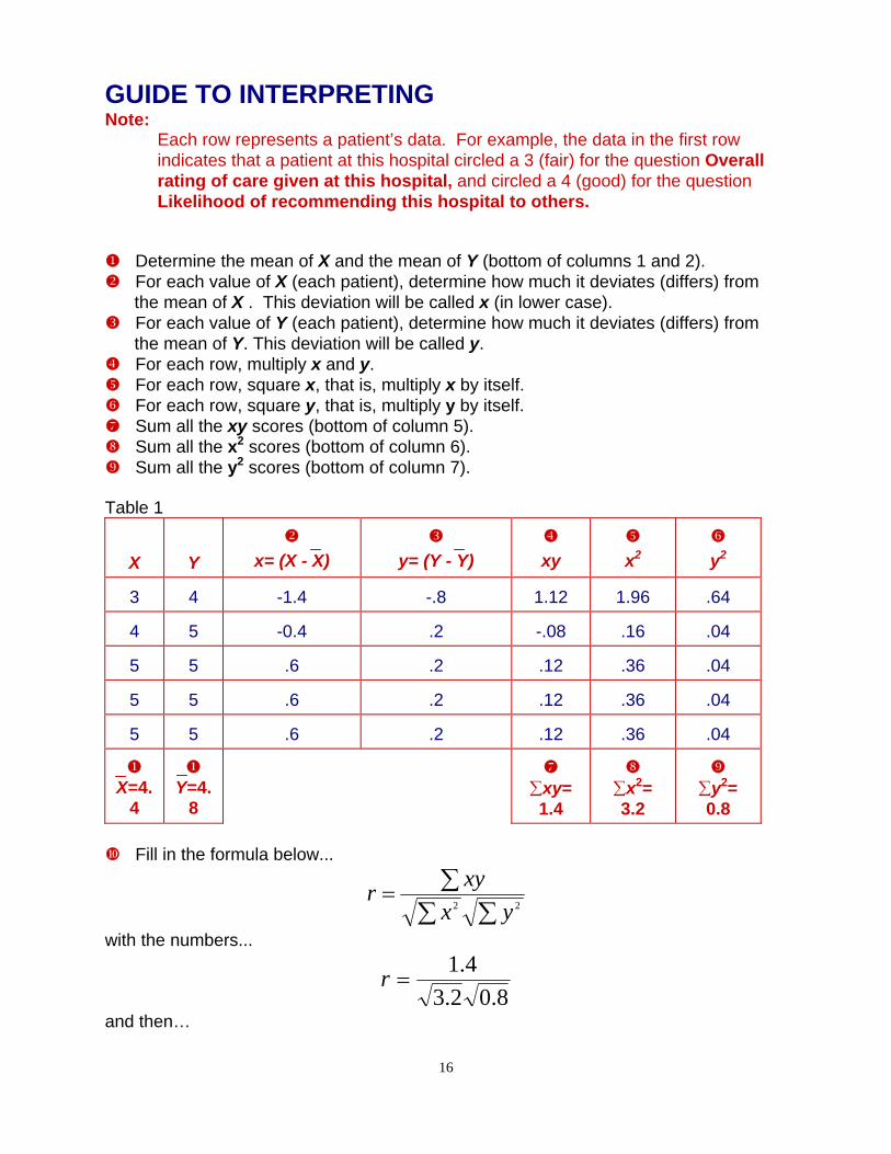
Note: Each row represents a patient’s data. For example, the data in the first row indicates that a patient at this hospital circled a 3 (fair) for the question Overall rating of care given at this hospital, and circled a 4 (good) for the question Likelihood of recommending this hospital to others.

Determine the mean of X and the mean of Y (bottom of columns 1 and 2). For each value of X (each patient), determine how much it deviates (differs) from

the mean of X . This deviation will be called x (in lower case). For each value of Y (each patient), determine how much it deviates (differs) from

the mean of Y. This deviation will be called y. For each row, multiply x and y. For each row, square x, that is, multiply x by itself. For each row, square y, that is, multiply y by itself. Sum all the xy scores (bottom of column 5). Sum all the x2 scores (bottom of column 6). Sum all the y2 scores (bottom of column 7).

Table 1

X

Y

x= (X - X)

y= (Y - Y)

xy

x2

y2

3

4

-1.4

-.8

1.12

1.96

.64

4

5

-0.4

.2

-.08

.16

.04

5

5

.6

.2

.12

.36

.04

5

5

.6

.2

.12

.36

.04

5

5

.6

.2

.12

.36

.04

X=4.

4

Y=4.8

∑xy= 1.4

∑x2= 3.2

∑y2= 0.8

Fill in the formula below...

∑∑∑=

22 yxxyr

with the numbers...

8.02.34.1

=r

and then…


17

89.0*79.14.1

=r

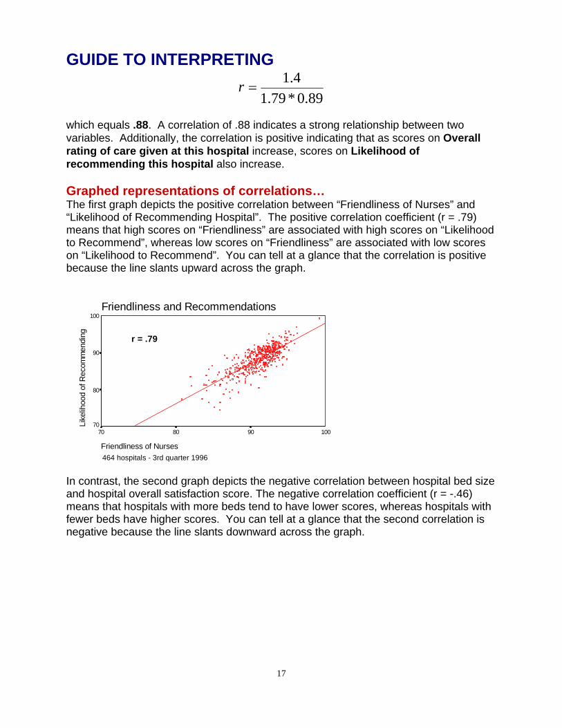
which equals .88. A correlation of .88 indicates a strong relationship between two variables. Additionally, the correlation is positive indicating that as scores on Overall rating of care given at this hospital increase, scores on Likelihood of recommending this hospital also increase. Graphed representations of correlations… The first graph depicts the positive correlation between “Friendliness of Nurses” and “Likelihood of Recommending Hospital”. The positive correlation coefficient (r = .79) means that high scores on “Friendliness” are associated with high scores on “Likelihood to Recommend”, whereas low scores on “Friendliness” are associated with low scores on “Likelihood to Recommend”. You can tell at a glance that the correlation is positive because the line slants upward across the graph.

Friendliness and Recommendations

Friendliness of Nurses

100908070

Like

lihoo

d of

Rec

omm

endi

ng

100

90

80

70

r = .79

464 hospitals - 3rd quarter 1996

In contrast, the second graph depicts the negative correlation between hospital bed size and hospital overall satisfaction score. The negative correlation coefficient (r = -.46) means that hospitals with more beds tend to have lower scores, whereas hospitals with fewer beds have higher scores. You can tell at a glance that the second correlation is negative because the line slants downward across the graph.


18

Overall Mean by Bed Size

Total Facility Beds

1400120010008006004002000

Aver

age

Com

mon

Que

stio

n M

ean

- 199

3

10000

9000

8000

7000

r = - .46

.

.

.

.

Regression vs. Correlation Press, Ganey reports list correlation coefficients between each question and the overall satisfaction score (an average of all the other items in a questionnaire). This gives a measure of the relative importance of each individual question for overall satisfaction. Clients sometimes ask why we do not use multiple regression to demonstrate these relationships. When the items of a survey are highly correlated, it is impossible to separate the effect of one item from that of others with any degree of precision. Because this problem (termed “multicollinearity”) violates one of the assumptions of multiple regression, Press, Ganey does not report multiple regression analyses performed to relate specific questions to overall satisfaction. Like regression analyses, correlations are statistical measures of association that describe the strength of relationship, or association, between factors, such as a doctor’s courtesy and patients’ overall satisfaction with care from that physician. Correlations have the advantage of using all the information from each respondent to a survey, whereas regression analyses eliminates all information from any respondents who do not answer every question.


19

PRIORITY INDEX

What is the priority index? The priority index is a way of combining two very important pieces of information: (1) the actual score achieved on a particular question, and (2) the degree to which that particular question is associated with overall satisfaction. Combining these two pieces of information helps a facility to know where efforts should be placed for quality improvement. For example, one question might be very low in score (e.g., quality of food) but not particularly associated with overall satisfaction. Because it is not highly associated with satisfaction the facility might chose to place quality improvement resources elsewhere. Conversely, a question might be very highly associated with overall satisfaction (e.g., overall cheerfulness of hospital) but not low in score. Attempting to raise the score would probably be difficult and may perhaps be unnecessary if most of your patients are very satisfied already. How is the priority index calculated? The priority index is derived through a three-step process. For the purpose of this example, let’s assume that the survey has 50 questions. 1. SCORE RANK Questions are ordered from the highest score down to the lowest score. Each question is then given a score rank; the highest mean score gets a rank of 1, the second highest score gets a rank of 2, the third highest score gets a rank of 3 and so on down the line until the lowest score is given a rank of 50. It may help to remember the meaning of the score rank to think of a high score as a small issue and a low score as a big issue--something the facility should be concerned about. The high score, a small issue, has a small score rank (e.g., 1, 2 , 3..). Conversely, a low score, a big issue of concern, has a big score rank (e.g., 48, 49, 50). The score rank for each question appears in parentheses to the right of the mean score column on the priority index page. 2. CORRELATION RANK Next, questions are ordered from the least correlated with overall satisfaction to the most associated with overall satisfaction. Each question is then given a correlation rank. The question that is the least correlated with satisfaction gets a rank of 1, the question that is the second least correlated with satisfaction gets a rank of 2 and so on down the line until the question that is the most correlated with satisfaction gets a rank of 50. Again, it helps to keep in mind what would be a small issue and what would be a big issue. A question that is not very correlated with satisfaction would be a small issue so it would have a small rank (e.g., 1, 2, 3...), whereas a question that was highly correlated with satisfaction would be a big issue--something to pay attention to--and would have a big rank (e.g. 48, 49, 50). The correlation rank for each question appears in parentheses to the right of the correlation coefficient column on the priority index page.


20

3. COMPUTING THE PRIORITY INDEX The priority index is derived by adding the score rank (from step 1) to the correlation rank (from step 2). The questions are then ordered on the priority index page with the largest priority index score coming first on down to the lowest priority index score coming last. In order to be first in the priority index list a question would have to have two big issues: a big score rank (that means a low score) and a big correlation rank (that means a high association with satisfaction). Questions that appear at the bottom of the priority index list would have two small issues, a high overall score (which gets a small score rank) and a low association with satisfaction (which gets a small correlation rank). Questions that appear in the middle of the priority index list would likely have just one big issue (either a low score or a high association with satisfaction).

PRIORITY

INDEX

=

SCORE RANK

+

CORRELATION RANK

High Priority

(Top of priority index page)

=A big issue!

Big score rank (Low actual score)

+

A big issue! Big correlation rank (High correlation with

satisfaction)

Medium Priority (Middle of priority index

page)

=A big issue!

Big score rank (Low actual score)

+A small issue

Small correlation rank (Low correlation with

satisfaction)

or A small issue

Small score rank (High actual

score)

+A big issue!

Big correlation rank (High correlation with

satisfaction)

Low Priority (Bottom of priority index

page)

=A small issue

Small score rank (High actual score)

+ A small issue Small correlation rank

(Low correlation with satisfaction)

External Priority Indices Priority indexes are also provided with an external focus. The internal priority index, as described above, uses your question mean scores as an internal measure of performance. The external priority indices use your question percentile ranks as an external measure of performance. The same basic steps are used to create the external priority indices. However, in the first step, the questions are ranked according to their percentile ranks (highest to lowest) instead of according to their mean scores.

Documents

CALCULATIONS & STATISTICS - Press Ganey 19 - Guide to... · CALCULATIONS & STATISTICS. GUIDE TO INTERPRETING 1 ... Calculation of Mean Scores ... In terms of your Press,