1

Calculation of Minimum Miscibility Pressure Using Fast Slimtube Simulation

Wei Yan, Michael L. Michelsen, Erling H. Stenby

Center for Energy Resources Engineering, Technical University of Denmark This paper was originally presented as SPE 153758 at the Eighteenth SPE Improved Oil Recovery Symposium held in Tulsa, Oklahoma, USA, 14–18 April 2012.

Abstract Minimum misciblility pressure (MMP) is a critical parameter in designing a miscible gas injection process. It is expected that 100% displacement efficiency on the microscopic scale can be achieved provided the injection pressure is above MMP. Two approaches are usually employed for equation of state (EoS) based MMP calculation. The slimtube simulation approach is a numerical simulation of the physical slimtube experiment, which is commonly accepted as the most reliable experimental method for MMP determination. This approach carries out slimtube simulation runs at a series of pressures and determines the MMP from the recovery-pressure curve, just as in the experiment. The global approach, which is based on the method of characteristics analysis of 1D gas injection, finds the MMP by locating the pressure where a key tie-line becomes critical. Although the global approach is faster, the slimtube approach is still a necessary complementary method especially when the injection process involves complex phase behavior caused by CO2 or heavy oils. This study addresses how to improve the computational efficiency of slimtube simulation for MMP calculation. Firstly, a robust and efficient algorithm for rigorous flash forms the basis of the whole strategy. Secondly, a tie-line distance based approximation (TDBA) method has been introduced on top of the rigorous algorithm. In the TDBA method, if a new feed composition in a grid block is close enough to a tie-line previously calculated in the same block, the previous tie-line results can be used with slight adjustment. The approximation affects the final recovery very little but greatly increases the speed. Thirdly, a higher order method can be employed to use a fewer number of grid blocks to get the same accuracy in recovery. Finally, a MMP search strategy is proposed to reduce the number of slimtube simulations needed. In addition, it is also discussed how to parallelize slimtube simulations for modern computers with multiple CPU cores to further chop the computation time. 1. Introduction Gas injection, a widely used enhanced oil recovey method, will probably play a more important role in the future due to several reasons: (1) gas injection is effective to recover residual oils and its application is likely to be promoted by higher oil prices; (2) for deeper reservoirs and particularly offshore deeper reservoirs, gas injection as a means to achieve a higher oil recovery can be crucial to viability of a project; (3) when combined with CO2 capture, gas injection can be used as a way to mitigate CO2 emission. During gas injection, the injected gas will swell the oil, reduce oil viscosity, and most importantly, achieve miscibility by exchanging components with the oil. The extent of miscibility increases with pressure, and the threshold pressure above which the injected gas becomes completely miscible with the oil is known as the minimum miscibility pressure (MMP). Above the MMP, 100% displacement efficiency can be expected on the microscopic scale.

Development of miscibility between gas and oil is a dynamic process. In a 1-D conceptual picture, the injected gas keeps exchanging components with the reservoir fluid as it flows through the oil. The miscibility is a combined effect of local phase equilibrium and flow of the equilibrium phases—although recent studies show that the MMP is not influenced by the mobility ratio between gas and oil. Early explanations of miscibility always use pseudoternary phase diagrams where the fluid system is classified into three pseudo components: a gas component, an intermediate component, and an oil component. This conceptual model is useful to illustrate vaporizing gas drive (VGD) and condensing gas drive (CGD). In VGD, the injection gas becomes gradually enriched by extracting intermediate components from the reservoir oil and the miscibility is achieved at the displacement front between the enriched injection gas and the original reservoir oil. In CGD, the injection gas continuously enriches the reservoir oil by transferring the intermediate components to the oil and the miscibility is achieved near the injection well between the enriched reservoir fluid and the injection gas. However, the actual miscibility development can be more complex than pure vaporizing or condensing. This was revealed by Zick (1986) who showed that many gas injection systems involve both vaporizing and condensing processes. The combined condensing/vaporizing (C/V) mechanism can no longer be represented by a pseudo ternary phase diagram. The MMP due to a C/V mechanism can be significantly lower than that due to a VGD or CGD mechanism (Zick, 1986). Zick also pointed out that for multicomponent reservoir fluid systems it is not practical to achieve a CGD type miscibility.

MMP can be determined in the laboratory by a slimtube experiment. The experiment consists of gas injection at a series of pressures into the reservoir oil in a long slimtube packed with sand or glass beads. Each run at a pressure provides a correponding recovery at 1.2 PVI (pore volume injected) for this 1-D gas injection process. The MMP is usually determined as

2

the break point on the recovery-pressure plot. The experiment is time consuming but there are no other easy and reliable experimental methods to substitute it.

Different methods have been proposed for MMP calculations with an equation of state (EoS). The first type is the single-cell approach where the VGD or CGD mechanism is simulated by forward or backward contact in a single cell (Jensen and Michelsen, 1990). The minimum threshold pressure where multiple contacts just lead to a single phase result is interpreted as the MMP. Determination of the MMP using the single-cell approach is equivalent to searching the pressure where the initial tie-line or the injection tie-line becomes critical. The method does not account for the C/V mechanism and is therefore of limited use. The second type is to simulate the slimtube experiment using either a multicell simulator or a 1-D numerical simulator. The earliest attempts in this direction can be traced back to Cook et al. (1969) and Metcalfe et al. (1973). Cook et al. (1969) suggested using 20 cells as a simplified 1-D reservoir model. A computer program was developed to simulate oil vaporization during gas cycling in a linear laboratory-model oil reservoir. Metcalfe et al. (1973) extended the model of Cook et al. to study miscibility development rather than gas cycling. Metcalfe et al. gave a more sophisticated description on how to move gas and oil from one cell to the next. In addition to the “stagnant oil” option used by Cook et al., they also introduced two other options, namely moving excess oil and moving oil and gas according to their phase mobilities. The work of Metcalfe et al. forms the basis for later studies on miscibility using the multicell approach, such as the work of Pedersen et al. (1986). In parallel to the multicell approach is the 1-D compositional simulation approach used by Stalkup (1987). Stalkup proposed to study the 1-D displacement behavior with a compositional simulator. He noticed that the mixing caused by numerical dispersion can be larger than the mixing caused by physical dispersion. To remove the artificial dispersion, he suggested extrapolating the recovery to infinite small grid block size using a plot of the recovery versus 1/N0.5, where N is the number of grid blocks. Stalkup (1990) and Stalkup and Dean (1990) further investigated the effect of numerical dispersion and the sensitivity of gridding in finite difference (FD) simulations of the gas injection process, where extrapolation using 1/N was tried. Although appearing to be two different approaches, the multicell approach (also known as the multiple mixing cell simulation or the cell-to-cell simulation) and the 1-D FD simulation approach are actually based on the same formulation for 1-D gas injection. The former provides a physical interpretation of the 1-D gas injection process while the latter provides a mathematical solution to the problem (Jessen, 2000). The equivalence between a cell-to-cell simulation and an implicit single point upstream FD scheme was also implicated in the study of Michelsen (1998). Here, we put both the multicell approach and the 1-D FD approach under the same “slimtube simulation” category since they essentially simulate slimtube experiments. Høier and Whitson (2001) made a comphrensive study of different slimtube simulation algorithms, including Zick’s multicell algorithm. According to Høier and Whitson (2001), Zick’s algorithm is similar to the multicell approach proposed by Cook et al. and Metcalfe et al. However, Zick tracks the development of miscibility with a physical parameter, such as the difference of phase densities, which describes the distance from the critical point in each cell. The minimum of this physical parameter in each cell is extrapolated to the infinite grid number to get its dispersion free value. The MMP is searched by an automated code to locate where the distance parameter becomes zero. Høier and Whitson evaluated that the code was 20 to 100 times faster than multiple slimtube simulations. Jaubert et al. (1998a, 1998b) proposed a multicell algorithm to compute the MMP for any types of miscibility mechanisms. Their approach is essentially the same as that of Metcalfe et al. but with a few improvements for faster MMP calculation, such as extrapolating the recovery at infinite cells with a single simulation run, setting the pressure search region by the saturation pressure and the first contact miscibility pressure, and determinating MMP as the pressure corresponding to a recovery of 97% on the exponential curve fitted to the recoveries at different pressures. Metcalfe’s multicell approach was also used by Zhao et al. (2006) to illustrate that neither the ratio between injected gas and the oil at each batch nor the fluid mobility affects the MMP. Recently, Ahmadi and Johns (2008) proposed a different multiple mixing-cell method for MMP calculations. In their method, the mixing starts with only one gas cell and one oil cell, and continues to any number of cells that satisfy a desired accuracy. The transfer of gas and oil between cells has been largely simplified in this method. The third type of MMP calculation methods is based on the 1-D analytical theory of gas injection. Analysis of 1-D two-phase gas injection problems using the method of characteristics (MOC) shows that in addition to the initial tie-line and the injection tie-line, there exists a third key tie-line called the cross-over tie-line for a quaternary system (Monroe et al., 1990). Orr et al. (1993) showed that the multicomponent miscibility happens when a key tie-line becomes critical. In general, for a nc component gas injection systems, there exist nc-1 key tie-lines if the solution consists only of shocks, including the initial tie-line, the injection tie-line, and nc-3 cross over tie-lines. The key tie-lines will intersect pairwise for solutions consisting only of shocks. The intersecting key tie-lines are also a good approximation for practical MMP calculation (Wang and Orr, 1998). The intersecting key tie-lines was used to study MMP for a four-component system (Dindoruk, 1992) and later extended to fluid with 11 components (Johns and Orr, 1996). Wang and Orr (1997) proposed the first general algorithm for multi-component systems which also allows injection gas with more than one component. Jessen et al. (1998) substaintially increased the speed of MMP calculation for gas injection systems with an arbitrary number of components in either oil or gas. Details on the 1-D analytical theory of gas injection and their applications can be found in Orr’s book (Orr, 2007).

The purpose of this study is to speed up slimtube simulations for MMP determination. First, we review the mathematic formulation of the 1-D gas injection problem and present different numerical schemes for the problem. We then present a comprensive strategy to improve the simulation speed. Fast MMP determination using slimtube simulation depends on several factors including an efficient thermodynamic algorithm, appropriate approximation in flash calculations to cut simulation time, application of a higher order method to reduce numerical dispersion, and a proper MMP searching stategy to reduce the

3

number of required slimtube simulations. In addition, the advance in computer hardware can be utilized to parallelize slimtube simulations. The proposed algorithm was tested with 18 gas injection systems and the results are compared with those from the MOC approach. 2. Mathematical formulation and physical interpretation of slimtube simulation In the literature, 1-D FD simulation is often distinguished from multicell simulation. There are some arguments supporting this distinction. 1-D FD simulation can employ an existing compositional simulator and can include more details, such as pressure solution, capillary effects, dispersion effects, and realistic relative permeability models. In contrast, multicell simulation usually uses a tailor-made simulator where pressure is assumed constant, capillary and dispersion effects are neglected, and a simple fractional flow function is adopted. These differences, however, are not essential since one can easily simplify the 1-D FD simulation or complicate the multicell simulation. The two types of simulation are based on the same mathematic formulation as outlined in Section 2.1. The multicell simulation stresses more on the physical interpretation of the process while the 1-D FD simulation seeks to solve the problem from a mathematical point of view. The equivalence between a cell-to-cell simulation and an implicit SPU scheme is discussed in Section 2.2. And the similarity between Ahmadi and John’s multicell approach and an ESPU scheme is discussed in Section 2.3. In this study, we use slimtube simulation as a general name for both multicell simulation and 1-D FD simulation. 2.1. Governing equations for 1-D gas injection

For 1-D horizontal gas injection under the assumptions of non-deformable porous media, no capillary effects, and negligible dispersion and diffusion effects, the mass conservation equations are given by

011

=

∂∂

+

∂∂ ∑∑

==

pp n

jjjij

n

jjjij fxv

xsx

tρρφ 1, , ci n= (1)

or

0i iC Fτ ξ

∂ ∂+ =

∂ ∂ 1, , ci n= (2)

with dimensionless time τ and dimensionless distance ξ defined as

PVILtvinj ==

φτ (3)

xL

ξ = (4)

In Eqs.(2), Ci is the overall molar density of component i and Fi is the overall molar flux of component i:

1( )

pn

i i ij j jj

C C x sρ=

= =∑z (5)

1( , )

pn

i i D D ij j jj

F F v v x fρ=

= = ∑z (6)

The dimensionless velocity vD is defined as

injD v

vv = (7)

It is usually assumed that the gas injection is isothermal and local mass transfer is quick enough to reach instantaneous phase equilibrium. Phase equilibrium constraints and Eqs.(2) thus constitute the underlying equations for 1-D gas injection. The phase equilibrium part can be solved by isothermal flash, and Eqs.(2) can be solved using different numerical schemes. For finite difference methods, one can employ an implicit single point upstream (SPU) scheme, an expliit SPU method, or a higher order explicit method with Total Variation Diminishing (TVD) limitation. 2.2. Implicit SPU scheme

The implicit SPU (ISPU) discretization of Eqs.(2) is given by

4

1 * 1 * 1, , , , , 1 , 1( ) ( ) 0n n n n

i k i k D k i k D k i kC C v F v Fλ+ + +− −− + − = (8)

or in a vector form 1 * 1 * 1

, , 1 1n n n nk D k k k D k kv vλ λ+ + +

− −+ = +C F C F (9)

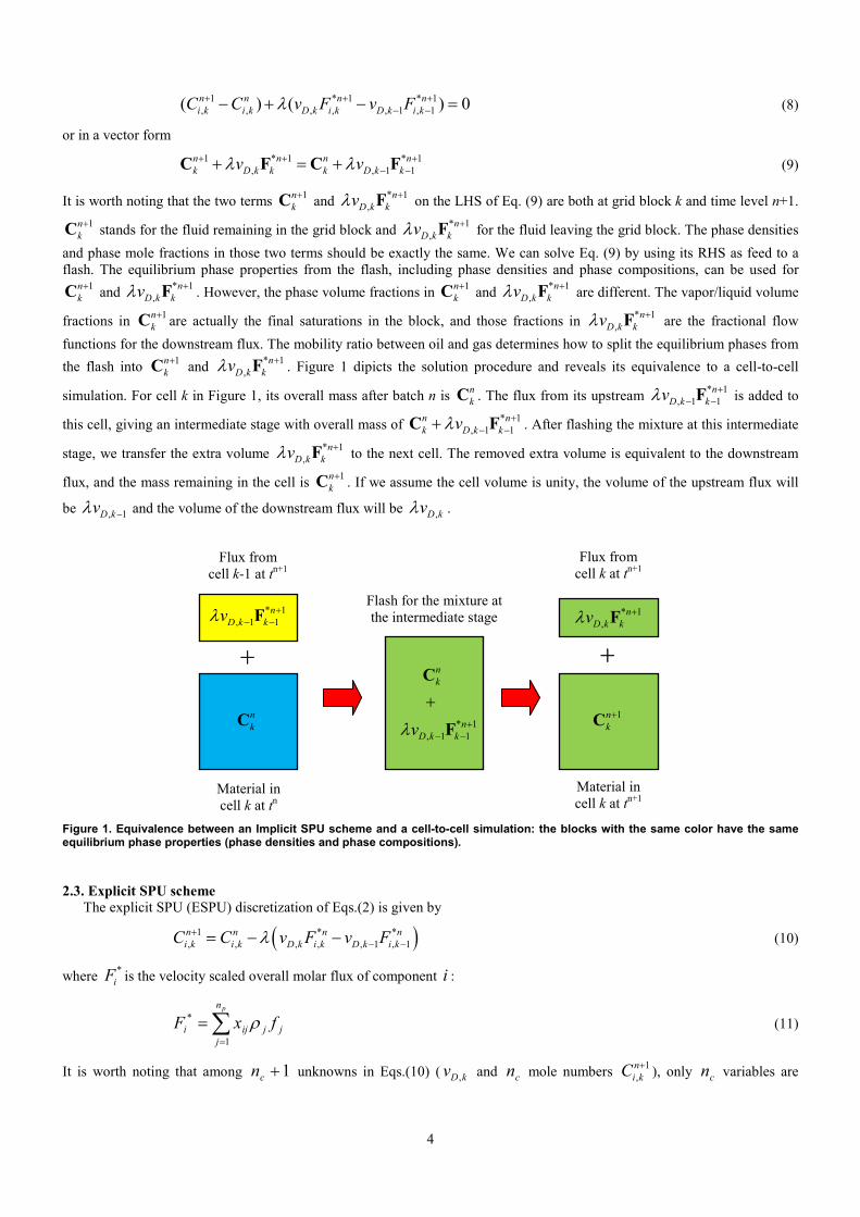
It is worth noting that the two terms 1nk+C and * 1

,n

D k kvλ +F on the LHS of Eq. (9) are both at grid block k and time level n+1. 1n

k+C stands for the fluid remaining in the grid block and * 1

,n

D k kvλ +F for the fluid leaving the grid block. The phase densities and phase mole fractions in those two terms should be exactly the same. We can solve Eq. (9) by using its RHS as feed to a flash. The equilibrium phase properties from the flash, including phase densities and phase compositions, can be used for

1nk+C and * 1

,n

D k kvλ +F . However, the phase volume fractions in 1nk+C and * 1

,n

D k kvλ +F are different. The vapor/liquid volume

fractions in 1nk+C are actually the final saturations in the block, and those fractions in * 1

,n

D k kvλ +F are the fractional flow functions for the downstream flux. The mobility ratio between oil and gas determines how to split the equilibrium phases from the flash into 1n

k+C and * 1

,n

D k kvλ +F . Figure 1 dipicts the solution procedure and reveals its equivalence to a cell-to-cell

simulation. For cell k in Figure 1, its overall mass after batch n is nkC . The flux from its upstream * 1

, 1 1n

D k kvλ +− −F is added to

this cell, giving an intermediate stage with overall mass of * 1, 1 1

n nk D k kvλ +

− −+C F . After flashing the mixture at this intermediate

stage, we transfer the extra volume * 1,

nD k kvλ +F to the next cell. The removed extra volume is equivalent to the downstream

flux, and the mass remaining in the cell is 1nk+C . If we assume the cell volume is unity, the volume of the upstream flux will

be , 1D kvλ − and the volume of the downstream flux will be ,D kvλ .

Figure 1. Equivalence between an Implicit SPU scheme and a cell-to-cell simulation: the blocks with the same color have the same equilibrium phase properties (phase densities and phase compositions). 2.3. Explicit SPU scheme

The explicit SPU (ESPU) discretization of Eqs.(2) is given by

( )1 * *, , , , , 1 , 1n n n ni k i k D k i k D k i kC C v F v Fλ+

− −= − − (10)

where *iF is the velocity scaled overall molar flux of component i :

∑=

=pn

jjjiji fxF

1

* ρ (11)

It is worth noting that among 1+cn unknowns in Eqs.(10) ( kDv , and cn mole numbers 1,ni kC + ), only cn variables are

Material in cell k at tn+1

Flux from cell k at tn+1

Flux from cell k-1 at tn+1

Flash for the mixture at the intermediate stage

Material in cell k at tn

* 1,

nD k kvλ +F

* 1, 1 1

nk

nD k kvλ +

− −

+C

FnkC 1n

k+C

* 1, 1 1

nD k kvλ +

− −F

＋ ＋

5

independent, and kDv , is dependent on 1nk+C . This complicates the solution procedure slightly since there are unknowns on

both sides of the equations. Dindoruk (1992) presents a solution procedure for the ESPU scheme, which has the innermost loop for kDv , . Appendix A reviews the procedure in brief.

Ahamdi and Johns (2008) proposed a multicell algorithm different from the other multicell ones in the literature. It is interesting to notice that their procedure shows some similarity to an explicit SPU FD scheme. The solution procedure starts with just one upstream cell filled with injection gas and one downstream cell filled with initial oil. The two cells are mixed in a certain ratio in the first contact, and the overall mixture is flashed. In the second contact, the equilibrium liquid and gas phases from the first (negative) flash are brought into contact with a newly added cell of injection gas in the upstream and a newly added cell of initial oil in the downstream, respectively. The two resulting mixtures are flashed and give two sets of equilibrium phases. The third contact consists of three mixings: newly added gas with the equilibrium oil in the upstream cell, the equilibrium gas from the upstream cell with the equilibrium oil in the downstream cell, and the equilibrium gas in the downstream cell with newly added oil. The procedure repeats itself by adding injection gas in the upstream and initial oil in the downstream, and the number of flashes increases by one after each contact. This procedure, illustrated in Figure 1 of Ahmadi and Johns (2008), can be compared to an explicit SPU scheme. We can interpret the newly added cell filled with injection gas as the flux from the injector at tn, and the newly added cell filled with initial oil as the downstream cell at tn which is to be updated. For the equilibrium gas and liquid phases from a cell in the middle, we can interpret the former as the flux to the next adjacent cell at tn, and the latter as the content left in the cell at tn. The solution procedure resembles an explicit SPU FD scheme except that the way to determine flux is different in their procedure. 2.4. Higer order explicit method with TVD limitation

1-D gas injection simulation can suffer from severe numerical dispersion for certain systems. We can use a a larger number of grid blocks to achieve a desired accuracy. The maximum grid number, however, is limited by simulation time since the overall time increases with the square of the grid number. Another way to achieve a higher accuracy is to use higher order methods. Higher order methods can lead to spurious oscillation when applied to hyperbolic type gas injection equations. One approach to remove this instability in higher resolution methods is to introduce flux limiters. Using total variation diminishing (TVD) schemes is one of the most prevailing flux limiting methods used for higher order finite difference simulations. Applications of the TVD schemes in black oil type simulations can be found in the works by Rubin and Blunt (1991), Datta Gupta et al. (1991), Rubin and Edwards (1993), and Peddibholta et al. (1997). Thiele et al. (1997) applied a TVD scheme with the van Leer limiter to the 1-D compositional simulations along the streamlines in their 3-D compositional streamline simulations. A different way to construct the flux was proposed by Thiele and Edwards (2001) and the resulting scheme has the nature of a Godunov formulation. Mallison et al. (2005) made an in-depth investigation on the higher-order upwind schemes for two-phase, multicomponent flow, and they suggested using the essentially nonoscillatory (ENO) schemes for such simulations. Here, we use the formulation similar to those of Thiele et al. (1997). A second order scheme with TVD limitation can be formulated as follows:

( )1 * *, , , , 1/2 , 1 , 1/2 n n n n

i k i k D k i k D k i kC C v F v Fλ++ − −= − − (12)

where *, 1/2

ni kF + is calculated as

, 1/2* * * *, 1/2 , , 1 ,( )

2

ni kn n n n

i k i k i k i kF F F F++ +

Φ= + − (13)

with Φ being a TVD limiter. There are several flux limiters that can be chosen (Sweby, 1984; Peddibhotla et al., 1997) and we select the van Leer limiter here:

, 1/2 , 1/2, 1/2

, 1/21

n ni k i kn

i k ni k

r r

r+ +

++

+Φ =

+ (14)

and r is a function of the ratio of adjacent flux difference * *, , 1

, 1/2 * *, 1 ,

n ni k i kn

i k ni k i k

F Fr

F F−

++

−=

− (15)

If Φ is set to zero, the TVD scheme reduces to the explicit SPU scheme. The TVD scheme has almost the same calculation procedure as the explicit SPU scheme. The only difference is that Φ must be calculated for each grid. The computation expenses for two schemes are therefore very similar.

6

3. Determination of MMP by fast slimtube simulations It calls for a comphrensive strategy to improve the computational efficiency for MMP determination by slimtube simulations. The following issues in diverse aspects should be considered:

3.1. Efficient flash algorithm for slimtube simulation

Two-phase isothermal flash is the work-horse in slimtube simulation. Optimization of two-phase isothermal flash for slimtube simulation was discussed by Michelsen (1998). The same optimization approach has been employed here in the slimtube simulation code for MMP determination. The essence of the approach is to use Newton’s method whenever possible. The solution to 1-D gas injection is characterized by a leading single phase oil region, a trailing single phase gas region, and a two-phase gas-oil region in between. In the two-phase region where the previous two-phase results are available, a direct Netwon iteration can always be employed for the new flashes and most of them will converge without a problem. For the flashes that fail to converge or converge to trivial solutions with the direct Newton approach, the conventional flash with stability analysis can be used to safeguard convergence. The unique solution structure of 1-D gas injection also indicates that most single-phase cells will stay in single-phase in the next time step. Therefore, flash calculations in the single-phase regions are only needed in the “safety zones” around the borders between the two-phase region and the single-phase regions. A more rigorous approach is to skip stability analysis in the single phase regions is to use the shadow region method (Rasmussen et al., 2006). For slimtube simulations, our experiences show that the “safety zone” approach is robust enough. Fast flash calculations also require efficient thermodynamic subroutines. For slimtube simulations, a further cut in calculation time can be made by combining the evaluation of thermodynamic properties for the two phases into a single evaluation of the quantities of interest. More details on implementing an efficient two-phase isothermal flash in slimtube simulations can be found in Michelsen (1998).

3.2. Tie-line distance based approximation (TDBA)

The tie-line distance based approximation (TDBA) method, a recently proposed approximation method for flash calculations (Belkadi et al., 2011), is employed here to further reduce the time used in flash calculations. The method is based on the fact that the results from a previous rigorous flash in a grid block could be a good approximation to the new flash in the same block. The distance between the new feed composition and the tie-line from the previous flash, named the tie-line distance, is used as a measure to judge whether to make the approximation or not. If the new feed composition is close enough to the previous flash in terms of the tie-line distance, the previous results will be used either directly or with some adjustment. The tie-line distance d from a feed z to a previous tie-line characterized by equilibrium compositions x and y is given by

( )( )( )22 min 1i i ii

d e z y xβ β= = − + −∑ (16)

where the error e is equal to d2. The vapor fraction β corresponding to the minimum distance is given by

( ) ( )( ) ( )

T

Tβ − −=

− −z x y xy x y x

(17)

Although β is a result of minimization, it can be calculated directly. The original TDBA uses two levels of tolerances. The old flash results will be accepted without any change if the error is less than the smaller tolerance; a new flash is performed if the error is greater than the larger tolerance; and adjustment of the old flash results is needed if the error falls in between the two tolerances. Here, we keep just one level tolerance by removing the smaller one. The flash is proceeded in two different ways depending on the magnitude of e:

• if e > ε, we do new flash; • if e ≤ ε, we use old results but adjustment is needed;

The adjustment can be made in two ways. The first one is to solve the Rachford-Rice equation with the old K-values; the second one is to adjust the material balance using the vapor split factors defined by

( )1i

ii i old

yy x

βθβ β

= + − (18)

The new vapor and liquid flows are calculated as

,i i new iv z θ= ( ), 1i i new il z θ= − (19)

The two options are named TDBA1 and TDBA2, respectively. Both TDBA1 and TDBA2 will preserve material balances in their adjustment.

7

3.3. Extrapolation to RF∞ with a single simulation run Determination of MMP using the recovery-pressure plot needs the oil recovery at 1.2 PVI. We use the C7+ recovery in this

study as the oil recovery. It is well known that FD simulation with a finite number of grid blocks will have numerical dispersion and the dispersion will decrease with increasing number of grid blocks. In the extreme situation of infinite number of grid blocks, the recovery RF∞ is supposed to be dispersion free. To obtain such a RF∞ from a direct simulation run is obviously impossible. A practical way to estimate RF∞ is to extrapolate the recoveries at different numbers of grid blocks (N) to N=∞. Stalkup found that extrapolation using the recovery versus 1/N0.5 gave nearly straight lines. Høier and Whitson (2001) and Jaubert et al. (1998a) also used 1/N0.5 in their extrapolation. Extrapolation seems to require the same number of simulation runs as those recovery points used in the extrapolation. This is actually not necessary since a simulation run with N grid blocks provides essentially the simulation results for any M grid blocks if M is smaller than N. For example, to get the recovery at 1.2 PVI for M grid blocks, we only need to calculate the recovery for the first M grid blocks at 1.2M/N PVI. Therefore, we can get a series of recoveries, e.g., at N=100, 200, 300, 400, and 500, for extrapolation through a single simulation run. Another issue worth noting is that the recovery versus 1/N0.5 is not always a straight line, which was also observed by Høier and Whitson (2001). The curvature can be quite large for systems with large numerical dispersion, especially when it approaches the MMP. To account for the curvature, a second degree polynomial has been used here in the recovery fitting. The fitting procedure is made adaptive since not all the recovery points are equally important to the final trend to 1/N0.5=0. The recovery points at lower N values may affect the fitting for the recovery points at higher N values. In many situations, an extremum may form between the smallest 1/N0.5 and 1/N0.5=0. In that case, the recovery points will be removed one by one from the smallest N. A new regression is made after each removal until such extremum disappears.

3.4. Selection of numerical schemes

Three different numerical schemes are investigated here, namely, ESPU, ISPU, and TVD. If the same Δτ/Δξ is used, three schemes will give similar simulation time. Without the NVC assumption, ISPU is usually a little faster than ESPU or TVD since both ESPU and TVD need to include isothermal flash in their innermost loops. On the other hand, ESPU and TVD also lead to less dispersed results with shaper fronts and longer constant K-values regions, which help to reduce the time for flash calculations since more cells tend to have similar results to the previous ones. Our experiences show that ESPU and TVD are around 10-20% slower than ISPU at the same Δτ/Δξ for simulations without the NVC assumption. With the NVC assumption, there is no need to iterate over the dimensionless velocity vD in ESPU and TVD, and the simulation times for three schemes are very similar. However, as an implicit scheme, ISPU can use much larger Δτ/Δξ than ESPU or TVD. For ESPU and TVD, the maximum stable time step can be calculated by

max( )D i

CFLv

ξτλ∆

∆ =⋅

(20)

where CFL is the Courant-Friedrichs-Lewy number (1 for ESPU and 0.5 for TVD) and (vD·λi)max is the maximum propagation speed (Mallison et al., 2005). To calculate the largest eigenvalue for all the compositions along the slimtube is not practical. One can make a rough estimate of (vD·λi)max and use a constant Δτ before the simulation. Here, we use a different approach by calculating Δτ adaptively during the simulation. For 1-D gas injection simulation with a uniform initial condiiton, the leading front can be readily located and its propagation speed, vmax, can be updated dynamically. The stable time step is estimated by

max

a CFLvξτ ∆

∆ = ⋅ (21)

where a is an empirical parameter to address the difference between vmax and the actual fastest propagation speed which needs to account for the maximum eigenvalue for all the compositions. Our numerical tests show that a =0.5 provides a buffer large enough for stable simulations. Even with the adaptive time stepping, ESPU or TVD will have a maximum time step much smaller than ISPU. Therefore, if the grid number is the same for three schemes, we can obviously get the fastest results from ISPU.

However, some gas injection systems can suffer from severe numerical dispersion which can not be completely removed by recovery extrapolation. To overcome the problem, we can either perform simulation with more grid blocks or resort to a higher order FD scheme without increasing the grid number. The choice has to be made between a simulation using ISPU with more grid blocks and larger time steps and a simulation using TVD with the same grid number but smaller time steps. There is no obvious answer to the question. In principle, the overall simulation time is proportional not to N, but to N2. It seems that TVD is more suitable to systems with severe numerical dispersion. 3.5. Strategy for searching MMP

To determine MMP from the break point in the recovery-pressure plot, we can select a series of pressures to run slimtube simulations. The simulation runs above the MMP always give RF∞ equal to or higher than 100% (due to extrapolation, RF∞ can be higher than 100%). Those runs are not helpful to MMP determination and should be avoided if possible. A MMP search strategy is suggested as follows:

8

(1) The first pressure P1 is selected as a pressure just above the saturation pressure (e.g., rounded to 0 or 5 atm). Perform slimtube simulation at P1. The extrapolated recovery at infinite cells is denoted by RF1. (2) Select the second pressure P2=P1+ΔP, where ΔP can be set to 50 atm. Perform slimtube simulation at P2. The extrapolated recovery at infinite cells is denoted by RF2. (3) If RF2 is higher than 100%, reduce ΔP by half and go to step 2. (4) Select P3=P2+ΔP and calculate the expected recovery at P3 by linear extrapolation based on RF1 and RF2. If the expected recovery is higher than 100%, set P3=(P1+P2)/2. Peform slimtube simulation at P3 and the recovery is denoted by RF3. (5) Fit the recoveries RF1, RF2, and RF3 using an exponential function

2exp( )RF a bP cP= + + (22)

Extrapolate to 100% recovery to get the first MMP (1)MMPP .

(6) Select the new pressure as the mid point of the current MMP and the highest pressure that gives a recovery lower than 100%. Perform slimtube simulation at this pressure. (7) Fit all the recoveries smaller than 100% with Eq. (22) and calculate the new MMP. (8) Compare the new MMP with the previous one. If the deviation is larger than a tolerance (1 atm here), continue to step 6. Otherwise, stop the iteration and output the MMP.

3.6. Parallel computation

We can apply parallel computation to further speed up slimtube simulation. Parallel computation is commonly used for large scale and complex simulations. It demands parallel computers which used to be hardly accessible or afforadable for simple simulation tasks. Nowadays, advance in manufacturing technology has made multi-core processors readily available, and one can easily realize parallel computation of slimtube simulation tasks on a personal computer. We have used OpenMP (Open Multi-Processing) to parallelize our Fortan code for slimtube simulation. OpenMP is an Application Program Interface (API) that supports multi-platform shared-memory parallel programming in C/C++ and Fortran. It is supported by different compilers, including the Intel Fortran Compiler used here. Parallel computation of slimtube simulations can be realized in different ways. The most straightforward way is to parallelize the simulations at different pressures since the simulations at different pressures are completely independent. This parallelization is easy to implement provided that one knows what pressures to calculate in advance. In the search for MMP where simulation is made essentially at one pressure after another, this parallelization approach is not appropriate. A more general way to realize parallelization is to parallelize the most time consuming flash calculation, which are called repeatedly in slimtube simulation. How to implement parallelization depends on what numerical scheme is used and whether the NVC assumption is employed. The simplest situation is that both an explicit scheme (including the explicit scheme with TVD) and the NVC assumption are used. Under such a situation, the calculation at time level tn+1 depends only on the results at time level tn. Provided that the results are already available at tn, we can arbitrarily select a cell at tn+1, calculate its overall composition from the fluxes at tn, and perform a flash. Since the calculation for a cell is completely independent from the properties of the other cells at the same time level, we can parallelize the calculations for all the cells, and even perform the calculations in any arbitrary order. The situation is a bit more complicated if an implicit scheme or the NVC assumption is not used. Figure 1(a) shows a typical ISPU scheme, where the cell properties at xk and tn+1 is determined by the cell properties at xk and tn+1 and the flux from the cell xk-1 and tn+1. For a sequential calculation, with all the cells already calculated at tn, the calculation at tn+1 always starts at the injector and propagates to the producer. To parallelize such a calculation, we can use the approach illustrated in Figure 1(b), where L batches or simulation at L time levels can be performed simultaneously (L=5 in Figure 1(b)). The calculation has such a structure that the the cell to be calculated at tn+1 is always one cell ahead of the cell to be calculated at tn+2 so that the cell to be calculated at a higher time level can always get the required information from the lower adjacent time level. The parallelization is implemented for all the red dots in the L batches. It should be noted that L can be larger than the maximum number of threads available for the machine. Actually, it is usually helpful to use a larger L to counteract the adverse effect of different workload in the flashes in the L batches. A similar approach can be applied to the ESPU scheme or the TVD scheme without NVC assumptions. In the case that there is no NVC assumption, although the scaled flux F* is taken from the previous time level, the dimensionless velocity vD is always treated implicitly (i.e., from the current time level). Therfore, parallelization of these “explicit” schemes requires a strategy similar to that for the implicit scheme. Parallelization of the ESPU scheme without NVC can take exactly the same propagration style as depicted in Figure 1(b), while parallelization of the TVD scheme without NVC requires a slight modification since calculation of the current cell depends on the information from the downstream cell at the previous time level as well. The modification only requires that the cell to be calculated at tn+1 is two cells ahead of the cell at tn.

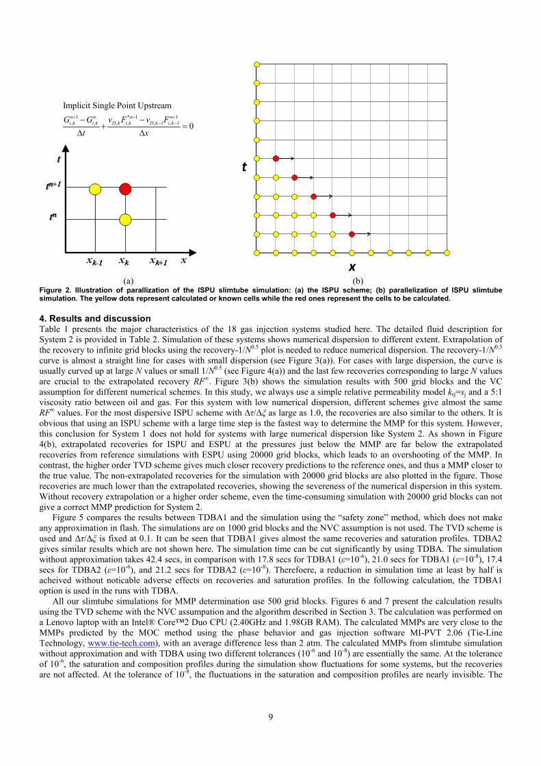
9

t

x (a) (b)

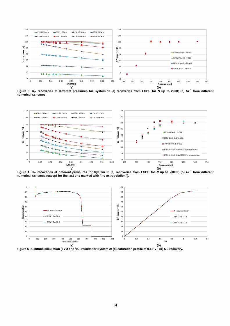
Figure 2. Illustration of parallization of the ISPU slimtube simulation: (a) the ISPU scheme; (b) parallelization of ISPU slimtube simulation. The yellow dots represent calculated or known cells while the red ones represent the cells to be calculated. 4. Results and discussion Table 1 presents the major characteristics of the 18 gas injection systems studied here. The detailed fluid description for System 2 is provided in Table 2. Simulation of these systems shows numerical dispersion to different extent. Extrapolation of the recovery to infinite grid blocks using the recovery-1/N0.5 plot is needed to reduce numerical dispersion. The recovery-1/N0.5 curve is almost a straight line for cases with small dispersion (see Figure 3(a)). For cases with large dispersion, the curve is usually curved up at large N values or small 1/N0.5 (see Figure 4(a)) and the last few recoveries corresponding to large N values are crucial to the extrapolated recovery RF∞. Figure 3(b) shows the simulation results with 500 grid blocks and the VC assumption for different numerical schemes. In this study, we always use a simple relative permeability model krj=sj and a 5:1 viscosity ratio between oil and gas. For this system with low numerical dispersion, different schemes give almost the same RF∞ values. For the most dispersive ISPU scheme with Δτ/Δξ as large as 1.0, the recoveries are also similar to the others. It is obvious that using an ISPU scheme with a large time step is the fastest way to determine the MMP for this system. However, this conclusion for System 1 does not hold for systems with large numerical dispersion like System 2. As shown in Figure 4(b), extrapolated recoveries for ISPU and ESPU at the pressures just below the MMP are far below the extrapolated recoveries from reference simulations with ESPU using 20000 grid blocks, which leads to an overshooting of the MMP. In contrast, the higher order TVD scheme gives much closer recovery predictions to the reference ones, and thus a MMP closer to the true value. The non-extrapolated recoveries for the simulation with 20000 grid blocks are also plotted in the figure. Those recoveries are much lower than the extrapolated recoveries, showing the severeness of the numerical dispersion in this system. Without recovery extrapolation or a higher order scheme, even the time-consuming simulation with 20000 grid blocks can not give a correct MMP prediction for System 2.

Figure 5 compares the results between TDBA1 and the simulation using the “safety zone” method, which does not make any approximation in flash. The simulations are on 1000 grid blocks and the NVC assumption is not used. The TVD scheme is used and Δτ/Δξ is fixed at 0.1. It can be seen that TDBA1 gives almost the same recoveries and saturation profiles. TDBA2 gives similar results which are not shown here. The simulation time can be cut significantly by using TDBA. The simulation without approximation takes 42.4 secs, in comparison with 17.8 secs for TDBA1 (ε=10-6), 21.0 secs for TDBA1 (ε=10-8), 17.4 secs for TDBA2 (ε=10-6), and 21.2 secs for TDBA2 (ε=10-8). Therefoere, a reduction in simulation time at least by half is acheived without noticable adverse effects on recoveries and saturation profiles. In the following calculation, the TDBA1 option is used in the runs with TDBA.

All our slimtube simulations for MMP determination use 500 grid blocks. Figures 6 and 7 present the calculation results using the TVD scheme with the NVC assumpation and the algorithm described in Section 3. The calculation was performed on a Lenovo laptop with an Intel® Core™2 Duo CPU (2.40GHz and 1.98GB RAM). The calculated MMPs are very close to the MMPs predicted by the MOC method using the phase behavior and gas injection software MI-PVT 2.06 (Tie-Line Technology, www.tie-tech.com), with an average difference less than 2 atm. The calculated MMPs from slimtube simulation without approximation and with TDBA using two different tolerances (10-6 and 10-8) are essentially the same. At the tolerance of 10-6, the saturation and composition profiles during the simulation show fluctuations for some systems, but the recoveries are not affected. At the tolerance of 10-8, the fluctuations in the saturation and composition profiles are nearly invisible. The

1 * 1 1, , , , , 1 , 1

Implicit Single Point Upstream

0n n n ni k i k D k i k D k i kG G v F v F

t x

+ + +− −− −

+ =∆ ∆

10

simulation time, however, can be greatly reduced by using TDBA (Figure 7). On average, the MMP search needs simulation runs at 5 pressures. The average simulation time is 33 secs if there is no approximation in flash. It reduces to 18 secs for TDBA with ε=10-8, and 13 secs for TDBA with ε=10-6, indicating that TDBA can cut the MMP calculation time by half. We have also tried MMP determination using ESPU and ISPU, both with TDBA. Using ESPU increases dispersion and does not relax the time step very much. ISPU allows much larger time steps and we have tried Δτ/Δξ = 0.5 and 1.0. Their calculation results are compared with the TVD results in Figure 8. Due to higher dispersions in these schemes, the predicted MMPs are mostly higher than those from the MOC method. There are several cases that ESPU and ISPU give results close to the MOC ones but for System 2, ESPU and ISPU give unacceptable large over-predictions for MMP. The average simulation times for ESPU (ε=10-8), ISPU (ε=10-8 and Δτ/Δξ = 0.5), and ISPU (ε=10-8 and Δτ/Δξ = 1.0) are 15, 12, and 8 secs. The simulation times for ISPU with larger time steps are shorter than that for TVD. However, a significant part of time will be used in the overhead other than flash calculations. The overall simulation is not reduced proportionally with the time step. It seems more adequate to use a low dispersed TVD scheme than a little faster but high dispersed ISPU scheme for the systems studied here.

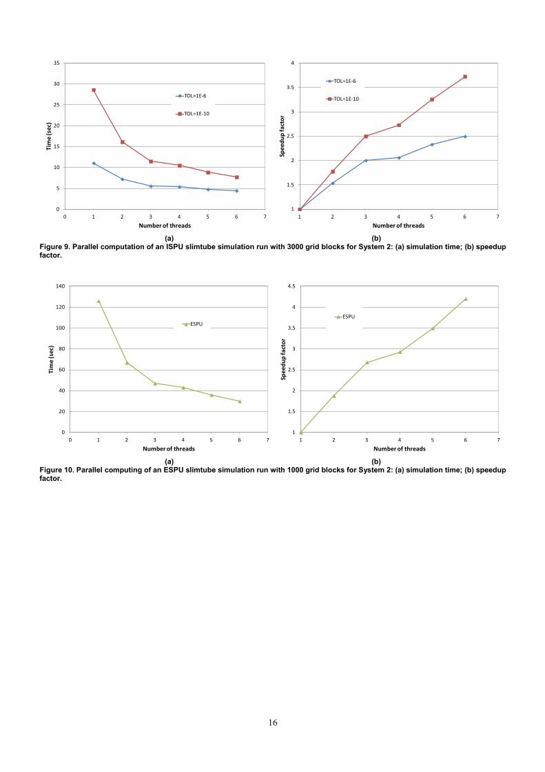
Finally, we illustrate the potential of parallelization using three slimtube simulation tests for System 2. All the tests were made on a personal computer with an AMD Phenom II X6 model 1035T processor (2.6 Ghz, and 3.1 GHz in turbo mode with maximum three cores being active). The first test is on parallelization of simulation runs at different pressures. For simulation at six pressures (300, 320, 340, 360, 380, and 400 atm), it takes 80 secs without parallel computation and 16.8 secs with parallel computation. If we consider that a single core always runs faster, the scaling is almost perfect. The second test is on parallelization of an ISPU slimtube simulation using the approach described in Section 3.6. For 3000 grid blocks and 6000 time steps, the times needed for a simulation run at 300 atm with TDBA (ε=10-6 and 10-10) are shown in Figure 9, together with the speedup factors. In the parallel computation, the number of loops L is set to 60. The simulation time decreases with the number of threads used but not in a simple inversely proportional relation, especially for the run with ε=10-6. One reason for this is that the overhead other than flash calculation is more significant when the simulation time is short. For the longer simulation with ε=10-10, the speedup performance is better. Another reason is that the turbo mode is only available for three cores, and the decrease in simulation time will be affected if the number of threads is larger than three. The third test is on parallelization of an ESPU slimtube simulation with the NVC assumption, where all the flash calculations at the same time level can be computed in a parallel mode. For a simulation run at 300 atm with 1000 grid blocks and the adaptive time stepping, the results using flash with full stability analysis aree shown in Figure 10. The scalability is satisfactory if we consider that the turbo mode is only available for maximum three cores. By comparing the three tests, it seems that direct parallelization of simulation runs at different pressures is the most efficient since the overhead in running OpenMP is larger for parallelization of flash calculations. However, the former requires more memory and is less flexible in a sequential MMP search algorithm.

5. Conclusions Numerical simulation of the slimtube experiment provides a reliable way to calculate MMP since the calculation procedure resembles the experimental MMP determination procedure. Different variations of the slimtube simulation, including multicell simulations and 1-D FD simulations, are based on the same mathematical formulation of 1-D gas injection. We have investigated how to speed up MMP determination based on slimtube simulations. Development of such a fast algorithm needs a comphrensive effort in many aspects. A fast flash subroutine with an efficient thermodynamic package forms the basis of the algorithm. The unique structure of the 1-D gas injection solution can be used to skip most stability analysis in the single phase regions and to apply Newton’s method directly in flash calculations in the two-phase region. Extrapolation to recovery at infinite cells is essential to reduce numerical dispersion and can be performed with the information from a single simulation run. Higher order methods, such as the ESPU scheme with TVD, can be employed to reduce the number of grid blocks needed. An adaptive time stepping is recommended if an explicit scheme is used. TDBA can be applied to get essentially the same recoveries at 50% or even shorter simulation time. Finally, a MMP search strategy is crucial to reduce the number of simulation runs at different pressures. We also point out that the advance in computer hardware, namely multicore CPU, could be readily utilized for parallel computation in slimtube simulation. Our tests using 18 multicomponent gas injection systems have shown that our code developed using the aforementioned principles give the MMP results similar to those from the MOC method. The average MMP calculation time for the TVD scheme with TDBA is around 15 secs for those 12~15 components systems on a common laptop (without parallelization). The algorithm presented here can be further refined in terms of, for instance, the number of grid blocks, selection of numerical schemes, and details in the searching strategy, which should be based on a large scale MMP calculation tests. Nevertheless, the algorithm has provided an efficient MMP calculation approach complementary to the fast MOC method. The additional information provided by MMP determination using slimtube simulation, such as saturation/composition profiles and oil recoveries, are also beneficial to understanding the real gas injection process.

Acknowledgements This study has been carried out under the project “ADORE—Advanced Oil Recovery Methods” funded by the Danish Council for Technology and Production Sciences, Maersk Oil, and DONG Energy.

11

Appendix A. Solution procedure for the ESPU scheme The solution procedure consists of three-level loops, the outermost one for time, the middle one for space, and the innermost one for velocity kDv , . The solution of kDv , must satisfy the overall mass balance equation:

1 * *, , , , , 1 , 1

1 1 1 1

c c c cn n n nn n n ni k i k D k i k D k i k

i i i iC C v F v Fλ+

− −= = = =

= − −

∑ ∑ ∑ ∑ (23)

which is obtained by summing Eqs. (10) over all the components. Since 1,

1

cnni k

iC +

=∑ represents the overall density at tn+1, it

should be equal to the overall density calculated from the phase equilibrium: 1

1

v l

β βρρ ρ

− −

= +

(24)

Dindoruk suggests using the overall density ρ instead of vd as iterative variable since it makes the procedure more robust. The final procedure for a grid block k is as follows:

1. Use the overall density from the previous time step as initial estimate for ρ;

2. Calculate ,1

cnni k

iC

=∑ , *

,1

cnn

i ki

F=∑ , and *

, 11

cnn

i ki

F −=∑ at time level n;

3. Calculate vD,k by rearranging Eq. (23):

* *, , , 1 , 1 ,

1 1 1( ) / ( )

c c cn n nn n n

D k i k D k i k i ki i i

v C v F Fρ λ λ− −= = =

= − +∑ ∑ ∑ (25)

4. Calculate 1,ni kC + by Eqs.(10) using the newly calculated vD,k;

5. Flash the mixture in the block with composition 1,ni kC + (normalization needed);

6. Calculate the new density ρ by Eq. (24) and compare it with 1,

1

cnni k

iC +

=∑ . If the relative error smaller than the tolerance

(10-3~10-4), stop iteration; otherwise, go to step 3. In our code, we use a secant method for ρ instead of direct substitution. For explicit scheme with TVD, the same procedure can be used. If it is assumed no volume change on mixing (NVC), the procedure can be simplified since kDv , is always equal to 1 and no innermost loop is needed.

References Ahmadi, K., Johns, R., 2008. Multiple Mixing-Cell Method for MMP Calculations. Paper SPE 11823 presented at the 2008 SPE Annual

Technical Conference and Exhibition held in Denver, Colorado, USA, September 21-24, 2008. Belkadi, A., Yan, W., Michelsen, M.L., Stenby, E.H., 2011. Comparison of Two Methods for Speeing up Flash Calculations in

Compositional Simulations. Paper SPE 142132 presented at the SPE Reservoir Simulation Symposium held in The Woodlands, Texas, USA, 21-23 February 201.

Cook, A.B., Walker, C.J., Spencer, G.B., 1969. Realistic K Values of C7+ Hydrocarbon for Calculating Oil Vaporization During Gas Cycle at High Pressures. Journal of Petroleum Technology 21(7): 901-915.

Datta Gupta, A., Lake, L.W., Pope, G.A., Sepehrnoori, K., 1991. High-Resolution Monotonic Schemes For Reservoir Fluid Flow Simulation. In-Situ 15(3): 289-317.

Dindoruk, B., 1992. Analytical Theory of Multiphase Multicomponent Displacement in Porous Media. Ph.D. Thesis, Department of Petroleum Engineering, University of Stanford, California, USA.

Jaubert, J.N. Wolff, L., Neau, E., Avaullee, L., 1998a. A Very Simple Multiple Mixing Cell Calculation to Compute the Minimum Miscibility Pressure Whatever the Displacement Mechanism. Industrial & Engineering Chemistry Research 37 (12): 4854-4859.

Jaubert, J.N., Arras, L., Neau, E., Avaullee, L. 1998b. Properly Defining the Classical Vaporizing and Condensing Mechanisms When a Gas Is Injected into a Crude Oil. Industrial & Engineering Chemistry Research 37 (12): 4860-4869.

Jessen, K. 2000. Effective Algorithms for the Study of Misccible Gas Injections Processes. PhD Thesis, Department of Chemical Engineering, Technical University of Denmark, Copenhagen, Denmark.

Jessen, K., Michelsen, M.L., Stenby, E.H., 1998. Global Approach for Calculation of Minimum Miscibility Pressure. Fluid Phase Equilibria 153 (2): 251-263.

12

Johns, R.T., Orr, F.M., Jr., 1996. Miscible Gas Displacement of Multicomponent Oils, SPE Journal 1(1): 39-50. Høier, L., Whitson, C.H., 2001. Miscibility Variation in Compositionally Grading Reservoirs. SPE Reservoir Evaluation & Engineering

February: 36-43. Mallison, B.T., Gerritsen, M.G., Jessen, K., Orr, F.M., Jr., 2005. High-Order Upwind Schemes for Two-Phase, Multicomponent Flow. SPE

Journal September 297-311. Metcalfe, R.S., Fussell, D.D., Shelton, J.L., 1973. A Multicell Equilibrium Separation Model for the Study of Multiple Contact Miscibility in

Rich-Gas Drives. SPE Journal June: 147-155. Michelsen, M.L., 1998. Speeding up the Two-Phase PT-flash, with Applications for Calculation of Miscibile Displacement. Fluid Phase

Equilibria 143: 1-12. Monroe, W.W., Silva, M.K., Larsen, L.L., Orr, F.M., Jr., 1990. Composition Paths in Four-Component Systems: Effect of Dissolved

Methane on 1D CO2 Flood Performance. SPE Reservoir Eng. 5(3), 423-432. Orr, F. M. 2007. Theory of Gas Injection Processes. Tie-Line Publications, Holte, Denmark. Peddibhotla, S., Datta-Gupta, A., Xue, G., 1997. Multiphase Streamline Modeling in Three Dimensions: Further Generalizations and A Field

Application. Paper SPE 38003 presented at the 1997 SPE Reservoir Simulation Symposium held in Dalia, Texas, 08-11 June 1997. Pedersen, K.S., Fjellerup, J., Thomassen, P., 1986. Studies of Gas Injection Into Oil Reservoirs by a Cell-to-Cell Simulation Model. Paper

SPE 15599 presented at the 61st Annual Technical Conference and Exhibition of the Society of Petroleum Engineering held in New Orleans, LA, October 5-8, 1986.

Rasmussen, C. P., Krejberg, K., Michelsen, M. L., Bjurstrom, K. E. 2006. Increasing the Computational Speed of Flash Calculations with Applications for Compositional, Transient Simulations. SPE Res Eval & Eng 9: 32-38.

Rubin, B., Blunt, M.J., 1991. Higher-Order Implicit Flux Limiting Schemes for Black Oil Simulation. Paper SPE 21222 presented at the 11th SPE Symposium on Reservoir Simulation held in Anaheim, California, February 17-20, 1991.

Stalkup, F.I., 1987. Dispacement Behavior of the Condensing/Vaporizing Gas Drive Process. Paper SPE 16715 presented at the 62nd Annual Technical Conference and Exhibition of the Society of Petroleum Engineers held in Dallas, TX, September 27-30, 1987.

Stalkup, F., 1990. Effect of Gas Enrichment and Numerical Dispersion on Enriched-Gas-Drive Predictions. SPE Reservoir Engineering, November, 647-655.

Stalkup, F.I., Lo, L.L., Dean, R.H., 1990. Sensitivity to Gridding of Miscible flood Predictions Made With Upstream Differenced Simulations. Paper SPE 20178 presented at the SPE/DOE seventh Symposium on Enhanced Oil Recovery held in Tulsa, Oklahoma, April 22-25, 1990.

Sweby, P.K., 1984. High Resolution Schemes Using Flux Limiters for Hyperbolic Conservation Laws. SIAM Journal on Numerical Analysis 21(5) 995-1011.

Thiele, M.R., Batycky, R.P., Blunt, M.J., 1997. A Streamline-Based 3D Field-Scale Compositional Reservoir Simulator. Paper SPE 38889 presented at the Annual Technical Conference and Exhibition held in San Antonio, TX, October 5-8, 1997.

Thiele, M.R., Edwards, M.G., 2001. Physically Based Higher Order Godunov Schemes for Compositional Simulation. Paper SPE 66403 presented at the SPE Reservoir Simulation Symposium held in Houston, Texas, February 11-14, 2001.

Wang, Y., Orr, F.M., Jr., 1997. Analytical Calculation of Minimum Miscibility Pressure. Fluid Phase Equilibria 137: 101-124. Zhao, G.B., Adidharma, H., Towler, B., Radosz, M., 2006. Using a Multiple-Mixing-Cell Model to Study Minimum Miscibility Pressure

Controlled by Thermodynamic Equilibrium Tie Lines. Ind. Eng. Chem. Res. 45: 7913-7923. Zick, A.A., 1986. A Combined Condensing/Vaporizing Mechanism in the Displacement of Oil by Enriched Gases. Paper SPE 15493

presented at the 61st Annual Technical Conference and Exhibition of Society of Petroleum Engineers held in New Orleans, LA, October 5-8, 1986.

13

Table 1. Overview of the four gas injection systems

System EoS N2/CO2/C1 C2-C6 C7+ nc Tres (K) Pbub (atm) MMP (atm) 1 SRK 24 32 44 15 374.85 98.99 215.93 2 SRK 44 23 33 13 375.00 248.14 315.26 3 PR 25 18 57 12 358.15 97.2 149.7 4 PR 42 16 42 12 358.15 191.14 204.02 5 PR 47 18 35 15 368.15 237.45 519.17 6 PR 47 18 35 15 368.15 237.45 369.32 7 SRK 25 29 46 15 372.05 117.62 245.54 8 SRK 48 23 29 15 387.35 252.16 365.05 9 SRK 58 21 21 15 388.15 316.5 368.33

10 SRK 29 28 43 15 394.25 153.41 260.04 11 SRK 37 29 34 15 383.15 168.14 286.11 12 SRK 37 29 34 15 383.15 168.14 299.65 13 SRK 33 30 37 15 393.15 154.78 295.85 14 SRK 34 30 36 15 393.15 148.35 277.26 15 SRK 51 22 27 15 394.25 249.69 269.12 16 SRK 48 23 29 15 373.75 245.46 353.56 17 SRK 50 24 26 15 376.45 274.23 304.9 18 SRK 40 20 41 15 377.55 170.64 250.64

Table 2. Fluid description for gas injection system 2

zoil zgas Tc (K) Pc (atm) ω MW (g/mol) kCO2,j

CO2 0.003712 0.8 304.2 72.8 0.225 44.01 0.00 C1 0.437387 0.2 190.6 45.4 0.008 16.04 0.12 C2 0.074353

305.4 48.2 0.098 30.07 0.12

C3 0.062312

369.8 41.9 0.152 44.09 0.12 i-C4 0.010436

408.1 36.0 0.176 58.12 0.12

C4 0.031507

425.2 37.5 0.193 58.12 0.12 i-C5 0.01154

460.4 33.4 0.227 72.15 0.12

C5 0.016557

469.6 33.3 0.251 72.15 0.12 C6 0.022477

507.4 29.3 0.296 86.17 0.12

C7 0.034417

529.5 32.3 0.4591 100.20 0.10 C8 0.040839

547.1 30.4 0.4854 114.23 0.10

C9 0.025386

568.1 27.4 0.5228 128.25 0.10 C22 0.229078

810.3 15.1 1.0315 310.60 0.10

14

70

75

80

85

90

95

100

105

110

0 0.02 0.04 0.06 0.08 0.1 0.12 0.14 0.16

C7+

reco

very

(%)

1/SQRT(N)

ESPU 120atm ESPU 170atm ESPU 220atm ESPU 250atm

ESPU 300atm ESPU 350atm ESPU 400atm ESPU 500atm

70

75

80

85

90

95

100

105

110

100 150 200 250 300 350 400 450 500 550

C7+

reco

very

(%)

Pressure (atm)

ISPU dt/dx=0.1 N=500

ISPU dt/dx=1.0 N=500

ESPU dt/dx=0.1 N=500

TVD dt/dx=0.1 N=500

(a) (b)

Figure 3. C7+ recoveries at different pressures for System 1: (a) recoveries from ESPU for N up to 2000; (b) RF∞ from different numerical schemes.

75

80

85

90

95

100

105

110

0 0.02 0.04 0.06 0.08 0.1 0.12 0.14 0.16

C7+

reco

very

(%)

1/SQRT(N)

ESPU 250atm ESPU 275atm ESPU 300atm ESPU 325atm

ESPU 350atm ESPU 400atm ESPU 450atm ESPU 500atm

70

75

80

85

90

95

100

105

110

200 250 300 350 400 450 500 550

C7+

reco

very

(%)

Pressure (atm)

ISPU dt/dx=0.1 N=500

ESPU dt/dx=0.1 N=500

TVD dt/dx=0.1 N=500

ESPU dt/dx=0.1 N=20000 (extrapolation)

ESPU dt/dx=0.1 N=20000 (no extrapolation)

(a) (b)

Figure 4. C7+ recoveries at different pressures for System 2: (a) recoveries from ESPU for N up to 20000; (b) RF∞ from different numerical schemes (except for the last one marked with “no extrapolation”).

0

0.1

0.2

0.3

0.4

0.5

0.6

0.7

0.8

0.9

1

0 100 200 300 400 500 600 700 800 900 1000

Gas s

atur

atio

n

Grid block number

No approximation

TDBA1 Tol=1E-6

TDBA1 Tol=1E-8

0

10

20

30

40

50

60

70

80

90

100

0 0.2 0.4 0.6 0.8 1 1.2 1.4

C7+

reco

very

(%)

PVI

No approximation

TDBA1 Tol=1E-6

TDBA1 Tol=1E-8

(a) (b)

Figure 5. Slimtube simulation (TVD and VC) results for System 2: (a) saturation profile at 0.6 PVI; (b) C7+ recovery.

15

0

100

200

300

400

500

600

1 2 3 4 5 6 7 8 9 10 11 12 13 14 15 16 17 18

MM

P (a

tm)

System

MOCNo approximationTDBA Tol=1E-8TDBA Tol=1E-6

-15

-10

-5

0

5

10

15

1 2 3 4 5 6 7 8 9 10 11 12 13 14 15 16 17 18

Devi

atio

n in

MM

P (a

tm)

System

TVD no approximation

TVD TDBA Tol=1E-8

TVD TDBA Tol=1E-6

(a) (b)

Figure 6. MMP calculation results using the TVD scheme: (a) MMP; (b) deviation in MMP.

0

10

20

30

40

50

60

70

1 2 3 4 5 6 7 8 9 10 11 12 13 14 15 16 17 18

Tim

e (s

ec)

System

Reference

TDBA Tol=1E-8

TDBA Tol=1E-6

Figure 7. Simulation time for MMP calculation by slimtube simulation using TVD.

-20

-10

0

10

20

30

40

50

60

70

80

90

1 2 3 4 5 6 7 8 9 10 11 12 13 14 15 16 17 18

Devi

atio

n in

MM

P (a

tm)

System

TVD TDBA Tol=1E-8

ESPU TDBA Tol=1E-8

ISPU TDBA Tol=1E-8 dt/dx=0.5

ISPU TDBA Tol=1E-8 dt/dx=1.0

Figure 8. Deviations in MMP between the slimtube results and the MOC results

16

0

5

10

15

20

25

30

35

0 1 2 3 4 5 6 7

Tim

e (s

ec)

Number of threads

TOL=1E-6

TOL=1E-10

1

1.5

2

2.5

3

3.5

4

1 2 3 4 5 6 7

Spee

dup

fact

or

Number of threads

TOL=1E-6

TOL=1E-10

(a) (b)

Figure 9. Parallel computation of an ISPU slimtube simulation run with 3000 grid blocks for System 2: (a) simulation time; (b) speedup factor.

0

20

40

60

80

100

120

140

0 1 2 3 4 5 6 7

Tim

e (s

ec)

Number of threads

ESPU

1

1.5

2

2.5

3

3.5

4

4.5

1 2 3 4 5 6 7

Spee

dup

fact

or

Number of threads

ESPU

(a) (b)

Figure 10. Parallel computing of an ESPU slimtube simulation run with 1000 grid blocks for System 2: (a) simulation time; (b) speedup factor.