Vol.:(0123456789)1 3

Journal of Petroleum Exploration and Production Technology (2019) 9:889–897 https://doi.org/10.1007/s13202-018-0558-9

ORIGINAL PAPER - EXPLORATION GEOPHYSICS

Calculation of anisotropy permeability from 3D tomographic images using renormalization group approaches and lattice Boltzmann method

Z. Irayani1 · U. Fauzi2 · S. Viridi3 · F. D. E. Latief2

Received: 28 February 2018 / Accepted: 5 October 2018 / Published online: 11 October 2018 © The Author(s) 2018

AbstractCalculation of permeability from 3D tomographic rock images was performed by combining renormalization group approaches (RGA) and lattice Boltzmann method (LBM). Images of sandstone rock samples (i.e., Fontainebleau, Berea, and Sumatera sandstones) with block size of 2563 voxels were used in this study. LBM was applied to calculate permeability of each smallest block (i.e., 64 and 128 voxels) as sub-blocks of the larger block (2563 voxels). The calculated permeability will form analogue to hydraulic conductance networks. RGA were then applied to the networks for all three perpendicular directions using several RGA schemes, i.e., King, Karim–Krabbenhoft, Green–Paterson, and their combinations. It was shown that as the number of renormalizations increases, the average permeability decreases. The effective permeability calculated by combining RGA and LBM were lower than permeability of the single largest block. Karim and Krabbenhoft’s scheme produced mostly higher estimation than the others and closest to the true permeability. Degree of anisotropy is influenced by the initial block size prior to RGA scheme.

Keywords Permeability · Lattice Boltzmann Method (LBM) · Renormalization group approach (RGA) · Anisotropy · Micro-CT scan

Introduction

Permeability, which is a measure of the ability of porous medium to transmit fluids, is an important parameter required in many areas, such as reservoir engineering, hydrology, and environmental engineering. Anisotropy of permeability or multi directional permeability calculation is also crucial for understanding the directions of potential permeable fluid migration, for example, in volcanic rocks

(Wright et al. 2006). Measurements of permeability in the laboratory on core samples are usually conducted in one direction while the permeability in the other direction must be obtained by measuring different core plugs (Farquhar-son et al. 2016). Since permeability of rocks varies due to their pore structures heterogeneity and also depends on the direction of the measurements, different core plugs may give different results. It will influence interpretation of reservoirs and result of fluid flow modeling. As an example, the finite-time (short-term) amount of CO2 which can be dissolved in anisotropic sedimentary rocks is much larger than in iso-tropic rocks (De Paoli et al. 2016).

Several techniques have been developed to easily esti-mate the permeability of rocks and its anisotropy (Fauzi 2011; Iscan and Kok 2009; Jin et al. 2004; Kameda and Dvorkin 2004). Digital image processing was used to cal-culate permeability of rocks from two dimensional images obtained from thin sections (Fauzi 2011; Iscan and Kok 2009; Jin et al. 2004; Kameda and Dvorkin 2004). Tech-niques for anisotropic permeability estimation from 3D microtomographic images were also developed by many authors (Aharony et al. 1991; Rama et al. 2011), but it still

* U. Fauzi umarf@fi.itb.ac.id

1 Physics Department, Faculty of Mathematics and Natural Sciences, Jenderal Soedirman University, Purwokerto, Indonesia

2 Earth Physics and Complex System Research Division, Faculty of Mathematics and Natural Sciences, Bandung Institute of Technology, Bandung, Indonesia

3 Nuclear Physics and Biophysics Research Division, Faculty of Mathematics and Natural Sciences, Bandung Institute of Technology, Bandung, Indonesia

890 Journal of Petroleum Exploration and Production Technology (2019) 9:889–897

1 3

needs further investigation. As an alternative, estimation of absolute permeability in three perpendicular direc-tions from a microscopic 3-D image may be conducted by means of LBM. Intensive and time consumption in com-putational processes for large-size samples are, however, becoming issues for this methodology (Liu et al. 2014). Liu et al. (2016) reported that that simulated permeability obtained from LBM after segmentation processes to reduce computing times are 6–9 times higher than the laboratory measurements.

Renormalization group approaches (RGA) are inten-sively applied to calculate permeability and to investi-gate its anisotropy (Green and Paterson 2007; Karim and Krabbenhoft 2010; King 1989). Firstly, RGA was devel-oped and applied to calculate effective permeability of permeability distribution functions (King 1989). It was then applied to evaluate macroscopic permeability of oil reservoir (Green and Paterson 2007) and images of rock-thin sections (Fauzi 2011). Simple analytical approxima-tion was applied to the method of RGA developed previ-ously (Green and Paterson 2007). A new renormalization scheme was introduced and gave more accurate results than existing schemes (Karim and Krabbenhoft 2010). An approximation technique based on Laplace solver and RGA was used to calculate permeability of 3D tomo-graphic rock samples (Khalili et al. 2012).

In this work, simple and less time-consuming techniques are proposed to calculate permeability and its anisotropy from 3D tomographic images. A combination of LBM and RGA was applied to calculate permeability for the three dimensional micro-CT images of three different types of sandstones: Fontainebleau (FO), Berea (BE), and Sumatra (SU). Several renormalization schemes (Green and Pater-son 2007; Karim and Krabbenhoft 2010; King 1989) and the combination of the three methods were applied in this study.

Methodology

Renormalization group approach (RGA)

The renormalization group approach (RGA) is an elegant method which can be easily applied to obtain equivalent fluid permeability (King 1989) from porous media samples. RGA models a permeable block in the sample as a resistor net-work. A block with permeability k has the equivalent resistor between the mid-points of the edges of 1/k. In three-dimen-sional block, a single block is divided into eight cells. Each cell has a permeability of k1, k2, k3, …, k8, respectively. In the horizontal (x) direction, each edge is assigned a pressure Pi and P0. Dead-end branches in the z and y directions were ignored or cut, and were joined with the corresponding pres-sure nodes. The network can be simplified to calculate the effective value using the star–triangle transformation (King 1989). By assuming that the fluid flows from the center of one cell to the center of each adjoining cell, the effective perme-ability can be estimated by averaging the 2D effective perme-ability of four components, i.e., the top and bottom halves of the block (see Fig. 1). The effective permeability of a three-dimensional block (keff 3D) in the x direction is calculated using the following equation (Green and Paterson 2007):

A new scheme method of renormalization was introduced by Karim and Krabbenhoft (2010) and is shown in Fig. 2. It presents the configuration scheme of a block with eight cells, each with a permeability of k1, k2, k3, k4,… k8 . For

(1)

keff 3D

(

k1, k2, k3, k4, k5, k6, k7, k8)

=1

4

[

keff 2D

(

k3, k4, k7, k8)

+ keff 2D

(

k1, k2, k5, k6)

+ keff 2D

(

k1, k3, k5, k7)

+keff 2D

(

k2, k4, k6, k8)]

.

Fig. 1 Schematic illustration of the two-dimensional renormalization blocks used in the approximation of the three-dimensional renormalization (Green and Paterson 2007)

891Journal of Petroleum Exploration and Production Technology (2019) 9:889–897

1 3

the configuration shown in Fig. 2b, the block-permeability is given by the following equation (Karim and Krabbenhoft 2010):

where subscript a and h are arithmetic and harmonic mean, respectively.

For the configuration shown in (Fig. 2c), the permeability is calculated as follows:

The effective permeability in the x direction is the geo-metric mean of both configurations (Karim and Krabbenhoft 2010):

(2)kL,x = �a[�h(k1, k2),�h(k3, k4),�h(k5, k6),�h(k7, k8)],

(3)kU,x = �h[�a(k1, k3, k5, k7),�a(k2, k4, k6, k8)].

(4)keff,x =(

kL,xkU,x)

1

2 =1

2

[(

k1 + k3 + k5 + k7)(

k2 + k4 + k6 + k8)

(

k1 + k2)(

k3 + k4)(

k5 + k6)(

k7 + k8)

]1

2(

J

I

)

1

2

,

The three methods above may also be combined to calcu-late the effective permeability to compare the results.

These four methods, i.e., King, GP, KK, and a combina-tion of King–GP–KK were applied to the uniform and log-normal permeability distribution generated using a random number generator. The values of the uniformed permeability distribution is generated in the range of 1–9 with a mean

I = k1 + k2 + k3 + k4 + k5 + k6 + k7 + k8,

J = k1k2S12 + k3k4S34 + k5k6S56 + k7k8S78,

(5)Sij =(k1 + k2)(k3 + k4)(k5 + k6)(k7 + k8)

ki + kj.

Fig. 2 Schematic illustration of the two-dimensional renormalization blocks used in the approximation of the three-dimensional renormalization (Karim and Krabbenhoft 2010)

a b

Fig. 3 a Distribution of permeability during renormalization processes for log-normal distribution, b comparison of the number of renormaliza-tion to the mean data from the four RGA scheme for log-normal distribution

892 Journal of Petroleum Exploration and Production Technology (2019) 9:889–897

1 3

(µ) of 5, and the log-normal distribution is generated using � = 5 and standard deviation � = 0.5 . The renormalization procedure was performed until a single effective permeabil-ity is obtained.

The probability density function (PDF) of the uniform and log-normal distribution with 87 data are shown in Fig. 3. The renormalization procedure was applied to the data which later produced a plot of PDF.

In case of the uniform distribution, from the first to the last (fourth) renormalization produced a normal distribu-tion. For the log-normal distribution, the first renormaliza-tion forms the log-normal distribution. On the other hand, the second, third and fourth renormalization changed the distribution into a normal distribution. Thus, we can gen-erally observe that the renormalization process causes the distribution to change into a normal distribution.

Figure 3b shows the change in average permeability dur-ing the renormalization processes. As the number of renor-malizations increases, the average permeability decreases. KK’s scheme produced the highest values and GP’s scheme gave the lowest estimation. The King’s and the combined RGA schemes yielded values that fall in between the other techniques.

Lattice Boltzmann method

Lattice Boltzmann method (LBM) is one of the many techniques in fluid flow simulation which has gained a wide acceptance due to its easiness of implementation of boundary conditions and numerical stability in vari-ous conditions with various Reynolds numbers. In this method, fluid is treated as a collection of particles which is represented by a velocity distribution function at each discrete lattice node. The particles collide with each other and the rules governing the collisions are designed such that the time-average motion of the particles is consistent with the Navier–Stokes equations. In LBM, the computa-tion of each node at every time step depends solely on the properties of itself and the neighboring nodes at the previous time step.

Various LB models exist for numerical solutions of vari-ous fluid flow scenarios, where each model has different way of characterizing microscopic movement of the fluid particles. The LB models are usually denoted as DxQy where x and y corresponds to the number of dimensions and number of microscopic velocity directions (ei), respectively. For example, D2Q9 represents a two-dimensional geometry with nine microscopic velocity directions. The following sub chapter will give general picture of the lattice D2Q9 and D3Q19 LB models which were implemented here. These models obey the distributions function (Kutay and Aydilek 2005):

where Feq

i is the equilibrium distribution function, ρ is the

density, u is the macroscopic velocity of the node. The relax-ation time relates to viscosity of fluid (ν) as follows:

The macroscopic properties, density and velocity, of the nodes are calculated using the following relations:

where ρ and u are the macroscopic density and velocity of the fluid at each node of lattice.

Samples

Three types of digitized sandstones [i.e., Fontainebleau (FO), Berea (BE), and Sumatra (SU)] were used as samples in this study. The FO and BE samples were already in the form of digital binary images (available for public, for exam-ple at https ://goo.gl/RRWjf n), whereas the SU sample was a core plug with a diameter of 1.5 in. A subsample of SU with a dimension of 4 × 9 × 10 mm3 was taken from the core plug to be digitized. Digital images of SU were obtained using a SkyScan 1173 micro-CT scanner. The scanning was per-formed using X-ray energy of 130 kV and current of 60 µA filtered by a 0.25 mm brass filter. The projection image of the sample is acquired by a flat-panel detector with dimen-sion of 2240 × 2240 pixels and exposure time of 1250 ms. The sample stage is rotating 180° at a rotation step of 0.2°. The scanning process took 102 min which produced 1200 raw projection images (16 bit TIFF images) in a total of ~ 11.4 GB size of files. Measured porosity and permeability of the core samples are 14.84% and 1300 mD, 16.00% and 1100 mD, 24.52% and 1865 mD for FO, BE, and SU respec-tively (Dong 2008; Latief et al. 2010).

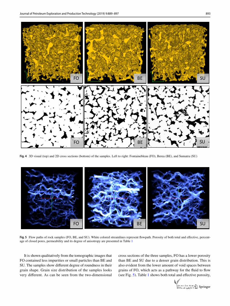
Subsequent to the scanning and reconstruction process, segmentation by means of global-threshold method (Otsu method) was applied to the samples to produce a distin-guished pore-void phase in the form of binary image. Fig-ure 4 shows the three dimensional view as well as the two dimensional cross sections of the samples to observe the pore structures of each sample. Figure 5 provides velocity profiles generated by LBM method for sample image size of 2563.

(6)Feq

i= wa�

[

1 +��⋅ �

c2s

+

(

��⋅ �

)2

2c4s

−� ⋅ �

2c2s

]

,

(7)� = c2s

(

� −1

2

)

.

(8)� =

Q�

i=1

Fi, � =

Q∑

i=1

Fi

�,

893Journal of Petroleum Exploration and Production Technology (2019) 9:889–897

1 3

It is shown qualitatively from the tomographic images that FO contained less impurities or small particles than BE and SU. The samples show different degree of roundness in their grain shape. Grain size distribution of the samples looks very different. As can be seen from the two-dimensional

cross sections of the three samples, FO has a lower porosity than BE and SU due to a denser grain distribution. This is also evident from the lower amount of void spaces between grains of FO, which acts as a pathway for the fluid to flow (see Fig. 5). Table 1 shows both total and effective porosity,

Fig. 4 3D visual (top) and 2D cross sections (bottom) of the samples. Left to right: Fontainebleau (FO), Berea (BE), and Sumatra (SU)

Fig. 5 Flow paths of rock samples (FO, BE, and SU). White colored streamlines represent flowpath. Porosity of both total and effective, percent-age of closed pores, permeability and its degree of anisotropy are presented in Table 1

894 Journal of Petroleum Exploration and Production Technology (2019) 9:889–897

1 3

percentage of closed pores, permeability and the degree of anisotropy for all samples with 2563 voxels in size. Porosity of FO is lower than BE and SU, presumably due to a denser grain distribution as shown in the cross sections. Table 1 shows that the effective porosity of the samples differs from the total porosity. This indicates that there are void spaces (closed pores) in the samples that do not allow the flow of fluids.

The difference between calculated permeability from images shown in Table 1 with measured permeability is commonly obtained due to different sample size and resolv-ing power. The size of CT-scan images for permeability calculation is in the scale of micron or mm; however, the size of samples for laboratory permeability measurement is in cm. It means that the ratio in volume is more than 103 times. Problems in upscaling are still a hot issue; therefore, this study will give contribution to deal with such problems. The resolution of measured permeability is about the size of Helium and CT-scan is 7 micron, respectively. Different resolving powers will produce different permeability values. Comparison between measured and calculated permeability cannot always be easy to carry out.

Permeability of the samples from the highest to medium and the lowest coincide with x, y, and z directions respec-tively. The permeability of FO was found to be much lower than the permeability of BE and SU, although its porosity is only slightly lower than BE. In general, porosity of the samples taken from tomographic images is different from the measured core samples. The measured permeability is, however, quite close to the range of calculated permeability from tomographic images. The largest degree of anisotropy of permeability in x and z directions (kx/kz) belongs to SU. Permeability of BE and SU in x and y (kx/ky) are almost similar with degree of anisotropy close to one.

Results and discussions

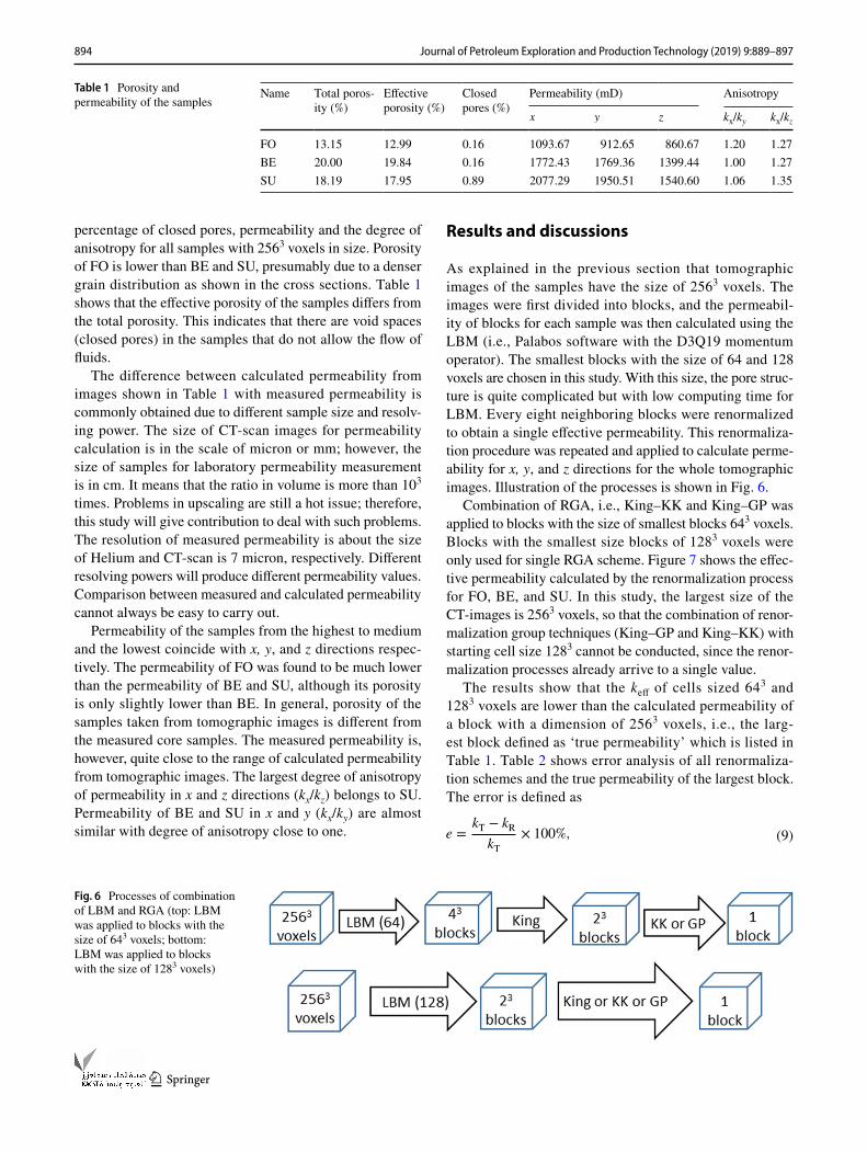
As explained in the previous section that tomographic images of the samples have the size of 2563 voxels. The images were first divided into blocks, and the permeabil-ity of blocks for each sample was then calculated using the LBM (i.e., Palabos software with the D3Q19 momentum operator). The smallest blocks with the size of 64 and 128 voxels are chosen in this study. With this size, the pore struc-ture is quite complicated but with low computing time for LBM. Every eight neighboring blocks were renormalized to obtain a single effective permeability. This renormaliza-tion procedure was repeated and applied to calculate perme-ability for x, y, and z directions for the whole tomographic images. Illustration of the processes is shown in Fig. 6.

Combination of RGA, i.e., King–KK and King–GP was applied to blocks with the size of smallest blocks 643 voxels. Blocks with the smallest size blocks of 1283 voxels were only used for single RGA scheme. Figure 7 shows the effec-tive permeability calculated by the renormalization process for FO, BE, and SU. In this study, the largest size of the CT-images is 2563 voxels, so that the combination of renor-malization group techniques (King–GP and King–KK) with starting cell size 1283 cannot be conducted, since the renor-malization processes already arrive to a single value.

The results show that the keff of cells sized 643 and 1283 voxels are lower than the calculated permeability of a block with a dimension of 2563 voxels, i.e., the larg-est block defined as ‘true permeability’ which is listed in Table 1. Table 2 shows error analysis of all renormaliza-tion schemes and the true permeability of the largest block. The error is defined as

(9)e =kT − kR

kT× 100%,

Table 1 Porosity and permeability of the samples

Name Total poros-ity (%)

Effective porosity (%)

Closed pores (%)

Permeability (mD) Anisotropy

x y z kx/ky kx/kz

FO 13.15 12.99 0.16 1093.67 912.65 860.67 1.20 1.27BE 20.00 19.84 0.16 1772.43 1769.36 1399.44 1.00 1.27SU 18.19 17.95 0.89 2077.29 1950.51 1540.60 1.06 1.35

Fig. 6 Processes of combination of LBM and RGA (top: LBM was applied to blocks with the size of 643 voxels; bottom: LBM was applied to blocks with the size of 1283 voxels)

895Journal of Petroleum Exploration and Production Technology (2019) 9:889–897

1 3

where kR is the permeability after renormalization scheme and kT is the true permeability.

It seems that almost all of permeability values after renor-malization processes are lower than the true permeability. In general, the closest effective permeability to the true perme-ability for almost all samples in all directions was produced by Karim and Krabbenhoft’s (KK) renormalization scheme. The KK scheme does not give closest results for sample SU, but still produces quite low error (less than 15%).

Interestingly the ratio in all directions for different initial block sizes (i.e., kx − 64/kx − 128, kx − 128/kx − 256 and also

in the direction of y and z) for almost all of the samples is similar in the range of 0.8–1.0. The plots of the degree of anisotropy against the RGA schemes are shown in Fig. 8.

Comparing degree of anisotropy plotted in Fig. 8a, b, we can see that the degree of anisotropy in the z-direc-tion (kx/kz) was greater than the degree of anisotropy in the y-direction (kx/ky). The results show that size of the smallest block for RGA influenced the degree of anisot-ropy. Blocks with the size of 643 voxels as starting block for RGA have higher degree of anisotropy than blocks with the size of 1283 and 2563 voxels. Investigation on

Fig. 7 Effective permeability after renormalization processes

0

500

1000

1500

2000

2500

perm

eabi

lity

(mD)

Effec�ve permeability

x-064

y-064

z-064

x-128

y-128

z-128

x-256

y-256

z-256

FO

BE SU

Table 2 Error analysis of all renormalization schemes which are calculated using Eq. 9

No Technique Cells size = 643 voxels Cells size = 1283 voxels Error cell of k for size 64

Error of k for cell size 128

x y z x y z x (%) y (%) z (%) x (%) y (%) z (%)

FO1 King 892.8 653.81 523.17 1134.33 807.21 720.08 18.37 28.36 39.21 − 3.72 11.55 16.332 Green and Paterson 871.03 620.1 498.25 1125.17 792.56 709.88 20.36 32.06 42.11 − 2.88 13.16 17.523 Karim and Krabbenhoft 973.34 723.63 586.75 1156.88 811.59 733.43 11.00 20.71 31.83 − 5.78 11.07 14.784 King–GP 882.28 641.72 512.57 NA NA NA 19.33 29.69 40.45 NA NA NA5 King–KK 909.93 671.93 532.84 NA NA NA 16.80 26.38 38.09 NA NA NABE1 King 1514.21 1294.79 1155.08 1684.09 1597.19 1252.26 14.57 26.82 17.46 4.98 9.73 10.522 Green and Paterson 1491.59 1243.75 1125.76 1677.1 1584.98 1247.41 15.84 29.71 19.56 5.38 10.42 10.863 Karim and Krabbenhoft 1429.46 1417.25 1233.85 1683.47 1598.91 1260.3 19.35 19.90 11.83 5.02 9.63 9.944 King–GP 1508.5 1281.79 1152.79 NA NA NA 14.89 27.56 17.62 NA NA NA5 King–KK 1518.94 1308.24 1156.93 NA NA NA 14.30 26.06 17.33 NA NA NASU1 King 1841.52 1535.87 1234.14 1913.52 1777.53 1562.78 11.35 21.26 19.89 7.88 8.87 − 1.442 Green and Paterson 1891.54 1771.59 1550.61 1785.67 1464.37 1186.14 8.94 9.17 − 0.65 14.04 24.92 23.013 Karim and Krabbenhoft 1950.55 1644.31 1358.74 1910.07 1779.71 1571.8 6.10 15.70 11.80 8.05 8.76 − 2.034 King–GP 1829.63 1527.18 1218.93 NA NA NA 11.92 21.70 20.88 NA NA NA5 King–KK 1840.09 1540.41 1256.3 NA NA NA 11.42 21.03 18.45 NA NA NA

896 Journal of Petroleum Exploration and Production Technology (2019) 9:889–897

1 3

variation in the petrophysical parameters with the size of the selected sub-volume (either 512 or 1024 voxels) using LBM showed that homogeneous sandstones give the same results for the two subset sizes (Alyafei et al. 2016). Compromise between the representative sample size and the pixel resolution of the CT scans, especially regarding heterogeneities of the sampled material, will still be chal-lenging (Cnudde and Boone 2013; Henkel et al. 2016). Applicability of this method to carbonate rocks with more complicated and heterogeneous pore space (Krakowska et al. 2016; Nurgalieva and Nurgalieva 2016) as mentioned by many authors, are also encouraging.

Conclusions

The effective permeability calculated by means of RGA was lower than LBM for a single block with a dimension of 2563 voxels. The keff produced by Karim and Krabbenhoft’s renormalization technique are mostly the closest to the true permeability. The degree of anisotropy showed that FO, BE, and SU are slightly anisotropic, where the degree of anisot-ropy (i.e., kx/kz) is larger than the kx/ky. Degree of anisotropy seems to be influenced by initial block size for RGA.

Acknowledgements We would like to thank Doctoral Research Grant from the Directorate for Higher Education of Republic of Indonesia for financial support and LEMIGAS for providing Sumatra’s rock sample.

Open Access This article is distributed under the terms of the Crea-tive Commons Attribution 4.0 International License (http://creat iveco mmons .org/licen ses/by/4.0/), which permits unrestricted use, distribu-tion, and reproduction in any medium, provided you give appropriate credit to the original author(s) and the source, provide a link to the Creative Commons license, and indicate if changes were made.

References

Aharony A, Hinrichsen EL, Hansen A, Feder J, Hardy H (1991) Effec-tive renormalization group algorithm for transport in oil reser-voirs. Phys A 177:260–266

Alyafei N, Mckay TJ, Solling TI (2016) Characterization of petrophysi-cal properties using pore-network and lattice-Boltzmann model-ling: choice of method and image sub-volume size. J Petrol Sci Eng 145:256–265

Cnudde V, Boone MN (2013) High-resolution X-ray computed tomog-raphy in geosciences: a review of the current technology and applications. Earth Sci Rev 123:1–17

De Paoli M, Zonta F, Soldati A (2016) Influence of anisotropic perme-ability on convection in porous media: implications for geological CO2 sequestration. Phys Fluids 28:056601

Dong H (2008) Micro-CT imaging and pore network extraction. Department of Earth Science and Engineering, Imperial College, London

Farquharson JI, Heap MJ, Lavallée Y, Varley NR, Baud P (2016) Evi-dence for the development of permeability anisotropy in lava domes and volcanic conduits. J Volcanol Geoth Res 323:163–185

Fauzi U (2011) An estimation of rock permeability and its anisotropy from thin sections using a renormalization group approach. Energy Sourc Part A Recov Utilization Environ Effects 33:539–548

Green CP, Paterson L (2007) Analytical three-dimensional renormali-zation for calculating effective permeabilities. Transp Porous Media 68:237–248

Henkel S, Pudlo D, Enzmann F, Reitenbach V, Albrecht D, Ganzer L, Gaupp R (2016) X-ray CT analyses, models and numerical simu-lations: a comparison with petrophysical analyses in an experi-mental CO2 study. Solid Earth 7(3):917–927

Iscan A, Kok M (2009) Porosity and permeability determinations in sandstone and limestone rocks using thin section analysis approach. Energy Sourc Part A 31:568–575

Jin G, Patzek TW, Silin DB (2004) Direct prediction of the absolute permeability of unconsolidated and consolidated reservoir rock. In: SPE annual technical conference and exhibition society of petroleum engineers

Kameda A, Dvorkin J (2004) Permeability in the thin section. In: SEG technical program expanded abstracts 2004. Society of exploration geophysicists, pp 1706–1709

a Permeability anisotropy for kx/kz. b Permeability anisotropy for kx/ky.

0.800.901.001.101.201.301.401.501.601.701.80

King GP KK

King

-GP

King

-KK

King GP KK

King

-GP

King

-KK

King GP KK

King

-GP

King

-KK

Degr

ee o

f ani

sotr

opy

Permeability Anisotropy (kx/kz)

kx/kz-64 kx/kz-128 kx/kz-256 FO

kx/kz-256 BE kx/kz-256 SU

0.800.901.001.101.201.301.401.50

King GP KK

King

-GP

King

-KK

King GP KK

King

-GP

King

-KK

King GP KK

King

-GP

King

-KK

Degr

ee o

f ani

sotr

opy

Permeability Anisotropy (kx/ky)

kx/ky-64 kx/ky-128 kx/ky-256 FO

kx/ky-256 BE kx/ky-256 SU

FO BE SU FO BE SU

Fig. 8 Permeability anisotropy of the samples

897Journal of Petroleum Exploration and Production Technology (2019) 9:889–897

1 3

Karim M, Krabbenhoft K (2010) New renormalization schemes for conductivity upscaling in heterogeneous media. Transp Porous Media 85:677–690

Khalili AD et al (2012) Permeability upscaling for carbonates from the pore-scale using multi-scale Xray-CT images. In: SPE/EAGE European unconventional resources conference & exhibition-from potential to production

King P (1989) The use of renormalization for calculating effective permeability. Transp Porous Media 4:37–58

Krakowska P, Dohnalik M, Jarzyna J, Wawrzyniak-Guz K (2016) Com-puted X-ray microtomography as the useful tool in petrophysics: a case study of tight carbonates Modryn formation from Poland. J Nat Gas Sci Eng 31:67–75

Kutay M, Aydilek A (2005) Lattice Boltzmann method for modeling fluid flow through asphalt concrete. Environmental Geotechnics Report No 05:2

Latief F, Biswal B, Fauzi U, Hilfer R (2010) Continuum reconstruction of the pore scale microstructure for Fontainebleau sandstone. Phys A 389:1607–1618

Liu J, Pereira GG, Regenauer-Lieb K (2014) From characterisation of pore-structures to simulations of pore-scale fluid flow and the

upscaling of permeability using microtomography: a case study of heterogeneous carbonates. J Geochem Explor 144:84–96

Liu J, Pereira GG, Liu Q, Regenauer-Lieb K (2016) Computational challenges in the analyses of petrophysics using microtomography and upscaling. A review. Comput Geosci 89:107–117

Nurgalieva ND, Nurgalieva NG (2016) New digital methods of estima-tion of porosity of carbonate rocks. Indian J Sci Technol. https ://doi.org/10.17485 /ijst/2016/v9i20 /93750

Rama P et al (2011) Determination of the anisotropic permeability of a carbon cloth gas diffusion layer through X-ray computer micro-tomography and single-phase lattice Boltzmann simulation. Int J Numer Methods Fluids 67:518–530

Wright H, Roberts JJ, Cashman KV (2006) Permeability of anisotropic tube pumice: model calculations and measurements. Geophys Res Lett. https ://doi.org/10.1029/2006G L0272 24

Publisher’s Note Springer Nature remains neutral with regard to jurisdictional claims in published maps and institutional affiliations.