Embed Size (px)
Citation preview

CALCULATING ITEM DISCRIMINATION VALUES USING SAMPLES OF
EXAMINEE SCORES AROUND REAL AND ANTICIPATED CUT SCORES: EFFECTS ON ITEM DISCRIMINATION, ITEM SELECTION, EXAMINATION RELIABILITY,
AND CLASSIFICATION DECISION CONSISTENCY
Darin S. Earnest
A dissertation submitted to the faculty at the University of North Carolina at Chapel Hill in partial fulfillment of the requirements for the degree of Doctor of Philosophy in the
School of Education.
Chapel Hill 2014
Approved by: Gregory J. Cizek Gary S. Cuddeback Jeffrey A. Greene Stephen Johnson William B. Ware

ii
© 2014
Darin S. Earnest ALL RIGHTS RESERVED

iii
ABSTRACT
Darin S. Earnest: Calculating item discrimination values using samples of examinee scores around real and anticipated cut scores: Effects on item discrimination, item selection,
examination reliability, and classification decision consistency (Under the direction of Gregory J. Cizek)
This study examined the degree to which limiting the calculation of item
discrimination values to groups of examinee scores near real and anticipated cut scores
affected item discrimination, item selection, examination reliability, and classification
decision consistency. Three examinations used to credential individuals in health-related
professions were used to answer the research questions. To replicate as closely as possible
the context in which many credentialing examinations are developed, each of the
examinations consisted of small samples of examinees and were analyzed using classical test
theory procedures.
Item discrimination values, as expressed by the point-biserial statistic, were
calculated for each examination item. Restricted item discrimination values were then
calculated for each item using subsets of examinee scores. The restricted values were based
on scores within 0.50 SD, 0.75 SD, and 1.00 SD of five unique cut score locations.
Differences between unrestricted and restricted item discrimination values were measured.
Two 50-item test variants for each examination were created to evaluate the effect restricted
item discrimination values had on item selection, examination reliability, and classification
decision consistency. Form A variants included the 50 most discriminating items using

iv
unrestricted discrimination values. Form B variants included the 50 most discriminating
items using restricted discrimination values.
The results of the study indicated that (a) item discrimination values were lower when
their calculation was limited to groups of scores near cut scores; (b) using restricted item
discrimination values as the criterion by which items were selected for test variants resulted
in the selection of items that were different than those selected when unrestricted values were
used as the selection criterion; (c) differences in examination reliability between test variants
were found to be statistically significant, with scores of variants based on restricted item
discrimination values producing lower estimates; and (d) test variants based on restricted
item discrimination values produced slightly lower observed classification decision
consistency estimates than variants based on unrestricted item discrimination values. The
results of the study were tied to several aspects of the test development process for
credentialing examinations, including issues related to sample size, cut score location, and
examination validity.

v
To my family.

vi
ACKNOWLEDGEMENTS
Many people have supported me throughout this process. First, I could not have been
successful in completing this journey without the love and encouragement of my wife,
Annee. For your continual support and understanding, I am truly grateful. Thank you,
Henry, George, Jane, Ruby, Eleanor, and Walter for letting me work when I needed to and
for motivating me each and every day.
I am also grateful for the amazing and steadfast support of my advisor and mentor,
Dr. Gregory Cizek. Thank you for believing in me and for your invaluable advice. I would
also like to thank the members of my dissertation committee: Dr. Gary Cuddeback, Dr.
Jeffrey Greene, Dr. Stephen Johnson, and Dr. William Ware. I truly appreciate the assistance
and feedback that each provided me throughout this process.
Finally, thank you to the leadership and faculty of the Department of Foreign
Languages at the United States Air Force Academy for giving me this opportunity. It is my
great honor and privilege to serve with you.

vii
TABLE OF CONTENTS
LIST OF TABLES.....................................................................................................................x LIST OF FIGURES................................................................................................................xiii CHAPTER 1: INTRODUCTION.............................................................................................1 Research Questions........................................................................................................7 Need for the Study.........................................................................................................7 CHAPTER 2: LITERATURE REVIEW................................................................................10
Item Discrimination and the Test Development Process.............................................10
Credentialing Examinations.........................................................................................22
Test Development with Small Samples of Examinee Responses................................36
Summary......................................................................................................................38
CHAPTER 3: METHOD........................................................................................................40
Participants...................................................................................................................40
Materials......................................................................................................................41
Examination 1..................................................................................................41
Examination 2..................................................................................................45
Examination 3..................................................................................................46
Data Analysis...............................................................................................................47
Research Question 1........................................................................................49
Research Question 2........................................................................................56

viii
CHAPTER 4: RESULTS........................................................................................................62
Research Question 1....................................................................................................62
Examination 1..................................................................................................64
Examination 2..................................................................................................78
Examination 3..................................................................................................90
Summary – Research Question 1...................................................................102
Research Question 2..................................................................................................103
Examination 1................................................................................................103
Examination 2................................................................................................108
Examination 3................................................................................................111
Summary – Research Question 2...................................................................113 CHAPTER 5: DISCUSSION................................................................................................115 Limitations.................................................................................................................115
Refinement of Items Used in the Study.........................................................116
Item Selection Criteria...................................................................................117
Key Findings..............................................................................................................120
Effect on Item Discrimination Values...........................................................121
Effect on Item Selection.................................................................................127
Effect on Examination Reliability.................................................................130
Effect on Classification Decision Consistency..............................................134
Recommendations for Future Research.....................................................................135
Conduct Research with Less Refined Items..................................................136
Use Test Specifications to Guide Item Selection...........................................136

ix
Develop Longer Tests to Assess Effects of Restricted Discrimination Values...................................................................................137
Use of Non-Classical Test Theory Approaches.............................................138
Effects of Restricted Discrimination Values on Standard Setting.................139
Conclusion.................................................................................................................139
APPENDIX A: ITEM DISCRIMINATION VALUES – EXAMINATION 1....................142
APPENDIX B: ITEM DISCRIMINATION VALUES – EXAMINATION 2.....................172
APPENDIX C: ITEM DISCRIMINATION VALUES – EXAMINATION 3.....................207
REFERENCES......................................................................................................................232

x
LIST OF TABLES
Table 1.1 - Test Development Process......................................................................................4 Table 2.1 - States with Most and Fewest Licensed Occupations ............................................25 Table 3.1 - Summary of Examination Characteristics.............................................................41 Table 3.2 - Descriptive Statistics for Examinations Used.......................................................44 Table 3.3 - R Packages Used to Complete Procedures...........................................................48 Table 3.4 - Description of Item Discrimination Values Calculated........................................53 Table 4.1 - Conditions for the Calculation of Restricted Point-biserials................................63 Table 4.2 - Descriptive Statistics of Discrimination Values
Calculated for Examination 1...............................................................................72 Table 4.3 - Correlation Matrix of Item Discrimination Values
Calculated for Examination 1...............................................................................73 Table 4.4 - Results of the One-way Repeated Measures ANOVA for Examination 1...........75 Table 4.5 - Results of Tukey’s HSD Test for Examination 1
- Unrestricted vs. Restricted Values......................................................................77 Table 4.6 - Descriptive Statistics of Discrimination Values
Calculated for Examination 2...............................................................................85 Table 4.7 - Correlation Matrix of Item Discrimination Values
Calculated for Examination 2...............................................................................87 Table 4.8 - Results of the One-way Repeated Measures ANOVA for Examination 2............88 Table 4.9 - Results of Tukey’s HSD Test for Examination 2 - Unrestricted vs. Restricted Values......................................................................89 Table 4.10 - Descriptive Statistics of Discrimination Values
Calculated for Examination 3.............................................................................97 Table 4.11 - Correlation Matrix of Item Discrimination Values Calculated for Examination 3.............................................................................99 Table 4.12 - Results of the One-way Repeated Measures ANOVA for Examination 3........100

xi
Table 4.13 - Results of Tukey’s HSD Test for Examination 3 - Unrestricted vs. Restricted Values..................................................................101 Table 4.14 - Descriptive Statistics of Test Forms A and B – All Examinations...................104 Table 4.15 - Items and Discrimination Values for Form A and Form B – Examination 1....................................................................................105 Table 4.16 - Descriptive Statistics of Form A and Form B Discrimination Values – Examination 1....................................................................................106 Table 4.17 - Items and Discrimination Values for Form A and Form B – Examination 2....................................................................................109 Table 4.18 - Descriptive Statistics of Form A and Form B Discrimination Values – Examination 2....................................................................................110 Table 4.19 - Items and Discrimination Values for Form A and Form B – Examination 3....................................................................................112 Table 4.20 - Descriptive Statistics of Form A and Form B Discrimination Values – Examination 3....................................................................................113 Table 5.1 - Descriptive Statistics of Discrimination Values – All Examinations..................122 Table 5.2 - Change in Direction of Discrimination Values – All Examinations...................124 Table 5.3 - Descriptive Statistics of Selected Groups of Scores............................................127 Table 5.4 - Descriptive Statistics of Forms A and B Test Variants – All Examinations.......128 Table 5.5 - Descriptive Statistics for Unique Form A and Form B Test Variant Items – All Examinations..................................................132 Table A.1 - Item Discrimination Values for Examination 1 – CX1........................................142 Table A.2 - Item Discrimination Values for Examination 1 – CX2........................................148 Table A.3 - Item Discrimination Values for Examination 1 – CX3........................................154 Table A.4 - Item Discrimination Values for Examination 1 – CX4........................................160 Table A.5 - Item Discrimination Values for Examination 1 – CX5........................................166 Table B.1 - Item Discrimination Values for Examination 2 – CX1........................................172
xii
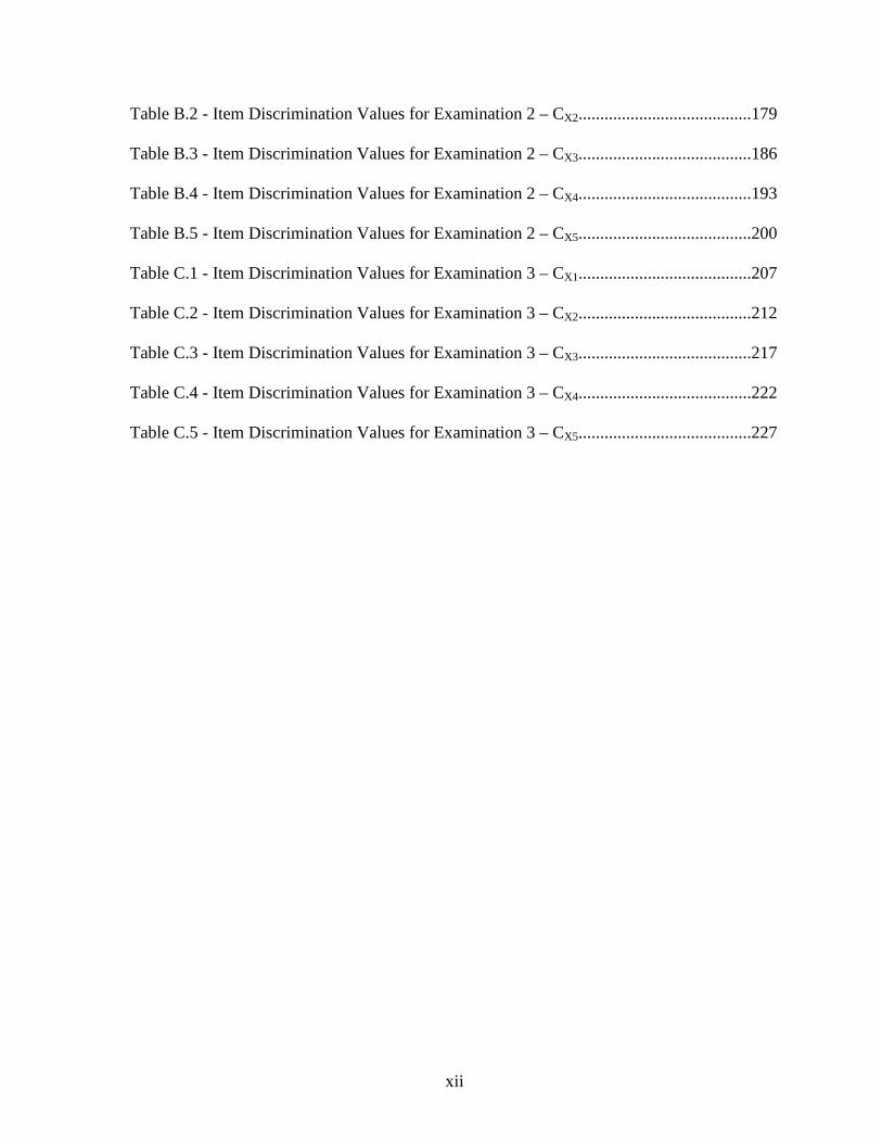
Table B.2 - Item Discrimination Values for Examination 2 – CX2........................................179 Table B.3 - Item Discrimination Values for Examination 2 – CX3........................................186 Table B.4 - Item Discrimination Values for Examination 2 – CX4........................................193 Table B.5 - Item Discrimination Values for Examination 2 – CX5........................................200 Table C.1 - Item Discrimination Values for Examination 3 – CX1........................................207 Table C.2 - Item Discrimination Values for Examination 3 – CX2........................................212 Table C.3 - Item Discrimination Values for Examination 3 – CX3........................................217 Table C.4 - Item Discrimination Values for Examination 3 – CX4........................................222 Table C.5 - Item Discrimination Values for Examination 3 – CX5........................................227

xiii
LIST OF FIGURES
Figure 2.1 - Example of item characteristic curve (ICC).........................................................18
Figure 2.2 - Probabilities of consistent classifications using two forms..................................32
Figure 3.1 - Histogram of total scores for Examination 1.......................................................43
Figure 3.1 - Histogram of total scores for Examination 2.......................................................45
Figure 3.1 - Histogram of total scores for Examination 3.......................................................47
Figure 4.1 - Plots of unrestricted and restricted item discrimination values based on scores within 1.00 SD, 0.75 SD, and 0.50 SD of CX1 for Examination 1............65 Figure 4.2 - Plots of unrestricted and restricted item discrimination values based on scores within 1.00 SD, 0.75 SD, and 0.50 SD of CX2 for Examination 1............66 Figure 4.3 - Plots of unrestricted and restricted item discrimination values based on scores within 1.00 SD, 0.75 SD, and 0.50 SD of CX3 for Examination 1............67 Figure 4.4 - Plots of unrestricted and restricted item discrimination values based on scores within 1.00 SD, 0.75 SD, and 0.50 SD of CX4 for Examination 1............68 Figure 4.5 - Plots of unrestricted and restricted item discrimination values based on scores within 1.00 SD, 0.75 SD, and 0.50 SD of CX5 for Examination 1............69 Figure 4.6 - Boxplot highlighting distribution of item discrimination values under each condition for Examination 1........................................................................70 Figure 4.7 - Plots of unrestricted and restricted item discrimination values based on scores within 1.00 SD, 0.75 SD, and 0.50 SD of CX1 for Examination 2............79 Figure 4.8 - Plots of unrestricted and restricted item discrimination values based on scores within 1.00 SD, 0.75 SD, and 0.50 SD of CX2 for Examination 2............80 Figure 4.9 - Plots of unrestricted and restricted item discrimination values based on scores within 1.00 SD, 0.75 SD, and 0.50 SD of CX3 for Examination 2............81 Figure 4.10 - Plots of unrestricted and restricted item discrimination values based on scores within 1.00 SD, 0.75 SD, and 0.50 SD of CX4 for Examination 2..........82 Figure 4.11 - Plots of unrestricted and restricted item discrimination values based on scores within 1.00 SD, 0.75 SD, and 0.50 SD of CX5 for Examination 2..........83

xiv
Figure 4.12 - Boxplot highlighting distribution of item discrimination values under each condition for Examination 2......................................................................84 Figure 4.13 - Plots of unrestricted and restricted item discrimination values based on scores within 1.00 SD, 0.75 SD, and 0.50 SD of CX1 for Examination 3..........91 Figure 4.14 - Plots of unrestricted and restricted item discrimination values based on scores within 1.00 SD, 0.75 SD, and 0.50 SD of CX2 for Examination 3..........92 Figure 4.15 - Plots of unrestricted and restricted item discrimination values based on scores within 1.00 SD, 0.75 SD, and 0.50 SD of CX3 for Examination 3..........93 Figure 4.16 - Plots of unrestricted and restricted item discrimination values based on scores within 1.00 SD, 0.75 SD, and 0.50 SD of CX4 for Examination 3..........94 Figure 4.17 - Plots of unrestricted and restricted item discrimination values based on scores within 1.00 SD, 0.75 SD, and 0.50 SD of CX5 for Examination 3..........95 Figure 4.18 - Boxplot highlighting distribution of item discrimination values under each condition for Examination 3......................................................................96 Figure 5.1 - Pie charts representing breakdown of Form B test variant items for each
examination.......................................................................................................129 Figure 5.2 - Pass/fail consistency tables for Examination 1 and associated test variants................................................................................131 Figure 5.3 - Pass/fail consistency tables for Examination 2 and associated test variants................................................................................132 Figure 5.4 - Pass/fail consistency tables for Examination 3 and associated test variants................................................................................133

1
CHAPTER 1
INTRODUCTION
Examinations, and the roles they play in a variety of fields, have been the source of
much debate in recent years. In the educational setting, for example, legislation like the 2001
No Child Left Behind Act (NCLB, 2002) shifted significant attention to student performance
on mandatory end-of-grade examinations. The results of these examinations, depending on
location, are often taken into consideration when important school-related decisions such as
student retention and educator evaluation and compensation are made. In some areas, the
results can even affect school and school district operating budgets.
Increased focus on the use of examinations in schools has led to greater scrutiny of
the process by which these tests are developed. Ensuring that examinations are valid and
reliable is in the interest of all who are affected by their results. To that end, the American
Educational Research Association (AERA), the American Psychological Association (APA),
and the National Council on Measurement in Education (NCME) jointly developed and
published the Standards for Educational and Psychological Testing (1999; hereafter,
Standards). According to the Standards, “The proper use of tests can result in wiser
decisions about individual programs than would be the case without their use and also can
provide a route to broader an more equitable access to education and employment” (p. 1).
The intent of the Standards is to “promote the sound and ethical use of tests” and to provide a
basis for “evaluating the quality of testing practices” (p. 1).
2
Education is not the only field, however, in which the results of examinations can be
significant and consequential. Government agencies and other professional organizations
frequently require applicants for credentials to pass license- or certification-granting
examinations. Lawyers, physicians, electricians, and barbers are all examples of
professionals who are required to receive government-issued licenses before being authorized
to practice in their respective fields. Likewise, non-governmental entities often use
examinations as part of the process to certify persons to perform tasks or operations that
require specific skill sets. An information technology company, for instance, may require
technicians to pass an examination before authorizing them to work on certain software
programs. Tests that are used to grant certifications or award professional recognitions are
frequently referred to as credentialing examinations.
Like other types of tests, credentialing examinations need to be developed in a
manner that ensures their results produce desired thresholds of validity and reliability.
According to the Standards (AERA, APA, & NCME, 1999), “Tests and testing programs
should be developed on a strong scientific basis. Test developers and publishers should
compile and document adequate evidence bearing on test development” (p. 43). In addition
to the guidelines listed in the Standards, credentialing examinations may also be required to
meet additional criteria. Depending on the nature of the organization using the examination,
compliance with guidelines set forth by national and international standards organizations,
such as the American National Standards Institute (ANSI; 2013) and the International
Organization for Standardization (ISO; 2013) may also be desired or required.
Standardization organizations such as these ensure that licensure and certification

3
requirements are consistent among relevant parties. Adhering to these standards may also
provide legal defensibility for the developers and administrators of these examinations.
The process by which credentialing examinations are developed is similar to that
which is used for other types of tests. According to Downing (2006), the typical test
development process is comprised of 12 steps. These steps are included in Table 1.1. The
process begins with gaining an understanding of the purpose of the examination, the desired
inferences to be made by test scores, as well as the general format to be used. Additional
steps include defining the content to be used, creating test specifications, developing
examination items, designing and assembling the test, and test production. Following these
procedures, items are frequently field-tested, scored, and analyzed to judge the
appropriateness of their inclusion in final versions of examinations. If applicable, a standard
setting process may be used to recommend a minimum passing score for the test. This is
followed by the development of a test reporting protocol, the establishment of an
examination item bank, and the creation of technical reports that document the development
process. Each step in this process is as important as the next and frequently serves as
evidence for claims of examination validity.

4
Table 1.1
Test Development Process Step Examples of development tasks and concerns 1. Overall plan Guidance for test development activities Confirm desired test interpretations Test format 2. Content definition Sampling plan Content-related validity evidence 3. Test specifications Content domain sampling Desired item characteristics 4. Item development Item writer training Item review, editing 5. Test design and assembly Design/create test forms Develop pretesting considerations 6. Test production Publishing/printing activities Security/quality control 7. Test administration Standardization issues Proctoring, security, timing issues 8. Scoring test responses Quality control Item analysis 9. Passing scores Standard setting Comparability of standards 10. Reporting test results Accuracy, quality control Misuse/retake issues 11. Item banking Security issues Usefulness, flexibility 12. Test technical report Documentation of validity evidence Recommendations Note. Test development steps adapted from Downing (2006).
5
The development process for credentialing examinations can be affected by the
unique characteristics these tests frequently exhibit. Unlike large-scale standardized tests
used in education, credentialing examinations are often developed and administered for
organizations representing occupations or fields with relatively few potential members. As
such, the resources these groups are able to devote to test development and administration
may be relatively limited. Although not wholly unique to credentialing examinations,
examinees seeking a license or certification must also typically reach a predetermined
minimum score, or cut score, in order to pass the examination and, therefore, be eligible to
receive the desired credential. Tests with cut scores are also sometimes referred to as
competency or mastery examinations because obtaining a score at or higher than the cut
score infers examinee mastery or competency over a specified set of content standards.
These attributes make credentialing examinations different than many standardized tests used
in education, such as those used to measure the aptitude of prospective first-year college
students. Such examinations are administered to thousands of examinees each year, creating
large sets of data by which the development process is significantly aided.
The focus of this study is on one step in the process used to develop credentialing
examinations. This step, frequently referred to as item analysis, is used to assess the degree
to which field-tested items are suitable for inclusion in final versions of examinations. Item
analysis, which Crocker and Algina (2008) defined as “the computation and examination of
any statistical property of examinees’ responses to an individual test item” is included in Step
6 of Downing’s (2006) development process (p. 311). The statistical properties most
commonly used to assess individual examination items are item difficulty which, in classical
test theory (CTT) terms, is the proportion of examinees that respond to an item correctly; and

6
item discrimination, which measures the degree to which an item differentiates between
examinees who possess more of some characteristic intended to be measured by a test (e.g.,
subject area mastery) and those who possess less of the characteristic. This differentiation is
typically operationalized as the difference between those examinees who perform relatively
well on an examination and those who perform relatively poorly.
The procedures used to calculate item discrimination values for credentialing
examinations with relatively small samples of field-test data are the focus of this study. A
number of statistics are currently used to gauge item discrimination. A common
characteristic among these methods, however, is that in calculating the discrimination values
they consider scores from all examinees. In this study, discrimination values calculated
using these traditional methods are referred to as unrestricted, because they incorporate data
from all examinees. This research studies the effects of limiting the data used to calculate
item discrimination to that of examinees who score around the test cut score. These values
are referred to as restricted because they consider only a limited subset of examinee scores.
In addition to examining how restricting scores used in the calculation of discrimination
values affects the values themselves, the study investigates the effects of restricted
discrimination values on certain aspects of test development, including item selection,
examination reliability, and classification decision consistency.

7
Research Questions
The following research questions are addressed in this study:
1. What are the effects on item discrimination values when the values are calculated using
restricted samples of examinee test scores within varying ability ranges around real or
anticipated cut scores?
2. What are the effects of calculating item discrimination values based on varying ranges of
examinees around cut scores on item selection, examination reliability, and classification
decision consistency?
Need for the Study
The current study represents a unique contribution to the field of test development for
credentialing examinations. Current procedures used to calculate item discrimination values,
although appropriate and effective for many types of tests, may not be ideal for competency
examinations. In addition, the study’s emphasis on tests with small samples of examinees
represents the realistic—and under-studied—conditions of many testing programs,
particularly those used by credential-granting organizations. Using small sample sizes also
necessitates the use of classical test theory procedures, which, despite the emergence of more
sophisticated measurement models, remain popular among developers of credentialing
examinations. Some of the important potential benefits of this study are described in the
following paragraphs.
First, although a variety of procedures may be used to calculate item discrimination
values, a common characteristic of these procedures is that they each use the entire
population of previous examinees as the criterion group when calculating the discrimination

8
values. In this manner, they treat scores of examinees at both the extreme upper and lower
ends of a distribution of test scores as they do scores from examinees near the examination
cut score. The focus of competency examinations, however, is on candidates near the cut
score. By limiting the basis for calculating discrimination values to scores of examinees near
the actual or estimated cut score, greater emphasis may be applied to items that discriminate
more effectively amongst examinees with ability levels closest to those for which the test was
designed to distinguish.
If the sample of examinees on which discrimination values are calculated is restricted,
the restriction is likely to affect the selection of items for competency examinations. It is
expected that discrimination indices based on criterion groups having a narrower range of
ability or performance would produce uniformly attenuated discrimination indices.
However, if discrimination values based on responses within a restricted sample of
examinees are significantly different than those calculated using all examinees, the items
selected for an examination will be dependent on the method employed. In other words,
restricting the range of test scores used to calculate discrimination values permits items that
discriminate among examinees with ability levels closest to those the cut score
operationalizes to be selected over those that discriminate in other areas within the range of
test scores.
The degree to which limiting the calculation of item discrimination values to scores
of examinees around cut scores affects other aspects of test development also warrants
further research. This study specifically examines how calculating discrimination values in
this manner affects examination reliability and classification decision consistency.

9
Second, an important aspect of this research is that it was conducted within the
context of competency examinations with relatively small numbers of examinees. Limiting
the research to small-sample examinations is of particular benefit to developers of tests used
to credential individuals. Unlike many large-scale educational achievement examinations for
which item analysis may rely on large numbers of student responses and test scores,
credentialing tests, due to their very nature, are often limited to smaller pools of examinees.
Much of the research related to item analysis has focused on tests with large numbers of
examinees. Fewer, however, have examined these issues as they specifically relate to
examinations with smaller samples of available test scores. Focusing the study in this
manner represents a significant contribution to small-sample examination development.
Finally, whereas the research presented here focused on examinations with small
samples of response data, classical test theory procedures were appropriate and were used
throughout. These procedures, though less computationally complex than more recent
measurement theories, are still widely used by those responsible for developing credentialing
examinations. The results of classical test theory-based procedures are also frequently
viewed as being easier to interpret by individuals without backgrounds in measurement
theory or statistics than the more complex models. As such, the results of this study are
generalizable to a large segment of the test development field.

10
CHAPTER 2
LITERATURE REVIEW
The subjects addressed in this study draw upon relevant literature from three major
areas of research: (a) analyses regarding item discrimination and its role in the test
development process, (b) studies pertaining to the development of mastery or competency
examinations used to credential individuals, and (c) research related to test development
when relatively small samples of examinee scores are available. Significant research from
each of these three areas is described in the sections that follow.
Item Discrimination and the Test Development Process
Assessing the degree to which items discriminate between examinees who possess
more of some knowledge, skill, or ability and those who exhibit less is an important element
in the process by which items are selected for inclusion in all types of examinations. This
process, commonly referred to as item analysis, is used to compute the statistical properties
of examinee responses to individual test items (Crocker & Algina, 2008). The goal of item
analysis is to ensure that items selected for examinations yield levels of reliability and
validity that sufficiently support the test’s intended purpose. Items that discriminate between
high- and low-performing examinees are typically viewed as being desirable and, as such,
worthy of being included in an examination; items that do not are frequently removed from
consideration for inclusion in an examination.
11
Many item discrimination methods have been developed to assess the relationship
between examinee responses to individual test items and test performance. Although the
approaches used to calculate discrimination values according to these indices vary, they share
a common purpose: to identify test items to which high-scoring examinees have a high
probability of responding correctly, and to which low-scoring examinees have a low
probability of responding correctly. A description of commonly used item discrimination
indices is included in the sections that follow.
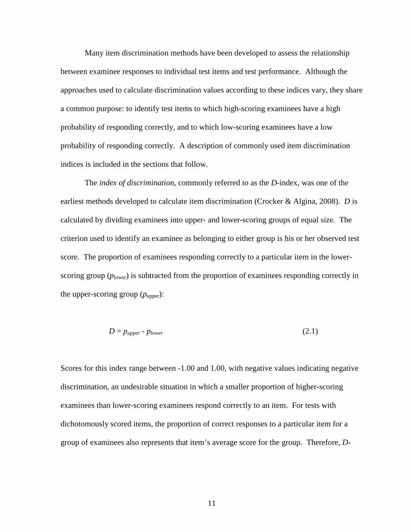
The index of discrimination, commonly referred to as the D-index, was one of the
earliest methods developed to calculate item discrimination (Crocker & Algina, 2008). D is
calculated by dividing examinees into upper- and lower-scoring groups of equal size. The
criterion used to identify an examinee as belonging to either group is his or her observed test
score. The proportion of examinees responding correctly to a particular item in the lower-
scoring group (plower) is subtracted from the proportion of examinees responding correctly in
the upper-scoring group (pupper):
D = pupper - plower (2.1)
Scores for this index range between -1.00 and 1.00, with negative values indicating negative
discrimination, an undesirable situation in which a smaller proportion of higher-scoring
examinees than lower-scoring examinees respond correctly to an item. For tests with
dichotomously scored items, the proportion of correct responses to a particular item for a
group of examinees also represents that item’s average score for the group. Therefore, D-

12
values also represent the difference in average item score between the high- and low-scoring
groups (Ebel, 1967).
Although D-values are mathematically simple to compute, a number of drawbacks
have limited their widespread use. With no known sampling distribution, it is not possible to
test for statistical significance between D-values or to identify whether a particular D-value is
significantly greater than zero (Crocker & Algina, 2008). In addition, the index of
discrimination can only be used for items that are scored dichotomously. The selection of the
upper- and lower-scoring groups can also significantly impact the calculated values, which
may be particularly problematic for examinations with a restricted range of scores or where
only small numbers of candidates are available.
When item analysis is conducted, D-values may be used to help determine the
appropriateness of including individual items in the final version of an examination. Ebel
(1965) developed a guideline for interpreting D-values:
1. If D is .40 or greater, the item is performing satisfactorily and no revision is required.
2. If D is between .30 and .39, little or no revision is required.
3. If D is between .20 and .29, the item needs revision.
4. If D is .19 or lower, the item should not be used.
Items with large positive D-values, which represent large differences in the proportion of
correct responses between the two groups, are viewed as suitable, while items with small or
negative D-values are not. According to Ebel, items with small D-values, indicating small
differences in scores between the lower- and upper-scoring groups, should be revised before

13
being considered for inclusion in an examination, as, among other reasons, a low D-value
may simply indicate that the item contains problematic wording.
Several studies have examined the use of variations to the index of discrimination. A
classic study by Kelley (1939), for example, explored varying the size of the groups upon
which D-values are calculated. Instead of using all test scores to establish upper- and lower-
scoring groups, Kelley found that utilizing the upper and lower 27% of test scores produced
more sensitive and stable results. Beuchert and Mendoza (1979), however, found that when
sample sizes were large enough, using the upper and lower 30% or 50% of test scores
produced nearly identical results to those produced by the 27% recommended by Kelley.
Although Kelley, as well as Beuchert and Mendoza, addressed issues related to the current
study, neither focused the calculation of item discrimination values on contiguous groups of
varying sizes around examination cut scores. In addition, the researchers emphasized using
groups at the extreme ends of test score distributions, a position at odds with the research
presented here.
In another important study, Brennan (1972) suggested that using groups of equal size
was not necessary when calculating D. Creating groups of equal size, as was done in the
research described previously, was a result, according to Brennan, of “the preoccupation of
test theory with the normal distribution” (p. 291). Actual score distributions for most
examinations, however, are not normal. Brennan called for the creation of a new index,
referred to as B, to measure item discrimination. The index is represented by the following
formula:
(2.2) B=U
n1−
L
n2

14
where U represents the number of examinees in the upper-scoring group responding
correctly;
L represents the number of examinees in the lower-scoring group responding
correctly; and
n1 and n2 represent the total number of examinees in the upper- and lower-scoring
groups, respectively.
According to Brennan, B allows for an estimate of discrimination that does not require using
groups of equal size. An important aspect of B, particularly as it relates to this research, is
that it also allows evaluators to select the point along the distribution of test scores that most
appropriately divides the upper and lower scoring groups:
Furthermore, regardless of the shape of the distribution of test scores, it seems reasonable to allow the test evaluator the freedom to choose the cut-off points between the upper and lower groups. Only he can determine the cut-off points that yield meaningful and interpretable upper and lower groups based upon his consideration of the test content, student population, and overall expectations for student performance on the test. When the test constructor is free to choose the cut-off points, there is, clearly, no reason to expect that the resulting groups will be of equal size. (p. 292) Although the calculation of discrimination values used in this research does not
utilize any adaptation of D or B, Brennan’s claim that the most appropriate method used to
calculate item discrimination values may be examination-dependent is relevant. A major
consideration in this study is that the focus of mastery examinations is the test cut score. It
appears reasonable, therefore, to use the cut score as the central point in the distribution of
test scores upon which discrimination values are estimated.
In addition to the index of discrimination, several methods utilizing variations of the
Pearson product-moment correlation coefficient have been developed to measure item

15
discrimination. These methods are used to calculate the degree to which item performance
and overall test performance are correlated. Two of the more commonly used correlational
indices are the point-biserial correlation and the biserial correlation. Although both of these
indices utilize correlation statistics to describe discriminating power, the results they produce
are different. A brief description of each index is included in the paragraphs that follow.
The point-biserial correlation is the observed correlation between examinee
performance on a dichotomously scored item and overall test score (Livingston, 2006). For
dichotomously scored items, correct responses are scored 1 and incorrect responses are
scored 0. The observed correlation between item response and test performance forms the
basis for the point-biserial correlation. Like all correlation coefficient values, the point-
biserial values range between -1.00 and 1.00. Negative values represent items that
discriminate negatively, while positive values represent those that discriminate positively.
Larger values represent items with greater levels of discriminating power.
The point-biserial statistic, rpbis, may be calculated using the following formula:
rpbis=(µ +−µx)
σ x
p / q (2.3)
where µ+ is the mean total score for those who respond to the item correctly;
µx is the mean total score for the entire group of examinees;
σx is the standard deviation for the entire group of examinees;
p is item difficulty; and
q is equal to (1 - p) (Crocker & Algina, 2008).

16
A common criticism of the point-biserial statistic is that it may sometimes be spurious
because the item score contributes to the total score for each examinee. This can result in
inflated discrimination values. The effect is greatest for examinations with relatively few
items, resulting in a curious situation in which shorter examinations, which typically produce
lower levels of reliability, exhibit higher item discrimination values (Burton, 2001). For
examinations with more than 25 items, such as those used in this study, however, the effect is
rarely problematic and does not significantly affect discrimination values (Crocker & Algina,
2008).
The biserial correlation index produces results similar to the point-biserial index, but
is calculated in a slightly different manner. The biserial, which was first derived by Pearson
(1909), treats scores on dichotomously scored items as indicators of an unobservable
underlying proficiency. The biserial estimates the correlation between this latent underlying
proficiency and total test score.
The biserial statistic, rbis, may be calculated using the following formula:
rbis=(µ +−µx)
σ x
(p /Y) (2.4)
where µ+ is the mean total score for those who respond to the item correctly;
µx is the mean total score for the entire group of examinees;
σx is the standard deviation for the entire group of examinees;
p is item difficulty; and
Y is the Y ordinate of the standard normal curve at the z-score associated with the p
value for the item (Crocker & Algina, 2008).

17
In general, the biserial statistic produces larger discrimination values than those
produced by the point-biserial. This is due to the fact that the Y ordinate on the normal curve,
which is used to calculate the biserial, will always be larger than pq, which is used to
calculate the point biserial (Lord & Novick, 1968). The differences are more profound when
item difficulty values are less than 0.25 or greater than 0.75. Differences in item
discrimination values, therefore, may be attributed not only to qualitative differences among
examination items, but also to the statistic used to estimate the level of discrimination.
Item response theory, a general statistical theory that relates performance on test
items to the abilities the test is intended to measure, may also be used to calculate item
discrimination values (Hambleton & Jones, 1993). At its core, item response theory
estimates the probability that particular examinees will respond in certain ways to items with
certain characteristics (Yen & Fitzpatrick, 2006). Although the Rasch, or one-parameter
logistic model, provides estimates for item location (i.e., item difficulty) only, the two- (and
greater) parameter logistic models estimate difficulty and item discrimination. The
discrimination estimate produced by item response theory models is analogous to the item-
total correlation statistics (i.e., the biserial and point-biserial) used in classical test theory.
Item response theory is also computationally more complex than the classical test
theory discrimination indices mentioned earlier. The two-parameter logistic model uses two
parameters to describe each item. These parameters include item difficulty, bi, and item
discrimination, ai. The estimates may be calculated using the following equation:
(2.5)
Pi(Xi =1θ ) =1
1+exp[−Dai(θ −bi)]

where Pi represents the probability of a correct response (
ability level (θ); and
D represents a multiplicative constant, typically set at either 1.7 or 1.702 (Yen &
Fitzpatrick, 2006).
When the parameters are plotted, they create what are commonly referred to as item
characteristic curves (ICCs). The
ICC, with steeper slopes indicating greater levels of item discriminati
example of an ICC produced using a three
representing examinee noise or guessing, is shown in Figure 2.1. In the figure, the slope,
labeled a, represents item discrimination.
Figure 2.1. Example of item characteristic curve (ICC)
18
represents the probability of a correct response (Xi = 1) given a particular
represents a multiplicative constant, typically set at either 1.7 or 1.702 (Yen &
When the parameters are plotted, they create what are commonly referred to as item
characteristic curves (ICCs). The ai, or discriminating parameter, specifies the slope of the
ICC, with steeper slopes indicating greater levels of item discrimination (Luecht, 2006). An
example of an ICC produced using a three-parameter logistic model, with the third parameter
representing examinee noise or guessing, is shown in Figure 2.1. In the figure, the slope,
, represents item discrimination.
. Example of item characteristic curve (ICC)
= 1) given a particular
represents a multiplicative constant, typically set at either 1.7 or 1.702 (Yen &
When the parameters are plotted, they create what are commonly referred to as item
, or discriminating parameter, specifies the slope of the
on (Luecht, 2006). An
parameter logistic model, with the third parameter
representing examinee noise or guessing, is shown in Figure 2.1. In the figure, the slope,
19
Estimates produced using item response theory require larger sample sizes than those
produced using classical test theory. Reise and Yu (1990), for example, found that at least
500 cases were needed to produce dependable item parameter estimates, including item
discrimination, when using item response theory, with 1,000 to 2,000 cases required for more
accurate estimates. Hambleton and Jones (1993) found that the number of cases required to
effectively utilize item response theory depended on the particular model being used;
however, in general, they recommended no less than 500 cases be used. Despite its
advantages, therefore, when calculating discrimination values, developers of examinations
for which relatively small samples of examinee responses are available must typically rely on
classical test theory procedures, such as the biserial or point-biserial item-total correlation
statistics.
Much of the research associated with item discrimination and its role in the test
development process has focused on comparisons between the various indices. Beuchert and
Mendoza (1979), for example, analyzed the results of eight studies that compared
discrimination values produced by a number of indices. Four of the studies found the values
to be virtually indistinguishable. The others found minor, but sufficiently significant,
differences leading to a recommendation against using particular indices in certain situations.
Using a Monte Carlo statistical simulation approach, Beuchert and Mendoza developed
sixteen 100-item examinations and administered them to two pools of simulated examinees,
resulting in 32 distinct testing scenarios. The pools of examinees were comprised of 60 and
200 examinees respectively. The researchers then calculated discrimination values for each
examination item using ten different discrimination indices. When compared, the differences
the various indices produced were, according to the researchers, “extremely small, or

20
nonexistent in situations intended to accentuate those differences” (p. 116). Based on these
results, Beuchert and Mendoza recommended using the most computationally simple index.
In a related study, Oosterhof (1976) compared discrimination values produced by 19
different indices using exploratory factor analysis. His research found the loadings
representing each of the discrimination indices to be “impressively high,” with six indices
exhibiting loadings greater than 0.98 and all but one with loadings greater than 0.85 when
loaded against a single common factor (p. 149). Oosterhof summarized his findings in the
following manner:
When any of the selected indices are used to evaluate the relative performance of an item, the preference of one index over another minimally affects the resulting analysis. Preference towards a particular index would more appropriately be based on convenience of calculation or intuitive preference. It is inappropriate to suggest that using any of the common indices included in the present study has an appreciable effect on the eventual outcome of an analysis. (p. 149)
A more recent study by Fan (1998) compared the results of item analysis using both
item response theory and classical test theory for a 108-item examination given to over
190,000 high school students in Texas. Fan estimated item discrimination values for each
item using a two- and three-parameter logistic item response theory model and the point-
biserial statistic. The majority of correlation coefficients for the discrimination values ranged
between 0.60 and 0.90. Although this relationship was somewhat weaker than that found for
differences in item difficulty values, which was also assessed in the study, Fan indicated that
the overall relationship between discrimination values calculated using item response theory
and classical test theory to be “moderately high to high” (p. 378). According to Fan,
The findings here simply show that the two measurement frameworks produced very similar item and person statistics both in terms of the comparability of item and person statistics between the two frameworks and in terms of the degree of invariance of item statistics from the two competing measurement frameworks. (pp. 378-379)

21
Fan’s findings are similar to conclusions reached by Thorndike (1982), who, in discussing
the then relatively new use of item response theory in test development procedures, wrote:
For the large bulk of testing, both with locally developed and with standardized tests, I doubt there will be a great deal of change. The items that we will select for a test will not be much different from those we would have selected with earlier procedures, and the resulting tests will continue to have much the same properties. (p. 12)
Additional research associated with item discrimination has introduced new or
modified versions of previously established indices. Harris and Subkoviak (1986), for
example, developed a new index of discrimination, referred to simply as the agreement
index. In developing the index, the authors hoped to create a procedure that incorporated
certain aspects of item response theory, but which was computationally less complex.
Designated P(Xc), the agreement may be calculated using the following formula:
P(Xc) =a11−a22
N (2.6)
where a11 represents the number of examinees responding to an item correctly;
a22 represents the number of examinees responding incorrectly; and
N represents the total number of examinees.
P(Xc) can be interpreted as the probability of agreement between performance on a single
item and performance on the overall examination, with ideal items having values equal to
1.00.
In their study, Harris and Subkoviak (1986) compared the selection of items for a set
of examinations using both the agreement index and a two-parameter logistic item response
theory model. The examinations were varied in terms of numbers of items, including lengths

22
of 30, 50, and 100 items, and numbers of examinees, ranging between 30, 60 and 120. The
results indicated that the average correlation between items selected using these two methods
was 0.91. According to the authors, the correlation was sufficiently strong as to recommend
the use of the agreement index, as estimates are much easier to compute than when using the
two-parameter logistic model.
Credentialing Examinations
In many instances, examinations are developed for the purpose of classifying
examinees into two or more groups. These types of tests, also frequently referred to as
mastery or competency examinations, are used in a variety of fields. Competency
examinations are used in education, for example, to identify students who may need remedial
instruction, or to determine fitness for graduation. As such, they are not norm-referenced, as
many achievement examinations used in education are, but rather are criterion-referenced;
that is, examinees must meet specified standards, as operationalized by a pre-determined
score, in order to pass. Government agencies and other professional organizations use
mastery examinations to credential individuals in a variety of fields and occupations.
Doctors, lawyers, and teachers, for example, must pass competency examinations before
receiving the credentials they need to practice in their respective fields.
Buckendahl and Davis-Becker (2012) noted that individuals who take competency
examinations are “candidates for a license, certification, or other credential” (p. 485).
Licenses represent a legal authority to practice in a particular field and are typically awarded
by federal or state agencies. In order to begin practicing in fields requiring a government-
issued license, individuals must complete an associated licensure program. In most cases,

23
these programs require the candidates to pass a competency examination. In contrast to
licensure programs, certification programs are not government-regulated, but rather are
typically managed within an occupational field and are usually voluntary. A certification
attests to the fact that the individual has met a credentialing organization’s standards and is
entitled to make the public aware of his or her professional competence.
A primary purpose behind using competency examinations as a requirement for
granting credentials, both government-regulated licenses and certifications, is ensuring that
individuals are properly qualified to practice in their respective fields. The requirement made
by many states for certain occupations to obtain licensure is also driven by the desire to
promote public safety. According to the Standards (AERA et al., 1999):
Tests used in credentialing are intended to provide the public, including employers and government agencies, with a dependable mechanism for identifying practitioners who have met particular standards. Credentialing also serves to protect the profession by excluding persons who are deemed to be not qualified to do the work of the occupation. Tests used in credentialing are designed to determine whether the essential knowledge and skills of a specified domain have been mastered by the candidate. (p. 156)
By requiring individuals in these occupations to obtain licensure, the public may be
confident that those providing services will do so in a safe and effective manner. Those
responsible for credentialing programs, however, must balance this consideration with the
need to ensure credentialing requirements are not so stringent so as to prohibit those who
have been trained and who may be qualified from practicing in the field (Clauser, Margolis,
& Case, 2006). In some situations, marginally qualified practitioners may be better than too
few or no practitioners. In these cases, the public might actually be harmed by exceedingly
high credentialing standards.

24
Government and professional organizations have used examinations to regulate a
variety of occupations for hundreds of years. Chinese civil servants, for example, have been
required to pass written examinations for nearly three millennia, with similar requirements
for the medical and legal fields in place sometime before 500 B.C.E. (DuBois, 1970).
Modern use of credentialing examinations originated, to a large degree, in the medical field.
Garcia-Ballester, McVaugh, and Rubio-Vela (1989) listed several factors behind the rise of
government-regulated standards in the medical field. Among these included: a concern for
quality healthcare; a desire to restrict access to the field to those already practicing, in
essence creating a monopoly for current practitioners; and political confrontations over the
power to regulate certain occupations.
Today, government agencies continue to regulate an ever-growing number of fields.
Atkinson (2012) listed the occupations in each state that required licensure as of 2010.
California, at the top of the list, licensed 177 professions. Nine additional states licensed
over 100 occupations each. Missouri, the state with the fewest number of licensed
professions, required licenses for 41 occupations. Table 2.1 lists the ten states with the most
and fewest licensed occupations.

25
Table 2.1
States with Most and Fewest Licensed Occupations
Rank State Licensed Rank State Licensed Occupations Occupations 1 California 177 41 Colorado 69 2 Connecticut 155 42 North Dakota 69 3 Maine 134 43 Mississippi 68 4 New Hampshire 130 44 Hawaii 64 5 Arkansas 128 45 Pennsylvania 62 6 Michigan 116 46 Idaho 61 7 Rhode Island 116 47 South Carolina 60 8 New Jersey 114 48 Kansas 56 9 Wisconsin 111 49 Washington 53 10 Tennessee 110 50 Missouri 41 Note. Information derived from Atkinson (2012).
A common subject in the literature associated with credentialing examinations is the
procedures by which these tests are developed. Credentialing examinations, not unlike other
tests, must be developed in a manner that produces levels of reliability and validity that
support the inferences the resulting tests score are intended to make. An important aspect in
the development of these tests is the establishment of a cut score. The cut score represents
the score examinees must obtain in order to pass the examination, and should, as Cizek
(2012a) pointed out, be established using procedures that are as “defensible and reproducible

26
as possible” (p. 6). Appropriately, therefore, the Standards (AERA et al., 1999) recommend
that those responsible for setting standards be “concerned that the process by which cut
scores are determined be clearly documented and defensible” (p. 54).
The process used to develop cut scores is referred to as standard setting. Although a
thorough review of the many standard-setting methodologies currently in use is beyond the
scope of this study, a brief and general description of typical standard setting procedures is
warranted. During standard setting conferences, subject matter experts, who are also
frequently referred to as judges or participants, review definitions of the knowledge, skills,
and attributes examinees must possess to be deemed minimally qualified for inclusion in a
particular proficiency category. For many examinations, these categories may simply
represent those who pass the test, and those who do not. Depending on the standard setting
method used, the participants then make judgments about either individual examinees or
individual test items. Through a variety of method-dependent procedures, the participants’
judgments are translated into a recommended cut score. Once approved by the examination’s
governing body, candidates must score at or above the cut score in order to pass the test.
The accuracy of classifications made when utilizing credentialing examinations with
cut scores is, of course, critically important. Because of this, more focus is given to ensuring
precision around the cut score. According to the Standards (AERA et al., 1999):
Tests for credentialing need to be precise in the vicinity of the passing, or cut, score. They may not need to be precise for those who clearly pass or clearly fail. Sometimes a test used in credentialing is designed to be precise only in the vicinity of the cut score. (p. 157).
The above quote is of particular relevance to the current study. As discussed
previously, traditional methods used to calculate item discrimination values consider scores
of all examinees, regardless of their proximity to the examination cut score. By restricting

27
the scores upon which discrimination values are calculated to those near the cut score, more
precision is applied to those for whom the accuracy of the cut score is most relevant and
consequential.
The knowledge and skills needed to practice in licensed fields changes periodically.
In many instances advances in technology or methods of practice drive these changes. As
such, the examinations used to credential individuals in these fields must also be altered to
reflect the changes. When such changes occur, the examination cut score must also be
reevaluated. Again, the Standards (AERA et al., 1999) describe the importance of this
process:
Practice in professions and occupations often change over time. When change is substantial, it becomes necessary to revise the definition of the job, and the test content, to reflect changing circumstances. When major revisions are made in the test, the cut score that identifies required test performance is also reestablished. (p. 157)
In addition to research associated with the establishment and use of cut scores, the
literature related to credentialing examinations has also emphasized issues related to
examination validity and reliability. Researchers have focused on how these principles,
critical to the development of any test, specifically relate to credentialing examinations.
According to the Standards (AERA et al., 1999), test validity is “the degree to which
evidence and theory support the interpretation of test scores entailed by proposed uses” (p.
9). The interpretation of test scores produced by credentialing examinations is that
examinees who pass the test are qualified to receive the associated credential and, therefore,
are qualified to practice in their respective fields. According to Clauser et al. (2006):
Because the primary interpretation based on scores from licensing and certifying tests is that the examinee is (or is not) suitable for licensed or certified practice, it follows that a central issue of validity theory in this context is the question of whether the test scores properly classify examinees. (p. 716)

28
Obtaining the evidence necessary to support claims of examination validity is referred to as
test validation. Cizek (2012b) summarized this process:
Validation is the ongoing process of gathering, summarizing, and evaluating relevant evidence concerning the degree to which that evidence supports the intended meaning of scores yielded by an instrument and inferences about standing on the characteristic it was designed to measure. (pp. 35-36) As it specifically relates to credentialing examinations, gathering validity evidence
can, at times, be somewhat challenging. Whereas the degree to which credentialing tests
accurately classify examinees is the critical validity concern, it follows that a thoughtful
analysis of this question might compare the performance of examinees who pass the
examination with those who fail. Examinees who fail, however, are typically not allowed to
practice in the field, and, therefore, such comparisons are normally not possible (Clauser,
Margolis, & Case, 2006).
A more realistic approach to gathering validity evidence for credentialing
examinations may be one in which evidence supporting the appropriateness of the
examination’s interpretive argument is identified. According to Kane (1992):
A test-score interpretation always involves an interpretive argument, with the test score as a premise and the statements and decisions involved in the interpretation as conclusions. The inferences in the interpretive argument depend on various assumptions, which may be more-or-less credible. Because it is not possible to prove all of the assumptions in the interpretive argument, it is not possible to verify this interpretive argument in any absolute sense. The best that can be done is to show that the interpretive argument is highly plausible, given all available evidence. (p. 527)
According to Clauser et al. (2006), an area that is particularly important to the
interpretive argument made by credentialing examinations is evidence that the test was
constructed using rigorous development procedures. These procedures must ensure that the

29
examination content realistically reflects the knowledge and skills needed by those seeking
licensure or certification.
Raymond and Neustel (2006) underscored the importance of ensuring that the content
associated with credentialing examinations reflected requirements for safe and effective
practice in the fields for which credentials are awarded. According to the authors, this can be
accomplished through the use of practice analyses, which “identify the job responsibilities of
those employed in the profession” (p. 181). After conducting these analyses, the knowledge,
skills, and attributes of the associated responsibilities may be obtained. These, in turn, aid
developers in establishing a test blueprint, or specification. Raymond and Neustel listed
several useful tools to aid in the conduct of practice analyses, including task inventory
questionnaires, task statements, and job responsibilities scales.
Although the majority of their study evaluated various methodologies used to ensure
appropriate content, Raymond and Neustel (2006) also highlighted the importance of using
empirical data, such as computed “statistical indices of item-domain congruence…” to
inform the item selection process (p. 206). This process, inevitably, includes an analysis of
the discriminating power of potential examination items.
Clauser et al. (2006) also examined methods used to identify appropriate content for
credentialing examinations. Like Raymond and Neustel (2006), the authors emphasized the
importance of generating job responsibility inventories. In order to limit the size and scope
of the examination, however, Clauser et al. suggested restricting task inventories to those
activities that ensured public safety:
The topic of task list should include only those elements that are necessary to protect the public; entries that might be necessary for success in the field but are not required for safe practice should be omitted. (p. 705)

30
Reliability is also the focus of considerable research related to credentialing
examinations. Put simply, examination reliability is the “desired consistency (or
reproducibility) of test scores” (Crocker & Algina, 2008, p. 105). Over time, several
methods have been developed to measure reliability. Early procedures relied on
administering the same examination multiple times. Utilizing the test-retest method, for
example, the developer administers an examination to a group of examinees, waits a
predetermined amount of time, and then re-administers the examination. The correlation
between examinee test scores, referred to in this context as the coefficient of stability, is then
calculated (Crocker & Algina, 2008). Similar methods require administering alternate test
forms to examinees and calculating the correlation between scores on the forms.
Other approaches used to estimate reliability rely on single administrations of
examinations. One such procedure is the split-half method, in which a single examination
form is administered to a group of examinees. Before the test is scored, however, the
examination is divided into two equivalent halves. The halves are scored as if they were
separate examinations, and the correlation between test scores is calculated for each
examinee. The method assumes that the halves are strictly parallel. In addition, because the
split-half tests contain fewer items than the whole examination, the coefficient
underestimates the reliability of the full-length test. The Spearman Brown correction was
designed to overcome this problem (Crocker & Algina, 2008).
Some of the most popular reliability estimates, however, rely on covariances between
examination items. Possibly the most popular method, developed by Cronbach (1951),
produces a unique estimate for the internal consistency of test scores. The method,

31
commonly referred to as Cronbach’s alpha, or coefficient alpha, can be calculated using the
following formula:
(2.7)
where k is the number of items on the examination;
is the variance of item i; and
is the total test variance (Crocker & Algina, 2008).
Using coefficient alpha, it is possible to treat each test item as a subtest and, therefore, to
estimate the degree of reliability between the subtests.
Although coefficient alpha is commonly used as an estimate of reliability for all types
examinations, including those used to credential individuals, the literature suggests that other
forms of reliability estimates may also be appropriate when an examination is used to make
classification decisions. According to Haertel (2006):
When continuous scores are interpreted with respect to one or more cut scores, conventional indices of reliability may not be appropriate, and the standard error of measurement may not be directly informative concerning classification accuracy. Such cases arise when examinees above a cut score are classified as passing or proficient, for example. Instead of standard errors, users may be concerned with questions such as the following: What is the probability that an examinee with a true score above the cut score will have an observed score below the cut score, or conversely? What is the expected proportion of examinees who would be differently classified upon retesting? (p. 99) Classification decision consistency indices have been developed to measure the
degree to which the same decisions are made from two different sets of measurements. One
of the earliest indices, referred to simply as , can be explained using a two-by-two table,
α̂ =k
k -11-∑σ̂ i
2
σ̂ x2
σ̂ i2
σ̂ x2
P̂

32
similar to that shown in Figure 2.2. The cells in the table represent the proportions of
examinees who are classified as either masters or non-masters after taking different forms of
the same examination. The cell labeled , for example, represents the proportion of
examinees classified as masters by both forms. The cell labeled represents the
proportion of examinees classified as masters using the first form, but as non-masters using
the second form.
Decisions Based on Form 1
Non-master Master
Decisions Based on Form 2
Non-master
Master
Figure 2.2. Probabilities of consistent classifications using two forms (Crocker & Algina, 2008)
The estimated probability of a consistent decision, therefore, can be calculated using the
following formula:
P̂= P̂11+ P̂00 (2.8)
Values for can range between 0.00 and 1.00, with 0.00 representing complete
inconsistency and 1.00 representing total consistency.
P̂11
P̂10
P̂00 P̂01
P̂10 P̂11
P̂

33
Although was recommended as a measure of classification decision consistency
(Hambleton & Novick, 1973), the index is not without flaw. For example, a value greater
than 0.00 would be expected by chance, even if the measurements used were uncorrelated.
In an effort to overcome this situation, Swaminathan, Hambleton, and Algina (1974)
recommended using Cohen’s (1960) κ as a measure of classification decision consistency.
The coefficient can be calculated using the following formula:
(2.9)
where Pc, also referred to as the chance consistency, is the probability of a consistent
decision, and may be calculated using the following formula:
(2.10)
The four elements used to calculate Pc represent the margin sums in the hypothetical table
displayed in Figure 2.2. That is, P1. represents the probability of a mastery classification on
one form and P.1 represents a similar probability on the other form. The same holds true for
P0. and P.0, which represent misclassifications on the forms. The interpretation of κ is
somewhat different than that of , as it represents the increase in decision consistency over
that expected by chance. The coefficient is 0.00 when there is no increase, and 1.00 when
there is maximum increase (Crocker and Algina, 2008).
A limitation of the classification decision consistency indices discussed thus far is
that they each require multiple administrations. Subkoviak (1976) and Huynh (1976)
P̂
κ = P−Pc
1−Pc
Pc = P1.P.1+P0.P.0
P̂

34
developed procedures by which P and could be estimated from a single administration.
The approaches produce estimates using a hypothetical form that is exchangeable with the
examination from which data is gathered (Crocker & Algina, 2008). Huynh’s method has
been shown to produce fairly accurate estimate of P and for parallel tests with as few as 10
items (Subkoviak, 1978).
Issues related to the validity and reliability of credentialing examinations are also
significant when the legal defensibility of such tests are considered. According to Atkinson
(2012), “as the number of regulated professions which use an examination as one criterion of
eligibility increases so will the likelihood of a legal challenge” (p. 506). Although much of
the attention competency examinations receive is on the score that defines passing and
failing, Atkinson found that legal challenges rarely contest the cut scores themselves. Rather,
legal challenges are focused on the entire test development process. According to Atkinson:
“The basis for legally substantiating an examination program and its Pass/Fail determination
discriminating between those recognized as establishing competence and those who have not,
will necessitate an analysis of the entire examination development…” (p. 511).
Legal defensibility is an important consideration within the context of the current
study because item analysis, including the calculation and evaluation of item discrimination
values, is a critical step in the test development process. If calculating discrimination values
using only restricted samples of examinee responses is more appropriate for credentialing
examinations, the issue becomes relevant to the test’s defensibility.
Very few studies have assessed the role item discrimination plays in the development
of credentialing examinations. Although not specific to credentialing tests, Harris and
Subkoviak (1986) discussed the importance of item discrimination in the development of
κ
κ

35
mastery examinations in general. They advocated developing tests that maximize score
differences between groups who pass and fail, while simultaneously minimizing score
differences within these groups:
For a mastery test, this means selecting items that discriminate between masters and non-masters, as opposed to within masters and within non-masters. The consensus appears to be that a good mastery item is one which masters answer correctly and non-masters answer incorrectly. (p. 496)
More closely related to the current study, Buckendahl and Davis-Becker (2012)
conducted research regarding the establishment of passing standards for credentialing
examinations. Although the majority of their work emphasized the processes used to develop
recommended cut scores for credentialing tests, and the not methodologies used to conduct
item analysis, the authors highlighted an important consideration related to the development
of credentialing examinations. The organizations responsible for credentialing individuals
often do not have the resources needed to support all aspects of a comprehensive test
development process. Raymond and Neustel (2006) also underscored this point. According
to them, “credentialing organizations often lack the resources required for the types of
thorough experimentation and investigation required to support [their] claims…” (p. 205).
This is an important consideration within the context of the current research because it may
explain, at least in part, why item analysis for credentialing examinations frequently must
rely on small samples of examinee responses. Credentialing organizations, in many cases,
simply do not have resources available to collect the large numbers of responses necessary to
conduct a more complete analysis of potential test items. In some cases, these constrained
resources are not only financial in nature, but are also related to the fact that in many fields,
the pool of potential examinees is relatively small.

36
Test Development with Small Samples of Examinee Responses
An important aspect of the current study is that is utilizes tests for which relatively
small numbers of examinee responses are available for item analysis. As discussed earlier,
this is a realistic condition under which many credentialing examinations are developed.
Jones, Smith, and Talley (2006) characterized this situation as one in which fewer than 200
examinee responses were available for analysis “either because the testing program is new or
because the target population is inherently small” (p. 487).
A primary consideration in such situations is the process by which field-test data may
be gathered for further analysis. According to the Standards (AERA et al., 1999), this
process should be documented and should utilize examinees drawn from the population for
which the examination was constructed:
When item tryouts or field tests are conducted, the procedures used to select the sample(s) of test takers for item tryouts and the resulting characteristics of the sample(s) should be documented. When appropriate, the sample(s) should be as representative as possible of the population(s) for which the test is intended. (p.44)
According to Jones et al. (2006), for examinations with relatively small numbers of possible
test takers, this recommendation can be challenging because the developer must be in a
position “to make sound statistical inferences while working within the constraints imposed
by the testing system; namely, that there are fewer than 200 test takers available to participate
in field testing – perhaps far fewer” (p. 493).
Millman and Greene (1989) suggested starting with a preliminary tryout of test items
given to as few as five or six members of the target population or subject matter experts. The
tryout would be followed by interviews aimed at ascertaining the examinees’ thoughts
regarding the test and individual test items. Jones et al. (2006) also provided
recommendations for dealing with examinations for which relatively small pools of
37
examinees are available. They suggested recruiting a stratified sample of examinees that is
distributed similarly to the projected population. Such a strategy can help ensure that the
sample is diverse enough to allow for a meaningful evaluation of the items’ discriminating
properties.
Once field-test data is collected, a determination regarding the appropriate
measurement model to use must be made. As discussed previously, in many cases, analysis
of items may be limited to classical test theory, as other models, such as item response
theory, require larger numbers of examinees. Jones et al. (2006) examined the potential use
of various measurement models under three different conditions: (a) when there are no
pretest data, (b) when a pretest sample up to N = 100 is available, and (c) when a pretest
sample of N = 100 to 200 is available.
According to Jones et al. (2006), when no item response data is available, developers
must rely on rigorous item review procedures that emphasize item appropriateness, alignment
with test specifications, content domain representativeness, potential item bias, and the
adequacy of instructions. The previously described recommendation by Millman and Greene
(1989), that the items may be administered to a handful of subject matter experts, may also
be beneficial. Thorndike (1982) suggested that item difficulty and discrimination parameters
might be estimated using regression analysis. This approach requires previously used items
with known item parameters as well as judges who estimate the difficulty of new items.
For examinations with sample sizes of N = up to 100, Jones et al. (2006) found item-
level statistics, to include item discrimination values, to be stable using classical test theory
procedures. Citing a study conducted by Farish (1984), the authors found that when utilizing
a random sampling of examinee responses, item discrimination values converged with full

38
sample statistics when N was as small as 40. According to Jones et al., “In the end, if the
item pool is small, sample sizes as low as N = 50 may provide enough information to select
desirable test items for inclusion in new test forms” (p. 506). The authors also discussed the
use of item response theory for samples in this range. For tests being developed on N ≤ 100
examinee responses, they found that the one-parameter logistic model could be effective in
estimating item difficulty. The one-parameter model, as discussed earlier, however, holds all
discrimination values as equal, and, therefore, is not appropriate for studies investigating the
role of discrimination in item selection.
Finally, for sample sizes of N = 100 to 200, Jones et al. (2006) found that classical
test theory and item response theory procedures produced stable item parameters, which
“facilitates making reliable item selection decisions within a larger item pool” (pp. 506-507).
In addition to the research conducted by Jones et al. (2006), other studies have
compared the utility of classical test theory and item response theory in dealing with small-
scale examinations. Not surprisingly, for examinations with 200 or fewer examinee
responses, most suggest using classical test theory. Hambleton and Jones (1993), for
example, found that whereas the number of cases required to use item response theory
depended, to a certain extent, on the model being employed, at least 500 cases were desired.
Summary
The preceding sections described the relevant literature in three areas: (a) research
related to item discrimination and its role in the test development process, (b) the
development of credentialing examinations, and (c) the development of examinations when
relatively small samples of examinee data are available. As seen in the works presented, the

39
literature is both wide-ranging and relevant to the current study. None of these studies,
however, have examined the calculation and use of item discrimination values as approached
in the current study. That is, none have evaluated how restricting the calculation of item
discrimination values to the scores of examinees near the cut scores of credentialing
examinations with limited sample sizes affects item selection, examination reliability, and
classification decision consistency. The current research, therefore, represents a unique and
valuable contribution to the expansion of knowledge in this important field.

40
CHAPTER 3
METHOD
Three examinations were used to measure the effect restricting scores upon which
item discrimination values were calculated to those near cut scores had on the discrimination
values themselves, item selection, examination reliability, and classification decision
consistency. Detailed information regarding participants, materials used, and data analysis
procedures are included in the sections that follow.
Participants
The participants in this study were examinees who took one of three tests used to
credential individuals in health-related professions. As seen in Table 3.1, the number of
participants varied according to examination. Utilizing examinations with various examinee
population sizes allowed for a closer analysis of how the dependent variables were affected
by sample size. The examinations used were also selected because the examinee population
size for each is relatively small, reflecting realistic conditions under which many
credentialing examinations are developed. In each case, the examinee population size is N ≤
500, thus necessitating the use of classical test theory procedures, as opposed to other
approaches, such as item response theory, that would ordinarily require larger sample sizes.

41
Table 3.1.
Summary of Examination Characteristics
Number of Examination Type Stakes N Items Scoring Timing
Examination 1 C M 490 175 D 8 hours
Examination 2 C M-H 161 200 D 4 hours
Examination 3 C L 76 175 D 4 hours
Note. The following legend explains the symbols used in this table:
N = sample size; Type: C = certification; Stakes: L = Low, M = Medium, H = High; N = number of examinees; Scoring: D = dichotomous; Timing: number of hours permitted.
Materials
Three examinations were used in this study. Each examination was used to credential
individuals in a health-field profession. Responses to test items were used to answer the
research questions. A brief description of each examination used is included in the following
sections.
Examination 1
Examination 1, the largest data set used, included responses from 490 examinees to a
175-item test used to credential individuals in the environmental health field. To be eligible
to take the examination, candidates must hold a bachelor’s degree or higher in engineering,
chemistry, physics, or the biological or physical sciences. In addition, each candidate must
have had at least four years of work experience in the environmental health field. Candidates

42
were given eight hours to complete the test. The examination is accredited by the American
National Standards Institute (ANSI, 2013), which ensures it meets internationally recognized
standards pertaining to certification of personnel. The examination, which is offered
internationally, is considered to have low to medium stakes, with certification influencing
some employment decisions. Descriptive statistics for Examination 1 (as well as for the
other examinations used in the study) are included in Table 3.2. In addition, histograms
representing total score distributions for Examinations 1, 2, and 3 are included in Figures 3.1,
3.2, and 3.3, respectively.
As seen in Table 3.2, scores for Examination 1 ranged between 46 and 161 with a
mean score of 111.42. The distribution of scores was slightly negatively skewed, with a
skewness value of -0.44. The SD was 19.55 and the SEM was 5.79. Examination reliability,
expressed in terms of internal consistency using coefficient alpha, was 0.91.

43
Figure 3.1. Histogram of total scores for Examination 1.
Examination 1 Total Score
Fre
quen
cy
0 50 100 150 200
020
4060
8010
012
014
0

Table 3.2.
Descriptive Statistics for Examinations Used Examination N No. Items M SD SEM Min Max Skewness Kurtosis α Examination 1 490 175 111.42 19.55 5.79 46 161 -0.40 0.30 0.91 Examination 2 161 200 134.27 18.23 5.84 82 174 -0.20 0.02 0.90 Examination 3 76 149 115.04 9.01 4.44 93 134 -0.13 -0.35 0.76
44

45
Examination 2
Examination 2 is also used to credential individuals in a health-related field. The data
set included responses from 161 examinees to 200 test items. To be eligible to take the
examination, candidates must have at least an associate’s degree and must be practicing in
the field. Examinees are given four hours to complete the test. The examination is
considered to have medium to high stakes, with scores influencing some employment and
retention decisions.
Scores for Examination 2 ranged between 82 and 174, with a mean score of 134.27.
The score distribution for Examination 2 was also slightly negatively skewed, as evidenced
by its skewness value of -0.20. The SD was 18.23 and the SEM was 5.84. Examination
reliability, expressed in terms of coefficient alpha, was estimated to be 0.90.
Figure 3.2. Histogram of total scores for Examination 2.
Examination 2 Total Score
Fre
quen
cy
0 50 100 150 200
010
2030
4050

46
Examination 3
Examination 3, which yielded the smallest data set used, included responses from 76
examinees to 149 test items. The examination originally contained 150 items, but one item
was eliminated from scoring after the examination was administered, resulting in 149 scored
items. Examination 3 is used as a credentialing test for registered nurses. The intended
purpose of the test is to measure nurses’ understanding of diabetes. All examinees were
practicing registered nurses. The examination was offered internationally through a network
of computer-based testing centers. Candidates were given four hours to complete the
examination. The test is considered to have low stakes, with results not impacting hiring or
performance reviews.
Scores for Examination 3 ranged between 93 and 134. The mean score was 115.04.
As was the case with Examinations 1 and 2, the distribution of test scores for Examination 3
was negatively skewed, with a skewness value of -0.35. The reliability estimate for
Examination 3, again as expressed using coefficient alpha, was 0.76.

47
Figure 3.3. Histogram of total scores for Examination 3.
Data Analysis
Many of the procedures described in this study were conducted using jMetrik item
analysis software (Version 3.0 for Mac; Meyer, 2013). jMetrik is an open source computer
program used to conduct a variety of psychometric analyses, including item discrimination
value calculation. It also generates descriptive statistics for examination data sets. In
addition, R (version 2.15.2, GUI 1.53; R Core Team, 2012) was used to conduct several
procedures and to generate graphical products. The R packages used to complete these
operations are included in Table 3.3.
Examination 3 Total Score
Fre
quen
cy
80 90 100 110 120 130 140
05
1015
20
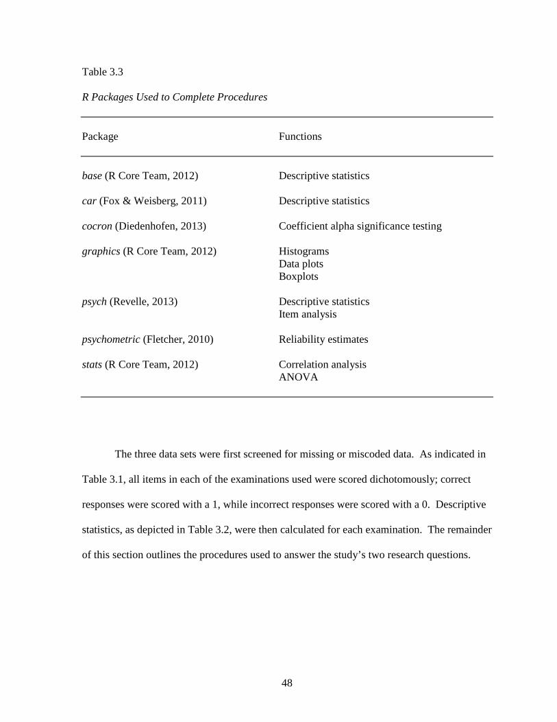
48
Table 3.3 R Packages Used to Complete Procedures Package Functions base (R Core Team, 2012) Descriptive statistics car (Fox & Weisberg, 2011) Descriptive statistics cocron (Diedenhofen, 2013) Coefficient alpha significance testing graphics (R Core Team, 2012) Histograms Data plots Boxplots psych (Revelle, 2013) Descriptive statistics Item analysis psychometric (Fletcher, 2010) Reliability estimates stats (R Core Team, 2012) Correlation analysis ANOVA
The three data sets were first screened for missing or miscoded data. As indicated in
Table 3.1, all items in each of the examinations used were scored dichotomously; correct
responses were scored with a 1, while incorrect responses were scored with a 0. Descriptive
statistics, as depicted in Table 3.2, were then calculated for each examination. The remainder
of this section outlines the procedures used to answer the study’s two research questions.

49
Research Question 1
The first research question addressed the degree to which item discrimination values
are affected when those values are calculated using scores from samples of examinees within
ability ranges around real or anticipated cut scores. To begin, unrestricted discrimination
values – those calculated in a traditional manner using all examinee responses available –
were calculated for all examination items. Calculating unrestricted discrimination values was
necessary, as these values served as a baseline against which the restricted values were
subsequently compared.
The point-biserial statistic, rpbis, was used to estimate item discrimination throughout
this study. As described previously, the point-biserial is calculated as follows:
rpbis=µ +−µx
σ x
p−q (3.1)
where µ+ is the mean total score for those who respond to the item correctly;
µx is the mean total score for the total group of examinees;
σx is the standard deviation for the total group of examinees;
p is the item’s difficulty index; and
q is equal to (1 - p) (Crocker & Algina, 2008).
The point-biserial correlation, which is the observed correlation between item
performance and test performance, was selected because it is one of the most commonly used
estimates of item discrimination, thus facilitating replications of the procedures used in this
study. In addition, previously described research (Oosterhof, 1976; Beuchert & Mendoza,
1979) found differences between estimates produced by the various discrimination indices to

50
be insignificant. Use of the point-biserial, as opposed to any other discrimination statistic,
therefore, was deemed to have not affected the outcome of the study.
Next, the actual examination cut score, CX1, was used as a center point for several
groups of test scores upon which restricted point-biserial statistics were subsequently
calculated. The actual cut score is defined as the score the examination’s governing body or
agency approved as the minimum score required in order to pass the test. The restricted
point-biserials were calculated in the same manner as the unrestricted values, but were based
on fewer test scores. Each group of test scores was centered on the original cut score, but
varied in size according to the following increments:
• Original cut score ± 1.00 SD
• Original cut score ± .75 SD
• Original cut score ± .50 SD
Thus, the three groups of test scores upon which the restricted point-biserials were calculated
varied in size according to distance from the original cut score. The largest group included
all examinee scores within 1.00 SD of the original cut score. The next largest group included
those within .75 SD of the original cut score. The smallest group included only those scores
within .50 SD of the original cut score.
Focusing on smaller groups of test scores around the examination cut score allowed
for an increased focus on that portion of the distribution of scores for which classification
accuracy is most important. According to Clauser et al. (2006), classification accuracy is the
central issue of validity theory with regards to credentialing examinations. Likewise, the
Standards (AREA et al., 1999) call for precision “in the vicinity of the passing, or cut, score”
(p. 157). It seems important, therefore, to clarify the degree to which test items discriminate
51
among those examinees who obtain scores near the examination cut score. It was also
important to assess how the size of the group of test scores considered affected the item
discrimination values. By calculating restricted discrimination indices for the three groups of
test scores described earlier, this analysis was made possible.
The process described thus far was repeated at four additional cut score locations.
These locations were set at the actual cut score plus 1 SEM (CX2) and minus 1 SEM (CX3),
and the actual cut score plus 2 SEM (CX4) and minus 2 SEM (CX5). These new cut score
locations then also served as central points around which item discrimination values for three
groups of test scores were calculated: scores ± 1.00 SD, scores ± .75 SD, and scores ± .50
SD. Calculating discrimination values at these four additional cut score locations was
important because in many instances the cut scores recommended by the results of a standard
setting procedure vary from year to year. Adjustments to examination cut scores are not
uncommon, and may be due to changes in the examination itself, or the composition of the
standard setting panel.
When discrimination values are calculated using limited groups of examinee test
scores around cut scores, the cut score represents a unique location in the distribution of all
test scores. A change in the location of cut score represents a different point in that
distribution. It is helpful to assess, therefore, the degree to which the location of the cut score
affects item discrimination values when those values are calculated using limited samples of
examinee test scores. Using the actual cut score, as well as the actual cut score, plus and
minus 1 and 2 SEM, as central points around which groups of scores are used to calculate
discrimination values helped to determine how changes in the location of the cut score
affected those values.

52
The procedures used to answer Research Question 1 resulted in the calculation of 16
unique discrimination values for each examination item: 1 unrestricted point-biserial
calculated using all available test scores, and 15 restricted point-biserial calculated using
three groups of test scores around each of the five cut scores. The location and size of the
groups upon which the 15 restricted values were calculated are depicted in Table 3.4
After the 15 sets of restricted point-biserials were calculated for each examination
item, the values were compared to their corresponding unrestricted point-biserials. The
initial analysis of differences between the restricted and unrestricted values was based on
visual comparisons. Each set of restricted values was jointly plotted with the corresponding
unrestricted values, allowing for a better understanding of differences and general trends.
Next, a series of boxplots were produced. Each boxplot represented one of the 15 conditions
under which the restricted point-biserials were calculated. These boxplots were displayed
alongside a boxplot representing the unrestricted values. The procedure allowed for a visual
comparison of means and the variation of values between the 15 sets of restricted point-
biserials and the unrestricted set.
Actual differences between the restricted and unrestricted values were also calculated.
For each condition, the item-level differences were characterized with regard to their
direction and magnitude. The mean item discrimination value for the examination was also
calculated for each condition. These mean values were then compared to the mean value of
the unrestricted point-biserials. These procedures provided further insights into general
trends regarding changes in magnitude and direction of the item discrimination values as the
conditions were applied.

53
Table 3.4.
Description of Item Discrimination Values Calculated Cut score Cut score location Size of group used to calculate point-biserial CX1 Actual cut score CX1 ± 1.00 SD CX1 ± .75 SD CX1 ± .50 SD CX2 CX1 + 1 SEM CX2 ± 1.00 SD CX2 ± .75 SD CX2 ± .50 SD CX3 CX1 – 1 SEM CX3 ± 1.00 SD CX3 ± .75 SD CX3 ± .50 SD CX4 CX1 + 2 SEM CX4 ± 1.00 SD CX4 ± .75 SD CX4 ± .50 SD CX5 CX1 – 2 SEM CX5 ± 1.00 SD CX5 ± .75 SD CX5 ± .50 SD Note. Point-biserial statistics were used to estimate item discrimination values.
The procedures described thus far helped to establish a broader understanding of how
limiting examinee scores upon which discrimination values are calculated to those within a
specified distance of an examination cut score affects those values. To examine the degree to
which the differences between restricted an unrestricted values were or were not statistically
significant, however, two addition procedures were conducted. First, a correlation analysis
of the 16 sets of point-biserials was conducted. The correlation coefficients generated were
tested for statistical significance at the α = .05 level. A correlation matrix was produced and

54
is included in the results. The correlation analysis helped to determine where the
relationships between the sets of point-biserials were strongest and weakest. This was
important as it helped to identify those conditions that resulted in the greatest differences
between restricted and unrestricted values.
Next, in order to ascertain the presence of statistically significant differences among
the sets of point-biserials, a one-way analysis of variance (ANOVA) procedure was
conducted. ANOVA procedures are used to test for differences among the means of two or
more samples (Huck, 2008). In this study, item discrimination value was the dependent
variable and the conditions under which the values were calculated served as the independent
variables. The analysis was used to test for differences among the means of the 15 sets of
restricted point-biserials and the unrestricted set. The null hypothesis tested, therefore, was:
H0: µ1 = µ2 = µ3 = µ4 = ... µ16
Four assumptions are associated with ANOVA procedures. These include
independence, randomness, normality, and homogeneity of variance (Huck, 2008). Because
the procedure involved the analysis of the same sets of items under various conditions, the
assumption of independence could not be assumed. As a result, a one-way repeated
measures ANOVA technique was used to analyze the data. Repeated measures ANOVAs are
frequently used when participants or other entities are measured according to some factor
over repeated occasions (Huck, 2008).
The purpose of ANOVA using repeated measures is identical to that of those without
repeated measures: to test the null hypothesis that the means among the groups of data are

55
equal. Repeated measures ANOVAs, however, are also subject to the assumption of
sphericity. This assumption is satisfied when the population variances, as well as all of the
bivariate correlations, are identical (Huck, 2008). When the assumption is not met, the F-
value produced by the ANOVA will be too large. Mauchly’s (1940) test, a procedure
frequently used to assess sphericity, was used in this study to evaluate compliance with this
assumption. The null hypothesis for the Mauchly test is that the differences in variances
between the groups from which the samples were drawn are all equal. This null hypothesis
can be expressed in the following terms:
H0 :σ y1−y2
2 =σ y1−y3
2 =σ y2−y3
2 ...
Violations of the sphericity assumption were corrected using an approach developed
by Greenhouse and Geisser (1959). This Greenhouse-Geisser technique bases the critical F-
value on the degrees of freedom that would have been appropriate if only two levels of the
repeated measure had been used. By doing so, the approach assumes maximum violation of
the sphericity assumption, and produces a conservative F statistic (Huck, 2008). Finally,
analysis of differences was conducted using Tukey’s honest significant difference (HSD)
test. All of the procedures associated with the repeated measures ANOVA used in this study
were tested at the α = .05 level of significance.
In sum, then, the procedures used to characterize the differences between the
unrestricted point-biserials and the restricted values included visual comparisons, analysis of
differences in discrimination values at the individual item and examination levels, a

56
correlation analysis, and ANOVA procedures. Collectively, these procedures led to a better
understanding of Research Question 1.
Research Question 2
The second research question addressed the degree to which restricted item
discrimination values affects certain key test specifications, including item selection,
examination reliability, and classification decision consistency. This section outlines the
procedures followed to answer this question.
In order to evaluate how restricted point-biserials affect the aforementioned
psychometric aspects of credentialing examinations, each examination used in this study was
treated as a test bank from which items were drawn to create two forms of a new 50-item
examination. The bank’s 50 most discriminating items, as determined by the items’
unrestricted point-biserial values, were used to create a pseudo form, Form A. A second
pseudo form, Form B, was also created, comprised of the bank’s 50 most discriminating
items as determined by the items’ restricted point-biserial values. The restricted point-
biserials used to select items for Form A were based on examinee scores within 1.00 SD of
the actual examination cut score (CX1). The forms were created for each of the examinations
used in this study.
After the two forms were created, item selection consistency across the forms was
evaluated. Because the criteria by which items were selected for the two forms were
different – Form A utilized unrestricted discrimination values and Form B utilized restricted
values – it was anticipated that they would likely include different items. Any observed
differences in items between the two forms would indicate that the use of restricted point-

57
biserials resulted in the selection of items that were different than those selected using
unrestricted, or traditionally calculated, point-biserials.
Form A and Form B were also used to measure how restricted item discrimination
values affected examination reliability. The estimate of examination reliability used in this
study was coefficient alpha (Cronbach, 1951). Coefficient alpha was selected because it is a
versatile and widely used measure of examination reliability, which requires, unlike other
reliability estimates, only a single test administration. Coefficient alpha was calculated for
the test variants using the following equation:
(3.2)
where k is the number of items on the examination;
is the variance of item i; and
is the total test variance (Crocker & Algina, 2008).
The coefficients were tested for significant differences at the α = .05 level of
significance using the cocron package (Diedenhofen, 2013) in R (R Core Team, 2012). The
package incorporates earlier work by Alsawalmeh and Feldt (1994) who developed a model
by which the null hypothesis of equal coefficient alphas among dependent samples can be
tested. This null hypothesis can be stated in the following terms:
H0 = α1 – α2 = 0
α̂ =k
k−11−
Σσ̂ i2
σ̂ x2
σ̂ i2
σ̂ x2

58
Alsawalmeh and Feldt’s model can be expressed in the following terms:
W &~1−α̂ 2
1−α̂1(Fv, v), v=
N −1− 7r1,22
1− r1,22
(3.3)
where α1 and α2 are the coefficient alpha values for the examinations; and
r1,22 is the squared correlation coefficient between the examination total scores.
It is important to note, however, that the reliability estimates for both forms were
calculated using all examinee test scores. Although the items selected for Form B were those
that were most discriminating among examinees with total scores within 1.00 SD of the
original cut score only, using this subset of scores to calculate examination reliability for
Form B would have resulted in it being less reliable than Form A in all cases. This is
because the number of cases, or N size, directly affects reliability, with, all other things being
equal, examinations with more cases generally producing larger reliability coefficients than
examinations with fewer cases (Crocker & Algina, 2008). The selection of items for Form B
was based on a substantially smaller number of cases. Because those cases were all within
1.00 SD of the cut score, they were also much more homogenous than the group of scores
used to select items for Form A (i.e. all cases). The homogeneity of a group of examinees is
an important factor that affects the magnitude of reliability estimates. In general, higher
levels of group homogeneity result in lower estimates of reliability because in such
situations, total test variance is diminished (Crocker & Algina, 2008). As documented in
Equation 3.2, total test variance is an element in the calculation of coefficient alpha. It was
necessary to base all estimates of reliability, therefore, on all test scores available. In

59
summary, then, although the items found on Form A and Form B were selected using
divergent methods for calculating item discrimination, estimates of reliability for both forms
were based on all test scores available.
Similar procedures were used to measure the degree to which using restricted item
discrimination values as the item selection criterion affected examination classification
decision consistency. In this study, Cohen’s (1960) κ was used to estimate classification
decision consistency. As described in Chapter 2, the coefficient can be calculated using the
following formula:
(3.4)
where Pc, also referred to as the chance consistency, is the probability of a consistent
decision, and may be calculated using the following formula:
(3.5)
where P1. represents the probability of a mastery classification on one form of an
examination;
P.1 represents a similar probability on the another equivalent form; and
P0. and P.0, which represent misclassifications on the forms.
Coefficient represents the increase in decision consistency over that expected by chance.
The coefficient is equal to 0.00 when there is no increase, and 1.00 when there is maximum
increase (Crocker & Algina, 2008).
κ =P−Pc
1−Pc
Pc = P1.P.1= P0.P.0
κ
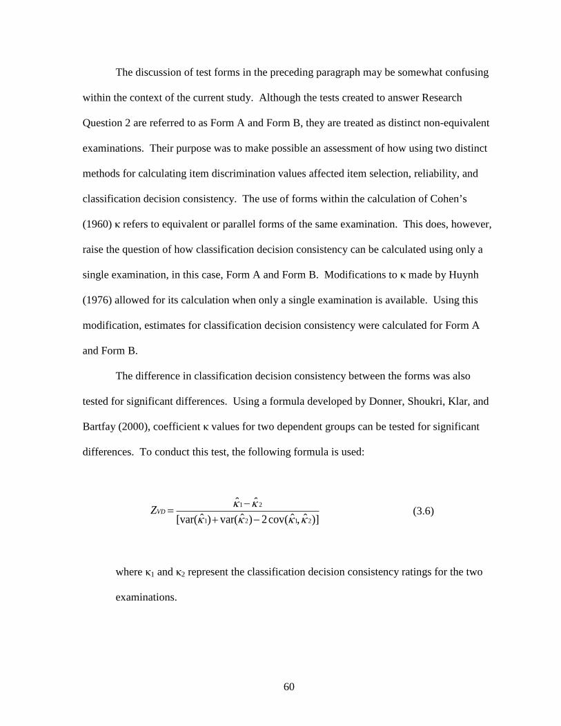
60
The discussion of test forms in the preceding paragraph may be somewhat confusing
within the context of the current study. Although the tests created to answer Research
Question 2 are referred to as Form A and Form B, they are treated as distinct non-equivalent
examinations. Their purpose was to make possible an assessment of how using two distinct
methods for calculating item discrimination values affected item selection, reliability, and
classification decision consistency. The use of forms within the calculation of Cohen’s
(1960) κ refers to equivalent or parallel forms of the same examination. This does, however,
raise the question of how classification decision consistency can be calculated using only a
single examination, in this case, Form A and Form B. Modifications to κ made by Huynh
(1976) allowed for its calculation when only a single examination is available. Using this
modification, estimates for classification decision consistency were calculated for Form A
and Form B.
The difference in classification decision consistency between the forms was also
tested for significant differences. Using a formula developed by Donner, Shoukri, Klar, and
Bartfay (2000), coefficient κ values for two dependent groups can be tested for significant
differences. To conduct this test, the following formula is used:
(3.6)
where κ1 and κ2 represent the classification decision consistency ratings for the two
examinations.
ZVD =κ̂1− κ̂ 2
[var(κ̂1)+ var(κ̂ 2)−2cov(κ̂1,κ̂ 2)]

61
The formula tests the null hypothesis that the difference between the coefficients is zero:
H0 = κ1 - κ2 = 0
The test for differences between κ coefficients was also tested at the α = .05 level of
significance.
The procedures described in this section were used to answer Research Question 2.
That is, they led to a determination of the degree to which using restricted item
discrimination values as a criterion for selecting examination items affected item selection,
examination reliability, and classification decision consistency. The procedures were
conducted for each of the three examination used in this study. By doing so, greater insight
into the role sample size plays in these considerations was possible.
The three variables examined in Research Question 2, namely item selection,
examination reliability, and classification decision consistency, are critical elements in the
gathering of validity evidence for credentialing examinations. Understanding how
examinations with items that were selected using restricted discrimination values affects
these specifications, therefore, becomes a valuable endeavor. Again, according to the
Standards (AERA et al., 1999), examinations used for credentialing individuals “may not
need to be precise for those who clearly pass or clearly fail,” as “sometimes a test used in
credentialing is designed to be precise only in the vicinity of the cut score” (p. 157).

62
CHAPTER 4
RESULTS
Utilizing examinee scores from three examinations used to credential individuals in
health-related professions, the study examined the degree to which limiting scores upon
which item discrimination values are calculated to those near actual or anticipated cut scores
affected the item discrimination values, item selection, examination reliability, and
classification decision consistency. An initial analysis of the data used found that there were
no missing or miscoded responses. Procedures were then followed to answer the study’s two
research questions. Research Question 1 addressed the effect on item discrimination values.
Research Question 2 examined the effect on item selection, examination reliability, and
classification decision consistency. The results for each research question are addressed in
the sections that follow.
Research Question 1
Research Question 1 examined the effect limiting scores upon which item
discrimination values are calculated to those near actual or anticipated cut scores had on item
discrimination values themselves. To accomplish this, the unrestricted point-biserial statistic,
rpbis, was calculated for each examination item. Restricted point-biserials were then
calculated for all items under each of 15 conditions. These conditions, as well as the cut
scores and examinee scores that were considered under each condition, are listed in Table
4.1. Differences between the restricted and unrestricted values were then analyzed. The
results for each examination are presented individually in the sections that follow.

63
Table 4.1
Conditions for the Calculation of Restricted Point-biserials
Stat/Cut Score Group Examination 1 Examination 2 Examination 3 No. Items 175 200 149 SD 19.55 18.23 9.01 SEM 5.79 5.84 4.44 CX1 115 128 106 (Actual CX) +/- 1.00 SD 96 – 134 110 – 146 97 – 115 +/- 0.75 SD 101 – 129 115 – 141 100 – 112 +/- 0.50 SD 106 – 124 119 – 137 102 – 110 CX2 121 134 111 (+ 1 SEM) +/- 1.00 SD 102 – 140 116 – 152 102 – 119 +/- 0.75 SD 107 – 135 121 – 147 104 – 117 +/- 0.50 SD 112 – 130 125 – 142 106 – 114 CX3 110 123 102 (- 1 SEM) +/- 1.00 SD 90 – 128 104 – 140 93 – 110 +/- 0.75 SD 95 – 123 109 – 135 95 – 108 +/- 0.50 SD 100 – 118 114 – 131 98 – 106 CX4 127 140 115 (+ 2 SEM) +/- 1.00 SD 108 – 146 122 – 157 106 – 123 +/- 0.75 SD 112 – 141 127 – 153 109 – 121 +/- 0.50 SD 117 – 136 131 - 148 111 – 119 CX5 104 117 98 (- 2 SEM) +/- 1.00 SD 84 – 122 99 – 134 89 – 106 +/- 0.75 SD 89 – 118 103 – 129 91 – 103 +/- 0.50 SD 94 – 113 108 – 125 93 – 101 Note. Ranges indicate examinee scores considered in the calculation of item discrimination values at each cut score location.

64
Examination 1
Examination 1, which in terms of sample size was the largest test used in the study,
consisted of 490 examinee responses to 175 items. The initial analyses of differences
between restricted and unrestricted discrimination values were based on visual comparisons.
First, the unrestricted and restricted discrimination values for each of the five cut scores used
were plotted. Figure 4.1 displays the unrestricted values plotted along side the restricted
values calculated using scores within 1.00 SD, .75 SD, and .50 SD of CX1 (the actual cut
score). Figures 4.2, 4.3, 4.4, and 4.5 show the same information for CX2, CX3, CX4, and CX5,
respectively.
The plots displayed in Figures 4.1 through 4.5 suggest that unrestricted item
discrimination values are, in general, larger than their corresponding restricted values. This
appeared to be the case at each of the five cut score locations examined. As the size of the
groups of test scores used to calculate the restricted discrimination values became smaller,
the discrimination values themselves were generally smaller. For example, item
discrimination values calculated using only scores within .50 SD of the cut scores appeared
to be smaller than values calculated using scores within .75 SD and 1.00 SD of the cut scores.
To further understand general trends associated with the differences in the
discrimination values calculated, a boxplot was also produced. As seen in Figure 4.6, the
distribution of unrestricted point-biserials included larger discrimination values than any
other group of values. As suggested by the plots in Figures 4.1 through 4.5, the boxplot also
indicates that the values decrease as the size of the group used to calculate them becomes
smaller.

Unrestricted 1.00 SD 0.75 SD 0.50 SD
Figure 4.1. Plots of unrestricted and restricted item discrimination values based on scores within 1.00 SD, 0.75 SD, and 0.50 SD of CX1 for Examination 1.
0 50 100 150
Examination Items
0 50 100 150
Examination Items
0 50 100 150
Examination Items
0 50 100 150
-0.5
0.0
0.5
1.0
Examination Items
Poi
nt-b
iser
ial V
alue
65
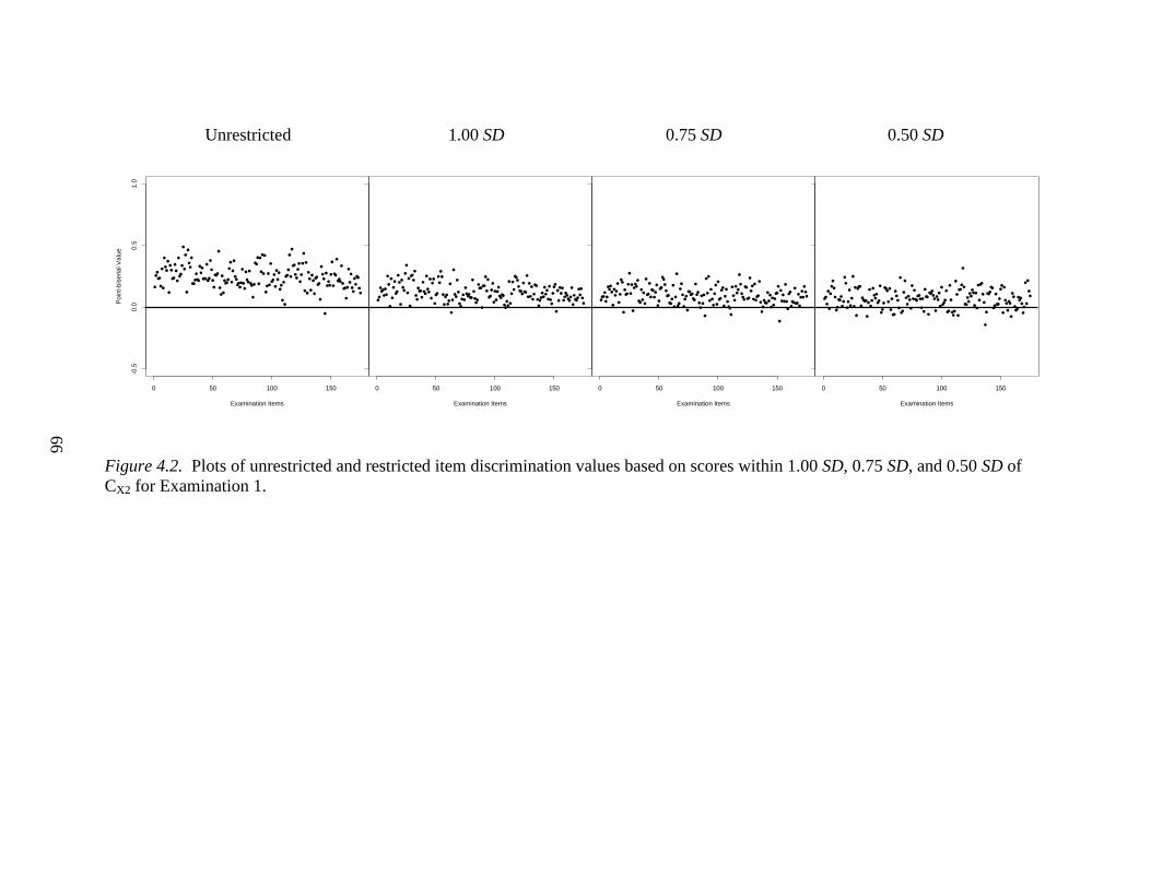
Unrestricted 1.00 SD 0.75 SD 0.50 SD
Figure 4.2. Plots of unrestricted and restricted item discrimination values based on scores within 1.00 SD, 0.75 SD, and 0.50 SD of CX2 for Examination 1.
0 50 100 150
-0.5
0.0
0.5
1.0
Examination Items
Poi
nt-b
iser
ial V
alue
0 50 100 150
Examination Items
0 50 100 150
Examination Items
0 50 100 150
Examination Items
66
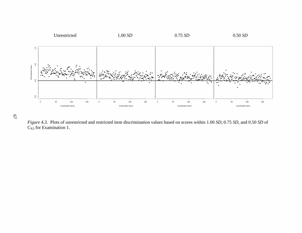
Unrestricted 1.00 SD 0.75 SD 0.50 SD
Figure 4.3. Plots of unrestricted and restricted item discrimination values based on scores within 1.00 SD, 0.75 SD, and 0.50 SD of CX3 for Examination 1.
0 50 100 150
-0.5
0.0
0.5
1.0
Examination Items
Poi
nt-b
iser
ial V
alue
0 50 100 150
Examination Items
0 50 100 150
Examination Items
0 50 100 150
Examination Items
67

Unrestricted 1.00 SD 0.75 SD 0.50 SD
Figure 4.4. Plots of unrestricted and restricted item discrimination values based on scores within 1.00 SD, 0.75 SD, and 0.50 SD of CX4 for Examination 1.
0 50 100 150
-0.5
0.0
0.5
1.0
Examination Items
Poi
nt-b
iser
ial V
alue
0 50 100 150
Examination Items
0 50 100 150
Examination Items
0 50 100 150
Examination Items
68

Unrestricted 1.00 SD 0.75 SD 0.50 SD
Figure 4.5. Plots of unrestricted and restricted item discrimination values based on scores within 1.00 SD, 0.75 SD, and 0.50 SD of CX5 for Examination 1.
0 50 100 150
-0.5
0.0
0.5
1.0
Examination Items
Poi
nt-b
iser
ial V
alue
0 50 100 150
Examination Items
0 50 100 150
Examination Items
0 50 100 150
Examination Items
69
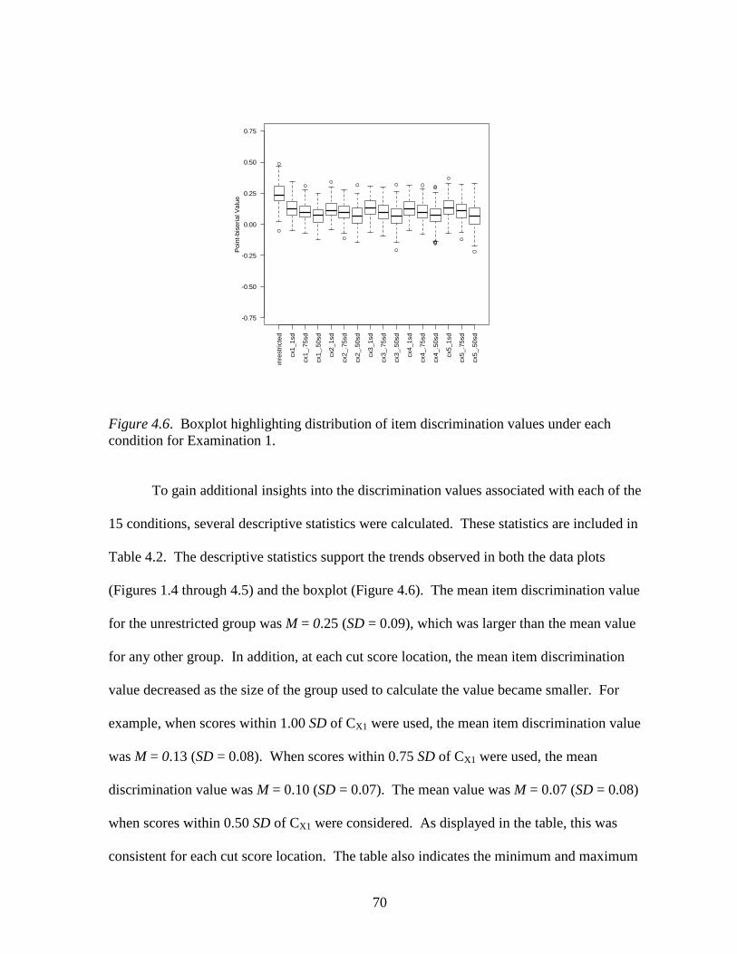
70
Figure 4.6. Boxplot highlighting distribution of item discrimination values under each condition for Examination 1.
To gain additional insights into the discrimination values associated with each of the
15 conditions, several descriptive statistics were calculated. These statistics are included in
Table 4.2. The descriptive statistics support the trends observed in both the data plots
(Figures 1.4 through 4.5) and the boxplot (Figure 4.6). The mean item discrimination value
for the unrestricted group was M = 0.25 (SD = 0.09), which was larger than the mean value
for any other group. In addition, at each cut score location, the mean item discrimination
value decreased as the size of the group used to calculate the value became smaller. For
example, when scores within 1.00 SD of CX1 were used, the mean item discrimination value
was M = 0.13 (SD = 0.08). When scores within 0.75 SD of CX1 were used, the mean
discrimination value was M = 0.10 (SD = 0.07). The mean value was M = 0.07 (SD = 0.08)
when scores within 0.50 SD of CX1 were considered. As displayed in the table, this was
consistent for each cut score location. The table also indicates the minimum and maximum
unre
stric
ted
cx1_
1sd
cx1_
.75s
d
cx1_
.50s
d
cx2_
1sd
cx2_
.75s
d
cx2_
.50s
d
cx3_
1sd
cx3_
.75s
d
cx3_
.50s
d
cx4_
1sd
cx4_
.75s
d
cx4_
.50s
d
cx5_
1sd
cx5_
.75s
d
cx5_
.50s
d
-0.75
-0.50
-0.25
0.00
0.25
0.50
0.75
Poi
nt-b
iser
ial V
alue

71
value for each condition, as well as the range of values. In addition, it includes the number
of test scores that were considered for each of the conditions examined. The set of restricted
values that included the most examinee scores was that which considered scores within 1.00
SD of CX3. Calculations for this set included 344 scores. The set with the fewest scores
included those within 0.50 SD of CX5. For this set, only 152 test scores were used to
calculate the point-biserials.
To further understand the nature of the relationships between the sets of
discrimination values, a correlation table was produced. The correlation table is included in
Table 4.3. As seen in the table, 102 of the 120 correlation coefficients calculated were
significantly different than zero at the α = .05 level of significance. Of particular interest
were the relationships between the unrestricted discrimination values and each of the 15
restricted sets of values. In each case, the correlation coefficient between these sets of values
was found to be significantly different than zero. The strongest correlation observed was
between discrimination values calculated using examinee scores within 1.00 SD of CX1 and
values calculated using scores between 0.75 SD of CX1, r(173) = .84, p < .001. The weakest
correlation, .02, was found between four sets of values. In each of these instances, the
correlation was found to be not significantly different than zero. The majority of correlation
coefficients expressed positive relationships between the sets of values, with only 12 of the
120 coefficients expressing negative relationships.

72
Table 4.2
Descriptive Statistics of Discrimination Values Calculated for Examination 1
Cut Score Group M SD Min Max Range Skew n Unrestricted
0.25
0.09
-0.05
0.49
0.54
0.11
490
CX1 +/- 1.00 SD
0.13 0.08 -0.05 0.35 0.40 0.35 339
+/- 0.75 SD
0.10 0.07 -0.07 0.31 0.38 0.33 287
+/- 0.50 SD
0.07 0.08 -0.12 0.25 0.37 0.14 198
CX2 +/- 1.00 SD
0.12 0.07 -0.04 0.34 0.38 0.37 317
+/- 0.75 SD
0.10 0.07 -0.11 0.27 0.39 0.03 267
+/- 0.50 SD
0.07 0.08 -0.14 0.32 0.46 0.12 200
CX3 +/- 1.00 SD
0.14 0.08 -0.06 0.31 0.37 0.11 344
+/- 0.75 SD
0.10 0.08 -0.10 0.30 0.40 0.02 255
+/- 0.50 SD
0.07 0.09 -0.21 0.32 0.53 -0.05 171
CX4 +/- 1.00 SD
0.13 0.07 -0.05 0.31 0.36 0.17 292
+/- 0.75 SD
0.10 0.08 -0.08 0.31 0.39 0.22 240
+/- 0.50 SD
0.07 0.09 -0.15 0.30 0.45 -0.13 169
CX5 +/- 1.00 SD
0.14 0.08 -0.07 0.37 0.44 0.13 307
+/- 0.75 SD
0.11 0.08 -0.12 0.32 0.44 0.06 239
+/- 0.50 SD 0.07 0.10 -0.22 0.33 0.55 -0.11 152

Table 4.3
Correlation Matrix of Item Discrimination Values Calculated for Examination 1
CX1 CX2 CX3 CX4 CX5 UNR 1.00 SD 0.75 SD 0.50 SD 1.00 SD 0.75 SD 0.50 SD 1.00 SD 0.75 SD 0.50 SD 1.00 SD 0.75 SD 0.50 SD 1.00 SD 0.75 SD 0.50 SD
UNR 1.00
CX1 1.00 SD 0.76* 1.00 0.75 SD 0.67* 0.84* 1.00 0.50 SD 0.41* 0.45* 0.59* 1.00
CX2
1.00 SD 0.68* 0.83* 0.83* 0.55* 1.00 0.75 SD 0.53* 0.69* 0.67* 0.60* 0.82* 1.00 0.50 SD 0.34* 0.54* 0.55* 0.27* 0.59* 0.69* 1.00
CX3
1.00 SD 0.79* 0.82* 0.76* 0.42* 0.64* 0.48* 0.38* 1.00 0.75 SD 0.67* 0.76* 0.64* 0.48* 0.50* 0.27* 0.07 0.78* 1.00 0.50 SD 0.45* 0.50* 0.53* 0.22* 0.34* 0.02 -0.24* 0.53* 0.68* 1.00
CX4
1.00 SD 0.60* 0.68* 0.65* 0.47* 0.84* 0.81* 0.59* 0.46* 0.34* 0.14 1.00 0.75 SD 0.50* 0.61* 0.49* 0.21* 0.79* 0.74* 0.76* 0.39* 0.15* -0.08 0.81* 1.00 0.50 SD 0.34* 0.44* 0.22* -0.16* 0.48* 0.54* 0.42* 0.19* -0.07 -0.08 0.48* 0.63* 1.00
CX5
1.00 SD 0.79* 0.62* 0.54* 0.38* 0.43* 0.26* 0.05 0.81* 0.81* 0.61* 0.30* 0.15* -0.02 1.00 0.75 SD 0.62* 0.50* 0.33* 0.07 0.23* 0.02 -0.10 0.76* 0.66* 0.65* 0.08 0.02 0.05 0.82* 1.00 0.50 SD 0.34* 0.42* 0.12 -0.25* 0.06 -0.17* -0.17* 0.47* 0.56* 0.43* -0.06 -0.02 0.20* 0.46* 0.62* 1.00 Note. * p = < .05.
73

74
The final procedure performed for each examination with respect to Research
Question 1 was the one-way, repeated measures ANOVA. This was used to test for
differences among the means of the unrestricted discrimination values and the 15 sets of
restricted values. In the ANOVA conducted, the discrimination values served as the
dependent variable and the conditions under which those values were calculated served as the
independent variables, or groups. The purpose of the analysis was to test the null hypothesis
that the group mean discrimination values were equal.
The analysis began with an evaluation of ANOVA assumptions. The discrimination
values, which served as the dependent variable, were not independent. Each group in the
ANOVA consisted of the same subjects, or in this case, examination items, tested under
different conditions. Because of this, a repeated measures ANOVA approach was taken.
Normality was assessed using two procedures. First, the Shapiro-Wilk normality test (R
Core Team, 2012) was performed. The procedure tests the null hypothesis that the data are
normally distributed. The results indicated that all but one of the sets of data was normally
distributed. The set for which the null hypothesis was rejected included values calculated
using scores within 1.00 SD of CX1, W = 0.98, p = .04. Assessing skewness values was the
second test for normality. As seen in Table 4.2, the skewness value for each of the sets of
data fell between -1.00 and 1.00. According to Huck (2008), skewness values that fall within
this range are typically considered to approximate a normal distribution. Based on this
criterion, the data were deemed to have sufficiently satisfied the assumption of normality.
Because the procedure involved a repeated measures approach, the data also needed
to satisfy the assumption of sphericity. In a traditional ANOVA procedure, that is, one that
does not involve repeated measures, sphericity is not required, but rather the assumption of

75
homogeneity of variance is tested. Sphericity is satisfied when the variances and bivariate
correlations among the sets of data are equal (Huck, 2008). This assumption was tested
using Mauchly’s (1940) procedure, which tests the hull hypothesis that the variances and
bivariate correlations among the groups are equal. The results of Mauchly’s test, W < .001, p
< .001, indicated that the assumption of sphericity was not met. When the assumption is not
met, the F-statistic will be positively biased and, therefore, the risk of Type I error increases.
The Greenhouse-Geisser (1959) correction, estimated to be ε = 0.28, was applied to the
degrees of freedom in order to obtain a valid critical F-value. The results of the ANOVA, to
include the Greenhouse-Geisser correction for sphericity, are included in Table 4.4.
Table 4.4
Results of the One-way Repeated Measures ANOVA for Examination 1
Source Model SS df MS F p Condition Sphericity Assumed 5.265 15.000 0.351 94.539 < .001* Greenhouse-Geisser
Corrected 5.265 4.200 1.254 94.539 < .001*
Error Sphericity Assumed 9.690 2610.000 0.004 Greenhouse-Geisser
Corrected 9.690 730.800 0.013
Note. The Greenhouse-Geisser correction, estimated at ε = 0.28, was used to correct for the violation of the sphericity assumption. * = Significant at α = .05 level of significance.

76
As observed in Table 4.4, the results of the corrected ANOVA indicated that
differences between the sets of values were significantly greater than zero, F(4.2, 730.8) =
94.539, p < .001. As such, the null hypothesis of equal means among the groups of
discrimination values was rejected. To assess where differences existed, Tukey’s honest
significant difference (HSD) test was conducted. Although Tukey’s HSD was utilized to
identify significant differences among all groups, the primary objective was to identify
differences between each of the restricted groups and the unrestricted group. The results of
this analysis are included in Table 4.5. As seen in Table 4.5, a significant mean difference
was observed between the unrestricted set of discrimination values and each of the restricted
sets when tested at the α = .05 level of significance. In each instance, the mean unrestricted
value was larger than the mean restricted value.

77
Table 4.5. Results of Tukey’s HSD Test for Examination 1 - Unrestricted vs. Restricted Values Condition Condition Mean difference p Cut score Group size Unrestricted CX1 +/- 1.00 SD 0.119 < .001* +/- 0.75 SD 0.143 < .001* +/- 0.50 SD 0.177 < .001* CX2 +/- 1.00 SD 0.123 < .001* +/- 0.75 SD 0.149 < .001* +/- 0.50 SD 0.177 < .001* CX3 +/- 1.00 SD 0.101 < .001* +/- 0.75 SD 0.149 < .001* +/- 0.50 SD 0.182 < .001* CX4 +/- 1.00 SD 0.120 < .001* +/- 0.75 SD 0.148 < .001* +/- 0.50 SD 0.178 < .001* CX5 +/- 1.00 SD 0.113 < .001* +/- 0.75 SD 0.140 < .001* +/- 0.50 SD 0.180 < .001* Note. * = Significant at the α = .05 level of significance.

78
Examination 2
Examination 2, according to sample size, was the second largest test used in the
study. Responses from 161 examinees to the 200-item examination were included in the
analysis. The procedures conducted with respect to Examination 1 were also performed for
Examination 2. In Figures 4.7 through 4.11, the unrestricted discrimination values are
plotted with their corresponding restricted point-biserials for each of the five cut score
locations. As was the case with Examination 1, the plots revealed that the unrestricted
discrimination values were, in general, larger than the restricted values. The differences
between the restricted and unrestricted values, however, appeared to be, at least visually, less
stark than was the case with the differences observed in Examination 1. Results of the
boxplot, included in Figure 4.12, also suggested that the unrestricted values were larger than
the restricted values. In addition, at each cut score location, the mean discrimination value
decreased in magnitude as the group of scores used to calculate the values grew smaller in
size.
Descriptive statistics for the sets of discrimination values are included in Table 4.6.
As seen in the table, the largest mean discrimination value was associated with the
unrestricted set, M = 0.22 (SD = 0.12). As was the case with Examination 1, the mean
discrimination value decreased as the size of the group of scores considered decreased in
size. The smallest mean discrimination value observed was associated with the set of values
calculated using scores within 0.50 SD of CX5, M = 0.05 (SD = 0.18). This set included 37
examinee scores, which was fewer than for any other set. Values calculated using scores
within 1.00 SD of CX2 considered 115 scores, which was more than any other set of restricted
values.

Unrestricted 1.00 SD 0.75 SD 0.50 SD
Figure 4.7. Plots of unrestricted and restricted item discrimination values based on scores within 1.00 SD, 0.75 SD, and 0.50 SD of CX1 for Examination 2.
0 50 100 150 200
-0.5
0.0
0.5
1.0
Examination Items
Poi
nt-b
iser
ial V
alue
0 50 100 150 200
Examination Items
0 50 100 150 200
Examination Items
0 50 100 150 200
Examination Items
79
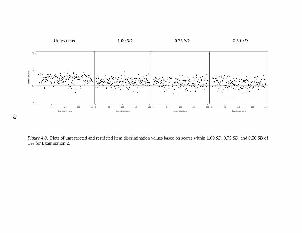
Unrestricted 1.00 SD 0.75 SD 0.50 SD
Figure 4.8. Plots of unrestricted and restricted item discrimination values based on scores within 1.00 SD, 0.75 SD, and 0.50 SD of CX2 for Examination 2.
0 50 100 150 200
-0.5
0.0
0.5
1.0
Examination Items
Poi
nt-b
iser
ial V
alue
0 50 100 150 200
Examination Items
0 50 100 150 200
Examination Items
0 50 100 150 200
Examination Items
80

Unrestricted 1.00 SD 0.75 SD 0.50 SD
Figure 4.9. Plots of unrestricted and restricted item discrimination values based on scores within 1.00 SD, 0.75 SD, and 0.50 SD of CX3 for Examination 2.
0 50 100 150 200
-0.5
0.0
0.5
1.0
Examination Items
Poi
nt-b
iser
ial V
alue
0 50 100 150 200
Examination Items
0 50 100 150 200
Examination Items
0 50 100 150 200
Examination Items
81

Unrestricted 1.00 SD 0.75 SD 0.50 SD
Figure 4.10. Plots of unrestricted and restricted item discrimination values based on scores within 1.00 SD, 0.75 SD, and 0.50 SD of CX4 for Examination 2.
0 50 100 150 200
-0.5
0.0
0.5
1.0
Examination Items
Poi
nt-b
iser
ial V
alue
0 50 100 150 200
Examination Items
0 50 100 150 200
Examination Items
0 50 100 150 200
Examination Items
82

Unrestricted 1.00 SD 0.75 SD 0.50 SD
Figure 4.11. Plots of unrestricted and restricted item discrimination values based on scores within 1.00 SD, 0.75 SD, and 0.50 SD of CX5 for Examination 2.
0 50 100 150 200
-0.5
0.0
0.5
1.0
Examination Items
Poi
nt-b
iser
ial V
alue
0 50 100 150 200
Examination Items
0 50 100 150 200
Examination Items
0 50 100 150 200
Examination Items
83

84
Figure 4.12. Boxplot highlighting distribution of item discrimination values under each condition for Examination 2.
unre
stric
ted
cx1_
1sd
cx1_
.75s
d
cx1_
.50s
d
cx2_
1sd
cx2_
.75s
d
cx2_
.50s
d
cx3_
1sd
cx3_
.75s
d
cx3_
.50s
d
cx4_
1sd
cx4_
.75s
d
cx4_
.50s
d
cx5_
1sd
cx5_
.75s
d
cx5_
.50s
d
-0.75
-0.50
-0.25
0.00
0.25
0.50
0.75
Poi
nt-b
iser
ial V
alue
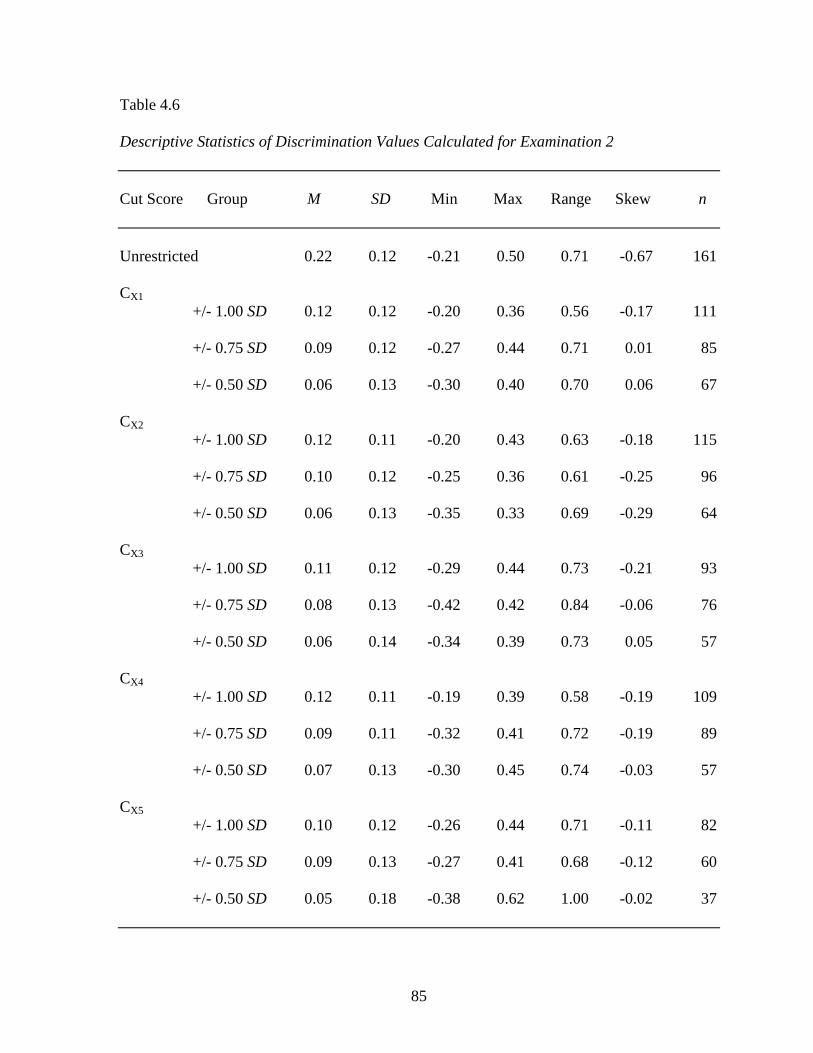
85
Table 4.6
Descriptive Statistics of Discrimination Values Calculated for Examination 2
Cut Score Group M SD Min Max Range Skew n Unrestricted
0.22
0.12
-0.21
0.50
0.71
-0.67
161
CX1 +/- 1.00 SD
0.12 0.12 -0.20 0.36 0.56 -0.17 111
+/- 0.75 SD
0.09 0.12 -0.27 0.44 0.71 0.01 85
+/- 0.50 SD
0.06 0.13 -0.30 0.40 0.70 0.06 67
CX2 +/- 1.00 SD
0.12 0.11 -0.20 0.43 0.63 -0.18 115
+/- 0.75 SD
0.10 0.12 -0.25 0.36 0.61 -0.25 96
+/- 0.50 SD
0.06 0.13 -0.35 0.33 0.69 -0.29 64
CX3 +/- 1.00 SD
0.11 0.12 -0.29 0.44 0.73 -0.21 93
+/- 0.75 SD
0.08 0.13 -0.42 0.42 0.84 -0.06 76
+/- 0.50 SD
0.06 0.14 -0.34 0.39 0.73 0.05 57
CX4 +/- 1.00 SD
0.12 0.11 -0.19 0.39 0.58 -0.19 109
+/- 0.75 SD
0.09 0.11 -0.32 0.41 0.72 -0.19 89
+/- 0.50 SD
0.07 0.13 -0.30 0.45 0.74 -0.03 57
CX5 +/- 1.00 SD
0.10 0.12 -0.26 0.44 0.71 -0.11 82
+/- 0.75 SD
0.09 0.13 -0.27 0.41 0.68 -0.12 60
+/- 0.50 SD 0.05 0.18 -0.38 0.62 1.00 -0.02 37

86
The correlation matrix developed for Examination 2 is included in Table 4.7. Among
the 120 correlation coefficients calculated, 99 were found to be significantly different than
zero at the α = 0.05 level of significance. The strongest correlation observed was between
values calculated using scores within 1.00 SD of CX2 and values calculated using scores
within 1.00 SD of CX4, r(198) = 0.83, p < .001. The weakest correlation observed was
between values calculated using scores within 0.75 SD of CX2 and values calculated using
scores within 0.75 SD of CX5. The correlation between these sets of values was not
significantly different than zero. The majority of coefficients were positive, with only 24 of
the 120 expressing negative relationships.
One-way repeated measures ANOVA was also conducted for the sets of
discrimination values associated with Examination 2. Tests for normality were similar to
those conducted for Examination 1. The Shapiro-Wilk normality test (R Core Team, 2012)
results indicated that the assumption of normality was not satisfied for one of the sets of
values. The null hypothesis of normality was rejected for the set of unrestricted
discrimination values, W = 0.97, p < .001. As seen in Table 4.6, however, the skewness
values for each set of point-biserials ranged between -1.00 and 1.00, indicating the data
approximated normality. The data were, therefore, deemed suitable for further analysis.
Mauchly’s (1940) test indicated that the assumption of sphericity had not been
satisfied, W < 0.001, p < .001. The Greenhouse-Geisser (1959) correction, ε = 0.28, was
once again applied to the degrees of freedom in order to combat the effects associated with
the violation of the sphericity assumption. The results of the ANOVA are included in Table
4.8.

Table 4.7
Correlation Matrix of Item Discrimination Values Calculated for Examination 2
CX1 CX2 CX3 CX4 CX5 UNR 1.00 SD 0.75 SD 0.50 SD 1.00 SD 0.75 SD 0.50 SD 1.00 SD 0.75 SD 0.50 SD 1.00 SD 0.75 SD 0.50 SD 1.00 SD 0.75 SD 0.50 SD
UNR 1.00 CX1
1.00 SD 0.66* 1.00 0.75 SD 0.48* 0.69* 1.00 0.50 SD 0.33* 0.51* 0.70* 1.00 CX2
1.00 SD 0.69* 0.70* 0.61* 0.52* 1.00 0.75 SD 0.56* 0.71* 0.61* 0.51* 0.82* 1.00 0.50 SD 0.36* 0.40* 0.48* 0.12 0.49* 0.59* 1.00 CX3
1.00 SD 0.55* 0.73* 0.69* 0.53* 0.41* 0.37* 0.22* 1.00 0.75 SD 0.43* 0.70* 0.51* 0.51* 0.27* 0.20* -0.09 0.78* 1.00 0.50 SD 0.25* 0.50* 0.53* 0.49* 0.22* 0.14* -0.28* 0.54* 0.70* 1.00 CX4
1.00 SD 0.62* 0.53* 0.40* 0.26* 0.83* 0.78* 0.52* 0.20* 0.06 -0.04* 1.00 0.75 SD 0.54* 0.35* 0.13 -0.11 0.65* 0.52* 0.59* 0.01 -0.18* -0.34* 0.74* 1.00 0.50 SD 0.27* 0.26* -0.14 -0.27* 0.38* 0.42* 0.20* -0.12* -0.18* -0.14* 0.48* 0.59* 1.00 CX5
1.00 SD 0.51* 0.52* 0.44* 0.46* 0.29* 0.17* -0.08 0.77* 0.77* 0.57* 0.06 -0.13 -0.18* 1.00 0.75 SD 0.34* 0.35* 0.13 0.10 0.06 -0.05 -0.25* 0.64* 0.58* 0.46* -0.08 -0.17* 0.11 0.71* 1.00 0.50 SD 0.22* 0.35* -0.03 -0.24* -0.17* -0.23* -0.06 0.40* 0.56* 0.18 -0.21* 0.05 0.06 0.35* 0.49* 1.00 Note. * p = < .05.
87

88
Table 4.8
Results of the One-way Repeated Measures ANOVA for Examination 2
Source Model SS df MS F p Condition Sphericity Assumed 4.571 15.000 0.305 27.046 < .001* Greenhouse-Geisser
Corrected 4.571 4.200 1.088 27.046 < .001*
Error Sphericity Assumed 33.636 2985.000 0.011 Greenhouse-Geisser
Corrected 33.636 835.800 0.040
Note. The Greenhouse-Geisser correction, estimated at ε = 0.28, was used to correct for the violation of the sphericity assumption. * = Significant at α = .05 level of significance.
As seen in the table, the sphericity-corrected ANOVA produced a significant result,
F(4.20, 835.80) = 27.046, p < .001, indicating that differences among the group means
existed. Tukey’s HSD was used to identify those differences. The results of this test are
included in Table 4.9.

89
Table 4.9 Results of Tukey’s HSD Test for Examination 2 - Unrestricted vs. Restricted Values Condition Condition Mean difference p Cut score Group size Unrestricted CX1 +/- 1.00 SD 0.096 < .001* +/- 0.75 SD 0.128 < .001* +/- 0.50 SD 0.153 < .001* CX2 +/- 1.00 SD 0.095 < .001* +/- 0.75 SD 0.116 < .001* +/- 0.50 SD 0.152 < .001* CX3 +/- 1.00 SD 0.108 < .001* +/- 0.75 SD 0.133 < .001* +/- 0.50 SD 0.155 < .001* CX4 +/- 1.00 SD 0.098 < .001* +/- 0.75 SD 0.121 < .001* +/- 0.50 SD 0.148 < .001* CX5 +/- 1.00 SD 0.111 < .001* +/- 0.75 SD 0.130 < .001* +/- 0.50 SD 0.165 < .001* Note. * = Significant at the α = .05 level of significance.
As was the case with Examination 1, significant differences were identified between the
unrestricted set of values and each of the restricted sets. In each instance, the unrestricted
mean discrimination value was greater than the unrestricted mean values.

90
Examination 3
Examination 3, which was the smallest test used in this study, consisted of 149 items.
Responses from 76 examinees were included in the analysis. The same procedures described
for Examination 1 and Examination 2 were conducted for Examination 3. The plots
depicting the location of unrestricted and restricted discrimination values for each cut score
considered are included in Figures 4.13 through 4.17. Unlike the plots highlighting the same
information for Examinations 1 and 2, the plots for Examination 3 indicated no discernable
visual relationship between the unrestricted and restricted point-biserials. The restricted
discrimination values, in particular, appeared to vary greatly when compared to those
observed for the previous examinations.
The boxplot, included in Figure 18, indicated a somewhat more familiar pattern, with
the mean discrimination value for the unrestricted set being larger than the mean values for
the restricted sets. As was the case with the previous examinations, the mean discrimination
value for each set appeared to decrease as the size of the group of scores considered
decreased.
Descriptive statistics for the values calculated are included in Table 4.10. As the
table indicates, the largest mean discrimination value was that associated with the
unrestricted set, M = 0.16 (SD = 0.13). This was the lowest unrestricted mean discrimination
value among all of the examinations considered in the study. The largest mean
discrimination value among the restricted sets represented point-biserials calculated using
scores within 1.00 SD of CX4. This set considered 52 examinee scores, which was more than
any other restricted set. The set with the fewest number of scores included those within 0.50
SD of CX5. Only six scores were included in the calculations for this set.

Unrestricted 1.00 SD 0.75 SD 0.50 SD
Figure 4.13. Plots of unrestricted and restricted item discrimination values based on scores within 1.00 SD, 0.75 SD, and 0.50 SD of CX1 for Examination 3.
0 50 100 150
-1.0
-0.5
0.0
0.5
1.0
Examination Items
Poi
nt-b
iser
ial V
alue
0 50 100 150
Examination Items
0 50 100 150
Examination Items
0 50 100 150
Examination Items
91

Unrestricted 1.00 SD 0.75 SD 0.50 SD
Figure 4.14. Plots of unrestricted and restricted item discrimination values based on scores within 1.00 SD, 0.75 SD, and 0.50 SD of CX2 for Examination 3.
0 50 100 150
-1.0
-0.5
0.0
0.5
1.0
Examination Items
Poi
nt-b
iser
ial V
alue
0 50 100 150
Examination Items
0 50 100 150
Examination Items
0 50 100 150
Examination Items
92

Unrestricted 1.00 SD 0.75 SD 0.50 SD
Figure 4.15. Plots of unrestricted and restricted item discrimination values based on scores within 1.00 SD, 0.75 SD, and 0.50 SD of CX3 for Examination 3.
0 50 100 150
-1.0
-0.5
0.0
0.5
1.0
Examination Items
Poi
nt-b
iser
ial V
alue
0 50 100 150
Examination Items
0 50 100 150
Examination Items
0 50 100 150
Examination Items
93

Unrestricted 1.00 SD 0.75 SD 0.50 SD
Figure 4.16. Plots of unrestricted and restricted item discrimination values based on scores within 1.00 SD, 0.75 SD, and 0.50 SD of CX4 for Examination 3.
0 50 100 150
-1.0
-0.5
0.0
0.5
1.0
Examination Items
Poi
nt-b
iser
ial V
alue
0 50 100 150
Examination Items
0 50 100 150
Examination Items
0 50 100 150
Examination Items
94
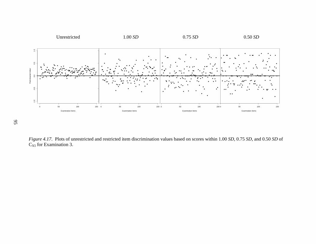
Unrestricted 1.00 SD 0.75 SD 0.50 SD
Figure 4.17. Plots of unrestricted and restricted item discrimination values based on scores within 1.00 SD, 0.75 SD, and 0.50 SD of CX5 for Examination 3.
0 50 100 150
-1.0
-0.5
0.0
0.5
1.0
Examination Items
Poi
nt-b
iser
ial V
alue
0 50 100 150
Examination Items
0 50 100 150
Examination Items
0 50 100 150
Examination Items
95

96
Figure 4.18. Boxplot highlighting distribution of item discrimination values under each condition for Examination 3.
unre
stric
ted
cx1_
1sd
cx1_
.75s
d
cx1_
.50s
d
cx2_
1sd
cx2_
.75s
d
cx2_
.50s
d
cx3_
1sd
cx3_
.75s
d
cx3_
.50s
d
cx4_
1sd
cx4_
.75s
d
cx4_
.50s
d
cx5_
1sd
cx5_
.75s
d
cx5_
.50s
d
-0.75
-0.50
-0.25
0.00
0.25
0.50
0.75
Poi
nt-b
iser
ial V
alue

97
Table 4.10
Descriptive Statistics of Discrimination Values Calculated for Examination 3
Cut Score Group M SD Min Max Range Skew n Unrestricted
0.16
0.13
-0.11
0.46
0.58
-0.02
76
CX1 +/- 1.00 SD
0.08 0.17 -0.29 0.57 0.86 0.34 37
+/- 0.75 SD
0.06 0.19 -0.42 0.52 0.94 0.09 25
+/- 0.50 SD
0.04 0.23 -0.44 0.70 1.14 0.30 17
CX2 +/- 1.00 SD
0.08 0.15 -0.36 0.49 0.84 0.18 43
+/- 0.75 SD
0.06 0.17 -0.42 0.49 0.90 0.04 36
+/- 0.50 SD
0.05 0.21 -0.52 0.54 1.06 -0.12 25
CX3 +/- 1.00 SD
0.08 0.19 -0.37 0.69 1.06 0.36 23
+/- 0.75 SD
0.06 0.20 -0.39 0.55 0.94 0.37 20
+/- 0.50 SD
0.04 0.29 -0.62 0.86 1.47 0.24 11
CX4 +/- 1.00 SD
0.09 0.13 -0.21 0.37 0.58 -0.10 52
+/- 0.75 SD
0.06 0.16 -0.35 0.50 0.85 -0.02 33
+/- 0.50 SD
0.05 0.19 -0.41 0.55 0.96 -0.08 26
CX5 +/- 1.00 SD
0.06 0.28 -0.62 0.86 1.48 0.25 13
+/- 0.75 SD
0.05 0.34 -0.77 0.83 1.60 0.16 8
+/- 0.50 SD 0.04 0.42 -0.88 0.88 1.76 0.29 6

98
The correlation matrix for Examination 3 is included in Table 4.11. Unlike the
previous examinations considered, far fewer correlations were significant for Examination 3.
Among the 120 correlation coefficients calculated, only 78 were found to be significantly
different than zero at the α = 0.05 level of significance. In addition, 42 coefficients expressed
negative relationships, which was more than both Examination 1 (12) and Examination 2
(24). The strongest correlation existed between the set of values calculated using scores
within 1.00 SD of CX2 and the set that included scores within 0.75 SD of CX2, r(147) = 0.79,
p < .001.
One-way repeated measures ANOVA was also conducted with respect to
Examination 3. Unlike the previous examinations, however, the Shapiro-Wilk normality test
(R Core Team, 2012) identified several groups of data for which the null hypothesis of
normality was rejected. The problematic groups were those calculated using scores within
0.75 SD of CX3, 0.50 SD of CX3, 0.75 SD of CX5, and 0.50 SD of CX5. An analysis of group
skewness values, however, indicated that each fell within -1.00 to 1.00. These values are
included in Table 4.10. Once again, therefore, the decision was made to proceed with the
ANOVA.
The assumption of sphericity was also violated, with Mauchly’s (1940) test producing
a significant result, W < 0.001, p < .001. The Greenhouse-Geisser (1959) correction, ε =
0.28, was applied to the degrees of freedom to correct the positively biased F-statistic. As
seen in Table 4.12, the results of the ANOVA were significant, F(4.20, 621.60) = 2.989, p =
.016. The results indicated the presence of a significant difference between at least two of
the group means.

Table 4.11
Correlation Matrix of Item Discrimination Values Calculated for Examination 3
CX1 CX2 CX3 CX4 CX5 UNR 1.00 SD 0.75 SD 0.50 SD 1.00 SD 0.75 SD 0.50 SD 1.00 SD 0.75 SD 0.50 SD 1.00 SD 0.75 SD 0.50 SD 1.00 SD 0.75 SD 0.50 SD
UNR 1.00 CX1
1.00 SD 0.47* 1.00 0.75 SD 0.13 0.52* 1.00 0.50 SD -0.06 0.10 0.44* 1.00 CX2
1.00 SD 0.46* 0.55* 0.27* 0.22* 1.00 0.75 SD 0.28* 0.50* 0.14 -0.04 0.79* 1.00 0.50 SD 0.25* 0.56* 0.15 -0.30* 0.51* 0.66* 1.00 CX3
1.00 SD 0.38* 0.13 0.09 0.26* -0.08 -0.28* -0.31* 1.00 0.75 SD 0.33* 0.36* 0.21* 0.14 -0.05 -0.23* -0.26* 0.69* 1.00 0.50 SD 0.26* 0.32* -0.08 -0.43* -0.23* -0.31* -0.08 0.32* 0.56* 1.00 CX4
1.00 SD 0.67* 0.20* -0.12 -0.39* 0.38* 0.28* 0.44* -0.17* -0.14 0.15 1.00 0.75 SD 0.36* -0.16 -0.28* -0.21* 0.20* -0.01 -0.24* 0.05 0.17* 0.14 0.43* 1.00 0.50 SD 0.20* -0.22* -0.44* -0.10 0.34* 0.08 -0.23* 0.12 0.04 0.10 0.29* 0.64* 1.00 CX5
1.00 SD 0.38* -0.01 -0.29* -0.37* -0.18* -0.25* -0.10 0.72* 0.46* 0.58* 0.11 0.19* 0.19* 1.00 0.75 SD 0.28* -0.18* -0.39* -0.37* -0.04 0.11 0.07 0.49* 0.04 0.03 0.14 0.11 0.19* 0.69* 1.00 0.50 SD 0.21* -0.25* -0.34* 0.09 0.11 0.07 -0.02 0.45* -0.10 -0.30* 0.02 0.06 0.11 0.50* 0. 75* 1.00 Note. * p = < .05.
99

100
Table 4.12
Results of the One-way Repeated Measures ANOVA for Examination 3
Source Model SS df MS F p Condition Sphericity Assumed 2.104 15.000 0.140 2.989 < .001* Greenhouse-Geisser
Corrected 2.104 4.200 0.501 2.989 .016*
Error Sphericity Assumed 104.188 2220.00 0.047 Greenhouse-Geisser
Corrected 104.188 621.600 0.168
Note. The Greenhouse-Geisser correction, estimated at ε = 0.28, was used to correct for the violation of the sphericity assumption. * = Significant at α = .05 level of significance.
The results of Tukey’s HSD test are included in Table 4.13. Unlike Examinations 1
and 2, significant differences were not observed between the unrestricted set of values and
each of the restricted groups. Significant differences were not observed between the
unrestricted group and four of the restricted groups. The groups between which a significant
difference with the unrestricted set was not observed included values calculated using scores
with 1.00 SD of CX1, 1.00 SD of CX2, 1.00 SD of CX3, and 1.00 SD of CX4. Significant
differences between the unrestricted group and each of the other sets, however, were
identified, with the mean unrestricted discrimination value being greater than the mean
values of the restricted groups.
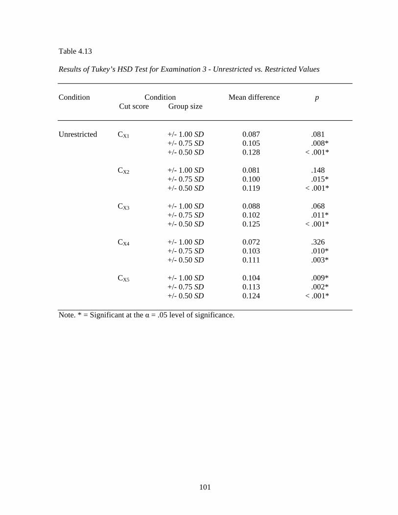
101
Table 4.13 Results of Tukey’s HSD Test for Examination 3 - Unrestricted vs. Restricted Values Condition Condition Mean difference p Cut score Group size Unrestricted CX1 +/- 1.00 SD 0.087 .081 +/- 0.75 SD 0.105 .008* +/- 0.50 SD 0.128 < .001* CX2 +/- 1.00 SD 0.081 .148 +/- 0.75 SD 0.100 .015* +/- 0.50 SD 0.119 < .001* CX3 +/- 1.00 SD 0.088 .068 +/- 0.75 SD 0.102 .011* +/- 0.50 SD 0.125 < .001* CX4 +/- 1.00 SD 0.072 .326 +/- 0.75 SD 0.103 .010* +/- 0.50 SD 0.111 .003* CX5 +/- 1.00 SD 0.104 .009* +/- 0.75 SD 0.113 .002* +/- 0.50 SD 0.124 < .001* Note. * = Significant at the α = .05 level of significance.

102
Summary – Research Question 1
For Research Question 1, results of the analysis based on visual comparisons
suggested that at each cut score location, the unrestricted set of discrimination values was, on
average, greater in value than the restricted sets. This was evident in both the plots and
boxplots. It was particularly true for Examinations 1 and 2, but less apparent for
Examination 3, which, according to sample size, was the smallest examination used in the
study. The results of the ANOVA supported this initial assessment, indicating that for
Examinations 1 and 2, the difference between the unrestricted set of discrimination values
and the sets of restricted values was statistically significant. In the case of Examination 3,
the difference between the unrestricted set of discrimination values and 11 of the 15
restricted sets was significant. Where significant differences were found, the mean
unrestricted point-biserial was larger than the mean restricted item discrimination value.

103
Research Question 2
Research Question 2 examined the degree to which using restricted item
discrimination values affected item selection, examination reliability, and classification
decision consistency. The results of the procedures conducted to answer this research
question for each examination are included in the sections that follow.
Examination 1
To examine the effect restricted item discrimination values had on item selection, two
50-item forms were created. Form A included the 50 most discriminating items from
Examination 1, using unrestricted point-biserials as the criterion for selection. Form B
included the 50 most discriminating items, using restricted point-biserials as the selection
criterion. The set of restricted values used to create Form B was based on scores within 1.00
SD of CX1. Descriptive statistics for the Examination 1 forms, as well as for those associated
with the other examinations used in the study, are included in Table 4.14.
The items selected for Form A and Form B are included in Table 4.15. As indicated
in the table, selecting items based on their restricted point-biserial value, as opposed to their
unrestricted value, resulted in Form B including 19 items that were not included in Form A.
The test variants for Examination 1, as well as for Examinations 2 and 3, therefore,
included both similar and dissimilar items. Because each form included items that were also
included on its corresponding test variant, dependent samples tests were used when
evaluating differences in reliability and decision consistency. For each test conducted,
however, a similar test using independent sample procedures was also performed. In each
case, the result of the independent samples test was identical to the dependent samples test.

104
Descriptive statistics were calculated for the discrimination values associated with
both forms. As seen in Table 4.16, the mean discrimination value for Form A, M = 0.39 (SD
= 0.08) was slightly larger than the mean value for Form B, M = .37 (SD = 0.09). To further
investigate the difference in mean discrimination values, however, a dependent samples t-test
was conducted.

Table 4.14
Descriptive Statistics of Test Forms A and B – All Examinations
Exam Form M SD Min Max Range Skew n α SEM κ* κ 95% CI 1
Form A
32.47 8.94 5.00 49.00 44.00 -0.49 490 0.89 3.01 0.69(.01) [0.67, 0.71]
Form B
30.94 8.65 6.00 48.00 42.00 -0.23 490 0.87 3.13 0.67(.01) [0.65, 0.69]
2 Form A
33.34 8.16 8.00 49.00 41.00 -0.49 161 0.87 2.94 0.66(.02) [0.62, 0.70]
Form B
34.32 7.59 17.00 49.00 32.00 -0.32 161 0.85 2.94 0.63(.02) [0.59, 0.68]
3 Form A
38.97 6.22 24.00 49.00 25.00 -0.62 76 0.83 2.59 0.59(.04) [0.51, 0.67]
Form B
39.76 5.45 25.00 47.00 22.00 -0.94 76 0.78 2.55 0.52(.05) [0.43, 0.62]
Note. * Numbers in parentheses indicate SE for κ.
104
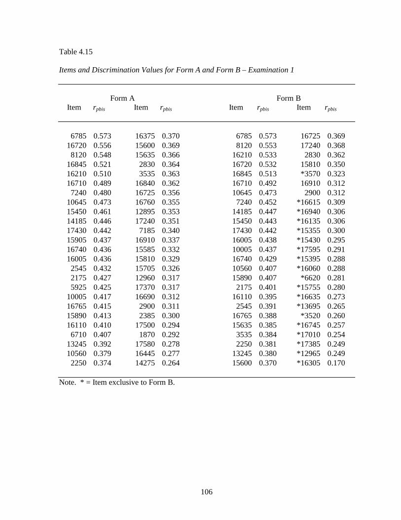
106
Table 4.15 Items and Discrimination Values for Form A and Form B – Examination 1 Form A Form B Item rpbis Item rpbis Item rpbis Item rpbis
6785 0.573 16375 0.370 6785 0.573 16725 0.369 16720 0.556 15600 0.369 8120 0.553 17240 0.368 8120 0.548 15635 0.366 16210 0.533 2830 0.362
16845 0.521 2830 0.364 16720 0.532 15810 0.350 16210 0.510 3535 0.363 16845 0.513 *3570 0.323 16710 0.489 16840 0.362 16710 0.492 16910 0.312 7240 0.480 16725 0.356 10645 0.473 2900 0.312
10645 0.473 16760 0.355 7240 0.452 *16615 0.309 15450 0.461 12895 0.353 14185 0.447 *16940 0.306 14185 0.446 17240 0.351 15450 0.443 *16135 0.306 17430 0.442 7185 0.340 17430 0.442 *15355 0.300 15905 0.437 16910 0.337 16005 0.438 *15430 0.295 16740 0.436 15585 0.332 10005 0.437 *17595 0.291 16005 0.436 15810 0.329 16740 0.429 *15395 0.288 2545 0.432 15705 0.326 10560 0.407 *16060 0.288 2175 0.427 12960 0.317 15890 0.407 *6620 0.281 5925 0.425 17370 0.317 2175 0.401 *15755 0.280
10005 0.417 16690 0.312 16110 0.395 *16635 0.273 16765 0.415 2900 0.311 2545 0.391 *13695 0.265 15890 0.413 2385 0.300 16765 0.388 *3520 0.260 16110 0.410 17500 0.294 15635 0.385 *16745 0.257 6710 0.407 1870 0.292 3535 0.384 *17010 0.254
13245 0.392 17580 0.278 2250 0.381 *17385 0.249 10560 0.379 16445 0.277 13245 0.380 *12965 0.249 2250 0.374 14275 0.264 15600 0.370 *16305 0.170
Note. * = Item exclusive to Form B.
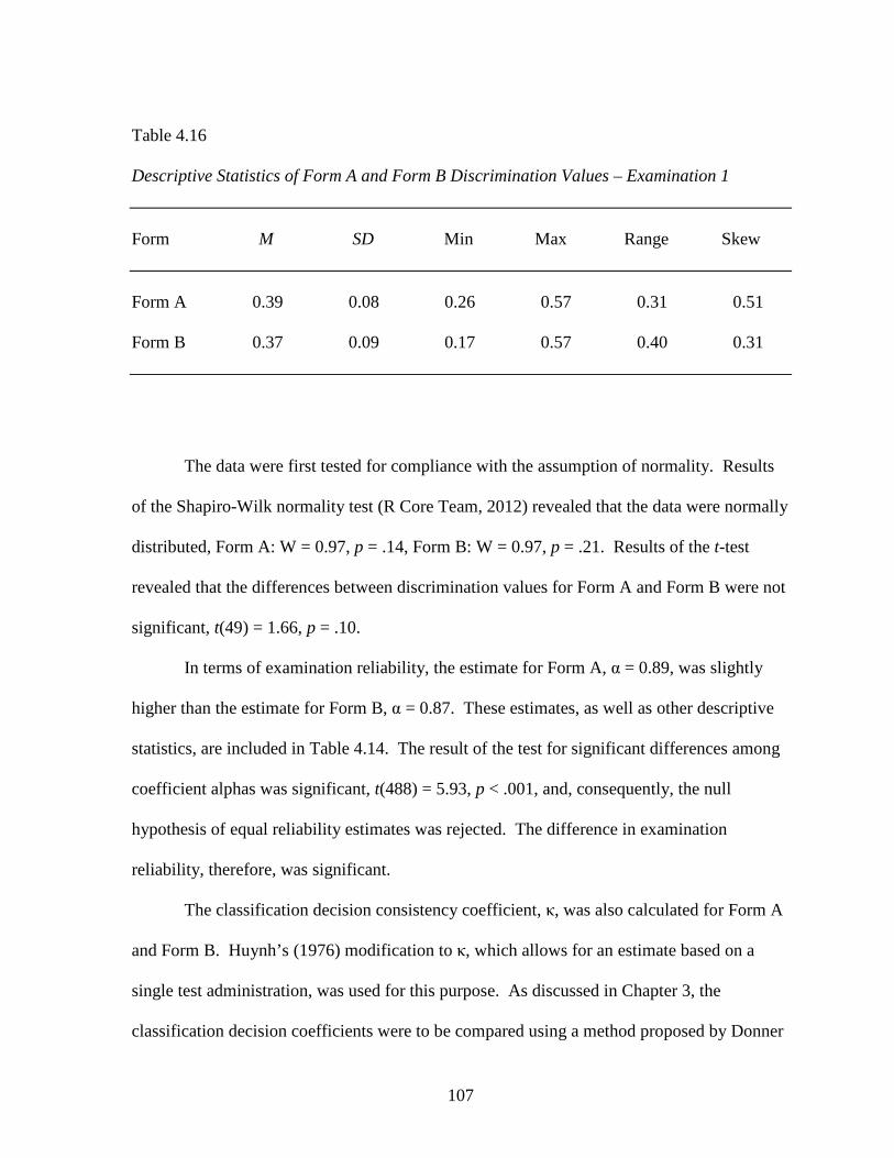
107
Table 4.16 Descriptive Statistics of Form A and Form B Discrimination Values – Examination 1 Form M SD Min Max Range Skew Form A 0.39 0.08 0.26 0.57 0.31 0.51 Form B 0.37 0.09 0.17 0.57 0.40 0.31
The data were first tested for compliance with the assumption of normality. Results
of the Shapiro-Wilk normality test (R Core Team, 2012) revealed that the data were normally
distributed, Form A: W = 0.97, p = .14, Form B: W = 0.97, p = .21. Results of the t-test
revealed that the differences between discrimination values for Form A and Form B were not
significant, t(49) = 1.66, p = .10.
In terms of examination reliability, the estimate for Form A, α = 0.89, was slightly
higher than the estimate for Form B, α = 0.87. These estimates, as well as other descriptive
statistics, are included in Table 4.14. The result of the test for significant differences among
coefficient alphas was significant, t(488) = 5.93, p < .001, and, consequently, the null
hypothesis of equal reliability estimates was rejected. The difference in examination
reliability, therefore, was significant.
The classification decision consistency coefficient, κ, was also calculated for Form A
and Form B. Huynh’s (1976) modification to κ, which allows for an estimate based on a
single test administration, was used for this purpose. As discussed in Chapter 3, the
classification decision coefficients were to be compared using a method proposed by Donner

108
et al. (2000). Upon further investigation, however, the method required the κ coefficients to
be based on multiple test administrations. This was not possible for the data used in this
study. Additional studies and models were considered, but each required the classification
decision consistency coefficients to be based on multiple test administrations (Barnhart &
Williamson, 2002; McKenzie et al., 1996; Williamson, Lipsitz, & Manatunga, 2000) or to
utilize independent samples (Fleiss, 1981; Lipsitz, Williamson, Klar, Ibrahim, & Parzen,
2001). Whereas no identified model for testing significant differences in κ coefficients fit the
data and context used in this study (κ based on dependent samples from a single test
administration), a test was not possible. The comparison of classification decision
consistency coefficients, therefore, was limited to an analysis of their associated 95%
confidence intervals. These intervals are included in Table 4.14.
A degree of caution should be used when characterizing differences between
statistics using confidence intervals. Whereas one may conclude that a significant difference
at the α = .05 level of significance exists when 95% confidence intervals do not overlap, it
may be misleading to suggest that a significant difference does not exist when the confidence
intervals do overlap. Previous research has shown that statistics with overlapping confidence
intervals may, in fact, be significantly different (Odeuyungbo, Thabane, & Markle-Reid,
2009). As seen in Table 4.14, the classification decision consistency estimate for Form A, κ
= 0.69 (SE = 0.01, 95% CI [0.67, 0.71]) was slightly higher than that of Form B, κ = 0.67 (SE
= 0.01, 95% CI [0.65, 0.69]. Had the 95% confidence intervals not overlapped, the null
hypothesis of no significant difference between κ coefficients could have been rejected. In
this case, however, the confidence intervals did overlap. It is plausible, although not a

109
certainty, therefore, that there is no significant difference between the classification decision
consistency coefficients associated with Form A and Form B.
Examination 2
The procedures used to create Form A and Form B for Examination 1 were also
conducted for Examination 2. As seen in Table 4.17, using restricted point-biserials resulted
in Form B including 22 items that were not included in Form A.
Descriptive statistics for the discrimination values associated with the Examination 2
forms are included in Table 4.18. Once again, the mean item discrimination value was
slightly larger for Form A, M = 0.37 (SD = 0.05), than it was for Form B, M = 0.35 (SD =
0.08). A dependent samples t-test was conducted to test for differences among the group
means. The Shapiro-Wilk normality test (R Core Team, 2012) indicated that the data
approximated normality, W = 0.98, p = .41. Results of the t-test indicated that the difference
between mean discrimination values was not significant, t(49) = 1.90, p = .06.

110
Table 4.17 Items and Discrimination Values for Form A and Form B – Examination 2 Form A Form B Item rpbis Item rpbis Item rpbis Item rpbis
108153 0.524 108155 0.363 108153 0.545 108162 0.338 108486 0.454 108507 0.363 108143 0.502 *60242 0.337 90390 0.450 108146 0.361 108486 0.487 108494 0.336
108492 0.448 59231 0.360 40885 0.443 *40944 0.333 108178 0.443 94586 0.358 90390 0.437 *51781 0.331 108143 0.436 108162 0.357 108487 0.435 *108478 0.328 108138 0.428 108189 0.356 108178 0.434 *108479 0.326 40885 0.423 108494 0.354 51787 0.432 *108144 0.323 51787 0.417 51793 0.348 62140 0.423 *41645 0.321 62140 0.413 108487 0.346 108154 0.423 *108198 0.320 40655 0.413 108182 0.346 40969 0.418 *62132 0.319 94582 0.407 94566 0.338 40992 0.418 108189 0.318 40969 0.402 108156 0.338 41181 0.415 62136 0.316
108509 0.397 108515 0.330 108176 0.409 *108193 0.307 108489 0.394 108166 0.327 94582 0.395 *108197 0.297 108477 0.394 84442 0.326 40655 0.387 *90398 0.265 108154 0.390 108201 0.324 84442 0.376 108515 0.264 40992 0.389 59149 0.319 *108187 0.372 *108481 0.255
108177 0.389 108506 0.317 94566 0.369 *108512 0.252 41181 0.385 108180 0.303 108492 0.366 *108488 0.242 51817 0.380 40668 0.303 108138 0.364 *90400 0.240 40657 0.379 108152 0.298 *59128 0.350 *108158 0.228
108176 0.375 108483 0.295 60258 0.349 *62135 0.225 108204 0.373 60258 0.292 108180 0.343 *108502 0.170 62136 0.368 108167 0.284 108477 0.340 *59138 0.157
Note. * = Item exclusive to Form B.

111
Table 4.18 Descriptive Statistics of Form A and Form B Discrimination Values – Examination 2 Form M SD Min Max Range Skew Form A 0.37 0.05 0.28 0.52 0.24 0.47 Form B 0.35 0.08 0.16 0.55 0.39 -0.07
As indicated in Table 4.14, the examination reliability estimate for Form A, α = 0.87,
was slightly larger than the estimate for Form B, α = 0.85. Further analysis also revealed that
the difference between examination reliability estimates was significant, t(159) = 2.20, p =
.03. Thus, the null hypothesis of equal coefficient alphas was rejected.
In terms of classification decision consistency, the κ coefficient associated with Form
A, κ = 0.66 (SE = 0.02, 95% CI [0.62, 0.70]) was slightly greater than the estimate for Form
B, κ = 0.63 (SE = 0.02, 95% CI [0.59, 0.68]). As was the case with Examination 1, the
confidence intervals for the forms associated with Examination 2 overlapped. A similar
conclusion, therefore, may be made: It is plausible that the observed difference in
classification decision consistency between Form A and Form B is not statistically
significant.

112
Examination 3
For Examination 3, the use of restricted point-biserials resulted in Form B including
22 items that were not included in Form A. These items are annotated in Table 4.19.
Descriptive statistics for the discrimination values for Form A and Form B are included in
Table 4.20. The mean discrimination value for Form A, M = 0.33 (SD = 0.08), was slightly
higher than that of Form B, M = 0.29 (SD = 0.13). Prior to conducting the t-test, the values
were also tested for normality. The Shapiro-Wilk test (R Core Team, 2012) revealed that the
data were normally distributed, Form A: W = 0.98, p = .74, Form B: W = 0.97, p = .18.
Results of the test indicated that the difference between mean discrimination values was not
significant, t(49) = 1.85, p = .07.
Examination reliability estimates were also calculated for the Examination 3 forms.
As indicated in Table 4.14, the reliability estimate for Form A, α = 0.83, was again larger
than the estimate for Form B, α =0.78. Once again, further analysis revealed that the
difference between examination reliability estimates was significant, t(74) = 2.10, p = .04.
Finally, Form A and Form B were compared with regard to classification decision
consistency. As seen in Table 4.14, the estimate for Form A, κ = 0.59 (SE = 0.04, 95% CI
[0.51, 0.67]) was larger than for Form B, κ = 0.52 (SE = 0.05, 95% CI [0.43, 0.62]).

113
Table 4.19 Items and Discrimination Values for Form A and Form B – Examination 3 Form A Form B Item rpbis Item rpbis Item rpbis Item rpbis
160005 0.540 160048 0.313 160084 0.518 160050 0.310 160041 0.467 160549 0.311 160552 0.516 *160021 0.309 160557 0.455 160055 0.311 160057 0.483 160048 0.307 160034 0.449 160056 0.309 160030 0.464 160064 0.265 160057 0.443 160548 0.308 160074 0.464 160053 0.261 160032 0.443 160011 0.306 160005 0.458 *160013 0.260 160051 0.419 160558 0.306 159998 0.444 160028 0.240 160541 0.417 160559 0.305 160032 0.443 *160047 0.228 160550 0.407 160573 0.298 160557 0.442 *160026 0.214 160029 0.402 160569 0.295 160041 0.422 *160020 0.208 160030 0.400 159999 0.293 160541 0.404 *160578 0.207 159998 0.399 160526 0.290 160051 0.402 *160536 0.200 160074 0.396 160535 0.285 160079 0.398 *160577 0.197 160555 0.396 160018 0.276 160550 0.396 *160025 0.190 160079 0.392 160050 0.263 160055 0.392 *159996 0.176 159997 0.378 160028 0.261 160014 0.365 *160527 0.167 160552 0.367 160035 0.253 160526 0.355 *160072 0.156 160006 0.366 160570 0.247 *160031 0.352 *160039 0.140 160084 0.353 160572 0.245 160006 0.346 *160554 0.129 160547 0.343 160064 0.242 *160540 0.332 *160533 0.125 160564 0.336 160059 0.233 160035 0.331 *160000 0.110 160014 0.335 160046 0.218 160034 0.330 *160575 0.077 160556 0.335 160566 0.196 160564 0.324 *160090 0.074 160537 0.333 160017 0.178 160535 0.312 *160545 0.057 160053 0.315 160089 0.175 159999 0.312 *160568 0.053
Note. * = Item exclusive to Form B.

114
Table 4.20 Descriptive Statistics of Form A and Form B Discrimination Values – Examination 3 Form M SD Min Max Range Skew Form A 0.33 0.08 0.18 0.54 0.37 0.19 Form B 0.29 0.13 0.05 0.52 0.46 -0.14
Once again, the 95% confidence intervals overlapped, suggesting that a conclusion similar to
those drawn regarding the other examinations may be made: It is plausible that the
differences in κ between Form A and Form B are not statistically significant.
Summary – Research Question 2
The procedures conducted to answer Research Question 2 suggested that using
restricted point-biserials as the criterion for selection significantly affected the items selected.
For Examination 1, 19 of the 50 items selected for Form B were not selected for Form A.
For Examinations 2 and 3, 22 of the 50 items selected for Form B were not selected for Form
A. Analysis of the item discrimination values indicated that the difference in mean point-
biserial between forms for each examination was not significant. The results also revealed,
however, a significant difference in examination reliability. For each examination, the
observed reliability estimate for Form A was slightly larger than that of Form B. In each
case, further analysis found the difference in reliability between forms to be statistically
significant. Finally, classification decision consistency was calculated for each form.

115
Observed estimates revealed that the κ coefficient associated with Form A was larger than
that of Form B for each examination. Analysis of the 95% confidence intervals, however,
prevented a rejection of the null hypothesis of equal classification decision consistency
estimates. It is plausible, therefore, that the observed difference between forms was not
statistically significant. Further discussion and analysis of the results presented here are
included in Chapter 5.

116
CHAPTER 5
DISCUSSION
Three areas of test development were emphasized in this study. First, the role item
discrimination plays in the test development process was a key aspect of the research.
Second, competency examinations used to credential individuals served as the context.
Third, the study replicated the realistic conditions that many developers of credentialing
examinations face by using relatively small samples of examinees, which, consequently,
necessitated the use of classical test theory procedures. Previous research has been devoted
to each of these areas individually. Prior to this study, however, no published research has
examined the ways in which these areas interact. As such, the research represents a unique
contribution to the field of test development.
No study, however, is without limitations. This chapter begins with an outline of
limitations that affected the research. Next, a discussion of the study’s key findings,
specifically as they relate to the research questions, is provided. This is followed by
recommendations for future research, practical implications for developers of examinations
that incorporate cut scores to foster categorical decisions about examinees (e.g., credentialing
examinations), and conclusions.
Limitations
The study was affected by two general limitations. These limitations are presented
below and are discussed in greater detail in the sections that follow.

117
1. The items used in the analysis were included in the final versions of their respective
examinations. As such, they potentially may have been more vetted than the types of
items typically under consideration during the item analysis phase of test
development, which this study sought to replicate.
2. The criteria by which items were selected for the Form A and Form B test variants
potentially did not wholly correspond to methods used by those who develop
credentialing examinations.
Refinement of Items Used in the Study
In many ways, this study attempted to replicate certain aspects of the process by
which credentialing examinations are developed. Like other types of tests, the process used
to develop credentialing examinations includes well-established steps. These steps were
highlighted in Table 1.1, which was adapted from research conducted by Downing (2006).
As seen in the table, item analysis typically occurs during the eighth step in this process, a
step labeled “scoring test responses.” During this stage of development, analysis of field-
tested items frequently occurs. One component of this analysis is the calculation and
evaluation of item discrimination values.
The procedures conducted in this study, specifically as they relate to Research
Question 2, sought to imitate item analysis. Item discrimination values were calculated and
used, for example, to select items for the Form A and Form B test variants just as they might
be used by test developers to select items for a credentialing examination. The items
included in these forms were then used to answer Research Question 2. For the items used in

118
this study, however, the process of item analysis had already occurred. These items were
included in the final version of each of their respective examinations, and, therefore, were
presumably selected over other less qualified items. The process of item analysis also may
have resulted in some form of modification to the items, such as changes in wording or order
of response options. A more accurate replication of the item analysis phase of test
development might include items that had not yet been selected for inclusion in the final
version of an examination, but which, along with many other items, were under consideration
for inclusion in the final version.
Although this limitation represents a slight deviation from the typical conditions
under which credentialing examination are normally developed, it is unlikely that it affected
the study’s overall findings. The research conducted was focused on the degree to which
using restricted point-biserials affected the discrimination values themselves, item selection,
examination reliability, and classification decision consistency. In each instance, the results
of the research with respect to the dependent variables just named would likely not have been
different had items in earlier phases of development been used. Exploring the effect less
refined items might have, however, may be valuable and is discussed in greater detail in the
section outlining recommendations for future research.
Item Selection Criteria
Another limitation associated with the current research is that in creating the forms
used to answer Research Question 2, item discrimination served as the sole criterion for item
selection. Although discrimination is typically an important consideration when selecting

119
items for examinations, other factors, which were not considered here, may also determine
the degree to which an item is appropriate for inclusion.
One such consideration, for example, may be item difficulty, which, for items scored
dichotomously, represents the proportion of examinees who have answered the item correctly
(Crocker & Algina, 2008). Item difficulty may be of particular importance for examinations
for which examinees are classified into multiple categories, such as basic, proficient, and
advanced. For these types of examinations, developers may want to include several items
with difficulty levels that correspond to the various performance categories. Item
discrimination, in such instances, may be a secondary consideration.
In most cases, however, item statistics, to include both discrimination and difficulty,
are not the only factors that determine suitability for inclusion in final-version examinations.
According to Livingston (2006), “Statistics alone cannot determine which items on a test are
good and which are bad, but statistics can be used to identify items that are worth a
particularly close look” (p. 423). Other factors that influence the selection of items are based
on test specifications. Such specifications are sometimes referred to as test blueprints,
because they specify how the test or form is to be constructed (Schmeiser & Welch, 2006).
A test blueprint may specify, for example, that a certain number of items should be
associated with particular content standards. Using a third-grade mathematics examination
as an example, a test blueprint may direct that 20% of the items should be devoted to each of
the following: addition, subtraction, simple multiplication, geometry, and fractions. As
such, regardless of the statistics associated with items related to geometry, 20% of the items
must cover that content standard. Consequently, it is possible that a geometry-related item
with a relatively low item discrimination value may be selected, whereas an addition-related

120
item with a higher discrimination value may not. Test blueprints may also stipulate other
examination characteristics, such as the types of items to be used (i.e., constructed-response
versus selected–response formats), the ordering of items (i.e., based on difficulty or content
domain), test length, item scoring, and delivery specifications.
An important aspect of this study was the creation of the Form A and Form B test
variants used to answer Research Question 2. Because test blueprints were not available for
the examinations used in this research, item discrimination was the only criterion considered
when selecting items for inclusion in the pseudo-forms. Form A included the 50 most
discriminating items using unrestricted discrimination values as the selection criterion. Form
B included the 50 most discriminating items using restricted discrimination values as the
selection criterion. Had test blueprints been available, those specifications could have also
been considered. Examination 3, for example, measured nurses’ understanding of diabetes.
It is possible that the test blueprint required a certain number of items to cover risk factors for
diabetes, others to cover treatment of diabetes, and yet others to cover differences between
types of diabetes. Because test specifications were not available, considering these types of
issues in the item selection process was not possible.
It is important that the items selected for an examination match the requirements
outlined in the test specifications because the items represent portions of the content
standards. If the items do not sufficiently cover the content standards as specified by a test
blueprint, a case for the validity of the examination is more difficult to make. According to
Schmeiser and Welch (2006), “The domains to which test-score inferences are to be made
serve as examples of the sources of validity evidence that can be used” (p. 315).

121
Although the process used to select items for the Form A and Form B test variants did
not consider these additional factors, the results are still important with respect to the
relationship between restricted item discrimination values and those aspects of test
development examined in this study, namely, item selection, examination reliability, and
classification decision consistency. Item discrimination may not be the only factor
considered when selecting items for an examination, but it almost always is a factor of
consideration. Despite this limitation, therefore, the research findings presented here are still
important and relevant.
Key Findings
The results of the study produced four key findings: one related to Research Question
1 and three related to Research Question 2. The key findings are summarized below. Each
key finding is discussed in greater detail in the sections that follow.
1. Restricting the calculation of item discrimination values to scores of examinees at
or near anticipated cut scores resulted in lower discrimination values than those
calculated using all examinee scores. (Research Question 1)
2. Using restricted item discrimination values as the primary criterion for item
selection resulted in the selection of items that were different than those selected
using unrestricted item discrimination values. (Research Question 2)
3. Examinations comprised of items selected using restricted item discrimination
values as the primary selection criterion produced slightly lower reliability
estimates than examinations comprised of items selected using unrestricted item
122
discrimination values. Differences in reliability estimates between these
examinations were significantly greater than zero. (Research Question 2)
4. Examinations comprised of items selected using restricted item discrimination
values as the primary selection criterion produced slightly lower observed
classification decision consistency estimates than examinations comprised of
items selected using unrestricted item discrimination values. The degree to which
these differences were statistically significant, however, was uncertain. (Research
Question 2)
Effect on Item Discrimination Values
The purpose of Research Question 1 was to determine the effect limiting
discrimination values to scores of examinees near real or anticipated cut scores had on item
discrimination values. To answer this question, procedures were followed that resulted in the
creation of 15 sets of restricted item discrimination values. The sets of restricted values were
based on scores within 1.00 SD, 0.75 SD, and 0.50 SD of five distinct cut score locations. As
observed in Table 5.1, in all cases, mean restricted item discrimination values were smaller
than corresponding mean unrestricted item discrimination values. For Examinations 1 and 2,
the results of one-way ANOVA analysis indicated that the difference between the
unrestricted set of discrimination values and each of the 15 sets of restricted discrimination
values was significantly greater than zero. This was also the case for all but four of the sets
of restricted discrimination values in Examination 3.
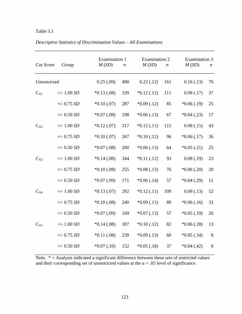
123
Table 5.1
Descriptive Statistics of Discrimination Values – All Examinations
Examination 1 Examination 2 Examination 3
Cut Score Group M (SD) n M (SD) n M (SD) n Unrestricted
0.25 (.09) 490 0.22 (.12) 161 0.16 (.13) 76
CX1 +/- 1.00 SD
*0.13 (.08) 339 *0.12 (.12) 111 0.08 (.17) 37
+/- 0.75 SD
*0.10 (.07) 287 *0.09 (.12) 85 *0.06 (.19) 25
+/- 0.50 SD
*0.07 (.08) 198 *0.06 (.13) 67 *0.04 (.23) 17
CX2 +/- 1.00 SD
*0.12 (.07) 317 *0.12 (.11) 115 0.08 (.15) 43
+/- 0.75 SD
*0.10 (.07) 267 *0.10 (.12) 96 *0.06 (.17) 36
+/- 0.50 SD
*0.07 (.08) 200 *0.06 (.13) 64 *0.05 (.21) 25
CX3 +/- 1.00 SD
*0.14 (.08) 344 *0.11 (.12) 93 0.08 (.19) 23
+/- 0.75 SD
*0.10 (.08) 255 *0.08 (.13) 76 *0.06 (.20) 20
+/- 0.50 SD
*0.07 (.09) 171 *0.06 (.14) 57 *0.04 (.29) 11
CX4 +/- 1.00 SD
*0.13 (.07) 292 *0.12 (.11) 109 0.09 (.13) 52
+/- 0.75 SD
*0.10 (.08) 240 *0.09 (.11) 89 *0.06 (.16) 33
+/- 0.50 SD
*0.07 (.09) 169 *0.07 (.13) 57 *0.05 (.19) 26
CX5 +/- 1.00 SD
*0.14 (.08) 307 *0.10 (.12) 82 *0.06 (.28) 13
+/- 0.75 SD
*0.11 (.08) 239 *0.09 (.13) 60 *0.05 (.34) 8
+/- 0.50 SD *0.07 (.10) 152 *0.05 (.18) 37 *0.04 (.42) 6 Note. * = Analysis indicated a significant difference between these sets of restricted values and their corresponding set of unrestricted values at the α = .05 level of significance.

124
One of the reasons the study incorporated three examinations, five distinct cut score
locations, and three different bands of examinee scores around those cut score locations was
to evaluate how each of those variables affected the results. For Examination 1, which was
the largest sample used in study (n = 490), and Examination 2, which was the second largest
sample used (n = 161), the location of the cut score appeared to have little influence on the
outcome of the results. Regardless of either the location of the cut score or the size of the
group around that cut score location considered, the difference between the resulting sets of
restricted discrimination values and the unrestricted set of discrimination values was found to
be significantly greater than zero. In all cases, the mean restricted discrimination values were
smaller than the mean unrestricted discrimination value.
Examination 3, which was the smallest sample used in the study (n = 76), produced
results similar to those identified for Examinations 1 and 2, with four exceptions. Although
the observed mean discrimination value for each of the sets of restricted values was smaller
than the unrestricted set, the difference between the unrestricted set and four of the restricted
sets was found to be not significantly greater than zero. Those four sets included values
based on scores within 1.00 SD of CX1, CX2, CX3, and CX4.
After completing the initial set of procedures used to answer Research Question 1, it
was determined that additional two-way ANOVA would be useful in determining the effect
cut score location and examinee score group size, as well as any possible interaction between
these two factors, had on restricted item discrimination values. The analysis was developed
using five levels for the cut score location factor (CX1, CX2, CX3, CX4, and CX5) and three
levels for the examinee score group size factor (1.00 SD, 0.75 SD, and 0.50 SD). The
procedure, like the one-way ANOVA conducted earlier, incorporated repeated measures.

125
Violations of the sphericity assumption, which affected each of the examinations, were
resolved using the Greenhouse-Geisser (1959) correction.
For each of the examinations used, there was no significant main effect for the cut
score location factor or for the interaction of cut score location and examinee score group
size. There was, however, a significant main effect for the factor representing the size of the
group of scores considered for each examination, Examination 1: F(1.20, 208.80) = 492.35, p
< .001; Examination 2: F(1.22, 243.97) = 161.84, p < .001; Examination 3: F(1.75, 259.59) =
14.62, p < .001. The analysis confirmed that cut score location did not significantly affect
the magnitude of the restricted item discrimination values. The examinee score group size
considered when calculating the discrimination values, however, did significantly affect the
restricted point-biserials. For each examination, as the size of the group of scores considered
decreased in size, so too did its associated mean item discrimination value.
After the procedures described in Chapter 3 were conducted, an evaluation of the
differences between unrestricted discrimination values and restricted values was conducted at
the item level. That is, for each item in each examination, differences between the
unrestricted discrimination value and the 15 sets of restricted values were examined. The
results of this analysis are included in Table 5.2. The table indicates the number of item
discrimination values for each examination that either increased or decreased when the
restricted conditions were considered.

126
Table 5.2
Change in Direction of Discrimination Values – All Examinations
Examination 1 Examination 2 Examination 3
Cut Score Group - ∆ (%) + ∆ (%) - ∆ (%) + ∆ (%) - ∆ (%) + ∆ (%) CX1 +/- 1.00 SD
169
(96.6%) 6
(3.4%) 165
(82.5%) 35
(17.5%) 106
(71.1%) 43
(28.9%) +/- 0.75 SD
172
(98.3%) 3
(1.7%) 167
(83.5%) 33
(16.5%) 106
(71.1%) 43
(28.9%) +/- 0.50 SD
168
(96.0%) 7
(4.0%) 168
(84.0%) 32
(16.0%) 102
(68.5%) 47
(31.5%) CX2 +/- 1.00 SD
170
(97.1%) 5
(2.9%) 175
(87.5%) 25
(12.5%) 109
(73.2%) 40
(26.8%) +/- 0.75 SD
174
(99.4%) 1
(0.6%) 175
(87.5%) 25
(12.5) 109
(73.2%) 40
(26.8%) +/- 0.50 SD
169
(96.6%) 6
(3.4%) 172
(86.0%) 28
(14.0%) 102
(68.5%) 47
(31.5%) CX3 +/- 1.00 SD
170
(97.1%) 5
(2.9%) 160
(80.0%) 40
(20.0%) 110
(73.8%) 39
(26.2%) +/- 0.75 SD
171
(97.7%) 4
(2.3%) 160
(80.0%) 40
(20.0%) 108
(72.5%) 41
(27.5%) +/- 0.50 SD
172
(98.3%) 3
(1.7%) 166
(83.0%) 34
(17.0%) 101
(67.8%) 48
(32.3%) CX4 +/- 1.00 SD
162
(92.6%) 13
(7.4%) 164
(82.0%) 36
(18.0%) 107
(71.8%) 42
(28.2%) +/- 0.75 SD
169
(96.6%) 6
(3.4%) 172
(86.0%) 28
(14.0%) 110
(73.8%) 39
(26.2%) +/- 0.50 SD
169
(96.6%) 6
(3.4%) 167
(83.5%) 33
(16.5%) 112
(75.2%) 37
(24.8%) CX5 +/- 1.00 SD
171
(97.7%) 4
(2.3%) 163
(81.5%) 37
(18.5%) 106
(71.1%) 43
(28.9%) +/- 0.75 SD
167
(95.4%) 8
(4.6%) 160
(80.0%) 40
(20.0%) 102
(68.5%) 47
(31.5%) +/- 0.50 SD 166
(94.9%) 9
(5.1%) 160
(80.0%) 40
(20.0%) 93
(62.4%) 56
(37.6%)

127
As seen in the table, the discrimination value associated with the vast majority of
examination items decreased when a subset of examinee scores was used to calculate the
point-biserials. This was particularly true for Examination 1, where the discrimination values
of 174 of the 175 items, or 99.4%, decreased in size when their calculation was limited to
examinee scores within 0.75 SD of CX2. This was the largest percentage of change in either
direction for any group of restricted values across all examinations. For Examination 2, as
many as 87.5% of unrestricted point-biserials decreased in value when restricted conditions
were applied. The largest group of change in Examination 3 was associated with values
calculated using scores within 0.50 SD of CX4. For this group, 75.2% of values decreased.
The relationship between the percentages of item discrimination values that decreased
under restricted conditions and the examination sample size may also be observed. The most
dramatic changes appear in the restricted sets associated with Examination 1, which included
the largest sample size. Those changes were less dramatic in Examinations 2 and 3, for
which the sample sizes were much smaller.
The observed decrease in discrimination values under restricted conditions was likely
due in part to the fact that the samples upon which restricted values were calculated were
more homogeneous than the samples upon which unrestricted values were calculated. As
observed earlier, a key component in the calculation of the point-biserial statistic is the
standard deviation of scores considered, which serves as the denominator in the formula:
(5.1)
ρpbis=µ +−µx
σ x
p / q
128
where µ+ is the mean total score for those who respond to the item correctly;
µx is the mean total score for the entire group of examinees;
σx is the standard deviation for the entire group of examinees;
p is item difficulty; and
q is equal to (1 - p) (Crocker & Algina, 2008).
All else being equal, therefore, smaller standard deviations for the group of scores
used in its calculation will result in smaller point-biserial statistics. In some cases, the
smaller, more homogeneous groups of scores, along with their smaller standard deviations,
resulted in positive point-biserials becoming negative. The standard deviations of the groups
of scores used to calculate the unrestricted discrimination values and the restricted values
based on scores within 1.00 SD of CX1 for each examination are included in Table 5.3. As
seen in the table, the standard deviation of scores used to calculate restricted discrimination
values are smaller than their corresponding unrestricted values. Although not included in
Table 5.3, the standard deviations for each group of restricted values becomes smaller in size
as the group used to calculate the values decreases in size. The standard deviations of groups
of scores within 1.00 SD of each cut score were closer to the standard deviation of all scores,
upon which the unrestricted values were calculated than were any of the other sets of
restricted values. This may explain why the only four sets of restricted values that were not
found to be significantly different than their corresponding unrestricted discrimination
values, as seen in Table 5.1, were each based on scores within 1.00 SD of their associated cut
score. The standard deviations of these groups of scores were closer to the standard
deviation of the unrestricted set than were any other sets of restricted values in Examination
3.

129
Table 5.3
Descriptive Statistics of Selected Groups of Scores
Exam Cut score Group n M SD Min Max Range 1 Unrestricted 490 111.42 19.55 46 161 115 CX1 +/- 1.00 SD 339 115.23 10.06 96 134 38 2 Unrestricted 161 134.27 18.30 82 174 92 CX1 +/- 1.00 SD 111 131.43 9.92 112 148 36 3 Unrestricted 76 115.04 9.01 93 134 41 CX1 +/- 1.00 SD 37 108.57 4.69 98 115 17
Effect on Item Selection
Using restricted item discrimination values as the criterion by which items were
selected resulted in the Form B test variant of each examination including numerous items
that were not included in the Form A variant, which utilized unrestricted values as the
selection criterion. The Form B variant of Examination 1, for instance, included 19 items
that were not included in the Form A variant. The Form B variant of Examinations 2 and 3
each contained 22 items that were not included in the Form A variants. These values, as well
as other descriptive statistics for the test variants used to answer Research Question 2, are
included in Table 5.4. They are also represented in Figure 5.1.

Table 5.4
Descriptive Statistics of Forms A and B Test Variants – All Examinations
No. Items Exam Form M SD Min Max Range Unique to n α SEM κ* κ 95% CI Form B 1
Form A
32.47 8.94 5.00 49.00 44.00 -- 490 0.89 3.01 0.69(.01) [0.67, 0.71]
Form B
30.94 8.65 6.00 48.00 42.00 19 490 0.87 3.13 0.67(.01) [0.65, 0.69]
2 Form A
33.34 8.16 8.00 49.00 41.00 -- 161 0.87 2.94 0.66(.02) [0.62, 0.70]
Form B
34.32 7.59 17.00 49.00 32.00 22 161 0.85 2.94 0.63(.02) [0.59, 0.68]
3 Form A
38.97 6.22 24.00 49.00 25.00 -- 76 0.83 2.59 0.59(.04) [0.51, 0.67]
Form B
39.76 5.45 25.00 47.00 22.00 22 76 0.78 2.55 0.52(.05) [0.43, 0.62]
Note. * Numbers in parentheses indicate SE for κ.
128

131
Examination 1 Examination 2 Examination 3
= Unique to Form B = Common to both forms
Figure 5.1. Pie charts representing breakdown of Form B test variant items for each examination.
This finding (i.e., that using restricted item discrimination values when evaluating
items for inclusion in the test variants resulted in the selection of items that were different
than selected using unrestricted discrimination values) is important because, in many ways, it
speaks to the validity of such examinations. The items unique to the Form B variants were
more discriminating for those examinees with total scores closest to the cut score, than were
the items unique to Form A. Again, according to the Standards (AERA et al., 1999), test
validity is “the degree to which evidence and theory support the interpretation of test scores
entailed by proposed uses” (p. 9). The interpretation of scores associated with credentialing
examinations is, of course, that those who pass are qualified to receive certification or
licensure. Selecting items that better discriminate among examinees with scores close to the
test cut score helps to support this interpretation.

132
This position is also supported by the previously mentioned work of Harris and
Subkoviak (1986), who proposed item selection criteria for mastery tests, of which
credentialing examinations are a form. Their words seem particularly relevant within the
context of the current discussion:
For a mastery test, this means selecting items that discriminate between masters and non-masters, as opposed to within masters and within non-masters. The consensus appears to be that a good mastery item is one which masters answer correctly and non-masters answer incorrectly. (p. 496)
Likewise, The Standards (AERA et al., 1999) make similar recommendations regarding the
importance of emphasizing examinees with total scores near cut scores:
Tests for credentialing need to be precise in the vicinity of the passing, or cut, score. They may not need to be precise for those who clearly pass or clearly fail. Sometimes a test used in credentialing is designed to be precise only in the vicinity of the cut score. (p. 157).
Although the use of restricted discrimination values may result in the selection of items that
are less discriminating for examinees who clearly pass or fail the examination, their use in
the item analysis phase of test development, as documented in this research, resulted in the
selection of items that better discriminate among examinees with scores in the vicinity of the
cut score. As such, their use supports the suggestions and recommendations outlined in the
preceding quotations.
It is also important to understand how the inclusion of items based on restricted
discrimination values affects the consistency with which candidates pass or fail the
examination. To gain a better understanding of this effect, a series of tables highlighting the
degree to which item selection affected pass/fail consistency were created. Figures 5.2, 5.3,
and 5.4 display pass/fail consistency comparisons between the full test and both test variants
for each of the examinations used in the study. In each of the figures, the cut score used for

133
the full examination was the actual cut score (CX1) and a proportionally comparable cut score
for the test variants.
Examination 1 (Full) Pass Fail
Form A (Examination 1)
Pass
Fail
212 47
22 209
Examination 1 (Full) Pass Fail
Form B (Examination 1)
Pass
Fail
203 29
31 227
Form A (Examination 1) Pass Fail
Form B (Examination 1)
Pass
Fail
223 9
36 222
Figure 5.2. Pass/fail consistency tables for Examination 1 and associated test variants.

134
Examination 2 (Full) Pass Fail
Form A (Examination 2)
Pass
Fail
91 7
11 52
Examination 2 (Full) Pass Fail
Form B (Examination 2)
Pass
Fail
97 5
5 54
Form A (Examination 2) Pass Fail
Form B (Examination 2)
Pass
Fail
90 15
8 48
Figure 5.3. Pass/fail consistency tables for Examination 2 and associated test variants.

135
Examination 3 (Full) Pass Fail
Form A (Examination 3)
Pass
Fail
54 0
10 12
Examination 3 (Full) Pass Fail
Form B (Examination 3)
Pass
Fail
59 2
5 10
Form A (Examination 3) Pass Fail
Form B (Examination 3)
Pass
Fail
54 7
0 15
Figure 5.4. Pass/fail consistency tables for Examination 3 and associated test variants. The effect item selection method and, consequently, examination composition had on
pass/fail rates may be observed in the figures. As seen in Figure 5.2, among those who
passed the full version of Examination 1, 22 examinees would have failed the Form A variant
and 31 would have failed the Form B variant.

136
The figure also illustrates the difference in pass/fail rates between the two test
variants. Among those who passed the Examination 1 Form A variant, 36 examinees would
have failed the Form B variant, which used restricted discrimination values to select items.
Among the candidates who passed the Form B variant, nine would have failed the Form A
variant, which used unrestricted discrimination values as the selection criterion. As
displayed in Figures 5.3 and 5.4, this was not the case for Examinations 2 and 3. For each of
those examinations, there were more examinees who passed the Form B variant (based on
restricted discrimination values) but failed the Form A variant (based on unrestricted
discrimination values) than examinees who passed the Form A but failed the Form B.
The method by which items were selected for inclusion in the test variants, therefore,
played an important and consequential role in determining who passed and who failed the
tests. For two of the examinations used in this study, the number of examinees who failed
the variant using unrestricted discrimination values but passed the variant using restricted
values was greater than those who passed the variant using unrestricted values but failed the
variant using restricted values.
Effect on Examination Reliability
For each of the examinations used in this study, scores associated with the Form B
test variant, which utilized restricted item discrimination values as the item selection
criterion, produced lower estimates of reliability than did the Form A variants, which used
unrestricted discrimination values to select items. The reliability estimates, expressed in
terms of coefficient alpha (Cronbach, 1951), are included in Table 5.4. Further analysis

137
found the differences in reliability estimates between the test variants for each examination to
be significantly greater than zero.
A primary consideration when explaining the lower reliability estimates associated
with the Form B variants may be their inclusion of unique items that were not included in the
Form A variants. As mentioned earlier in this chapter, the Examination 1 Form B variant
included 19 unique items. The Form B variant for Examinations 2 and 3 each included 22
unique items. The presence of these unique items led to lower total score variances for the
Form B test variants when compared to the Form A versions. As seen in Table 5.4, the
standard deviation of each Form B variant is lower than its corresponding Form A. Like the
point-biserial statistic, total test score variance is a factor in the calculations of coefficient
alpha:
α̂ −k
k−11−
Σσ̂ i2
σ̂ x2
(5.2)
where k is the number of items on the examination;
σ̂ i2 is the variance of item i; and
σ̂ x2 is the total test variance (Crocker & Algina, 2008).
Examinations with lower total test variance, consequently, generally produce lower estimates
of reliability.
A comparison of the unique items included in the Form B variants with the items that
would have been selected had unrestricted discrimination values been used to select items, as
was done with the Form A variants, is helpful in illustrating this point. These comparisons

138
are included in Table 5.5. As seen in the table, the items unique to Form B variants in each
case led to scores that produced lower standard deviations and lower estimates of reliability
when compared to the unique items included in their Form A counterparts. With the
exception of these items, the remaining items among the examination-specific test variants
were identical. The inclusion of the unique Form B items resulted in lower test score
variance, and, therefore, lower reliability estimates.
Table 5.5
Descriptive Statistics for Unique Form A and Form B Test Variant Items – All Examinations
Exam Form No. Items n M SD Min Max α SEM 1 Form A 19 490 13.69 3.09 1 19 0.68 1.74 Form B 19 490 12.16 2.93 3 18 0.57 1.93 2 Form A 22 161 14.06 3.75 2 21 0.73 1.96 Form B 22 161 15.05 3.11 7 21 0.60 1.96 3 Form A 22 76 16.79 2.94 5 22 0.66 1.72 Form B 22 76 17.58 2.02 13 21 0.31 1.67
The inclusion of items that better discriminate among examinees with total scores
nearest the examination cut score, therefore, appears to come at a cost. Whereas the use of
restricted discrimination values allowed items to be included that emphasized the region of

139
the cut score, it resulted in lower levels of test score variance and lower examination
reliability estimates.
A more important question in terms of this finding may be the degree to which
developers of credentialing examinations are willing to accept the lower estimate of
reliability that appear to be associated with the use of restricted discrimination values.
Reliability, not unlike validity, should be interpreted within the framework of the
examination’s purpose. According to Haertel (2006), “test score reliability must be
conceived relative to particular testing purposes and contexts” (p. 65). With the purpose of
credentialing examinations being placed squarely on the qualification of examinees to
receive certification or licensure, it may be possible that the validity-based benefits of using
restricted discrimination values outweigh the lower estimates of reliability.
Another important consideration regarding this balance may be the degree to which
the use of unrestricted discrimination values results in higher examination reliability
estimates. Although the differences in reliability estimates between the test variants were
found to be significantly greater than zero, the observed difference between variants was
relatively minor. The observed difference in the Examination 1 and 2 variants, for example,
was 0.02. The difference between Examination 3 variants was 0.05. Although there is no
official threshold for the acceptability of examination reliability estimates, it is seems
unlikely that such minor differences would be unacceptable to many test developers.
Effect on Classification Decision Consistency
The Form B test variants, for each examination used, produced lower observed
estimates of classification decision consistency, as expressed by coefficient κ, than did the

140
Form A variants. These observed values are included in Table 5.4. The lack of a test of
significant differences between coefficients κ based on dependent samples derived from a
single test administration precluded the possibility of hypothesis testing. Analysis of
differences, therefore, was limited to comparisons of 95% confidence intervals. Whereas
95% confidence intervals that do not overlap indicate differences that are significantly
greater than zero at the α = .05 level of significance, similar conclusions cannot be reached if
the confidence intervals do overlap. For each of the examinations used, the coefficient κ
95% confidence intervals overlapped. It is plausible, therefore, that the observed differences
are not significantly greater than zero. Statistically speaking, however, such a conclusion
cannot be made with certainty.
Within the context of using restricted item discrimination values as a criterion for
item selection, the interpretation of classification decision consistency coefficients is similar
to that of the examination reliability estimates. Although the observed coefficients
associated with the Form B test variants were lower than their Form A counterparts, the
differences were relatively minor. The observed difference between Examination 1 test
variants, for example, was 0.02. The differences between Examinations 2 and 3 variants
were 0.03 and 0.07 respectively. Coefficient κ is interpreted as the increase in decision
consistency over chance as a proportion of the maximum possible increase over chance
(Crocker & Algina, 2008). For the Form A variant associated with Examination 1, therefore,
69% of the total possible increase over chance consistency was observed. This figure was
67% for the Form B variant.
The primary question, therefore, may be the acceptability of slightly lower
classification decision consistency coefficients when restricted item discrimination values are

141
used. Again, the extent to which the differences between classification decision consistency
coefficients produced using unrestricted and restricted discrimination values are greater than
zero is not known. However, it seems unlikely that the relatively minor observed differences
would lead to the elimination of restricted values as a consideration when conducting item
analysis.
Recommendations for Future Research
While conducting the research, several recommendations for future research were
identified. These recommendations include:
1. Conduct research with items that have not previously gone through the process of
item analysis.
2. Conduct research using test specifications, or blueprints, to guide the selection of
items.
3. Develop longer test variants to assess the difference between tests with items selected
using restricted discrimination values and tests with items selected using unrestricted
values.
4. Examine the degree to which non-classical test theory approaches, such as item
response theory, support the findings of the current study.
5. Study how using restricted discrimination values affects the standard setting process.
Each recommendation is discussed in further detail in the sections that follow.
142
Conduct Research with Less Refined Items
The recommendation to conduct similar research with less refined items is based on a
limitation discussed earlier. Each of the three examinations used in this study included items
that had previously undergone the process of item analysis. As such, the items used had,
presumably, already met certain thresholds that validated their inclusion in the examination.
It is also possible that based on this analysis, the items maybe have been modified in certain
aspects, such as item or selected response wording.
Future research might examine the degree to which using less refined items, such as
those in actual banks of field-tested items, supports the results of the current study. Using
less refined items would more accurately replicate the process of item analysis, which, in
many ways, was the intent of the procedures conducted to answer Research Question 2.
Use Test Specifications to Guide Item Selection
Like the previous recommendation, this suggestion is tied to one of the study
limitations. In the process of creating the test variants used to answer Research Question 2,
item discrimination was the only criterion considered in selecting items. As mentioned
previously, in reality, it is much more likely that additional factors would be considered when
determining the suitability of items to be included in the final version of the examination.
Test specifications, or blueprints, stipulate the degree to which content standards
should be covered by examination items. The specifications are important because they tie
content standards to the knowledge, skills, and attributes measured by the examination. The
content standards are also important because, if developed correctly, they support the purpose
of the examination, and, consequently, serve as sources of test validity. Test specifications

143
were not available for the examinations used in the study. Future research might compare the
results of this study with procedures that incorporate test specifications. Had test blueprints
been available, the number of items unique to the Form B variants might have been different.
A comparison of this nature would provide more clarity to the findings of this study.
Develop Longer Tests to Assess Effects of Restricted Discrimination Values
Another recommendation for possible future research is to increase the scope of the
comparison between examinations developed using restricted item discrimination values and
those developed using unrestricted values. Whereas the procedures associated with the
current study included the creation of two 50-item examinations, the development of larger
examinations might provide more insight into the differences in examination reliability and
classification decision consistency estimates.
According to Crocker and Algina (2008), test length is one of several factors that
affect examination reliability estimates, with longer tests generally producing larger
reliability estimates. The differences in examination reliability between the 50-item test
variants considered in this study were found to be significantly greater than zero for each
examination. Further research, however, might explore the degree to which these findings
were consistent with much larger examinations. For example, test variants with between 100
and 200 items might produce reliability estimates that are much closer, and, potentially,
whose differences are not found to be significantly greater than zero. This may also be true
for classification decision consistency.

144
Use of Non-Classical Test Theory Approaches
The context under which this study was conducted purposefully attempted to replicate
the realistic conditions faced by many developers of credentialing examinations. That is, it
utilized examinations with relatively small sample sizes, which necessitated the use of
classical test theory. By doing so, the results of this study may be more generalizable to
those involved with the development of credentialing examinations.
Research aimed at other approaches used to calculate item discrimination values,
however, might help to expand the understanding of restricted discrimination values. One
such approach, which is frequently used in larger-scale testing programs, is item response
theory. As discussed in Chapter 2, item response theory is a general statistical theory that
relates performance on test items to the abilities the test is intended to measure (Hambleton
& Jones, 1993). Two- and three-parameter logistic item response models may be used to
estimate item discrimination. These procedures, however, generally require much larger
sample sizes than classical test theory approaches require. Some have argued that a
minimum of 500 cases is required to produce dependable estimates (Reise & Yu, 1990).
Comparing the results of this study with a similar study conducted using item response
theory may help in gaining a better understanding of restricted item discrimination values.
Effects of Restricted Discrimination Values on Standard Setting
A final recommendation for future research involves studying the degree to which
using restricted item discrimination values in the selection of items affects the location of cut
scores, as determined by the standard setting process. Using restricted discrimination values
to select items, as documented in this study, resulted in the selection of items that were

145
different than those selected had unrestricted values been used. A key component in many
standard-setting procedures is the requirement for panelists to make judgments regarding the
likelihood that a hypothetical examinee would respond correctly to examination items.
Whereas the use of restricted discrimination values results in the selection of a different set
of items, it is quite possible that this may also affect the location of the examination cut
score. Further research might examine how using restricted discrimination values in the test
development process affects the placement of examination cut scores.
Practical Implications for Test Developers
The results of this study present several practical implications for licensure and
certification agencies, test developers, and other entities responsible for administering
credentialing examinations. First, limiting the calculation of item discrimination values to
examinee scores near cut scores will likely result in lower point-biserial values. As discussed
previously, this decrease, in large part, is due to the lower variance associated with scores
from much more homogeneous groups of examinees. Test developers should consider this
implication when making a determination to use either restricted or unrestricted values. In
many cases, the lower point-biserials produced by restricted values may not be considered
problematic when viewed within the context of the purpose of the examination.
Second, and possibly most important, test developers must understand that using
restricted point-biserials as a criterion for item selection, as opposed to the traditionally used
unrestricted values, will likely change the content of the examination. Even when
examination specifications are considered in the item selection process, using restricted
point-biserials as a criterion of selection will likely result in the selection of items that would

146
not have been included using unrestricted values. Test developers must evaluate how these
differences affect the examination’s coverage of content standards. Again, in many cases,
particularly those in which the examination is unidimensional in nature, the content change
affected by using restricted item discrimination values may not be problematic. In cases
where test specifications require the inclusion of items dedicated to two or more content
domains, however, the changes may require a closer evaluation.
The degree to which using restricted item discrimination values as a criterion for item
selection affects test content may serve as an important element of evidence when test
developers make a case for examination validity. For credentialing examinations, the
interpretation of test scores, the primary concern of validity, is that those who pass the
examination are qualified to receive the credential in question, whereas those who do not
pass are not. Selecting items using restricted item discrimination values results in the
inclusion of items that are more discriminating for those candidates with total score near the
examination cut score. As such, the items selected support the interpretation of the scores
and, therefore, strengthen the case for examination validity.
Third, test developers should also consider the effect using restricted item
discrimination values has on examination reliability and classification decision consistency.
The results of the study suggested that using restricted point-biserials as the criterion by
which items are selected resulted in lower levels of reliability and decision consistency. As
discussed, however, the observed differences were relatively minor. In many cases, the
importance placed on obtaining high levels of reliability and decision consistency may
determine the decision to use restricted or unrestricted discrimination values when
considering items for inclusion. As the Standards reiterate however, scoring precision for

147
credentialing examinations may be focused on scores near the cut score. Including items that
discriminate better among those examinees with scores near the cut score may outweigh the
relatively lower reliability and classification decision estimates observed in this study.
Ultimately, therefore, developers of credentialing examinations will need to weigh the
advantages associated with using restricted discrimination values, mainly the potential for
increased validity evidence, with the perceived disadvantages, primarily lower reliability and
decision consistency estimates, when determining which type of discrimination value to use.
The context of the examination, to include its overriding purpose and the role it plays in the
credentialing process, will likely play a significant role in this determination. If governing
bodies view the interpretation of test scores as a high priority, using restricted discrimination
values may be appropriate. If, however, greater emphasis is placed on test statistics such as
reliability and decision consistency, unrestricted discrimination values may be more suitable.
Conclusion
This study examined the degree to which limiting the scores upon which item
discrimination values are calculated to those at or near anticipated cut scores affected item
discrimination values, referred to here as restricted item discrimination values; item
selection; examination reliability; and classification decision consistency. For each
examination used in this study, 15 sets of restricted discrimination values were calculated.
The sets of values were based on scores within 0.50 SD, 0.75 SD, and 1.00 SD of five unique
cut score locations. For Examinations 1 and 2, the difference between each set of restricted
values and the examination’s unrestricted set was found to be significantly greater than zero.
For Examination 3, the difference between 11 of the 15 sets of restricted values and the

148
unrestricted set were found be significantly greater than zero. In each case in which a
significant difference was identified, the mean restricted discrimination value was smaller
than the mean unrestricted value.
An evaluation of the effect restricted item discrimination values had on item
selection, examination reliability, and classification decision consistency was conducted
through the creation of Form A and Form B test variants for each examination. Form A test
variants included the 50 most discriminating items using unrestricted discrimination values
as the criterion for item selection. Form B variants included the 50 most discriminating items
using restricted values (based on scores within 1.00 SD of the actual cut score, CX1). Using
restricted values to select items resulted in Form B test variants including many items that
were not included in Form A variants. The selection of unique items directly relates to the
validity of credentialing examinations, as it places increased emphasis on examinees with
scores closest to the cut score.
In terms of examination reliability, the study indicated that using restricted
discrimination values to select items resulted in scores that produced lower examination
reliability than scores derived from items selected using unrestricted discrimination values.
For each examination, the difference between test variant reliability estimates were found to
be significantly greater than zero, with Form B variants producing lower estimates.
Although the differences were statistically significant, in practice, they were relatively small.
Similar outcomes were observed with respect to classification decision consistency.
Although the degree to which differences in test variant coefficients κ were significantly
greater than zero was not determined, their respective 95% confidence intervals overlapped.

149
The observed Form B variant estimates for each examination were slightly smaller than the
Form A variants.
In conclusion, the research found that the use of restricted item discrimination values
resulted in the selection of different items than those that would have been selected had
unrestricted values been used. The validity-based benefits of using restricted values, namely
that doing so increases focus on scores nearest the cut score, appeared to come at the cost of
slight decreases in examination reliability and classification decision consistency. When
considering the use of restricted item discrimination values, therefore, those who develop
credentialing examinations must consider and prioritize these factors. This decision will
most likely be tied to the purpose of the examination.

150
APPENDIX A: ITEM DISCRIMINATION VALUES – EXAMINATION 1 Table A.1 Item Discrimination Values for Examination 1 – CX1 Item Unrestricted +/- 1.00 SD +/- 0.75 SD +/- 0.50 SD 145 0.1624 0.0987 0.1114 0.2241 825 0.2558 0.0557 0.0788 0.0117 890 0.2829 0.1469 0.1366 0.0797 1115 0.2312 0.0308 0.0874 0.1350 1530 0.2356 0.1130 0.1013 0.0928 1660 0.1695 0.0645 0.0093 0.0623 1870 0.3104 0.1614 0.1428 0.1996 2030 0.1547 0.0718 0.0158 0.0132 2175 0.3985 0.2273 0.1565 0.1111 2250 0.3256 0.2055 0.1339 0.0752 2385 0.2968 0.1232 0.0043 -0.0387 2545 0.3718 0.2382 0.2753 0.2452 2725 0.1192 0.1403 0.0911 0.1040 2830 0.3376 0.1948 0.1721 0.0714 2900 0.2990 0.1925 0.0897 0.0479 3115 0.2302 0.0406 0.0787 0.0491 3520 0.2361 0.1682 0.1061 -0.0048 3535 0.3454 0.2758 0.2291 0.1028 3570 0.2944 0.1975 0.2444 0.2120 4300 0.2130 0.0329 0.0584 -0.0889 5925 0.3991 0.1452 0.1897 0.1170 6620 0.2502 0.2016 0.1220 0.0139 6665 0.2674 0.1608 0.1154 0.0537 6710 0.3363 0.1617 0.1235 0.1029 6785 0.4877 0.3462 0.3085 0.1837 7185 0.3084 0.1510 0.0926 0.0735 7240 0.4227 0.2551 0.1279 0.0724 7420 0.1212 0.1202 0.0348 0.1292 8120 0.4633 0.2837 0.2751 0.1255

151
Table A.1 (continued) Item Discrimination Values for Examination 1 – CX1 Item Unrestricted +/- 1.00 SD +/- 0.75 SD +/- 0.50 SD 10005 0.3567 0.3014 0.1700 0.0044 10560 0.3234 0.2235 0.2336 0.0802 10645 0.4002 0.3023 0.2222 0.2182 10690 0.1914 0.0896 0.0643 -0.0014 11210 0.1892 0.0702 -0.0028 -0.0327 11490 0.2190 0.1661 0.1468 0.1318 12530 0.2701 0.1369 0.1170 0.0516 12585 0.2238 0.0730 0.0701 0.0895 12770 0.2145 0.0937 0.0601 0.0265 12895 0.3307 0.1609 0.2066 0.1886 12945 0.2775 0.0422 0.0815 0.1097 12960 0.3174 0.1018 0.0983 0.2026 12965 0.2288 0.1921 0.1806 0.2454 13020 0.2327 0.1244 0.1120 0.0650 13050 0.2285 0.0959 0.0840 0.1339 13245 0.3465 0.2137 0.1712 0.1869 13500 0.2145 0.0542 0.0405 0.0581 13695 0.2334 0.1855 0.1177 0.0510 14185 0.3771 0.2350 0.2052 0.1392 14275 0.3031 0.0783 0.0509 0.0572 15105 0.2166 0.0530 0.0231 -0.0291 15145 0.1613 0.1444 0.1073 0.1553 15355 0.2608 0.1836 0.1558 -0.0056 15395 0.2588 0.1855 0.1756 0.1678 15430 0.2713 0.2808 0.2170 0.1692 15450 0.4525 0.2385 0.2337 0.1822 15455 0.1563 0.1015 0.0911 -0.0069 15500 0.1028 0.0205 -0.0142 0.0659 15505 0.2527 0.0844 0.0506 0.1611 15535 0.1162 0.1225 0.1340 0.1591 15540 0.2146 0.1234 0.0619 -0.0370

152
Table A.1 (continued) Item Discrimination Values for Examination 1 – CX1 Item Unrestricted +/- 1.00 SD +/- 0.75 SD +/- 0.50 SD 15545 0.1930 0.0318 0.0479 0.0822 15565 0.1988 0.1554 0.1427 0.1674 15570 0.2229 0.0549 0.0278 -0.0313 15585 0.3128 0.1657 0.1125 0.0738 15600 0.3630 0.2735 0.2323 0.1815 15615 0.2029 0.0409 0.0192 0.0106 15630 0.2938 0.1218 0.0670 0.0645 15635 0.3756 0.2626 0.2409 0.0931 15645 0.2468 0.1369 0.0688 0.0360 15660 0.2246 0.0500 -0.0016 0.0440 15665 0.1791 0.0233 -0.0330 -0.0564 15670 0.1945 0.0606 0.0641 0.0909 15680 0.1612 0.0810 0.0942 0.0798 15690 0.1971 0.0492 0.0873 0.0710 15705 0.3067 0.1425 0.1600 0.1181 15710 0.1927 0.0905 0.1034 0.0850 15715 0.1508 0.0410 0.0494 0.0322 15720 0.2855 0.1174 0.1444 0.0858 15725 0.2224 0.0687 0.0670 -0.0002 15745 0.2033 0.0813 0.0571 0.0140 15755 0.2927 0.2352 0.1914 0.0355 15770 0.1920 0.1451 0.1149 0.1097 15790 0.1749 0.0586 0.0165 0.0666 15795 0.0801 0.1052 0.0645 -0.0431 15800 0.1837 0.0335 0.0331 -0.0088 15810 0.3582 0.2594 0.1571 0.0060 15890 0.3484 0.2522 0.1991 0.0006 15905 0.4017 0.1613 0.1622 0.1121 15930 0.1898 0.0139 0.0777 0.0135 16005 0.3986 0.2250 0.1129 0.0456 16060 0.2868 0.2038 0.1613 -0.0491

153
Table A.1 (continued) Item Discrimination Values for Examination 1 – CX1 Item Unrestricted +/- 1.00 SD +/- 0.75 SD +/- 0.50 SD 16110 0.4243 0.2523 0.2227 0.2340 16135 0.2716 0.1932 0.1868 0.0902 16210 0.4188 0.2700 0.2243 0.1185 16255 0.1220 0.0461 0.0322 -0.0244 16275 0.1715 0.0954 0.0611 0.0115 16280 0.2719 0.1153 0.0993 0.1103 16305 0.1803 0.1728 0.1745 0.2014 16375 0.3525 0.1046 0.0292 0.0244 16390 0.2068 0.0851 0.0740 0.0672 16415 0.2210 0.0733 0.1186 0.1587 16425 0.2634 0.1103 0.1035 0.1435 16435 0.1672 0.0830 0.0682 0.0925 16445 0.2965 0.1263 0.1239 0.1025 16470 0.2230 0.0479 0.0311 -0.0761 16475 0.2791 0.1397 0.0865 0.1695 16505 0.1442 0.0806 0.1309 0.1902 16515 0.1771 0.0348 0.0801 0.0210 16525 0.0557 -0.0528 -0.0137 -0.0763 16560 0.2017 0.0204 -0.0256 -0.0366 16605 0.0227 0.0216 0.0993 0.0055 16615 0.2484 0.1855 0.2161 0.1762 16635 0.2581 0.1910 0.0513 0.0257 16690 0.3027 0.1250 0.1366 0.0717 16710 0.4226 0.2092 0.2027 0.0886 16715 0.2471 0.1254 0.0990 0.0825 16720 0.4695 0.2338 0.2337 0.2374 16725 0.3359 0.2670 0.2002 0.1314 16740 0.3407 0.2170 0.1545 0.0574 16745 0.2644 0.1694 0.1261 0.0780 16755 0.2363 0.1546 0.1344 0.0569 16760 0.3060 0.1405 0.1804 0.0471

154
Table A.1 (continued) Item Discrimination Values for Examination 1 – CX1 Item Unrestricted +/- 1.00 SD +/- 0.75 SD +/- 0.50 SD 16765 0.3531 0.1780 0.0903 0.2293 16775 0.2067 0.1331 0.1151 0.0654 16800 0.2626 0.0996 0.0454 -0.0142 16840 0.3550 0.1438 0.1190 0.1118 16845 0.4353 0.2710 0.2696 0.2051 16895 0.1322 0.0451 0.1059 0.0709 16910 0.3609 0.1933 0.1470 0.1142 16925 0.1134 0.0506 0.0208 0.0570 16940 0.2813 0.1988 0.1574 0.1041 16945 0.2289 0.0703 0.0768 0.0048 16955 0.1375 0.1015 0.0932 0.0121 17010 0.2586 0.2537 0.2250 0.0631 17020 0.2144 0.1154 0.1457 0.1492 17050 0.1092 0.0399 0.0387 0.0510 17105 0.2338 -0.0138 -0.0721 0.0181 17115 0.2431 0.1210 0.0714 0.0423 17125 0.1825 0.1004 0.0416 0.0955 17130 0.1915 0.1213 0.1441 0.0204 17160 0.0628 0.1059 0.0027 -0.1089 17240 0.3277 0.2031 0.1609 -0.0280 17245 0.2662 0.0308 0.0539 0.0068 17265 0.2291 0.1284 0.0698 0.1021 17275 -0.0524 0.0225 0.0134 -0.0028 17285 0.2758 0.1224 0.1213 -0.0014 17300 0.1741 0.0614 0.0880 0.0059 17335 0.2070 0.1040 0.0056 0.0752 17340 0.1773 0.1084 0.0627 0.0249 17345 0.2649 0.1496 0.1161 0.1183 17370 0.3665 0.1429 0.1507 0.1042 17380 0.1734 0.0003 -0.0097 -0.1235 17385 0.2695 0.1863 0.1517 0.1290

155
Table A.1 (continued) Item Discrimination Values for Examination 1 – CX1 Item Unrestricted +/- 1.00 SD +/- 0.75 SD +/- 0.50 SD 17425 0.2585 0.1166 -0.0378 -0.0394 17430 0.3883 0.1941 0.1369 0.1246 17460 0.2122 0.0855 0.0757 0.1310 17480 0.2261 0.1164 0.0432 0.0844 17495 0.2081 0.0939 0.0546 0.0551 17500 0.3347 0.1333 0.0487 0.0477 17510 0.1919 0.0776 0.0497 0.0761 17520 0.1498 0.1070 0.0710 0.0564 17545 0.1543 0.0686 0.0226 -0.0314 17550 0.0717 -0.0323 0.0334 0.0302 17565 0.1601 0.0476 0.0707 0.1405 17580 0.3078 0.1574 0.1530 0.0664 17585 0.2006 0.0743 0.0325 0.0002 17595 0.2681 0.1883 0.1310 -0.0137 17605 0.1571 0.0292 0.0045 0.1166 17635 0.1269 0.0262 0.0012 0.0259 17640 0.2316 0.1293 0.0598 -0.0144 17660 0.1847 0.1130 0.1449 0.0712 17665 0.2484 0.1319 0.1156 0.1005 17670 0.2394 0.1224 0.0999 0.0449 17690 0.1535 0.0662 0.0695 -0.0415 17695 0.1150 0.0998 0.1010 0.0614

156
Table A.2 Item Discrimination Values for Examination 1 – CX2 Item Unrestricted +/- 1.00 SD +/- 0.75 SD +/- 0.50 SD 145 0.1624 0.0569 0.0586 0.0681 825 0.2558 0.0822 0.0819 0.0807 890 0.2829 0.1564 0.0859 0.0248 1115 0.2312 0.1276 0.1181 0.1287 1530 0.2356 0.1388 0.0469 -0.0130 1660 0.1695 0.0943 0.0822 0.1085 1870 0.3104 0.1468 0.1646 0.1682 2030 0.1547 0.1012 0.1434 0.2124 2175 0.3985 0.2511 0.1709 0.1540 2250 0.3256 0.1841 0.1220 0.0807 2385 0.2968 0.0059 0.0154 -0.0248 2545 0.3718 0.2301 0.1439 -0.0007 2725 0.1192 0.0742 0.0957 0.0601 2830 0.3376 0.1591 0.1284 0.0579 2900 0.2990 0.2075 0.1909 0.0857 3115 0.2302 0.1105 0.0377 0.0076 3520 0.2361 0.1253 0.1039 0.0459 3535 0.3454 0.2579 0.2222 0.2421 3570 0.2944 0.2004 0.2014 0.1934 4300 0.2130 0.0226 -0.0417 -0.0049 5925 0.3991 0.2188 0.1403 0.0437 6620 0.2502 0.1597 0.1020 0.1386 6665 0.2674 0.1359 0.1081 0.0113 6710 0.3363 0.2728 0.1846 0.0719 6785 0.4877 0.3398 0.2740 0.2486 7185 0.3084 0.1153 0.1107 0.0056 7240 0.4227 0.2315 0.1826 0.1593 7420 0.1212 0.0088 -0.0299 -0.0680 8120 0.4633 0.2529 0.1564 0.1503 10005 0.3567 0.2596 0.1869 0.1665 10560 0.3234 0.2183 0.1681 0.1668

157
Table A.2 (continued) Item Discrimination Values for Examination 1 – CX2 Item Unrestricted +/- 1.00 SD +/- 0.75 SD +/- 0.50 SD 10645 0.4002 0.2914 0.2172 0.0108 10690 0.1914 0.0941 0.0501 0.0750 11210 0.1892 0.0629 0.0383 0.0565 11490 0.2190 0.1542 0.1413 0.0479 12530 0.2701 0.1301 0.0592 0.0532 12585 0.2238 0.1316 0.1164 -0.0743 12770 0.2145 0.0801 0.0291 0.0369 12895 0.3307 0.2014 0.2280 0.1422 12945 0.2775 0.1254 0.1001 0.0092 12960 0.3174 0.1090 0.1069 0.0533 12965 0.2288 0.2522 0.1924 0.1524 13020 0.2327 0.1459 0.0819 0.0958 13050 0.2285 0.1223 0.1401 0.0717 13245 0.3465 0.2274 0.1354 0.1052 13500 0.2145 0.0724 0.0811 0.0352 13695 0.2334 0.1949 0.1201 0.0508 14185 0.3771 0.2278 0.1793 0.1722 14275 0.3031 0.0295 0.0126 -0.0441 15105 0.2166 0.0993 0.0495 -0.0201 15145 0.1613 0.1112 0.1489 0.0329 15355 0.2608 0.2480 0.1590 0.1580 15395 0.2588 0.1981 0.2425 0.1499 15430 0.2713 0.2893 0.2248 0.1328 15450 0.4525 0.2462 0.1829 0.0433 15455 0.1563 0.1021 0.1320 0.1499 15500 0.1028 0.0213 0.0910 -0.0211 15505 0.2527 0.0833 0.0952 0.0670 15535 0.1162 0.0991 0.0344 -0.0628 15540 0.2146 0.0242 0.0287 -0.0585 15545 0.1930 0.0512 0.0653 0.1288 15565 0.1988 0.1891 0.1771 0.0905
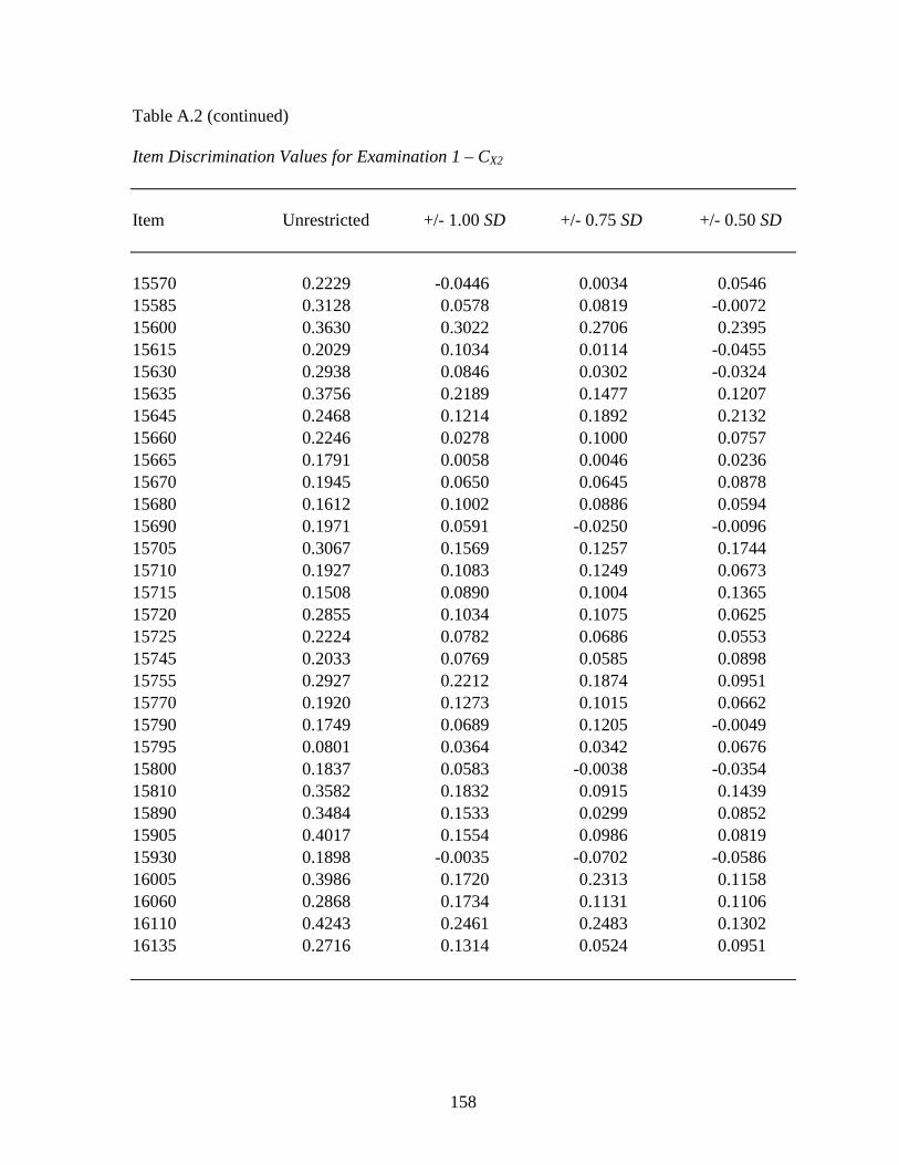
158
Table A.2 (continued) Item Discrimination Values for Examination 1 – CX2 Item Unrestricted +/- 1.00 SD +/- 0.75 SD +/- 0.50 SD 15570 0.2229 -0.0446 0.0034 0.0546 15585 0.3128 0.0578 0.0819 -0.0072 15600 0.3630 0.3022 0.2706 0.2395 15615 0.2029 0.1034 0.0114 -0.0455 15630 0.2938 0.0846 0.0302 -0.0324 15635 0.3756 0.2189 0.1477 0.1207 15645 0.2468 0.1214 0.1892 0.2132 15660 0.2246 0.0278 0.1000 0.0757 15665 0.1791 0.0058 0.0046 0.0236 15670 0.1945 0.0650 0.0645 0.0878 15680 0.1612 0.1002 0.0886 0.0594 15690 0.1971 0.0591 -0.0250 -0.0096 15705 0.3067 0.1569 0.1257 0.1744 15710 0.1927 0.1083 0.1249 0.0673 15715 0.1508 0.0890 0.1004 0.1365 15720 0.2855 0.1034 0.1075 0.0625 15725 0.2224 0.0782 0.0686 0.0553 15745 0.2033 0.0769 0.0585 0.0898 15755 0.2927 0.2212 0.1874 0.0951 15770 0.1920 0.1273 0.1015 0.0662 15790 0.1749 0.0689 0.1205 -0.0049 15795 0.0801 0.0364 0.0342 0.0676 15800 0.1837 0.0583 -0.0038 -0.0354 15810 0.3582 0.1832 0.0915 0.1439 15890 0.3484 0.1533 0.0299 0.0852 15905 0.4017 0.1554 0.0986 0.0819 15930 0.1898 -0.0035 -0.0702 -0.0586 16005 0.3986 0.1720 0.2313 0.1158 16060 0.2868 0.1734 0.1131 0.1106 16110 0.4243 0.2461 0.2483 0.1302 16135 0.2716 0.1314 0.0524 0.0951

159
Table A.2 (continued) Item Discrimination Values for Examination 1 – CX2 Item Unrestricted +/- 1.00 SD +/- 0.75 SD +/- 0.50 SD 16210 0.4188 0.2236 0.1434 0.0675 16255 0.1220 0.0794 0.0657 -0.0292 16275 0.1715 0.0896 0.0159 0.0851 16280 0.2719 0.1383 0.1093 0.0597 16305 0.1803 0.1924 0.1786 0.1146 16375 0.3525 0.0394 0.0232 0.0078 16390 0.2068 0.1290 0.2056 0.1613 16415 0.2210 0.0584 0.0624 0.0207 16425 0.2634 0.1260 0.0707 0.0361 16435 0.1672 0.1614 0.1378 0.0567 16445 0.2965 0.0898 0.1567 0.1322 16470 0.2230 0.0764 0.0099 -0.0402 16475 0.2791 0.1014 0.0883 -0.0315 16505 0.1442 0.0937 0.1442 0.1762 16515 0.1771 0.0177 0.0448 0.0582 16525 0.0557 -0.0036 0.0038 -0.0414 16560 0.2017 0.0466 -0.0084 -0.0655 16605 0.0227 0.0125 -0.0608 -0.0332 16615 0.2484 0.2078 0.1635 0.2102 16635 0.2581 0.0308 0.0928 0.1026 16690 0.3027 0.1090 0.0563 -0.0667 16710 0.4226 0.2040 0.1681 0.1408 16715 0.2471 0.1422 0.1150 0.1434 16720 0.4695 0.2503 0.1414 0.1803 16725 0.3359 0.2414 0.2626 0.3158 16740 0.3407 0.2174 0.1859 0.1624 16745 0.2644 0.1664 0.1095 0.0237 16755 0.2363 0.1324 0.0804 0.0205 16760 0.3060 0.1280 0.0616 0.0772 16765 0.3531 0.1070 0.1658 0.0452 16775 0.2067 0.1953 0.1598 0.1111

160
Table A.2 (continued) Item Discrimination Values for Examination 1 – CX2 Item Unrestricted +/- 1.00 SD +/- 0.75 SD +/- 0.50 SD 16800 0.2626 0.1244 0.0672 0.0886 16840 0.3550 0.1205 0.0740 0.1393 16845 0.4353 0.2553 0.2359 0.1161 16895 0.1322 0.0840 0.1307 0.0133 16910 0.3609 0.1927 0.1711 0.1150 16925 0.1134 0.0861 0.0643 -0.0075 16940 0.2813 0.1650 0.1874 0.1787 16945 0.2289 0.0630 0.0561 0.0568 16955 0.1375 0.1054 0.0855 0.1842 17010 0.2586 0.1811 0.0927 0.1929 17020 0.2144 0.1732 0.2085 0.1049 17050 0.1092 0.0615 0.0402 0.0376 17105 0.2338 0.0115 -0.0374 -0.1434 17115 0.2431 0.0537 0.0021 -0.0409 17125 0.1825 0.0764 0.0543 0.1113 17130 0.1915 0.1151 0.0356 0.1070 17160 0.0628 0.0838 0.0327 0.1226 17240 0.3277 0.1606 0.1184 0.1620 17245 0.2662 0.1052 0.0500 0.1546 17265 0.2291 0.1357 0.0975 -0.0071 17275 -0.0524 0.0646 0.0011 0.0113 17285 0.2758 0.1682 0.0747 0.1061 17300 0.1741 0.0590 0.0163 0.0228 17335 0.2070 0.0273 0.0675 0.0237 17340 0.1773 0.1121 0.1105 0.0678 17345 0.2649 0.1634 0.1149 0.1454 17370 0.3665 0.1842 0.1675 0.1755 17380 0.1734 -0.0353 -0.1138 -0.0456 17385 0.2695 0.1344 0.1355 0.1609 17425 0.2585 0.0531 0.0496 0.0563 17430 0.3883 0.1584 0.0991 0.0306

Table A.2 (continued) Item Discrimination Values for Examination 1 – CX2 Item Unrestricted +/- 1.00 SD +/- 0.75 SD +/- 0.50 SD 17460 0.2122 0.1120 0.0464 -0.0266 17480 0.2261 0.1542 0.1835 0.0457 17495 0.2081 0.0552 0.0452 0.0304 17500 0.3347 0.0832 -0.0147 -0.0760 17510 0.1919 0.1132 0.1074 0.1114 17520 0.1498 0.0951 0.1224 0.0837 17545 0.1543 0.0670 0.0068 0.0042 17550 0.0717 0.0530 0.0438 -0.0259 17565 0.1601 0.0825 0.0376 -0.0162 17580 0.3078 0.1566 0.1538 0.0810 17585 0.2006 0.0210 0.0300 0.0568 17595 0.2681 0.0957 0.0331 0.0731 17605 0.1571 0.0630 0.1039 0.0287 17635 0.1269 0.0557 0.0104 -0.0463 17640 0.2316 0.0753 0.0795 0.0011 17660 0.1847 0.1462 0.1284 0.1978 17665 0.2484 0.0991 0.0800 0.0288 17670 0.2394 0.1490 0.1667 0.2151 17690 0.1535 0.0732 0.1231 0.1294 17695 0.1150 0.0312 0.0880 0.0903
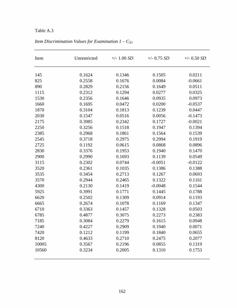
162
Table A.3 Item Discrimination Values for Examination 1 – CX3 Item Unrestricted +/- 1.00 SD +/- 0.75 SD +/- 0.50 SD 145 0.1624 0.1346 0.1505 0.0211 825 0.2558 0.1676 0.0084 -0.0661 890 0.2829 0.2156 0.1649 0.0511 1115 0.2312 0.1294 0.0277 0.0325 1530 0.2356 0.1646 0.0935 0.0973 1660 0.1695 0.0472 0.0200 -0.0537 1870 0.3104 0.1813 0.1239 0.0447 2030 0.1547 0.0516 0.0056 -0.1473 2175 0.3985 0.2342 0.1727 -0.0021 2250 0.3256 0.1518 0.1947 0.1394 2385 0.2968 0.1861 0.1564 0.1539 2545 0.3718 0.2975 0.2994 0.1919 2725 0.1192 0.0615 0.0868 0.0896 2830 0.3376 0.1953 0.1940 0.1470 2900 0.2990 0.1693 0.1139 0.0549 3115 0.2302 0.0744 -0.0051 -0.0122 3520 0.2361 0.1035 0.1386 0.1388 3535 0.3454 0.2713 0.1267 0.0693 3570 0.2944 0.2465 0.1322 0.1161 4300 0.2130 0.1419 -0.0048 0.1544 5925 0.3991 0.1771 0.1445 0.1788 6620 0.2502 0.1309 0.0914 0.1193 6665 0.2674 0.1078 0.1169 0.1347 6710 0.3363 0.1457 0.1328 0.0503 6785 0.4877 0.3075 0.2273 0.2383 7185 0.3084 0.2279 0.1615 0.0948 7240 0.4227 0.2909 0.1940 0.0071 7420 0.1212 0.1199 0.1840 0.0655 8120 0.4633 0.2710 0.2475 0.2077 10005 0.3567 0.2196 0.0855 0.1319 10560 0.3234 0.2005 0.1310 0.1753

163
Table A.3 (continued) Item Discrimination Values for Examination 1 – CX3 Item Unrestricted +/- 1.00 SD +/- 0.75 SD +/- 0.50 SD 10645 0.4002 0.2879 0.2730 0.3180 10690 0.1914 0.1130 0.0548 0.0196 11210 0.1892 0.0875 0.0586 -0.0204 11490 0.2190 0.0735 0.1106 0.1890 12530 0.2701 0.2103 0.1477 0.1876 12585 0.2238 0.0834 0.0909 0.1323 12770 0.2145 0.1828 0.1563 -0.0030 12895 0.3307 0.1737 0.0571 0.0795 12945 0.2775 0.0157 0.0199 0.0732 12960 0.3174 0.1701 0.1278 0.0726 12965 0.2288 0.1492 0.1777 0.0322 13020 0.2327 0.1367 0.0755 0.0275 13050 0.2285 0.1239 0.0878 -0.0187 13245 0.3465 0.2067 0.1887 0.1244 13500 0.2145 0.0503 0.0432 -0.0426 13695 0.2334 0.0990 0.0919 0.1156 14185 0.3771 0.2586 0.1969 0.1702 14275 0.3031 0.1733 0.1463 0.1158 15105 0.2166 0.0379 0.0021 0.0373 15145 0.1613 0.0918 0.0532 0.0959 15355 0.2608 0.1359 0.0582 0.0515 15395 0.2588 0.1882 0.1319 0.1348 15430 0.2713 0.2252 0.2117 0.1501 15450 0.4525 0.3004 0.2573 0.2423 15455 0.1563 0.0836 -0.0106 -0.0032 15500 0.1028 0.0428 -0.0104 -0.0050 15505 0.2527 0.1030 0.1357 -0.0001 15535 0.1162 0.1322 0.2029 0.2135 15540 0.2146 0.1791 0.1356 0.1005 15545 0.1930 0.0725 0.0836 -0.0788 15565 0.1988 0.1182 0.1608 0.0618

164
Table A.3 (continued) Item Discrimination Values for Examination 1 – CX3 Item Unrestricted +/- 1.00 SD +/- 0.75 SD +/- 0.50 SD 15570 0.2229 0.1422 0.0526 -0.0022 15585 0.3128 0.1837 0.1821 0.1162 15600 0.3630 0.2401 0.1280 0.0074 15615 0.2029 0.0485 0.0031 0.0773 15630 0.2938 0.1776 0.1562 0.1057 15635 0.3756 0.2724 0.2081 0.2122 15645 0.2468 0.0884 -0.0492 -0.2087 15660 0.2246 0.0785 0.0203 -0.0444 15665 0.1791 0.1022 0.0139 -0.0371 15670 0.1945 0.1314 0.0226 0.0533 15680 0.1612 0.0453 0.0824 0.0363 15690 0.1971 0.0686 0.1108 0.1018 15705 0.3067 0.1547 0.0816 0.0651 15710 0.1927 0.0966 0.0521 0.0785 15715 0.1508 -0.0171 -0.0966 -0.1205 15720 0.2855 0.1579 0.0953 0.0943 15725 0.2224 -0.0248 0.0199 0.0656 15745 0.2033 0.1265 0.0430 0.0023 15755 0.2927 0.1682 0.1694 0.0958 15770 0.1920 0.1560 0.0877 0.1448 15790 0.1749 0.0913 0.0494 0.0211 15795 0.0801 0.0511 0.0681 0.0131 15800 0.1837 0.1283 0.0506 0.0471 15810 0.3582 0.2133 0.2258 0.1557 15890 0.3484 0.2658 0.2478 0.1932 15905 0.4017 0.1553 0.1149 0.0867 15930 0.1898 0.0585 0.0869 0.0590 16005 0.3986 0.2270 0.1114 0.0222 16060 0.2868 0.1831 0.1302 0.0563 16110 0.4243 0.2460 0.2037 0.1184 16135 0.2716 0.1941 0.1827 0.1982

165
Table A.3 (continued) Item Discrimination Values for Examination 1 – CX3 Item Unrestricted +/- 1.00 SD +/- 0.75 SD +/- 0.50 SD 16210 0.4188 0.2911 0.2438 0.2194 16255 0.1220 0.0358 0.0782 0.0725 16275 0.1715 0.1281 0.1258 -0.0041 16280 0.2719 0.1301 0.0780 0.0783 16305 0.1803 0.1263 0.1301 0.0545 16375 0.3525 0.1110 0.0825 0.0262 16390 0.2068 0.0390 -0.0137 -0.0583 16415 0.2210 0.0901 0.0923 0.0524 16425 0.2634 0.0865 0.1162 0.0985 16435 0.1672 0.0272 -0.0071 0.0118 16445 0.2965 0.1442 0.0705 -0.0212 16470 0.2230 0.0794 0.0017 0.0833 16475 0.2791 0.1861 0.1934 0.1253 16505 0.1442 0.0919 0.0539 -0.0235 16515 0.1771 0.0268 0.0264 0.0213 16525 0.0557 -0.0013 -0.0689 -0.0472 16560 0.2017 0.0391 0.0512 0.0897 16605 0.0227 0.0615 0.0638 0.1439 16615 0.2484 0.1888 0.1556 0.0546 16635 0.2581 0.1022 0.1570 0.0523 16690 0.3027 0.2042 0.1332 0.2600 16710 0.4226 0.2303 0.1388 0.1003 16715 0.2471 0.0953 0.0719 0.0292 16720 0.4695 0.2956 0.2353 0.1531 16725 0.3359 0.2369 0.1568 -0.0343 16740 0.3407 0.2379 0.1548 0.0328 16745 0.2644 0.1473 0.1372 0.1648 16755 0.2363 0.1481 0.1060 0.1622 16760 0.3060 0.2510 0.1756 0.1428 16765 0.3531 0.2120 0.2155 0.0561 16775 0.2067 0.1021 0.0257 0.0668

166
Table A.3 (continued) Item Discrimination Values for Examination 1 – CX3 Item Unrestricted +/- 1.00 SD +/- 0.75 SD +/- 0.50 SD 16800 0.2626 0.0907 0.0811 -0.0197 16840 0.3550 0.1852 0.1166 0.0552 16845 0.4353 0.2708 0.2602 0.2084 16895 0.1322 0.0050 0.0198 0.0306 16910 0.3609 0.1964 0.1732 0.0960 16925 0.1134 0.0528 0.0117 0.1129 16940 0.2813 0.2190 0.1071 0.0342 16945 0.2289 0.1666 0.0282 0.0515 16955 0.1375 0.1039 0.0314 -0.0328 17010 0.2586 0.2377 0.1964 0.1457 17020 0.2144 0.1577 0.0304 0.0128 17050 0.1092 0.0639 0.0229 0.0292 17105 0.2338 -0.0110 0.0982 0.0896 17115 0.2431 0.1348 0.1411 0.1783 17125 0.1825 0.0728 0.0777 -0.0787 17130 0.1915 0.1616 0.1104 0.1207 17160 0.0628 0.0652 0.0363 0.0343 17240 0.3277 0.2360 0.1909 0.1432 17245 0.2662 0.0479 -0.0071 -0.0844 17265 0.2291 0.0967 0.1320 0.0842 17275 -0.0524 0.0094 0.0423 0.0198 17285 0.2758 0.1434 0.0236 0.1954 17300 0.1741 0.1414 0.0979 0.1365 17335 0.2070 0.1178 0.1094 -0.0308 17340 0.1773 0.1064 0.0692 0.0062 17345 0.2649 0.0987 0.0553 0.0084 17370 0.3665 0.1916 0.1137 -0.0362 17380 0.1734 0.0482 0.0789 0.0936 17385 0.2695 0.2846 0.1601 0.0807 17425 0.2585 0.1367 0.1224 0.0006 17430 0.3883 0.1833 0.1730 0.2077
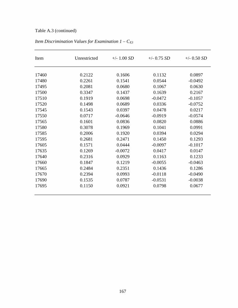
167
Table A.3 (continued) Item Discrimination Values for Examination 1 – CX3 Item Unrestricted +/- 1.00 SD +/- 0.75 SD +/- 0.50 SD 17460 0.2122 0.1606 0.1132 0.0897 17480 0.2261 0.1541 0.0544 -0.0492 17495 0.2081 0.0680 0.1067 0.0630 17500 0.3347 0.1437 0.1639 0.2167 17510 0.1919 0.0698 -0.0472 -0.1057 17520 0.1498 0.0689 0.0336 -0.0752 17545 0.1543 0.0397 0.0478 0.0217 17550 0.0717 -0.0646 -0.0919 -0.0574 17565 0.1601 0.0836 0.0820 0.0886 17580 0.3078 0.1969 0.1041 0.0991 17585 0.2006 0.1920 0.0394 0.0294 17595 0.2681 0.2471 0.1450 0.1293 17605 0.1571 0.0444 -0.0097 -0.1017 17635 0.1269 -0.0072 0.0417 0.0147 17640 0.2316 0.0929 0.1163 0.1233 17660 0.1847 0.1219 -0.0055 -0.0463 17665 0.2484 0.2351 0.1436 0.1286 17670 0.2394 0.0993 -0.0118 -0.0490 17690 0.1535 0.0787 -0.0531 -0.0038 17695 0.1150 0.0921 0.0798 0.0677

168
Table A.4 Item Discrimination Values for Examination 1 – CX4 Item Unrestricted +/- 1.00 SD +/- 0.75 SD +/- 0.50 SD 145 0.1624 0.0326 -0.0148 -0.1526 825 0.2558 0.0989 0.0995 0.0223 890 0.2829 0.1826 0.0656 -0.0168 1115 0.2312 0.1566 0.1577 -0.0331 1530 0.2356 0.1230 0.0857 0.0361 1660 0.1695 0.1765 0.1432 0.0252 1870 0.3104 0.1913 0.1340 0.0406 2030 0.1547 0.2095 0.2141 0.0772 2175 0.3985 0.2215 0.2183 0.1125 2250 0.3256 0.2215 0.1438 0.0924 2385 0.2968 0.0199 0.0457 0.0653 2545 0.3718 0.1682 0.0301 0.0339 2725 0.1192 0.1523 0.0794 0.0483 2830 0.3376 0.1354 0.1248 0.1792 2900 0.2990 0.2134 0.2401 0.1677 3115 0.2302 0.1251 0.0868 0.0360 3520 0.2361 0.1098 0.0516 0.1141 3535 0.3454 0.1755 0.1892 0.2181 3570 0.2944 0.2204 0.1468 0.0716 4300 0.2130 -0.0008 -0.0164 0.0485 5925 0.3991 0.1950 0.1332 0.0659 6620 0.2502 0.1430 0.2307 0.1934 6665 0.2674 0.1736 0.0968 0.1117 6710 0.3363 0.2705 0.2709 0.1515 6785 0.4877 0.3084 0.3131 0.2464 7185 0.3084 0.0519 0.0359 0.0461 7240 0.4227 0.2522 0.2483 0.1913 7420 0.1212 0.0309 -0.0616 -0.0992 8120 0.4633 0.2052 0.1759 0.1598 10005 0.3567 0.2582 0.2550 0.3006 10560 0.3234 0.1828 0.1661 0.1171

169
Table A.4 (continued) Item Discrimination Values for Examination 1 – CX4 Item Unrestricted +/- 1.00 SD +/- 0.75 SD +/- 0.50 SD 10645 0.4002 0.2247 0.1144 0.1737 10690 0.1914 0.0865 0.0868 0.1312 11210 0.1892 0.0950 0.1158 0.0745 11490 0.2190 0.1291 0.0534 0.0314 12530 0.2701 0.1152 0.1211 0.0226 12585 0.2238 0.1629 0.0876 0.0702 12770 0.2145 0.0470 0.0530 -0.0357 12895 0.3307 0.1939 0.1061 0.1345 12945 0.2775 0.1289 0.0393 0.0235 12960 0.3174 0.1474 0.0656 0.0221 12965 0.2288 0.2315 0.1989 0.0258 13020 0.2327 0.1748 0.1422 0.1041 13050 0.2285 0.1346 0.0928 0.0084 13245 0.3465 0.2104 0.1490 0.0086 13500 0.2145 0.0895 0.0723 0.1320 13695 0.2334 0.1971 0.1363 0.1890 14185 0.3771 0.2071 0.1970 0.0404 14275 0.3031 0.0758 0.0207 -0.0546 15105 0.2166 0.0867 0.0624 0.2087 15145 0.1613 0.0802 -0.0216 0.0456 15355 0.2608 0.2392 0.2147 0.2004 15395 0.2588 0.1788 0.1737 0.0870 15430 0.2713 0.1985 0.2224 0.1284 15450 0.4525 0.1934 0.1283 0.0415 15455 0.1563 0.1192 0.1431 0.1636 15500 0.1028 0.0939 0.0097 0.0435 15505 0.2527 0.0795 0.0139 -0.0478 15535 0.1162 0.0401 -0.0130 -0.1408 15540 0.2146 0.0461 -0.0226 0.0182 15545 0.1930 0.1047 0.0600 -0.1046 15565 0.1988 0.2201 0.1693 0.0799

170
Table A.4 (continued) Item Discrimination Values for Examination 1 – CX4 Item Unrestricted +/- 1.00 SD +/- 0.75 SD +/- 0.50 SD 15570 0.2229 0.0145 0.0041 -0.0543 15585 0.3128 0.0735 -0.0018 0.0000 15600 0.3630 0.3132 0.2843 0.2365 15615 0.2029 0.0596 0.0835 0.0352 15630 0.2938 0.1816 0.0571 0.0444 15635 0.3756 0.1656 0.1690 0.1239 15645 0.2468 0.1308 0.1781 0.2585 15660 0.2246 0.0899 0.0734 0.1176 15665 0.1791 0.0173 0.0245 0.0969 15670 0.1945 0.0503 0.0758 -0.0950 15680 0.1612 0.0898 0.0427 0.0655 15690 0.1971 0.0378 -0.0294 -0.0746 15705 0.3067 0.1783 0.1126 0.0072 15710 0.1927 0.0318 0.0625 0.0787 15715 0.1508 0.1717 0.1589 0.1383 15720 0.2855 0.1135 0.0532 -0.0533 15725 0.2224 0.1699 0.1259 0.0676 15745 0.2033 0.1261 0.0930 0.1045 15755 0.2927 0.2283 0.1541 0.0844 15770 0.1920 0.1359 0.0698 0.0827 15790 0.1749 0.0884 0.0410 0.0854 15795 0.0801 0.0866 0.0725 0.0490 15800 0.1837 0.0451 0.0457 0.0342 15810 0.3582 0.1834 0.1768 0.1241 15890 0.3484 0.1181 0.0717 0.1043 15905 0.4017 0.1452 0.1263 0.1024 15930 0.1898 0.0118 -0.0408 -0.0357 16005 0.3986 0.2598 0.1966 0.2944 16060 0.2868 0.1327 0.1664 0.1563 16110 0.4243 0.2512 0.1786 0.1798 16135 0.2716 0.0961 0.1020 0.0028

171
Table A.4 (continued) Item Discrimination Values for Examination 1 – CX4 Item Unrestricted +/- 1.00 SD +/- 0.75 SD +/- 0.50 SD 16210 0.4188 0.2581 0.1577 0.0892 16255 0.1220 0.0755 0.0294 0.0982 16275 0.1715 0.0469 0.1043 0.0235 16280 0.2719 0.1762 0.1021 0.0954 16305 0.1803 0.1073 0.1295 0.0779 16375 0.3525 0.0567 0.0484 0.1347 16390 0.2068 0.1706 0.1907 0.1594 16415 0.2210 0.0267 -0.0342 -0.1474 16425 0.2634 0.1207 0.0242 -0.0686 16435 0.1672 0.1233 0.1469 0.1668 16445 0.2965 0.1072 0.1003 0.1901 16470 0.2230 0.0575 0.0673 0.1140 16475 0.2791 0.0801 -0.0211 0.0101 16505 0.1442 0.0696 0.0840 -0.0990 16515 0.1771 0.1149 0.0150 -0.0221 16525 0.0557 -0.0293 0.0111 0.1407 16560 0.2017 0.0707 0.0525 0.0970 16605 0.0227 -0.0482 -0.0813 -0.1339 16615 0.2484 0.2189 0.1551 0.0330 16635 0.2581 0.1025 0.0448 0.1260 16690 0.3027 0.0897 0.0054 0.0294 16710 0.4226 0.2242 0.1518 0.1514 16715 0.2471 0.1497 0.1661 0.0755 16720 0.4695 0.2330 0.1807 -0.0017 16725 0.3359 0.3001 0.2878 0.1544 16740 0.3407 0.2449 0.2534 0.1767 16745 0.2644 0.0762 0.0717 0.1000 16755 0.2363 0.1424 0.0762 0.1414 16760 0.3060 0.1330 0.0617 -0.0266 16765 0.3531 0.1375 0.0923 0.0330 16775 0.2067 0.2230 0.2116 0.1678

172
Table A.4 (continued) Item Discrimination Values for Examination 1 – CX4 Item Unrestricted +/- 1.00 SD +/- 0.75 SD +/- 0.50 SD 16800 0.2626 0.0970 0.1628 0.1449 16840 0.3550 0.1149 0.1438 0.0094 16845 0.4353 0.2818 0.1781 0.0552 16895 0.1322 0.1844 0.0587 0.0493 16910 0.3609 0.2179 0.1848 0.1186 16925 0.1134 0.0928 0.0549 0.0370 16940 0.2813 0.1501 0.1416 0.2022 16945 0.2289 0.0514 0.0924 0.0836 16955 0.1375 0.1421 0.1383 0.1235 17010 0.2586 0.1345 0.1263 0.1055 17020 0.2144 0.2127 0.0890 0.1114 17050 0.1092 0.0616 0.0510 0.0330 17105 0.2338 0.0377 0.0050 -0.0116 17115 0.2431 0.0153 -0.0115 0.0248 17125 0.1825 0.0681 0.1069 0.0574 17130 0.1915 0.0582 0.1020 -0.0490 17160 0.0628 0.0169 0.1400 0.0906 17240 0.3277 0.1730 0.1492 0.1000 17245 0.2662 0.1353 0.1844 0.0125 17265 0.2291 0.1474 0.1439 0.0659 17275 -0.0524 0.0648 0.0543 -0.0377 17285 0.2758 0.2104 0.1706 0.1270 17300 0.1741 0.0287 0.0128 -0.0649 17335 0.2070 0.0732 0.0123 0.0053 17340 0.1773 0.0769 0.0959 0.1771 17345 0.2649 0.1441 0.1590 0.1065 17370 0.3665 0.1406 0.1705 0.1023 17380 0.1734 0.0088 -0.0375 -0.0472 17385 0.2695 0.1336 0.0970 -0.0600 17425 0.2585 0.0750 0.1044 0.1138 17430 0.3883 0.1796 0.1173 0.0529
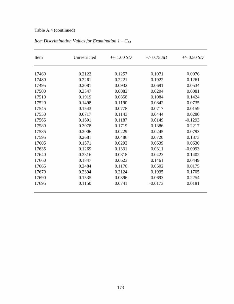
173
Table A.4 (continued) Item Discrimination Values for Examination 1 – CX4 Item Unrestricted +/- 1.00 SD +/- 0.75 SD +/- 0.50 SD 17460 0.2122 0.1257 0.1071 0.0076 17480 0.2261 0.2221 0.1922 0.1261 17495 0.2081 0.0932 0.0691 0.0534 17500 0.3347 0.0083 0.0204 0.0081 17510 0.1919 0.0858 0.1084 0.1424 17520 0.1498 0.1190 0.0842 0.0735 17545 0.1543 0.0778 0.0717 0.0159 17550 0.0717 0.1143 0.0444 0.0280 17565 0.1601 0.1187 0.0149 -0.1293 17580 0.3078 0.1719 0.1386 0.2217 17585 0.2006 -0.0229 0.0245 0.0793 17595 0.2681 0.0486 0.0720 0.1373 17605 0.1571 0.0292 0.0639 0.0630 17635 0.1269 0.1331 0.0311 -0.0093 17640 0.2316 0.0818 0.0423 0.1402 17660 0.1847 0.0623 0.1461 0.0449 17665 0.2484 0.1176 0.0502 0.0175 17670 0.2394 0.2124 0.1935 0.1705 17690 0.1535 0.0896 0.0693 0.2254 17695 0.1150 0.0741 -0.0173 0.0181

174
Table A.5 Item Discrimination Values for Examination 1 – CX5 Item Unrestricted +/- 1.00 SD +/- 0.75 SD +/- 0.50 SD 145 0.1624 0.0937 0.0477 0.0043 825 0.2558 0.1070 0.1200 0.0083 890 0.2829 0.1821 0.1828 0.1282 1115 0.2312 0.1220 0.0643 -0.2205 1530 0.2356 0.1158 0.1591 0.1251 1660 0.1695 0.1065 0.0543 -0.0052 1870 0.3104 0.1340 0.1337 0.0747 2030 0.1547 0.0205 -0.0362 -0.0914 2175 0.3985 0.2319 0.1610 0.1886 2250 0.3256 0.1481 0.0907 0.0973 2385 0.2968 0.2932 0.3219 0.2173 2545 0.3718 0.3704 0.2108 0.1134 2725 0.1192 -0.0093 0.0169 0.1191 2830 0.3376 0.1837 0.1528 0.2363 2900 0.2990 0.1169 0.1306 0.0451 3115 0.2302 0.0790 0.0377 -0.0131 3520 0.2361 0.1907 0.1368 0.0656 3535 0.3454 0.1666 0.1609 0.1436 3570 0.2944 0.1961 0.1219 0.0430 4300 0.2130 0.1235 0.1846 0.2335 5925 0.3991 0.2060 0.1819 0.0139 6620 0.2502 0.0796 0.1340 0.1647 6665 0.2674 0.1083 0.0794 0.0906 6710 0.3363 0.1231 0.1042 0.0503 6785 0.4877 0.2860 0.1998 0.1008 7185 0.3084 0.2583 0.2431 0.1661 7240 0.4227 0.2620 0.2692 0.1740 7420 0.1212 0.1857 0.1421 0.2106 8120 0.4633 0.3016 0.1914 0.1339 10005 0.3567 0.1271 0.1402 0.2053 10560 0.3234 0.1794 0.1085 -0.0038

175
Table A.5 (continued) Item Discrimination Values for Examination 1 – CX5 Item Unrestricted +/- 1.00 SD +/- 0.75 SD +/- 0.50 SD 10645 0.4002 0.3018 0.3006 0.1972 10690 0.1914 0.0847 0.0927 0.1487 11210 0.1892 0.0948 0.1104 0.1272 11490 0.2190 0.1160 0.0599 0.0020 12530 0.2701 0.2109 0.2589 0.1546 12585 0.2238 0.1639 0.0974 0.1202 12770 0.2145 0.1574 0.1738 0.1527 12895 0.3307 0.1083 0.0747 -0.0929 12945 0.2775 0.0790 0.0390 -0.0930 12960 0.3174 0.2051 0.1578 0.0107 12965 0.2288 0.1017 -0.0009 -0.0182 13020 0.2327 0.1016 0.0467 0.0452 13050 0.2285 0.1553 0.0751 -0.0046 13245 0.3465 0.2104 0.1377 0.0856 13500 0.2145 0.1285 0.0469 0.0859 13695 0.2334 0.0653 0.0760 0.1371 14185 0.3771 0.2524 0.2504 0.1490 14275 0.3031 0.2569 0.2617 0.1725 15105 0.2166 0.0078 0.1056 0.0568 15145 0.1613 0.0372 0.0484 -0.0455 15355 0.2608 0.0644 0.0536 0.1261 15395 0.2588 0.1652 0.1397 -0.0429 15430 0.2713 0.1773 0.0997 0.1382 15450 0.4525 0.3259 0.2216 0.1384 15455 0.1563 0.0191 0.0267 -0.0509 15500 0.1028 0.0125 0.0460 -0.0121 15505 0.2527 0.1576 0.0632 -0.0192 15535 0.1162 0.1978 0.1776 0.0291 15540 0.2146 0.1759 0.2321 0.2190 15545 0.1930 0.1097 0.0122 -0.0424 15565 0.1988 0.0411 -0.0041 0.0208

176
Table A.5 (continued) Item Discrimination Values for Examination 1 – CX5 Item Unrestricted +/- 1.00 SD +/- 0.75 SD +/- 0.50 SD 15570 0.2229 0.1718 0.1751 0.0885 15585 0.3128 0.2454 0.1973 0.2066 15600 0.3630 0.1857 0.1166 0.0643 15615 0.2029 0.0816 0.0534 -0.0131 15630 0.2938 0.2319 0.2168 0.1541 15635 0.3756 0.2302 0.1811 0.2114 15645 0.2468 -0.0099 -0.0395 0.0333 15660 0.2246 0.0640 0.0773 -0.0293 15665 0.1791 0.0625 0.1279 0.0858 15670 0.1945 0.1537 0.1587 -0.0291 15680 0.1612 0.0802 0.0233 -0.0080 15690 0.1971 0.1508 0.0750 0.0606 15705 0.3067 0.1803 0.0505 -0.0148 15710 0.1927 0.0747 0.0389 -0.0058 15715 0.1508 -0.0444 -0.0572 -0.1244 15720 0.2855 0.1780 0.1394 -0.0770 15725 0.2224 0.0661 0.0129 0.0175 15745 0.2033 0.0376 0.0823 0.0384 15755 0.2927 0.1555 0.0672 0.1272 15770 0.1920 0.0887 0.1453 0.0623 15790 0.1749 0.1648 0.1407 -0.0016 15795 0.0801 0.0082 0.0089 0.1319 15800 0.1837 0.1092 0.1324 0.1549 15810 0.3582 0.1756 0.1995 0.3237 15890 0.3484 0.2303 0.2419 0.3322 15905 0.4017 0.1764 0.1115 0.0534 15930 0.1898 0.0497 0.0123 0.1021 16005 0.3986 0.2210 0.1781 0.1658 16060 0.2868 0.1568 0.1513 0.1900 16110 0.4243 0.2521 0.1397 0.1144 16135 0.2716 0.2047 0.1587 0.2559

177
Table A.5 (continued) Item Discrimination Values for Examination 1 – CX5 Item Unrestricted +/- 1.00 SD +/- 0.75 SD +/- 0.50 SD 16210 0.4188 0.2665 0.2382 0.2047 16255 0.1220 0.0334 0.0502 0.0686 16275 0.1715 0.1114 0.1314 0.2231 16280 0.2719 0.1954 0.1277 0.0589 16305 0.1803 0.0598 -0.0017 -0.0005 16375 0.3525 0.1963 0.1123 0.1211 16390 0.2068 0.0928 -0.0340 -0.0618 16415 0.2210 0.1390 0.0576 0.0015 16425 0.2634 0.1116 0.0572 0.0461 16435 0.1672 0.0178 -0.0110 -0.0653 16445 0.2965 0.1245 0.0176 0.1032 16470 0.2230 0.0618 0.0810 0.0579 16475 0.2791 0.2140 0.1847 0.1152 16505 0.1442 0.0462 -0.0365 -0.1760 16515 0.1771 0.0099 -0.0570 -0.1010 16525 0.0557 -0.0421 -0.0165 0.0163 16560 0.2017 0.1201 0.1399 0.1473 16605 0.0227 0.1076 0.0658 0.0329 16615 0.2484 0.1331 0.0420 -0.0575 16635 0.2581 0.0779 0.0532 0.2335 16690 0.3027 0.2056 0.2417 0.1423 16710 0.4226 0.2604 0.1959 0.0423 16715 0.2471 0.1103 0.0889 -0.0341 16720 0.4695 0.3140 0.2672 0.0469 16725 0.3359 0.1690 0.0549 0.0522 16740 0.3407 0.2339 0.1416 0.0885 16745 0.2644 0.1573 0.1125 0.0156 16755 0.2363 0.1455 0.1299 0.0950 16760 0.3060 0.2325 0.2058 0.0681 16765 0.3531 0.2844 0.1999 0.1175 16775 0.2067 0.1370 0.0884 0.0113

178
Table A.5 (continued) Item Discrimination Values for Examination 1 – CX5 Item Unrestricted +/- 1.00 SD +/- 0.75 SD +/- 0.50 SD 16800 0.2626 0.0802 0.0606 0.1544 16840 0.3550 0.2071 0.1176 0.0611 16845 0.4353 0.2977 0.1702 0.0713 16895 0.1322 0.0347 -0.0619 -0.0933 16910 0.3609 0.2187 0.2064 0.0382 16925 0.1134 0.0449 0.0748 -0.0591 16940 0.2813 0.1512 0.1427 0.0582 16945 0.2289 0.0978 0.1447 0.0745 16955 0.1375 0.0253 0.0119 0.0192 17010 0.2586 0.1302 0.1414 0.1248 17020 0.2144 0.0608 0.0562 -0.0242 17050 0.1092 0.0501 0.0510 -0.0246 17105 0.2338 0.1698 0.1251 0.1069 17115 0.2431 0.1839 0.1494 0.1351 17125 0.1825 0.0658 0.0233 0.0365 17130 0.1915 0.1276 0.1095 0.0660 17160 0.0628 0.1016 0.1340 0.1322 17240 0.3277 0.2671 0.2135 0.1926 17245 0.2662 0.1124 -0.0107 -0.1466 17265 0.2291 0.1063 0.0837 0.1190 17275 -0.0524 -0.0694 -0.0494 0.0851 17285 0.2758 0.0835 0.1730 -0.0374 17300 0.1741 0.1673 0.1295 0.0307 17335 0.2070 0.1304 0.1133 0.1119 17340 0.1773 0.1290 0.1003 0.1004 17345 0.2649 0.0939 0.0689 -0.0474 17370 0.3665 0.1695 0.0389 0.1256 17380 0.1734 0.0917 0.1203 0.1460 17385 0.2695 0.2140 0.2053 0.1199 17425 0.2585 0.1435 0.1396 0.2140 17430 0.3883 0.2379 0.2515 0.0908
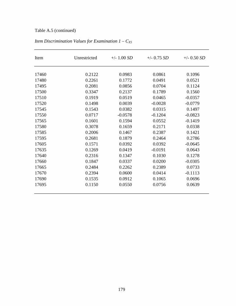
179
Table A.5 (continued) Item Discrimination Values for Examination 1 – CX5 Item Unrestricted +/- 1.00 SD +/- 0.75 SD +/- 0.50 SD 17460 0.2122 0.0983 0.0861 0.1096 17480 0.2261 0.1772 0.0491 0.0521 17495 0.2081 0.0856 0.0704 0.1124 17500 0.3347 0.2137 0.1789 0.1560 17510 0.1919 0.0519 0.0465 -0.0357 17520 0.1498 0.0039 -0.0028 -0.0779 17545 0.1543 0.0382 0.0315 0.1497 17550 0.0717 -0.0578 -0.1204 -0.0823 17565 0.1601 0.1594 0.0552 -0.1419 17580 0.3078 0.1659 0.2171 0.0338 17585 0.2006 0.1467 0.2387 0.1421 17595 0.2681 0.1879 0.2464 0.2786 17605 0.1571 0.0392 0.0392 -0.0645 17635 0.1269 0.0419 -0.0191 0.0643 17640 0.2316 0.1347 0.1030 0.1278 17660 0.1847 0.0337 0.0200 -0.0305 17665 0.2484 0.2262 0.2389 0.0733 17670 0.2394 0.0600 0.0414 -0.1113 17690 0.1535 0.0912 0.1065 0.0696 17695 0.1150 0.0550 0.0756 0.0639

180
APPENDIX B: ITEM DISCRIMINATION VALUES – EXAMINATION 2 Table B.1 Item Discrimination Values for Examination 2 – CX1 Item Unrestricted +/- 1.00 SD +/- 0.75 SD +/- 0.50 SD 32497 0.2411 0.1088 0.1045 0.3119 40655 0.3516 0.2677 0.2728 0.1453 40657 0.3651 0.1948 -0.1051 -0.0620 40668 0.3077 0.1417 0.1592 -0.0461 40885 0.4001 0.2015 -0.0435 -0.0805 40903 0.1012 0.0204 0.1016 0.0440 40907 0.0642 0.1555 0.1137 0.0939 40916 0.0227 0.1408 0.0667 0.0485 40944 0.2750 0.3059 0.2568 0.1897 40969 0.3391 0.3193 0.3707 0.3796 40992 0.3734 0.2826 0.1050 0.0509 41054 0.0845 -0.2002 -0.1794 -0.1965 41059 0.1457 0.1697 0.0926 0.1185 41066 0.0993 0.0626 0.1019 -0.1139 41093 0.2935 0.1386 -0.0086 0.0120 41098 0.1669 0.0264 0.1606 0.1545 41101 0.1742 0.1560 0.1077 0.0704 41181 0.3619 0.2595 0.1404 0.0876 41190 0.2607 0.1098 0.0807 0.0434 41337 0.1841 0.0721 -0.0447 0.1130 41407 0.2033 0.0772 0.1626 0.0524 41632 0.2642 0.1538 0.1429 0.2577 41645 0.2524 0.2612 0.0294 0.0234 41653 -0.0460 -0.0435 -0.0026 0.1456 41669 -0.0728 0.0051 0.0408 -0.0599 41690 0.1151 0.0477 -0.0077 0.0809 42503 0.2553 0.1759 0.0161 0.0337 42504 0.1333 -0.0408 -0.0308 -0.0690 51693 0.1997 0.1550 -0.0197 -0.1513

181
Table B.1 (continued) Item Discrimination Values for Examination 2 – CX1 Item Unrestricted +/- 1.00 SD +/- 0.75 SD +/- 0.50 SD 51717 0.1998 0.1537 0.2050 0.1044 51731 0.2534 0.0747 0.0125 0.0761 51732 0.1875 0.0388 0.0258 0.0063 51742 0.2057 -0.0932 0.0101 0.0495 51781 0.2811 0.2617 0.0883 0.1210 51786 0.1640 -0.0188 -0.1100 -0.0919 51787 0.3500 0.2684 0.1367 0.0703 51793 0.3382 0.1907 0.0770 0.0337 51806 0.3013 0.0783 0.1679 0.0776 51817 0.3639 0.1137 0.2227 0.1256 51825 0.2683 0.1417 0.0685 -0.0656 51839 0.0601 -0.1208 -0.0579 0.0741 51843 -0.0361 0.0095 -0.0785 -0.0844 59127 0.2984 0.0516 0.0607 0.0363 59128 0.2980 0.2535 0.1781 0.0248 59137 0.0786 0.1356 0.1849 0.0948 59138 0.1432 0.2705 0.1524 0.2133 59149 0.3560 0.1372 0.1294 -0.2314 59155 0.2243 0.1424 0.0573 -0.0345 59184 0.3020 0.1213 0.0784 0.0472 59185 0.0802 -0.0351 0.1374 0.1896 59217 0.1105 0.0538 0.0347 0.0000 59231 0.3649 0.1660 0.1124 0.1784 59239 0.2305 0.1372 0.2357 0.1786 59267 0.0877 0.1473 0.1972 0.2640 59489 0.2272 0.0358 0.0383 -0.0484 60230 0.2109 0.0000 0.0000 0.0000 60240 -0.0221 0.0692 0.1464 0.0743 60241 0.2474 -0.0835 -0.0642 -0.1499 60242 0.2856 0.3245 0.3093 0.0980 60250 0.1273 -0.0456 -0.0978 0.0058

182
Table B.1 (continued) Item Discrimination Values for Examination 2 – CX1 Item Unrestricted +/- 1.00 SD +/- 0.75 SD +/- 0.50 SD 60258 0.3100 0.3535 0.2324 0.1019 62125 0.1018 -0.1046 -0.0986 -0.1755 62129 0.2786 0.1223 0.1827 0.0713 62132 0.2708 0.2167 0.2131 0.2630 62135 0.2983 0.2064 0.2044 0.1020 62136 0.3512 0.2545 0.1068 0.1849 62140 0.3812 0.3175 0.3059 0.3243 84442 0.3069 0.3427 0.1779 -0.0328 90381 0.2819 0.1300 0.0799 0.0899 90382 0.0569 -0.0875 -0.0459 -0.0293 90384 0.1036 0.0280 0.1892 0.0765 90385 0.1792 0.0809 0.1522 0.0637 90386 0.2554 0.1521 0.1265 -0.0874 90390 0.4318 0.2788 0.1648 0.2544 90396 0.0718 -0.0149 -0.0912 0.0178 90397 0.1268 0.0301 -0.0399 -0.0980 90398 0.2795 0.2136 0.0011 0.1049 90400 0.1985 0.2581 0.0123 0.1101 94445 0.2217 0.0226 -0.1390 -0.2133 94505 0.0600 0.0874 0.1340 0.0115 94510 0.1683 0.1346 0.1603 0.1091 94566 0.3157 0.2505 0.1626 -0.0174 94582 0.3808 0.2083 0.1338 0.1438 94586 0.3209 0.1196 0.2029 0.1837 108131 0.1744 0.0693 -0.0800 -0.0696 108132 0.2818 0.1501 -0.0250 0.0891 108133 0.1783 0.1505 0.0895 0.2447 108134 0.2241 0.1205 -0.0060 0.1733 108135 0.0995 0.0123 0.0845 -0.0590 108136 0.2619 0.1431 0.1045 0.1717 108137 0.1924 0.1771 0.0000 0.0000

183
Table B.1 (continued) Item Discrimination Values for Examination 2 – CX1 Item Unrestricted +/- 1.00 SD +/- 0.75 SD +/- 0.50 SD 108138 0.3920 0.2342 0.2480 0.0839 108139 0.2255 0.0218 -0.1041 -0.1280 108140 0.1381 0.0705 0.0461 0.1769 108141 0.0964 0.0340 0.0788 -0.0748 108142 0.2794 0.1865 0.2009 0.3159 108143 0.4001 0.2367 0.3507 0.3147 108144 0.2980 0.2610 0.1608 0.0062 108145 0.1484 0.0735 0.1589 0.0191 108146 0.3033 0.1912 0.1364 0.2508 108147 0.1831 0.1061 0.0302 0.1849 108148 0.1280 -0.0378 -0.0804 -0.0306 108149 -0.0003 -0.0045 0.0284 0.0653 108150 0.1513 0.0746 -0.0432 0.0410 108151 0.1869 0.1356 0.0359 -0.0693 108152 0.3092 0.0667 0.0031 -0.0805 108153 0.4983 0.3633 0.3799 0.4009 108154 0.3769 0.2998 0.1842 0.3276 108155 0.3370 0.0562 -0.0211 -0.0402 108156 0.3039 0.1754 0.1458 0.0122 108157 0.2223 0.0730 0.1115 0.0094 108158 0.1994 0.2088 0.1896 0.1006 108159 0.0479 -0.0548 -0.1484 -0.2965 108160 -0.0783 -0.0242 0.0621 0.0586 108161 -0.0186 0.1302 0.2062 0.2870 108162 0.3128 0.2080 0.2559 0.2191 108163 0.2605 0.1741 0.2342 0.1667 108164 0.2834 0.0740 0.1866 0.1513 108165 -0.0191 -0.0032 -0.0881 -0.2013 108166 0.3038 0.1698 0.1245 0.0899 108167 0.3061 0.1468 0.2038 0.0708 108168 0.2278 0.0633 0.0661 0.0556

184
Table B.1 (continued) Item Discrimination Values for Examination 2 – CX1 Item Unrestricted +/- 1.00 SD +/- 0.75 SD +/- 0.50 SD 108169 -0.0768 -0.1679 -0.2659 -0.2630 108170 0.2778 0.1033 0.0900 -0.0708 108171 0.1082 0.1786 0.0758 -0.0466 108172 0.0626 -0.0366 -0.1741 -0.1177 108173 0.2470 0.1272 0.0804 0.1750 108174 0.1734 0.1075 0.0961 0.0436 108175 0.2533 0.1593 0.1923 0.1063 108176 0.3077 0.2271 0.0810 -0.0843 108177 0.3764 0.1448 0.0299 -0.1053 108178 0.4233 0.2727 0.2012 0.3035 108179 0.0484 0.0543 -0.0744 -0.0849 108180 0.3023 0.2710 0.1600 0.0839 108181 0.2335 0.0185 -0.0181 0.0219 108182 0.3435 0.1362 -0.0165 0.1017 108183 0.2177 0.0914 0.0733 0.0413 108184 0.2636 0.0996 0.1018 0.2895 108185 -0.2086 -0.1260 -0.1461 -0.0351 108186 -0.1053 0.0000 0.0000 0.0000 108187 0.2966 0.2967 0.1270 -0.0990 108188 0.2519 -0.0497 -0.1329 -0.1258 108189 0.3518 0.2523 0.3109 0.3695 108190 0.2102 0.1429 0.2029 0.0749 108191 0.2098 0.0961 0.1530 0.2026 108192 0.2053 -0.0515 -0.0028 0.0564 108193 0.2459 0.2312 0.2570 0.3014 108194 0.1967 0.1117 0.2363 0.1381 108195 0.1906 0.1138 0.0027 -0.0350 108196 0.2824 0.0755 0.0942 0.1752 108197 0.2556 0.2702 0.3184 0.2874 108198 0.2492 0.2751 0.0787 0.0761 108199 0.2099 0.0687 -0.0039 -0.0428

185
Table B.1 (continued) Item Discrimination Values for Examination 2 – CX1 Item Unrestricted +/- 1.00 SD +/- 0.75 SD +/- 0.50 SD 108200 0.1870 0.1260 -0.0356 -0.0658 108201 0.3032 0.1365 0.1140 -0.1432 108202 -0.0915 -0.1807 -0.1019 0.0059 108203 -0.0080 -0.0564 0.1211 0.1383 108204 0.3355 0.1726 0.1002 0.0644 108477 0.3690 0.3482 0.4438 0.2723 108478 0.2129 0.3464 0.2730 0.2179 108479 0.2899 0.2657 0.1506 0.1274 108480 0.1822 0.0239 -0.0250 -0.1625 108481 0.2634 0.2052 0.1571 0.0942 108482 0.2746 0.0001 0.2489 0.1444 108483 0.3192 -0.0554 0.0399 -0.0519 108484 0.2636 0.1011 0.0268 -0.0127 108485 0.1653 0.0840 0.1294 0.1474 108486 0.4052 0.3405 0.2698 0.2398 108487 0.3372 0.2292 0.1781 0.0484 108488 0.1810 0.2683 0.2115 0.1441 108489 0.3494 0.0874 -0.0482 0.0980 108490 0.1444 0.0790 0.0177 0.1201 108491 0.0475 0.1464 -0.0475 -0.0061 108492 0.4010 0.3024 0.2600 0.2214 108493 0.1714 0.0297 0.0171 -0.1620 108494 0.3177 0.2564 0.1706 0.0551 108495 0.1151 -0.0390 -0.0312 -0.1451 108497 0.2921 0.1930 0.0910 0.1558 108498 0.2975 0.0949 0.0201 0.1049 108499 0.2863 0.1820 0.0229 -0.0977 108500 0.1575 0.0487 0.1197 0.0636 108501 0.0743 0.1239 -0.0333 0.0121 108502 0.1566 0.2135 0.2387 0.2550 108503 0.1387 0.0435 0.1541 0.1523

186
Table B.1 (continued) Item Discrimination Values for Examination 2 – CX1 Item Unrestricted +/- 1.00 SD +/- 0.75 SD +/- 0.50 SD 108504 0.1001 0.1834 0.1075 0.1422 108505 0.2677 0.1163 0.0931 0.0825 108506 0.3136 0.1253 0.1246 0.3025 108507 0.3458 0.1827 0.1238 0.0908 108508 0.2697 0.1583 0.0758 0.1447 108509 0.3294 0.1003 0.1494 -0.0464 108510 0.1560 -0.0513 0.0152 0.0121 108511 0.0278 -0.1043 -0.0483 0.0000 108512 0.2234 0.2715 0.0935 -0.0300 108513 0.1451 0.0620 0.0312 0.0000 108514 0.2470 0.0962 0.0856 0.0532 108515 0.3178 0.2680 0.2600 0.1618 108523 0.1711 -0.0361 0.1494 0.0194 108524 0.1976 0.0928 -0.0181 0.0328 108525 0.0897 -0.0013 -0.0400 -0.1213 950671494 0.1338 0.0737 0.0980 0.1684

187
Table B.2 Item Discrimination Values for Examination 2 – CX2 Item Unrestricted +/- 1.00 SD +/- 0.75 SD +/- 0.50 SD 32497 0.2411 -0.0409 0.0356 -0.0685 40655 0.3516 0.2498 0.2038 0.2693 40657 0.3651 0.1337 0.1451 -0.0118 40668 0.3077 0.2367 0.1325 0.2305 40885 0.4001 0.2311 0.2103 0.1320 40903 0.1012 -0.0477 0.0340 0.2328 40907 0.0642 0.0797 0.1475 0.2394 40916 0.0227 0.1476 0.1755 0.0237 40944 0.2750 0.3149 0.2527 0.1175 40969 0.3391 0.2484 0.2221 0.1288 40992 0.3734 0.2332 0.2357 0.1442 41054 0.0845 0.0599 0.0627 0.0166 41059 0.1457 0.1110 0.1369 0.0000 41066 0.0993 -0.0005 -0.0411 0.2237 41093 0.2935 0.0780 0.1270 -0.0072 41098 0.1669 0.1128 0.1325 0.3057 41101 0.1742 0.0943 0.1219 0.2197 41181 0.3619 0.1092 0.1940 0.1671 41190 0.2607 0.1729 0.0972 0.1656 41337 0.1841 0.1587 0.1123 -0.1718 41407 0.2033 0.1377 -0.0203 0.1618 41632 0.2642 0.1378 0.2057 0.0311 41645 0.2524 0.1910 0.2203 0.1220 41653 -0.0460 -0.0469 -0.0151 -0.1590 41669 -0.0728 0.0416 0.0186 0.0985 41690 0.1151 0.0899 0.0636 -0.0829 42503 0.2553 0.1381 0.1459 0.0578 42504 0.1333 0.0049 0.0296 0.2842 51693 0.1997 0.1037 0.1195 0.0556 51717 0.1998 -0.0024 -0.0203 0.0625 51731 0.2534 0.1898 0.1635 0.1393
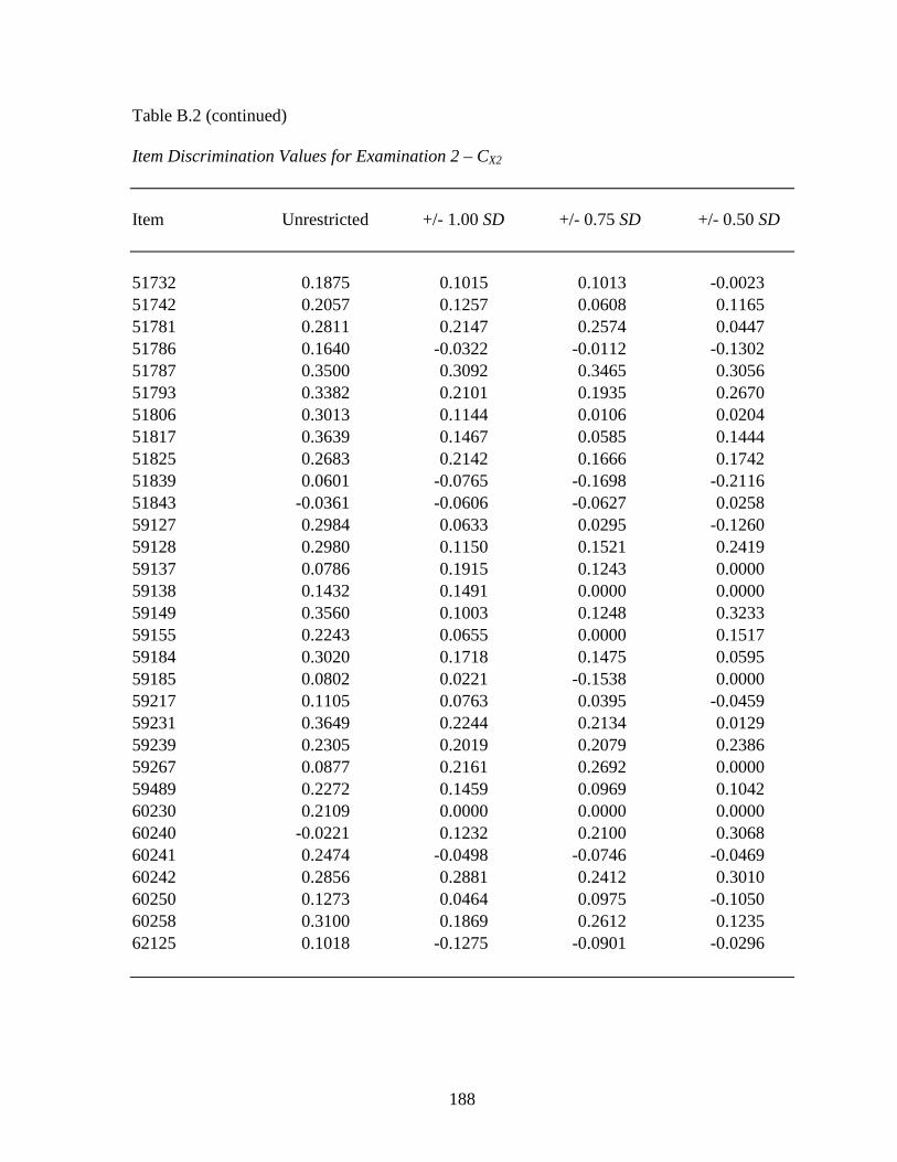
188
Table B.2 (continued) Item Discrimination Values for Examination 2 – CX2 Item Unrestricted +/- 1.00 SD +/- 0.75 SD +/- 0.50 SD 51732 0.1875 0.1015 0.1013 -0.0023 51742 0.2057 0.1257 0.0608 0.1165 51781 0.2811 0.2147 0.2574 0.0447 51786 0.1640 -0.0322 -0.0112 -0.1302 51787 0.3500 0.3092 0.3465 0.3056 51793 0.3382 0.2101 0.1935 0.2670 51806 0.3013 0.1144 0.0106 0.0204 51817 0.3639 0.1467 0.0585 0.1444 51825 0.2683 0.2142 0.1666 0.1742 51839 0.0601 -0.0765 -0.1698 -0.2116 51843 -0.0361 -0.0606 -0.0627 0.0258 59127 0.2984 0.0633 0.0295 -0.1260 59128 0.2980 0.1150 0.1521 0.2419 59137 0.0786 0.1915 0.1243 0.0000 59138 0.1432 0.1491 0.0000 0.0000 59149 0.3560 0.1003 0.1248 0.3233 59155 0.2243 0.0655 0.0000 0.1517 59184 0.3020 0.1718 0.1475 0.0595 59185 0.0802 0.0221 -0.1538 0.0000 59217 0.1105 0.0763 0.0395 -0.0459 59231 0.3649 0.2244 0.2134 0.0129 59239 0.2305 0.2019 0.2079 0.2386 59267 0.0877 0.2161 0.2692 0.0000 59489 0.2272 0.1459 0.0969 0.1042 60230 0.2109 0.0000 0.0000 0.0000 60240 -0.0221 0.1232 0.2100 0.3068 60241 0.2474 -0.0498 -0.0746 -0.0469 60242 0.2856 0.2881 0.2412 0.3010 60250 0.1273 0.0464 0.0975 -0.1050 60258 0.3100 0.1869 0.2612 0.1235 62125 0.1018 -0.1275 -0.0901 -0.0296

189
Table B.2 (continued) Item Discrimination Values for Examination 2 – CX2 Item Unrestricted +/- 1.00 SD +/- 0.75 SD +/- 0.50 SD 62129 0.2786 0.0722 0.0919 0.0699 62132 0.2708 0.2335 0.2262 0.0934 62135 0.2983 0.1945 0.2147 0.2990 62136 0.3512 0.2552 0.2120 -0.0235 62140 0.3812 0.2072 0.2383 0.1184 84442 0.3069 0.1904 0.1511 0.0700 90381 0.2819 0.2417 0.2833 0.1656 90382 0.0569 -0.0270 0.0174 0.0790 90384 0.1036 -0.0126 0.0568 0.2153 90385 0.1792 0.1035 -0.0138 -0.0617 90386 0.2554 0.0319 0.0816 0.1070 90390 0.4318 0.2446 0.1485 -0.0311 90396 0.0718 -0.0831 -0.2507 -0.3411 90397 0.1268 0.0316 -0.0064 0.1305 90398 0.2795 0.1817 0.1018 0.0740 90400 0.1985 0.1197 0.1070 0.0861 94445 0.2217 0.0171 -0.1217 -0.2287 94505 0.0600 0.0143 0.0634 -0.0759 94510 0.1683 0.1864 0.1453 0.0429 94566 0.3157 0.1226 0.0945 0.2292 94582 0.3808 0.1181 0.2256 0.1695 94586 0.3209 0.1981 0.2185 0.0121 108131 0.1744 0.0105 0.0207 0.0469 108132 0.2818 0.2602 0.2164 -0.0865 108133 0.1783 -0.0488 0.0032 -0.1045 108134 0.2241 0.1481 0.1232 0.0297 108135 0.0995 0.1083 0.1095 0.0279 108136 0.2619 0.1307 0.1885 0.1314 108137 0.1924 0.0000 0.0000 0.0000 108138 0.3920 0.3379 0.2430 0.2353 108139 0.2255 -0.1072 -0.0631 -0.0587

190
Table B.2 (continued) Item Discrimination Values for Examination 2 – CX2 Item Unrestricted +/- 1.00 SD +/- 0.75 SD +/- 0.50 SD 108140 0.1381 0.1324 0.0841 -0.0398 108141 0.0964 0.0539 0.0641 -0.0041 108142 0.2794 0.3282 0.3306 0.3337 108143 0.4001 0.2228 0.1770 -0.0022 108144 0.2980 0.2069 0.1486 -0.1215 108145 0.1484 0.0818 0.0727 0.0487 108146 0.3033 0.1245 -0.0142 -0.1655 108147 0.1831 0.1334 0.0434 -0.0895 108148 0.1280 -0.0283 -0.0687 -0.1046 108149 -0.0003 0.0193 0.0535 0.1319 108150 0.1513 0.1207 0.1502 0.2018 108151 0.1869 0.0852 0.0205 0.0903 108152 0.3092 0.0244 -0.0329 -0.0596 108153 0.4983 0.4318 0.3205 0.1534 108154 0.3769 0.3061 0.1561 0.0663 108155 0.3370 0.2068 0.0810 -0.0083 108156 0.3039 0.1962 0.1195 0.1964 108157 0.2223 0.1026 -0.0280 -0.0803 108158 0.1994 0.1983 0.1742 0.0972 108159 0.0479 -0.0009 -0.1028 -0.0762 108160 -0.0783 -0.0487 0.0139 -0.2239 108161 -0.0186 0.0268 0.0329 0.0000 108162 0.3128 0.2197 0.1607 -0.2268 108163 0.2605 0.1773 0.2176 0.1323 108164 0.2834 0.1937 0.1661 0.1679 108165 -0.0191 -0.0882 -0.1260 -0.0140 108166 0.3038 0.1974 0.1397 0.1454 108167 0.3061 0.2556 0.2492 0.1423 108168 0.2278 0.1328 0.1586 0.1722 108169 -0.0768 -0.1223 -0.0718 -0.0618 108170 0.2778 0.0695 0.1498 0.1763

191
Table B.2 (continued) Item Discrimination Values for Examination 2 – CX2 Item Unrestricted +/- 1.00 SD +/- 0.75 SD +/- 0.50 SD 108171 0.1082 0.0818 0.0882 0.0989 108172 0.0626 -0.0499 -0.1440 -0.2073 108173 0.2470 0.1050 0.0396 -0.1281 108174 0.1734 0.2191 0.2533 0.3011 108175 0.2533 0.2265 0.1590 0.1882 108176 0.3077 0.0356 0.0660 -0.0282 108177 0.3764 0.2775 0.1787 0.1763 108178 0.4233 0.2678 0.2430 0.1639 108179 0.0484 0.0942 0.0159 -0.0792 108180 0.3023 0.1829 0.1862 0.2005 108181 0.2335 0.1187 0.1325 0.0459 108182 0.3435 0.1400 0.0570 0.0145 108183 0.2177 0.0602 0.1471 0.1260 108184 0.2636 0.1966 0.0864 -0.0542 108185 -0.2086 -0.1775 -0.1737 -0.1801 108186 -0.1053 0.0000 0.0000 0.0000 108187 0.2966 0.0598 0.0906 0.1340 108188 0.2519 0.0627 -0.0230 -0.0222 108189 0.3518 0.2250 0.2959 0.0555 108190 0.2102 0.1048 0.0543 0.0845 108191 0.2098 0.0772 0.0848 0.0000 108192 0.2053 0.1652 0.0681 0.1117 108193 0.2459 0.2224 0.2608 0.0953 108194 0.1967 0.1120 0.0186 0.0079 108195 0.1906 0.1768 0.0788 -0.0568 108196 0.2824 0.0525 -0.0686 -0.0690 108197 0.2556 0.2288 0.2365 0.1443 108198 0.2492 0.2085 0.1556 0.1362 108199 0.2099 0.0962 -0.0188 0.0890 108200 0.1870 0.0545 0.0392 -0.0089 108201 0.3032 -0.0407 -0.1503 -0.0539

192
Table B.2 (continued) Item Discrimination Values for Examination 2 – CX2 Item Unrestricted +/- 1.00 SD +/- 0.75 SD +/- 0.50 SD 108202 -0.0915 -0.1957 -0.1736 -0.3521 108203 -0.0080 0.0047 -0.0679 0.0960 108204 0.3355 0.1792 0.2585 0.1443 108477 0.3690 0.3591 0.3629 0.2620 108478 0.2129 0.2162 0.3151 0.1808 108479 0.2899 0.1181 0.2497 0.2681 108480 0.1822 0.0954 -0.0510 -0.0046 108481 0.2634 0.2301 0.1354 0.0663 108482 0.2746 0.2312 0.1303 0.1886 108483 0.3192 0.1264 -0.0776 0.0314 108484 0.2636 0.1800 0.1125 0.1025 108485 0.1653 0.0653 0.0455 0.0918 108486 0.4052 0.2466 0.2064 0.0487 108487 0.3372 0.1526 0.1430 0.2869 108488 0.1810 0.1106 0.0996 0.1125 108489 0.3494 0.1799 0.1170 0.0214 108490 0.1444 0.1418 0.1149 -0.0248 108491 0.0475 0.0332 0.1788 -0.1105 108492 0.4010 0.1720 0.2435 0.1062 108493 0.1714 -0.0571 -0.0186 0.0519 108494 0.3177 0.1239 0.2521 0.0934 108495 0.1151 0.0337 -0.0012 0.0754 108497 0.2921 0.2791 0.1631 0.1070 108498 0.2975 0.2417 0.1986 0.0963 108499 0.2863 0.2217 0.0647 0.1240 108500 0.1575 0.1448 0.1184 0.1517 108501 0.0743 0.0221 -0.0156 -0.0257 108502 0.1566 0.1955 0.2897 0.1833 108503 0.1387 0.0786 0.0391 0.1912 108504 0.1001 0.1205 0.1496 0.0000 108505 0.2677 0.0018 -0.0048 -0.0092

193
Table B.2 (continued) Item Discrimination Values for Examination 2 – CX2 Item Unrestricted +/- 1.00 SD +/- 0.75 SD +/- 0.50 SD 108506 0.3136 0.2320 0.0521 -0.0286 108507 0.3458 0.3281 0.2820 0.2133 108508 0.2697 0.1885 0.2170 0.0453 108509 0.3294 0.1470 0.1566 0.3253 108510 0.1560 0.0060 -0.1199 -0.0163 108511 0.0278 0.1130 -0.0327 -0.0101 108512 0.2234 0.1716 0.0265 0.0830 108513 0.1451 0.0606 0.0599 -0.0522 108514 0.2470 0.1048 0.1871 0.1988 108515 0.3178 0.3673 0.3610 0.2085 108523 0.1711 0.0283 -0.0154 0.0738 108524 0.1976 0.0757 0.0732 0.0578 108525 0.0897 0.0051 0.0856 0.0429 950671494 0.1338 0.1032 0.1739 0.0523

194
Table B.3 Item Discrimination Values for Examination 2 – CX3 Item Unrestricted +/- 1.00 SD +/- 0.75 SD +/- 0.50 SD 32497 0.2411 0.1217 0.2911 0.2372 40655 0.3516 0.1787 0.1418 0.0946 40657 0.3651 0.1815 0.1862 -0.0338 40668 0.3077 0.0998 0.0199 -0.0814 40885 0.4001 0.0595 0.0126 -0.1389 40903 0.1012 0.1158 0.0044 -0.0519 40907 0.0642 0.0668 0.1101 0.0747 40916 0.0227 0.0482 0.0259 0.0198 40944 0.2750 0.1619 0.2943 0.0588 40969 0.3391 0.4393 0.3650 0.3248 40992 0.3734 0.1857 0.2219 0.1033 41054 0.0845 -0.2944 -0.4227 -0.3417 41059 0.1457 0.2378 0.1566 0.0467 41066 0.0993 0.1139 -0.0505 -0.0692 41093 0.2935 0.1475 0.0826 0.0153 41098 0.1669 -0.0142 -0.1313 -0.1752 41101 0.1742 0.0931 0.0579 0.1010 41181 0.3619 0.1822 0.2558 0.0544 41190 0.2607 0.1234 0.1521 -0.0783 41337 0.1841 0.0156 0.0357 0.0783 41407 0.2033 0.0939 0.2159 0.1236 41632 0.2642 0.1513 0.2437 0.1469 41645 0.2524 0.0773 0.1553 0.0205 41653 -0.0460 -0.0020 -0.1137 -0.0819 41669 -0.0728 -0.0029 0.0334 0.0506 41690 0.1151 0.1193 0.0190 0.1119 42503 0.2553 0.1045 0.0600 0.1416 42504 0.1333 -0.0560 -0.1206 -0.2483 51693 0.1997 0.0725 -0.0334 -0.0090 51717 0.1998 0.2391 0.3013 0.2927 51731 0.2534 -0.0200 -0.0325 -0.1187

195
Table B.3 (continued) Item Discrimination Values for Examination 2 – CX3 Item Unrestricted +/- 1.00 SD +/- 0.75 SD +/- 0.50 SD 51732 0.1875 -0.0100 -0.0683 0.0772 51742 0.2057 -0.1380 -0.1095 0.0286 51781 0.2811 -0.0394 0.0874 0.1686 51786 0.1640 0.0213 0.1243 0.1089 51787 0.3500 0.2230 0.0849 -0.0812 51793 0.3382 0.1669 0.0782 -0.1707 51806 0.3013 0.2396 0.1721 0.0234 51817 0.3639 0.1244 0.0426 0.2945 51825 0.2683 0.0962 -0.0146 -0.0276 51839 0.0601 0.1050 0.0366 0.0823 51843 -0.0361 -0.0055 0.0191 0.0283 59127 0.2984 0.0736 0.0298 0.0776 59128 0.2980 0.3114 0.1593 0.0617 59137 0.0786 0.0871 0.0980 0.1616 59138 0.1432 0.2311 0.2990 0.1532 59149 0.3560 0.1274 -0.1024 -0.1454 59155 0.2243 0.1461 0.0779 0.0567 59184 0.3020 0.0842 0.0433 0.0343 59185 0.0802 0.0670 0.0771 0.1266 59217 0.1105 0.1144 0.1114 0.0585 59231 0.3649 0.3284 0.0592 0.1412 59239 0.2305 0.1432 0.0148 -0.0674 59267 0.0877 0.0838 0.0872 0.1450 59489 0.2272 0.0759 -0.0345 -0.0298 60230 0.2109 0.2620 0.0000 0.0000 60240 -0.0221 0.0301 -0.0949 -0.0783 60241 0.2474 0.0609 -0.0407 -0.0979 60242 0.2856 0.1924 0.1850 0.1290 60250 0.1273 -0.1714 -0.1301 -0.0428 60258 0.3100 0.2502 0.3162 0.3900 62125 0.1018 -0.0626 -0.0799 -0.1394

196
Table B.3 (continued) Item Discrimination Values for Examination 2 – CX3 Item Unrestricted +/- 1.00 SD +/- 0.75 SD +/- 0.50 SD 62129 0.2786 0.2183 0.0703 0.1507 62132 0.2708 0.2230 0.1634 0.1714 62135 0.2983 0.1894 0.0622 -0.0243 62136 0.3512 0.0556 0.0980 0.0734 62140 0.3812 0.3997 0.2932 0.1867 84442 0.3069 0.2896 0.3430 0.2690 90381 0.2819 0.0743 0.0308 0.0544 90382 0.0569 -0.0666 -0.1631 -0.1797 90384 0.1036 0.0291 -0.0618 -0.1006 90385 0.1792 0.1182 0.0907 0.1984 90386 0.2554 0.2240 0.1738 0.0131 90390 0.4318 0.2296 0.3076 0.2261 90396 0.0718 0.0581 0.2216 0.2125 90397 0.1268 0.0539 0.0679 0.0027 90398 0.2795 0.1449 0.1014 0.0765 90400 0.1985 0.1838 0.2377 0.0545 94445 0.2217 0.0902 0.2386 0.2064 94505 0.0600 0.0758 0.2334 0.1571 94510 0.1683 0.2604 0.0842 0.2566 94566 0.3157 0.1853 0.1088 -0.0114 94582 0.3808 0.2727 0.2503 0.0715 94586 0.3209 0.1767 0.1205 0.0739 108131 0.1744 -0.0082 -0.0508 -0.1536 108132 0.2818 -0.0358 0.0473 0.0858 108133 0.1783 0.1990 0.2375 0.2328 108134 0.2241 0.0081 0.0877 0.0675 108135 0.0995 -0.0635 -0.0919 0.0243 108136 0.2619 0.0560 0.0854 0.0194 108137 0.1924 0.1588 0.2087 0.0000 108138 0.3920 0.1531 0.1059 0.1550 108139 0.2255 0.0048 0.1009 0.0857

197
Table B.3 (continued) Item Discrimination Values for Examination 2 – CX3 Item Unrestricted +/- 1.00 SD +/- 0.75 SD +/- 0.50 SD 108140 0.1381 0.0922 0.0667 0.0519 108141 0.0964 -0.1230 -0.0641 0.1657 108142 0.2794 0.1372 0.0225 -0.0360 108143 0.4001 0.2199 0.3057 0.3272 108144 0.2980 0.2069 0.3116 0.3302 108145 0.1484 0.1023 0.0881 0.1930 108146 0.3033 0.2080 0.3127 0.2948 108147 0.1831 0.1017 0.1227 0.0598 108148 0.1280 -0.0069 0.0870 0.0808 108149 -0.0003 0.0100 -0.1872 -0.1751 108150 0.1513 0.0463 0.0080 -0.2060 108151 0.1869 0.0749 0.0054 0.0814 108152 0.3092 -0.0013 0.0284 0.1362 108153 0.4983 0.3790 0.4198 0.2038 108154 0.3769 0.1944 0.2969 0.2564 108155 0.3370 -0.0389 -0.0162 0.0638 108156 0.3039 0.0818 0.1233 0.0519 108157 0.2223 0.1048 0.0668 0.2663 108158 0.1994 0.0958 0.0823 0.1313 108159 0.0479 -0.0489 -0.0332 -0.0308 108160 -0.0783 -0.0238 -0.0248 0.2878 108161 -0.0186 0.1776 0.2220 0.1996 108162 0.3128 0.2078 0.2890 0.3717 108163 0.2605 0.1899 0.1070 0.1781 108164 0.2834 0.2282 0.0387 -0.0213 108165 -0.0191 0.0059 0.0416 -0.0638 108166 0.3038 0.1530 0.0850 0.1153 108167 0.3061 -0.0156 -0.0932 0.1550 108168 0.2278 -0.0166 -0.0573 -0.0898 108169 -0.0768 -0.2375 -0.2086 -0.2323 108170 0.2778 0.1576 -0.0179 -0.0432

198
Table B.3 (continued) Item Discrimination Values for Examination 2 – CX3 Item Unrestricted +/- 1.00 SD +/- 0.75 SD +/- 0.50 SD 108171 0.1082 0.1928 0.2404 0.0388 108172 0.0626 0.0753 0.0234 0.0898 108173 0.2470 0.1042 0.2478 0.0885 108174 0.1734 -0.0273 -0.0603 -0.0777 108175 0.2533 0.1767 0.0518 0.0909 108176 0.3077 0.1837 0.2413 0.2623 108177 0.3764 0.1079 -0.0403 -0.1178 108178 0.4233 0.2860 0.1938 0.1592 108179 0.0484 0.1223 0.1089 -0.0271 108180 0.3023 0.2827 0.0541 0.0049 108181 0.2335 -0.1106 -0.1103 -0.1758 108182 0.3435 0.1203 0.1049 0.1034 108183 0.2177 0.0238 0.0199 0.0007 108184 0.2636 0.1160 0.1117 0.0898 108185 -0.2086 -0.0782 -0.0452 -0.1867 108186 -0.1053 -0.1932 -0.2581 0.0000 108187 0.2966 0.2050 0.3405 0.1056 108188 0.2519 -0.0577 -0.0594 -0.1239 108189 0.3518 0.2695 0.2531 0.2961 108190 0.2102 0.1495 0.0810 0.1066 108191 0.2098 0.2354 0.1738 0.1046 108192 0.2053 0.0072 -0.0668 -0.2116 108193 0.2459 0.2536 0.2892 -0.0176 108194 0.1967 0.1732 0.1037 0.3159 108195 0.1906 0.0752 0.0877 0.1234 108196 0.2824 0.2447 0.2598 0.1426 108197 0.2556 0.3347 0.3477 0.3605 108198 0.2492 0.0750 0.1668 0.1388 108199 0.2099 0.0096 0.0254 -0.0854 108200 0.1870 0.0532 0.1655 0.0288 108201 0.3032 0.2991 0.2748 0.3142

199
Table B.3 (continued) Item Discrimination Values for Examination 2 – CX3 Item Unrestricted +/- 1.00 SD +/- 0.75 SD +/- 0.50 SD 108202 -0.0915 -0.0465 0.0356 0.1872 108203 -0.0080 0.1403 0.0820 0.1054 108204 0.3355 0.0802 -0.0470 -0.1009 108477 0.3690 0.2985 0.1924 0.3385 108478 0.2129 0.2447 0.2236 0.3502 108479 0.2899 0.1261 0.1693 0.0900 108480 0.1822 -0.0022 -0.0028 -0.1547 108481 0.2634 0.1822 0.0962 0.2431 108482 0.2746 0.0888 -0.0717 -0.0044 108483 0.3192 0.0077 -0.0422 0.0113 108484 0.2636 0.0241 -0.0433 -0.1182 108485 0.1653 0.0430 -0.0136 0.0383 108486 0.4052 0.3345 0.4211 0.3361 108487 0.3372 0.2391 0.2514 -0.0842 108488 0.1810 0.3028 0.1783 0.0559 108489 0.3494 0.1110 0.0574 0.0238 108490 0.1444 0.0764 0.1009 0.1119 108491 0.0475 0.0339 0.0567 0.1032 108492 0.4010 0.2650 0.2272 0.1414 108493 0.1714 0.0953 0.0085 -0.0257 108494 0.3177 0.2071 0.1362 0.1086 108495 0.1151 0.0099 -0.0931 -0.1405 108497 0.2921 0.0552 0.0404 0.0257 108498 0.2975 0.0388 -0.0977 -0.1106 108499 0.2863 0.0663 0.0319 0.0551 108500 0.1575 0.0332 0.0608 -0.0183 108501 0.0743 0.1760 0.1984 0.0823 108502 0.1566 0.1520 0.1028 0.2247 108503 0.1387 0.1494 0.0831 -0.0423 108504 0.1001 0.1442 0.1800 0.0733 108505 0.2677 0.0876 0.1113 0.0872

200
Table B.3 (continued) Item Discrimination Values for Examination 2 – CX3 Item Unrestricted +/- 1.00 SD +/- 0.75 SD +/- 0.50 SD 108506 0.3136 0.1621 0.1950 0.1758 108507 0.3458 0.1042 0.0021 -0.0423 108508 0.2697 0.1154 0.0883 0.1295 108509 0.3294 0.1092 -0.0651 -0.1140 108510 0.1560 0.1441 0.0150 -0.0506 108511 0.0278 -0.0767 -0.1353 -0.0928 108512 0.2234 0.1574 0.1299 0.0605 108513 0.1451 0.0429 0.0230 0.0097 108514 0.2470 0.1620 0.0273 0.0174 108515 0.3178 0.1897 0.0232 0.1550 108523 0.1711 0.1200 -0.0043 0.0472 108524 0.1976 0.0942 0.1676 -0.0134 108525 0.0897 -0.1087 -0.1953 0.0201 950671494 0.1338 0.0129 0.0357 0.0349

201
Table B.4 Item Discrimination Values for Examination 2 – CX4 Item Unrestricted +/- 1.00 SD +/- 0.75 SD +/- 0.50 SD 32497 0.2411 -0.1008 -0.1401 -0.2282 40655 0.3516 0.2024 0.1856 0.0717 40657 0.3651 0.1839 0.1530 0.3669 40668 0.3077 0.2417 0.3198 0.1534 40885 0.4001 0.3218 0.4059 0.4472 40903 0.1012 0.0574 0.0744 -0.0954 40907 0.0642 0.1053 0.0294 -0.0912 40916 0.0227 0.0585 0.1114 0.2481 40944 0.2750 0.2208 0.2284 0.1060 40969 0.3391 0.1734 0.0080 -0.1036 40992 0.3734 0.2252 0.1796 0.3821 41054 0.0845 0.2010 0.2521 0.2333 41059 0.1457 0.1414 0.0000 0.0000 41066 0.0993 -0.0779 0.0920 0.0348 41093 0.2935 0.0969 0.1143 0.1182 41098 0.1669 0.1335 0.1465 -0.2560 41101 0.1742 0.1160 0.2201 0.1946 41181 0.3619 0.1414 0.1649 0.2030 41190 0.2607 0.1517 0.2625 0.1776 41337 0.1841 0.0847 0.0403 0.1182 41407 0.2033 0.0895 0.1256 -0.1482 41632 0.2642 0.1575 -0.0573 -0.1524 41645 0.2524 0.2136 0.1791 0.2934 41653 -0.0460 -0.0421 -0.1090 0.0049 41669 -0.0728 0.0424 -0.0025 0.1698 41690 0.1151 0.0430 0.0488 0.0249 42503 0.2553 0.1879 0.1130 0.1673 42504 0.1333 0.1102 0.1002 -0.1149 51693 0.1997 0.2041 0.1284 0.1210 51717 0.1998 -0.0286 -0.0828 -0.1889 51731 0.2534 0.1455 0.1492 0.1021

202
Table B.4 (continued) Item Discrimination Values for Examination 2 – CX4 Item Unrestricted +/- 1.00 SD +/- 0.75 SD +/- 0.50 SD 51732 0.1875 0.0911 0.1220 0.2345 51742 0.2057 0.1094 0.0485 0.1574 51781 0.2811 0.2842 0.1761 0.1674 51786 0.1640 -0.0971 -0.0056 0.0314 51787 0.3500 0.3534 0.3955 0.3739 51793 0.3382 0.1735 0.3432 0.3017 51806 0.3013 0.0307 0.1447 0.0063 51817 0.3639 0.1423 0.1080 -0.0523 51825 0.2683 0.3170 0.2920 0.2039 51839 0.0601 -0.1026 -0.1554 -0.0830 51843 -0.0361 -0.1070 -0.0823 0.0514 59127 0.2984 0.1170 0.0565 0.0433 59128 0.2980 0.1327 0.2331 0.1400 59137 0.0786 0.1313 0.0000 0.0000 59138 0.1432 0.0000 0.0000 0.0000 59149 0.3560 0.2238 0.2247 0.1428 59155 0.2243 -0.0026 0.0602 0.0473 59184 0.3020 0.1979 0.1827 0.2700 59185 0.0802 -0.0891 -0.0994 -0.1515 59217 0.1105 0.1360 0.0422 -0.0271 59231 0.3649 0.1058 0.1398 0.1596 59239 0.2305 0.1157 0.2070 -0.1744 59267 0.0877 0.1414 0.0000 0.0000 59489 0.2272 0.1015 0.1885 0.1037 60230 0.2109 0.0000 0.0000 0.0000 60240 -0.0221 0.1729 0.1333 0.1596 60241 0.2474 0.0201 0.0565 0.0173 60242 0.2856 0.2059 0.1876 0.1013 60250 0.1273 0.0859 0.0688 0.1171 60258 0.3100 0.0559 0.0115 0.2931 62125 0.1018 -0.0646 -0.0337 0.2210

203
Table B.4 (continued) Item Discrimination Values for Examination 2 – CX4 Item Unrestricted +/- 1.00 SD +/- 0.75 SD +/- 0.50 SD 62129 0.2786 0.0858 0.0622 -0.0131 62132 0.2708 0.1623 0.1133 0.1231 62135 0.2983 0.2405 0.1654 -0.0223 62136 0.3512 0.2524 0.1805 0.2300 62140 0.3812 0.1665 0.0158 0.0020 84442 0.3069 0.1943 0.0531 0.1410 90381 0.2819 0.2079 0.1367 0.1534 90382 0.0569 0.0482 0.0730 -0.0112 90384 0.1036 0.0004 0.0212 -0.0591 90385 0.1792 0.0780 -0.0655 -0.0012 90386 0.2554 0.1484 0.1108 0.0742 90390 0.4318 0.2234 0.1359 0.0163 90396 0.0718 -0.1581 -0.0904 -0.1955 90397 0.1268 0.0713 0.0313 -0.1344 90398 0.2795 0.1627 0.2002 0.1115 90400 0.1985 0.0562 0.1426 0.1210 94445 0.2217 -0.0389 -0.0144 0.0271 94505 0.0600 -0.0071 -0.0573 -0.1349 94510 0.1683 0.1897 0.0337 0.1053 94566 0.3157 0.1712 0.1686 0.1255 94582 0.3808 0.2002 0.0257 -0.0289 94586 0.3209 0.2932 0.1490 0.1285 108131 0.1744 -0.0416 0.0644 0.1593 108132 0.2818 0.3513 0.2107 0.3229 108133 0.1783 -0.0720 -0.1758 -0.1673 108134 0.2241 0.1065 0.0725 0.0061 108135 0.0995 0.2004 0.1655 0.1131 108136 0.2619 0.0481 0.0615 -0.0040 108137 0.1924 0.0000 0.0000 0.0000 108138 0.3920 0.2367 0.2288 0.1489 108139 0.2255 -0.0332 0.0412 0.1318
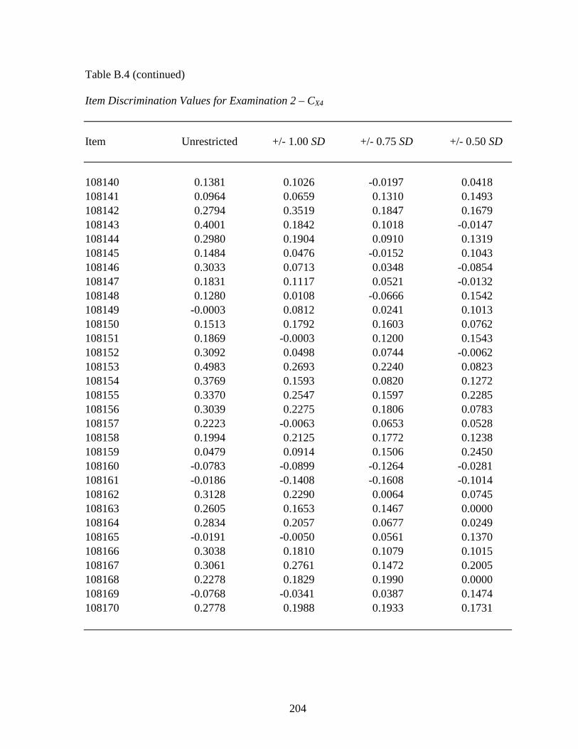
204
Table B.4 (continued) Item Discrimination Values for Examination 2 – CX4 Item Unrestricted +/- 1.00 SD +/- 0.75 SD +/- 0.50 SD 108140 0.1381 0.1026 -0.0197 0.0418 108141 0.0964 0.0659 0.1310 0.1493 108142 0.2794 0.3519 0.1847 0.1679 108143 0.4001 0.1842 0.1018 -0.0147 108144 0.2980 0.1904 0.0910 0.1319 108145 0.1484 0.0476 -0.0152 0.1043 108146 0.3033 0.0713 0.0348 -0.0854 108147 0.1831 0.1117 0.0521 -0.0132 108148 0.1280 0.0108 -0.0666 0.1542 108149 -0.0003 0.0812 0.0241 0.1013 108150 0.1513 0.1792 0.1603 0.0762 108151 0.1869 -0.0003 0.1200 0.1543 108152 0.3092 0.0498 0.0744 -0.0062 108153 0.4983 0.2693 0.2240 0.0823 108154 0.3769 0.1593 0.0820 0.1272 108155 0.3370 0.2547 0.1597 0.2285 108156 0.3039 0.2275 0.1806 0.0783 108157 0.2223 -0.0063 0.0653 0.0528 108158 0.1994 0.2125 0.1772 0.1238 108159 0.0479 0.0914 0.1506 0.2450 108160 -0.0783 -0.0899 -0.1264 -0.0281 108161 -0.0186 -0.1408 -0.1608 -0.1014 108162 0.3128 0.2290 0.0064 0.0745 108163 0.2605 0.1653 0.1467 0.0000 108164 0.2834 0.2057 0.0677 0.0249 108165 -0.0191 -0.0050 0.0561 0.1370 108166 0.3038 0.1810 0.1079 0.1015 108167 0.3061 0.2761 0.1472 0.2005 108168 0.2278 0.1829 0.1990 0.0000 108169 -0.0768 -0.0341 0.0387 0.1474 108170 0.2778 0.1988 0.1933 0.1731

205
Table B.4 (continued) Item Discrimination Values for Examination 2 – CX4 Item Unrestricted +/- 1.00 SD +/- 0.75 SD +/- 0.50 SD 108171 0.1082 0.1432 -0.0242 -0.0491 108172 0.0626 -0.0108 0.0098 0.0315 108173 0.2470 0.1681 0.1064 0.0085 108174 0.1734 0.3298 0.2310 0.1517 108175 0.2533 0.1238 0.2669 0.0738 108176 0.3077 0.0872 0.0308 0.1037 108177 0.3764 0.3003 0.3243 0.3186 108178 0.4233 0.2182 0.1827 0.0244 108179 0.0484 0.0225 0.0137 0.0565 108180 0.3023 0.2007 0.2488 0.1346 108181 0.2335 0.1870 0.1664 -0.0013 108182 0.3435 0.0929 0.0483 0.2210 108183 0.2177 0.1948 0.1532 0.1372 108184 0.2636 0.1513 0.1076 -0.0223 108185 -0.2086 -0.0682 -0.0959 -0.0743 108186 -0.1053 0.0000 0.0000 0.0000 108187 0.2966 0.0434 0.0980 0.1423 108188 0.2519 0.1026 0.1851 0.1029 108189 0.3518 0.1461 -0.0221 -0.0237 108190 0.2102 0.0417 0.0926 0.0042 108191 0.2098 0.1245 -0.0994 -0.1515 108192 0.2053 0.1081 0.1041 0.1860 108193 0.2459 0.2519 0.1430 -0.0174 108194 0.1967 0.0047 0.0553 -0.0362 108195 0.1906 0.0988 0.2072 0.1875 108196 0.2824 -0.1096 -0.0533 -0.2168 108197 0.2556 0.1955 0.0809 0.0991 108198 0.2492 0.1723 0.1878 0.1237 108199 0.2099 0.0955 0.1458 0.0711 108200 0.1870 0.1393 0.1453 0.0318 108201 0.3032 0.0130 0.0469 0.1239

206
Table B.4 (continued) Item Discrimination Values for Examination 2 – CX4 Item Unrestricted +/- 1.00 SD +/- 0.75 SD +/- 0.50 SD 108202 -0.0915 -0.1888 -0.3167 -0.1229 108203 -0.0080 -0.0621 -0.0586 -0.2977 108204 0.3355 0.1474 0.1512 0.1803 108477 0.3690 0.3697 0.1923 0.0364 108478 0.2129 0.2502 0.0510 0.3460 108479 0.2899 0.1500 0.1359 0.1131 108480 0.1822 0.1460 0.2189 0.0798 108481 0.2634 0.1928 0.2158 0.2609 108482 0.2746 0.2497 0.1659 -0.0067 108483 0.3192 0.1324 0.0978 -0.1615 108484 0.2636 0.1410 0.2098 0.1931 108485 0.1653 0.1035 0.0721 -0.0972 108486 0.4052 0.1651 0.0009 0.0768 108487 0.3372 0.2592 0.2063 -0.0056 108488 0.1810 0.0152 0.1042 0.0509 108489 0.3494 0.2902 0.1583 0.0959 108490 0.1444 0.1550 0.0959 0.1760 108491 0.0475 -0.0197 0.0221 0.1300 108492 0.4010 0.1912 0.0415 0.0000 108493 0.1714 -0.0034 0.0138 -0.0362 108494 0.3177 0.1256 0.0789 0.0951 108495 0.1151 0.0472 0.1000 0.0812 108497 0.2921 0.2616 0.1935 0.1212 108498 0.2975 0.3111 0.3042 0.2644 108499 0.2863 0.1936 0.3151 0.2911 108500 0.1575 0.0938 0.1467 0.0609 108501 0.0743 0.0325 -0.0553 -0.1424 108502 0.1566 0.2182 0.0242 0.1786 108503 0.1387 0.0240 0.0631 -0.0438 108504 0.1001 0.1514 0.0000 0.0000 108505 0.2677 0.0806 0.0379 -0.0597

207
Table B.4 (continued) Item Discrimination Values for Examination 2 – CX4 Item Unrestricted +/- 1.00 SD +/- 0.75 SD +/- 0.50 SD 108506 0.3136 0.2060 0.1717 -0.0784 108507 0.3458 0.2625 0.2849 0.1295 108508 0.2697 0.1941 0.1897 0.1565 108509 0.3294 0.1869 0.1687 0.0116 108510 0.1560 -0.0326 -0.0027 -0.1226 108511 0.0278 0.0907 0.0915 0.0325 108512 0.2234 0.1046 0.1938 0.0063 108513 0.1451 0.0370 0.0894 0.0517 108514 0.2470 0.0134 0.0654 0.0713 108515 0.3178 0.3937 0.2189 0.2571 108523 0.1711 -0.0392 -0.0464 -0.2090 108524 0.1976 0.1472 0.0412 -0.0318 108525 0.0897 -0.0182 0.0481 0.3214 950671494 0.1338 0.1095 0.0220 0.0102
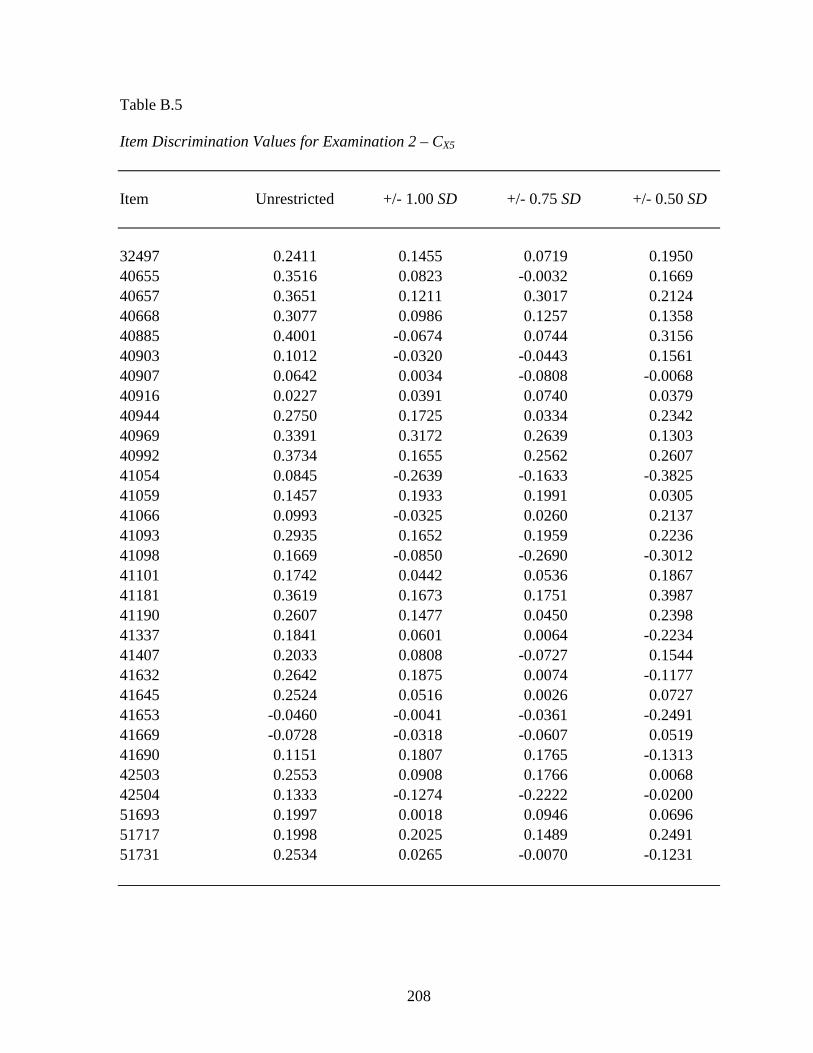
208
Table B.5 Item Discrimination Values for Examination 2 – CX5 Item Unrestricted +/- 1.00 SD +/- 0.75 SD +/- 0.50 SD 32497 0.2411 0.1455 0.0719 0.1950 40655 0.3516 0.0823 -0.0032 0.1669 40657 0.3651 0.1211 0.3017 0.2124 40668 0.3077 0.0986 0.1257 0.1358 40885 0.4001 -0.0674 0.0744 0.3156 40903 0.1012 -0.0320 -0.0443 0.1561 40907 0.0642 0.0034 -0.0808 -0.0068 40916 0.0227 0.0391 0.0740 0.0379 40944 0.2750 0.1725 0.0334 0.2342 40969 0.3391 0.3172 0.2639 0.1303 40992 0.3734 0.1655 0.2562 0.2607 41054 0.0845 -0.2639 -0.1633 -0.3825 41059 0.1457 0.1933 0.1991 0.0305 41066 0.0993 -0.0325 0.0260 0.2137 41093 0.2935 0.1652 0.1959 0.2236 41098 0.1669 -0.0850 -0.2690 -0.3012 41101 0.1742 0.0442 0.0536 0.1867 41181 0.3619 0.1673 0.1751 0.3987 41190 0.2607 0.1477 0.0450 0.2398 41337 0.1841 0.0601 0.0064 -0.2234 41407 0.2033 0.0808 -0.0727 0.1544 41632 0.2642 0.1875 0.0074 -0.1177 41645 0.2524 0.0516 0.0026 0.0727 41653 -0.0460 -0.0041 -0.0361 -0.2491 41669 -0.0728 -0.0318 -0.0607 0.0519 41690 0.1151 0.1807 0.1765 -0.1313 42503 0.2553 0.0908 0.1766 0.0068 42504 0.1333 -0.1274 -0.2222 -0.0200 51693 0.1997 0.0018 0.0946 0.0696 51717 0.1998 0.2025 0.1489 0.2491 51731 0.2534 0.0265 -0.0070 -0.1231

209
Table B.5 (continued) Item Discrimination Values for Examination 2 – CX5 Item Unrestricted +/- 1.00 SD +/- 0.75 SD +/- 0.50 SD 51732 0.1875 -0.0135 -0.0112 -0.1338 51742 0.2057 -0.0298 -0.0547 -0.2671 51781 0.2811 0.0174 -0.0498 -0.1169 51786 0.1640 0.1006 0.1758 0.2887 51787 0.3500 0.0307 0.0514 0.0918 51793 0.3382 0.1913 0.0589 0.3220 51806 0.3013 0.2184 0.1350 0.2362 51817 0.3639 0.1070 -0.0138 -0.0799 51825 0.2683 0.0376 0.1415 0.0465 51839 0.0601 0.0974 0.2371 -0.1575 51843 -0.0361 0.0486 0.1300 0.1934 59127 0.2984 0.2337 0.2855 0.0724 59128 0.2980 0.2475 0.3143 0.4245 59137 0.0786 0.0407 -0.0034 -0.0978 59138 0.1432 0.1859 0.1887 0.2717 59149 0.3560 -0.0121 0.0136 0.0514 59155 0.2243 0.1062 0.1666 0.3158 59184 0.3020 0.1532 0.1233 -0.0007 59185 0.0802 0.2104 0.0065 -0.0503 59217 0.1105 0.1335 0.0920 0.0503 59231 0.3649 0.2531 0.3572 -0.0034 59239 0.2305 0.1026 -0.0136 -0.0453 59267 0.0877 0.0245 -0.0407 -0.1959 59489 0.2272 0.1735 0.1705 -0.0683 60230 0.2109 0.2482 0.3083 0.0000 60240 -0.0221 -0.0886 -0.0543 -0.2751 60241 0.2474 0.0994 0.1165 0.0876 60242 0.2856 0.2061 0.0113 -0.0060 60250 0.1273 -0.0815 -0.1263 -0.2083 60258 0.3100 0.2682 0.3121 0.2751 62125 0.1018 -0.0414 0.2886 0.0513

210
Table B.5 (continued) Item Discrimination Values for Examination 2 – CX5 Item Unrestricted +/- 1.00 SD +/- 0.75 SD +/- 0.50 SD 62129 0.2786 0.1163 0.0594 0.0332 62132 0.2708 0.1170 0.0910 0.0404 62135 0.2983 0.0973 -0.0032 -0.0355 62136 0.3512 0.1218 0.1278 0.0089 62140 0.3812 0.2872 0.2699 0.1309 84442 0.3069 0.2408 0.2906 0.2346 90381 0.2819 0.1343 0.0455 -0.1277 90382 0.0569 -0.0280 -0.1320 -0.1776 90384 0.1036 -0.1136 -0.0726 -0.0088 90385 0.1792 0.1394 0.1804 -0.1209 90386 0.2554 0.2424 0.2017 0.3749 90390 0.4318 0.2959 0.1077 0.2671 90396 0.0718 0.0983 0.1217 0.3401 90397 0.1268 0.1249 -0.0422 0.1384 90398 0.2795 0.2431 0.1172 0.2108 90400 0.1985 0.1710 0.2266 0.2519 94445 0.2217 0.4427 0.3960 0.2101 94505 0.0600 0.0104 0.0461 0.1491 94510 0.1683 0.1729 0.2164 -0.1702 94566 0.3157 0.1377 0.0818 0.3680 94582 0.3808 0.2140 0.2818 0.1035 94586 0.3209 0.1527 0.2231 -0.1347 108131 0.1744 -0.0580 0.0130 0.0936 108132 0.2818 0.0460 0.0301 -0.1697 108133 0.1783 0.1810 0.1927 0.1170 108134 0.2241 0.1095 -0.0471 -0.1358 108135 0.0995 -0.1453 -0.2013 -0.1798 108136 0.2619 0.1840 0.0389 0.1430 108137 0.1924 0.1353 0.1485 0.2359 108138 0.3920 0.1862 0.0376 -0.1073 108139 0.2255 0.0782 0.0558 0.3834

211
Table B.5 (continued) Item Discrimination Values for Examination 2 – CX5 Item Unrestricted +/- 1.00 SD +/- 0.75 SD +/- 0.50 SD 108140 0.1381 0.1397 0.1336 -0.0994 108141 0.0964 -0.1663 -0.2452 -0.0174 108142 0.2794 0.0537 0.0016 -0.3701 108143 0.4001 0.1823 0.0062 0.1304 108144 0.2980 0.2150 0.2450 0.2240 108145 0.1484 0.1164 0.2684 -0.0231 108146 0.3033 0.2727 0.2381 0.1617 108147 0.1831 0.1680 0.2177 0.0757 108148 0.1280 0.1068 0.1711 0.1052 108149 -0.0003 -0.1253 -0.0344 -0.2881 108150 0.1513 0.0544 -0.0475 0.0453 108151 0.1869 0.0793 0.1865 0.2199 108152 0.3092 0.1057 0.0774 0.1876 108153 0.4983 0.4293 0.2363 0.0383 108154 0.3769 0.2079 0.2560 0.1708 108155 0.3370 0.0407 0.0878 -0.0478 108156 0.3039 0.0594 0.0192 0.0818 108157 0.2223 0.1718 0.2374 0.1191 108158 0.1994 -0.0082 0.0242 0.0505 108159 0.0479 -0.0006 0.1748 0.2690 108160 -0.0783 -0.0678 -0.0195 -0.2165 108161 -0.0186 0.1272 0.1053 0.1017 108162 0.3128 0.2670 0.1841 -0.0058 108163 0.2605 0.2152 0.1984 -0.0471 108164 0.2834 0.1596 0.1022 -0.1900 108165 -0.0191 0.0059 0.1772 0.2704 108166 0.3038 0.1606 0.0867 -0.1034 108167 0.3061 -0.0108 -0.0587 -0.2964 108168 0.2278 0.0519 -0.0140 -0.1576 108169 -0.0768 -0.2135 -0.2596 0.0000 108170 0.2778 0.0046 0.1606 0.2236

212
Table B.5 (continued) Item Discrimination Values for Examination 2 – CX5 Item Unrestricted +/- 1.00 SD +/- 0.75 SD +/- 0.50 SD 108171 0.1082 0.1585 0.0979 0.2359 108172 0.0626 0.0305 0.2162 0.0636 108173 0.2470 0.1637 0.0510 0.1172 108174 0.1734 0.0132 -0.0386 -0.2429 108175 0.2533 0.2820 0.1294 -0.0116 108176 0.3077 0.2464 0.2532 0.3877 108177 0.3764 0.1122 0.1671 0.0762 108178 0.4233 0.2682 0.1575 -0.0453 108179 0.0484 0.1551 0.1909 0.2500 108180 0.3023 0.1128 0.1259 0.2216 108181 0.2335 -0.1387 -0.1553 -0.2517 108182 0.3435 0.2730 0.3627 0.0859 108183 0.2177 -0.0041 -0.0407 0.0757 108184 0.2636 0.1495 0.0030 -0.0947 108185 -0.2086 0.0376 0.0944 0.1268 108186 -0.1053 -0.1729 -0.2018 -0.3433 108187 0.2966 0.3021 0.2034 0.4481 108188 0.2519 0.0393 0.0145 0.1430 108189 0.3518 0.3965 0.2078 -0.0877 108190 0.2102 0.0576 0.0461 0.2048 108191 0.2098 0.3791 0.2946 -0.0046 108192 0.2053 0.0340 0.0426 -0.1191 108193 0.2459 0.3143 0.0569 -0.1034 108194 0.1967 0.1171 0.0581 0.0936 108195 0.1906 0.1102 0.0937 0.2609 108196 0.2824 0.2942 0.3130 0.2000 108197 0.2556 0.3740 0.2885 0.0603 108198 0.2492 0.0932 0.0930 0.2470 108199 0.2099 0.0141 0.0305 0.2155 108200 0.1870 0.1277 0.0019 0.1978 108201 0.3032 0.2072 0.4069 0.6162

213
Table B.5 (continued) Item Discrimination Values for Examination 2 – CX5 Item Unrestricted +/- 1.00 SD +/- 0.75 SD +/- 0.50 SD 108202 -0.0915 0.0677 0.1483 -0.1814 108203 -0.0080 0.1077 0.0131 -0.0463 108204 0.3355 0.1143 0.0650 -0.0364 108477 0.3690 0.1987 0.0695 -0.2171 108478 0.2129 0.1263 0.1903 0.0529 108479 0.2899 0.1627 -0.0603 0.1299 108480 0.1822 -0.0225 -0.0153 0.2430 108481 0.2634 0.1603 0.2368 0.0637 108482 0.2746 0.0613 -0.0918 -0.3200 108483 0.3192 0.1574 0.0863 -0.1462 108484 0.2636 0.0333 0.0795 0.0660 108485 0.1653 0.0934 -0.0257 -0.0517 108486 0.4052 0.3243 0.2684 0.2781 108487 0.3372 0.1355 0.0561 0.3222 108488 0.1810 0.0763 0.1285 0.2950 108489 0.3494 0.1019 0.1679 -0.0158 108490 0.1444 0.0800 0.1511 -0.0007 108491 0.0475 0.1384 0.0872 0.0517 108492 0.4010 0.2368 0.2601 0.1209 108493 0.1714 0.0956 -0.0062 0.0907 108494 0.3177 0.0829 0.0058 0.1034 108495 0.1151 -0.0108 0.0846 0.0258 108497 0.2921 -0.0344 0.0610 -0.1084 108498 0.2975 0.0919 0.0699 -0.1491 108499 0.2863 0.0330 0.1719 0.2751 108500 0.1575 0.0747 0.0168 0.0024 108501 0.0743 0.0800 0.0890 0.1821 108502 0.1566 0.0288 0.0499 -0.1074 108503 0.1387 0.0232 0.1195 0.0837 108504 0.1001 0.1032 0.0852 0.0818 108505 0.2677 0.0584 0.0466 0.2470

214
Table B.5 (continued) Item Discrimination Values for Examination 2 – CX5 Item Unrestricted +/- 1.00 SD +/- 0.75 SD +/- 0.50 SD 108506 0.3136 0.2281 0.0231 0.0046 108507 0.3458 0.0471 -0.0836 -0.0818 108508 0.2697 0.2127 0.0012 -0.0088 108509 0.3294 -0.0356 -0.0054 -0.0198 108510 0.1560 0.1454 0.0394 0.0884 108511 0.0278 -0.1605 -0.2088 -0.2494 108512 0.2234 0.0308 0.1726 0.3128 108513 0.1451 -0.0312 0.0010 0.1075 108514 0.2470 0.1964 0.0910 -0.1871 108515 0.3178 0.0297 0.0407 -0.1912 108523 0.1711 0.2777 0.1268 -0.1705 108524 0.1976 0.2425 0.0819 0.0444 108525 0.0897 -0.1974 -0.0645 -0.1934 950671494 0.1338 0.0413 -0.1208 -0.1023
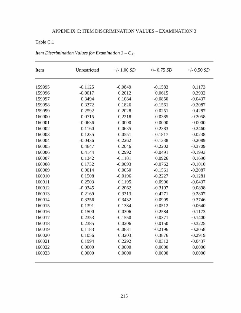
215
APPENDIX C: ITEM DISCRIMINATION VALUES – EXAMINATION 3 Table C.1 Item Discrimination Values for Examination 3 – CX1 Item Unrestricted +/- 1.00 SD +/- 0.75 SD +/- 0.50 SD 159995 -0.1125 -0.0849 -0.1583 0.1173 159996 -0.0017 0.2012 0.0615 0.3932 159997 0.3494 0.1084 -0.0850 -0.0437 159998 0.3372 0.1826 -0.1561 -0.2087 159999 0.2592 0.2028 0.0251 0.4287 160000 0.0715 0.2218 0.0385 -0.2058 160001 -0.0636 0.0000 0.0000 0.0000 160002 0.1160 0.0635 0.2383 0.2460 160003 0.1235 -0.0551 -0.1817 -0.0238 160004 -0.0436 -0.2262 -0.1338 0.2089 160005 0.4647 0.2046 -0.2202 -0.3709 160006 0.4144 0.2992 -0.0491 -0.1993 160007 0.1342 -0.1181 0.0926 0.1690 160008 0.1732 -0.0093 -0.0762 -0.1010 160009 0.0014 0.0050 -0.1561 -0.2087 160010 0.1508 -0.0196 -0.2227 -0.1281 160011 0.2503 0.1195 0.0996 -0.0437 160012 -0.0345 -0.2062 -0.3107 0.0898 160013 0.2169 0.3313 0.4271 0.2807 160014 0.3356 0.3432 0.0909 0.3746 160015 0.1391 0.1384 0.0512 0.0640 160016 0.1500 0.0306 0.2584 0.1173 160017 0.2353 -0.1550 0.0371 -0.1400 160018 0.2385 0.0206 0.0150 -0.3225 160019 0.1183 -0.0831 -0.2196 -0.2058 160020 0.1056 0.3203 0.3876 -0.2919 160021 0.1994 0.2292 0.0312 -0.0437 160022 0.0000 0.0000 0.0000 0.0000 160023 0.0000 0.0000 0.0000 0.0000

216
Table C.1 (continued) Item Discrimination Values for Examination 3 – CX1 Item Unrestricted +/- 1.00 SD +/- 0.75 SD +/- 0.50 SD 160024 -0.0251 0.1267 0.1364 0.1921 160025 0.1141 0.2719 0.4514 -0.0474 160026 0.1059 0.1562 0.1538 0.1852 160027 0.0230 0.0781 -0.3647 0.0000 160028 0.2308 0.1754 -0.0088 -0.0474 160029 0.3289 0.0913 -0.0694 0.0530 160030 0.2980 0.4566 0.2573 0.2460 160031 0.2154 0.1985 0.0854 -0.0808 160032 0.4353 0.2039 -0.0385 -0.0808 160033 -0.0930 0.0412 0.3579 0.5033 160034 0.4090 0.2046 0.1568 0.2682 160035 0.2824 0.2668 0.2755 0.3612 160036 0.0739 -0.0657 -0.2227 -0.4434 160037 -0.0380 0.0000 0.0000 0.0000 160038 0.0829 -0.0984 0.0766 0.0615 160039 0.1151 0.2090 0.1538 0.1852 160040 -0.0036 0.0346 0.3076 0.3103 160041 0.4053 0.3504 0.0736 -0.2260 160042 0.1553 -0.0364 -0.0921 -0.0474 160043 0.1101 0.0376 0.1957 0.2089 160044 0.1223 -0.0023 -0.1196 -0.0810 160045 0.1300 0.0532 0.2916 -0.0474 160046 0.2300 -0.1416 -0.0814 -0.0913 160047 0.1708 0.1643 -0.0187 -0.1139 160048 0.2581 0.1894 0.0461 -0.2260 160049 0.0586 -0.1206 -0.2200 -0.0056 160050 0.2836 0.4618 0.3757 0.0000 160051 0.3579 0.1745 0.0694 0.3136 160052 0.1241 0.0606 0.1066 -0.2044 160053 0.2348 0.2348 0.1290 0.4263 160054 0.1140 -0.0838 -0.0442 0.0640

217
Table C.1 (continued) Item Discrimination Values for Examination 3 – CX1 Item Unrestricted +/- 1.00 SD +/- 0.75 SD +/- 0.50 SD 160055 0.2920 0.2352 -0.0670 -0.3746 160056 0.2966 0.1313 0.2107 0.2751 160057 0.3838 0.2967 0.0563 -0.3330 160058 0.0012 -0.2917 0.0168 -0.0692 160059 0.2883 -0.1033 0.1318 0.0640 160060 0.0000 0.0000 0.0000 0.0000 160061 0.2186 -0.1030 0.2107 0.4535 160062 0.1056 -0.0701 -0.1561 -0.2087 160063 0.0365 0.0570 -0.0418 0.0898 160064 0.2481 0.3302 0.1592 -0.0441 160065 -0.0272 -0.2615 -0.4212 -0.1535 160066 -0.1009 0.0125 0.4269 0.2461 160067 0.0136 -0.0093 0.1637 0.0898 160068 0.0390 -0.1219 -0.2824 0.0000 160069 0.2224 -0.0120 0.2108 0.1364 160070 0.0423 -0.0533 0.3699 0.1921 160071 0.1943 0.0031 0.1559 -0.0810 160072 0.2186 0.2331 0.2169 0.2262 160073 0.2013 -0.0126 0.0217 0.3225 160074 0.3289 0.2292 -0.0088 0.0238 160075 0.0000 0.0000 0.0000 0.0000 160076 0.1443 -0.0093 0.0000 0.0000 160077 0.0059 0.1195 0.0703 -0.1281 160078 0.1822 -0.1186 -0.0921 0.4715 160079 0.3248 0.3558 0.0563 0.0808 160080 0.1056 -0.1063 -0.1862 0.4535 160081 0.1882 0.1195 0.1034 -0.1066 160082 0.1301 0.0649 0.3123 -0.0114 160083 0.1376 0.0823 0.2345 -0.2935 160084 0.2800 0.5687 0.3556 0.1139 160085 0.1580 -0.1030 -0.2944 0.0615

218
Table C.1 (continued) Item Discrimination Values for Examination 3 – CX1 Item Unrestricted +/- 1.00 SD +/- 0.75 SD +/- 0.50 SD 160086 0.1300 0.0572 0.3435 0.2044 160087 0.1955 0.0913 -0.2560 -0.1535 160088 -0.0804 -0.1961 -0.2351 -0.1998 160089 0.2772 0.0126 0.0619 0.4167 160090 -0.0300 0.1905 0.1637 0.0898 160526 0.2836 0.1977 0.2561 0.4535 160527 0.2211 0.1618 0.4232 0.0114 160528 0.1479 -0.0874 0.0038 -0.2919 160529 -0.0272 -0.2582 -0.2814 -0.2894 160530 0.1396 -0.0782 0.1867 0.2682 160531 0.1950 0.0346 -0.1162 0.1087 160532 0.0518 -0.0864 -0.2226 0.0000 160533 0.2074 0.1905 0.3911 0.1852 160534 0.0000 0.0000 0.0000 0.0000 160535 0.2356 0.4575 0.5232 0.3700 160536 0.0713 0.2292 0.1149 0.1377 160537 0.2885 0.1491 0.2862 0.6963 160538 0.1169 0.1491 -0.0533 -0.1535 160539 0.0901 0.1372 0.1034 0.2460 160540 0.1639 0.3961 0.3325 -0.0761 160541 0.3539 0.2337 -0.0217 0.0184 160542 0.1824 -0.1040 -0.0533 -0.1400 160543 0.0649 0.1152 0.2597 0.4715 160544 0.1833 -0.1929 0.0000 0.0000 160545 0.0954 0.1625 0.1385 0.1139 160546 0.0000 0.0000 0.0000 0.0000 160547 0.2811 0.0166 -0.1838 -0.1111 160548 0.2629 -0.0236 0.1241 0.1281 160549 0.2824 0.0992 0.0303 0.2807 160550 0.4042 0.1520 0.2144 -0.0471 160551 0.2205 0.0731 0.5155 0.5977

219
Table C.1 (continued) Item Discrimination Values for Examination 3 – CX1 Item Unrestricted +/- 1.00 SD +/- 0.75 SD +/- 0.50 SD 160552 0.3101 0.5026 0.2107 -0.1965 160553 0.1476 -0.0690 -0.0945 -0.3810 160554 0.2015 0.2326 0.2835 -0.0692 160555 0.3749 0.0000 0.0000 0.0000 160556 0.2813 0.0217 -0.1094 -0.1111 160557 0.3548 0.3032 0.0996 -0.0437 160558 0.2423 0.0606 -0.1316 0.0238 160559 0.2653 0.0290 -0.0088 -0.0474 160560 0.2133 0.0781 -0.0058 -0.3305 160561 0.2015 -0.2284 0.0000 0.0000 160562 -0.0636 0.0000 0.0000 0.0000 160563 0.1022 -0.0107 -0.1162 -0.1690 160564 0.2586 0.4015 0.2597 -0.1281 160565 0.1646 0.1414 0.1025 -0.1998 160566 0.2540 0.0478 0.1318 0.0898 160567 0.0320 -0.1033 -0.2558 -0.3873 160568 0.0281 0.1622 0.1962 0.3228 160569 0.2538 0.0063 0.1637 0.1852 160570 0.2961 0.1416 0.0312 -0.3330 160571 0.1201 -0.0584 -0.0736 0.1535 160572 0.2302 0.0584 0.0461 0.0332 160573 0.2998 -0.0015 -0.0251 -0.4287 160574 0.2106 -0.1929 0.0000 0.0000 160575 0.0609 0.1534 0.3550 0.1852 160576 0.0652 -0.1116 0.1558 0.1066 160577 0.1216 0.3236 0.1066 0.2058 160578 0.1544 0.1977 0.2561 0.4535

220
Table C.2 Item Discrimination Values for Examination 3 – CX2 Item Unrestricted +/- 1.00 SD +/- 0.75 SD +/- 0.50 SD 159995 -0.1125 -0.0180 -0.0655 -0.0555 159996 -0.0017 0.0173 -0.1121 0.1118 159997 0.3494 0.0504 -0.0360 -0.0488 159998 0.3372 0.2062 0.2302 0.1236 159999 0.2592 0.2640 0.1734 -0.0075 160000 0.0715 0.0223 0.2313 0.2765 160001 -0.0636 0.0000 0.0000 0.0000 160002 0.1160 0.2518 0.2922 0.2142 160003 0.1235 -0.1785 -0.1647 -0.2173 160004 -0.0436 -0.0804 -0.1274 -0.3181 160005 0.4647 0.0249 -0.0535 0.1118 160006 0.4144 0.1844 0.2643 0.3548 160007 0.1342 -0.1009 -0.1442 -0.1101 160008 0.1732 -0.0133 0.0817 0.0674 160009 0.0014 0.2062 0.2302 0.3368 160010 0.1508 0.2103 0.2298 0.3296 160011 0.2503 0.2637 0.2922 0.2550 160012 -0.0345 0.0886 0.0519 -0.2330 160013 0.2169 0.1471 -0.0657 0.2722 160014 0.3356 0.4352 0.4008 0.0674 160015 0.1391 0.1174 0.0888 -0.1277 160016 0.1500 0.0173 -0.1249 -0.1159 160017 0.2353 0.0488 -0.0664 0.0350 160018 0.2385 0.1029 0.1250 0.1416 160019 0.1183 -0.0727 0.0360 0.1861 160020 0.1056 -0.1309 -0.2356 0.2828 160021 0.1994 -0.0539 0.0841 0.0477 160022 0.0000 0.0000 0.0000 0.0000 160023 0.0000 0.0000 0.0000 0.0000 160024 -0.0251 -0.1067 0.0302 0.0000 160025 0.1141 0.1172 0.1028 0.1697

221
Table C.2 (continued) Item Discrimination Values for Examination 3 – CX2 Item Unrestricted +/- 1.00 SD +/- 0.75 SD +/- 0.50 SD 160026 0.1059 0.2839 0.3496 0.2722 160027 0.0230 0.0005 -0.0337 -0.1038 160028 0.2308 0.0482 -0.0029 -0.0824 160029 0.3289 0.1678 0.1261 -0.0360 160030 0.2980 0.2603 0.0137 0.1423 160031 0.2154 0.0522 0.2569 0.4330 160032 0.4353 0.2138 0.2906 0.2315 160033 -0.0930 -0.1229 -0.0952 -0.2416 160034 0.4090 0.2019 0.0608 0.1976 160035 0.2824 0.3741 0.3144 0.3932 160036 0.0739 0.0441 -0.0211 0.0154 160037 -0.0380 -0.2140 0.0000 0.0000 160038 0.0829 0.0478 0.0302 0.3487 160039 0.1151 0.1861 -0.0018 -0.0486 160040 -0.0036 0.0972 0.0259 -0.3030 160041 0.4053 0.1560 0.1443 0.1798 160042 0.1553 0.0727 0.0440 0.0098 160043 0.1101 0.2098 0.0753 0.2547 160044 0.1223 -0.2120 -0.0673 -0.0167 160045 0.1300 0.1483 0.1451 0.1697 160046 0.2300 0.1044 0.0372 -0.1179 160047 0.1708 0.1468 0.3210 0.4031 160048 0.2581 0.0140 0.0888 0.0674 160049 0.0586 0.0440 -0.0033 -0.1537 160050 0.2836 0.0000 0.0000 0.0000 160051 0.3579 0.3204 0.2585 -0.0797 160052 0.1241 0.1211 0.1915 0.0974 160053 0.2348 0.3454 0.1138 -0.1070 160054 0.1140 -0.1861 -0.2910 -0.4404 160055 0.2920 0.3076 0.3000 0.5385 160056 0.2966 0.2103 0.2298 -0.1531

222
Table C.2 (continued) Item Discrimination Values for Examination 3 – CX2 Item Unrestricted +/- 1.00 SD +/- 0.75 SD +/- 0.50 SD 160057 0.3838 0.3311 0.2519 0.3635 160058 0.0012 -0.0677 -0.1423 0.0619 160059 0.2883 0.1162 0.0841 0.0098 160060 0.0000 0.0000 0.0000 0.0000 160061 0.2186 -0.1268 -0.4155 -0.4807 160062 0.1056 0.1638 0.1663 0.2173 160063 0.0365 0.2251 0.2625 0.1171 160064 0.2481 0.0229 0.1588 0.1530 160065 -0.0272 -0.0146 -0.0052 -0.1346 160066 -0.1009 0.1454 0.1249 0.1159 160067 0.0136 -0.1268 0.0605 -0.1946 160068 0.0390 -0.0161 -0.0458 -0.1101 160069 0.2224 0.1801 0.0334 -0.0824 160070 0.0423 -0.1425 -0.2585 -0.3836 160071 0.1943 0.0014 0.0465 0.0828 160072 0.2186 0.3454 0.4090 0.3380 160073 0.2013 0.3213 0.1974 -0.0652 160074 0.3289 0.0413 -0.0380 0.1976 160075 0.0000 0.0000 0.0000 0.0000 160076 0.1443 -0.2085 -0.3414 -0.5215 160077 0.0059 -0.1271 0.0149 0.1179 160078 0.1822 -0.1752 -0.3759 -0.3580 160079 0.3248 0.3544 0.2830 0.2582 160080 0.1056 -0.0851 -0.2121 -0.2453 160081 0.1882 0.4100 0.4888 0.4336 160082 0.1301 -0.0660 0.0097 -0.1695 160083 0.1376 0.0424 0.1407 0.2765 160084 0.2800 0.1017 -0.0957 0.3380 160085 0.1580 -0.0851 -0.1800 -0.0719 160086 0.1300 0.0684 -0.0977 0.0555 160087 0.1955 0.1308 0.0935 0.0154

223
Table C.2 (continued) Item Discrimination Values for Examination 3 – CX2 Item Unrestricted +/- 1.00 SD +/- 0.75 SD +/- 0.50 SD 160088 -0.0804 -0.3558 -0.1655 0.0619 160089 0.2772 0.0621 0.0383 0.1261 160090 -0.0300 0.0693 0.2360 0.1171 160526 0.2836 0.2808 0.0000 0.0000 160527 0.2211 0.0629 0.0210 0.2315 160528 0.1479 -0.0851 -0.0241 -0.1199 160529 -0.0272 -0.1752 -0.0887 -0.0809 160530 0.1396 0.0272 0.0082 -0.1159 160531 0.1950 0.2776 0.2897 0.3688 160532 0.0518 0.0169 -0.0012 -0.0336 160533 0.2074 0.1035 0.0905 0.0619 160534 0.0000 0.0000 0.0000 0.0000 160535 0.2356 0.4433 0.4482 0.2668 160536 0.0713 0.1740 0.2568 0.3986 160537 0.2885 0.4596 0.3107 -0.1537 160538 0.1169 0.0318 0.0841 0.1798 160539 0.0901 0.0442 0.0587 -0.0694 160540 0.1639 0.0945 0.1164 0.2630 160541 0.3539 0.2127 0.0771 0.2198 160542 0.1824 0.0070 -0.1274 -0.1236 160543 0.0649 -0.0564 0.0243 -0.1101 160544 0.1833 -0.0821 -0.1348 -0.2630 160545 0.0954 0.1549 0.3949 0.1957 160546 0.0000 0.0000 0.0000 0.0000 160547 0.2811 0.0902 0.0259 0.0637 160548 0.2629 -0.0154 -0.1240 -0.3777 160549 0.2824 0.2642 0.3154 -0.0336 160550 0.4042 0.1331 0.1571 0.1256 160551 0.2205 0.1021 -0.0957 -0.0609 160552 0.3101 0.1894 0.2218 0.3380 160553 0.1476 0.0602 0.1309 0.0974

224
Table C.2 (continued) Item Discrimination Values for Examination 3 – CX2 Item Unrestricted +/- 1.00 SD +/- 0.75 SD +/- 0.50 SD 160554 0.2015 0.1488 0.1768 0.2722 160555 0.3749 0.0000 0.0000 0.0000 160556 0.2813 0.1544 0.1369 -0.0360 160557 0.3548 0.2098 0.2182 0.4002 160558 0.2423 0.1544 0.2661 0.0307 160559 0.2653 0.0617 0.1538 -0.0450 160560 0.2133 0.0478 0.0302 0.0066 160561 0.2015 -0.1151 -0.1793 0.0000 160562 -0.0636 0.0000 0.0000 0.0000 160563 0.1022 -0.0729 -0.0216 0.2615 160564 0.2586 0.2642 0.3154 0.2828 160565 0.1646 -0.0091 -0.0551 0.1171 160566 0.2540 0.1206 0.1138 0.0619 160567 0.0320 0.0440 -0.0033 -0.0926 160568 0.0281 0.2478 0.3104 0.0000 160569 0.2538 0.1172 -0.0724 -0.1946 160570 0.2961 0.1779 0.1588 0.1530 160571 0.1201 -0.0012 -0.2127 -0.2959 160572 0.2302 0.0752 0.1930 -0.1537 160573 0.2998 0.1286 -0.0445 0.0225 160574 0.2106 -0.0821 -0.1348 -0.2630 160575 0.0609 0.1861 -0.0018 -0.0486 160576 0.0652 0.0180 -0.0542 -0.0954 160577 0.1216 0.4867 0.4770 0.4420 160578 0.1544 0.2808 0.0000 0.0000
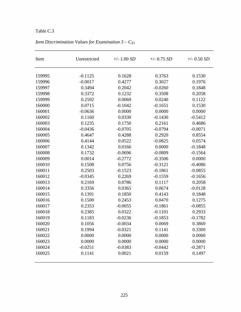
225
Table C.3 Item Discrimination Values for Examination 3 – CX3 Item Unrestricted +/- 1.00 SD +/- 0.75 SD +/- 0.50 SD 159995 -0.1125 0.1628 0.3763 0.1530 159996 -0.0017 0.4277 0.3027 0.1976 159997 0.3494 0.2042 -0.0260 0.1848 159998 0.3372 0.1232 0.3508 0.2058 159999 0.2592 0.0069 0.0240 0.1122 160000 0.0715 -0.1042 -0.1651 0.1530 160001 -0.0636 0.0000 0.0000 0.0000 160002 0.1160 0.0330 -0.1430 -0.5412 160003 0.1235 0.1750 0.2161 0.4686 160004 -0.0436 -0.0705 -0.0794 -0.0071 160005 0.4647 0.4288 0.2920 0.8554 160006 0.4144 0.0522 -0.0825 0.0574 160007 0.1342 0.0166 0.0000 -0.1848 160008 0.1732 -0.0696 -0.0809 -0.1564 160009 0.0014 -0.2772 -0.3506 0.0000 160010 0.1508 0.0756 -0.3121 -0.4086 160011 0.2503 -0.1523 -0.1861 -0.0855 160012 -0.0345 0.2269 -0.1559 -0.1656 160013 0.2169 0.0786 0.1117 0.2058 160014 0.3356 0.0365 0.0674 -0.0128 160015 0.1391 0.1850 0.4143 0.1848 160016 0.1500 0.2453 0.0470 0.1275 160017 0.2353 -0.0055 -0.1861 -0.0855 160018 0.2385 0.0322 -0.1101 0.2933 160019 0.1183 -0.0236 -0.1853 -0.1782 160020 0.1056 -0.0034 0.0069 0.3869 160021 0.1994 -0.0321 0.1141 0.3300 160022 0.0000 0.0000 0.0000 0.0000 160023 0.0000 0.0000 0.0000 0.0000 160024 -0.0251 -0.0383 -0.0442 -0.2871 160025 0.1141 0.0021 0.0159 0.1497
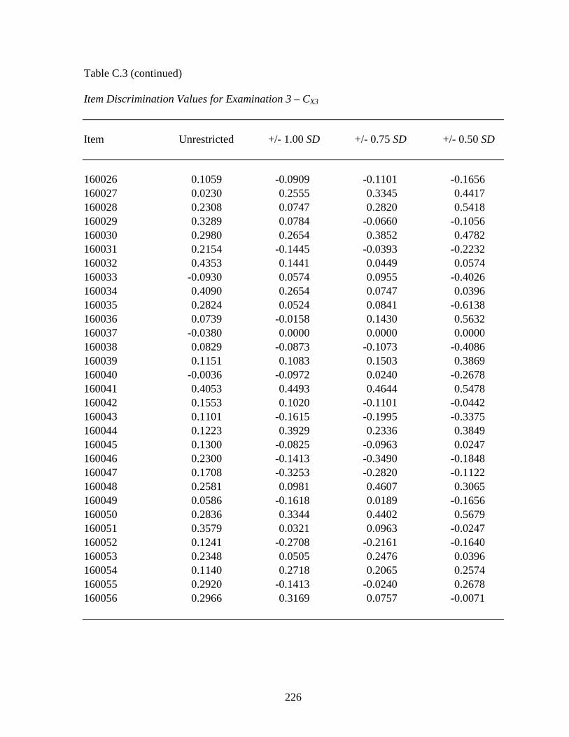
226
Table C.3 (continued) Item Discrimination Values for Examination 3 – CX3 Item Unrestricted +/- 1.00 SD +/- 0.75 SD +/- 0.50 SD 160026 0.1059 -0.0909 -0.1101 -0.1656 160027 0.0230 0.2555 0.3345 0.4417 160028 0.2308 0.0747 0.2820 0.5418 160029 0.3289 0.0784 -0.0660 -0.1056 160030 0.2980 0.2654 0.3852 0.4782 160031 0.2154 -0.1445 -0.0393 -0.2232 160032 0.4353 0.1441 0.0449 0.0574 160033 -0.0930 0.0574 0.0955 -0.4026 160034 0.4090 0.2654 0.0747 0.0396 160035 0.2824 0.0524 0.0841 -0.6138 160036 0.0739 -0.0158 0.1430 0.5632 160037 -0.0380 0.0000 0.0000 0.0000 160038 0.0829 -0.0873 -0.1073 -0.4086 160039 0.1151 0.1083 0.1503 0.3869 160040 -0.0036 -0.0972 0.0240 -0.2678 160041 0.4053 0.4493 0.4644 0.5478 160042 0.1553 0.1020 -0.1101 -0.0442 160043 0.1101 -0.1615 -0.1995 -0.3375 160044 0.1223 0.3929 0.2336 0.3849 160045 0.1300 -0.0825 -0.0963 0.0247 160046 0.2300 -0.1413 -0.3490 -0.1848 160047 0.1708 -0.3253 -0.2820 -0.1122 160048 0.2581 0.0981 0.4607 0.3065 160049 0.0586 -0.1618 0.0189 -0.1656 160050 0.2836 0.3344 0.4402 0.5679 160051 0.3579 0.0321 0.0963 -0.0247 160052 0.1241 -0.2708 -0.2161 -0.1640 160053 0.2348 0.0505 0.2476 0.0396 160054 0.1140 0.2718 0.2065 0.2574 160055 0.2920 -0.1413 -0.0240 0.2678 160056 0.2966 0.3169 0.0757 -0.0071

227
Table C.3 (continued) Item Discrimination Values for Examination 3 – CX3 Item Unrestricted +/- 1.00 SD +/- 0.75 SD +/- 0.50 SD 160057 0.3838 -0.0214 0.2625 0.4633 160058 0.0012 -0.1363 -0.1704 0.0000 160059 0.2883 0.2571 0.0159 -0.4280 160060 0.0000 0.0000 0.0000 0.0000 160061 0.2186 0.3752 0.4970 0.1152 160062 0.1056 -0.0298 -0.0275 0.0000 160063 0.0365 -0.1264 -0.1559 -0.1656 160064 0.2481 -0.0368 0.2359 0.4080 160065 -0.0272 -0.2933 -0.3714 -0.2871 160066 -0.1009 -0.1623 -0.0540 -0.5418 160067 0.0136 0.2337 0.3164 0.0247 160068 0.0390 0.0000 0.0000 0.0000 160069 0.2224 0.3586 0.1741 -0.0071 160070 0.0423 0.0863 0.1192 -0.0658 160071 0.1943 0.0069 0.0240 0.3849 160072 0.2186 0.0752 -0.2383 -0.4776 160073 0.2013 0.0522 0.1011 -0.2574 160074 0.3289 0.1832 0.2640 0.3300 160075 0.0000 0.0000 0.0000 0.0000 160076 0.1443 0.4053 0.5319 0.7490 160077 0.0059 0.2571 0.0159 0.1497 160078 0.1822 0.3455 0.0275 -0.2469 160079 0.3248 0.1042 0.2959 -0.0128 160080 0.1056 0.4407 0.0821 -0.0442 160081 0.1882 -0.1942 -0.1125 -0.3375 160082 0.1301 -0.0684 0.0606 0.0829 160083 0.1376 -0.2921 -0.1189 -0.0574 160084 0.2800 0.4020 0.5509 0.7655 160085 0.1580 0.1217 0.1651 0.0247 160086 0.1300 -0.2251 -0.1516 -0.1122 160087 0.1955 0.3720 0.2048 0.3849

228
Table C.3 (continued) Item Discrimination Values for Examination 3 – CX3 Item Unrestricted +/- 1.00 SD +/- 0.75 SD +/- 0.50 SD 160088 -0.0804 -0.1852 -0.2335 0.0000 160089 0.2772 0.0841 -0.0449 -0.3634 160090 -0.0300 0.0193 0.0347 0.0247 160526 0.2836 0.3344 0.4402 -0.0442 160527 0.2211 0.1623 0.1990 -0.1497 160528 0.1479 -0.1289 0.0275 0.1988 160529 -0.0272 -0.3069 -0.3891 0.0000 160530 0.1396 -0.0418 -0.0359 -0.0829 160531 0.1950 -0.1032 -0.3144 -0.5412 160532 0.0518 0.0000 0.0000 0.0000 160533 0.2074 0.0490 0.0732 0.1152 160534 0.0000 0.0000 0.0000 0.0000 160535 0.2356 0.3365 0.2935 0.0000 160536 0.0713 -0.3692 -0.2279 -0.6184 160537 0.2885 0.3510 0.1759 -0.4782 160538 0.1169 -0.0386 0.1112 0.3849 160539 0.0901 0.2037 0.2959 0.2933 160540 0.1639 -0.0078 0.1466 0.4686 160541 0.3539 0.2877 0.2406 0.4752 160542 0.1824 0.0365 -0.1261 0.1497 160543 0.0649 0.1083 0.1503 -0.0855 160544 0.1833 0.4024 0.5239 0.0000 160545 0.0954 -0.1586 -0.1965 -0.4280 160546 0.0000 0.0000 0.0000 0.0000 160547 0.2811 -0.0321 -0.0260 0.1848 160548 0.2629 0.2475 0.3121 0.4086 160549 0.2824 0.1973 0.2658 -0.4280 160550 0.4042 0.1577 0.0636 0.0829 160551 0.2205 0.1020 0.1444 -0.1782 160552 0.3101 0.1958 0.2700 0.7770 160553 0.1476 0.1413 0.0240 0.0247

229
Table C.3 (continued) Item Discrimination Values for Examination 3 – CX3 Item Unrestricted +/- 1.00 SD +/- 0.75 SD +/- 0.50 SD 160554 0.2015 0.0154 0.0275 0.1988 160555 0.3749 0.6888 0.5239 0.0000 160556 0.2813 0.0330 0.0069 -0.0855 160557 0.3548 0.2671 0.0606 -0.0855 160558 0.2423 -0.1068 -0.1261 -0.0071 160559 0.2653 0.1958 0.0732 0.1152 160560 0.2133 0.1973 0.5319 0.1988 160561 0.2015 0.5493 0.0000 0.0000 160562 -0.0636 0.0000 0.0000 0.0000 160563 0.1022 -0.0368 -0.0275 -0.0330 160564 0.2586 0.2344 0.4924 0.3849 160565 0.1646 0.0154 0.0275 0.3203 160566 0.2540 0.2864 -0.0039 0.0247 160567 0.0320 -0.1586 -0.0183 0.1988 160568 0.0281 0.0106 0.0189 -0.1656 160569 0.2538 0.3127 0.0347 0.1152 160570 0.2961 0.0400 0.0240 0.1122 160571 0.1201 -0.0069 -0.0240 0.0658 160572 0.2302 0.2200 0.1117 -0.1640 160573 0.2998 -0.1434 0.1430 0.6138 160574 0.2106 0.5493 0.0000 0.0000 160575 0.0609 0.0193 0.0347 0.1152 160576 0.0652 0.1441 0.1742 -0.3300 160577 0.1216 0.0810 -0.1853 -0.3379 160578 0.1544 0.0596 0.0821 -0.0442
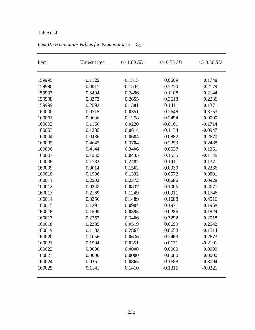
230
Table C.4 Item Discrimination Values for Examination 3 – CX4 Item Unrestricted +/- 1.00 SD +/- 0.75 SD +/- 0.50 SD 159995 -0.1125 -0.1515 0.0609 0.1748 159996 -0.0017 -0.1534 -0.3230 -0.2179 159997 0.3494 0.2456 0.1108 0.2144 159998 0.3372 0.2655 0.3618 0.2236 159999 0.2592 0.1381 0.1411 0.1371 160000 0.0715 -0.0351 -0.2648 -0.3753 160001 -0.0636 -0.1278 -0.2494 0.0000 160002 0.1160 0.0220 -0.0161 -0.1714 160003 0.1235 0.0614 -0.1134 -0.0947 160004 -0.0436 -0.0684 0.0882 0.2670 160005 0.4647 0.3704 0.2259 0.2488 160006 0.4144 0.3406 0.0537 0.1261 160007 0.1342 0.0433 0.1535 -0.1148 160008 0.1732 0.2487 0.1411 0.1371 160009 0.0014 0.1562 -0.0930 0.2236 160010 0.1508 0.1332 0.0572 0.3801 160011 0.2503 0.2372 -0.0686 0.0928 160012 -0.0345 -0.0837 0.1086 0.4677 160013 0.2169 0.1249 -0.0911 -0.1746 160014 0.3356 0.1489 0.1688 0.4516 160015 0.1391 0.0904 0.1971 0.1958 160016 0.1500 0.0395 0.0286 0.1824 160017 0.2353 0.3406 0.3292 0.2018 160018 0.2385 0.0519 0.0699 0.2542 160019 0.1183 0.2867 0.0658 -0.1514 160020 0.1056 0.0636 -0.2469 -0.2673 160021 0.1994 0.0351 0.0671 -0.2191 160022 0.0000 0.0000 0.0000 0.0000 160023 0.0000 0.0000 0.0000 0.0000 160024 -0.0251 -0.0865 -0.1688 -0.3094 160025 0.1141 0.1410 -0.1315 -0.0221

231
Table C.4 (continued) Item Discrimination Values for Examination 3 – CX4 Item Unrestricted +/- 1.00 SD +/- 0.75 SD +/- 0.50 SD 160026 0.1059 0.0673 -0.2494 0.0000 160027 0.0230 -0.1348 0.0887 0.3801 160028 0.2308 0.1164 0.2614 0.0947 160029 0.3289 0.2016 0.1515 0.1398 160030 0.2980 0.1099 0.0856 0.0522 160031 0.2154 0.2059 -0.0889 -0.3438 160032 0.4353 0.2836 0.0733 -0.0510 160033 -0.0930 -0.2132 -0.2163 -0.2297 160034 0.4090 0.2511 -0.0684 -0.0419 160035 0.2824 0.1248 -0.0384 -0.0949 160036 0.0739 0.2149 0.3432 0.2346 160037 -0.0380 -0.0740 -0.1439 -0.2542 160038 0.0829 0.1826 0.0144 -0.0153 160039 0.1151 0.0277 0.0671 0.0643 160040 -0.0036 -0.0875 0.2123 0.0153 160041 0.4053 0.2247 0.3350 0.2120 160042 0.1553 0.0190 0.2242 0.0203 160043 0.1101 0.2464 0.1201 0.1161 160044 0.1223 -0.0710 -0.0701 -0.0966 160045 0.1300 0.1661 -0.0686 0.0928 160046 0.2300 0.1515 0.1265 0.2166 160047 0.1708 0.3145 -0.1248 -0.1824 160048 0.2581 0.0806 0.1528 -0.1175 160049 0.0586 0.0298 0.2259 0.2644 160050 0.2836 0.0000 0.0000 0.0000 160051 0.3579 0.2550 0.0066 0.2909 160052 0.1241 0.0965 0.2025 0.0015 160053 0.2348 0.1863 0.3718 0.2652 160054 0.1140 0.0117 0.2894 0.1072 160055 0.2920 0.3703 0.1343 0.2475 160056 0.2966 0.0555 0.0965 0.0928

232
Table C.4 (continued) Item Discrimination Values for Examination 3 – CX4 Item Unrestricted +/- 1.00 SD +/- 0.75 SD +/- 0.50 SD 160057 0.3838 0.3438 0.4976 0.2236 160058 0.0012 0.1526 0.0887 0.0682 160059 0.2883 0.2140 0.0856 0.0522 160060 0.0000 0.0000 0.0000 0.0000 160061 0.2186 0.0521 0.1087 0.0671 160062 0.1056 0.1597 0.2102 0.2652 160063 0.0365 0.0753 0.2254 0.3032 160064 0.2481 0.0790 0.0340 -0.3226 160065 -0.0272 0.0335 0.1914 0.3305 160066 -0.1009 -0.1216 -0.0066 -0.1134 160067 0.0136 -0.0820 -0.0413 -0.1539 160068 0.0390 0.0875 0.1727 0.2236 160069 0.2224 0.0820 0.0344 0.2220 160070 0.0423 -0.0521 0.0596 0.0015 160071 0.1943 0.1923 0.0853 0.0308 160072 0.2186 0.2338 -0.0384 -0.0949 160073 0.2013 0.2429 0.2322 0.5543 160074 0.3289 0.2511 -0.0905 -0.0783 160075 0.0000 0.0000 0.0000 0.0000 160076 0.1443 -0.0174 0.1353 0.1181 160077 0.0059 0.0351 -0.1347 -0.1510 160078 0.1822 0.0318 0.0701 -0.0235 160079 0.3248 0.1978 0.3073 0.1641 160080 0.1056 -0.1002 0.1101 0.0792 160081 0.1882 0.2174 0.1201 0.1439 160082 0.1301 0.0375 0.0733 -0.2166 160083 0.1376 0.1450 0.0991 -0.2166 160084 0.2800 0.1803 -0.0930 -0.1945 160085 0.1580 0.1909 0.1857 0.1958 160086 0.1300 0.1663 0.0428 -0.1748 160087 0.1955 0.1131 0.1093 0.4669

233
Table C.4 (continued) Item Discrimination Values for Examination 3 – CX4 Item Unrestricted +/- 1.00 SD +/- 0.75 SD +/- 0.50 SD 160088 -0.0804 -0.1547 -0.3549 -0.3690 160089 0.2772 0.0912 0.0198 -0.0402 160090 -0.0300 -0.1330 -0.1315 -0.0221 160526 0.2836 0.0000 0.0000 0.0000 160527 0.2211 0.0573 0.0477 -0.1991 160528 0.1479 0.1909 0.2109 0.0098 160529 -0.0272 0.0708 -0.1234 -0.0179 160530 0.1396 0.0847 -0.1255 0.0827 160531 0.1950 0.2541 -0.0250 0.1398 160532 0.0518 0.1144 0.2254 0.3032 160533 0.2074 0.1546 0.0586 0.0354 160534 0.0000 0.0000 0.0000 0.0000 160535 0.2356 0.0222 -0.0399 0.0654 160536 0.0713 0.0388 -0.1038 -0.4054 160537 0.2885 -0.0677 0.2459 0.3078 160538 0.1169 -0.0576 -0.0173 0.0403 160539 0.0901 -0.0641 -0.2021 -0.1174 160540 0.1639 0.1748 -0.0576 -0.1174 160541 0.3539 0.1281 -0.0250 0.1398 160542 0.1824 0.1611 0.2504 0.0730 160543 0.0649 -0.1348 -0.1083 -0.2448 160544 0.1833 0.0336 0.0671 0.0643 160545 0.0954 -0.0515 -0.1966 -0.3338 160546 0.0000 0.0000 0.0000 0.0000 160547 0.2811 0.3158 0.2413 0.2642 160548 0.2629 0.1228 0.2683 0.1235 160549 0.2824 0.1144 0.2254 0.3032 160550 0.4042 0.2292 0.0767 -0.0557 160551 0.2205 0.1160 0.0025 -0.0751 160552 0.3101 0.1704 -0.2494 0.0000 160553 0.1476 0.1053 0.2494 0.0792

234
Table C.4 (continued) Item Discrimination Values for Examination 3 – CX4 Item Unrestricted +/- 1.00 SD +/- 0.75 SD +/- 0.50 SD 160554 0.2015 0.2220 0.0000 0.0000 160555 0.3749 0.0000 0.0000 0.0000 160556 0.2813 0.2868 0.4625 0.2346 160557 0.3548 0.2664 -0.0551 -0.1370 160558 0.2423 0.2467 0.0384 0.1569 160559 0.2653 0.1597 0.1556 0.1371 160560 0.2133 0.0594 0.1201 0.2236 160561 0.2015 0.0067 0.0144 -0.0153 160562 -0.0636 -0.1278 -0.2494 0.0000 160563 0.1022 0.2429 0.0991 -0.0095 160564 0.2586 0.1070 0.3309 0.0000 160565 0.1646 0.1704 0.1344 0.1503 160566 0.2540 0.0555 0.1344 0.1503 160567 0.0320 0.1434 0.3197 0.4342 160568 0.0281 -0.2086 0.0000 0.0000 160569 0.2538 0.0784 0.2145 0.2599 160570 0.2961 0.1923 0.2856 0.1371 160571 0.1201 0.1228 0.1926 0.2024 160572 0.2302 -0.0027 0.1556 0.1371 160573 0.2998 0.2811 0.3786 0.3438 160574 0.2106 0.0336 0.0671 0.0643 160575 0.0609 0.0119 0.0671 0.0643 160576 0.0652 -0.1216 -0.1151 -0.0274 160577 0.1216 0.0708 -0.0930 0.2236 160578 0.1544 0.0000 0.0000 0.0000

235
Table C.5 Item Discrimination Values for Examination 3 – CX5 Item Unrestricted +/- 1.00 SD +/- 0.75 SD +/- 0.50 SD 159995 -0.1125 0.0526 0.0388 0.0624 159996 -0.0017 0.3743 0.2466 0.7057 159997 0.3494 0.2443 0.5114 0.3119 159998 0.3372 0.2454 0.3812 0.2205 159999 0.2592 -0.1505 -0.6117 -0.1953 160000 0.0715 0.1734 0.1165 0.1871 160001 -0.0636 0.0000 0.0000 0.0000 160002 0.1160 -0.1681 0.2018 0.8090 160003 0.1235 0.4983 0.2202 0.5300 160004 -0.0436 -0.1832 -0.5157 -0.5300 160005 0.4647 0.8629 0.7721 0.5300 160006 0.4144 0.0681 0.2719 -0.2205 160007 0.1342 -0.1206 -0.1905 0.1871 160008 0.1732 -0.2353 -0.2202 -0.5300 160009 0.0014 0.0000 0.0000 0.0000 160010 0.1508 0.2096 0.7193 0.8090 160011 0.2503 -0.2308 0.0147 -0.1953 160012 -0.0345 0.3208 0.7193 0.8090 160013 0.2169 -0.0128 -0.4260 -0.3627 160014 0.3356 -0.3096 -0.3710 -0.4411 160015 0.1391 0.1206 -0.1942 -0.3119 160016 0.1500 0.1084 -0.0301 -0.2205 160017 0.2353 0.1538 0.1103 0.3529 160018 0.2385 0.2539 0.3495 -0.0882 160019 0.1183 0.2539 0.4272 0.6862 160020 0.1056 0.0984 -0.2466 -0.7057 160021 0.1994 -0.0201 -0.2908 -0.3088 160022 0.0000 0.0000 0.0000 0.0000 160023 0.0000 0.0000 0.0000 0.0000 160024 -0.0251 -0.2722 0.0000 0.0000 160025 0.1141 -0.0879 -0.2466 -0.7057

236
Table C.5 (continued) Item Discrimination Values for Examination 3 – CX5 Item Unrestricted +/- 1.00 SD +/- 0.75 SD +/- 0.50 SD 160026 0.1059 -0.1969 0.0000 0.0000 160027 0.0230 0.1796 0.0147 -0.1953 160028 0.2308 0.1502 -0.2908 -0.3088 160029 0.3289 0.0793 0.1905 0.4852 160030 0.2980 0.1889 -0.4709 -0.3529 160031 0.2154 -0.2136 0.1103 -0.3119 160032 0.4353 0.2919 0.5315 0.7057 160033 -0.0930 -0.5759 -0.4512 -0.5734 160034 0.4090 0.3746 0.1304 0.6862 160035 0.2824 -0.3331 -0.0673 0.3069 160036 0.0739 0.4877 0.3812 0.2205 160037 -0.0380 0.0000 0.0000 0.0000 160038 0.0829 -0.3475 0.0000 0.0000 160039 0.1151 0.0984 -0.2466 -0.0279 160040 -0.0036 -0.4156 -0.4260 -0.3627 160041 0.4053 0.6563 0.6919 0.3627 160042 0.1553 0.3764 0.2018 0.8090 160043 0.1101 -0.3465 -0.4550 0.0000 160044 0.1223 0.6155 0.6602 0.4411 160045 0.1300 -0.1241 -0.1028 -0.3627 160046 0.2300 -0.1206 0.1942 0.3119 160047 0.1708 -0.2030 -0.3510 -0.0624 160048 0.2581 0.2408 0.1103 -0.3119 160049 0.0586 -0.1969 0.0000 0.0000 160050 0.2836 0.2096 -0.0673 -0.4411 160051 0.3579 -0.2931 -0.3812 -0.2205 160052 0.1241 -0.2784 -0.1028 -0.3627 160053 0.2348 -0.1940 -0.6117 -0.1953 160054 0.1140 0.2855 0.1165 0.1871 160055 0.2920 0.0681 0.2719 -0.2205 160056 0.2966 0.1973 0.5606 0.4852

237
Table C.5 (continued) Item Discrimination Values for Examination 3 – CX5 Item Unrestricted +/- 1.00 SD +/- 0.75 SD +/- 0.50 SD 160057 0.3838 0.3277 -0.1165 -0.1871 160058 0.0012 0.0000 0.0000 0.0000 160059 0.2883 0.2842 0.8296 0.8822 160060 0.0000 0.0000 0.0000 0.0000 160061 0.2186 0.1978 -0.2106 -0.1764 160062 0.1056 0.4054 0.3670 0.3069 160063 0.0365 -0.1969 0.0000 0.0000 160064 0.2481 -0.0681 -0.3495 -0.5614 160065 -0.0272 -0.2722 0.0000 0.0000 160066 -0.1009 -0.5016 -0.5916 -0.4366 160067 0.0136 0.1502 0.2018 -0.0441 160068 0.0390 0.0000 0.0000 0.0000 160069 0.2224 0.4092 0.3495 0.5614 160070 0.0423 -0.1797 -0.2202 -0.5300 160071 0.1943 0.0549 0.0224 -0.3088 160072 0.2186 -0.0635 0.7193 0.8090 160073 0.2013 -0.2855 -0.1165 -0.1871 160074 0.3289 0.2030 0.0388 0.0624 160075 0.0000 0.0000 0.0000 0.0000 160076 0.1443 0.3208 0.1121 -0.1764 160077 0.0059 0.2842 0.3510 0.0624 160078 0.1822 0.1502 0.2018 0.8090 160079 0.3248 -0.0929 0.0388 0.0624 160080 0.1056 0.3764 0.2018 0.8090 160081 0.1882 -0.0403 0.3670 0.3069 160082 0.1301 -0.2094 0.0224 -0.3088 160083 0.1376 -0.2919 0.0224 -0.3088 160084 0.2800 0.4505 -0.0301 -0.2205 160085 0.1580 -0.1241 0.0147 -0.1953 160086 0.1300 -0.4149 -0.5826 -0.3088 160087 0.1955 0.6155 0.6602 0.4411

238
Table C.5 (continued) Item Discrimination Values for Examination 3 – CX5 Item Unrestricted +/- 1.00 SD +/- 0.75 SD +/- 0.50 SD 160088 -0.0804 0.0000 0.0000 0.0000 160089 0.2772 -0.1734 -0.1942 0.3529 160090 -0.0300 -0.1241 -0.1028 -0.3627 160526 0.2836 0.2096 -0.0673 0.3069 160527 0.2211 0.0879 0.2466 0.0279 160528 0.1479 0.0290 -0.2202 -0.5300 160529 -0.0272 0.0000 0.0000 0.0000 160530 0.1396 -0.3498 -0.3710 -0.4411 160531 0.1950 -0.1681 0.2018 0.8090 160532 0.0518 0.0000 0.0000 0.0000 160533 0.2074 -0.0684 -0.1028 -0.3627 160534 0.0000 0.0000 0.0000 0.0000 160535 0.2356 0.0000 0.0000 0.0000 160536 0.0713 -0.6218 -0.6951 0.0000 160537 0.2885 0.0279 0.1165 0.8822 160538 0.1169 0.0549 -0.0673 -0.4411 160539 0.0901 0.1331 0.0388 0.0624 160540 0.1639 -0.0929 -0.4312 -0.8822 160541 0.3539 0.6161 0.1570 0.5734 160542 0.1824 0.2842 0.2707 0.6175 160543 0.0649 -0.2308 -0.5157 -0.5300 160544 0.1833 0.4054 0.3670 0.3069 160545 0.0954 -0.4021 0.0000 0.0000 160546 0.0000 0.0000 0.0000 0.0000 160547 0.2811 -0.1070 0.1121 -0.1764 160548 0.2629 0.3475 0.0000 0.0000 160549 0.2824 -0.0879 0.3670 0.3069 160550 0.4042 0.3498 0.3710 0.4411 160551 0.2205 -0.3244 -0.7721 -0.5300 160552 0.3101 0.2931 -0.0501 -0.5614 160553 0.1476 0.5016 0.6719 0.5614

239
Table C.5 (continued) Item Discrimination Values for Examination 3 – CX5 Item Unrestricted +/- 1.00 SD +/- 0.75 SD +/- 0.50 SD 160554 0.2015 0.0290 -0.2202 -0.5300 160555 0.3749 0.7657 0.8296 0.8822 160556 0.2813 0.1538 0.0301 0.2205 160557 0.3548 0.3680 0.7521 0.6862 160558 0.2423 -0.1832 0.1321 -0.0279 160559 0.2653 0.3407 0.4709 0.3529 160560 0.2133 0.3208 0.1121 -0.1764 160561 0.2015 0.6313 0.7193 0.8090 160562 -0.0636 0.0000 0.0000 0.0000 160563 0.1022 -0.0032 0.1103 -0.3119 160564 0.2586 0.2842 0.2707 -0.0624 160565 0.1646 0.1043 -0.1028 -0.3627 160566 0.2540 0.2931 0.3812 0.2205 160567 0.0320 0.0290 -0.2202 -0.5300 160568 0.0281 -0.1969 0.0000 0.0000 160569 0.2538 0.3407 0.0301 0.2205 160570 0.2961 0.2030 0.4312 0.1871 160571 0.1201 -0.1026 -0.1121 0.1764 160572 0.2302 0.1104 0.4709 0.3529 160573 0.2998 0.2094 -0.2018 -0.8090 160574 0.2106 0.6313 0.7193 0.8090 160575 0.0609 -0.0684 -0.5157 -0.5300 160576 0.0652 0.0201 0.2908 0.3088 160577 0.1216 -0.1084 0.1905 0.4852 160578 0.1544 -0.1216 -0.4550 0.0000

240
REFERENCES
Alsawalmeh, Y., & Feldt, L. (1994). A modification of Feldt's test of the equality of two dependent alpha coefficients. Psychometrika, 59(1), 49-57.
American Educational Research Association, American Psychological Association, National
Council on Measurement in Education. (1999). Standards for educational and psychological testing. Washington, DC: American Psychological Association.
American National Standards Institute. (2013). ANSI Overview. Retrieved from
http://www.ansi.org/about_ansi/overview/overview.aspx?menuid=1. Atkinson, D. (2012). Legal issues and considerations for standard setting. In G. J. Cizek
(Ed.), Setting performance standards: Foundations, methods, and innovations (2nd ed.) (pp. 485-501). New York: Routledge.
Barnhart, H.X., & Williamson J.M. (2002). Weighted least-squares approach for comparing
correlated kappa, Biometrics, 58, 1012–1019. Beuchert, A. K., & Mendoza, J. L. (1979). A Monte Carlo comparison of ten discrimination
indices. Journal of Educational Measurement, 16(2), 109-117. Brennan, R. L. (1972). A generalized upper-lower item discrimination index. Educational
and Psychological Measurement, 32, 289-303. Buckendahl, C. W., & Davis-Becker, S. L. (2012). Setting passing standards for
credentialing programs. In G. J. Cizek (Ed.), Setting performance standards: Foundations, methods, and innovations (2nd ed.) (pp. 485-501). New York: Routledge.
Burton, R. (2001). Do item-discrimination indices really help us to improve our
tests? Assessment and Evaluation in Higher Education, 26(3), 213-20. Cizek, G. J. (2012a). An introduction to contemporary standard setting. In G. J. Cizek
(Ed.), Setting performance standards: Foundations, methods, and innovations (2nd ed.) (pp. 3-14). New York: Routledge.
Cizek, G. J. (2012b). Defining and distinguishing validity: Interpretations of score meaning
and justification of test use. Psychological Methods, 17(1), 31-43. Clauser, B. E., Margolis, M. J., & Case, S. M. (2006). Testing for licensure and certification
in the professions. In R. L. Brennan (Ed.). Educational measurement (4th ed.) (pp. 701-732). Westport, CT: Praeger.
Cohen, Jacob (1960). A coefficient of agreement for nominal scales. Educational and
Psychological Measurement 20(1), 37–46.
241
Crocker, L., & Algina, J. (2008). Introduction to classical and modern test theory.
Mason, OH: Cengage Learning. Cronbach, L. J. (1951). Coefficient alpha and the internal structure of tests. Psychometrika, 16, 297-334. Diedenhofen, B. (2013). cocron: Statistical comparisons of two or more alpha coefficients
(Version 0.01-5). Retrieved from http://r.birkdiedenhofen.de/pckg/cocron/. Donner, A., Shoukri, M., Klar, N., & Bartfay E. (2000). Testing the equality of two
dependent kappa statistics. Statistics in Medicine, 19, 373-387. Downing, S. M. (2006). Twelve steps for effective test development. In S. M. Downing &
T. M. Haladyna (Eds.), Handbook of test development (pp. 3-25). Mahwah, NJ: Erlbaum.
DuBois, P. H. (1970). A history of psychological testing. Boston: Allyn and Bacon. Ebel, R. L. (1965). Measuring educational achievement. Englewood Cliffs, NJ: Prentice
Hall. Ebel, R. L. (1967). The relation of item discrimination to test reliability. Journal of
Educational Measurement, 4(3), 125-128. Fan, X. (1998). Item response theory and classical test theory: An empirical comparison of
their item/person statistics. Educational and Psychological Measurement, 58(3), 357-381.
Farish, S. J. (1984). Investigating item stability: An empirical investigation into the
variability of item statistics under conditions of varying sample design and sample size. Occasional Paper No. 18. Hawthorn, Australia: Australian Council of Educational Research.
Fletcher, T. D. (2010). Psychometric: Applied psychometric theory. Retrieved from http://CRAN.R-project.org/package=psychometric. Fleiss, J. L. (1981). Statistical methods for rates and proportions (2nd ed.), New York:
Wiley.
Fox, J., & Weisberg, S. (2011). An {R} companion to applied regression (2nd ed.). Thousand Oaks CA: Sage.
García Ballester, L., McVaugh, M. R., & Rubio-Vela, A. (1989). Medical licensing and
learning in fourteenth-century Valencia. Philadelphia: American Philosophical Society.

242
Greenhouse, S. W., & Geisser, S. (1959). On methods in the analysis of profile data. Psychometrika, 24, 95-112.
Haertel, E. H. (2006). Reliability. In R. L. Brennan (Ed.). Educational measurement, 4th ed. (pp. 65-110). Westport, CT: Praeger. Hambleton, R. K., & Jones, R. W. (1993). Comparison of classical test theory and item
response theory and their applications to test development. Educational Measurement: Issues and Practice, 12(3), 38-47.
Hambleton, R. K., & Novick, M. R. (1973). Toward an integration of theory and method for
criterion-referenced tests. Journal of Educational Measurement, 10, 159-170. Harris, D. J., & Subkoviak, M. J. (1986). Item analysis: A short-cut statistic for mastery tests.
Educational and Psychological Measurement, 46, 495-507. Huck, S. W. (2008). Reading statistics and research (5th ed.). Boston, MA: Pearson. Hunyh, H. (1976). On the reliability of decisions in domain-referenced testing. Journal of
Educational Measurement, 13, 253-264. International Organization for Standardization. (2013). About ISO. Retrieved from
http://www.iso.org/iso/home/about.htm. Jones, P., Smith, R. W., & Talley, D. (2006). Developing test forms for small-scale
achievement testing systems. In S. M. Downing & T. M. Haladyna (Eds.), Handbook of test development (pp. 487-526). Mahwah, NJ: Erlbaum.
Kane, M. T. (1992). An argument-based approach to validity. Psychological Bulletin, 112(3),
527-535. Kelley, T. L. (1939). The selection of upper and lower groups for the validation of test
items. Journal of Educational Psychology, 30(1), 17-24. Lipsitz, S. R., Williamson, J., Klar, N., Ibrahim, J., & Parzen, M. (2001). A simple method
for estimating a regression model for κ between a pair of raters. Journal of the Royal Statistical Society, 164(3), 449-465.
Livingston, S. A. (2006). Item Analysis. In S. M. Downing & T. M. Haladyna (Eds.),
Handbook of test development (pp. 421-441). Mahwah, NJ: Erlbaum. Lord, F. M., & Novick, M. R. (1968). Statistical theories of mental test scores. Reading, MA:
Addison-Wesley.

243
Luecht, R. M. (2006). Designing tests for pass-fail decisions using item response theory. In S. M. Downing & T. M. Haladyna (Eds.), Handbook of test development (pp. 575-598). Mahwah, NJ: Erlbaum.
Mauchly, J. W. (1940). Significance test for sphericity of a normal n-variate distribution. The
Annals of Mathematical Statistics, 11(2), 204-209. McKenzie, D. P., Mackinnon, A. J., Peladeau, N., Onghena, P., Bruce, P., Clark, D., . . .
McGorry, P. D. (1996). Comparing correlated kappas by resampling: Is one level of agreement significantly different than another? Journal of Psychiatric Research, 30(6), 483-492.
Meyer, J. P. (2013). jMetrik. Retrieved from http://www.itemanalysis.com/index.php. Millman, J., & Greene, J. (1989). The specification and development of tests of achievement
and ability. In R. L. Linn (Ed.), Educational Measurement (3rd ed.). Washington, DC: American Council on Education.
No Child Left Behind (NCLB) Act. (2002). P.L. 107-110.(20 U.S.C. 6301-6578). Odueyungbo, A., Thabane, L., & Marlke-Reid, M. (2009). Tips on overlapping confidence
intervals and univariate linear models: Adefowope Odueyungbo, Lehana Thabane and Maureen Markle-Reid discuss ways to improve estimates from various linear regression models and derive findings when confidence intervals overlap. Nurse Researcher, 16(4), 73.
Oosterhof, A. C. (1976). Similarity of various item discrimination indices. Journal of
Educational Measurement, 13(2), 145-150. Pearson, K. (1909). On a new method of determining a correlation between a measured
character of A and a character of B, of which only the percentage of cases wherein B exceeds (or falls short of) intensity is recorded for each grade of A. Biometrika, 7, 96-105.
R Core Team. (2012). R: A language and environment for statistical computing. Vienna,
Austria: R Foundation for Statistical Computing. Retrieved from http://www.R-project.org/.
Raymond, M., & Neustel, S. (2006). Determining the content of credentialing examinations.
In S. M. Downing & T. M. Haladyna (Eds.), Handbook of test development (pp. 181-224). Mahwah, NJ: Erlbaum.
Reise, S. P., & Yu, J. (1990). Parameter recovery in the graded response model using
MULTILOG. Journal of Educational Measurement, 27(2), 133-144.

244
Revelle, W. (2013) psych: procedures for personality and psychological research. Northwestern University, Evanston, IL. Retrieved from http://CRAN.R-project.org/package=psych Version = 1.3.2.
Schmeiser, C. B., & Welch, C. J. (2006). Test development. In R. L. Brennan (Ed.).
Educational measurement (4th ed.) (pp. 307-354). Westport, CT: Praeger. Subkoviak, M. J. (1976). Estimating reliability from a single administration of a criterion-
referenced test. Journal of Educational Measurement, 13, 265-275. Subkoviak, M. J. (1978). Empirical investigation of procedures for estimating reliability for
mastery tests. Journal of Educational Measurement, 15, 111-116. Swaminathan, H., Hambleton, R. K., & Algina, J. (1974). Reliability of criterion referenced
tests: A decision theoretic formulation. Journal of Educational Measurement, 11, 263-268.
Thorndike, R. L. (1982). Applied psychometrics. Boston: Houghton Mifflin. Williamson, J. M., Lipsitz, S. R., & Manatunga, A. K. (2000). Modeling kappa for measuring
dependent categorical agreement data. Biostatistics, 1(2), 191-202. Yen, W. M., & Fitzpatrick, A. R. (2006). Item response theory. In R. L. Brennan (Ed.).
Educational measurement (4th ed.) (pp. 111-153). Westport, CT: Praeger.